| Issue |
A&A
Volume 689, September 2024
|
|
|---|---|---|
| Article Number | A227 | |
| Number of page(s) | 22 | |
| Section | Cosmology (including clusters of galaxies) | |
| DOI | https://doi.org/10.1051/0004-6361/202347987 | |
| Published online | 19 September 2024 | |
A road map to cosmological parameter analysis with third-order shear statistics
III. Efficient estimation of third-order shear correlation functions and an application to the KiDS-1000 data
1
University of Bonn, Argelander-Institut für Astronomie, Auf dem Hügel 71, 53121 Bonn, Germany
2
Department of Astronomy and Astrophysics, University of California, Santa Cruz, 1156 High Street, Santa Cruz, CA 95064, USA
3
Universität Innsbruck, Institut für Astro- und Teilchenphysik, Technikerstr. 25/8, 6020 Innsbruck, Austria
Received:
15
September
2023
Accepted:
27
February
2024
Abstract
Context. Third-order lensing statistics contain a wealth of cosmological information that is not captured by second-order statistics. However, the computational effort it takes to estimate such statistics in forthcoming stage IV surveys is prohibitively expensive.
Aims. We derive and validate an efficient estimation procedure for the three-point correlation function (3PCF) of polar fields such as weak lensing shear. We then use our approach to measure the shear 3PCF and the third-order aperture mass statistics on the KiDS-1000 survey.
Methods We constructed an efficient estimator for third-order shear statistics that builds on the multipole decomposition of the 3PCF. We then validated our estimator on mock ellipticity catalogs obtained from N-body simulations. Finally, we applied our estimator to the KiDS-1000 data and presented a measurement of the third-order aperture statistics in a tomographic setup.
Results. Our estimator provides a speedup of a factor of ∼100–1000 compared to the state-of-the-art estimation procedures. It is also able to provide accurate measurements for squeezed and folded triangle configurations without additional computational effort. We report a significant detection of tomographic third-order aperture mass statistics in the KiDS-1000 data (S/N = 6.69).
Conclusions. Our estimator will make it computationally feasible to measure third-order shear statistics in forthcoming stage IV surveys. Furthermore, it can be used to construct empirical covariance matrices for such statistics.
Key words: gravitation / gravitational lensing: weak / methods: numerical / large-scale structure of Universe
Corresponding author; This email address is being protected from spambots. You need JavaScript enabled to view it.
© The Authors 2024
 Open Access article, published by EDP Sciences, under the terms of the Creative Commons Attribution License (https://creativecommons.org/licenses/by/4.0), which permits unrestricted use, distribution, and reproduction in any medium, provided the original work is properly cited.
This article is published in open access under the Subscribe to Open model. This email address is being protected from spambots. You need JavaScript enabled to view it. to support open access publication.
1. Introduction
The most widely used set of statistics for extracting cosmological information from galaxy or weak gravitational lensing surveys is related to N-point correlation functions (NPCF s). Estimating those quantities from the position or shape of a set of observed tracers, one reveals parts of the statistical properties of the underlying large-scale cosmic structure. In particular, for weak gravitational lensing surveys, the analysis of shear two-point correlation functions (2PCFs) and their harmonic analog, the power spectrum, have made it possible to put tight constraints on the matter clustering parameter,  , where σ8 is the normalization of the matter power spectrum and Ωm is the matter density parameter (Heymans et al. 2013; Hildebrandt et al. 2017; Troxel et al. 2018; Hikage et al. 2019; Hamana et al. 2020; Asgari et al. 2021; Amon et al. 2022; Secco et al. 2022; Dalal et al. 2023; Li et al. 2023).
While most of the theoretical and observational work has been done at the second-order level, it is well known that through this choice one is sensitive only to the Gaussian information of the density field. To extract additional information including contributions from nonlinear structure formation, one needs to resort to other higher-order statistics, some of which are related to higher-order moments (Jain & Seljak 1997; Schneider et al. 1998; Vicinanza et al. 2018; Gatti et al. 2020), peaks (Kruse & Schneider 1999; Hamana et al. 2004; Harnois-Déraps et al. 2021), the one-point probability distribution function (Patton et al. 2017; Barthelemy et al. 2020; Boyle et al. 2021; Giblin et al. 2023), or the topological properties (Kratochvil et al. 2012; Parroni et al. 2020; Heydenreich et al. 2022) of the density field. Besides the gain in cosmological information, it has been shown that when performing a joint analysis together with second-order statistics, higher-order statistics can also break degeneracies between parameters of cosmological, astrophysical, or systematic origin, and therefore have the potential to yield much tighter cosmological constraints (Kilbinger & Schneider 2005; Takada & Jain 2003; Semboloni et al. 2008; Pyne & Joachimi 2021).
Higher-order statistics from the correlation function hierarchy consist of the (N > 2)-point correlation functions, of which the three-point correlation function (3PCF) is the most prominent example (Schneider & Lombardi 2003; Zaldarriaga & Scoccimarro 2003). Besides the challenges in accurately modeling cosmological and observational effects on the shape of the 3PCF (Takada & Jain 2003; Heydenreich et al. 2023), it is also computationally much more expensive to estimate them, compared to those of the 2PCF. A naive estimator would require all triplets of tracers to be put into a predefined set of bins describing the triplets’ configuration. The resulting computational complexity of a survey of Ngal tracers is 𝒪(Ngal3), rendering this brute-force approach computationally prohibitive. To facilitate an estimation of the 3PCF of scalar (spin-0) and polar (spin-2) observables for current surveys, kd-tree based methods have been developed (Jarvis et al. 2004; Zhang & Pen 2005; Kilbinger et al. 2014) and applied to a wide range of datasets (Bernardeau et al. 2002; Semboloni et al. 2011; Fu et al. 2014; Secco et al. 2022). Even though the computational speedup compared to the brute-force estimator is remarkable, it is most likely still too time-consuming to apply it to stage IV cosmic shear surveys like Euclid (Laureijs et al. 2011) or the Vera Rubin Observatory Legacy Survey of Space and Time (Ivezić et al. 2019). A different class of estimators has been tailored toward the multipole components of the NPCF s of scalar fields (Chen & Szapudi 2005; Slepian & Eisenstein 2015; Philcox et al. 2022). As the multipoles can be estimated in quadratic time complexity for a discrete galaxy catalog, or with an Npixlog(Npix) scaling for data distributed on a grid of Npix pixels, this estimation strategy makes it feasible to efficiently and accurately measure higher-order correlation functions in large datasets. For example, the first measurement of the 4PCF of the scalar galaxy position field was presented in Hou et al. (2023) and Philcox (2022).
In this work, we extend the multipole decomposition of the scalar 3PCF to the natural components of the 3PCF associated with spin-2 tracer fields, such as weak lensing shear. Additionally, we construct an efficient estimator that adaptively switches between a discrete and grid-based prescription for triangle sides of different lengths. With those modifications, we can measure the full 3PCF of any triangle configuration in a stage-III survey in a few central processing unit (CPU) hours without significantly sacrificing accuracy compared to the brute-force estimator.
This work belongs to a series of papers that aim to undertake a cosmological parameter analysis using third-order shear statistics. Heydenreich et al. (2023) introduces an analytical model for the third-order aperture statistics based on the Bihalofit formula (Takahashi et al. 2020) for the matter bispectrum. In Linke et al. (2023), an analytical covariance matrix for the third-order aperture statistics is derived in the presence of a finite survey extent. Burger et al. (2024) extends the analytical model to a tomographic setting, includes methods to account for the impact of intrinsic alignments and baryonic feedback, and presents a cosmological analysis using a joint data vector of the COSEBIs and the third-order aperture mass statistics measured in the KiDS-1000 data.
This paper is structured as follows. In Sect. 2, we introduce the shear 3PCF and their natural components, Γμ. In Sect. 3, we derive our estimator of the Γμ and discuss some approximations. In Sect. 4, we validate our estimator on a large suite of N-body simulations, the SLICS ensemble, and compare it with measurements obtained with TREECORR (Jarvis et al. 2004). In Sect. 5, we introduce the third-order aperture measures, show how they can be obtained from our shear 3PCF estimator, and validate our implementation. In Sect. 6, we apply our estimator to the fourth data release of the Kilo Degree Survey (Kuijken et al. 2019, hereafter KiDS-1000). After obtaining an empirical estimate of the expected correlation matrix for the KiDS-1000 data from a large suite of mock catalogs we present our measurement of the third-order aperture statistics in the KiDS-1000 data. We conclude in Sect. 7.
2. Third-order measures of cosmic shear
This section aims to introduce the main concepts related to weak gravitational lensing with an emphasis on the third-order shear correlation functions (for extensive reviews of the weak gravitational lensing, see Bartelmann & Schneider 2001; Kilbinger 2015; Dodelson 2017; Mandelbaum 2018). In order to keep the notation concise, we do not consider tomographic setups in this and the following section but collect the corresponding expressions in Sect. 3.5. Furthermore, we do not consider higher-order effects like reduced shear, source redshift clustering, or astrophysical effects, such as intrinsic alignments.
2.1. Basic notions
The two fundamental quantities in weak gravitational lensing are the convergence, κ, and the shear, γ, which describe the isotropic stretching and distortion experienced by a light bundle propagating through spacetime. The convergence, κ, can be written as a weighted projection of the density contrast, δ, along the line of sight:
![Mathematical equation: $$ \begin{aligned} \kappa (\boldsymbol{\theta }) = \int _0^{\chi _{\mathrm{max} }} \mathrm{d} \chi \prime W(\chi \prime ) \ \delta \left[f_K(\chi \prime )\boldsymbol{\theta };\chi \prime \right] \ , \end{aligned} $$](/articles/aa/full_html/2024/09/aa47987-23/aa47987-23-eq2.gif) (1)
(1)
where the associated projection kernel, W, is defined as
![Mathematical equation: $$ \begin{aligned} W(\chi ) \equiv \frac{3{\Omega _{\mathrm{m} }} H_0^2}{2c^2} \frac{f_K(\chi )}{a(\chi )} \int _{z(\chi )}^{\infty } \mathrm{d} z\prime n(z\prime ) \frac{f_K[\chi (z^{\prime })-\chi ]}{f_K[\chi (z\prime )]} ,\end{aligned} $$](/articles/aa/full_html/2024/09/aa47987-23/aa47987-23-eq3.gif) (2)
(2)
and fK[χ(z)] denotes the comoving angular diameter distance of the comoving radial distance, χ, at redshift, z. We introduced the dimensionless matter density parameter, Ωm, and the Hubble constant, H0, as well as the scale factor, a, and the source redshift distribution, n(z). For the remainder of this work, we assume a flat universe for which fK(χ)=χ.
The components of the complex shear field, γ, can be characterized with respect to a Cartesian coordinate frame, γc ≡ γ1 + iγ2. To evaluate the shear at position θ in a reference frame, which is rotated by an angle, ζ, with respect to the Cartesian basis, one has
![Mathematical equation: $$ \begin{aligned} \gamma (\boldsymbol{\theta };\zeta ) \equiv -\left[{\gamma _{\mathrm{t} }}(\boldsymbol{\theta };\zeta ) + {\mathrm{i} } \gamma _\times (\boldsymbol{\theta };\zeta )\right] \equiv -\gamma _{\mathrm{c} }(\boldsymbol{\theta }) \ \mathrm{e} ^{-2{\mathrm{i} }\zeta } \ , \end{aligned} $$](/articles/aa/full_html/2024/09/aa47987-23/aa47987-23-eq4.gif) (3)
(3)
where we introduced the tangential (γt) and cross-components (γ×) of the shear with respect to the projection direction, ζ.
2.2. The shear three-point correlation function and its natural components
Due to the polar nature of the shear, there are eight different real-valued components for its three-point correlator. Schneider & Lombardi (2003) regroup those components into four complex-valued natural components, Γμ, that do not mix and only transform by a particular phase factor under rotations of the corresponding triangle. Parameterizing a triangle as depicted in Fig. 1 and choosing some arbitrary projection, [BOLD]𝒫, in which the individual shear components are rotated by angles, ζi, we defined the natural components of the shear 3PCF as1
 (4)
(4)
 (5)
(5)
 (6)
(6)
 (7)
(7)
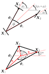 |
Fig. 1. Upper panel: Parameterization of a triplet of shears used in this work. For some shears at position X1, we denote the connecting lines to the two other shears as ϑi and the enclosing angle as ϕ. The dashed red lines show the directions of the × projection Eq. (9) for which the three projection axes intersect in X1. Lower panel: Definition of the geometric quantities involved in the centroid projection Eq. (10). We see that the q vectors connect the centroid of the triangle with the triangles’ vertices. |
where ϑi ≡ |ϑi| and we assumed that the projection directions, ζi, are defined in terms of the vertices of the triangle; this implies that the natural components are invariant under rotations of the triangle such that a parameterization in terms of three variables is sufficient. We note that any of the natural components can be written in terms of the elements
 (8)
(8)
where we introduced shorthand notation like γttt ≡ ⟨γtγtγt⟩ for the various triple products of shears (Schneider & Lombardi 2003). Inverting the relations (4)–(7), one can relate the components in Eq. (8) to the natural components.
2.3. Choice of projections for the shear three-point correlation function
In this work, we employed two particular projections. The first of them, which we dubbed the × projection, is defined by the rotation angles
 (9)
(9)
and the corresponding projection axes are depicted in the upper panel of Fig. 1. As we will see later, this projection turns out to be useful for the estimator derived in Sect. 3. For the second projection shown in the lower panel of Fig. 1, we first defined the centroid of the triangle as the intersection of its three medians and then projected the shear at position Xi along the direction, qi, of the median passing through Xi:
 (10)
(10)
where the qi are given as
 (11)
(11)
and where we defined  . The corresponding
  are useful for connecting the shear 3PCF to the third-order aperture statistics and are being used by other estimators for the 3PCF such as TREECORR.
We can convert between the two projections using Eq. (3). For example, the zeroth natural component in the × projection can be written as
from which one can immediately read off Γ0cent. Repeating similar computations for the other components and using φ2 = φ1 + ϕ, we arrived at
 (12)
(12)
 (13)
(13)
 (14)
(14)
 (15)
(15)
where the rotation angles can be expressed as
2.4. Bin-averaged shear three-point correlation function
When estimating the Γμ𝒫 from a finite set of galaxy ellipticities, one does not have direct access to every possible triangle shape but instead collects the point triplets into radial and angular bins. Such a measurement then provides an estimator of the bin-averaged shear 3PCF,  :
:
 (16)
(16)
where for each radial bin, Θi, we have ϑi ∈ [Θlow, i, Θup, i], and where we defined Ai ≡ (Θup, i2 − Θlow, i2)/2. Similarly, for the angular bins we have ϕ ∈ [Φlow, k, Φup, k] and |ΔΦk|≡Φup, k − Φlow, k.
3. An efficient estimator of the shear three-point correlation function
Given a weak lensing catalog consisting of Ngal galaxies at positions, θi, with ellipticities2, γc, i, and weights, wi, the standard estimator of the bin-averaged natural components of the shear 3PCF consists of assigning all galaxy triplets to their corresponding triangle configuration bin and then averaging over those. In particular, the estimator of the zeroth natural component using the × projection Eq. (9) becomes
 (17)
(17)
where
 (18)
(18)
 (19)
(19)
In the preceding equations, we defined θij ≡ |θij|≡|θj − θi| and ϕijk ≡ φik − φij, with φij denoting the polar angle of θij. We furthermore introduced the bin selection function, ℬ(x ∈ X), which is at unity if x ∈ X and zero otherwise; the different combinations of the bin selection functions then specify the various triangle configurations.
3.1. Multipole decomposition
Let us first consider the numerator in Eq. (17). Instead of a discrete angular binning, one can instead perform a multipole decomposition of Υ0×. For an infinitely dense angular binning, one can decompose
 (20)
(20)
in which the nth multipole can be successively manipulated to yield
 (21)
(21)
where in the second step we inserted Eq. (18) and in the final step defined the quantity
 (22)
(22)
Repeating similar calculations for the numerators of the other three natural components, we find
 (23)
(23)
 (24)
(24)
 (25)
(25)
where for the final two equations we used
For the remainder of this work, we only write down the μ = 0 component of any equation derived from the Υμ; the expressions for the other components can be inferred from Eqs. (23)–(25).
Now switching to the denominator, Eq. (19), we can perform a derivation similar to the one leading to Eq. (21) to find the multipole expansion,
 (26)
(26)
with multipole components
 (27)
(27)
 (28)
(28)
The decomposition of the denominator has already been explored in the context of galaxy clustering in which the corresponding 3PCF is a scalar (Slepian & Eisenstein 2015; Philcox et al. 2022). Here we have shown that using the × projection, Eq. (9), gives structurally equivalent expressions for the multipole components of the 3PCF of polar fields.
Regarding the computational complexity, we see that each multipole in the decompositions of the Υμ× and 𝒩 involves a double sum over the whole ellipticity catalog, making the estimation process of the shear 3PCF formally scale as 𝒪(Ngal2). In practice, the largest separation, θmax, for which we want to compute the 3PCF might be much smaller than the survey extent; in this case, one can employ an efficient search routine that readily finds the various galaxies located in the rings around the θi. Assuming a constant runtime3 for this search algorithm, the scaling is brought down to  .
.
3.2. Grid-based approximation
While the time complexity of the multipole estimator derived in Sect. 3.1 provides a significant speedup compared to the naive estimator and is competitive with tree-based implementations, the quadratic scaling is still prohibitive for applications in stage-IV surveys. However, we note that most of the complexity stems from the largest separations for which neighboring galaxies make similar contributions to the Gndisc and Wndisc 4. If one approximates the discrete ellipticity catalog by distributing the wi and the wiγc, i on a regular spatial grid with pixel size Δ and elements wi(Δ) and (wγc)i(Δ) then for any radial bin with lower bound Θlow ≫ Δ this approximation will give very similar results to the discrete catalog. The corresponding expression for the Gn and Wn can now be reformulated in terms of a convolution:
![Mathematical equation: $$ \begin{aligned} G_n^\Delta \left({\boldsymbol{\theta }}_i^{(\Delta )};\Theta \right)&= \sum _{k=1}^{N_{\rm pix}^{\Delta }} ({ w}\gamma _{\mathrm{c} })_k^{(\Delta )} \ \mathrm{e} ^{{\mathrm{i} } n \varphi _{ik}^{(\Delta )}} \ \mathcal{B} \left(\theta _{ik}^{(\Delta )}\in \Theta \right) \nonumber \\&= \left[({ w}\gamma _{\mathrm{c} })^{(\Delta )} \star g_{n;\Theta }^{(\Delta )}\right]\left({\boldsymbol{\theta }}_i^{(\Delta )}\right) \ , \end{aligned} $$](/articles/aa/full_html/2024/09/aa47987-23/aa47987-23-eq37.gif) (29)
(29)
![Mathematical equation: $$ \begin{aligned} W_n^\Delta \left({\boldsymbol{\theta }}_i^{(\Delta )};\Theta \right)&= \left[{ w}^{(\Delta )} \star g_{n;\Theta }^{(\Delta )}\right]\left({\boldsymbol{\theta }}_i^{\left(\Delta \right)}\right) \ , \end{aligned} $$](/articles/aa/full_html/2024/09/aa47987-23/aa47987-23-eq38.gif) (30)
(30)
where all quantities with the superscript (Δ) are evaluated at the pixel centers and where “⋆” denotes the convolution operator. The transformation to multipole components, Υμ, n×, is equivalent to the discrete case (21), but the outer sum now runs over the number of pixels,  , instead of the number of galaxies:
 (31)
(31)
The possibility of using fast Fourier transform (FFT) methods for computing the convolution gives a time complexity of the grid-based estimator of  , significantly outperforming all of the previously mentioned estimators whenever applicable.
3.3. Combined estimator
For an ellipticity catalogue from a cosmic shear survey, we can now devise an efficient estimation procedure of the shear 3PCF, as is depicted in Fig. 2. In the first step, we chose a scale, θdisc, up to which the multipoles were computed using the discrete prescription outlined in Sect. 3.1. We then picked a base resolution scale, Δ1 ≡ Δ, and some coarser resolutions, Δd ≡ 2dΔ (d = 2, 3, …), and distributed the ellipticity catalog on the corresponding grids. For each of the scales, θ > θdisc, we now selected a resolution, Δi(θ), and computed the Gn using the grid-based method from Sect. 3.2. To allocate the multipoles of two scales for which the Gn were computed with different methods, the Gn with higher resolutions needed to be mapped to the coarser grid before the Υμ, n× could be updated. In particular, for the case where one of the Gn was computed via the discrete method and the other one via the grid-based one, we first defined the quantity,  , as the value of GnΔ at the pixel, p, in which the ith galaxy resides, normalized by the number of galaxies in the pth pixel. We now have
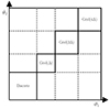 |
Fig. 2. General strategy for computing the three-point correlators used in this work. For small angular scales, we used the prescription for discrete data to compute the Gn and the Υi, n×, while for larger scales, we used the grid-based approximation with varying resolution scales, Δ. For the off-diagonal elements, we first computed the Gn of each radial bin using the corresponding method and then mapped them to the grid of the larger resolution scale from which the Υi, n× were obtained. |
 (32)
(32)
where the second sum in the second line runs over all  galaxies residing in the pth pixel. This implies that the products,
  , need to be evaluated at the true galaxy positions before they are mapped to the corresponding pixel. In Appendix A, we give more explicit details on the time and space complexity of the combined estimator.
3.4. Edge corrections
Looking back at the general form of the estimator for the shear 3PCF (Eq. 17), we see that for a brute-force-like estimator the shear 3PCF, Γμ, can be evaluated by a simple division of the two correlators, Υμ and 𝒩, for each angular and polar bin combination. On the other hand, when working on a multipole basis, we have
 (33)
(33)
To work out the analog of the division on a multipole basis, we first multiplied Eq. (17) by 𝒩 and then inserted the multipole expansion of all quantities:
 (34)
(34)
Multiplying Eq. (34) by e−iℓϕ and integrating over ϕ, we find that
 (35)
(35)
Thus, we see that in general there exists a coupling between different multipoles. While Eq. (35) formally describes an infinite system of equations, one expects 𝒩ℓ − n to be dominated by its diagonal, such that truncating the expansion at some nmax will provide a sufficient approximation5. Inverting the resulting (2nmax + 1) – dimensional system equips us with an expression for the edge-corrected multipoles of the shear 3PCF:
 (36)
(36)
where we defined the components of the mode coupling matrix, 𝒞, as
 (37)
(37)
For a uniform distribution of tracers, 𝒩 does not carry any angular dependence such that 𝒞 becomes the identity matrix. We note that in the cosmological context, a nonuniform distribution of tracers can either be realized by a clustering of the tracers or a nontrivial survey geometry. We further note that this mode coupling effect has already been explored in Slepian & Eisenstein (2015) in the context of edge-correcting the 3PCF of scalar fields.
3.5. Including tomography
Our estimator can straightforwardly be generalized to a tomographic setting with nz tomographic redshift bins {Zk} (k ∈ {1, ⋯, nz}), where we defined the galaxy at location Xi in each galaxy triplet to lie in the Zith redshift bin. In the case of gridded data, we simply need to evaluate the GnΔ for each tomographic bin and then allocate the Υμ, n× for all relevant combinations:
 (38)
(38)
 \ . \end{aligned} $$](/articles/aa/full_html/2024/09/aa47987-23/aa47987-23-eq52.gif) (39)
(39)
For discrete data, the modifications are similar, but one additionally needs to keep track of the redshift bins of both galaxies contributing to the Gn:
 (40)
(40)
 (41)
(41)
The transformation to the natural components works analogously to Eq. (36).
4. Validation of the estimator
We validated our estimator on the Scinet-LIghtCone Simulations (SLICS) simulation suite (Harnois-Déraps et al. 2018). It consists of a suite of dark-matter-only N-body simulations that track the evolution of 15363 particles within a box of side length 505 h−1Mpc. From each simulation, convergence maps are constructed up until z = 3 within a field of view of 100 deg2 on a grid of 77452 pixels. For this work, we used the KiDS-450-like ensemble, in which 819 fully independent ellipticity catalogs mimicking the redshift distribution and number density of the KiDS-450 data (de Jong et al. 2017) were constructed from past light cones. We further used a maximum multipole of nmax ≡ 20 for all tests presented in this and in the following section. For the remainder of this work, when transforming the shear 3PCF from its multipole basis to the real space basis, we use 100 linearly spaced angular bins between [0, 2π], independent of the chosen value of nmax.
4.1. Accuracy of the combined estimator
To test the applicability of the grid-based approximation and the associated combined estimator, we applied all of those schemes to a single noiseless mock catalog of the SLICS ensemble. In particular, we evaluated the 3PCF multipoles in 33 log-spaced radial bins between  and 80′, which were then transformed to the real-space shear 3PCF. In Fig. 3, we compared the runs using the discrete estimator, the grid-based approximation for resolution scales
  , as well as the combined estimator that uses a grid-based approximation for scales 20Δ ≤ Θlow ≤ Θup ≤ 40Δ and afterward switches to the next resolution scale up until Δ = 1′6. For this binning scheme, the combined estimator performed ≈20 times faster than the discrete estimator, even outperforming the pure grid-based approximation of
  . Focusing our attention on the equilateral configurations, we see that the grid-based approximation is in good agreement with the discrete estimator once the separation, Θ, is much larger than the pixelization scale, Δ, but it starts to bias the statistics once the separation is less than around ten times the pixelization scale. For the equilateral configurations, the combined estimator is, by construction, equal to the discrete estimator for Θ < 5′, and it then follows the measurements of the grid-based implementations. For our example shown in Fig. 3, the combined estimator is in agreement with the discrete estimator at a sub-percent level.
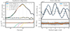 |
Fig. 3. Performance of the combined estimator on a noiseless mock catalog with ≈3.1 × 10⁶ ellipticities on a 100 deg2 area. In the upper panels, solid lines indicate the real part of the 3PCF, while dashed lines represent the imaginary part. Left-hand side: Comparison of various discrete, grid-based estimators, and a combined implementation of the multipole estimator for equilateral configurations of the zeroth natural component of the shear 3PCF. The timings correspond to the runtime on eight CPU cores and the dashed vertical lines indicate the regions of constant grid resolution for the combined estimator. In the bottom panel, we show the ratios of the real parts between all approximate implementations and the discrete estimator. The gray-shaded region displays a one-percent interval. We note that, by construction, the curve corresponding to the combined estimator always lies on top of the curve corresponding to the resolution, Δd, in the interval 20Δd ≤ Θlow ≤ Θup ≤ 40Δd. Right-hand side: Comparison of the discrete and the combined estimator for different triangle shapes. We fix two triangle sides and vary the enclosing angle, ϕ. In the bottom panel, the thick red line shows the difference between the real part of both estimators, normalized by the largest value of the discrete estimator for the given radial bin combination, maxD. The gray lines display the corresponding ratios of all other radial bin combinations, where again the normalization was done with respect to the largest value of the discrete estimator for the corresponding radial bin combination. |
To assess the accuracy of the blocks in the (Θ1, Θ2) plane shown in Fig. 2, in which the first scale was evaluated using the discrete prescription, while the second scale uses the grid-based approximation, we picked one such combination of radial bins and then varied the enclosed angle, ϕ, between them. For the example shown in the right-hand panel in Fig. 3, we chose a scale for which the Gn(Δ) are evaluated on a grid with Δ = 1′ and we find an excellent agreement between the two methods. We also show the ratios between the two schemes for all other bin combinations. Although for the majority of the curves the ratio is very close to unity, there do appear to be some spikes at which the relative difference between both estimators is at the five percent level. However, those bin configurations correspond to cases in which are only a few triplets present, and therefore they will not carry significant signal-to-noise (S/N) in realistic data with non-vanishing shape noise.
4.2. Comparison with TREECORR
The state-of-the-art method of computing shear correlation functions is based on tree codes – the most well-known implementation is the publicly available code TREECORR (Jarvis et al. 2004)7. In it, the  are estimated by explicitly accounting for all triplets. For an efficient evaluation, TREECORR first organizes the data into a hierarchical ball-tree structure from which the 3PCF is then computed. A further speedup can be achieved when allowing the bin edges to be fuzzy. For reasonable values of the associated bin_slop parameter, this approximation does not bias the mean, but does increase the measurement uncertainty (Secco et al. 2022). For an efficient binning of triangle shapes, TREECORR uses the quantities (r, u, v), which are related to the three triangle side lengths, d1 ≥ d2 ≥ d3, as
 (42)
(42)
such that with u ∈ [0, 1], v ∈ [ − 1, 1] all triangle configurations with d1 ≥ d2 ≥ d3 are covered. As is shown in Jarvis et al. (2004), this coverage is sufficient to obtain integrated measures of the 3PCF, such as the third-order aperture mass.
In Fig. 4, we compare the estimated components of the first two natural components,  , in a single noiseless mock catalog of the SLICS ensemble. For this, we first transformed the bin centers of the (Θ1, Θ2, ϕ) basis in the (r, u, v) basis and chose the value of the TREECORR measurement within the bin that the transformed bin center fell into. In order to facilitate an accurate matching between the two binning parameterizations, one needs to use very fine bins for both estimators. For our test, we computed the 3PCF between 5′ and 50′, where for the multipole-based estimator we used 40 logarithmically spaced radial bins without making use of the grid-based approximation. For the TREECORR measurement, we chose the same r binning and used 20 (40) linearly spaced bins covering the maximum range of the u (v) parameters. To achieve a reasonable run time, we only selected every tenth galaxy, leaving a total of ≈3.1 × 10⁵ ellipticities. The associated measurements were carried out on 16 CPU cores and took ≈1.5 minutes for the discrete multipole-based estimator and ≈164 minutes for TREECORR when using a value of 0.8 for the bin_slop parameter. In Fig. 4, we find good agreement overall between both estimators across the different triangle configurations; the only significant differences are visible for strongly squeezed and folded triangles. We note that the small-scale wiggles visible in the TREECORR measurements are due to the different binning parameterizations and do not reflect an additional noise component in the estimator (see Appendix B for further details).
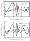 |
Fig. 4. First two natural components of the shear 3PCF on a catalog with ≈3.1 × 10⁵ shapes on a 100 deg2 area. We fixed two triangle sides and varied the enclosing angle, ϕ. Solid lines indicate the real part of the 3PCF, while dashed lines stand for the imaginary part. The regions between the dashed black lines correspond to the intervals in which the ordering of the lengths of the triangle is constant. We note that due to the different binning parameterizations of TREECORR and our estimator, we do not expect perfect agreement between the curves. |
Besides the significantly lower computational cost compared to the tree code, the multipole-based estimator also automatically allows for a fine ϕ binning of the shear 3PCF, and thus provides a good approximation even for strongly degenerate triangles8. Finally, we note that the relative speedup with respect to TREECORR increases when the combined estimator is employed and when the number density of galaxies increases. For a thorough scaling analysis of the combined estimator, we again refer to Appendix A.
5. Application to third-order aperture mass measures
Due to the large size of a data vector built from an estimate of the shear 3PCF, it is unfeasible to perform a cosmological analysis using this probe. The preferred statistic is the third-order aperture mass, which provides both a compression of the data vector and a separation of the third-order shear signal in its E- and B-modes.
5.1. Aperture mass
The aperture mass introduced in Kaiser (1995), Schneider (1996) is a measure for the projected overdensity within a circular region of radius θ around a particular location, ϑ:
 (43)
(43)
where the filter function, Uθ, is compensated, meaning that aperture mass measures evade the mass-sheet degeneracy (Falco et al. 1985). Within the flat-sky approximation, the aperture mass can also be written as the real part of a complex aperture measure, being defined in terms of the shear,
 (44)
(44)
in which Qθ is another filter function uniquely related to the choice of the Uθ filter, and φ′ denotes the polar angle of the separation vector, ϑ′. With the aperture measure being able to separate the shear signal into its E- and B-modes, it can be used for both gaining cosmological information and pinning down potential systematics. For this work, we used the exponential filter introduced in Crittenden et al. (2002),
![Mathematical equation: $$ \begin{aligned} Q_\theta (\vartheta ) = \frac{\vartheta ^2}{4\pi \theta ^4}\exp \left[\left(-\frac{\vartheta ^2}{2\theta ^2}\right)\right] \ . \end{aligned} $$](/articles/aa/full_html/2024/09/aa47987-23/aa47987-23-eq63.gif) (45)
(45)
5.2. Third-order aperture mass measures
The E/B decomposition also extends to the third-order aperture mass measures. For example, combining three aperture measures as
 (46)
(46)
one can see from Eq. (43) that the resulting quantity depends on the third-order correlation function of the convergence field. By writing down the nonredundant products that appear when combining three complex measures, ℳ, one obtains four real-valued quantities ⟨ℳap3⟩, ⟨ℳap2ℳ×⟩, ⟨ℳapℳ×2⟩, and ⟨ℳ×3⟩, which are all related to a filtered version of the third-order shear correlator. Of those, only ⟨ℳap3⟩ carries cosmological information, while the two measures, ⟨ℳap2ℳ×⟩ and ⟨ℳ×3⟩, vanish for parity symmetric shear fields (Schneider 2003), and a statistically significant signal of ⟨ℳapℳ×2⟩ indicates the presence of B-modes (Schneider et al. 2005, hereafter SKL05). Using the centroid projection Eq. (10) for the natural components, SKL05 derived an explicit form of the transformation between the Γμcen and the third-order aperture mass measures that are defined in terms of two third-order correlators of the complex aperture measure, ℳ:
 (47)
(47)
where the filter functions, F0, 1, in our convention only differ from the ones in SKL05 by cyclic permutations of the indices9. We give the explicit expressions of the filters in our convention in Appendix D.
While these two correlators are sufficient for the theoretical conversion, this might not be the case when the shear 3PCF is estimated from noisy data that is distributed over several tomographic redshift bins. In this case, one needs to include two additional correlators if the full S/N has to be retrieved:
 (48)
(48)
The individual third-order aperture mass measures then follow by a linear combination of the previous quantities; in particular, for ⟨ℳap3⟩, one has
![Mathematical equation: $$ \begin{aligned}&\left\langle {\mathcal{M} _{\mathrm{ap} }^3}\right\rangle (\theta _1,\theta _2,\theta _3) \nonumber \\&\quad \quad =\mathfrak{R} [\left\langle \mathcal{M} ^2 \mathcal{M} ^*\right\rangle (\theta _1,\theta _2,\theta _3)+\left\langle \mathcal{M} \mathcal{M} ^* \mathcal{M} \right\rangle (\theta _1,\theta _2,\theta _3) \nonumber \\&\quad \quad \quad +\left\langle \mathcal{M} ^*\mathcal{M} ^2\right\rangle (\theta _1,\theta _2,\theta _3)+\left\langle \mathcal{M} ^3\right\rangle (\theta _1,\theta _2,\theta _3)]/4 \ , \end{aligned} $$](/articles/aa/full_html/2024/09/aa47987-23/aa47987-23-eq67.gif) (49)
(49)
and the linear combinations of the remaining aperture measures can be constructed in a similar fashion.
For a tomographic setup, the structure of the equations above remains equal, but we make the substitution
 (50)
(50)
where the Γμcent(ϑ1, ϑ2, ϕ; Z1, Z2, Z3) are estimated using the method described in Sect. 3.5. This in turn means that all the other quantities, like ⟨ℳ3⟩ or ⟨ℳap3⟩, also become functions of the tomographic redshift bin combination (Z1, Z2, Z3). We note that while the third-order aperture mass is symmetric with respect to permutations in Zi, this is not the case for the shear 3PCF, and therefore one needs to average over all possible Zi permutations to obtain the full S/N. We again refer to Appendix D for all explicit expressions.
5.3. Estimators of third-order aperture measures
5.3.1. Estimation via shear 3PCF
As was established in the previous subsection, one can estimate the third-order aperture mass measures by integrating over the 3PCF on a centroid basis. To do this in practice, we first used the multipole-based estimator (Eq. 36) introduced in Sect. 3 to obtain the shear 3PCF in the × projection, then transformed them to a centroid basis via Eqs. (12–15), and finally performed the numerical integrals contained in Eq. (49). In Appendix F.2, we show the level of accuracy to which the 3PCF needs to be computed in order to guarantee a stable integration. As the computational bottleneck of this pipeline is the estimation of the shear 3PCF, the same computational speedup applies to the estimation of third-order aperture measures when using the multipole-based estimator instead of traditional estimation methods of the shear 3PCF.
5.3.2. Estimation via a direct estimator
The original estimator of the third-order aperture mass statistics in simulated data on an area, A, was introduced in Schneider et al. (1998). Instead of evaluating the statistics in terms of the shear 3PCF, it directly samples a third-order generalization of Eq. (44),
 (51)
(51)
from the ellipticities at the galaxy positions. In other words, at a particular angular position, ϑ, one has
 (52)
(52)
where we abbreviated Qθl, i ≡ Qθl(|ϑi − ϑ|) and γt, i ≡ γt(ϑi; ζi), with ϑi being the angular position of the ith galaxy and ζi denoting the direction, ϑi − ϑ. The corresponding estimate for ⟨ℳap3⟩ is then obtained by covering the survey footprint with apertures and averaging over the individual estimates. As is shown in Porth & Smith (2021), the nested sums appearing in Eq. (52) can be decomposed such that the estimation procedure scales linearly with the number of galaxies in the survey10. Although the employed Q filter (45) does formally have infinite support, one can show that by only including galaxies separated by at most 4θ from the aperture center, one recovers a practically unbiased result (Heydenreich et al. 2023). Thus, in order to avoid border effects, we do not sample apertures in regions that are separated by less than 4max(θ1, θ2, θ3) from the fields’ boundary. We recall that while the direct estimator can be used on unmasked simulated data, like the SLICS ensemble, this is not the case for real data with a nontrivial angular survey mask.
5.4. Comparison of both estimators
We compared the results of both estimation procedures on the SLICS ensemble, using all 819 mock catalogs. We first estimated the 3PCF in the interval ![Mathematical equation: $ [0{{\overset{\prime}{.}}}3125, 160{\prime}] $](/articles/aa/full_html/2024/09/aa47987-23/aa47987-23-eq71.gif) using a logarithmic bin width of
using a logarithmic bin width of  . We then transformed the 3PCF to the equal-scale aperture statistics, where for the aperture radii we chose 30 logarithmically spaced values between [1′,25′]. Finally, we estimated ⟨ℳap3⟩ using the direct estimator (52) for the same set of aperture radii. In Fig. 5, we show the measurements obtained from both estimators, together with their standard deviation across the SLICS ensemble. We find a percent-level agreement on aperture scales between 2′ and 10′. While for smaller aperture radii, the multipole-based estimator begins to yield systematically lower results, for larger aperture radii there appears to be a scatter around the zero axis. Both of these cases were expected. On the one hand, as the shear 3PCF has not been estimated down to zero separation, the integral transformation (47) cannot be fully sampled for small aperture radii. Shi et al. (2014) have demonstrated that this results in a systematic underprediction of the estimated ⟨ℳap3⟩ for aperture radii of less than ∼5 times the smallest angular separation considered in the 3PCF. At large scales, on the other hand, one would not expect both estimators to perfectly agree with each other. Cutting off the survey boundary for the direct estimator implies that both estimators do not use the data in the same way. This can also be seen in the standard deviation of both estimators across the ensemble. While for small aperture radii the error bars are of a similar size, the multipole-based estimator gradually extracts more S/N compared to the direct estimator for increasing aperture radii, as not all triangles can be accounted for in the latter due to the restricted sampling domain of the apertures.
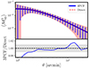 |
Fig. 5. Comparison of the third-order aperture mass statistics between the multipole-based estimator (blue line with error bars) and the direct estimator (dashed red line with error band) in the SLICS ensemble. In the lower panel, we plot the ratio between the two measurements (blue line) and show a one percent interval as the gray-shaded region. |
6. Application to the KiDS-1000 data
6.1. The KiDS-1000 data
For the first application of our estimator to real data, we used the gold sample of weak lensing and photometric redshift measurements from the fourth data release of the Kilo-Degree Survey (Kuijken et al. 2019; Wright et al. 2020; Hildebrandt et al. 2021; Giblin et al. 2021)11. The gold sample consists of around 21 million galaxies distributed over an area of 1006 square degrees (777 square degrees after masking) and is further divided into five tomographic redshift bins.
6.2. Covariance matrix
We obtain an estimate for the covariance matrix by using a suite of full-sky gravitational lensing simulations introduced in Takahashi et al. (2017) (hereafter the T17 ensemble). The underlying dark-matter-only N-body simulations were run on a ΛCDM cosmology with Ωm = 0.279, ΩΛ = 1 − Ωm, h = 0.7, σ8 = 0.82, and spectral index ns = 0.97. We constructed 1944 mock ellipticity catalogs from the T17 ensemble. In particular, we matched the angular positions, as well as the weights, the shape noise level per tomographic redshift bin, and the correlation between the measured ellipticities and the weights to the public KiDS-1000 ellipticity catalog (Giblin et al. 2021). We note that those specifications give rise to a different correlation structure than would be given by the SLICS ensemble, in which the galaxies are randomly placed within an unmasked area and in which each ellipticity carries an equal weight. For further details about the creation of the mocks, we refer to Burger et al. (2024).
To measure the shear 3PCF via the multipole estimator we first decomposed the survey area into 16 smaller patches. We proceeded along the lines of Appendix C to measure the 3PCF multipoles in each patch and then joined them, after which we obtained an unbiased estimate for the third-order aperture statistics. We measured the shear 3PCF in 38 angular bins in the interval ![Mathematical equation: $ [0{{\overset{\prime}{.}}}75,240{\prime}] $](/articles/aa/full_html/2024/09/aa47987-23/aa47987-23-eq73.gif) , yielding a mean logarithmic angular bin width of b ≈ 1.15. The choice of the lower bound was due to the pixelization scale of underlying shear maps in the T17 ensemble, which are given in a Healpix format with nside=8192, for which the individual pixels have a side length of
, yielding a mean logarithmic angular bin width of b ≈ 1.15. The choice of the lower bound was due to the pixelization scale of underlying shear maps in the T17 ensemble, which are given in a Healpix format with nside=8192, for which the individual pixels have a side length of  . As we show in Appendix F.2, this range of angular scales yields a numerically stable transformation of the shear 3PCF to the aperture mass measures for aperture scales between 4′ and 40′. We do not expect much additional information to be contained on larger aperture scales, as the third-order aperture mass only filters out non-Gaussian contributions to the cosmic shear field. As we aim to obtain an accurate covariance matrix for the unequal-scale aperture statistics in the non-tomographic setup, we computed the multipoles up to the thirtieth order in this case. In the tomographic case, we only considered equal aperture scales in the measurement, for which we show in Appendix F.2 that choosing nmax = 10 is sufficient. Finally, we transformed the shear 3PCF to the aperture statistics on two sets of radii, the “fine-binning set” consisting of 30 logarithmically spaced radii in the interval [4′,40′] and the “coarse-binning set” for which θ ∈ {4′,6′,8′,10′,14′,18′,22′,26′,32′,36′}. Using these configurations, the estimation of the third-order aperture measures per mock takes around 14 hours on a single CPU in the non-tomographic case, while 4.5 hours are required on 13 cores when including all 125 tomographic bin combinations for the 3PCF.
We produced mock covariance matrices for both a tomographic and a non-tomographic setup and display the resulting correlation matrices in Fig. 6. In particular, we see that the third-order aperture mass is highly correlated for radial bins of a similar angular scale. Similarly, there is a significant correlation between aperture measures being computed from different tomographic bin combinations. We used these sample correlation matrices to assess the detection significance of the third-order aperture measures in the KiDS-1000 data.
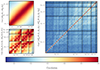 |
Fig. 6. Correlation matrices of third-order aperture mass measures in the T17 ensemble. Shown are the results for the non-tomographic, equal-scale statistics (top left), the non-tomographic unequal-scale statistics (bottom left), and the tomographic equal-scale statistics (right-hand side). We order the statistics such that θi ≤ θj ≤ θk and Z1 ≤ Z2 ≤ Z3, meaning that each of the “small” 352 squares in the covariance matrix on the right-hand side corresponds to the cross-covariance of the statistics for fixed tomographic redshift bin combinations. |
Besides the correlation structure, we have validated that there is no significant presence of B-modes in the mock catalogs and that the measurement of the E-mode matches the theoretical model introduced in Heydenreich et al. (2023). We refer to Appendix E for the corresponding figure.
6.3. Measurement results
In this subsection, we present our measurement of the third-order aperture measures in the KiDS-1000 data. Throughout this subsection, we make repeated use of the “chi-square”
![Mathematical equation: $$ \begin{aligned} \chi ^2 = \left[\mathbf{m{(\Theta )} -\mathbf d }\right]^T \mathrm{Cov} ^{-1}\left[\mathbf{m{(\Theta )} -\mathbf d }\right] \ , \end{aligned} $$](/articles/aa/full_html/2024/09/aa47987-23/aa47987-23-eq75.gif) (53)
(53)
in which d denotes the data vector, Cov stands for the covariance matrix of d, and m(Θ) is a model vector described by a set of parameters, Θ. As the covariance matrix is itself estimated from the T17 ensemble, we needed to include the Hartlap factor (Anderson 2003; Hartlap et al. 2007) to obtain an unbiased estimate for the precision matrix, Cov−1. We quote the detection significance of d by virtue of its p-value associated with the null hypothesis of a vanishing signal, m(Θ) ≡ 0. Unless otherwise stated, we estimated the p-value of a statistic measured in the KiDS-1000 data by first computing the χ2 for each of the 1944 mocks and then defining p as the fraction of mocks that have a χ2 smaller than the χ2 in the real data. Finally, we introduced the S/N of a data vector by following the definition of Secco et al. (2022):
 (54)
(54)
where Nd.o.f. denotes the degrees of freedom, which for our setup is equal to the dimension of the data vector, d. For a thorough cosmological analysis of the measurements, we refer to Burger et al. (2024).
6.3.1. Non-tomographic measurement
We estimated the non-tomographic third-order aperture measures in the KiDS-1000 data with the same angular binning that was used to obtain the corresponding covariance matrix in the T17 ensemble. While the figures were done using the fine-binning set, all statistical tests were performed on the coarsely binned set of aperture radii. We further repeated the measurement using various different setups like a finer angular binning with the combined estimator, using only the discrete estimator, excluding the patch-overlap and a run using TREECORR. In all cases, we find that the measurements scatter around each other at a level of ∼10% of the surveys’ error budget at scales ≲20′, while for larger scales the scatter increases a bit between the estimates, utilizing the overlap between footprints and the estimators that do not. All conclusions drawn from each of the setups are the same as the ones presented below.
In Fig. 7, we show our measurement of the non-tomographic third-order aperture measures, out of which only ⟨ℳap3⟩ seems to be significantly different from zero. To test the null hypothesis “no cosmological ⟨ℳap3⟩ signal”, we used the p-value introduced above but calculated the χ2 using a covariance matrix that is consistent with a noise-only signal (i.e., the ⟨ℳ×3⟩ covariance matrix). In this case, we computed the p-value using the percentile-point function of the χ2 distribution, which yields a value of p = 5.7 × 10⁻²⁸, strongly rejecting the null hypothesis. Repeating this hypothesis test (but computing the p-value as was described before Eq. 54) for the remaining three modes, we find the two parity modes and the cross mode have p-values that are consistent with a non-detection; that is, p = 0.90 for ⟨ℳap2ℳ×⟩, p = 0.26 for ⟨ℳ×3⟩, and p = 0.09 for ⟨ℳapℳ×2⟩. Besides the detection significance in the noise-only case, we can also compute the p-value and the S/N of ⟨ℳap3⟩, for which we find p = 0.05 and S/N = 3.19. We list these values, as well as the values for all other setups described in this and the following subsection, in Table 1.
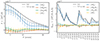 |
Fig. 7. Non-tomographic third-order aperture measures in the KiDS-1000 data, using only equal aperture scales (left) or a combination of different scales (right). The error corresponds to the standard deviation in the T17 ensemble. The solid black line compares our measurement to the mean value of the T17 ensemble and the dotted black line corresponds to the result when rescaling the measurement in the T17 ensemble to a cosmology for which the values of Ωm and S8 correspond to the best-fit values from A21. |
Detection significance of the third-order aperture measures for a range of setups.
When comparing the measured ⟨ℳap3⟩ to the mean value obtained from the T17 ensemble, we find that, while the measured ℳap3 follows a similar shape, it also has a substantially lower amplitude compared to the T17 ensemble12. The majority of this discrepancy is explained by the value of σ8 = 0.82 in the T17 ensemble, which is substantially higher than the best-fit values of σ8 measured in the KiDS-1000 data at the two-point level (Asgari et al. 2021, hereafter A21). Further, as the T17 ensemble was constructed from a set of discrete lens planes in the T17, the n(z) between the T17 ensemble and the KiDS-1000 data does slightly differ. To quantify the magnitude of these two effects, we computed the theoretical prediction using the model of Heydenreich et al. (2023) for the T17 ensemble, as well as for a setup using the KiDS-1000 n(z) and the best-fit values for Ωm ≡ 0.245 and S8 ≡ 0.759 from the KiDS-1000 analysis presented in A21. We then multiplied the measurement in the T17 ensemble with the ratio between both theory predictions and found the resulting theoretical prediction to be in agreement with our measurement in the KiDS-1000 data (p=0.54).
To measure the unequal-scale statistics displayed in the right panel of Fig. 7, we normalized the signal by θmean ≡ (θ1 θ2 θ3)1/3. We see similar features as in the measured equal-scale statistics, namely a slightly lower amplitude of the signal compared to the T17 ensemble. Again, we can strongly reject the null hypothesis of no cosmological ⟨ℳap3⟩ signal, and we also do not report a significant detection of parity-violating modes and the cross-mode. Additionally, we see that the generalized aperture statistics has a significantly higher S/N than the equal-scale statistics (S/N = 4.60). However, we note that this does not imply much tighter cosmological constraints, as the S/N measure does not take into account the dependence of the measurement on cosmological parameters. Indeed, Heydenreich et al. (2023) have demonstrated that only a little cosmological information is gained by including unequal aperture scales in a non-tomographic analysis and a similar test for a tomographic setup was carried out in Burger et al. (2024), arriving at the same conclusions. Again, our measurement can be described well by the model evaluated at the A21 cosmology (p = 0.48).
6.3.2. Tomographic measurement
Similar to the non-tomographic case, we present the measurement carried out using the same setup as for the covariance matrix. Again, choosing a different setup for the 3PCF computation, we draw the same conclusions. Due to computational constraints, we performed the measurement using TREECORR on only a few tomographic bin combinations, all of which yield consistent results.
Our measurement results for the 35 nonredundant tomographic bin combinations are shown in Fig. 8. Besides the measurement, we also show the statistical uncertainty for each aperture measure, where we note that the uncertainties for ⟨ℳap2ℳ×⟩ and ⟨ℳapℳ×2⟩ are equal to each other. As was expected, the ⟨ℳap3⟩ measurements are noise-dominated for combinations of low-redshift bins, while for higher mean redshifts the signal is significantly different from zero.
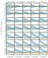 |
Fig. 8. Tomographic third-order aperture mass statistics in the KiDS-1000 data. In each panel, we show the measured statistics for a particular set of tomographic bins. The ℳap3 signal is plotted as a solid blue line, while the other solid lines indicate the remaining third-order measures. We also show the mean and the 1σ error interval for the third-order aperture mass within the T17 ensemble as a dashed blue line and a blue contour. The boundaries of the 1σ error interval for the remaining aperture measures are shown as dashed and dotted gray curves. |
To assess the detection significance of the aperture measures in the tomographic setup, we looked at the whole data vector and also performed several splits to assess potential sources of redshift-dependent systematics. In particular, we chose a data vector that only considers the auto-tomographic bin combinations, as well as a set of data vectors for which the lowest redshift bin is Zmin ∈ {2, 3, 4, 5}. In all cases, we significantly rule out the null hypothesis of a non-detection of ⟨ℳap3⟩, and we also do not find any significant signal for any of the remaining three measures. We refer to Table 1 for corresponding values.
6.3.3. Comparison to previous work
It is instructive to qualitatively compare our measurement to some previous results in the literature. Fu et al. (2014) measured the non-tomographic third-order aperture statistics in the CFHTLenS data (Heymans et al. 2012) consisting of 4.2 million galaxies and a cosmological analysis has been carried out in Simon et al. (2015). Compared to our results, they do find their measured ⟨ℳap3⟩ signal to be in rough agreement with their mock catalogs on scales ≲ 10′. Although the error budget of the CFHTLenS survey is substantially larger than the one of KiDS-1000, they also observe a dip-like feature of the ⟨ℳap3⟩ signal at larger scales. They further report a significant level of ⟨ℳapℳ×2⟩ in their measurement.
The most recent measurement of ⟨ℳap3⟩ was carried out on the Y3 ellipticity catalog of the Dark Energy Survey, consisting of roughly 100 million galaxies (Secco et al. 2022). When comparing their non-tomographic measurement to a noiseless mock catalog constructed from one of the T17 simulations, they do not observe a dip-like feature but find a strongly depleted signal of ℳap3 relative to the mock on aperture scales of less than 10′. While they do not detect a significant value of ⟨ℳapℳ×2⟩, one can see in their Fig. 3 a similar behavior of the ⟨ℳapℳ×2⟩ mode on scales between 10′ and 20′, as in our measurement.
7. Conclusions
In this work, we presented and validated a novel estimator for the natural components of the third-order shear correlation functions and applied it to the KiDS-1000 data.
Our estimator extends the work of Slepian & Eisenstein (2015), and it builds on a multipole decomposition of the shear 3PCF for which a quadratic time complexity can be achieved when projecting the natural components of the shear 3PCF in a specific way, which we dub the × basis. We further introduced a grid-based approximation, in which the ellipticity catalog is mapped onto a regular grid, for which the 3PCF multipoles can be computed via FFT methods. We then merged both prescriptions in a “combined estimator” that uses the exact computation for small angular scales, while for larger scales a grid-based approximation was employed. After including the impact of non-uniformly distributed data in the estimator, we extended the previously derived equations to a tomographic setup. We then validated our estimator and checked the applicability of the grid-based approximation to the SLICS simulation suite, finding that the grid-based approximation can be safely used for angular separations of at least 20 times the pixel scale. We furthermore compared our estimator against the state-of-the-art estimation method, TREECORR, and found an excellent agreement between both approaches, with the multipole-based approach providing a speedup of several orders of magnitude. Following a short review of how to numerically obtain the third-order aperture measures from the shear 3PCF, we validated our numerical implementation of this transformation against the direct estimator, finding a sub-percent-level agreement when using a logarithmic radial bin width, b = 1.05, in the 3PCF estimation.
Next, we proceeded to measure the third-order aperture measures in the KiDS-1000 data. We constructed a suite of 1944 mock ellipticity catalogs from the T17 ray-tracing simulations, from which we computed a sample covariance matrix that includes the effect of the KiDS-1000 footprint, the angular distribution of the galaxies, and the correlation between the galaxy weights and the measured shapes. For the non-tomographic analysis, we reported a significant detection of a cosmological ⟨ℳap3⟩ signal and also found that the parity-violating modes, as well as the cross mode, were consistent with a non-detection. For the tomographic analysis, we again report a significant detection of the ⟨ℳap3⟩ signal, while none of the remaining three modes had a suspiciously low p-value. Finally, we qualitatively compared our measurement results against previous measurements in the CFHTLenS and the DES-Y3 data.
We have demonstrated that a multipole-based estimator of the shear 3PCF provides accurate results in a fraction of the time of state-of-the-art estimation procedures. This will make it feasible to utilize these methods to measure a third-order signal in forthcoming stage-IV surveys and to construct an accurate numerical covariance matrix, taking into account all survey specifics. Extensions of these methods to higher orders are conceptually straightforward though technically cumbersome, and we leave them to future work.
We note that our definition of the Γμ[BOLD]𝒫 is different from the one found in Schneider & Lombardi (2003), but instead matches the configuration of the third-order correlators introduced in Jarvis et al. (2004) and the TREECORR implementation.
In this work, we assume that the measured ellipticity of a galaxy provides an unbiased, albeit noisy, estimate of the underlying shear field at the galaxies’ angular position.
In our implementation we use a spatial hashing data structure, as shown i.e. in Porth & Smith (2021) this method does indeed scale as 𝒪(1).
As an example, the exponential factors appearing in the Gn and Wn consist of 2n extrema, such that for a radial bin with lower bound Θlow galaxies separated by d ≪ Θlow/n will give similar contributions for the first n multipoles.
If we assume the 3PCF to not rapidly vary over small angular scales, we expect the amplitude of the 𝒩n to approach zero for large multipoles, n. Choosing a sufficiently large nmax then implies that the quantity, 𝒩ℓ − n, will have its largest contributions for n ≈ ℓ.
As we define the edges of the angular bins to always contain {20Δd, 40Δd} for all resolution scales, we do not need to consider edge cases like Θlow ≤ 40ΔΘup. We note that while these bounds are not hard-coded, we will use them for the remainder of this work whenever making use of the combined estimator.
For the tests presented in this subsection we are using version 4.2.9.
We recall that while the angular binning can be made arbitrarily small, the angular scale of the smallest features in the estimated 3PCF depends on the largest considered multipole nmax.
The origin of the permutation relative to the equations in SKL05 lies in the different conventions of the defining correlators of the Γμ in Eq. (4). This only affects the F1 filter, as the F0 filter is symmetric under permutations of the q-vectors.
We note that, as the direct estimator assumes the apertures to be fully contained within the survey footprint, its application to a nontrivial survey geometry is not easily possible.
The KiDS data products are public and available through https://kids.strw.leidenuniv.nl/DR4/
We note that in the KiDS-North patch there is a relatively strong depletion of the signal on intermediate aperture scales θ ∈ [10′,20, ]. This also translates to the analysis of the full dataset, resulting in the dip-like feature on those aperture scales visible in Fig. 7.
In this subsection we only mention contributions to the time- and space complexity that can become dominant for a given survey and measurement setup.
In our implementation the pre-factor is slightly larger than 0.25 as for each resolution scale we filter out empty pixels, guaranteeing that Npix(Δ1) ≤ Ngal for any resolution scale.
For example, for nmax = 30, nz = 5,  and a cumulative sum of reduced pixels
  of order 106 one finds, after restoring constant pre-factors, a memory requirement of ≈4.7 × 10⁹ complex-valued entries.
In order to minimize the curved-sky effects we construct the individual patches to have a rectangular shape with each side having a length of ≤10°.
We note that as the ellipticity data in the T17 ensemble itself is pixelized on a grid with a side length of ≈ 0.4′, the measurements of ⟨ℳap3⟩ are biased low for small aperture scales, independent of the smallest separation considered in the 3PCF.
Acknowledgments
We thank the anonymous referee for useful comments. This paper went through the KiDS review process, where we want to thank the KiDS internal reviewer and Joachim Harnois-Déraps for useful comments. The figures in this work were created with MATPLOTLIB (Hunter 2007) Some of the results in this paper have been derived using the healpy and HEALPix (currently http://healpix.sourceforge.net) package (Górski et al. 2005; Zonca et al. 2019). We further make use of the NUMPY (Harris et al. 2020) and SCIPY (Virtanen et al. 2020) software packages. LP acknowledges support from the DLR grant 50QE2002. SH is supported by the U.D Department of Energy, Office of Science, Office of High Energy Physics under Award Number DE-SC0019301. LL is supported by the Austrian Science Fund (FWF) [ESP 357-N]. We acknowledge use of the lux supercomputer at UC Santa Cruz, funded by NSF MRI grant AST 1828315. Author contributions: All authors contributed to the development and writing of this paper. Some results in this paper are based on observations made with ESO Telescopes at the La Silla Paranal Observatory under programme IDs 177.A-3016, 177.A-3017, 177.A-3018 and 179.A-2004, and on data products produced by the KiDS consortium. The KiDS production team acknowledges support from: Deutsche Forschungsgemeinschaft, ERC, NOVA and NWO-M grants; Target; the University of Padova, and the University Federico II (Naples).
References
- Amon, A., Gruen, D., Troxel, M. A., et al. 2022, Phys. Rev. D, 105, 023514 [NASA ADS] [CrossRef] [Google Scholar]
- Anderson, T. 2003, An Introduction to Multivariate Statistical Analysis. Wiley Series in Probability and Statistics (Wiley) [Google Scholar]
- Asgari, M., Lin, C.-A., Joachimi, B., et al. 2021, A&A, 645, A104 [NASA ADS] [CrossRef] [EDP Sciences] [Google Scholar]
- Bartelmann, M., & Schneider, P. 2001, Phys. Rep., 340, 291 [Google Scholar]
- Barthelemy, A., Codis, S., Uhlemann, C., Bernardeau, F., & Gavazzi, R. 2020, MNRAS, 492, 3420 [Google Scholar]
- Bernardeau, F., Mellier, Y., & van Waerbeke, L. 2002, A&A, 389, L28 [NASA ADS] [CrossRef] [EDP Sciences] [Google Scholar]
- Boyle, A., Uhlemann, C., Friedrich, O., et al. 2021, MNRAS, 505, 2886 [NASA ADS] [CrossRef] [Google Scholar]
- Burger, P. A., Porth, L., Heydenreich, S., et al. 2024, A&A, 683, A103 [NASA ADS] [CrossRef] [EDP Sciences] [Google Scholar]
- Chen, G., & Szapudi, I. 2005, ApJ, 635, 743 [NASA ADS] [CrossRef] [Google Scholar]
- Crittenden, R. G., Natarajan, P., Pen, U.-L., & Theuns, T. 2002, ApJ, 568, 20 [NASA ADS] [CrossRef] [Google Scholar]
- Dalal, R., Li, X., Nicola, A., et al. 2023, Phys. Rev. D, 108, 123519 [CrossRef] [Google Scholar]
- de Jong, J. T. A., Verdoes Kleijn, G. A., Erben, T., et al. 2017, A&A, 604, A134 [NASA ADS] [CrossRef] [EDP Sciences] [Google Scholar]
- Dodelson, S. 2017, Gravitational Lensing (Cambridge University Press) [CrossRef] [Google Scholar]
- Falco, E. E., Gorenstein, M. V., & Shapiro, I. I. 1985, ApJ, 289, L1 [Google Scholar]
- Fu, L., Kilbinger, M., Erben, T., et al. 2014, MNRAS, 441, 2725 [Google Scholar]
- Gatti, M., Chang, C., Friedrich, O., et al. 2020, MNRAS, 498, 4060 [Google Scholar]
- Giblin, B., Heymans, C., Asgari, M., et al. 2021, A&A, 645, A105 [NASA ADS] [CrossRef] [EDP Sciences] [Google Scholar]
- Giblin, B., Cai, Y.-C., & Harnois-Déraps, J. 2023, MNRAS, 520, 1721 [NASA ADS] [CrossRef] [Google Scholar]
- Górski, K. M., Hivon, E., Banday, A. J., et al. 2005, ApJ, 622, 759 [Google Scholar]
- Hamana, T., Takada, M., & Yoshida, N. 2004, MNRAS, 350, 893 [NASA ADS] [CrossRef] [Google Scholar]
- Hamana, T., Shirasaki, M., Miyazaki, S., et al. 2020, PASJ, 72, 16 [Google Scholar]
- Harnois-Déraps, J., Amon, A., Choi, A., et al. 2018, MNRAS, 481, 1337 [Google Scholar]
- Harnois-Déraps, J., Martinet, N., Castro, T., et al. 2021, MNRAS, 506, 1623 [CrossRef] [Google Scholar]
- Harris, C. R., Millman, K. J., van der Walt, S. J., et al. 2020, Nature, 585, 357 [NASA ADS] [CrossRef] [Google Scholar]
- Hartlap, J., Simon, P., & Schneider, P. 2007, A&A, 464, 399 [NASA ADS] [CrossRef] [EDP Sciences] [Google Scholar]
- Heydenreich, S., Brück, B., Burger, P., et al. 2022, A&A, 667, A125 [NASA ADS] [CrossRef] [EDP Sciences] [Google Scholar]
- Heydenreich, S., Linke, L., Burger, P., & Schneider, P. 2023, A&A, 672, A44 [NASA ADS] [CrossRef] [EDP Sciences] [Google Scholar]
- Heymans, C., Van Waerbeke, L., Miller, L., et al. 2012, MNRAS, 427, 146 [Google Scholar]
- Heymans, C., Grocutt, E., Heavens, A., et al. 2013, MNRAS, 432, 2433 [Google Scholar]
- Hikage, C., Oguri, M., Hamana, T., et al. 2019, PASJ, 71, 43 [Google Scholar]
- Hildebrandt, H., Viola, M., Heymans, C., et al. 2017, MNRAS, 465, 1454 [Google Scholar]
- Hildebrandt, H., van den Busch, J. L., Wright, A. H., et al. 2021, A&A, 647, A124 [EDP Sciences] [Google Scholar]
- Hou, J., Slepian, Z., & Cahn, R. N. 2023, MNRAS, 522, 5701 [NASA ADS] [CrossRef] [Google Scholar]
- Hunter, J. D. 2007, Comput. Sci. Eng., 9, 90 [NASA ADS] [CrossRef] [Google Scholar]
- Ivezić, Ž., Kahn, S. M., Tyson, J. A., et al. 2019, ApJ, 873, 111 [Google Scholar]
- Jain, B., & Seljak, U. 1997, ApJ, 484, 560 [Google Scholar]
- Jarvis, M., Bernstein, G., & Jain, B. 2004, MNRAS, 352, 338 [Google Scholar]
- Kaiser, N. 1995, ApJ, 439, L1 [Google Scholar]
- Kilbinger, M. 2015, Rep. Prog. Phys., 78, 086901 [Google Scholar]
- Kilbinger, M., & Schneider, P. 2005, A&A, 442, 69 [NASA ADS] [CrossRef] [EDP Sciences] [Google Scholar]
- Kilbinger, M., Bonnett, C., & Coupon, J. 2014, Astrophysics Source Code Library [record ascl:1402.026] [Google Scholar]
- Kratochvil, J. M., Lim, E. A., Wang, S., et al. 2012, Phys. Rev. D, 85, 103513 [Google Scholar]
- Kruse, G., & Schneider, P. 1999, MNRAS, 302, 821 [Google Scholar]
- Kuijken, K., Heymans, C., Dvornik, A., et al. 2019, A&A, 625, A2 [NASA ADS] [CrossRef] [EDP Sciences] [Google Scholar]
- Laureijs, R., Amiaux, J., Arduini, S., et al. 2011, ArXiv e-prints [arXiv:1110.3193] [Google Scholar]
- Li, X., Zhang, T., Sugiyama, S., et al. 2023, Phys. Rev. D, 108, 123518 [CrossRef] [Google Scholar]
- Linke, L., Heydenreich, S., Burger, P. A., & Schneider, P. 2023, A&A, 672, A185 [NASA ADS] [CrossRef] [EDP Sciences] [Google Scholar]
- Mandelbaum, R. 2018, ARA&A, 56, 393 [Google Scholar]
- Parroni, C., Cardone, V. F., Maoli, R., & Scaramella, R. 2020, A&A, 633, A71 [NASA ADS] [CrossRef] [EDP Sciences] [Google Scholar]
- Patton, K., Blazek, J., Honscheid, K., et al. 2017, MNRAS, 472, 439 [Google Scholar]
- Philcox, O. H. E. 2022, Phys. Rev. D, 106, 063501 [NASA ADS] [CrossRef] [Google Scholar]
- Philcox, O. H. E., Slepian, Z., Hou, J., et al. 2022, MNRAS, 509, 2457 [Google Scholar]
- Porth, L., & Smith, R. E. 2021, MNRAS, 508, 3474 [NASA ADS] [CrossRef] [Google Scholar]
- Pyne, S., & Joachimi, B. 2021, MNRAS, 503, 2300 [NASA ADS] [CrossRef] [Google Scholar]
- Schneider, P. 1996, MNRAS, 283, 837 [Google Scholar]
- Schneider, P. 2003, A&A, 408, 829 [NASA ADS] [CrossRef] [EDP Sciences] [Google Scholar]
- Schneider, P., & Lombardi, M. 2003, A&A, 397, 809 [NASA ADS] [CrossRef] [EDP Sciences] [Google Scholar]
- Schneider, P., van Waerbeke, L., Jain, B., & Kruse, G. 1998, MNRAS, 296, 873 [NASA ADS] [CrossRef] [Google Scholar]
- Schneider, P., Kilbinger, M., & Lombardi, M. 2005, A&A, 431, 9 [NASA ADS] [CrossRef] [EDP Sciences] [Google Scholar]
- Secco, L. F., Jarvis, M., Jain, B., et al. 2022, Phys. Rev. D, 105, 103537 [NASA ADS] [CrossRef] [Google Scholar]
- Semboloni, E., Heymans, C., van Waerbeke, L., & Schneider, P. 2008, MNRAS, 388, 991 [NASA ADS] [CrossRef] [Google Scholar]
- Semboloni, E., Schrabback, T., van Waerbeke, L., et al. 2011, MNRAS, 410, 143 [Google Scholar]
- Shi, X., Joachimi, B., & Schneider, P. 2014, A&A, 561, A68 [NASA ADS] [CrossRef] [EDP Sciences] [Google Scholar]
- Simon, P., Semboloni, E., van Waerbeke, L., et al. 2015, MNRAS, 449, 1505 [NASA ADS] [CrossRef] [Google Scholar]
- Slepian, Z., & Eisenstein, D. J. 2015, MNRAS, 454, 4142 [NASA ADS] [CrossRef] [Google Scholar]
- Takada, M., & Jain, B. 2003, MNRAS, 340, 580 [NASA ADS] [CrossRef] [Google Scholar]
- Takahashi, R., Hamana, T., Shirasaki, M., et al. 2017, ApJ, 850, 24 [Google Scholar]
- Takahashi, R., Nishimichi, T., Namikawa, T., et al. 2020, ApJ, 895, 113 [NASA ADS] [CrossRef] [Google Scholar]
- Troxel, M. A., MacCrann, N., Zuntz, J., et al. 2018, Phys. Rev. D, 98, 043528 [Google Scholar]
- Vicinanza, M., Cardone, V. F., Maoli, R., Scaramella, R., & Er, X. 2018, Phys. Rev. D, 97, 023519 [Google Scholar]
- Virtanen, P., Gommers, R., Oliphant, T. E., et al. 2020, Nat. Methods, 17, 261 [Google Scholar]
- Wright, A. H., Hildebrandt, H., van den Busch, J. L., & Heymans, C. 2020, A&A, 637, A100 [NASA ADS] [CrossRef] [EDP Sciences] [Google Scholar]
- Zaldarriaga, M., & Scoccimarro, R. 2003, ApJ, 584, 559 [Google Scholar]
- Zhang, L. L., & Pen, U.-L. 2005, New Astron., 10, 569 [CrossRef] [Google Scholar]
- Zonca, A., Singer, L., Lenz, D., et al. 2019, J. Open Source Softw., 4, 1298 [Google Scholar]
Appendix A: Additional implementation specifics and scaling
A.1. Notation and high-level overview
In this appendix we look at the time and space complexity of the combined estimator. For the remainder of this section, we assume a patch of Ng galaxies sampled at density  across nz tomographic bins, and we furthermore assume that we are interested in measuring all multipole components, such that we can evaluate the 3PCF (Eq. 36) between the zeroth and the nmaxth multipole on nΘ radial bins. We additionally assume that we choose a strategy in which we compute the first (smallest) nΘdisc radial bins using the discrete estimator, while the remaining nΘgrid ≡ nΘ − nΘdisc radial bins are computed using the grid-based estimator with nreso resolutions, Δi ≡ 2i − 1Δ1, for which the original ellipticity catalog is mapped to Npix(Δi) non-empty pixels and for which radial bins are used at each resolution scale,
  , such that
  . For later convenience, we also define a partition of the set of discrete radii into sets of (s1, ⋯sd) subintervals of size si.
To ensure a good compromise between the time and space complexity of the estimator, we decomposed the (Θ1, Θ2) plane into several blocks, as is shown in Fig. A.1, and calculated them in the following order: For the first block (gg block) [baseline=(char.base)] shape=circle,draw,inner sep=1pt] (char) 1;, we calculated the multipoles in which both Θ bins were computed using the grid-based approximation. We then computed the second blocks (gd blocks) [baseline=(char.base)] shape=circle,draw,inner sep=1pt] (char) 2;, which consist of the multipoles for which only one of the Θ bins was computed using the grid-based approximation, while the other one used the discrete method. Since in most applications this step consumes the most memory, we subdivided this block into d subblocks [baseline=(char.base)] shape=circle,draw,inner sep=1pt] (char) 2.i; using only si elements from the discrete bins. Finally, for the third block (dd block) [baseline=(char.base)] shape=circle,draw,inner sep=1pt] (char) 3.1;, we computed the remaining multipoles using the discrete prescription and then allocated the last gd block [baseline=(char.base)] shape=circle,draw,inner sep=1pt] (char) 2.d;.
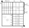 |
Fig. A.1. Decomposition of the (ϑ1, ϑ2) plane used for our implementation of the combined estimator. The grid itself is tiled into nΘ2 elements, each corresponding to a combination of angular bins (Θi, Θj), and each of those elements falls into one of the blocks, [baseline=(char.base)] shape=circle,draw,inner sep=1pt] (char) 1;, [baseline=(char.base)] shape=circle,draw,inner sep=1pt] (char) 2.i;, or [baseline=(char.base)] shape=circle,draw,inner sep=1pt] (char) 3;. |
A.2. Time complexity
For step [baseline=(char.base)] shape=circle,draw,inner sep=1pt] (char) 1;, the time complexity is of order13
![Mathematical equation: $$ \begin{aligned}&n_{\mathrm{max} } \ \ n_z \ \ \sum _{i=1}^{n_{\mathrm{reso} }} n_{\Theta ,i}^{\mathrm{grid} } \ \mathcal{O} \left[N_{\mathrm{pix} }^{(\Delta _i)} \ \log \left(N_{\mathrm{pix} }^{(\Delta _i)}\right)\right] \nonumber \\&+ \ \ n_{\mathrm{max} } \ \ n_z^3 \ \ \sum _{i=1}^{n_{\mathrm{reso} }} \left\{ \left[\left(n_{\Theta ,i}^{\mathrm{grid} }\right)^2 + 2\left(n_{\Theta ,i}^{\mathrm{grid} } \sum _{j=1}^{i-1} n_{\Theta ,j}^{\mathrm{grid} }\right)\right] \ \mathcal{O} \left(N_{\mathrm{pix} }^{(\Delta _i)}\right)\right\} \ , \end{aligned} $$](/articles/aa/full_html/2024/09/aa47987-23/aa47987-23-eq82.gif) (A.1)
(A.1)
where the terms in the first line correspond to the computation of the Gn(Δi) via FFTs and the second line concerns the time taken to average them to obtain the multipole components. In particular, the first term in the second line considers the blocks in which the resolution scales are equal, while the second term in the second line runs over all of the remaining terms contained in [baseline=(char.base)] shape=circle,draw,inner sep=1pt] (char) 1;. Noting that Npix(Δi + 1) ≈ 0.25 Npix(Δi), these expressions show the time benefit of using coarser grid resolutions for large radial separations.14 We note that both terms scale differently in the number of radial and tomographic bins; while for a coarse radial binning and a non-tomographic setup, the first term dominates, this is not true in general when the additional pre-factors in the second term surpass the additional logarithmic contribution in the first term.
The time complexity for each of the [baseline=(char.base)] shape=circle,draw,inner sep=1pt] (char) 2.i; is
 (A.2)
(A.2)
where both lines correspond to the same operations as the ones in Eq. (A.1). We note that the nmax factor in the first line is well approximated with unity, as the construction of the Gndisc in Eq. (22) only requires a single evaluation of the complex exponential from which all values for n can be inferred by a few addition and multiplication operations. We further note that between two different sub-intervals, si, sj, both terms consist of fully complementary computations, and that the second line effectively scales as if the ellipticities were distributed on regular grids.
For the first part of the final step [baseline=(char.base)] shape=circle,draw,inner sep=1pt] (char) 3;, we have
![Mathematical equation: $$ \begin{aligned} n_{\mathrm{max} } \ \left[ \ \left(\overline{n} \ \Theta _{{s}_d,\mathrm{up} }^2\right) \ \ \ + \ \ \ n_z^2 \ \ \left(n_{\Theta }^{\mathrm{disc} }\right)^2 \right] \ \mathcal{O} \left(N_{\mathrm{g} }\right) ,\end{aligned} $$](/articles/aa/full_html/2024/09/aa47987-23/aa47987-23-eq84.gif) (A.3)
(A.3)
in which both terms can be interpreted similarly to the scaling of [baseline=(char.base)] shape=circle,draw,inner sep=1pt] (char) 2.i;, but the second term is scaling only quadratically in terms of the number of z bins, as one would expect from Eq. (40).
The computation of the final gd block [baseline=(char.base)] shape=circle,draw,inner sep=1pt] (char) 2.d; is equal to the formal scaling of the second line in Eq. (A.2). We note that the first term in Eq. (A.3) is the only step in the method for which calculations are repeated, namely the allocation of the Gndisc in the interval [Θs0, low, Θsd, low]. For most realistic cases, Θsd, low ≲ 0.5 Θsd, up, meaning that the repeated calculations only constitute a subdominant fraction of the time complexity.
A.3. Space complexity
From the observation that the time complexity of the computation of the Gndisc is dominated by the computation of the first value, G1, we aim to allocate Υμ, n× for all multipole orders at once. This implies that for the allocation of the gd blocks one needs to keep all relevant GnΔi in memory - the corresponding space complexity is of the order
 (A.4)
(A.4)
Additionally, from Eq. (32) there follows the requirement to map the wγc Gndisc onto grids of corresponding pixel resolutions, which results in a memory footprint of the order
 (A.5)
(A.5)
In almost all cases, this term has the largest memory contribution,15 which leads to our subdivision of this step into d substeps requiring only 1/d-th part of the memory, while leaving the time complexity nearly untouched.
Finally, the storage requirement of the computed 3PCF multipoles is 5 (nmax + 1) nΘ2 nz3 complex-valued entries, where we made use of the symmetries
 (A.6)
(A.6)
implying that only multipoles of order n ≥ 0 need to be allocated. For our covariance setup in the T17 ensemble with nmax = 10, nΘ = 38, and nz = 5, this yields a file size of about 150 MB.
Appendix B: Parameterization of the three-point correlation function
As was stated in Sect. 4.2, the different parameterizations of the shear 3PCF for the multipole-based estimator and the TREECORR implementation prevent an exact matching of the two methods. In Fig. B.1, we compare the bin centers that were used to perform the matching in Fig. 4. We note that due to the fixed ordering of the triangles’ side lengths in TREECORR, we need to adapt the parameterization of the multipole-based estimator to the basis (d1, d2, ϕ12), where ϕ12 denotes the enclosing angle of the two largest sides, d1, d2, of the triangle.
We see that both the location and density of the bin centers are quite different between both estimators. In particular, we note that the multipole-based estimator allows for a fine binning of folded triangle configurations, while the bins corresponding to squeezed triangle configurations are more sparsely sampled. In contrast, the (r, u, v) parameterization has a dense sampling for squeezed configurations, while the folded configurations are more sparsely sampled.
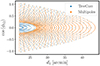 |
Fig. B.1. Distribution of bin centers for a fixed value of d2 ≈ 21.9′. We see that the TREECORR binning is finer for squeezed triangle configurations, meaning that the corresponding bin volume is smaller than that of the (Θ1, Θ2, ϕ) parameterization. |
Appendix C: Estimation on the celestial sphere
While the discussion in the main text solely focused on the efficient estimation of the shear 3PCF on a flat geometry, an actual survey will observe galaxies in the sky and will construct its ellipticity catalog, ℱ, based on a spherical topology. However, by cutting out small patches of the curved-sky catalog we can use the flat-sky approximation and apply the methods introduced in Sect. 3 to compute the shear 3PCF of each patch and then average over the individual measurements to obtain an estimate for the shear 3PCF of the full dataset.
In a more algorithmic fashion, to map a catalog on the sphere to its flat-sky analog, 𝒜, one can proceed according to the following steps:
-
Define a domain decomposition of the curved-sky catalog, ℱ, into Np smaller patches.16
-
Rotate each patch to the equator. In order to account for the different reference directions of the shapes, we made use of the angle_ref method of the healpy.Rotator class.
-
Map each rotated patch onto the flat sky using a sinusoidal projection; call these patches 𝒜i : i ∈ I ≡ {1, ⋯, Np}.
-
Define the union of the rotated and projected patches in step three as the flat-sky analog of the original catalog: ℱ ∼ 𝒜 ≡ ⋃i ∈ I𝒜i.
We are now in a position to use the methods developed in Sect. 3 to measure the correlators on the full survey footprint,  , up to the largest separation, θmax. For this, we combine the multipole components,
  , in the individual patches, 𝒜i, as follows:
 (C.1)
(C.1)
We note that, in the second step, the inner sum only runs over the Ngal, p galaxies contained in the 𝒜p, but the Gndisc are able to access data from 𝒜 - this implicit overlap of patches is necessary to account for triplets split between different patches. To implement the overlap in practice, all that needs to be done is to extend the patches to also include galaxies separated by at most θmax from the interior of each original patch, but only consider galaxies within the original patch when evaluating the inner sum in Eq. (C.1); see Fig. C.1 for an illustration.
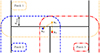 |
Fig. C.1. Counting of galaxy triplets in overlapping (extended) patches. We consider a mock footprint that is split into three patches that are extended by a scale, θmax, over their boundary. We also show three galaxies that each lie in a different patch but that are contained in the intersection of the three extended patches. When computing the 3PCF multipoles in the first patch, the form of Eq. (C.1) only allows us to compute the Gns at position x1, meaning that only the depicted triangle is included in the 3PCF. When encountering the same three galaxies in the two other patches, a different reference will be chosen, such that each particular triangle configuration will be counted sixfold across the full footprint. |
Appendix D: Transformation between shear three-point correlation function and third-order aperture measures
In this appendix, we collect the main equations that are necessary to convert a the shear 3PCF into third-order aperture measures.
D.1. Filter functions
An explicit form of the filter functions, F0 and F1, was derived in SKL05. Here, we add the equations for F2 and F3 and adapt all equations to our triangle convention. We begin by defining the helper quantities,
 (D.1)
(D.1)
 (D.2)
(D.2)
 (D.3)
(D.3)
 (D.4)
(D.4)
 (D.5)
(D.5)
 (D.6)
(D.6)
where i ∈ {1, 2, 3} and all indices should be taken mod 3. We then have for the filter functions, Fμ:
 (D.7)
(D.7)
![Mathematical equation: $$ \begin{aligned} F_1(\vartheta _1,&\vartheta _2,\phi ; \theta _1,\theta _2,\theta _3) \nonumber \\&= M \, \mathrm{e} ^{-Z} \left[ \frac{|\breve{{\boldsymbol{q}}}_1|^2|\breve{{\boldsymbol{q}}}_2|^2|\breve{{\boldsymbol{q}}}_3|^2}{24\Theta ^6}f_3^{*\, 2} f_1^{*\, 2} f_2^{2} \right. \nonumber \\&-\frac{1}{9}\frac{\breve{{\boldsymbol{q}}}_3\breve{{\boldsymbol{q}}}_1\breve{{\boldsymbol{q}}}_2^{*\,2}}{\Theta ^4} f_3^{*} f_1^{*} f_2 \, g_2^* \nonumber \\& +\frac{1}{27}\left(\frac{\breve{{\boldsymbol{q}}}_3^2 \breve{{\boldsymbol{q}}}_1^2 \breve{{\boldsymbol{q}}}_2^{*\,4}}{|\breve{{\boldsymbol{q}}}_1|^2|\breve{{\boldsymbol{q}}}_2|^2|\breve{{\boldsymbol{q}}}_3|^2 \, \Theta ^2} \, g_2^{* \, 2}\right. \nonumber \\& \left.\left. + \frac{2\theta _3^2\theta _1^2}{\Theta ^4} \ \frac{\breve{{\boldsymbol{q}}}_3\breve{{\boldsymbol{q}}}_1\breve{{\boldsymbol{q}}}_2^{*\,2}}{|\breve{{\boldsymbol{q}}}_2|^2\Theta ^2} \, f_3^* f_1^* \right)\right] \ , \end{aligned} $$](/articles/aa/full_html/2024/09/aa47987-23/aa47987-23-eq98.gif) (D.8)
(D.8)
where the  are given in (11). The other two components follow by cyclically permuting the indices in F1; that is, F2 = F1(231) and F3 = F1(312). When comparing our expressions to those in SKL05, their Fi is our Fi + 2.
D.2. Transformation into the aperture measures
By evaluating the expressions ⟨ℳ3⟩, ⟨ℳ*ℳ2⟩, ⟨ℳℳ*ℳ⟩, and ⟨ℳ2ℳ*⟩ of the complex aperture measures in terms of the (cross) aperture mass via ⟨ℳ⟩ = ⟨ℳap⟩ + i⟨ℳ×⟩, one can invert the corresponding linear system to obtain the transformation equations
![Mathematical equation: $$ \begin{aligned}&\left\langle {\mathcal{M} _{\mathrm{ap} }^3}\right\rangle (\theta _1,\theta _2,\theta _3) \nonumber \\&\quad \quad =\mathfrak{R} [\left\langle \mathcal{M} ^2 \mathcal{M} ^*\right\rangle (\theta _1,\theta _2,\theta _3)+\left\langle \mathcal{M} \mathcal{M} ^* \mathcal{M} \right\rangle (\theta _1,\theta _2,\theta _3) \nonumber \\&\quad \quad \quad +\left\langle \mathcal{M} ^*\mathcal{M} ^2\right\rangle (\theta _1,\theta _2,\theta _3)+\left\langle \mathcal{M} ^3\right\rangle (\theta _1,\theta _2,\theta _3)]/4 \ , \end{aligned} $$](/articles/aa/full_html/2024/09/aa47987-23/aa47987-23-eq100.gif) (D.9)
(D.9)
![Mathematical equation: $$ \begin{aligned}&\left\langle {\mathcal{M} _{\times }} {\mathcal{M} _{\mathrm{ap} }}^2 \right\rangle (\theta _1,\theta _2,\theta _3) \nonumber \nonumber \\&\quad = \mathfrak{I} [\left\langle \mathcal{M} ^2 \mathcal{M} ^*\right\rangle (\theta _1,\theta _2,\theta _3)+\left\langle \mathcal{M} \mathcal{M} ^* \mathcal{M} \right\rangle (\theta _1,\theta _2,\theta _3) \nonumber \\&\quad \quad - \left\langle \mathcal{M} ^*\mathcal{M} ^2\right\rangle (\theta _1,\theta _2,\theta _3)+\left\langle \mathcal{M} ^3\right\rangle (\theta _1,\theta _2,\theta _3)]/4 \ , \end{aligned} $$](/articles/aa/full_html/2024/09/aa47987-23/aa47987-23-eq101.gif) (D.10)
(D.10)
![Mathematical equation: $$ \begin{aligned}&\left\langle {\mathcal{M} _{\mathrm{ap} }} {\mathcal{M} _{\times }} {\mathcal{M} _{\mathrm{ap} }} \right\rangle (\theta _1,\theta _2,\theta _3) \nonumber \\&\quad = \mathfrak{I} [\left\langle \mathcal{M} ^2 \mathcal{M} ^*\right\rangle (\theta _1,\theta _2,\theta _3)-\left\langle \mathcal{M} \mathcal{M} ^* \mathcal{M} \right\rangle (\theta _1,\theta _2,\theta _3) \nonumber \\&\quad \quad +\left\langle \mathcal{M} ^*\mathcal{M} ^2\right\rangle (\theta _1,\theta _2,\theta _3)+\left\langle \mathcal{M} ^3\right\rangle (\theta _1,\theta _2,\theta _3)]/4 \ , \end{aligned} $$](/articles/aa/full_html/2024/09/aa47987-23/aa47987-23-eq102.gif) (D.11)
(D.11)
![Mathematical equation: $$ \begin{aligned}&\left\langle {\mathcal{M} _{\mathrm{ap} }^2} {\mathcal{M} _{\times }} \right\rangle (\theta _1,\theta _2,\theta _3) \nonumber \\&\quad = \mathfrak{I} [-\left\langle \mathcal{M} ^2 \mathcal{M} ^*\right\rangle (\theta _1,\theta _2,\theta _3)+\left\langle \mathcal{M} \mathcal{M} ^* \mathcal{M} \right\rangle (\theta _1,\theta _2,\theta _3) \nonumber \\&\quad \quad + \left\langle \mathcal{M} ^*\mathcal{M} ^2\right\rangle (\theta _1,\theta _2,\theta _3)+\left\langle \mathcal{M} ^3\right\rangle (\theta _1,\theta _2,\theta _3)]/4 \ , \end{aligned} $$](/articles/aa/full_html/2024/09/aa47987-23/aa47987-23-eq103.gif) (D.12)
(D.12)
![Mathematical equation: $$ \begin{aligned}&\left\langle {\mathcal{M} _{\mathrm{ap} }} {\mathcal{M} _{\times }^2} \right\rangle (\theta _1,\theta _2,\theta _3) \nonumber \\&\quad = \mathfrak{R} [\left\langle \mathcal{M} ^2 \mathcal{M} ^*\right\rangle (\theta _1,\theta _2,\theta _3)+\left\langle \mathcal{M} \mathcal{M} ^* \mathcal{M} \right\rangle (\theta _1,\theta _2,\theta _3) \nonumber \\&\quad \quad -\left\langle \mathcal{M} ^*\mathcal{M} ^2\right\rangle (\theta _1,\theta _2,\theta _3)-\left\langle \mathcal{M} ^3\right\rangle (\theta _1,\theta _2,\theta _3)]/4 \ , \end{aligned} $$](/articles/aa/full_html/2024/09/aa47987-23/aa47987-23-eq104.gif) (D.13)
(D.13)
![Mathematical equation: $$ \begin{aligned}&\left\langle {\mathcal{M} _{\times }} {\mathcal{M} _{\mathrm{ap} }} {\mathcal{M} _{\times }} \right\rangle (\theta _1,\theta _2,\theta _3) \nonumber \\&\quad = \mathfrak{R} [\left\langle \mathcal{M} ^2 \mathcal{M} ^*\right\rangle (\theta _1,\theta _2,\theta _3)-\left\langle \mathcal{M} \mathcal{M} ^* \mathcal{M} \right\rangle (\theta _1,\theta _2,\theta _3) \nonumber \\&\quad \quad +\left\langle \mathcal{M} ^*\mathcal{M} ^2\right\rangle (\theta _1,\theta _2,\theta _3)-\left\langle \mathcal{M} ^3\right\rangle (\theta _1,\theta _2,\theta _3)]/4 \ , \end{aligned} $$](/articles/aa/full_html/2024/09/aa47987-23/aa47987-23-eq105.gif) (D.14)
(D.14)
![Mathematical equation: $$ \begin{aligned}&\left\langle {\mathcal{M} _{\times }^2} {\mathcal{M} _{\mathrm{ap} }} \right\rangle (\theta _1,\theta _2,\theta _3) \nonumber \\&\quad = \mathfrak{R} [-\left\langle \mathcal{M} ^2 \mathcal{M} ^*\right\rangle (\theta _1,\theta _2,\theta _3)+\left\langle \mathcal{M} \mathcal{M} ^* \mathcal{M} \right\rangle (\theta _1,\theta _2,\theta _3) \nonumber \\&\quad \quad +\left\langle \mathcal{M} ^*\mathcal{M} ^2\right\rangle (\theta _1,\theta _2,\theta _3)-\left\langle \mathcal{M} ^3\right\rangle (\theta _1,\theta _2,\theta _3)]/4 \ , \end{aligned} $$](/articles/aa/full_html/2024/09/aa47987-23/aa47987-23-eq106.gif) (D.15)
(D.15)
![Mathematical equation: $$ \begin{aligned}&\left\langle {\mathcal{M} _{\times }^3} \right\rangle (\theta _1,\theta _2,\theta _3) \nonumber \\&\quad = \mathfrak{I} [\left\langle \mathcal{M} ^2 \mathcal{M} ^*\right\rangle (\theta _1,\theta _2,\theta _3)+\left\langle \mathcal{M} \mathcal{M} ^* \mathcal{M} \right\rangle (\theta _1,\theta _2,\theta _3) \nonumber \\&\quad \quad +\left\langle \mathcal{M} ^*\mathcal{M} ^2\right\rangle (\theta _1,\theta _2,\theta _3)-\left\langle \mathcal{M} ^3\right\rangle (\theta _1,\theta _2,\theta _3)]/4 \ . \end{aligned} $$](/articles/aa/full_html/2024/09/aa47987-23/aa47987-23-eq107.gif) (D.16)
(D.16)
In the main text, we averaged over the three permutations of the correlators where both, ℳap and ℳ× are present. This implies that the covariance of those components is smaller than the covariance of ⟨ℳ×3⟩.
For a tomographic setup, we need to make the adjustment that each correlator also depends on the redshift bins; in other words, we have
 (D.17)
We note that due to the symmetries of the form
 (D.18)
 (D.19)
for any π ∈ S3, the transformation equations can be reduced to the shorter expressions found, for example, in SKL05:
![Mathematical equation: $$ \begin{aligned}&\left\langle {\mathcal{M} _{\mathrm{ap} }^3}\right\rangle (\theta _1,\theta _2,\theta _3) \nonumber \\&\quad =\mathfrak{R} [\left\langle \mathcal{M} ^*\mathcal{M} ^2\right\rangle (\theta _1,\theta _2,\theta _3)+ \left\langle \mathcal{M} ^*\mathcal{M} ^2\right\rangle (\theta _1,\theta _3,\theta _2) \nonumber \\&\quad \quad +\left\langle \mathcal{M} ^*\mathcal{M} ^2\right\rangle (\theta _2,\theta _3,\theta _1)+\left\langle \mathcal{M} ^3\right\rangle (\theta _1,\theta _2,\theta _3)]/4 \ , \end{aligned} $$](/articles/aa/full_html/2024/09/aa47987-23/aa47987-23-eq111.gif) (D.20)
(D.20)
![Mathematical equation: $$ \begin{aligned}&\left\langle {\mathcal{M} _{\mathrm{ap} }^2} {\mathcal{M} _{\times }} \right\rangle (\theta _1,\theta _2,\theta _3) \nonumber \\&\quad =\mathfrak{I} [-\left\langle \mathcal{M} ^*\mathcal{M} ^2\right\rangle (\theta _1,\theta _2,\theta _3)+ \left\langle \mathcal{M} ^*\mathcal{M} ^2\right\rangle (\theta _1,\theta _3,\theta _2) \nonumber \\&\quad \quad +\left\langle \mathcal{M} ^*\mathcal{M} ^2\right\rangle (\theta _2,\theta _3,\theta _1)+\left\langle \mathcal{M} ^3\right\rangle (\theta _1,\theta _2,\theta _3)]/4 \ , \end{aligned} $$](/articles/aa/full_html/2024/09/aa47987-23/aa47987-23-eq112.gif) (D.21)
(D.21)
![Mathematical equation: $$ \begin{aligned}&\left\langle {\mathcal{M} _{\mathrm{ap} }} {\mathcal{M} _{\times }^2} \right\rangle (\theta _1,\theta _2,\theta _3) \nonumber \\&\quad =\mathfrak{R} [ \left\langle \mathcal{M} ^*\mathcal{M} ^2\right\rangle (\theta _1,\theta _2,\theta _3)+ \left\langle \mathcal{M} ^*\mathcal{M} ^2\right\rangle (\theta _1,\theta _3,\theta _2) \nonumber \\&\quad \quad -\left\langle \mathcal{M} ^*\mathcal{M} ^2\right\rangle (\theta _2,\theta _3,\theta _1)-\left\langle \mathcal{M} ^3\right\rangle (\theta _1,\theta _2,\theta _3)]/4 \ , \end{aligned} $$](/articles/aa/full_html/2024/09/aa47987-23/aa47987-23-eq113.gif) (D.22)
(D.22)
![Mathematical equation: $$ \begin{aligned}&\left\langle {\mathcal{M} _{\times }^3} \right\rangle (\theta _1,\theta _2,\theta _3) \nonumber \\&\quad =\mathfrak{I} [ \left\langle \mathcal{M} ^*\mathcal{M} ^2\right\rangle (\theta _1,\theta _2,\theta _3)+ \left\langle \mathcal{M} ^*\mathcal{M} ^2\right\rangle (\theta _1,\theta _3,\theta _2) \nonumber \\&\quad \quad +\left\langle \mathcal{M} ^*\mathcal{M} ^2\right\rangle (\theta _2,\theta _3,\theta _1)-\left\langle \mathcal{M} ^3\right\rangle (\theta _1,\theta _2,\theta _3)]/4 \ , \end{aligned} $$](/articles/aa/full_html/2024/09/aa47987-23/aa47987-23-eq114.gif) (D.23)
(D.23)
where we suppressed the redshift bin indices for better readability.
We note that if one is solely interested in the values of ⟨ℳap3⟩ and ⟨ℳ×3⟩, as well as in the averaged quantities
 (D.24)
 (D.25)
it is sufficient to only compute the 3PCF for Z1 ≤ Z2 ≤ Z3, if one uses the full transformation equations (D.9-D.16) and additionally symmetrizes them over the three aperture radii.
Appendix E: Measurements in the T17 Ensemble
Fig. E.1 displays the measurement of the third-order aperture statistics in the T17 ensemble consisting of 1944 mock ellipticity catalogs mimicking the KiDS-1000 survey. We see that most of the cosmological signal is contained in tomographic bin combinations consisting of high–z bins. However, for a cosmological analysis, one should also include the low–z bins, as those will help to constrain parameters related to the intrinsic alignment model. We also see that none of the three cross-aperture measures yields a significant signal, showing that such a spurious signal is neither present in the mock ellipticity catalogs nor created by our estimation procedure. Finally, we compare our measurement to the theoretical prediction, for which we use the model introduced in Heydenreich et al. (2023). On small angular scales, we see that the measurement does slightly overpredict the theory, which we attribute to the reduced-shear effect that is included in the T17 ensemble but not in the theory. On large angular scales, however, the measurement does slightly underpredict the theoretical prediction. One reason for this could lie in the lens-shell thickness in the T17 ensemble; in particular, Takahashi et al. (2017) show that on the level of the shear 2PCF this effect can cause a suppression in the signal of up to 10% for angular separations of about 100′. Besides these two effects, a part of the discrepancy between the theory and the measurement could also lie in the limited accuracy of the Bihalofit model (Takahashi et al. 2020), which is at the 10% level.
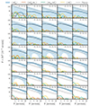 |
Fig. E.1. Tomographic third-order aperture mass statistics in the T17 ensemble. In each panel, we show the measured statistic for one configuration of the tomographic bins. The mean ℳap3 signal and its standard deviation are plotted as the solid blue line and the blue error band. The other solid lines indicate the absolute values of the remaining third-order measures and the 1σ uncertainty level of those measures are indicated by the dashed gray (dotted) lines. The theoretical prediction is shown as the dotted black line. |
Appendix F: Accuracy requirements
F.1. Three-point correlation function
In Fig. F.1 we show the detection significance of some multipoles,  , in the SLICS ensemble for noisy and noiseless data. We see that most of the signal contribution stems from the lowest-order multipoles. This was expected, as the shear 3PCF does not contain high-frequency oscillations in the φ direction. We also see that shape noise strongly depletes the detection significance of the individual elements; we note that for a stage-IV survey that has a significantly higher source density, this effect will not be as severe. The plots for the three remaining
  all follow the same trend.
F.2. Third-order aperture mass
With the third-order aperture mass being an integrated measure of the shear 3PCF for which the time and space complexity is strongly dependent on the number of radial bins and the largest considered multipole, one should investigate the convergence of the numerical integration for various binning choices. In Fig. F.2, we fix the largest multipole nmax = 20 and compare the numerical integration of the 3PCF for a range of logarithmic bin widths, b. For the equal-scale apertures, we find that choosing a value of b ≈ 1.1 yields a percent-level accuracy. This value is similar to the corresponding value found by previous studies (Fu et al. 2014; Secco et al. 2022) examining the convergence of the numerical integration using TREECORR. We further show in Fig. F.2 that our choice of b ≈ 1.15 for the computation of the numerical covariance from the T17 ensemble yields sufficiently accurate data vectors for aperture scales of more than 4′.17 For the multiscale aperture statistics, we find similar convergence properties, except for the cases when two aperture radii are considerably smaller than the third one.
In Fig. F.3, we compare how limiting the number of considered multipoles impacts the expected value of ⟨ℳap3⟩. We find, as before, a very fast convergence for the equal-scale aperture statistics, while for the general case there is a strong dependence of the level of convergence on the ratio between the two smallest and the largest aperture radii. This behavior can be understood as follows: in the case of two small and one large aperture radii, the associated ⟨ℳap3⟩ is dominated by squeezed triangle configurations. As such configurations mainly receive contributions from the multipole components, Υμ, n(Θ, Θ), and those are precisely the ones having a nonvanishing and detectable signal for large multipole orders (see Fig. F.1), we do expect a slower convergence.
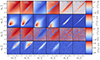 |
Fig. F.1. Mean signal and detectability of the higher-order multipoles, Υ0, n×, in the SLICS ensemble, after averaging over all 819 realizations. In the top row, we show the mean signal from the noiseless SLICS ensemble. To aid the visualization, we normalize the multipoles by the product of the corresponding angular bins and further use a logarithmic scaling for positive and negative values in the color map. In the second row, we show the S/N ratio of the modulus of the corresponding multipole component. The third and fourth rows display the same measurements when shape noise is included in the mocks. |
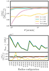 |
Fig. F.2. Accuracy of the numerical integration of the shear 3PCF to the third-order aperture statistics for different logarithmic spacings of radial bins, as well as for the radial binning that was used in the computation of the covariance in the T17 ensemble. All measurements were done in the SLICS ensemble. In the upper panel, we show the ratio between ⟨ℳap3⟩ when estimated using a particular logarithmic bin width, b, for the shear 3PCF and the corresponding result with b ≡ 1.05. In the lower panel, we show the corresponding results when allowing for unequal aperture filters. |
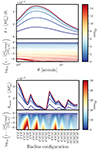 |
Fig. F.3. Impact of higher-order multipoles of the shear 3PCF on the third-order aperture statistics in the SLICS ensemble. In the upper panel of the top (bottom) figure, we show the estimated signal for the equal-scale (unequal-scale) statistics, when using only the first nmax multipoles. The lower panel displays the decimal logarithm of the fractional difference between the measurement using 50 multipoles and the measurements using only multipoles up until nmax. |
All Tables
Detection significance of the third-order aperture measures for a range of setups.
All Figures
|
Fig. 1. Upper panel: Parameterization of a triplet of shears used in this work. For some shears at position X1, we denote the connecting lines to the two other shears as ϑi and the enclosing angle as ϕ. The dashed red lines show the directions of the × projection Eq. (9) for which the three projection axes intersect in X1. Lower panel: Definition of the geometric quantities involved in the centroid projection Eq. (10). We see that the q vectors connect the centroid of the triangle with the triangles’ vertices. |
| In the text | |
|
Fig. 2. General strategy for computing the three-point correlators used in this work. For small angular scales, we used the prescription for discrete data to compute the Gn and the Υi, n×, while for larger scales, we used the grid-based approximation with varying resolution scales, Δ. For the off-diagonal elements, we first computed the Gn of each radial bin using the corresponding method and then mapped them to the grid of the larger resolution scale from which the Υi, n× were obtained. |
| In the text | |
|
Fig. 3. Performance of the combined estimator on a noiseless mock catalog with ≈3.1 × 10⁶ ellipticities on a 100 deg2 area. In the upper panels, solid lines indicate the real part of the 3PCF, while dashed lines represent the imaginary part. Left-hand side: Comparison of various discrete, grid-based estimators, and a combined implementation of the multipole estimator for equilateral configurations of the zeroth natural component of the shear 3PCF. The timings correspond to the runtime on eight CPU cores and the dashed vertical lines indicate the regions of constant grid resolution for the combined estimator. In the bottom panel, we show the ratios of the real parts between all approximate implementations and the discrete estimator. The gray-shaded region displays a one-percent interval. We note that, by construction, the curve corresponding to the combined estimator always lies on top of the curve corresponding to the resolution, Δd, in the interval 20Δd ≤ Θlow ≤ Θup ≤ 40Δd. Right-hand side: Comparison of the discrete and the combined estimator for different triangle shapes. We fix two triangle sides and vary the enclosing angle, ϕ. In the bottom panel, the thick red line shows the difference between the real part of both estimators, normalized by the largest value of the discrete estimator for the given radial bin combination, maxD. The gray lines display the corresponding ratios of all other radial bin combinations, where again the normalization was done with respect to the largest value of the discrete estimator for the corresponding radial bin combination. |
| In the text | |
|
Fig. 4. First two natural components of the shear 3PCF on a catalog with ≈3.1 × 10⁵ shapes on a 100 deg2 area. We fixed two triangle sides and varied the enclosing angle, ϕ. Solid lines indicate the real part of the 3PCF, while dashed lines stand for the imaginary part. The regions between the dashed black lines correspond to the intervals in which the ordering of the lengths of the triangle is constant. We note that due to the different binning parameterizations of TREECORR and our estimator, we do not expect perfect agreement between the curves. |
| In the text | |
|
Fig. 5. Comparison of the third-order aperture mass statistics between the multipole-based estimator (blue line with error bars) and the direct estimator (dashed red line with error band) in the SLICS ensemble. In the lower panel, we plot the ratio between the two measurements (blue line) and show a one percent interval as the gray-shaded region. |
| In the text | |
|
Fig. 6. Correlation matrices of third-order aperture mass measures in the T17 ensemble. Shown are the results for the non-tomographic, equal-scale statistics (top left), the non-tomographic unequal-scale statistics (bottom left), and the tomographic equal-scale statistics (right-hand side). We order the statistics such that θi ≤ θj ≤ θk and Z1 ≤ Z2 ≤ Z3, meaning that each of the “small” 352 squares in the covariance matrix on the right-hand side corresponds to the cross-covariance of the statistics for fixed tomographic redshift bin combinations. |
| In the text | |
|
Fig. 7. Non-tomographic third-order aperture measures in the KiDS-1000 data, using only equal aperture scales (left) or a combination of different scales (right). The error corresponds to the standard deviation in the T17 ensemble. The solid black line compares our measurement to the mean value of the T17 ensemble and the dotted black line corresponds to the result when rescaling the measurement in the T17 ensemble to a cosmology for which the values of Ωm and S8 correspond to the best-fit values from A21. |
| In the text | |
|
Fig. 8. Tomographic third-order aperture mass statistics in the KiDS-1000 data. In each panel, we show the measured statistics for a particular set of tomographic bins. The ℳap3 signal is plotted as a solid blue line, while the other solid lines indicate the remaining third-order measures. We also show the mean and the 1σ error interval for the third-order aperture mass within the T17 ensemble as a dashed blue line and a blue contour. The boundaries of the 1σ error interval for the remaining aperture measures are shown as dashed and dotted gray curves. |
| In the text | |
|
Fig. A.1. Decomposition of the (ϑ1, ϑ2) plane used for our implementation of the combined estimator. The grid itself is tiled into nΘ2 elements, each corresponding to a combination of angular bins (Θi, Θj), and each of those elements falls into one of the blocks, [baseline=(char.base)] shape=circle,draw,inner sep=1pt] (char) 1;, [baseline=(char.base)] shape=circle,draw,inner sep=1pt] (char) 2.i;, or [baseline=(char.base)] shape=circle,draw,inner sep=1pt] (char) 3;. |
| In the text | |
|
Fig. B.1. Distribution of bin centers for a fixed value of d2 ≈ 21.9′. We see that the TREECORR binning is finer for squeezed triangle configurations, meaning that the corresponding bin volume is smaller than that of the (Θ1, Θ2, ϕ) parameterization. |
| In the text | |
|
Fig. C.1. Counting of galaxy triplets in overlapping (extended) patches. We consider a mock footprint that is split into three patches that are extended by a scale, θmax, over their boundary. We also show three galaxies that each lie in a different patch but that are contained in the intersection of the three extended patches. When computing the 3PCF multipoles in the first patch, the form of Eq. (C.1) only allows us to compute the Gns at position x1, meaning that only the depicted triangle is included in the 3PCF. When encountering the same three galaxies in the two other patches, a different reference will be chosen, such that each particular triangle configuration will be counted sixfold across the full footprint. |
| In the text | |
|
Fig. E.1. Tomographic third-order aperture mass statistics in the T17 ensemble. In each panel, we show the measured statistic for one configuration of the tomographic bins. The mean ℳap3 signal and its standard deviation are plotted as the solid blue line and the blue error band. The other solid lines indicate the absolute values of the remaining third-order measures and the 1σ uncertainty level of those measures are indicated by the dashed gray (dotted) lines. The theoretical prediction is shown as the dotted black line. |
| In the text | |
|
Fig. F.1. Mean signal and detectability of the higher-order multipoles, Υ0, n×, in the SLICS ensemble, after averaging over all 819 realizations. In the top row, we show the mean signal from the noiseless SLICS ensemble. To aid the visualization, we normalize the multipoles by the product of the corresponding angular bins and further use a logarithmic scaling for positive and negative values in the color map. In the second row, we show the S/N ratio of the modulus of the corresponding multipole component. The third and fourth rows display the same measurements when shape noise is included in the mocks. |
| In the text | |
|
Fig. F.2. Accuracy of the numerical integration of the shear 3PCF to the third-order aperture statistics for different logarithmic spacings of radial bins, as well as for the radial binning that was used in the computation of the covariance in the T17 ensemble. All measurements were done in the SLICS ensemble. In the upper panel, we show the ratio between ⟨ℳap3⟩ when estimated using a particular logarithmic bin width, b, for the shear 3PCF and the corresponding result with b ≡ 1.05. In the lower panel, we show the corresponding results when allowing for unequal aperture filters. |
| In the text | |
|
Fig. F.3. Impact of higher-order multipoles of the shear 3PCF on the third-order aperture statistics in the SLICS ensemble. In the upper panel of the top (bottom) figure, we show the estimated signal for the equal-scale (unequal-scale) statistics, when using only the first nmax multipoles. The lower panel displays the decimal logarithm of the fractional difference between the measurement using 50 multipoles and the measurements using only multipoles up until nmax. |
| In the text | |
Current usage metrics show cumulative count of Article Views (full-text article views including HTML views, PDF and ePub downloads, according to the available data) and Abstracts Views on Vision4Press platform.
Data correspond to usage on the plateform after 2015. The current usage metrics is available 48-96 hours after online publication and is updated daily on week days.
Initial download of the metrics may take a while.