| Issue |
A&A
Volume 646, February 2021
|
|
|---|---|---|
| Article Number | A147 | |
| Number of page(s) | 23 | |
| Section | Cosmology (including clusters of galaxies) | |
| DOI | https://doi.org/10.1051/0004-6361/202039682 | |
| Published online | 19 February 2021 | |
The PAU Survey: Intrinsic alignments and clustering of narrow-band photometric galaxies
1
Department of Physics and Astronomy, University College London, Gower Street, London WC1E 6BT, UK
e-mail: This email address is being protected from spambots. You need JavaScript enabled to view it.
2
Institute for Theoretical Physics, Utrecht University, Princetonplein 5, 3584 CE Utrecht, The Netherlands
3
Institute for Computational Cosmology, Department of Physics, Durham University, South Road, Durham DH1 3LE, UK
4
Centre for Extragalactic Astronomy, Department of Physics, Durham University, South Road, Durham DH1 3LE, UK
5
Leiden Observatory, Leiden University, PO Box 9513, 2300 RA Leiden, The Netherlands
6
Institut de Física d’Altes Energies (IFAE), The Barcelona Institute of Science and Technology, Campus Univ. A. de Barcelona, 08193 Bellaterra, Barcelona, Spain
7
Institute of Space Sciences (ICE, CSIC), Campus UAB, Carrer de Can Magrans, s/n, 08193 Barcelona, Spain
8
Institut d’Estudis Espacials de Catalunya (IEEC), 08034 Barcelona, Spain
9
National Centre for Nuclear Research, ul. Hoza 69, 00-681 Warsaw, Poland
10
Institute for Particle Physics and Astrophysics, ETH Zürich, Wolfgang-Pauli-Str. 27, 8093 Zürich, Switzerland
11
CIEMAT, Centro de Investigaciones Energéticas, Medioambientales y Tecnológicas, Avda. Complutenes 40, 28040 Madrid, Spain
12
Instituto de Física Teórica IFT-UAM/CSIC, Universidad Autónoma de Madrid, 28049 Madrid, Spain
13
Ruhr-University Bochum, Astronomical Institute, German Centre for Cosmological Lensing, Universitätsstr. 150, 44801 Bochum, Germany
14
Institució Catalana de Recerca i Estudis Avançats (ICREA), 08010 Barcelona, Spain
15
Port d’Informació Científica (PIC), Campus UAB, C. Albareda s/n, 08193 Bellaterra, Barcelona, Spain
Received:
15
October
2020
Accepted:
30
December
2020
Abstract
We present the first measurements of the projected clustering and intrinsic alignments (IA) of galaxies observed by the Physics of the Accelerating Universe Survey (PAUS). With photometry in 40 narrow optical passbands (4500 Å–8500 Å), the quality of photometric redshift estimation is σz ∼ 0.01(1 + z) for galaxies in the 19 deg2 Canada-France-Hawaii Telescope Legacy Survey W3 field, allowing us to measure the projected 3D clustering and IA for flux-limited, faint galaxies (i < 22.5) out to z ∼ 0.8. To measure two-point statistics, we developed, and tested with mock photometric redshift samples, ‘cloned’ random galaxy catalogues which can reproduce data selection functions in 3D and account for photometric redshift errors. In our fiducial colour-split analysis, we made robust null detections of IA for blue galaxies and tentative detections of radial alignments for red galaxies (∼1 − 3σ), over scales of 0.1 − 18 h−1 Mpc. The galaxy clustering correlation functions in the PAUS samples are comparable to their counterparts in a spectroscopic population from the Galaxy and Mass Assembly survey, modulo the impact of photometric redshift uncertainty which tends to flatten the blue galaxy correlation function, whilst steepening that of red galaxies. We investigate the sensitivity of our correlation function measurements to choices in the random catalogue creation and the galaxy pair-binning along the line of sight, in preparation for an optimised analysis over the full PAUS area.
Key words: cosmology: observations / large-scale structure of Universe / gravitational lensing: weak
© ESO 2021
1. Introduction
The estimation of accurate and precise galaxy redshifts over large samples is one of the major challenges in cosmology today; studies of the evolution of large-scale structure and the expansion rate of the Universe require precise knowledge of distances, which can be difficult to obtain. High-resolution spectroscopy remains an expensive technique, which is unsuited to the large volumes explored by modern wide-field galaxy surveys. Photometric redshift (photo-z) estimation is thus an active field of development, with various foci directed towards template-fitting (with Bayesian methods, e.g., BPZ; Benitez 2000, or maximum-likelihood fitting, e.g., HyperZ; Bolzonella et al. 2000), empirical machine learning (e.g., Directional Neighbourhood Fitting with k-nearest neighbours; De Vicente et al. 2016, or combining neural networks, decision trees, and k-nearest neighbours in e.g., ANNz2; Sadeh et al. 2016), and combinations thereof (e.g., training and template-fitting with LEPHARE; Arnouts et al. 1999; Ilbert et al. 2006) – for a recent review of photo-z methods, see Salvato et al. (2019).
The Physics of the Accelerating Universe Survey (PAUS; Benítez et al. 2009) tackles the photo-z challenge with 40 narrow-band (NB) photometric filters, each 130 Å in width, with centres in steps of 100 Å from 4500 Å to 8500 Å. In combination with existing broad-band photometry, the intermediate-resolution spectra from PAUS yield up to order-of-magnitude improvements in the precision of photo-z, as compared with broad-band-only estimates (e.g., Hildebrandt et al. 2012; Martí et al. 2014; Hoyle et al. 2018; Alarcon et al. 2020).
PAUS allows us to explore hitherto uncharted astrophysical environments, namely the weakly non-linear regime of 10 − 20 h−1 Mpc over a broad redshift epoch. PAUS straddles the boundary between (i) spectroscopic surveys, with long exposures and thus accurate redshifts, over smaller areas and volumes, and (ii) broad-band photometric surveys, having short exposures and poorer-quality redshifts, but over larger areas and volumes. PAUS thus allows for a deep, dense sampling, over an intermediate area, with unprecedented photo-z precision. As such, these data offer unique snapshots of many phenomena as galaxy and small-scale processes (e.g., various feedback mechanisms, non-linear density evolution) start to prompt departures from the linear regime. Early analyses carried out for the PAU survey have included: simulations and mock catalogue generation (Stothert et al. 2018); machine learning approaches to star-galaxy classification and sky-background estimation (Cabayol et al. 2019; Cabayol-Garcia et al. 2020); forward-modelling for narrow-band imaging (Tortorelli et al. 2018); improved photometric redshift calibration (Alarcon et al. 2021; Eriksen et al. 2020); and forecasting for Ly-α intensity mapping (Renard et al. 2021), among others.
Primary science cases for PAUS include redshift-space distortions (RSD; Kaiser 1987), galaxy intrinsic alignments (IA; Heavens et al. 2000; Croft & Metzler 2000; Catelan et al. 2001; Hirata & Seljak 2004) and galaxy clustering (e.g., Zehavi et al. 2002), with secondary cases for, for example, magnification (Schmidt et al. 2012). This paper focuses on the production of tailored random galaxy catalogues for PAUS, and presents initial measurements of the projected 3D intrinsic alignments and clustering of PAUS galaxies.
We developed random galaxy catalogues following the formalism laid down by Cole (2011) and Farrow et al. (2015) in order to reproduce the radial selection function of the data, without any clustering along the line-of-sight. With these, and the photo-z precision offered by PAUS, we are able to extend measurements of projected galaxy clustering and IA into a new regime of intrinsically faint objects up to intermediate redshifts of z ≲ 1, with a particular increase in statistical power for faint, blue galaxies. Our work is complementary to other direct studies of galaxy intrinsic alignments: for example, Mandelbaum et al. (2011) made null detections of alignments for bright emission-line galaxies around z ∼ 0.6 in the WiggleZ survey (Drinkwater et al. 2010); Tonegawa et al. (2018) did the same for faint, high-redshift (z ∼ 1.4), star-forming galaxies in the FastSound survey (Tonegawa et al. 2015); as did Johnston et al. (2019) when considering blue galaxies at lower redshifts in the Galaxy and Mass Assembly (GAMA) survey – evidence continues to mount for negligible alignments in blue, spiral galaxies, going against theoretical predictions for strong alignments around the peaks of the matter distribution, which are brought on by tidal torquing mechanisms (see Schafer 2009, for a review). With the depth and high number density of PAUS, we push to smaller comoving galaxy-pair separations (Rodriguez et al. 2020) where any signal ought to be strongest, and seek to add another data-point to the picture of blue galaxy alignments in flux-limited samples.
PAUS also presents an opportunity to attempt an extension into the faint regime of the luminosity-scaling of bright red galaxy IA found by some analyses (Joachimi et al. 2011; Singh et al. 2015). Johnston et al. (2019) found no evidence for such a scaling; however, they acknowledged complications due to satellite galaxy fractions – the comprehensive work of Fortuna et al. (2021) modelled central and satellite, red and blue galaxy alignment contributions via the IA halo model (based on Schneider & Bridle 2010), finding that whilst bright red galaxies might exhibit this luminosity scaling, the faint end is relatively unconstrained. With a similar redshift baseline to the luminous red galaxies (LRGs) studied by Joachimi et al. (2011) and Singh et al. (2015), PAUS is ideally suited to assess any luminosity-dependence of IA for these fainter red galaxies, should it exist.
This paper is structured as follows; Sect. 2 describes our galaxy data from the PAUS and GAMA surveys. In Sect. 3, we detail our construction of ‘cloned’ random galaxy catalogues. We describe the methods for measuring projected statistics in Sect. 4, and discuss the results in Sect. 5. We present our concluding remarks in Sect. 6. Throughout this analysis, we quote AB magnitudes unless otherwise stated, and we compute comoving coordinates/volumes assuming a flat ΛCDM universe, with Ωm = 0.25, h = 0.7, Ωb = 0.044, ns = 0.95 and σ8 = 0.8.
2. Data
Here we provide a brief overview of the Physics of the Accelerating Universe Survey (PAUS; Benítez et al. 2009), and point readers to Eriksen et al. (2019), and references therein, for further details.
2.1. PAU Survey
PAUS is conducted at the William Herschel Telescope (WHT), at the Observatorio del Roque de los Muchachos on La Palma, with the purpose-built PAUCam (Padilla et al. 2019) instrument – the camera sports 40 narrow-band and 6 broad-band filters on interchangeable trays, with 8 narrow-bands per tray. Each pointing is observed with between 3 and 5 dithers per tray, and exposure times for each tray are adjusted to yield as close as possible to uniform signal-to-noise ratio (S/N) as a function of wavelength – in practice, with 8 NBs per tray, total uniformity cannot be achieved, and the S/N grows from the near-UV (limited by readout noise) to the near-IR (sky-limited).
This analysis uses PAUS data taken in the W3 field, targeting galaxies detected by the Canada-France-Hawaii Telescope Legacy Survey (CFHTLS; Cuillandre & Bertin 2006). The current PAUS coverage of W3 is ∼19 deg2 – the completed PAU Survey aims to cover ∼100 deg2 over several non-contiguous fields – and we retain 263 227 galaxies for analysis after imposing the flux-limit i < 22.5, and rejecting stars (see Erben et al. 2013, for CFHTLenS star_flag details) and bright sources with i < 18, and sources for which we were missing five or more narrow-bands. The PAUS W3 field footprint is displayed in Fig. 1, where galaxy points are coloured according to our photo-z quality marker Qz (lower values = better photo-z; see Sects. 2.2 and 2.6) – one sees that there are no obvious trends in photo-z quality with respect to positions on-sky. For our correlation function analysis, we reject objects for which shape estimation failed completely1, and further restrict our PAUS samples to 189 338 galaxies within the photo-z range 0.1 < zphot. < 0.8 (for reasons we discuss in Sect. 2.6).
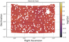 |
Fig. 1. Distribution of galaxies in the PAUS W3 field, with points coloured according to the log of each galaxy’s Qz value – this quantity describes the quality of photometric redshift estimation (low Qz = high photo-z quality) through a combination of the goodness-of-fit of SED templates to narrow-band photometry, and the shape of the resulting redshift probability density function; see Sects. 2.2 and 2.6. Circular holes in the footprint correspond to masks around foreground stars, with the largest gap (top-right) covering the Pinwheel Galaxy (Messier 101). |
2.2. BCNZ2 and k-corrections
The BCNZ2 photometric redshift algorithm – presented in detail by Eriksen et al. (2019) – was designed to tackle the challenge of photo-z estimation with 40 optical narrow-bands, supplementary broad-bands (from CFHTLS), and the flexible utilisation of galaxy emission lines – the latter point in particular is important, since many of the high-redshift, blue galaxies targeted by PAUS lack large spectral breaks. As Eriksen et al. (2019) show, strong emission lines from these galaxies can be leveraged to achieve powerfully precise photo-z – reaching accuracies of σz = 0.0037(1 + z) for the best 50% of photo-z derived for the COSMOS field. Descriptors for the quality of photo-z estimates are explored by Eriksen et al. (2019) – we make use of the Qz parameter (their Sect. 5.5) when assessing photo-z in W3, and the impacts of quality-cuts.
The method of BCNZ2 involves fitting to the narrow-band flux data with linear combinations of template galaxy SEDs (based upon Bruzual & Charlot 2003, and described in Eriksen et al. 2019; Sect. 4.4) – as a by-product of this procedure, we gain a best-fitting SED model for each object, which we can redshift arbitrarily. From these models we are able to easily compute unique k-corrections per object, for a given band, via
 (1)
(1)
where fz is the flux transmitted to the observer, in that waveband, by an object at redshift z; thus fzobs. is the observed flux of the object in that band. The k-correction kz(zobs.) then modifies the flux of a galaxy at redshift zobs. to look as though it were at redshift z; k-corrections are thus necessary to infer the maximum redshift zmax at which a galaxy can be observed by a flux-limited survey. Figure 2 displays k0(z) for PAUS W3 galaxies – these are the k-corrections from a given redshift z to z = 0. Given that k-corrections are known to correlate strongly with galaxy type (via the archetypal forms of SEDs), we also defined a set of k-corrections by binning galaxies according to their rest-frame absolute u − i colour (estimated using LEPHARE – see below), before taking running medians of k0(z) for each colour-bin (McNaught-Roberts et al. 2014) – these median k-corrections are displayed as solid lines in Fig. 2. We found however, that the colour-median and the unique (per-galaxy) corrections yielded negligibly different estimates for the redshifts zmax at which galaxies (of fixed magnitude) cross the survey flux-limit – to be discussed in Sect. 3.
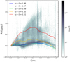 |
Fig. 2. Hexagonally-binned 2D histogram of PAUS W3 galaxies’ i-band k-corrections from redshift z (x-axis) to z = 0 – we assembled these by redshifting each galaxy’s best-fit SED model over the entire z-range, and taking ratios (Eq. (1)) of fluxes to the z = 0 flux. Cells are coloured by the count of galaxies resident in each cell. Solid coloured lines give the running-medians of k0(z) for five rest-frame colour bins, for which the average colours ⟨u − i⟩ are given in the legend (absolute magnitudes estimated with LEPHARE). |
2.3. Rest-frame magnitudes and colours
When quoting rest-frame magnitudes, or estimating PAUS W3 galaxy colours, we make use of two independent determinations of these quantities: (i) those derived for CFHTLenS galaxies (see Erben et al. 2013) using the LEPHARE (Arnouts et al. 1999; Ilbert et al. 2006) package, and (ii) those we have determined for PAUS, using the CIGALE (Noll et al. 2009; Boquien et al. 2019) software package. The former quantities were derived with low-resolution photometry and are consequently more noisy/prone to biases and degeneracies in redshift-colour space – such as those clearly visible in Fig. 3 (top-left panel). The rest-frame colours we have derived with CIGALE make use of the full complement of PAUS photometry, with 40 narrow-bands and 6 CFHTLS broad-bands, yielding smoother colour-magnitude distributions (bottom-panels). We draw a line u − i = 1.138 − 0.038i on the PAUS LEPHARE colour-magnitude plane, above which we classify galaxies as ‘red’ (early-type) with ‘blue’ (late-type) galaxies below – this boundary is fairly arbitrary, chosen only to separate a dense red sequence from the more diffuse blue cloud, each visible in the top-left panel of Fig. 3. For CIGALE colours, we have separated galaxy types using 2- or 3-cluster classifications (as described in Siudek et al. 2018a,b) in the multidimensional rest-frame colour-magnitude space: {i, g − i, r − z, g − r, u − g}, resulting in definitions for red-sequence and blue-cloud galaxy samples with some interlopers (2-cluster), or red/blue samples with theoretically greater purity, having excluded the green valley (3-cluster). We shall measure and compare correlations in PAUS with each of these three different colour classifications.
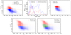 |
Fig. 3. Top-left: absolute rest-frame colour u − i vs. i magnitude for PAUS galaxies in the W3 area. These rest-frame magnitudes were derived for CFHTLenS (Erben et al. 2013) using the LEPHARE software package (Arnouts et al. 1999; Ilbert et al. 2006). We define the red sequence as those galaxies for whom u − i > 1.138 − 0.038i, as indicated by the orange line. Top-middle: spectroscopic redshift distribution of galaxies in GAMA, and photo-z distribution of PAUS W3, coloured according to the cuts in the top-left and top-right panels – we note that PAUS samples are restricted to 0.1 < zphot. < 0.8 for our correlation function analysis. Top-right: absolute rest-frame colour u − i vs. i magnitude for GAMA equatorial galaxies from the final GAMA data-set (Liske et al. 2015). We followed Johnston et al. (2019) in setting the red/blue boundary at rest-frame g − r = 0.66, and plot the galaxies on the u − i vs. i plane for comparison with PAUS W3. Bottom: CIGALE-estimated absolute rest-frame u − i vs. i for PAUS W3, with 2-cluster (left) and 3-cluster (right) galaxy type classification. |
Figure 3 also displays the photometric redshift distributions of our red and blue PAUS galaxy samples (top-middle panel), along with spectroscopic redshifts for red and blue galaxies from the GAMA survey (Driver et al. 2009, see Sect. 2.7), where GAMA samples are split according to a boundary at rest-frame g − r = 0.66 (following Johnston et al. 2019). Figure 4 then compares the distributions of apparent and absolute i-band magnitudes between our PAUS (solid-step histograms) and GAMA (shaded histograms) samples, including when selecting on PAUS for photo-z quality (best 50% via Qz; dashed histograms), or to approximately match the GAMA flux-limit of r < 19.8 (dotted histograms). From Figs. 3 and 4, one sees how PAUS is complementary to GAMA; PAUS offers insight into a different population of fainter, bluer galaxies over a long redshift baseline, making it ideal for studying galaxy correlations as functions of environment and redshift. We neglect to conduct a detailed search for any redshift evolution of galaxy correlations in this work, as we are currently lacking the statistical power to do so with precision; future PAUS work with increased area will explore the redshift dependence of signals, along with dependencies on galaxy colour, luminosity etc.
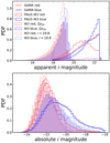 |
Fig. 4. Apparent (observed) and absolute i-band magnitudes of galaxies in PAUS (solid lines; limited to 0.1 < zphot < 0.8 and apparent i > 18) and GAMA (shading), with colours reflecting the (LEPHARE) red/blue selections displayed in Fig. 3 (top-left panel). We also display the magnitude distributions for 2 subsets of PAUS: (i) the best 50% selected on photo-z quality parameter Qz (dashed), and (ii) with apparent r < 19.8 (dotted) – approximately matching the GAMA flux-limit. Each histogram is individually normalised to unit area under the curve. Whilst the red galaxies in PAUS/GAMA are fairly similarly distributed in absolute i-band magnitude, PAUS exhibits a higher fraction of intrinsically faint blue galaxies. PAUS absolute magnitudes shown here are those computed using LEPHARE. |
2.4. Galaxy shape estimation
To measure the shapes of the galaxies we use weighted quadrupole moments2Iij which are defined as
 (2)
(2)
where f(x) is the observed i-band galaxy image (flux), W(x) is a suitable weight function to suppress the noise, I0 is the weighted monopole moment, and xi, xj denote the image coordinate axes. The moments are combined to form the ‘polarisation’, which quantifies the shape
 (3)
(3)
The resulting shapes are, however, biased; firstly, the weight function changes the quadrupole moments with respect to the unweighted case. Although this reduces the noise in the quadrupole moments, the estimate of the polarisation involves a ratio of moments that are noisy themselves. This leads to the so-called ‘noise bias’ (Kacprzak et al. 2012; Viola et al. 2014). Finally, the observed image f(x) is convolved with the point spread function (PSF).
A wide range of algorithms has been developed to relate the observations to unbiased estimates of the gravitational lensing shear. Our objective is very similar, although we note that an unbiased shear estimate is not quite the same as an unbiased ellipticity estimate. Here we use the algorithm developed by Kaiser et al. (1995) and Luppino & Kaiser (1997), with modifications described in Hoekstra et al. (1998), to correct the observed polarisations for both the weight function and the blurring by an (anisotropic) PSF. We refer the reader to these papers for further details.
The estimate for the ellipticity3 is given by
 (4)
(4)
where the smear polarisability Psm quantifies the response to the smearing by the PSF, and  captures the PSF properties. The pre-seeing shear polarisability Pγ corrects for the circularisation of the shapes by both the PSF and the weight function. Formally a 2 × 2 tensor, we assume it is diagonal with both elements having the same amplitude. Both polarisabilities involve higher order moments and
 (5)
(5)
is a combination of the shear polarisability Psh which captures the response to a shear for weighted moments, and the smear polarisability of both the galaxy and the PSF. As shown in Hoekstra et al. (1998), the PSF moments and polarisations should be measured using the same weight function as was used for the galaxies.
In principle, one is free to choose any weight function to estimate the galaxy ellipticity, but for intrinsic alignment studies this may affect the signal: a broader weight function is more sensitive to the outskirts of a galaxy compared to a more compact kernel. As tidal processes typically affect larger galactic radii, the IA signal may then depend on the choice of filter width. This was confirmed most convincingly by Georgiou et al. (2019a), but also see Singh & Mandelbaum (2016).
To allow for a comparison with the IA signals presented in Johnston et al. (2019), we choose the width of the weight function so that it resembles the one employed by Georgiou et al. (2019b). The weight function for the bright galaxies studied in these papers was based on an isophotal limit:  , where Aiso is the area above 3× the background noise level as determined by SEXTRACTOR (Bertin 1996). Although less susceptible to prominent bulges in well-resolved galaxies, this definition is difficult to link to the weight functions typically used in weak lensing studies. Moreover, the size depends upon the depth of the particular data set used, and thus is not uniquely defined.
In weak lensing studies, the width of the weight function matches the size of the observed galaxy image. Although this depends somewhat on the image quality, in practice it is better defined. As a compromise, however, we increase the width of the weight function to 1.75 times the observed half-light radius of the galaxy, as we found that this roughly matches the width used by Georgiou et al. (2019b).
2.5. Calibration of estimated ellipticities
Although Eq. (5) yields decent estimates for the ellipticities of the relatively bright galaxies considered here, these estimates are still biased. Moreover, the use of a wider weight function will increase the noise bias. To account for these biases, we follow Hoekstra et al. (2015) and create simulated images to determine the multiplicative bias correction as a function of observing conditions; that is to say, the seeing and galaxy properties dictating objects’ size and S/N.
The setup of the image simulations is similar to the one used in Hoekstra et al. (2015), and we refer the interested reader to that paper for greater detail. The galaxy properties are drawn from a catalogue of morphological parameters that were measured from resolved F606W images from the Galaxy Evolution from Morphology and SEDs survey (GEMS; Rix et al. 2004). These galaxies were modelled as single Sérsic models with galfit (Peng et al. 2002). We assume that the morphological parameters of the galaxies do not depend on the passband, although we note that our calibration should be able account for such differences. The background noise level is matched to the average value in the CFHTLS i-band data. The background varies in the data, but again, our calibration uses the S/N, which naturally accounts for the variation in noise level (see Hoekstra et al. 2015).
To measure the bias in the simulations we match the galaxies to the input catalogue and determine the best fit
 (6)
(6)
where μi is the multiplicative bias and ci the additive bias, which is found to be zero for our axisymmetric PSF. Moreover, we find that μ1 and μ2 agree with one another, so we only consider the average bias μ henceforth.
Similarly to Hoekstra et al. (2015), we assume that the multiplicative bias is predominantly determined by the angular size of the galaxy and the S/N. As a proxy for the size of the galaxy before convolution by the PSF, we define the parameter R as
 (7)
(7)
where rh, * denotes the half-light radius of the PSF and rh, obs that of the observed galaxy. However, to better capture the PSF dependence, we create images with seeing ranging from  to
to  and derive the correction as a function of seeing.
For a given PSF size, we determine μ in narrow bins of signal-to-noise ratio ν and galaxy size-proxy R. We found that the multiplicative bias μ can be parameterised fairly well by
 (8)
(8)
where the parameters αj are determined by fitting this model to the estimates of μ from Eq. (6).
As the IA measurements are limited to galaxies with i < 22.5, we calibrate the multiplicative bias for this range in magnitude. Figure 5 shows the values of the model parameters as functions of seeing. The resulting parameters minimise the bias for our sample, but we verified that the biases are also significantly reduced outside this magnitude range. Nonetheless, the residual bias does vary with magnitude, and the correction needs to be recomputed if different magnitude ranges are considered, because it changes the underlying population of galaxies (see Kannawadi et al. 2019).
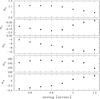 |
Fig. 5. Best fit parameters αj as a function of seeing. These parameters are used to estimate the multiplicative bias as a function of galaxy size and signal-to-noise ratio. |
Figure 6 shows the multiplicative bias μ as a function of seeing for simulated galaxies with 20 < i < 22.5, overlaid with the seeing distribution from the measured PSF sizes for each of the CFHTLS Megacam chips. The red points are the Kaiser et al. (1995; KSB) estimates, which show a clear dependence on seeing. Without an additional correction the mean bias ⟨μKSB⟩= − 0.051.
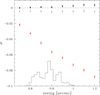 |
Fig. 6. Multiplicative bias μ as a function of seeing for simulated galaxies with 20 < i < 22.5. The red points correspond to the KSB estimates, which are significantly biased and depend upon image quality. The corrected biases are shown as grey (per-galaxy bias correction) and black (seeing-averaged bias correction) points. The histogram shows the seeing distribution for the CFHTLS W3 data. |
Equation (8) and the resulting fitted parameters in Fig. 5 describe a model to estimate the required multiplicative ellipticity bias correction, as a function of a given object’s size R and signal-to-noise ratio ν. One approach to calibration is to use the model to apply corrections to each simulated galaxy individually; we do this and show the residual bias (grey points) in Fig. 6. The mean residual bias for this approach is ⟨μcor⟩= − 0.0045. Alternatively, we can average the model estimates of the bias within bins of seeing, and apply these averaged corrections to the galaxies falling in each bin, thus lessening the impact of noise from individual galaxy shapes. These corrections are shown in Fig. 6 as black points, with a mean of ⟨μcor⟩ = 0.0012 – slightly better than the first approach, and sufficient for our IA work here.
As we aim to measure the IA signal for samples split by morphology (which roughly correlates with our colour-split) it is worth examining whether our correction can be used in this case. We measured residual bias when we split the sample at input Sérsic-index nin = 2, chosen for indicative purposes (see e.g., Vakili et al. 2020, Fig. 2). For galaxies with nin ≤ 2 we find ⟨μcor⟩ = 0.0048 and for nin > 2 we obtain ⟨μcor⟩= − 0.0114; although the bias depends on the radial surface brightness profile, the differences are too small to affect our results. In any case, we calibrate our PAUS red and blue sample ellipticities according to the seeing-averaged multiplicative biases calculated within each colour-split sample.
2.6. Photo-z quality
We investigate the quality of the photo-z estimates in W3, plotting the Qz parameter4 and zphot. against zspec. for ∼4k PAUS galaxies matched to the spectroscopic DEEP2 (Newman et al. 2013) DR4 catalogue in Fig. 7. We see that the quality of zphot. drops with increasing zspec. (small Qz = good zphot.), and that there is no drastic performance differential between red and blue galaxies. Figure 8 looks deeper, considering the redshift error zphot. − zspec., normalised by 1 + zspec., as a function of the LEPHARE rest-frame colour u − i. The 16th, 84th percentiles are shown for each colour as dashed lines, and as solid lines for the best 50% of photo-z according to the Qz parameter. For the Qz-selection, half the difference between the percentiles is quoted for each colour as σ68, with the full-sample σ68 given in brackets. We see that red galaxies have marginally lower quality zphot. than blue galaxies when selecting on Qz, and that this behaviour is reversed over the full sample, with red photo-z performing better. We also see that all zphot. have a tendency to be under-estimated with respect to the spectroscopic redshifts.
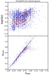 |
Fig. 7. Top: photo-z quality log(Qz) for ∼4k PAUS-DEEP2 matched galaxies, as a function of their spectroscopically determined redshifts zspec., with red and blue colours reflecting the LEPHARE classification of the galaxies (see Fig. 3, top-left panel). A smaller value of Qz indicates a higher-quality photo-z estimate. Bottom: PAUS photo-z estimates vs. DEEP2 spec-z, again coloured by galaxy classification. The 1-to-1 relation is shown in the bottom panel as a faint yellow dashed line. |
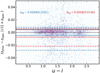 |
Fig. 8. Hexagonally-binned 2D histogram of PAUS-DEEP2 matched galaxies’ photo-z error, normalised by their spectroscopic redshifts and as a function of their LEPHARE rest-frame colour u − i. Shading indicates the log-counts in each cell. For the best 50% of photo-z according to the Qz parameter, we display the 16th, 84th percentiles of the normalised photo-z error for red (blue) galaxies as solid red (blue) horizontal lines. Half the difference between the percentiles is quoted for each as σ68. Dashed lines and bracketed values of σ68 are then for the total sample. |
Considering the sparsity of PAUS W3 objects beyond zphot. ∼ 0.8 (Fig. 3), and the small volume probed (by just ∼19 deg2) at zphot. ≲ 0.1, we restrict our measurements to PAUS galaxies in the range 0.1 < zphot. < 0.8. We note that Fig. 7 suggests a drop in the quality of photo-z at zphot. ∼ 0.7 – we discuss the potential for mitigation of photo-z errors with random galaxy catalogues in Sect. 3.3.
2.7. GAMA
The Galaxy and Mass Assembly (GAMA; Driver et al. 2009, 2011; Baldry et al. 2018) survey was conducted at the Anglo-Australian Telescope, and the final data were described by Liske et al. (2015). GAMA achieved high completeness (≳98%) down to r < 19.8 over 180 deg2 within the equatorial fields G9, G12, G15 (60 deg2 apiece). We compare the correlation functions we measure in PAUS with analogous measurements made in GAMA and presented in Johnston et al. (2019), where details of shape measurements (from Kilo Degree Survey imaging: de Jong et al. 2013; Georgiou et al. 2019a), sample characteristics, covariance estimation etc., can be found. The observed and absolute magnitude distributions of galaxies in GAMA are compared with those from PAUS, for red and blue galaxies, in Fig. 4.
We list some summary characteristics for our PAUS W3 and GAMA samples in Table 1, including sample counts, mean redshifts and mean luminosities, relative to a pivot luminosity Lpiv. corresponding to absolute Mr = −22 – this is for comparison with literature studies of IA (e.g., Joachimi et al. 2011; Johnston et al. 2019; Fortuna et al. 2021).
PAUS W3 (0.1 < zphot. < 0.8) and GAMA sample characteristics.
3. Random galaxy catalogues
Configuration-space statistics involving galaxy positions typically rely upon sets of random points as Monte Carlo samples of the observed survey volume. Galaxy densities are taken in ratio to the density of these un-clustered points, which grant a notion of the local ‘mean’ density. In addition, the subtraction of statistics measured around random points, from those measured around galaxies, helps to mitigate biases coming from survey edge effects and spatially correlated systematic effects in studies of, e.g., intrinsic alignments and galaxy-galaxy lensing (Singh et al. 2017).
Our objective here is to explore the clustering and IA of PAUS galaxies over short separations in three dimensions, thus our randoms need to reproduce both the radial and angular selection functions of the data, without structure and at high resolution. The latter selection function is trivially reproduced, as we are able to construct an angular mask from observed galaxy positions, within which we can assign uniformly distributed on-sky positions to random points – thus replicating the survey window and stellar masking from Fig. 1.
The radial selection function is more difficult to characterise, as simple fits to, or reshuffling of, the galaxies’ n(z) would retain structural information and act to erase line-of-sight correlations. Moreover, we intend to make sample selections in the galaxy data to capture the galaxy type-dependence (and, in future work, any redshift-evolution, luminosity dependence etc.) of IA/clustering phenomena – these selections will change the galaxies’ n(z) and must be reflected in the radial distribution of randoms. To tackle these challenges, we chose to follow and adapt the galaxy-cloning method introduced by Cole (2011) and employed in the GAMA survey clustering analysis of Farrow et al. (2015).
3.1. Vmax randoms
The method uses indirect estimates of the galaxy luminosity function (LF) to predict an un-clustered n(z). Given the survey limiting characteristics and galaxy properties, one can compute for each galaxy the maximum volume Vmax within which it could be observed – this corresponds directly to a maximum redshift zmax, dependent upon the survey flux-limit and galaxies’ k + e-corrected magnitudes in the relevant detection band. k-corrections modify magnitudes to account for redshifting of SEDs, whilst e-corrections account for their evolution; to estimate the magnitude of an object were it at z = 0, one must consider that the object’s SED would be more evolved in this case, hence the observed magnitudes need an additional correction. We computed zmax via the relations
 (9)
(9)
where Mz = 0 denotes the rest-frame absolute magnitude at z = 0, m are observed/limiting apparent magnitudes, μ are the observed/maximum distance moduli5, k0(z) are k-corrections from redshift z to zero, and Q(z − zref)≡e(z) parameterises the evolution correction between a galaxy redshift z and a reference redshift zref – assuming galaxy magnitudes to evolve linearly with redshift. This parameterisation is highly approximate, and will not correctly capture the complex evolution of stellar populations over cosmic time; a more comprehensive treatment could make use of spectral synthesis models, though that is beyond the scope of this work.
The maximum volume is
 (10)
(10)
where we have not yet included the effects of redshift evolution (see Cole 2011). zmin allows for a possible bright cut-off, beyond which highly luminous galaxies are discarded. A standard estimator (Eales 1993) for the LF is
 (11)
(11)
that is to say, the inverse-Vmax weighted sum over galaxies with luminosity L – we can thus use our computed Vmax per galaxy to create a randoms catalogue, without radial structure and with a consistent LF, simply by cloning each real galaxy many (Nclone) times and scattering them uniformly within their respective Vmax.
However, this estimator is vulnerable to bias; galaxy surveys are subject to sampling variance, and thus exhibit significant over/underdensities in the radial dimension – these will translate into over-/under-representation of luminosity populations. An equal number of clones per galaxy would then over-fit the galaxy n(z), and suppress any measured galaxy clustering. Cole (2011) introduced a maximum likelihood estimator for the LF, computed with a density-corrected Vmax, dc which acts to down-weight the contribution of galaxies in overdense environments, e.g., clusters. Vmax, dc is computed as
 (12)
(12)
where Δ(z) is the fractional overdensity as a function of redshift. Vmax, dc can be substituted into Eq. (11) to yield a more robust estimate of the luminosity function. Following Cole (2011) and Farrow et al. (2015), we use the individual ratios of Vmax to Vmax, dc to re-scale the number of clones per galaxy n = NcloneVmax/Vmax, dc, such that they are over-produced in underdense environments, and vice-versa.
Δ(z) is estimated through an iterative process, starting with Δ(z)≡1 (i.e. Vmax ≡ Vmax, dc). We scatter Nclone clones per galaxy, uniformly throughout their respective Vmax, and estimate Δ(z) as
 (13)
(13)
One then re-computes Vmax, dc, re-weights the number of clones, re-generates the randoms’ n(z), and repeats the process until Δ(z) converges – we allowed for 15 iterations, though convergence was typically reached after ≲10. Creating randoms for Q ∈ [ − 1.5, 1.5], with a spacing of 0.1, we found on inspection of the PAUS W3 n(zphot.) that the Q = 0.2 randoms provide the best match to the redshift distribution – we leave a more detailed optimisation of Q, or a more complex treatment of e-corrections, to future work.
3.2. Windowing
Thus far, we have ignored the redshift evolution of the luminosity function. Cole (2011) outlines methodology to include a parameterised model for the evolution, to be constrained by the data. To avoid the need for some parametric LF-evolution model, we implement the ‘windowing’ alternative employed by Farrow et al. (2015), wherein each galaxy’s Vmax is limited by a window function centred on its observed radial position. Galaxy clones are then scattered only within the window, limiting their presence in disparate redshift regimes and thus building the z-evolution into the randoms.
Each window takes a Gaussian form, truncated at ±2σ such that ∼71.5% of a galaxy’s clones will exist within a 1σvolume deviation from its observed redshift – this means that the window is elongated towards the observer in the radial dimension, as the observed volume diminishes due to the light-cone effect. It is necessary that each window be reflected at any boundaries – i.e. z = 0, zmin, zmax or the limits of the survey – in order to prevent an excessive stacking-up of clones in the centre of the randoms’ redshift distribution.
The choice of width σ for the Gaussian is fairly arbitrary, however it clearly must be large enough that radial large-scale structure is not over-fitted, and small enough to achieve the desired preservation of luminosity populations over redshifts in the clones. We produce windowed randoms for PAUS with σ = 6 × 10⁶ (h−1 Mpc)3, chosen to satisfy these requirements. The window function, recast as a function of redshift/comoving distance, is included in the integrals of Vmax and Vmax, dc (Eqs. (10) and (12)) so that clone-counts are correctly adjusted for the new, Gaussian-weighted volumes.
Figure 9 shows the PAUS 40-NB photometric redshift distribution, with the spectroscopic redshifts of available DEEP2 galaxies, and overlaid with redshift distributions for our un/windowed, cloned randoms. The bottom panel gives the overdensity Δ(z) as a function of redshift. To illustrate the utility of galaxy cloning, Fig. 10 also shows the photo-z distributions of (LEPHARE) red and blue galaxies in PAUS W3 (see Fig. 3), along with those of their relevant random clones. One sees that the general trends levied by the selection are reproduced by both un/windowed randoms, though the windowing restriction causes differences, especially for the red galaxy randoms.
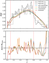 |
Fig. 9. Top: photometric redshift distribution of PAUS W3 (black solid), with spectroscopic redshifts of the DEEP2-matched galaxies (grey dashed), overlain with the randoms’ n(z), generated with and without the windowing (Sect. 3.2) and photo-z (‘zph-randoms’; Sect. 3.3) approaches, as indicated in the legend. Bottom: density contrast Δ(z) (Eq. (13)) computed after the final iteration of clone dispersal for each set of randoms – for zph-randoms, the ratio ngal(z) / nrand.(z) (Eq. (13)) is computed against galaxy redshifts drawn from n(zspec. | zphot.) (see Sect. 3.3), such that ngal(z)≠n(zphot.) and Δ(z) / Nclone can be greater than unity where nrand.(z) > n(zphot.), e.g., at zphot. ∼ 1. Our zph-randoms methods yield smoother redshift distributions, more faithful to the available n(zspec.). Red vertical lines delimit the redshift range employed in our correlation function analysis. |
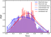 |
Fig. 10. Photometric redshift distributions of PAUS W3 galaxies, split into (LEPHARE) red/blue samples (shaded histograms), along with the n(z) for red/blue clones in the windowed randoms (solid lines) and the unwindowed randoms (dashed lines). Randoms shown here are the ‘zph-randoms’ described in Sect. 3.3. Each histogram/curve is individually normalised to unit area. |
The effects of windowing are illustrated in Fig. 11, which closely mimics Fig. 3 from Farrow et al. (2015). The top-panel shows the unwindowed random clones’ redshift distributions for photo-z selections in PAUS W3, while the bottom-panel shows the same for σ = 3 × 10⁶ [h−1 Mpc]3 windowed clones – we show a smaller window-size in Fig. 11 for emphasis of the windowing effect. One clearly sees the restriction of clones to redshifts near their parent galaxy. The numerous clones at very low redshifts (red curves plateau towards z = 0) correspond to faint, near-universe galaxies with small values of zmax – these are excluded from our analysis in any case.
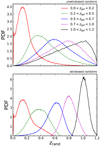 |
Fig. 11. Redshift distributions of random clones zrand, whose parent galaxies are situated at photometric redshifts zgal. Top: unwindowed clones are scattered over the entire redshift range, depending on the brightness, and hence zmax, of parent galaxies. Bottom: for the windowed randoms, 71.5% of a galaxy’s random clones are scattered within a ±1σ symmetric volume, centred on the location of the parent galaxy [we display σ = 3 × 10⁶ (h−1 Mpc)3 randoms here, for a clearer illustration]. We note that the symmetry is in volume coordinates, hence in redshift/comoving coordinates the windows are extended in the direction of the observer, and slightly squashed in the outward direction. This figure is closely based on a similar plot presented by Farrow et al. (2015) for GAMA galaxies and randoms (their Fig. 3). Plateaus in the red curves, on approach to redshift zero, correspond to faint, very low-redshift galaxies which are excluded from our analysis. |
3.3. Photo-z impact and ‘zph-randoms’
As previously mentioned, Fig. 7 reveals a dip in photo-z accuracy whereby many PAUS-DEEP2 galaxies at zspec. ≳ 0.7 are assigned zphot. ∼ 0.7 by the BCNZ2 algorithm – this is currently under investigation. In the meantime, we note the consequences in Figs. 9 and 10, where each set of randoms seemingly overpopulates redshifts z ≳ 0.8, relative to the PAUS W3 n(zphot.). This is because (i) the number of PAUS galaxies beyond zphot. ∼ 0.8 should be higher (Fig. 7), and (ii) the inferred zmax are biased for many galaxies with zphot. ∼ 0.7, due to significant errors in zphot. (i.e. in the observed redshift zobs. in Eq. (9) – these biases are also responsible for the low-redshift ‘bumps’ exhibited by randoms in Fig. 9, where galaxies’ zmax have been underestimated). Consequently, the randoms ‘see’ a large underdensity at z > 0.8 and respond by over-filling the volume with clones. The windowed randoms restrict the clones to redshifts near to their parent zphot., resulting in the marginally tighter fit to the data in Fig. 10.
Using GAMA as a test-bed, we investigated the photo-z degradation of measurable signals, and the consequences of generating randoms using photo-z. In order to roughly mimic the pathologies present in the PAUS photo-z distribution, we applied a Gaussian6 scatter σzphot. to GAMA spec-z according to
 (14)
(14)
where i is the observed i-band magnitude of a galaxy, and i50 is the 50th percentile of all i-magnitudes in the range 14 < i < 20.5 – thus fainter objects suffer larger scatters. We further applied a probabilistic ‘kick’ to GAMA spec-z in order to mimic photo-z outliers. The probability Pkick of a galaxy receiving a kick is implemented as
![Mathematical equation: $$ \begin{aligned} P_{\rm kick} = 0.15 \, \frac{i}{i_{50}} + \mathcal{N} [0,\,0.003], \end{aligned} $$](/articles/aa/full_html/2021/02/aa39682-20/aa39682-20-eq19.gif) (15)
(15)
where the Gaussian draw introduces stochasticity about the relation, and the kick δz itself is uniformly drawn from 0.07 < δz < 0.08 before a random 60% are given a negative sign – such that model catastrophic photo-z failures tend to underestimate the true redshifts (Fig. 8). σzphot. and Pkick are illustrated in the bottom-panels of Fig. 12, as functions of the i-band magnitude, and coloured by the GAMA spectroscopic redshifts of objects. Finally, to model the stacking-up of photo-z estimates at zphot. ∼ 0.7 in PAUS, we re-located to zphot. = 0.27 + 𝒩[0, 0.025] (a) a random 3% of all GAMA spec-z, and (b) a number of galaxies around zspec. ∼ 0.35, with the probability of relocation equal to 40% at the zspec. = 0.35 peak, and decaying as a Gaussian (σ = 0.025) to either side.
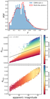 |
Fig. 12. GAMA spectroscopic redshift distribution (top-panel; blue), overlaid with our approximately PAUS-like photometric redshift distribution (top-panel; red) – these photo-z are created by applying a redshift- and magnitude-dependent Gaussian scatter (middle-panel; Eq. (14)) to the spec-z, along with a probabilistic ‘kick’ (bottom-panel; Eq. (15)) to generate catastrophic outliers, and a manual relocation of some galaxies to zphot. ∼ 0.27 (see Sect. 3.3). Bottom-panels are hexagonally-binned 2D histograms, with cells coloured according to the mean GAMA spec-z of objects residing in each cell. |
The resulting redshift distribution (Fig. 12, top-panel) is thus smoothed, as is typical for photo-z distributions, and features a peak at zphot. ∼ 0.27 followed by a sharp drop – these redshifts provide our PAUS-like7 photo-z testing ground for a new method of redshift-assignment for random points: employing galaxy redshifts sampled from conditional distributions n(zspec. | zphot.), rather than photo-z estimates themselves. The aforementioned biases in zmax estimates, due to the inaccuracies inherent to photo-z, can be mitigated over the galaxy ensemble if we draw many realisations of a ‘spectroscopic’ n(z) from the probability density distributions n(zspec. | zphot.) surrounding each galaxy’s zphot. – after testing, we settled upon 320 draws per object, from n(zspec. | zphot. ± 0.03) for GAMA, and we increased this to 500 draws from the conditional range zphot. ± 0.04 for PAUS. The resulting distributions of zmax are illustrated in Fig. A.1 for a random selection of GAMA galaxies.
Repeating our randoms-generation procedure from Sects. 3.1 and 3.2 for each of the 320 realisations of GAMA, we created ensemble-sets of randoms which encode the characteristic errors in the photo-z distribution, as traced by the available spec-z8. We illustrate the outcomes of this procedure in Figs. 13 and 14, which display the n(zspec.) vs. n(zphot.) plane for galaxies/randoms, and some ‘marginals’ through the plane, respectively. One sees from the contour-plot (Fig. 13) that the deviations from 1-to-1 correspondence in the data are smoothly traced by the randoms, and this is made clearer in Fig. 14, where the hand-made peak at zphot. ∼ 0.27 (solid line) is captured by our ensemble [σ = 5 × 10⁶ (h−1 Mpc)3] windowed randoms (dashed line) in the final panel.
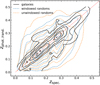 |
Fig. 13. Contours depicting cumulative population fractions 0.08, 0.25, 0.42, 0.58, 0.75 and 0.92 for GAMA galaxy/zph-randoms catalogues on the zphot./rand. vs. zspec. plane, where the y-axis refers to zphot. for galaxies and zrand. for randoms. For randoms, zspec. refers to the spectroscopic redshift of the parent galaxy to a clone at redshift zrand.. Blue contours depict our windowed randoms, with window-width σ = 5 × 10⁶ (h−1 Mpc)3, and orange contours are for unwindowed randoms. One clearly sees the intentional photo-z biases (Sect. 3.3) in the galaxy contours (solid black), and how the randoms (dashed colours) softly mimic them. Figure 14 shows five ‘marginals’ through this distribution for (zph-windowed randoms only), collapsing the y-axis to show n(zspec. | zphot.). |
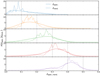 |
Fig. 14. Spectroscopic redshift distributions of GAMA galaxies, binned by the mock photometric redshifts we describe in Sect. 3.3. Vertical black lines depict the bin-edges in zphot. and solid curves give the resulting n(zspec. | zphot.) for galaxies. Selecting only the clones of those binned galaxies, from our ‘zph-windowed’ GAMA randoms [σ = 5 × 10⁶ (h−1 Mpc)3], the randoms’ redshift distributions are then given by the dashed curves. One sees that our ‘zph-randoms’ [generated using samples from the n(zspec. | zphot.)’s centred on individual galaxies’ zphot. – see Sect. 3.3] are thus able to trace the artificial photo-z biases – for example, the secondary peak at z ∼ 0.3 in the final panel, which is captured by the tail of the randoms’ n(z). These curves are equivalent to horizontal bands in Fig. 13, summed over the y-axis. |
To assess the performance of these ‘zph-randoms’, we compare intrinsic alignment and clustering correlations in GAMA, measured using spec-/photo-z and various random galaxy catalogues, presenting results in Appendix A. In particular, we see that this ‘excess’ of randoms at z ∼ 0.27, matching the photo-z-induced galaxy excess there, is important; correlated galaxy pairs at these redshifts have some real range of transverse separations rp, but are included in 3D correlation function estimators at separations > rp because they are thought to be at higher redshifts due to photo-z errors. This causes a tilting of observed correlations (see Fig. A.2), as small-scale power is erroneously pushed to larger scales – the excess in the randoms, however, mitigates this effect by suppressing long-range correlations. Next, we detail our methodology for measuring projected correlations.
4. Two-point statistics
With random galaxies uniformly permeating the survey volume, we are now free to measure the galaxy clustering and alignments with a radial binning of galaxy pairs. Since PAUS is a unique survey, we lack samples against which to directly compare galaxy statistics.
Photometric redshift scatter acts as a radial smoothing of the 3D galaxy density field, suppressing the observable clustering as galaxy pairs which are not in fact correlated pollute the desired signal. Thus we expect any clustering signal from PAUS to be lower in amplitude than the equivalent signal from a spectroscopically observed sample. One expects a similar dilution for the intrinsic alignment signal, as uncorrelated galaxy pairs are mistakenly included in the estimator.
As such, we choose to compare our PAUS signals with those measured in GAMA using our PAUS-like mock photo-z. We stress that this procedure is highly approximate, and intended only to be instructive – photo-z scatter is often a function of galaxy properties, which are in turn correlated with environments. Thus our degradation of GAMA redshifts, whilst reminiscent of PAUS over the full n(z), may not match the severity or complexity of the degradation already present in PAUS. PAUS is also deeper than GAMA, and has less area; the signal-to-noise will peak in a different regime. For these reasons, the signal-comparison ought not to be considered rigorous.
4.1. Clustering
The Landy-Szalay (Landy & Szalay 1993) estimator for the galaxy correlation function is
 (16)
(16)
where the various galaxy-galaxy (DD), random-random (RR) and galaxy-random (DR) pair-counts are binned by transverse rp and radial Π comoving separations. Subscripts i, j label the galaxy (D) samples and their corresponding randoms (R); i = j for a sample auto-correlation. In this work, we display only the galaxy clustering auto-correlations; blue-blue and red-red sample clustering. This is done to provide a direct comparison between the clustering of red and blue galaxies, though future analyses will make use of full-sample clustering correlations in order to constrain the galaxy bias in tandem with IA correlations. Here, we have used the full (unselected) PAUS W3 sample as a positional tracer for IA correlations, thus improving the signal-to-noise and eliminating the effects of differential galaxy bias in the ‘density’ samples (see Eq. (19)).
The projected clustering correlation function is then
 (17)
(17)
Working with a log-spaced binning in rp of 5 bins between 0.1 and 18 h−1 Mpc, we explored different choices of binning in Π to accommodate the effects of photo-z scatter. The standard approach, utilised for spectroscopic data, is to perform a Riemann sum over uniform bins in Π, e.g., with dΠ = 4 h−1 Mpc and |Πmax| = 60 h−1 Mpc (as in e.g., Mandelbaum et al. 2006a, 2011; Johnston et al. 2019). With precise redshift information, these limits capture the vast majority of correlated galaxy pairs without introducing excessive noise due to the inclusion of uncorrelated objects. In the photometric case, however, the signal is smeared-out along the Π-axis, and correlated pairs are lost from the estimator. We explored a ‘dynamic’ binning in Π, where bins increase in size from small to large values of Π – thus physically associated objects are brought back into the estimator, and the impacts of integrating over noise at large-Π are mitigated with broader bins. We implemented this binning as an adapted Fibonacci sequence9, up to a |Πmax| of 233 h−1 Mpc, such that the bin-edges are
 (18)
(18)
We shall display signals measured with both the standard, ‘uniform’ and new, dynamic binning in Π. With this Π-binning, and our ‘zph-randoms’ (Sect. 3.3), we hope to recover as much lost signal as possible, whilst simultaneously mitigating the impacts of photo-z outliers upon the signals, thus simplifying the modelling of correlations in future work.
4.2. Alignments
With the same rp, Π binning choices, we also measured the projected galaxy position-intrinsic shear correlations wg+ for our PAUS galaxy samples, using the estimator (Mandelbaum et al. 2006a)
 (19)
(19)
for which
 (20)
(20)
D here denotes the ‘density’ sample of galaxies, which forms the ‘position’ component of the correlation (as mentioned above, this is the full, all-colour galaxy sample for PAUS), S+ denotes the ‘shapes’ galaxy sample and S+X is the sum of ellipticity components of galaxies i from the shapes sample, relative to the vectors connecting them to galaxies j from sample X, normalised by the shear responsivity10  , where σϵ is the S sample shape dispersion. The shape- and density-sample randoms are denoted RS and RD, respectively, and RSRD are the normalised pair-counts between the different randoms. We note that the standard convention for wg+ is that positive signals indicate radially aligned galaxies11.
Rotating ellipticities by 45°, ϵ+ → ϵ× in Eq. (20), and we measure the position-shape cross-component  – a non-vanishing cross-component would indicate some preferred direction of curl in the galaxy shape distribution, breaking parity and thus signalling the presence of systematics in shape estimation.
  and
and  are constructed from
  and
and  in exact analogy to Eq. (17). We present the significance of measured wg× correlations in Appendix A.
We note that increasing the maximum permissible line-of-sight separations Πmax (Eq. (18)) for galaxy pairs risks the contamination of our intrinsic alignment statistics wg+, wg× by genuine galaxy-galaxy lensing (GGL) signals – that is, correlations between foreground galaxy positions and background gravitational shears. The amplitude of any such contribution depends upon the width of the true (i.e. not photometric) distribution of Π across all pairs considered. With |Πmax| = 233 h−1 Mpc, any GGL contribution should be strongest from lenses at ∼233 h−1 Mpc paired with sources at about twice the lens distance, and dropping off at higher redshifts where efficiently lensed sources are excluded by Πmax. Photo-z errors could spuriously promote more distant sources into the estimator (Eq. (19)), and any coherent tangential shears around the foreground density field would then be negative in the ξg+ correlation – given the quality of PAUS photo-z, and given that we limit our analysis to zphot. > 0.1 (≳420 h−1 Mpc), we expect any GGL contribution here to be weak; future work with more area and greater signal-to-noise can test for contamination of IA correlations by enforcing large line-of-sight separations in Eq. (19) (i.e. setting some |Πmin|), and should consider this possibility when attempting intrinsic alignment model-fitting.
4.3. Covariance estimation
We estimated errors for the correlations via a delete-one jackknife resampling of the observed volume. Splitting the PAUS W3 footprint into eight roughly equal-area patches, we then defined redshift slices with comparable galaxy counts to create pseudo-independent jackknife sub-volumes. We defined three equally-populated slices of depth ≥466 h−1 Mpc, in order to accommodate the largest allowed line-of-sight separations in the case of our dynamic binning in Π, resulting in a total of 24 sub-volumes. The covariance is constructed for each correlation function w as
 (21)
(21)
where wα is the signal measured upon removal of jackknife sub-volume α, and  is the average of all jackknife signals wα. This definition of jackknife sub-volumes with variable redshifts implicitly assumes that any redshift evolution of the signal is small. Given the small area of PAUS W3, we are otherwise unable to define enough jackknife samples to minimise noise in the covariance, without the errors becoming severely inaccurate on the larger scales of interest – just 24 sub-volumes for 5 data-points is sub-optimal, though errors should then be reliable up to ∼19 h−1 Mpc for redshifts 0.1 < z < 0.8, thus encapsulating our range of considered scales for PAUS. Since the noise will be prominent in the off-diagonals of the covariance, and since we do not intend to perform any detailed line-fitting here, we proceed with the 3D jackknife, noting that a significant redshift-evolution of signals would result in our over-estimating the full-sample variance. We do make use of the full covariances in estimating the significance of detection for IA signals, and in fitting simple power-laws to clustering signals, to aid with comparison of different (with respect to colours, Π-binning, randoms and photo-z quality-cuts) correlation configurations – see Appendix A.
Any spectroscopic GAMA measurements shown are those presented in Johnston et al. (2019), with jackknife errors estimated from 45 sub-volumes of depth ≥150 h−1 Mpc, and with colour-selections applied to both density and shapes samples for IA correlations. We estimated errors for our mock photo-z GAMA samples with 36 sub-volumes of depth ≥260 h−1 Mpc, noting that the dynamic Π-binning scenario will consequently suffer slightly under-estimated errors, as pairs falling in the final Π-bin (Eq. (18)) are imperfectly captured. These signals are meant only to be instructive, hence we proceed as such.
5. Results
Projected correlation functions wg+, describing the radial alignment of galaxy shapes with galaxy positions, and wgg, the galaxy position auto-correlation, are displayed for PAUS W3 and GAMA in Fig. 15. For reasons detailed in Appendix A (where we also present successful systematics-tests wg×), we elected to compare with GAMA the PAUS signals measured using our LEPHARE colour-split (Fig. 3), our zph-windowed randoms (Sect. 3.3), and the dynamic binning in line-of-sight separation Π (Sect. 4.1) – the best-performing setup for our tests against the mock photo-z GAMA sample (Sect. 3.3 and Appendix A). The figure displays signals measured in PAUS W3 (solid pentagons/curves), for galaxies in the photo-z range 0.1 < zphot. < 0.8, along with spectroscopic signals from GAMA (open circles) and the signals measured in our mock photo-z GAMA sample (downward triangles) using the same randoms/Π-binning setup for treatment of photo-z errors. Grey-hatching indicates the regime where we would be unable to compute reliable errorbars for PAUS (see Sect. 4.3).
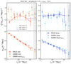 |
Fig. 15. Projected position-shear (top) and position-position (bottom) correlations measured for red (left) and blue (right) galaxies in PAUS (filled pentagons) and GAMA (open circles and filled triangles). The PAUS correlations displayed here are for all galaxies (i.e. not selected according to Qz), split by colour according to LEPHARE, measured with zph-windowed randoms and dynamic Π-bins – see Appendix A for details on our choice here. Downward triangles display the correlations measured in GAMA using our mock photo-z, described in Sect. 3.3. Grey hatching indicates the larger scales where our PAUS W3 jackknife would yield unreliable errorbars (see Sect. 4.3). |
Even with our treatment, one sees the degradation of strongly significant red galaxy IA signals from spectroscopic GAMA data when measured using our mock photometric redshifts; we can expect the real, inaccessible PAUS IA signature to be similarly degraded by photo-z scatter. Still, we are able to make a detection at ∼3.1σ for red galaxy alignments in PAUS W3, and the significance of signals is consistently much higher than for blue galaxies (see Appendix A).
Given the results in the literature (Mandelbaum et al. 2006b; Hirata et al. 2007; Joachimi et al. 2011; Johnston et al. 2019; Georgiou et al. 2019b), one might expect to find even more significant radial alignments in this sample. Joachimi et al. (2011) found such correlations in photometric red galaxy samples of similar intrinsic brightness, over similar redshift ranges. Their samples, however, spanned a much larger area on-sky (more than 150×) with respect to PAUS W3, consequently yielding smaller statistical errors, and being comparatively dominated by bright central galaxies; Johnston et al. (2019) found central galaxy shapes to be the highest S/N contributor to alignment signals. However, they also found that satellite galaxies – which will be more prevalent in PAUS – do play a role in sourcing wg+ signals via their positions, particularly on smaller scales; we think it likely that such a small-scale signal may be found in PAUS with more area and continued development of photo-z and their treatment.
To guide the eye, we computed some non-linear alignment model (NLA; Hirata & Seljak 2004; Hirata et al. 2007; Bridle & King 2007) predictions for wg+ using the PAUS-DEEP2 galaxies’ spectroscopic n(z), displaying these in Fig. 15 as green/blue dashed lines (top-left panel) – these curves are proportional to the product of a density sample galaxy bias bg and an intrinsic alignment amplitude AIA. We find that the difference in NLA model predictions computed for n(z) given by DEEP2 spec-z, or by BCNZ2 photo-z, is negligible. For reference, the AIAbg = 6 curve (green dashed) roughly corresponds to the constraints of Johnston et al. (2019), obtained by fitting jointly to red-red galaxy clustering and red-red position-intrinsic shear correlations measured in GAMA data, with shapes from Kilo Degree Survey imaging (KiDS; Kuijken et al. 2019).
More interesting for the PAUS sample are the blue galaxy alignments, which are consistent with zero (for both surveys), at high precision. This result is especially interesting given the differences in redshift and luminosity distributions of blue galaxies in PAUS and GAMA (Figs. 3 and 4); we have yet more evidence for a lack of intrinsically aligned blue galaxies, on scales of 0.1 − 18 h−1 Mpc, regardless of their selection (Hirata et al. 2007; Mandelbaum et al. 2011; Johnston et al. 2019). Despite the small area of PAUS W3 (∼19 deg2), the precision of blue galaxy signals is comparable with that from GAMA (∼180 deg2), even after adding noise via our dynamic Π-binning, owing to the increased depth and consequently high number density of PAUS. It should be considered that the aforementioned photo-z degradation of signals also applies here; however, the mock GAMA signals are noisier and less precisely null than the spectroscopic signals. Thus we might argue that the underlying signal for PAUS should be consistent with zero at high precision for the added noise to have so little effect. Indeed, every configuration we explore for the measurement of this blue galaxy IA signature yields signals that are non-zero at ≲0.8σ, typically not exceeding ∼0.4σ.
One might expect lower amplitudes of clustering in PAUS (compared with GAMA) for two reasons; (i) fainter galaxies are known to be less biased than brighter ones, and (ii) the photo-z scatter will create a general suppression of power, particularly on smaller scales. Therefore, taken at face-value, the PAUS blue galaxy clustering signal in Fig. 15 is of surprisingly high amplitude with respect to spectroscopic GAMA; blue galaxies in PAUS are on average much fainter than those in GAMA (Fig. 4), and subject to photo-z errors which are expected to lower amplitudes and perhaps flatten power laws (by more efficiently suppressing small-scale signals). Complicating matters further, these data-points are highly correlated, making by-eye comparisons less instructive. We summarise our clustering results for each different correlation configuration in Appendix A, and state here our general findings: blue galaxy clustering in PAUS is seen to exhibit a shallower gradient from small to large scales, with respect to GAMA, and to have typically smaller or comparable amplitudes at rp = 1 h−1 Mpc, except when using dynamic Π-bins and selecting on photo-z quality via Qz (see Fig. A.4) – the use of either dynamic bins or photo-z selection alone yields similar amplitudes/slopes, with little sensitivity to the choice of randoms.
As Fig. 4 shows, red galaxies in PAUS are of roughly similar intrinsic brightness to those in GAMA, making the high amplitude of that signal less concerning. We see a steeper power law with respect to GAMA, going against the prediction for photo-z degradation – curiously, we see similarly steep correlations for the mock GAMA sample, perhaps signalling a differential impact of our mock photo-z errors coming from magnitude-colour correlations inherent to any galaxy sample; redder galaxies tend to be brighter, such that Eqs. (14) and (15) will behave differently for red and blue objects. However, the aforementioned concerns with respect to correlations between rp-scales also apply here, thus we neglect to investigate further, noting that a more realistic mock photo-z implementation will aid with disentangling these results. We generally find greater consistency with spectroscopic GAMA clustering for red galaxies, with only slightly steeper gradients and slightly lower amplitudes – see Appendix A for a more complete breakdown of signals from our various correlation configurations.
In future work, we will repeat and improve upon this analysis with the full PAUS area; the statistical power offered by PAUS will then be competitive with GAMA, providing new avenues and physical scales for directly constraining intrinsic alignment models – such as the IA halo model with specific prescriptions for red and blue, central and satellite fractions, as they evolve with redshift (Fortuna et al. 2021). A mock photo-z realisation, with higher fidelity to the error distribution exhibited by PAUS, will help us to refine our techniques for extraction of noisy IA signals from these data, and allow us to make stronger statements regarding the nature of alignments in the weakly non-linear regime.
6. Discussion
We have presented the first correlation functions from the Physics of the Accelerating Universe Survey, having measured the projected 3D intrinsic alignments and clustering of galaxies. These data are unique for their high-quality point-estimates of photometric redshifts, from 40-narrow-band optical photometry. The resulting W3-field catalogue allows for the deepest direct, flux-limited study of intrinsic alignments to date.
We calculated a unique set of k-corrections per object, by arbitrarily redshifting the best-fit SED models from our photo-z pipeline. Scattering numerous clones of real galaxies uniformly within their respective Vmax – computed using the k-corrections and survey flux-limit – we created random galaxy catalogues which reproduce the un-clustered radial selection function of the data. We also produced ‘windowed’ randoms, wherein clones are scattered within a Gaussian window centred on the parent galaxy’s redshift; in this way, the randoms mimic the preservation of galaxy populations across the redshift range, naturally encoding any luminosity-evolution.
Going further, we extended the formalism of Vmax-based randoms catalogue generation to encode the photometric redshift error distribution of PAUS, testing our methods against mock GAMA photo-z samples. By sampling redshifts from a probability density function described by the available spectroscopic n(z) surrounding each galaxy’s photo-z, we generated probability density distributions for Vmax from which to create ensemble randoms that compensate catastrophic failures in photometric redshift determination. We demonstrated that these photo-z randoms aid in the recovery of the form of spectroscopic clustering signatures when measured in our mock photo-z sample, though the benefits for intrinsic alignment signal recovery are limited. Our methods should scale well with increased spectroscopic sample densities for more accurate characterisation of the photometric redshift errors.
Splitting the PAUS W3 sample into red and blue galaxies, we measured the projected position-intrinsic shear and position-position correlations for 0.1 < zphot. < 0.8, comparing our signals to analogous measurements from the spectroscopic GAMA survey and our mock photo-z GAMA sample. On the intermediate scales 0.1 < rp < 18 h−1 Mpc, we made detections of red galaxy alignments at ∼3σ, though we think it likely that still stronger correlations are present but lost to photometric redshift degradation, similar to what we observe for the mock GAMA sample. For blue galaxies, we find null signals at high precision, in support of the growing body of literature suggesting blue galaxies not to be aligned with the large-scale structure. Whilst the effects of photo-z could be washing-out correlations, we argue that the consistently low noise-levels and significances exhibited by the signals are suggestive of an underlying null signal.
Relative to spectroscopic GAMA signals, we find red galaxies in PAUS W3 to cluster similarly, but for slightly lower amplitudes and steeper clustering gradients. Our use of randoms that account for photo-z errors strengthens consistency with GAMA, and the slope of observed clustering power laws is sensitive to our choices with respect to binning of signals over the line-of-sight, prior to projection. For blue galaxies in PAUS W3, with find consistently shallower clustering gradients with respect to GAMA, possibly resulting from photo-z effects – this flattening of gradients is mirrored by our mock photo-z GAMA signals – and a similar sensitivity of amplitudes to our line-of-sight binning choices.
Future work will feature: greatly increased statistical power, courtesy of more than double the current area; a more detailed assessment of the photo-z suppression of correlations in PAUS; fits of halo/other models to the observed clustering and IA correlations; and an assessment of luminosity/redshift-dependence in the signals, making use of our windowed-clone, photo-z-compensating random galaxy catalogues – all of this will add to the growing understanding of IA within the weak lensing community, informing the choices of modelling for the next generation of cosmic shear analyses.
These were found to be randomly distributed across the footprint, but with significantly poorer photo-z; these shape/redshift failures will be investigated in an upcoming, full-area correlation function analysis.
Other shape estimation methods, e.g., model-fitting, such as in lensfit (Miller et al. 2013), are often not optimised for measuring the shapes of apparently bright galaxies, as these form only a small fraction of a typical cosmic shear catalogue. Since our PAUS sample has a fair number of such objects, and is not so deep that moments-based methods begin to suffer, we elect to make use of moments for shape estimation in this work.
This is a shear estimate, strictly speaking, which we instead use as a proxy for the ellipticity ϵ.
As Eriksen et al. (2019) describe in their Sect. 5.5, the Qz parameter measures photo-z quality through a combination of the width of the redshift probability density function P(z), the probability volume surrounding its peak, and the χ2 of the template-fit to the galaxy SED.
Not to be confused with the multiplicative ellipticity bias from Sect. 2.5.
Modelling photo-z errors as Gaussian-distributed is perhaps not the most accurate way to characterise typical photo-z distributions with significant proportions of catastrophic outliers; we do so here as our mock GAMA samples are not intended to be completely realistic but rather instructive. A more detailed application could explore, for example, the student-t distribution, the thicker tails of which were found to be a better descriptor for KiDS luminous red galaxy photo-z scatter by Vakili et al. (2020).
As Fig. 8 shows, photo-z in PAUS are variably precise for red and blue galaxies – we do not attempt to reproduce these trends in our mock GAMA photo-z, leaving a more robust mimicry of PAUS photo-z – e.g., featuring photo-z errors drawn from a joint probability distribution describing the photo-z bias given spec-z, colours, magnitudes, sizes etc. – to future work.
The conditional n(zspec. | zphot.) is formed only by galaxies for which we have both spec-/photo-z estimates; that is to say, all galaxies in GAMA, but only DEEP2 galaxies in PAUS. Thus the equivalent procedure in PAUS will be more exposed to biases stemming from sample variance. An interesting route to minimise such biases would be to use individual galaxy redshift probability density estimates P(z) to construct n(zspec. | zphot.). This would require a degree of testing – e.g., running BCNZ2 against GAMA to test the fidelity of P(z)’s – that we leave to future work.
This choice is arbitrary – we only require a sequence with a shallower-than-exponential gradient, and the Fibonacci numbers are thus convenient.
This quantity differs by a factor of 2, according to the definition of the ellipticity; here we derive shear estimates from the polarisation in Eq. (4), hence we do not apply a factor 2 to the responsivity – see Mandelbaum et al. (2006a); Reyes et al. (2012).
As opposed to tangential alignments, which are typically signified by positive signals when studying galaxy-galaxy lensing (GGL).
For this calculation, and the clustering fits to be described, we must apply a correction factor (see Hartlap et al. 2011) to noisy estimates of the inverse covariance, given as (N − D − 2)/(N − 1), where N is the number of jacknife samples (24) and D is the number of data-points (5); in the limit N ≫ D, the correction approaches unity.
Acknowledgments
We acknowledge helpful discussions with Danny Farrow and members of the PAUS collaboration. Authors are listed in 3 groups, the last 2 alphabetically: (i) the main authors of this work, (ii) team members who have significantly contributed to the production of data products used in this paper and/or have provided substantial feedback on the paper, and (iii) builders of the PAU Survey and tertiary contributors. The authors are grateful to the developers of GALSIM for making their software packages publicly available. HJ acknowledges support from a UK STFC studentship, and from the Delta ITP consortium, a programme of the Netherlands Organisation for Scientific Research (NWO) that is funded by the Dutch Ministry of Education, Culture and Science (OCW). PN acknowledges support from ST/P000541/1 and ST/T000244/1. HHo acknowledges support from the Netherlands Organisation for Scientific Research (NWO) through grant 639.043.512. ME, JA acknowledge funding from the European Union’s Horizon 2020 research and innovation programme under grant agreement No 776247. HHi is supported by a Heisenberg grant of the Deutsche Forschungsgemeinschaft (Hi 1495/5-1) as well as an ERC Consolidator Grant (No. 770935). MS acknowledges funding from the European Union’s Horizon 2020 research and innovation programme under the Maria Skłodowska-Curie (grant agreement No 754510), the National Science Centre of Poland (grant UMO-2016/23/N/ST9/02963) and by the Spanish Ministry of Science and Innovation through Juan de la Cierva-formacion programme (reference FJC2018-038792-I). GM acknowledges support from ST/P006744/1. The PAU Survey is partially supported by MINECO under grants CSD2007-00060, AYA2015-71825, ESP2017-89838, PGC2018-094773, SEV-2016-0588, SEV-2016-0597, and MDM-2015-0509, some of which include ERDF funds from the European Union. IEEC and IFAE are partially funded by the CERCA programme of the Generalitat de Catalunya. Funding for PAUS has also been provided by Durham University (via the ERC StG DEGAS-259586), ETH Zurich, Leiden University (via ERC StG ADULT-279396 and Netherlands Organisation for Scientific Research (NWO) Vici grant 639.043.512), University College London and from the European Union’s Horizon 2020 research and innovation programme under the grant agreement No 776247 EWC. The PAU data centre is hosted by the Port d’Informació Científica (PIC), maintained through a collaboration of CIEMAT and IFAE, with additional support from Universitat Autònoma de Barcelona and ERDF. We acknowledge the PIC services department team for their support and fruitful discussions. GAMA is a joint European-Australasian project based around a spectroscopic campaign using the Anglo-Australian Telescope. The GAMA input catalogue is based on data taken from the Sloan Digital Sky Survey and the UKIRT Infrared Deep Sky Survey. Complementary imaging of the GAMA regions is being obtained by a number of independent survey programmes including GALEX MIS, VST KiDS, VISTA VIKING, WISE, Herschel-ATLAS, GMRT and ASKAP providing UV to radio coverage. GAMA is funded by the STFC (UK), the ARC (Australia), the AAO, and the participating institutions. The GAMA website is http://www.gama-survey.org/. Based on observations made with ESO Telescopes at the La Silla Paranal Observatory under programme ID 177.A-3016.
References
- Alarcon, A., Sánchez, C., Bernstein, G. M., & Gaztañaga, E. 2020, MNRAS, 498, 2614 [CrossRef] [Google Scholar]
- Alarcon, A., Gaztanaga, E., Eriksen, M., et al. 2021, MNRAS, 501, 6103 [NASA ADS] [CrossRef] [Google Scholar]
- Arnouts, S., Cristiani, S., Moscardini, L., et al. 1999, MNRAS, 310, 540 [NASA ADS] [CrossRef] [Google Scholar]
- Baldry, I. K., Liske, J., Brown, M. J., et al. 2018, MNRAS, 474, 3875 [NASA ADS] [CrossRef] [Google Scholar]
- Benitez, N. 2000, ApJ, 536, 571 [NASA ADS] [CrossRef] [Google Scholar]
- Benítez, N., Gaztañaga, E., Miquel, R., et al. 2009, ApJ, 691, 241 [NASA ADS] [CrossRef] [Google Scholar]
- Bertin, E. 1996, A&AS, 117, 393 [NASA ADS] [CrossRef] [EDP Sciences] [Google Scholar]
- Bolzonella, M., Miralles, J. M., & Pelló, R. 2000, A&A, 363, 476 [NASA ADS] [Google Scholar]
- Boquien, M., Burgarella, D., Roehlly, Y., et al. 2019, A&A, 622, A103 [NASA ADS] [CrossRef] [EDP Sciences] [Google Scholar]
- Bridle, S., & King, L. 2007, New J. Phys., 9, 444 [NASA ADS] [CrossRef] [Google Scholar]
- Bruzual, G., & Charlot, S. 2003, MNRAS, 344, 1000 [NASA ADS] [CrossRef] [Google Scholar]
- Cabayol, L., Sevilla-Noarbe, I., Fernández, E., et al. 2019, MNRAS, 483, 529 [CrossRef] [Google Scholar]
- Cabayol-Garcia, L., Eriksen, M., Alarcón, A., et al. 2020, MNRAS, 491, 5392 [NASA ADS] [CrossRef] [Google Scholar]
- Catelan, P., Kamionkowski, M., & Blandford, R. D. 2001, MNRAS, 320, L7 [NASA ADS] [CrossRef] [Google Scholar]
- Cole, S. 2011, MNRAS, 416, 739 [NASA ADS] [CrossRef] [Google Scholar]
- Croft, R. A. C., & Metzler, C. A. 2000, ApJ, 545, 561 [NASA ADS] [CrossRef] [Google Scholar]
- Cuillandre, J. C., & Bertin, E. 2006, in SF2A-2006: Semaine de l’Astrophysique Francaise, eds. D. Barret, F. Casoli, G. Lagache, A. Lecavelier, & L. Pagani, 265 [Google Scholar]
- de Jong, J. T., Verdoes Kleijn, G. A., Kuijken, K. H., & Valentijn, E. A. 2013, Exp. Astron., 35, 25 [Google Scholar]
- De Vicente, J., Sánchez, E., & Sevilla-Noarbe, I. 2016, MNRAS, 459, 3078 [CrossRef] [Google Scholar]
- Drinkwater, M. J., Jurek, R. J., Blake, C., et al. 2010, MNRAS, 401, 1429 [Google Scholar]
- Driver, S. P., Norberg, P., Baldry, I. K., et al. 2009, Astron. Geophys., 50, 5.12 [NASA ADS] [CrossRef] [Google Scholar]
- Driver, S. P., Hill, D. T., Kelvin, L. S., et al. 2011, MNRAS, 413, 971 [Google Scholar]
- Eales, S. 1993, ApJ, 404, 51 [NASA ADS] [CrossRef] [Google Scholar]
- Erben, T., Hildebrandt, H., Miller, L., et al. 2013, MNRAS, 433, 2545 [Google Scholar]
- Eriksen, M., Alarcon, A., Gaztanaga, E., et al. 2019, MNRAS, 484, 4200 [NASA ADS] [CrossRef] [Google Scholar]
- Eriksen, M., Alarcon, A., Cabayol, L., et al. 2020, MNRAS, 497, 4565 [CrossRef] [Google Scholar]
- Farrow, D. J., Cole, S., Norberg, P., et al. 2015, MNRAS, 454, 2120 [NASA ADS] [CrossRef] [Google Scholar]
- Fortuna, M. C., Hoekstra, H., Joachimi, B., et al. 2021, MNRAS, 501, 2983 [Google Scholar]
- Georgiou, C., Johnston, H., Hoekstra, H., et al. 2019a, A&A, 622, A90 [NASA ADS] [CrossRef] [EDP Sciences] [Google Scholar]
- Georgiou, C., Chisari, N. E., Fortuna, M. C., et al. 2019b, A&A, 628, A31 [EDP Sciences] [Google Scholar]
- Hartlap, J., Hilbert, S., Schneider, P., & Hildebrandt, H. 2011, A&A, 528, A51 [NASA ADS] [CrossRef] [EDP Sciences] [Google Scholar]
- Heavens, A., Refregier, A., & Heymans, C. 2000, MNRAS, 319, 649 [NASA ADS] [CrossRef] [Google Scholar]
- Hildebrandt, H., Erben, T., Kuijken, K., et al. 2012, MNRAS, 421, 2355 [Google Scholar]
- Hirata, C. M., & Seljak, U. 2004, Phys. Rev. D, 70, 063526 [NASA ADS] [CrossRef] [Google Scholar]
- Hirata, C. M., Mandelbaum, R., Ishak, M., et al. 2007, MNRAS, 381, 1197 [NASA ADS] [CrossRef] [Google Scholar]
- Hoekstra, H., Franx, M., Kuijken, K., & Squires, G. 1998, ApJ, 504, 636 [NASA ADS] [CrossRef] [Google Scholar]
- Hoekstra, H., Herbonnet, R., Muzzin, A., et al. 2015, MNRAS, 449, 685 [Google Scholar]
- Hoyle, B., Gruen, D., Bernstein, G. M., et al. 2018, MNRAS, 478, 592 [Google Scholar]
- Ilbert, O., Arnouts, S., McCracken, H. J., et al. 2006, A&A, 457, 841 [NASA ADS] [CrossRef] [EDP Sciences] [Google Scholar]
- Joachimi, B., Mandelbaum, R., Abdalla, F. B., & Bridle, S. L. 2011, A&A, 527, A26 [NASA ADS] [CrossRef] [EDP Sciences] [Google Scholar]
- Johnston, H., Georgiou, C., Joachimi, B., et al. 2019, A&A, 624, A30 [NASA ADS] [CrossRef] [EDP Sciences] [Google Scholar]
- Kacprzak, T., Zuntz, J., Rowe, B., et al. 2012, MNRAS, 427, 2711 [NASA ADS] [CrossRef] [Google Scholar]
- Kaiser, N. 1987, MNRAS, 227, 1 [Google Scholar]
- Kaiser, N., Squires, G., & Broadhurst, T. 1995, ApJ, 449, 460 [NASA ADS] [CrossRef] [Google Scholar]
- Kannawadi, A., Hoekstra, H., Miller, L., et al. 2019, A&A, 624, A92 [NASA ADS] [CrossRef] [EDP Sciences] [Google Scholar]
- Kuijken, K., Heymans, C., Dvornik, A., et al. 2019, A&A, 625, A2 [NASA ADS] [CrossRef] [EDP Sciences] [Google Scholar]
- Landy, S. D., & Szalay, A. S. 1993, ApJ, 412, 64 [Google Scholar]
- Liske, J., Baldry, I. K., Driver, S. P., et al. 2015, MNRAS, 452, 2087 [NASA ADS] [CrossRef] [Google Scholar]
- Luppino, G. A., & Kaiser, N. 1997, ApJ, 475, 20 [NASA ADS] [CrossRef] [Google Scholar]
- Mandelbaum, R., Hirata, C. M., Ishak, M., Seljak, U., & Brinkmann, J. 2006a, MNRAS, 367, 611 [NASA ADS] [CrossRef] [Google Scholar]
- Mandelbaum, R., Seljak, U., Kauffmann, G., Hirata, C. M., & Brinkmann, J. 2006b, MNRAS, 368, 715 [NASA ADS] [CrossRef] [Google Scholar]
- Mandelbaum, R., Blake, C., Bridle, S., et al. 2011, MNRAS, 410, 844 [NASA ADS] [CrossRef] [Google Scholar]
- Martí, P., Miquel, R., Castander, F. J., et al. 2014, MNRAS, 442, 92 [NASA ADS] [CrossRef] [Google Scholar]
- McNaught-Roberts, T., Norberg, P., Baugh, C., et al. 2014, MNRAS, 445, 2125 [NASA ADS] [CrossRef] [Google Scholar]
- Miller, L., Heymans, C., Kitching, T. D., et al. 2013, MNRAS, 429, 2858 [Google Scholar]
- Newman, J. A., Cooper, M. C., Davis, M., et al. 2013, ApJS, 208, 5 [Google Scholar]
- Noll, S., Burgarella, D., Giovannoli, E., et al. 2009, A&A, 507, 1793 [NASA ADS] [CrossRef] [EDP Sciences] [Google Scholar]
- Padilla, C., Castander, F. J., Alarcón, A., et al. 2019, AJ, 157, 246 [NASA ADS] [CrossRef] [Google Scholar]
- Peng, C. Y., Ho, L. C., Impey, C. D., & Rix, H.-W. 2002, AJ, 124, 266 [Google Scholar]
- Renard, P., Gaztanaga, E., Croft, R., et al. 2021, MNRAS, 501, 3883 [NASA ADS] [CrossRef] [Google Scholar]
- Reyes, R., Mandelbaum, R., Gunn, J. E., et al. 2012, MNRAS, 425, 2610 [NASA ADS] [CrossRef] [Google Scholar]
- Rix, H., Barden, M., Beckwith, S. V. W., et al. 2004, ApJS, 152, 163 [NASA ADS] [CrossRef] [Google Scholar]
- Rodriguez, F., Gonzalez, E. J., O’Mill, A. L., et al. 2020, A&A, 634, A1 [NASA ADS] [CrossRef] [EDP Sciences] [Google Scholar]
- Sadeh, I., Abdalla, F. B., & Lahav, O. 2016, PASP, 128, 104502 [NASA ADS] [CrossRef] [Google Scholar]
- Salvato, M., Ilbert, O., & Hoyle, B. 2019, Nat. Astron., 3, 212 [NASA ADS] [CrossRef] [Google Scholar]
- Samuroff, S., Blazek, J., Troxel, M. A., et al. 2019, MNRAS, 489, 5453 [Google Scholar]
- Schafer, B. M. 2009, Int. J. Mod. Phys. D, 18, 173 [NASA ADS] [CrossRef] [Google Scholar]
- Schmidt, F., Leauthaud, A., Massey, R., et al. 2012, ApJ, 744, L22 [NASA ADS] [CrossRef] [Google Scholar]
- Schneider, M. D., & Bridle, S. 2010, MNRAS, 402, 2127 [NASA ADS] [CrossRef] [Google Scholar]
- Singh, S., & Mandelbaum, R. 2016, MNRAS, 457, 2301 [NASA ADS] [CrossRef] [Google Scholar]
- Singh, S., Mandelbaum, R., & More, S. 2015, MNRAS, 450, 2195 [NASA ADS] [CrossRef] [Google Scholar]
- Singh, S., Mandelbaum, R., Seljak, U., Slosar, A., & Gonzalez, J. V. 2017, MNRAS, 471, 3827 [NASA ADS] [CrossRef] [Google Scholar]
- Siudek, M., Małek, K., Pollo, A., et al. 2018a, ArXiv e-prints [arXiv:1805.09905] [Google Scholar]
- Siudek, M., Małek, K., Pollo, A., et al. 2018b, A&A, 617, A70 [NASA ADS] [CrossRef] [EDP Sciences] [Google Scholar]
- Stothert, L., Norberg, P., Baugh, C. M., et al. 2018, MNRAS, 481, 4221 [NASA ADS] [CrossRef] [Google Scholar]
- Tonegawa, M., Totani, T., Okada, H., et al. 2015, PASJ, 67, 81 [NASA ADS] [CrossRef] [Google Scholar]
- Tonegawa, M., Okumura, T., Totani, T., et al. 2018, PASJ, 70, 1 [NASA ADS] [CrossRef] [Google Scholar]
- Tortorelli, L., Bruna, L. D., Herbel, J., et al. 2018, JCAP, 2018, 035 [CrossRef] [Google Scholar]
- Vakili, M., Hoekstra, H., Bilicki, M., et al. 2020, A&A, submitted [arXiv:2008.13154] [Google Scholar]
- Viola, M., Kitching, T. D., & Joachimi, B. 2014, MNRAS, 439, 1909 [Google Scholar]
- Zehavi, I., Blanton, M. R., Frieman, J. A., et al. 2002, ApJ, 571, 172 [NASA ADS] [CrossRef] [Google Scholar]
Appendix A: ‘zph-randoms’ and Π-binning
Here we include some additional discussion and figures detailing the construction and testing of the ‘zph-randoms’ we introduced in Sect. 3.3, and also the dynamic Π-binning from Sect. 4.1. Our objective here was to recover as well as possible the form of the spectroscopic IA and clustering signals from GAMA, using our approximately PAUS-like mock photo-z (see Sect. 3.3).
Figure A.1 displays, for a random selection of 9 GAMA galaxies, our artificial, PAUS-like zphot. (red vertical lines; see Sect. 3.3), the galaxy zspec. from GAMA (black vertical lines), and the 320 realisations of ‘spectroscopic’ redshifts that we draw for each galaxy from conditional distributions n(zspec. | zphot. ± 0.03), shown as black dashed histograms. One sees that redshifts closer to the parent zspec. are drawn in each case. The resulting distributions of zmax (Eq. (9)) are given as blue dotted histograms, the peaks of which correspond to the starting zphot. – comparing those peaks/distributions to the true zmax (blue vertical lines) calculated from zspec., one sees that photo-z-induced errors in zmax-determination are compensated by our procedure here. The resulting, ensemble zph-randoms that we created are thus smoother in their final n(z) (see Fig. 9), correcting obvious excesses at low redshifts and capturing our hand-made redshift degeneracies (Fig. 14).
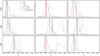 |
Fig. A.1. Artificial photometric (red vertical lines; Sect. 3.3), external spectroscopic (black vertical lines) and spectroscopically-calculated maximum (blue dotted vertical lines; Sect. 3.1) redshifts of 9 galaxies in GAMA. The realisations of GAMA spec-z, drawn from the conditional n(zspec. | zphot. ± 0.03) distribution surrounding each galaxy’s zphot., are displayed as black dashed histograms, and the corresponding zmax distribution is given in each panel as a blue dotted histogram. One sees that errors in photo-z (red vs. black vertical lines) and the corresponding inferred zmax (peaks of blue histograms vs. blue vertical lines) are compensated by the draws from n(zspec. | zphot.) and resulting zmax distributions. |
The utility of zph-randoms is most clearly demonstrated in Fig. A.2, where we compare the IA and clustering signals measured with our artificial GAMA photo-z to those measured with spectroscopic redshifts. The top-panels show the IA signals wg+, with the clustering wgg given in the bottom-panels. Each clustering signal is shown in ratio to the spectroscopic signal, whilst IA signals are simply overlain due to their low signal-to-noise. The 1σ jackknife errors (see Johnston et al. 2019, for details) for the spectroscopic signals are given by the shaded regions. The various scenarios of uniform or dynamic Π-binning (Sect. 4.1), and standard or zph-randoms, are indicated in the legend. One sees that both the binning and the choice of randoms are highly consequential for the clustering measurements, with the dynamic Π-bins and zph-windowed randoms (red circles) best recovering the shape of the clustering correlation function, and its amplitude to well within the spectroscopic error (at least for the total and blue samples) – residual disagreements in amplitude should be easier to accommodate with photo-z modelling, compared with large differences in shape arising due to redshift outliers. The IA signal is clearly more difficult to recover with fidelity, likely due to the characteristically low signal-to-noise of these correlations and their easy erasure by photo-z scatter.
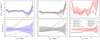 |
Fig. A.2. Attempted recoveries of all red (right), blue (left) and total (middle) sample correlations measured in our mock photo-z GAMA galaxy sample under various randoms and Π-binning scenarios (Sects. 3.3 and 4.1), with IA signals compared directly (top), and clustering signals shown in ratio (bottom), to the equivalent spectroscopic signals (dashed lines). 1σ jackknife errors (see Johnston et al. 2019) are indicated by shading. One sees that the dynamic binning in Π (circles) recovers much of the non-zero IA and clustering signal lost due to photo-z scatter (triangles), and that the use of zph-randoms (dot-dashed) and windowing (filled points) further aids in recovering the shape of the clustering signal, concerns with respect to amplitudes notwithstanding. |
Having tested our photo-z treatment with mock GAMA samples, we had to decide which combination of methods to apply to measurements of equivalent signals in PAUS. We computed the projected IA and clustering signals for every permutation of the following choices:
-
Colour-split: samples defined according to LEPHARE, CIGALE 2-cluster, or CIGALE 3-cluster (Fig. 3);
-
Π-binning: ‘standard’, uniform bins, or dynamic (adapted Fibonacci sequence; Sect. 4.1) bins;
-
Randoms: unwindowed, windowed, zph-unwindowed, or zph-windowed;
-
Photo-z selection: best 50% on Qz parameter (Fig. 7), or no selection,
for a total of 48 configurations. Displaying all of these, often similar, correlations poses difficulties for meaningful comparison, hence we elect to summarise the statistics in the following figures.
For projected IA signals wg+(rp) [and systematics-tests wg×(rp)], we display the significance of non-zero detection (computed with the full jackknife covariance12) in the range 0.1 < rp < 18 h−1 Mpc, where we are able to compute reliable jackknife errors for the PAUS W3 area – see Sect. 4.3. This IA summary is displayed in Fig. A.3, where one sees that we make no significant detection of systematics indicated by the position-shear correlation cross-component wg×, and that several configurations yield red galaxy alignment signals exceeding 2σ in signifance, with the most significant detection at 3.1σ. The three columns in this figure indicate the colours used to define red and blue galaxy samples, as given by the column-title. The top row gives wg+ correlations, with wg× systematics-tests on the bottom. Different correlation configurations are indicated at the bottom of the figure, with reference to Π-binning choices (‘dyn’-amic, or ‘unif’-orm), randoms choices (Unwindowed, Windowed, zph-Unwindowed, or zph-Windowed), and photo-z selection (selected on Qz, or not).
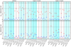 |
Fig. A.3. Summary of the significance of projected intrinsic alignment signal detection (given as xσ) in PAUS W3, with radial alignment component wg+ on the top row and cross-component (systematics-test) wg× on the bottom. Significances are computed in the range 0.1 < rp < 18 h−1 Mpc using full jackknife covariances (Sect. 4.3). Red and blue galaxy correlations are denoted by marker colours. The 3 columns show results for our different schemes of sample colour-splitting. Labels on the x-axis give the remaining specifics of each correlation configuration; ‘U’ (‘W’) denotes unwindowed (windowed) randoms. For ease of comparison, cyan forward-slash hatching indicates setups using zph-randoms (Sect. 3.3), and back-slashes indicate dynamic Π-binning (as opposed to uniform binning; no back-slashes). Grey shading denotes correlations measured on the best 50% of galaxies by photo-z quality (selected on the Qz parameter). We mark confidence levels 2σ and 3σ with horizontal lines. One sees that several correlation configurations yield red galaxy alignment signals reaching ∼2 − 3σ in significance. We make no significant detections of blue galaxy alignments, or systematics-test correlations, in the PAUS W3 data. |
One sees generally stronger wg+ correlations for red galaxies defined with the LEPHARE colour-split (see Fig. 3), though all red wg+ signals exceed their blue counterparts in significance. Importantly, the significance of any wg+ detection for blue galaxies is always negligible, at ≲0.8σ in all cases; modulo the impact of photo-z signal suppression (which will be elucidated in a future analysis using all of the PAUS area), we have reaffirmed the literature findings of negligible alignments between blue galaxies and the galaxy density field, now for a fainter flux-limited sample of blue galaxies than has previously been considered (see Mandelbaum et al. 2011; Tonegawa et al. 2018; Johnston et al. 2019).
For projected galaxy clustering signals, a meaningful comparison between correlation configurations is tricky, as we always expect significant detections due to the nature of the clustered galaxy distribution. Here, we perform non-linear least squares fits of simple, 2-parameter power laws of the form
 (A.1)
(A.1)
to the clustering signals, again in the range 0.1 < rp < 18 h−1 Mpc. The free parameters in the fit are the amplitude A at rp = 1 h−1 Mpc, and the power law slope γ, and we again make use of the full jackknife covariance for the fit. We display the fitted parameters for each of our 48 correlation configurations, and analogous fits (same scale-cuts) made to the spectroscopic GAMA signals, in Fig. A.4. Rows here give the different colour-split choices, with columns separating red (left) and blue (right) clustering fits. The remaining choices (Π-binning, randoms, photo-z selection) are indicated by markers and colours, as detailed in the legend, and GAMA fits are shown as gold stars with red or blue edges. In general, we see steeper power laws for red galaxy clustering, with respect to GAMA, and typically lower amplitudes at rp = 1 h−1 Mpc. Conversely, we find flatter power laws for blue galaxies, and that the fitted amplitudes are sensitive to our choices of Π-binning (dynamic bins → larger amplitude) and photo-z selection (best 50% Qz → larger amplitude).
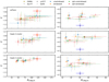 |
Fig. A.4. Comparison of projected clustering signal measurements in PAUS W3 and in spectroscopic GAMA data, summarised as fits of the simple, 2-parameter (amplitude A at rp = 1 h−1 Mpc, and slope γ) power law given by Eq. (A.1). Fits are made via the non-linear least squares method, in the range 0.1 < rp < 18 h−1 Mpc, and using full jackknife covariances (Sect. 4.3). All measured clustering signals feature heavily correlated rp-scales, sometimes resulting in poor goodness-of-fit, thus these points should be taken with moderation. Red (blue) galaxy correlations are shown in the left-hand (right-hand) column, with GAMA correlations given by gold stars with red (blue) outlines. PAUS correlations from each of our various configurations (changing Π-binning, randoms and photo-z selection) are denoted by markers and colours, as indicated by the legend. |
We elected to display, in Fig. 15, PAUS signals split by LEPHARE colours, for the dynamic Π-bins and zph-windowed randoms setup favoured in testing with the mock GAMA sample. For clustering in particular, these signals should be closer to the inaccessible (spectroscopic) truth, provided that (i) our mock photo-z are sufficiently PAUS-like, and (ii) the differences between PAUS/GAMA sample characteristics (area, depth, galaxy properties; see also Fig. 4) are not too impactful. Potential weaknesses in these assumptions include that (i) PAUS photo-z performance correlates somewhat with galaxy type, which we do not attempt to account for, and that (ii) the survey targets fainter objects at higher redshifts. We shall explore the robustness of our assumptions here in future work.
We choose to display the LEPHARE correlations due to the seemingly more discriminatory – and GAMA-esque – colour distribution inferred by LEPHARE, as compared with CIGALE (Fig. 3). Indeed, the higher significance of wg+ signals measured in red galaxy samples thus defined (Fig. A.3) is encouraging; from the intrinsic alignments literature, we have very good reason to expect a radial alignment of these galaxies with the density field (Mandelbaum et al. 2006a; Hirata et al. 2007; Joachimi et al. 2011; Samuroff et al. 2019; Johnston et al. 2019; Georgiou et al. 2019b). We reason then that our CIGALE colour classification scheme is not yet able to identify red galaxies as efficiently as the simple cut defined upon the LEPHARE colour-magnitude plane (Fig. 3). Forthcoming work will investigate further, and present finalised analyses of PAUS with CIGALE (Siudek et al., in prep.).
With our chosen setup, we made our most significant detection of red galaxy alignments in PAUS W3, at 3.1σ. The many tentative detections shown in Fig. A.3, and the suppression of IA in our mock photo-z signals (Fig. 15; top-left, open circles vs. downward triangles), suggest that a stronger signal may be present and washed-out by photo-z errors. We display Qz-selected sample correlations in Fig. A.5 for the same randoms/binning setup as in Fig. 15, noting the poor signal-to-noise for IA measurements. Moreover, the blue galaxies in PAUS are intrinsically fainter than in GAMA (Fig. 4), such that the higher observed amplitude of clustering is unlikely. It may be that our dynamic Π-binning is unsuitable for these more secure redshifts, though more investigation is required. A forthcoming analysis will extend our methods to the full PAUS area, making use of the latest photo-z and exploring the potential for more accurate recovery of photo-z-suppressed two-point correlations.
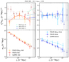 |
Fig. A.5. Same as Fig. 15, but swapping the mock photo-z GAMA signals out for a comparison with signals from the best 50% of PAUS photo-z according to the Qz parameter (denoted by ‘Qz50’ in the legends, and open-star data-points). Increases in noise and clustering amplitudes are evident when selecting on photo-z quality in this way. |
All Tables
All Figures
|
Fig. 1. Distribution of galaxies in the PAUS W3 field, with points coloured according to the log of each galaxy’s Qz value – this quantity describes the quality of photometric redshift estimation (low Qz = high photo-z quality) through a combination of the goodness-of-fit of SED templates to narrow-band photometry, and the shape of the resulting redshift probability density function; see Sects. 2.2 and 2.6. Circular holes in the footprint correspond to masks around foreground stars, with the largest gap (top-right) covering the Pinwheel Galaxy (Messier 101). |
| In the text | |
|
Fig. 2. Hexagonally-binned 2D histogram of PAUS W3 galaxies’ i-band k-corrections from redshift z (x-axis) to z = 0 – we assembled these by redshifting each galaxy’s best-fit SED model over the entire z-range, and taking ratios (Eq. (1)) of fluxes to the z = 0 flux. Cells are coloured by the count of galaxies resident in each cell. Solid coloured lines give the running-medians of k0(z) for five rest-frame colour bins, for which the average colours ⟨u − i⟩ are given in the legend (absolute magnitudes estimated with LEPHARE). |
| In the text | |
|
Fig. 3. Top-left: absolute rest-frame colour u − i vs. i magnitude for PAUS galaxies in the W3 area. These rest-frame magnitudes were derived for CFHTLenS (Erben et al. 2013) using the LEPHARE software package (Arnouts et al. 1999; Ilbert et al. 2006). We define the red sequence as those galaxies for whom u − i > 1.138 − 0.038i, as indicated by the orange line. Top-middle: spectroscopic redshift distribution of galaxies in GAMA, and photo-z distribution of PAUS W3, coloured according to the cuts in the top-left and top-right panels – we note that PAUS samples are restricted to 0.1 < zphot. < 0.8 for our correlation function analysis. Top-right: absolute rest-frame colour u − i vs. i magnitude for GAMA equatorial galaxies from the final GAMA data-set (Liske et al. 2015). We followed Johnston et al. (2019) in setting the red/blue boundary at rest-frame g − r = 0.66, and plot the galaxies on the u − i vs. i plane for comparison with PAUS W3. Bottom: CIGALE-estimated absolute rest-frame u − i vs. i for PAUS W3, with 2-cluster (left) and 3-cluster (right) galaxy type classification. |
| In the text | |
|
Fig. 4. Apparent (observed) and absolute i-band magnitudes of galaxies in PAUS (solid lines; limited to 0.1 < zphot < 0.8 and apparent i > 18) and GAMA (shading), with colours reflecting the (LEPHARE) red/blue selections displayed in Fig. 3 (top-left panel). We also display the magnitude distributions for 2 subsets of PAUS: (i) the best 50% selected on photo-z quality parameter Qz (dashed), and (ii) with apparent r < 19.8 (dotted) – approximately matching the GAMA flux-limit. Each histogram is individually normalised to unit area under the curve. Whilst the red galaxies in PAUS/GAMA are fairly similarly distributed in absolute i-band magnitude, PAUS exhibits a higher fraction of intrinsically faint blue galaxies. PAUS absolute magnitudes shown here are those computed using LEPHARE. |
| In the text | |
|
Fig. 5. Best fit parameters αj as a function of seeing. These parameters are used to estimate the multiplicative bias as a function of galaxy size and signal-to-noise ratio. |
| In the text | |
|
Fig. 6. Multiplicative bias μ as a function of seeing for simulated galaxies with 20 < i < 22.5. The red points correspond to the KSB estimates, which are significantly biased and depend upon image quality. The corrected biases are shown as grey (per-galaxy bias correction) and black (seeing-averaged bias correction) points. The histogram shows the seeing distribution for the CFHTLS W3 data. |
| In the text | |
|
Fig. 7. Top: photo-z quality log(Qz) for ∼4k PAUS-DEEP2 matched galaxies, as a function of their spectroscopically determined redshifts zspec., with red and blue colours reflecting the LEPHARE classification of the galaxies (see Fig. 3, top-left panel). A smaller value of Qz indicates a higher-quality photo-z estimate. Bottom: PAUS photo-z estimates vs. DEEP2 spec-z, again coloured by galaxy classification. The 1-to-1 relation is shown in the bottom panel as a faint yellow dashed line. |
| In the text | |
|
Fig. 8. Hexagonally-binned 2D histogram of PAUS-DEEP2 matched galaxies’ photo-z error, normalised by their spectroscopic redshifts and as a function of their LEPHARE rest-frame colour u − i. Shading indicates the log-counts in each cell. For the best 50% of photo-z according to the Qz parameter, we display the 16th, 84th percentiles of the normalised photo-z error for red (blue) galaxies as solid red (blue) horizontal lines. Half the difference between the percentiles is quoted for each as σ68. Dashed lines and bracketed values of σ68 are then for the total sample. |
| In the text | |
|
Fig. 9. Top: photometric redshift distribution of PAUS W3 (black solid), with spectroscopic redshifts of the DEEP2-matched galaxies (grey dashed), overlain with the randoms’ n(z), generated with and without the windowing (Sect. 3.2) and photo-z (‘zph-randoms’; Sect. 3.3) approaches, as indicated in the legend. Bottom: density contrast Δ(z) (Eq. (13)) computed after the final iteration of clone dispersal for each set of randoms – for zph-randoms, the ratio ngal(z) / nrand.(z) (Eq. (13)) is computed against galaxy redshifts drawn from n(zspec. | zphot.) (see Sect. 3.3), such that ngal(z)≠n(zphot.) and Δ(z) / Nclone can be greater than unity where nrand.(z) > n(zphot.), e.g., at zphot. ∼ 1. Our zph-randoms methods yield smoother redshift distributions, more faithful to the available n(zspec.). Red vertical lines delimit the redshift range employed in our correlation function analysis. |
| In the text | |
|
Fig. 10. Photometric redshift distributions of PAUS W3 galaxies, split into (LEPHARE) red/blue samples (shaded histograms), along with the n(z) for red/blue clones in the windowed randoms (solid lines) and the unwindowed randoms (dashed lines). Randoms shown here are the ‘zph-randoms’ described in Sect. 3.3. Each histogram/curve is individually normalised to unit area. |
| In the text | |
|
Fig. 11. Redshift distributions of random clones zrand, whose parent galaxies are situated at photometric redshifts zgal. Top: unwindowed clones are scattered over the entire redshift range, depending on the brightness, and hence zmax, of parent galaxies. Bottom: for the windowed randoms, 71.5% of a galaxy’s random clones are scattered within a ±1σ symmetric volume, centred on the location of the parent galaxy [we display σ = 3 × 10⁶ (h−1 Mpc)3 randoms here, for a clearer illustration]. We note that the symmetry is in volume coordinates, hence in redshift/comoving coordinates the windows are extended in the direction of the observer, and slightly squashed in the outward direction. This figure is closely based on a similar plot presented by Farrow et al. (2015) for GAMA galaxies and randoms (their Fig. 3). Plateaus in the red curves, on approach to redshift zero, correspond to faint, very low-redshift galaxies which are excluded from our analysis. |
| In the text | |
|
Fig. 12. GAMA spectroscopic redshift distribution (top-panel; blue), overlaid with our approximately PAUS-like photometric redshift distribution (top-panel; red) – these photo-z are created by applying a redshift- and magnitude-dependent Gaussian scatter (middle-panel; Eq. (14)) to the spec-z, along with a probabilistic ‘kick’ (bottom-panel; Eq. (15)) to generate catastrophic outliers, and a manual relocation of some galaxies to zphot. ∼ 0.27 (see Sect. 3.3). Bottom-panels are hexagonally-binned 2D histograms, with cells coloured according to the mean GAMA spec-z of objects residing in each cell. |
| In the text | |
|
Fig. 13. Contours depicting cumulative population fractions 0.08, 0.25, 0.42, 0.58, 0.75 and 0.92 for GAMA galaxy/zph-randoms catalogues on the zphot./rand. vs. zspec. plane, where the y-axis refers to zphot. for galaxies and zrand. for randoms. For randoms, zspec. refers to the spectroscopic redshift of the parent galaxy to a clone at redshift zrand.. Blue contours depict our windowed randoms, with window-width σ = 5 × 10⁶ (h−1 Mpc)3, and orange contours are for unwindowed randoms. One clearly sees the intentional photo-z biases (Sect. 3.3) in the galaxy contours (solid black), and how the randoms (dashed colours) softly mimic them. Figure 14 shows five ‘marginals’ through this distribution for (zph-windowed randoms only), collapsing the y-axis to show n(zspec. | zphot.). |
| In the text | |
|
Fig. 14. Spectroscopic redshift distributions of GAMA galaxies, binned by the mock photometric redshifts we describe in Sect. 3.3. Vertical black lines depict the bin-edges in zphot. and solid curves give the resulting n(zspec. | zphot.) for galaxies. Selecting only the clones of those binned galaxies, from our ‘zph-windowed’ GAMA randoms [σ = 5 × 10⁶ (h−1 Mpc)3], the randoms’ redshift distributions are then given by the dashed curves. One sees that our ‘zph-randoms’ [generated using samples from the n(zspec. | zphot.)’s centred on individual galaxies’ zphot. – see Sect. 3.3] are thus able to trace the artificial photo-z biases – for example, the secondary peak at z ∼ 0.3 in the final panel, which is captured by the tail of the randoms’ n(z). These curves are equivalent to horizontal bands in Fig. 13, summed over the y-axis. |
| In the text | |
|
Fig. 15. Projected position-shear (top) and position-position (bottom) correlations measured for red (left) and blue (right) galaxies in PAUS (filled pentagons) and GAMA (open circles and filled triangles). The PAUS correlations displayed here are for all galaxies (i.e. not selected according to Qz), split by colour according to LEPHARE, measured with zph-windowed randoms and dynamic Π-bins – see Appendix A for details on our choice here. Downward triangles display the correlations measured in GAMA using our mock photo-z, described in Sect. 3.3. Grey hatching indicates the larger scales where our PAUS W3 jackknife would yield unreliable errorbars (see Sect. 4.3). |
| In the text | |
|
Fig. A.1. Artificial photometric (red vertical lines; Sect. 3.3), external spectroscopic (black vertical lines) and spectroscopically-calculated maximum (blue dotted vertical lines; Sect. 3.1) redshifts of 9 galaxies in GAMA. The realisations of GAMA spec-z, drawn from the conditional n(zspec. | zphot. ± 0.03) distribution surrounding each galaxy’s zphot., are displayed as black dashed histograms, and the corresponding zmax distribution is given in each panel as a blue dotted histogram. One sees that errors in photo-z (red vs. black vertical lines) and the corresponding inferred zmax (peaks of blue histograms vs. blue vertical lines) are compensated by the draws from n(zspec. | zphot.) and resulting zmax distributions. |
| In the text | |
|
Fig. A.2. Attempted recoveries of all red (right), blue (left) and total (middle) sample correlations measured in our mock photo-z GAMA galaxy sample under various randoms and Π-binning scenarios (Sects. 3.3 and 4.1), with IA signals compared directly (top), and clustering signals shown in ratio (bottom), to the equivalent spectroscopic signals (dashed lines). 1σ jackknife errors (see Johnston et al. 2019) are indicated by shading. One sees that the dynamic binning in Π (circles) recovers much of the non-zero IA and clustering signal lost due to photo-z scatter (triangles), and that the use of zph-randoms (dot-dashed) and windowing (filled points) further aids in recovering the shape of the clustering signal, concerns with respect to amplitudes notwithstanding. |
| In the text | |
|
Fig. A.3. Summary of the significance of projected intrinsic alignment signal detection (given as xσ) in PAUS W3, with radial alignment component wg+ on the top row and cross-component (systematics-test) wg× on the bottom. Significances are computed in the range 0.1 < rp < 18 h−1 Mpc using full jackknife covariances (Sect. 4.3). Red and blue galaxy correlations are denoted by marker colours. The 3 columns show results for our different schemes of sample colour-splitting. Labels on the x-axis give the remaining specifics of each correlation configuration; ‘U’ (‘W’) denotes unwindowed (windowed) randoms. For ease of comparison, cyan forward-slash hatching indicates setups using zph-randoms (Sect. 3.3), and back-slashes indicate dynamic Π-binning (as opposed to uniform binning; no back-slashes). Grey shading denotes correlations measured on the best 50% of galaxies by photo-z quality (selected on the Qz parameter). We mark confidence levels 2σ and 3σ with horizontal lines. One sees that several correlation configurations yield red galaxy alignment signals reaching ∼2 − 3σ in significance. We make no significant detections of blue galaxy alignments, or systematics-test correlations, in the PAUS W3 data. |
| In the text | |
|
Fig. A.4. Comparison of projected clustering signal measurements in PAUS W3 and in spectroscopic GAMA data, summarised as fits of the simple, 2-parameter (amplitude A at rp = 1 h−1 Mpc, and slope γ) power law given by Eq. (A.1). Fits are made via the non-linear least squares method, in the range 0.1 < rp < 18 h−1 Mpc, and using full jackknife covariances (Sect. 4.3). All measured clustering signals feature heavily correlated rp-scales, sometimes resulting in poor goodness-of-fit, thus these points should be taken with moderation. Red (blue) galaxy correlations are shown in the left-hand (right-hand) column, with GAMA correlations given by gold stars with red (blue) outlines. PAUS correlations from each of our various configurations (changing Π-binning, randoms and photo-z selection) are denoted by markers and colours, as indicated by the legend. |
| In the text | |
|
Fig. A.5. Same as Fig. 15, but swapping the mock photo-z GAMA signals out for a comparison with signals from the best 50% of PAUS photo-z according to the Qz parameter (denoted by ‘Qz50’ in the legends, and open-star data-points). Increases in noise and clustering amplitudes are evident when selecting on photo-z quality in this way. |
| In the text | |
Current usage metrics show cumulative count of Article Views (full-text article views including HTML views, PDF and ePub downloads, according to the available data) and Abstracts Views on Vision4Press platform.
Data correspond to usage on the plateform after 2015. The current usage metrics is available 48-96 hours after online publication and is updated daily on week days.
Initial download of the metrics may take a while.