| Issue |
A&A
Volume 699, July 2025
|
|
|---|---|---|
| Article Number | A273 | |
| Number of page(s) | 18 | |
| Section | Galactic structure, stellar clusters and populations | |
| DOI | https://doi.org/10.1051/0004-6361/202452614 | |
| Published online | 16 July 2025 | |
The completeness of the open cluster census towards the Galactic anticentre
1
Landessternwarte, Zentrum für Astronomie der Universität Heidelberg,
Königstuhl 12,
69117
Heidelberg,
Germany
2
Max-Planck-Institut für Astronomie,
Königstuhl 17,
69117
Heidelberg,
Germany
3
Departament de Física Quàntica i Astrofísica (FQA), Universitat de Barcelona (UB),
Martí i Franquès, 1,
08028
Barcelona,
Spain
4
Institut de Ciències del Cosmos (ICCUB), Universitat de Barcelona (UB),
Martí i Franquès, 1,
08028
Barcelona,
Spain
5
Institut d’Estudis Espacials de Catalunya (IEEC),
Edifici RDIT, Campus UPC,
08860
Castelldefels (Barcelona),
Spain
6
INAF, Osservatorio Astrofisico di Arcetri,
Largo E. Fermi 5,
50125
Firenze,
Italy
7
Dipartimento di Fisica e Astronomia, Università di Padova,
Vicolo dell’Osservatorio 3,
35122
Padova,
Italy
8
Leiden Observatory, Leiden University,
Einsteinweg 55,
2333
CC Leiden,
The Netherlands
9
Institute of Astronomy, University of Cambridge,
Madingley Road,
Cambridge
CB3 0HA,
UK
10
School of Physics and Astronomy, Monash University,
Clayton,
VIC 3800,
Australia
11
Centre of Excellence for Astrophysics in Three Dimensions (ASTRO-3D),
Melbourne,
Victoria,
Australia
12
Center for Computational Astrophysics, Flatiron Institute,
162 Fifth Ave,
New York,
NY
10010,
USA
13
INAF, Osservatorio Astrofisico di Torino,
Strada Osservatorio 20,
Pino Torinese
10025,
Torino,
Italy
★ Corresponding authors: This email address is being protected from spambots. You need JavaScript enabled to view it.
Received:
15
October
2024
Accepted:
12
June
2025
Abstract
Context. Open clusters have long been used as tracers of Galactic structure. However, without a selection function to describe the completeness of the cluster census, it is difficult to quantitatively interpret their distribution.
Aims. We create a method to empirically determine the selection function of a Galactic cluster catalogue. We test it by investigating the completeness of the cluster census in the outer Milky Way, where old and young clusters exhibit different spatial distributions.
Methods. We develop a method to generate realistic mock clusters as a function of their parameters, in addition to accounting for Gaia’s selection function and astrometric errors. We then inject mock clusters into Gaia DR3 data, and attempt to recover them in a blind search using HDBSCAN.
Results. We find that the main parameters influencing cluster detectability are mass, extinction, and distance. Age also plays an important role, making older clusters harder to detect due to their fainter luminosity function. High proper motions also improve detectability. After correcting for these selection effects, we find that old clusters are 2.97 ± 0.11 times more common at a Galactocentric radius of 13 kpc than in the solar neighbourhood - despite positive detection biases in their favour, such as hotter orbits or a higher scale height.
Conclusions. The larger fraction of older clusters in the outer Galaxy cannot be explained by an observational bias, and must be a physical property of the Milky Way: young outer-disc clusters are not forming in the outer Galaxy, or at least not with sufficient masses to be identified as clusters in Gaia DR3. We predict that in this region, more old clusters than young ones remain to be discovered. The current presence of old, massive outer-disc clusters could be explained by radial heating and migration, or alternatively by a lower cluster destruction rate in the anticentre.
Key words: methods: data analysis / Galaxy: disk / Galaxy: evolution / open clusters and associations: general
© The Authors 2025
 Open Access article, published by EDP Sciences, under the terms of the Creative Commons Attribution License (https://creativecommons.org/licenses/by/4.0), which permits unrestricted use, distribution, and reproduction in any medium, provided the original work is properly cited.
This article is published in open access under the Subscribe to Open model. This email address is being protected from spambots. You need JavaScript enabled to view it. to support open access publication.
1 Introduction
Star clusters are groups of a dozen to hundreds of thousands of coeval stars, born from the collapse of the same parent molecular cloud (Portegies Zwart et al. 2010). Stars in a cluster can remain gravitationally bound to their siblings for billions of years. Systematic searches for star clusters were a popular activity in early modern astronomy (e.g. Messier 1781; Herschel 1786, 1789). Since their main parameters (in particular age and distance) can be estimated more reliably than for individual stars, they have long been used as tracers of the structure and overall properties of the Milky Way (e.g. Trumpler 1930; Janes & Adler 1982).
Open clusters (OCs) are the most common type of star cluster in the Milky Way, with typical ages no greater than a few hundred million years (Cantat-Gaudin 2022) and masses ranging from less than a hundred to no larger than a few thousand solar masses (Almeida et al. 2023; Hunt & Reffert 2024; Almeida et al. 2025).
Catalogues of stellar proper motions have enabled the identification of OCs as co-moving groups (Alessi et al. 2003; Kharchenko et al. 2005; Froebrich et al. 2007), but we remark that until recently the vast majority of the objects listed in the most widely used cluster databases (Dias et al. 2002; Netopil et al. 2012; Kharchenko et al. 2013) were discovered as simple spatial overdensities in on-sky positions. The ESA Gaia mission (Gaia Collaboration 2016) has transformed our ability to study stellar populations in the Milky Way (Brown 2021), and its second (Gaia Collaboration 2018) and third data releases (Gaia Collaboration 2021b) have enabled the discovery of thousands of new OCs1 in the 5D space of positions, proper motions, and parallaxes, in addition to validation with Gaia’s three-colour photometry (e.g. Castro-Ginard et al. 2018; Cantat-Gaudin et al. 2019; Castro-Ginard et al. 2020; Hunt & Reffert 2023).
While the most recent cluster catalogues feature unprecedented numbers of objects characterised to a high level of precision, we still have a poor understanding of the completeness of the cluster census. It feels intuitive that massive and nearby clusters are easier to detect than small and distant objects. Allsky blind searches performed on the Gaia catalogue are also likely to be biased in favour of clusters with proper motions different to their background field, and to be more efficient at recovering clusters in sparser regions of the sky than in crowded fields. The issue of completeness dropping with distance is often sidestepped in astronomy by restricting studies to a volume within which the authors consider the sample is near 100% complete (e.g. Koposov et al. 2008; Kharchenko et al. 2013; Hunt & Reffert 2024). This approach is in general highly sub-optimal (Rix et al. 2021).
Rather than artificially restricting catalogues to create volume-complete samples, we should strive to construct their selection function: a quantitative description of completeness as a function of location and other relevant parameters. A selection function allows one to account for selection effects in the incomplete regime, thus enabling studies of the Milky Way on a much larger scale. Even assuming that catalogues are complete within a certain volume, the selection function is a critical piece of information to extend studies beyond the solar neighbourhood, or to compare the Milky Way to other galaxies in an unbiased way. To our knowledge, the only study attempting to establish a selection function for the cluster census was performed by Anders et al. (2021) for the Gaia DR2 cluster catalogue of Cantat-Gaudin et al. (2020), which itself exploited a completeness experiment conducted by Castro-Ginard et al. (2020) using Cantat-Gaudin et al. (2018) as a reference catalogue.
The present paper focuses on the spatial and age distribution of clusters in the outer Milky Way, in the direction of the Galactic anticentre (140° ≤ l ≤ 220°), as well as an additional region where the Galactic warp appears most strongly in the cluster population (220° < l < 240°). While young clusters (defined in this study as younger than log t = 8.5) are six times more numerous than old clusters within 11 kpc of the Galactic centre, old clusters are twice as numerous beyond 11 kpc. Figure 1 shows that the number of known young clusters decreases more quickly with Galactocentric distance than for older objects. The distant outer-disc clusters are also mostly found in the third Galactic quadrant. Without a quantitative selection function, we cannot know whether this distribution is a physical property of the Milky Way or the result of a biased cluster census.
In this study, we inject mock clusters into Gaia data, and we attempt to recover them in a blind search akin to typical cluster searches. We aim to develop a method applicable to any cluster blind search in the Gaia era, and demonstrate it in use on the Galactic anticentre. This paper is structured as follows. Section 2 outlines the choice of catalogue and cluster retrieval method that we aim to establish a selection function for. Next, Sect. 3 presents our approach to generating mock clusters and detecting them in the Gaia data. Section 4 presents the results of our search and the selection function we build from this experiment. Section 5 discusses the consequences of the recovered completeness estimates on our understanding of Galactic structure as traced by OCs. Finally, Sect. 6 summaries our findings and provides a brief outlook to future work.
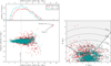 |
Fig. 1 Spatial distribution of high-certainty clusters (CST>4) from Hunt & Reffert (2023). Ages are taken from Cavallo et al. (2024) as they are more accurate for old clusters (see Sect. 2 for discussion). Top left: histogram of cluster galactocentric radii divided into young (log t < 8.5, blue) and old (log t > 8.5, red) clusters and with a 200 pc bin width. Bottom left: distribution of the same young and old clusters but in terms of altitude Z and Galactocentric radius RGC, assuming RGC,⊙ = 8.2 kpc. Bottom right: projection of these clusters in heliocentric Galactic co-ordinates, with the Sun located at (X,Y) = (0,0). The dotted lines indicate Galactocentric radii from 10 to 18 kpc. The shaded area is the region investigated in this study (140° ≤ ℓ ≤ 240° starting 2 kpc from the Sun). In both lower panels, the cross indicates the cluster Saurer 1, visible in Gaia data but not recovered in the blind search of Hunt & Reffert (2023). |
2 Cluster sample
The current cluster census includes multiple different catalogues and individual cluster searches generated with Gaia data releases, often using a wide range of different methodologies (see Introduction). For the purposes of this work, we aim to establish the selection function of OCs in the Hunt & Reffert (2024) (hereafter HR24) catalogue, as it is a recently developed catalogue based on the latest Gaia data release (DR3) that also includes parameters determined for all objects. Nevertheless, establishing the selection function of the HR24 catalogue is not without some complications that we discuss in this section. As HR24’s cluster list is an updated version of the Hunt & Reffert (2023) (hereafter HR23) catalogue, construction of the HR24 catalogue hence involved a number of steps that must be replicated to establish its full selection function, which we discuss below.
HR24 is based on a cluster search performed in HR23. HR23 applied the Hierarchical Density-Based Spatial Clustering of Applications with Noise (HDBSCAN, Campello et al. 2013; McInnes et al. 2017) algorithm to recover star clusters from Gaia DR3, recovering a total of 7167 clusters. To augment the HDBSCAN algorithm, as it often produces a high number of false positives when applied to Gaia data, they used the cluster significance test (CST) developed in Hunt & Reffert (2021), which measures the statistical significance of a candidate cluster compared to its immediate surroundings. To remove unreliable clusters and likely false positives, HR23 includes only 7167 cluster candidates with CST > 3σ, which is the minimum bar that a cluster must pass to be included in HR23 or HR24.
Where the two catalogues differ is in their definition of an OC. HR23 found that HDBSCAN was sensitive to other types of star cluster than simply OCs, with their catalogue including over 100 globular clusters and a large number of clusters that appeared to be unbound moving groups, particularly in the region close to the Sun. Classification of globular clusters was performed with comparison to the literature. To classify OCs and moving groups, HR23 used the statistical cuts on cluster radius and proper motion dispersion defined in Cantat-Gaudin & Anders (2020); however, they found that these cuts appeared to be insufficient for many more compact moving groups. Hence, HR24 introduced a method based on cluster mass and radius, classifying 1309 clusters from HR23 as moving groups. In practice, in our studied region in the anticentre and at distances greater than 2 kpc, the differences between the two catalogues are minor: only an additional 18 out of 856 clusters in our region are classified as moving groups in HR24, in addition to one extra globular cluster (see Table 1). Almost all of these moving groups are removed with a more stringent cut on CST of 5σ. For the purposes of this work, we use only the sample of clusters in HR24 classified as OCs (Type = o), although future work on selection functions near to the Sun (where the moving group fraction is higher) may also need to additionally calculate the probability that a true OC was correctly classified as one by the HR24 pipeline.
It is also worth noting that HR23 and HR24 include a ‘high quality’ cluster sample. HR23 used a neural network to classify cluster colour-magnitude diagrams (CMDs) and assign them a quality QCMD between zero and one, and they recommended some analyses instead use a more strongly cut high quality cluster sample: defined as clusters with CST > 5σ and QCMD > 0.5. In this work, we do not establish the selection function of their high quality cluster sample, as this would be difficult to do fairly: given that their CMD classifier was trained on simulated clusters and then applied to real clusters, and was around three times more accurate at classifying simulated clusters than real clusters, it is likely that presenting their CMD classifier with our simulated clusters would strongly overestimate the probability that a real cluster has a good CMD class. Nevertheless, the selection function of the HR23 cluster classifier could still be worthwhile to explore in a future work.
Finally, it is also worth commenting on the sample of cluster ages that we adopt. Cavallo et al. (2024) used a machine learning method to fit isochrones to clusters in HR23. They found that cluster ages can be underestimated for the oldest clusters in HR23 (and by extension HR24, which contains the same age parameters). For this work, as we are interested particularly in old clusters, we use only the Cavallo et al. (2024) cluster ages and extinctions for HR24 clusters in our analysis and figures.
Number of clusters in our studied region in HR23 and HR24 given multiple possible cuts.
3 Methods for creating an empirical OC selection function
In this section, we describe all steps in our methodology to calculate an empirical cluster selection function. Firstly, we describe how we simulated realistic clusters. Next, we describe the process of injecting and retrieving them in a manner similar to that in HR23. Finally, we discuss how we post-processed these results to create a smooth cluster selection function.
3.1 Creation of simulated clusters
To derive a robust selection function of the OC census using retrieval of simulated clusters, it is essential that our simulated clusters are as realistic as possible. Hence, the first step in our method was the development of a robust simulated cluster generation pipeline.
There are a number of parameters that must be chosen to create a Gaia observation of a simulated cluster, which we discuss in the following sections. Some of these parameters are intrinsic (selected during this study), and some of them are extrinsic (such as properties of Gaia observations). The intrinsic parameters of a simulated cluster are: its position, which we quantify in Galacto-centric co-ordinates l and b as well as its distance from the Sun d; its total mass, M, with a corresponding number of stars N sampled from an assumed mass function of the cluster; the structure of the cluster, defined by a King (1962) profile; the current velocity of the cluster, defined as its proper motions μα* and μδ, as well as its radial velocity; the velocity dispersion of the cluster’s member stars, σ1D; the cluster’s age, log t; and its metallicity, [Fe/H]. The extrinsic parameters of a cluster are: the assumed mean extinction AV of the cluster; the distribution of Gaia photometric and astrometric uncertainties at the cluster’s position; the selection function of the Gaia satellite and the subsample of Gaia data analysed in HR23 at the cluster’s position, causing many member stars to be missing from the analysed dataset; and the resolving power of Gaia, which causes some multiple star systems to be resolved as a single source. Having selected intrinsic parameters for a given cluster, creation of simulated clusters involves two steps: firstly, generation of cluster member star photometry; and secondly, generation of cluster member star astrometry.
3.1.1 Simulation of member star photometry
To generate mock photometry for a given cluster age, metallicity, and total mass, we began by sampling the masses of its member stars from a Kroupa (2001) initial mass function using the Python package IMF2. We then assigned the stars an absolute Gaia DR3 G, GBP, and GRP-band magnitude using version 1.2S PARSEC isochrones (Bressan et al. 2012; Chen et al. 2014; Tang et al. 2014; Chen et al. 2015).
We randomly picked a location for each cluster, with a Galactic longitude l between 140° and 240°, Galactic latitude b between −10° and +10°, and a heliocentric distance d between 2 and 15 kpc, sampled uniformly within these ranges. We then assigned interstellar extinction to the cluster based on the value reported in the 3D dust map of Green et al. (2019) at its location.
Having applied foreground extinction to our cluster member stars, we simulated additional extrinsic effects on them. Firstly, we simulated the chance that a star is in a binary system using the unresolved binary star correction code of HR24. In brief, this method takes all simulated stars for a given cluster, and iteratively pairs them into binaries based on primary massdependent binarity probabilities from Moe & Di Stefano (2017). Then, the average separation between the host and orbiting star from Moe & Di Stefano (2017) was used to estimate whether Gaia would resolve the system as a resolved or unresolved, and hence whether or not to ‘merge’ the two sources into one. Some stars being in unresolved binary systems reduces the total number of sources observed by Gaia for a given cluster, and hence the detectability of the overall cluster is reduced (especially for low-mass clusters).
The next step was to simulate the probability that a given simulated star would be in the subsample of Gaia data analysed by HR23. To estimate the probability that a simulated star would even appear in the Gaia dataset initially, we compared its G-band magnitude to the Gaia selection function of Cantat-Gaudin et al. (2023) at the star’s position and magnitude, and rejected the star if a random uniform variable is greater than the corresponding value of the Gaia selection function. In practice, this removes many faint sources in our simulated clusters that are below Gaia’s magnitude limit, which is dependent on position and can be as faint as G ≈ 21.
However, HR23 analysed a subsample of Gaia data after applying quality cuts; incorporating a similar quality cut on our simulated clusters is important to ensure that they have the same number of stars and luminosity function as a real cluster in HR23, particularly at the faint end of the cluster (G & 18 mag) where HR23’s quality cuts have the largest impact. HR23 performed clustering only on Gaia sources with proper motions and parallaxes, as well as only those with G, GBP, and GRP photometry; in addition, they cut sources with low-quality astrometry with a Rybizki et al. (2022) v1 quality flag below 0.5. Simulating the reason why a given star may fail one or more of these cuts is complicated: reasons such as a source’s multiplicity, crowding, brightness, or colour could cause Gaia’s astrometric or photometric fitting to fail or produce a low-quality result (Lindegren et al. 2021; Riello et al. 2021). As an approximation, we calculated the subsample selection function of the HR23 cuts on Gaia with the method outlined in Castro-Ginard et al. (2023) and on a grid of HEALPix3 (Górski et al. 2005) level 6 pixels across our studied region in the Galactic anticentre, creating a selection function that depends on position and G-band magnitude. Then, for a given cluster, we applied the selection function in the HEALPix pixel they are in to the stars in the cluster based on their G-band magnitude. This approximation does not simulate when a certain combination of binary star orbital parameters causes a source to have low-quality astrometry with Gaia; however, it does capture the impact of crowding on the Gaia pipeline, and how faint sources often do not have proper motions and parallaxes - hence causing them to fail the HR23 quality cuts, reducing the number of stars at the faint end of clusters in HR23. Fora typical cluster in the anticentre, our approximate subsample selection function reduces the magnitude limit of our simulated clusters from G ~ 20.7 to G ~ 19.
For this study, we do not simulate further impacts on the photometry of our simulated clusters, such as Gaia photometric uncertainties - for similar reasons as to why we do not simulate differential reddening. We recall that our clustering algorithm only uses 5D astrometric measurements. Thus, we do not require fully realistic cluster CMDs, and only need stellar G-band magnitudes to assign astrometric errors to stars in the following section. The uncertainties on G-band magnitudes are small enough to be insignificant to this step.
3.1.2 Simulation of member star astrometry
To generate member star astrometry, we began by generating the 3D positions of stars in each cluster. We assumed that all clusters follow a King profile, parameterised by a core radius rc and a tidal radius rt. To select rt for each cluster, we assumed that all clusters fill their Roche lobe, with their tidal radius equalling their Jacobi radius; we hence calculated the expected tidal radius of each cluster based on their mass and the potential of the Milky Way. For the potential, we used the MWPotential2014 model in galpy4 (Bovy 2015), which models the potential of the Milky Way with a simple, smooth model, composed of a a bulge, disk, and dark matter halo. Then, the potential is used to calculate the cluster’s Jacobi radius (Eq. (2) in HR24). Given the weak cube root dependence of the cluster’s Jacobi radius on the components of the potential model, the choice of potential has a relatively small impact on our study. Next, for each cluster, we chose a core radius of the cluster rc (defining how concentrated a given cluster is), sampling uniformly from a distribution chosen later in this work. Having selected values for rc and rt, the 3D position of each star is then randomly sampled using the King profile sampler in ocelot5 (Hunt & Reffert 2021), which uses the equation for spatial density of a King profile (Eq. 27 in King 1962) and rejection sampling to sample random 3D co-ordinates given a King profile. These true positions were then converted to observed co-ordinates with parallaxes calculated as inverse distances by Astropy (Astropy Collaboration 2013, 2018, 2022).
Next, we generated the velocities of simulated cluster member stars, which begins by choosing an overall mean velocity for each cluster. In order to sample the full velocity space efficiently, we wish to sample all possible proper motions that clusters could reasonably have, which mostly includes proper motions corresponding to orbits reminiscent of stars in the thin disk where OCs mostly reside (Cantat-Gaudin 2022), but could also hypothetically include higher-velocity evolved thick disk-like orbits. As a simple method to sample realistic proper motions, we used the proper motion distribution of field stars in each clustering region at a similar parallax to that of the cluster to derive cluster mean proper motions, assuming that field star proper motions follow a Gaussian distribution and selecting only those with a parallax within 0.1 mas of a simulated cluster’s parallax. This method samples a wider range in proper motions than the proper motion distribution of known clusters (see Fig. B.1), ensuring that we can later experiment with how more or less extreme cluster proper motions can improve cluster detectability. For this study, we assumed that clusters have no radial velocities, as the impact of radial velocities on proper motions (perspective acceleration; Lindegren & Dravins 2021) is insignificant at the distances we consider in this work, as perspective acceleration only measurably impacts clusters that have a large on-sky distribution - generally only those within a few hundred parsecs.
Having chosen a cluster mean proper motion, we generated the cluster’s internal star-by-star dynamics by sampling the true 3D velocity of stars from a multivariate Gaussian distribution, with a dispersion given by the velocity dispersion equation in Portegies Zwart et al. (2010) (hereafter PZ10) and assuming that clusters are in virial equilibrium (i.e. the constant η in their equation equals ten). In practice, at the distances and cluster masses considered in this work, even for a highly supervirial cluster, the internal velocity dispersion within star clusters is smaller than Gaia proper motion uncertainties - for instance, a relatively high mass virialised 103 M Pleiades-like cluster at a distance of 5 kpc has an internal dispersion of just ~0.02 mas yr−1. Nevertheless, our pipeline includes internal cluster velocity dispersion in preparation for future work focusing on closer objects.
Finally, we sampled observed cluster member proper motions and parallaxes that include Gaia measurement uncertainties. Gaia astrometric uncertainties are principally a function of sky position and G-band magnitude (Lindegren et al. 2021; Fabricius et al. 2021). We used the data-driven approach of HR24 to calculate expected astrometric errors: in the field of analysed Gaia data around each cluster in this study, the nearest real star in G-band magnitude to a simulated star was chosen, and its measurement uncertainties were assigned to the simulated star. In the future, an approach that also uses GBP and GRP photometry may be more accurate. Sampling from a Gaussian distribution, these astrometric uncertainties were then added on to the true astrometry of each simulated star to create its mock Gaia observation.
3.2 Cluster blind search
3.2.1 Cluster recovery method
Using our simulated cluster generation pipeline, the next step in our method was to perform injection and retrieval of simulated clusters. We used the exact methodology from HR23 to retrieve the injected clusters, which we briefly outline here.
We began by dividing Gaia data into HEALPix level five pixels in a Galactic co-ordinate frame, performing clustering on each level five pixel (~3.4 deg2 in area) plus an overlap region of all eight neighbouring pixels surrounding it: hence, each clustering ‘field’ contains nine HEALPix level five regions. As we aim to fully replicate the steps involved in the clustering in HR23, we also applied the HR23 quality cuts on Gaia data, retaining only Gaia sources with proper motions, parallaxes, and photometry in the G, BP, and RP bands, in addition to cutting all stars with a Rybizki et al. (2022) v1 quality flag below 0.5. We found that inserting four simulated clusters per field per run (corresponding to a density of around one cluster per square degree) maximised the number of clusters we could simulate injections and retrievals of, but without causing the cluster density to be so high that simulated clusters overlapping was common.
Having inserted simulated clusters into a region, we ran HDBSCAN (Campello et al. 2013; McInnes et al. 2017) at four different min_cluster_size values (10, 20, 40, and 80), and with min_samples set to 10. Finally, for every detected cluster, we also computed its cluster significance test (CST) score (Hunt & Reffert 2021), which measures the statistical significance of a cluster against the surrounding field as a way to remove false positive clusters - effectively producing a signal to noise ratio of each cluster relative to the surrounding field. The HR23 study only retained clusters with CST ≥ 3σ; hence, we consider any cluster with a CST below this to be undetected in HR23. However, HR23 also recommended using a higher cut when higher quality cluster samples are desired (such as CST > 5σ), and so we also investigate the selection function of some higher CST cuts in this work when analysis of a higher quality sample is required.
The use of increasing min_cluster_size values was adopted by HR23 to deal with the fact that HDBSCAN sometimes splits large clusters into multiple subclusters. For the present study, whenever a given min_cluster_size leads to none of the clusters being split into multiple components, we terminated the clustering early. This can result in as much as a 75% speed-up in our methodology in cases in which all clusters would be detected (or non-detected) identically at all min_cluster_size values.
Figure 2 shows an example simulation and detection of a cluster, which includes realistic astrometric uncertainties and simulated Gaia selection effects. The cluster is young (log t = 7.4), has a total mass of 1412 M⊙, is at a distance of 5.2 kpc from the Sun, and has an extinction of AV = 3.1 mag. It should be noted that the CMD of the cluster is more ideal than for a real object: we did not simulate differential reddening and photometric uncertainties, as they do not affect our detection pipeline as it only uses astrometric data (see Sect. 3.1.1.) The simulated cluster contains 132 stars that would be visible in our subsample of the Gaia dataset if this cluster was real. Of these stars, only 83 are assigned as members of the cluster, with many (predominantly faint) stars with higher astrometric uncertainties not being identified as cluster members. In addition, 46 field stars that are nearby, unassociated parts of the Gaia dataset were erroneously assigned as cluster members. This example corresponds to a clear detection, with a CST of 16.2.
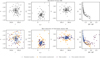 |
Fig. 2 Example result of the injection-recovery procedure for a simulated OC, in the typical projections used in cluster discovery studies. Top row: original simulated cluster (including realistic Gaia DR3-like astrometric errors), shown in position (far left), proper motion (centre left), position versus parallax (centre right), and the colour-magnitude diagram of the cluster (far right). This simulated cluster was then inserted into Gaia data to test the cluster recovery ability of HDBSCAN. Bottom row: same as top row, but for the best recovery from Gaia data of this cluster by HDBSCAN. True members of the cluster that were correctly assigned as members by HDBSCAN are shown as blue circles. Non-member field stars from the Gaia dataset that were incorrectly added to the cluster are shown as purple squares. Finally, member stars that HDBSCAN missed are shown as orange crosses. |
3.2.2 Explored cluster parameter space
Having defined a cluster simulation and recovery pipeline, our final step was to decide on clusters to simulate and run our full injection and retrieval experiment. We investigated ranges in cluster parameters that fully sample the range of observed cluster parameters in the Galactic anticentre, which are summarised in Table 2. For the purposes of this work, we fixed some parameters that have a minimal impact on our cluster detectability to reduce the size of our parameter space. Namely, we set cluster metallic-ity [M/H] = −0.2, as metallicity has a minimal impact on cluster CMDs and can be ignored; nevertheless, a value of −0.2 is still a fair average value for the Galactic anticentre (Spina et al. 2022; Carbajo-Hijarrubia et al. 2024). In addition, as our considered clusters are too distant for their velocity dispersion to have an impact on their measured proper motion dispersion, we assume clusters are virialised (i.e. η = 10) for this study.
Choosing how to explore this parameter space is non-trivial. On the one hand, we could define a fixed grid with eight co-ordinates (l, b, d, M, log t, rc, μα*, μδ), and perform cluster injection and retrievals on this grid. However, given the high dimensionality of this problem, defining such a grid is cumbersome, and it would be difficult to decide how to refine this grid later. In addition, this presents two further issues: firstly, we expect that the effects of parameters such as proper motion or cluster radius on a cluster’s detectability should be broadly similar across the galaxy, meaning that a full grid-based approach could easily oversample certain parameters; and secondly, that whether or not a cluster is detected is somewhat stochastic, particularly given the probabilistic nature of the Green et al. (2019) dust map that we sample extinctions from, meaning that a given grid co-ordinate has a distribution of values and would need to be sampled multiple times. Instead, we opted for a simpler approach for cluster simulations, and randomly sampled clusters from the parameter ranges defined in Table 2, effectively performing our experiment on a randomly sampled unstructured grid. As long as clustering is performed enough times to fully sample the parameter space, this makes the process of cluster injection and retrieval easier, but it does require more careful post-processing of these results, which we discuss in Sect. 4.2.
We performed between 280 and 284 clustering runs on each of the 693 regions, each time injecting four randomly generated mock clusters into the Gaia catalogue, which resulted in 194 752 mock clusters in total. The clustering runs took a total of 6552 CPU hours on a CPU with a 3.7 GHz clock speed per core, or 205 hours (~1 week) in total when ran on all 32 cores of the CPU simultaneously. Most of the computing time in this study was spent performing clustering analysis, which typically took around ~4 minutes per field; on the other hand, our pipeline only took ~ 1 second to generate each simulated cluster.
Sampled ranges in parameters for simulated clusters.
3.3 Selection of optimum cluster detections
After performing cluster injection and retrievals, we selected the optimum min_cluster_size solution for each detected cluster, and cleaned our list of simulated detected clusters of certain poor-quality detections. The optimum min_cluster_size for each cluster was selected by finding the lowest min_cluster_size value that did not result in a cluster being split into multiple subclusters. In a select number of cases where the highest min_cluster_size value trialed in this work (80) still resulted in a cluster being split - usually when outlying stars around a high-mass cluster were split into small, other subclusters - only the detection with the highest CST was kept, with other duplicate clusters being dropped.
In total, 149 914 of 194 752 clusters were detected (i.e. have CST ≥ 3σ). Of these detections, 1479 clusters have membership lists that include one or more stars from another simulated cluster in the same clustering run, as clustering was performed with four clusters per field per run. For now, we dropped these clusters from the final catalogue of simulated cluster retrievals as their detections may be biased, although a future study could investigate how overlap between clusters can impact their mutual detectability. In addition, 3173 clusters have members that overlap with real clusters in HR23. It is difficult to simulate whether or not a cluster in HR23 that actually contains multiple distinct clusters would have been correctly split into its constituent subclusters, as this was mostly a manual process: hence, we discarded 955 clusters with more than 50% of their members belonging to a HR23 cluster, as the selection function when clusters strongly overlap is difficult to determine; the remaining 2218 clusters with overlap with HR23 clusters are retained and treated as positive cluster detections, as in this case, the simulated cluster (and not the HR23 cluster) would likely have been assigned as the main cluster in one of these pairs, and would hence have been detected.
Our final list of simulated clusters to analyse contains 192 318 simulated clusters, 147 639 of which were detected. This corresponds to around ~200 clusters deg−2 across the area of the Galactic anticentre in this study, allowing us to study the cluster selection function at a resolution of up to ~1 degree.
4 Results for the Galactic anticentre
In this section, we summarise the results of our study, and investigate overall trends in our cluster injection and retrieval experiments, including which parameters make clusters more or less detectable. We use our injection and retrieval experiments to construct a cluster selection function model for the Galactic anticentre. Finally, we validate our results on real clusters.
4.1 Overall trends in cluster detectability
Simple binning of our simulated cluster detection and retrievals is able to reveal many details about cluster detectability in the Galactic anticentre, made possible as our cluster parameter ranges were uniformly sampled (Table 2). Figure 3 shows the trends in cluster detectability as a function of ten key parameters. For further information, the covariances between the most significant parameters in Fig. 3 are shown in the corner plot of Fig. A.1.
Cluster detectability strongly depends on cluster mass, as a higher-mass cluster will have more stars and be easier to see. The detectability increases logarithmically with mass, mirroring the result shown for the volume limited solar neighbourhood sample of HR24. Clusters become harder to detect as a linear function of distance, although very massive mock clusters are still detectable even at 15 kpc.
Extinction - which is itself a function of l, b, and distance - also has a strong effect on cluster detectability, owing to the strong impact that dust has on Gaia’s visual-band observations. Clusters with AV ≳ 6 appear difficult to detect in Gaia DR3 data for the Galactic anticentre, with clusters with AV ≳ 9 being impossible to detect even with the most favourable combination of all of their other parameters.
Cluster age presents a particularly interesting trend. Below ages of log t ≈ 9, which corresponds to 1 Gyr, cluster detectability does not depend significantly on age. However, cluster detectability drops off sharply above this age, with clusters at an age of 10 Gyr being more than twice as difficult to recover than clusters with an age below 1 Gyr. This is due to clusters containing progressively fewer bright stars as they age, reducing the number of sources visible above a given magnitude limit, which is likely to be a particular issue at the relatively high distances (d ≳ 2 kpc) considered in this study. The dependence on age also appears particularly covariant with cluster distance and extinction (Fig. A.1). At a higher distance or extinction value, only stars beyond the turn-off point of an old cluster will be visible in Gaia. Due to the power-law IMF and the fact that the time spent in the red-giant phase is ≲10% of the main-sequence lifetime, the giant branch is much less populated than the main sequence. Thus, if only the giant stars of an old cluster are visible, its detectability is significantly lower.
Proper motions present a less strong but nevertheless important trend. Proper motions similar to that of the distant field stars in the anticentre (μα* ~ μδ ≈ 0) somewhat impact cluster detectability, confirming that clusters on more extreme orbits are easier to detect because they stand out from the field stars in proper motion space.
The morphology of a cluster appears to have almost no impact on its detectability in our experiment. The strong trend for rt in Fig. 3 is due to the covariances between mass and distance on rt, although this still suggests that structural parameter surveys of clusters not corrected for selection effects will underreport the prevalence of smaller (lower-mass) clusters. However, rc appears to have effectively no impact on the recoverability of clusters in HR23. This may be because proper motions and parallaxes are the most important factor for cluster recoverability with HDBSCAN, with the on-sky shape of a cluster being insignificant. In this study, we did not simulate the impact of crowding on the detectability of dense clusters; for OCs, this effect is negligible and is typically at the 1% level (Lindegren et al. 2021). On the other hand, a study that includes clusters as dense and massive as globular clusters (which can be as much as 100× denser than the clusters in this study) may need to consider additional effects due to crowding on the Gaia selection and astrometric accuracy functions, which would in turn impact cluster detectability (Cantat-Gaudin et al. 2023). In this case, the core radius of clusters may begin to be at least slightly important, as it would affect how strongly crowded the cluster centre is. We also recall that the data mining strategy of HR23 (reproduced in this experiment) employs large tiles corresponding to HEALPix regions of level 5, which are roughly 2° wide. The apparent radius of a stellar overdensity might only play a role when it reaches a significant fraction of the investigated field of view.
Extinction (measured in the V-band) and distance modulus appear to have a similar impact on cluster detectability with Gaia. Figure 4 compares the impact of the distance modulus (adjusted to start at zero) and extinction of simulated clusters on the fraction of simulated clusters recovered in this study. For values below 3 mag, increases in m - M or AV cause the same decreasing trend in cluster detectability, although highly extinguished clusters (AV ≳ 3) seem easier to detect than clusters with a similarly high distance modulus. We explain the similar impact of extinction and distance modulus as being due to both parameters equally impacting how many stars are detectable with Gaia for a given cluster, with increases to m - M and AV causing a similar decrease in the number of visible stars due to Gaia’s observations being in the optical. However, at higher distances, the impact of cluster distance on how well a cluster can be resolved in proper motions and parallaxes is a potential culprit for why detectability as a function of distance modulus drops off more steeply at values above 3 mag in Fig. 4.
The on-sky distribution of recovered clusters shows clearly that clusters at low |b| are harder to detect due to the impact of extinction in the disk. Figure 5 shows a binned fdetected map of all clusters in this study as a function of l and b. This map clearly mirrors the trends in the Green et al. (2019) dust map used to redden clusters in this work, with regions with high amounts of extinction corresponding to regions where clusters are harder to detect. In addition, the distribution of distant anticentre OCs in HR24 appears to have significant ‘holes’ in regions where the Green et al. (2019) dust map has high (AV ≳ 6 mag) extinction, such as around l ~ 190° or l ~ 142°. These regions correlate strongly with areas with a low fdetected.
Finally, the simple binned distribution of cluster recoveries as a function of RGC and Z (shown in Fig. 6) shows how cluster detectability reduces as a function of RGC, demonstrating the limits of OCs in Gaia DR3 for tracing the Milky Way’s cluster distribution. It is worth emphasising that our selection function depends on the heliocentric distance of a cluster from the Sun, and not on the cluster’s galactocentric radius; nevertheless, the impact of increasing RGC is similar enough to heliocentric distance in the anticentre that this has only a minor impact on the figure. Figure 6 shows that even in the highest mass range, old clusters are undetectable at high RGC and low z, suggesting that the old cluster census in the anticentre could be incomplete. We analyse this result further in Sect. 5.1 with a forward-modelling approach, and estimate the limiting radius that the Milky Way’s OCs form at. We also comment further on the incompleteness of the old cluster population in Sect. 5.3.
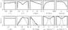 |
Fig. 3 Trends in cluster detectability as a function of ten cluster parameters for the simulated cluster injection and retrievals in this work. In each subplot, the black line shows the fraction of clusters detected, fdetected, while marginalising over all other parameters. For comparison, the grey line shows the distribution of injected clusters in this work, normalised to have a maximum at one. The top row of plots and the first on the lower row show intrinsic parameters, which are those chosen during this study; the remaining parameters rt, AV, μα*, and μδ are all a function of these intrinsic parameters, but are nevertheless shown here for illustrative purposes. Figure A.1 shows the covariances between the most significant of these parameters. |
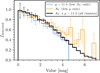 |
Fig. 4 Comparison between the impact of extinction AV and distance modulus μ on cluster detectability, for clusters with a mass below 800 M . The blue curve shows fdetected as a function of distance modulus μ for simulated clusters with negligible extinction (AV < 0.5), while the orange curve shows fdetected as a function of AV for the nearest clusters in this study (2 < d [kpc] < 3). A correction of 11.5 (the distance modulus corresponding to a distance of 2 kpc) was subtracted from the distance modulus to make its value in this study start at zero, and hence be easily comparable with AV, which also has a minimum value of zero in this work. The black curve shows fdetected for μ and AV summed for all simulated clusters. Poisson uncertainties are shown on the bins. |
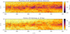 |
Fig. 5 Fraction of simulated clusters recovered compared to the input dust distribution in this study. Top: fraction of all simulated clusters recovered in this work as a function of l and b. Clusters were binned in bins of size 1° × 1°. Grey circles show the distribution of high-quality OCs in HR24 with CST > 5, d > 3 kpc, and a CMD class of better than 0.5. Bottom: as above, but instead showing the total Green et al. (2019) extinction in the V band at a distance of 10 kpc overlaid with real OCs. |
4.2 Interpolating between simulated clusters on our unstructured grid of injection and retrievals
Our cluster injection and retrievals densely sample the parameter space defined in Table 2, allowing for an in-depth study of the cluster selection function towards the Galactic anticentre. However, it is difficult to use an unstructured probabilistic grid of detections to predict the detectability of a single cluster. It is possible to bin the unstructured grid to see broad overviews of detectability, such as binning in l, b, and d and then ‘marginalising’ over all other parameters to see detectability in 3D space; but it is also desirable to have a smooth selection function that allows for predictions at an exact set of cluster parameters. We explored a number of ways to interpolate between grid points on our unstructured grid of detections and construct a smooth selection function for other purposes in this study.
We initially explored the use of radial basis function and nearest neighbour interpolators. However, all interpolation schemes we tried were outperformed by supervised machine learning, with approaches based on the gradient-boosting decision tree algorithm XGBoost6 (Chen & Guestrin 2016) outperforming the best interpolation scheme we trialed in terms of accuracy by a factor of 2.5.
We trained multiple XGBoost predictors, tasked either with regression to predict CST values, or with classification to predict the probability that a cluster has a CST greater than some threshold. This effectively predicts the fraction of clusters with certain parameters detected at a given threshold, and can be written fdetected,CST>x for some threshold x. For CST > 3, this recovers the selection function of HR23, who used such a threshold to clean their catalogue of poor-quality detections; higher thresholds are also useful to study the selection function of more astrometrically reliable clusters.
We first trained our models on nine parameters: (l, b, d, M, log t, rc, rt, μα*, and μδ). However, since we found that rc and rt had a negligible effect on cluster detectability (see Fig. C.1, and Sect. 4.1 for further discussion), our final models do not incorporate them, and instead only require seven input parameters. For all trained XGBoost models, we used 160 000 simulated clusters for training and kept the remaining 34 752 clusters to use as a validation set. Our final models used 200 estimators, a maximum tree depth of seven, and used a learning rate (eta) of 0.2. Our CST predictor achieved final training and validation data root mean squared errors of 2.77 and 3.17 respectively (meaning that the typical errors of the predictor were around 2.77 and 3.17 respectively), with our fdetected predictors achieving a typical binary classification accuracy on training and validation data of 94% and 91% respectively. Higher accuracies than this were not possible to achieve even with careful parameter tuning. Some of these residuals are due to sharp local variations in extinction and field density that XGBoost is not able to fully capture.
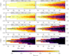 |
Fig. 6 Fraction of simulated clusters recovered as a function of RGC and Z divided into multiple different mass and ages ranges, and compared against the distribution of OCs in HR24 within those ranges. Each row shows clusters in a different mass range, indicated by the label on each subplot. The subplots in the left column show young clusters with log t < 8.5, while subplots in the right column show old clusters with log t > 8.5. Although proper motions only have a small impact on cluster detectability, we nevertheless only show the detection results of simulated clusters with proper motions |μα*| < 2.5 and |μδ| < 2.5, providing a slightly more conservative estimate on cluster detectability at these locations. |
4.3 Validating our results on real clusters
We can now compare the CST predicted by our model to the values obtained by HR24 for clusters of similar parameters, providing an additional test on the reliability of our results. Figure 7 shows the distribution of cluster CSTs as a function of mass for a sample of young and moderately reddened anticentre clusters. The distribution of simulated cluster CSTs closely follows that of OCs in HR24, suggesting that our results are realistic.
For a more complete comparison, we used our CST predictor from Sect. 4.2 to predict the CST of all real clusters in the anticentre. We found that our CST predictor - trained only on our simulated cluster retrieval experiments - had a root mean squared error of 3.75 when tasked with predicting the CST of real OCs in HR24. This is comparable to the root mean squared error of 3.17 that the CST predictor achieved on its simulated validation data, despite the fact that real OCs in HR24 have uncertain parameters.
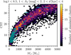 |
Fig. 7 Comparison between the CST of simulated and real clusters in a restricted parameter range as a function of cluster mass. Simulated clusters are shown by the heatmap in the background, while clusters in HR23 are shown by the blue points, plotted as a function of their mass and associated uncertainty from HR24. We use the Jacobi mass MJ from HR24, which measures the mass of the bound part of an OC, as MJ is the most comparable cluster mass to the simulated cluster masses in this study. Only clusters with log t < 8.5, 1 < AV < 2, and 2 < d < 4 kpc are shown. |
5 Answering questions about Galactic structure with our anticentre OC selection function
In this section, we discuss the implications of the OC selection function on our understanding of the outer Galactic disk structure, traced through its cluster population. We comment on the different radial extent of the old and young OCs, on the warp of the disk, and on the potential future discovery of old clusters at very large Galactocentric distances.
5.1 The limiting radius of the OC population as a function of age
The OC selection function we construct in this study indicates that at any given mass, beyond log t~8.5, the detection probability quickly decreases with age. High proper motions and Galactic latitudes do not sufficiently increase detectability to balance the effect of old age.
To quantify the effect of the selection function on an assumed cluster distribution, we generated two cluster populations, corresponding to two different heating regimes. The first one, which we refer to as the kinematically ‘warm’ cluster population, follows a flared vertical density profile with a scale height increasing as t1.3 (Cantat-Gaudin et al. 2020), and an agevelocity relation following Tarricq et al. (2021) which we add to the Milky Way rotation curve of the MWPotential2014 potential of Bovy (2015). The kinematically ‘hot’ population scale height increases with t2, and its velocity dispersion increases three times faster than in Tarricq et al. (2021). The warm population is intended to represent a Milky-Way-like galaxy. The hot population is not meant as a physically plausible model of the Galactic disk, but as an illustration of the effect of extreme dynamical heating on cluster detectability. We convert their intrinsic properties to observable quantities (sky co-ordinates, proper motions) and apply the OC selection function to compute the fraction of recovered objects as a function of Galactocentric radius.
Using our realistic ‘warm’ model of OC kinematics in the Milky Way, Fig. 8 shows the selection-effect corrected fraction of clusters younger than logt = 8.5 as a function of galactocen-tric radius (flog t<8.5). To create this figure, we binned clusters in HR24 with masses between 250 and 2000 M into seven logarithmically spaced mass bins, three bins in distance, and two bins in age (‘young’ and ‘old’), and derived a distance, age, and mass-dependent correction for the count in each bin, averaged across the full anticentre region we consider. This correction was then used to scale the observed count of clusters in each bin to an estimated true count, based on the predicted detectability of 106 clusters across this mass and distance range drawn from our ‘warm’ kinematic model, before finally summing estimated true counts in all mass bins to derive the distribution as a function of age. An additional data point for the solar neighbourhood estimated using the volume-limited complete sample in HR24 is also shown. This result confirms that the observed higher fraction of old clusters in the anticentre is not a selection effect, but rather an intrinsic property of the Milky Way: we find that flog t<8.5 is 2.97 ± 0.11 times lower at RGC = 13 kpc compared to in the solar neighbourhood, dropping from 81.7% ± 9.2% in the solar neighbourhood to 27.5% ± 5.7% in this most distant bin.
Curiously, our selection effect-corrected flog t<8.5 remains relatively similar to the observed distribution of this quantity in HR24 - at least within our considered distance and mass ranges.
Only the highest distance bin in Fig. 8 appears significantly different to the observed distribution (i.e. the grey line), likely because it corresponds to the distance range in which old clusters start to become significantly more challenging to recover compared to young clusters (Fig. 6). Cluster mass appears to remain the most significant parameter impacting cluster detectability, and not age (see also Appendix C), causing the simple ratio between young and old clusters within some distant range to not be strongly biased by detection effects due to age. Estimating flog t<8.5 at distances greater than 14 kpc is not possible with our simple binning-based approach due to the small number statistics of young clusters at this distance; a forward modelling-based approach should be explored in the future using our selection function to allow for a smooth model to be fit to flog t<8.5.
Figure 8 also shows that the greater scale height and hotter orbits of old clusters are not significant enough to explain their higher fraction in the anticentre. To further illustrate the implausibility of flog t<8.5 being flat as a function of RGC, Fig. 9 shows the impact of assuming our unrealistically ‘hot’ kinematics on the detectability of OCs for three chosen masses (200, 800, and 2000 M). While the hot cluster population allows for a higher detection fraction at a given age than the warm population, its extreme combination of large scale heights and hot proper motions is never sufficient to make old clusters significantly more detectable than younger ones. Based on our current work, it seems unlikely that the larger relative number of known old clusters in the outer Milky Way (Fig. 1) is caused by an observational bias favouring old clusters, with it instead being more likely that young clusters are either scarcer than old clusters or have lower masses. Other age-dependent effects could be investigated in the future (such as mass segregation or alternative cluster models to a King model), although they would have to make up for a large difference in cluster detectability as a function of age to counter the result in this work.
The diminishing number of young clusters with increasing Galactocentric radius is however not an indication of a lack of star formation, as young field stars are visible as far as 18 kpc from the Galactic centre (e.g. Cepheids, Lemasle et al. 2022). We therefore argue that RGC ~ 13 kpc could be the limit for massive cluster formation, rather than the absolute cut-off radius of star formation in the Milky Way. While our experiment confidently establishes that old massive clusters are more numerous than young massive clusters in the outer disc, it also demonstrates that the Gaia-DR3-based cluster census is highly incomplete for distant low-mass clusters of all ages (bottom panels of Fig. 6; top left panel of Fig. 9).
Rather than a constraint on the total number of young low-mass clusters, our results could be interpreted as an upper limit on the mass of clusters forming in the outer Milky Way. This interpretation supports the theory proposed by Pflamm-Altenburg & Kroupa (2008) to explain why the radial density profiles of external galaxies exhibit a sharp edge in Ha, but a much smoother UV (ultraviolet) profile. The authors propose that lower gas densities reduce the maximum mass that clusters can form at. In this scenario, the massive old clusters currently found in the outer-disc formed in the inner Milky Way before migrating outwards, where weaker tidal forces (Lamers et al. 2005) and the larger vertical excursion (Viscasillas Vázquez et al. 2023; Moreira et al. 2025) increased the timescale for their disruption.
Migration would also be responsible for the flattening of the radial metallicity gradient, whose change of slope occurs near RGC ~ 12kpc (Donor et al. 2020; Zhang et al. 2021; Myers et al. 2022; Spina et al. 2022; Magrini et al. 2023; Carbajo-Hijarrubia et al. 2024). Studying migration mechanisms in the Milky Way through the lens of OC distributions is complex, as mild perturbations to their orbits may enhance their chances of survival, but strong perturbations can accelerate their disruption. Recent studies estimate the migration rates of OCs around 1 kpc Gyr−1 (Chen & Zhao 2020; Netopil et al. 2022). Chen & Zhao (2020) remark that the metallicities and kinematics of old outer-disc clusters suggest higher migration rates of 1.5±0.5 kpcGyr−1, further supporting the idea that clusters undergoing significant outward migration are more likely to remain bound for billions of years.
However, caution should be taken when dealing with the small sample size of young, massive clusters in the anticentre due to the rarity of young, massive clusters (Lada & Lada 2003; Portegies Zwart et al. 2010). Our result mirrors discussions in extragalactic star cluster samples: while some works find a galactocentric-radius dependent limiting mass for clusters (e.g. Pflamm-Altenburg et al. 2013), other works have demonstrated that a small sample size can cause the appearance of a truncated upper mass limit for clusters (Sun et al. 2016). In general, robustly determining the upper mass limit of cluster censuses is challenging (Krumholz et al. 2019). While we are able to conclude in this work that the anticentre contains more old clusters than young ones, further research will be required to determine the exact reason for this. Alternative hypotheses to cluster migration should be explored, such as a lower cluster disruption rate in the anticentre causing an ‘old-heavy’ cluster age function relative to the solar neighbourhood.
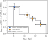 |
Fig. 8 Fraction of OCs that are younger than log t = 8.5 as a function of galactocentric radius, shown only for clusters with masses between 250 and 2000 M . Orange squares show this fraction estimated from cluster counts in HR24 and corrected for incompleteness assuming a ‘warm’ kinematic heating model (Sect. 5.1). The blue square is estimated for clusters within 1 kpc of the Sun in HR24, given that this volume is expected to be ≈100% complete within this mass range (see HR24 Sect. 5.1). The grey line shows this fraction for HR24 clusters in our studied region (140° < l < 240°, |b| < 10°), uncorrected for selection effects. |
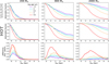 |
Fig. 9 Top: fraction of detectable clusters as a function of Galactocentric radius at three different masses and five different ages, for the simulated kinematically warm cluster population (see text). Middle: same as above, for the kinematically hot cluster population. Bottom: difference between hot and warm detectability fractions. |
5.2 The influence of the Galactic warp on the distribution of clusters
The Milky Way features a warped distribution of neutral hydrogen gas in the anticentre (Kalberla et al. 2007; Levine et al. 2006), which has also been shown with the distribution of Cepheid variable stars (e.g. Feast et al. 2014; Skowron et al. 2019; Chen et al. 2019; Lemasle et al. 2022), young OCs (e.g. Moitinho et al. 2006; Vázquez et al. 2008), old OCs (e.g. Cantat-Gaudin et al. 2020; He 2023), and red clump stars (e.g. Momany et al. 2006). The warp is also visible in the old cluster distribution in Fig. 1. In HR24 and using ages from Cavallo et al. (2024), restricting analysis to old (log t > 8.8) OCs with 12 < RGC [kpc] < 16, and using a slightly higher CST cut to improve cluster reliability (CST > 4σ), there are just six clusters above the disk (500 > Z [pc] > 2000) compared to 21 below the disk (−500 < Z [pc] < −2000). This difference in cluster counts can be interpreted as being due to the Galactic warp; however, if a selection bias towards the anticentre existed that made clusters, stars, and gas harder to detect above the disk than below the disk, flaring of the disk with an obscured upper part would present as an asymmetric warp.
As a simple test of the selection dependence of the observed warped cluster distribution, we tested whether it is easier to detect the population of below-disk clusters below or above the disk. To do so, we calculated the probability of detecting the below-disk population of clusters at CST > 4σ below and above the disk by taking the 21 below disk clusters and simply flipping the sign of their Z co-ordinate, and then calculating the mean fdetected,CST>4 value of these clusters with our model from Sect. 4.2, in addition to comparing this to their fdetected,CST>4 below the disk. The mean detection probability of the below disk clusters is 0.40, suggesting that most of the below-disk cluster population in HR24 was somewhat difficult to detect; on the other hand, it would be nearly twice as easy to see the below-disk cluster population above the disk, as the mean detection probability of the below-disk clusters if they were instead above the disk would be 0.74. This difference is likely due to the generally higher extinction below the disk than above it in the direction of the Galactic anticentre (see lower panel of Fig. 5).
Correcting for selection effects, we would expect to see 52.5 ± 11.4 clusters below the disk and 8.1 ± 3.3 clusters above the disk with similar parameters to the 21 below the disk in HR24. Adding the uncertainties on these quantities together in quadrature, we find a statistical difference between these counts at the 3.7σ level, which is strong evidence that the warp in the OC census is nota selection effect. In fact, if all clusters were visible, then the warp in the OC census would present itself nearly twice as strongly as it currently does in the old OC distribution.
5.3 The isolation of Saurer 1 and Berkeley 29
Our cluster selection function also allows for the study of OCs at a more individual level. Arguably the most puzzling objects in the Galactic anticentre are Berkeley 29 and Saurer 1, two old (log t > 9.5) OCs at a significantly larger RGC than any other known OC (see Fig. 1). These objects are just about visible in Gaia DR3 (Gaia Collaboration 2021a; Perren et al. 2022), although only Berkeley 29 appears in HR23 and HR24 and with a modest CST of 5.99. In Gaia Collaboration (2021a), it appears that Saurer 1 has fewer stars than Berkeley 29, suggesting that it is smaller and thus harder to detect due to its lower mass.
Figure 6 shows that the detection of Berkeley 29 by HR23 may be somewhat lucky and depend on its position in the galaxy. Old clusters are almost impossible to detect at low Z values at the distance of Berkeley 29, particularly if their mass is below 1000 M⊙. Its location at a high b of 7.98° above the dusty plane of the Milky Way may be the only reason why it is visible. Between where the main OC distribution truncates at RGC ~ 14 to 15 kpc and the 19 kpc distance of Berkeley 29, it is easy to imagine that many old clusters could hide in the dust-obscured void in Fig. 6 at low |Z|. In the solar neighbourhood, old clusters with masses of just a few hundred solar masses are not especially rare (such as the Hyades or Ruprecht 147), with low-mass old clusters in fact being more common than high-mass ones (HR24, Fig. 15); a similar mass distribution in the anticentre would imply dozens of low-mass or low-|Z| clusters are waiting to be discovered.
The detection of Berkeley 29 may also be dependent on its location in Galactic longitude along the disk. Figure 10 shows the detectability of old and relatively high-mass clusters with parameters similar to Berkeley 29. As with the Galactic warp in Sect. 5.2, it is around twice as easy to detect Berkeley 29 above the disk than below it, largely due to extinction - suggesting that Berkeley 29 could have many low-Z counterparts. In addition, the left side of the anticentre (l > 180°) appears to be the easiest place to see distant old clusters in, with the upper-right of the anticentre being significantly more difficult than the upper-left. In 3D, it appears that Saurer 1 and Berkeley 29 are in the easiest part of the distant anticentre to detect clusters, and we hypothesise that deeper astrometric and photometric surveys of the anticentre such as Gaia DR4 or the proposed GaiaNIR mission (Hobbs & H0g 2018) will find additional clusters in this region. The southern hemisphere location of the Vera Rubin Observatory is better suited to observe the Galactic centre, but LSST may provide enough deep astrometric and photometric data in the medium term of some anticentre regions to allow for the discovery of more anticentre clusters (Ivezić et al. 2019; Usher et al. 2023), particularly when using co-added images that could reach up to six magnitudes deeper than Gaia’s G ≈ 20.7 magnitude limit.
No other OCs as distant as these are known in the Galactic anticentre, which poses the question of whether Berkeley 29 and Saurer 1 are exceptions to the OC distribution, or whether there is a population of distant and old relic OCs in the anticentre yet to be discovered due to selection effects. Improving our knowledge of the old residents of the outer-disc would help us put better constraints on the efficiency of the mechanisms driving stellar migration, and their role in preserving bound clusters. Once believed to be of extragalactic origin, all currently known old distant clusters (including Berkeley 29 and Saurer 1) have been shown beyond reasonable doubt to have formed inside the Milky Way (e.g. Carraro et al. 2007; Cantat-Gaudin et al. 2016; Gaia Collaboration 2021a). The present study also shows that these two clusters, once thought to be ‘alien’, might very well be the tip of the iceberg of a population of distant outer galaxy clusters that are as yet undiscovered.
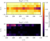 |
Fig. 10 Fraction of simulated clusters recovered at young and old ages compared to the location of old distant clusters Berkeley 29 and Saurer 1. Top: sky distribution of simulated cluster recoveries for young clusters log t < 7.5, at distances greater than 10 kpc, and with masses in the range 1500 < M < 2500 M⊙. Bottom: as above, but for old clusters with log t > 9.5. The location of Berkeley 29 is indicated by a white circle; the location of Saurer 1 is indicated by a white cross. |
6 Conclusions and future outlook
In this paper, we demonstrated injection and retrieval of simulated clusters as a way to determine an empirical star cluster selection function for the Milky Way, beginning with the present study focusing on the Galactic anticentre. We began by generating a large sample of mock clusters spanning a wide range of parameters, and injected them into the Gaia DR3 catalogue in the direction of the Galactic anticentre. We then ran the HDBSCAN-based OC detection strategy of HR23 and attempted to recover the simulated clusters. We built a model of detection probabilities as a function of the main cluster parameters, thus constructing the cluster selection function of the HR24 catalogue in the Galactic anticentre.
We investigated the impact of different cluster parameters, finding that the mass, distance, extinction, and age of a cluster are the most fundamental parameters influencing its detectability. In addition, the proper motion of a cluster can also have a sizeable impact on its detectability, with clusters with the most distinct velocity from that of the field stars around it being easier to detect. We also show that, for Gaia’s broad-band optical observations, distance modulus and extinction have a similar level of impact on cluster detectability. In this work, we do not find that cluster detectability depends critically on the radial profile of a cluster, although this should be investigated further in future works, including exploring the impact of effects such as mass segregation.
Using our cluster selection function, we show that old clusters are significantly harder to recover than young clusters in the outer Galaxy, despite catalogues containing a larger number of old clusters in the outer-disc. We conducted forward-modelling of the cluster incompleteness and find that clusters older than log t = 8.5 are 2.97 ± 0.11 times more common at a Galactocen-tric radius of 13 kpc than in the solar neighbourhood - despite other positive detection biases in their favour, such as hotter orbits or a higher scale height. We conclude from this experiment that few young clusters remain to be found at large Galactocen-tric distances, while the old cluster census is potentially very incomplete. In particular, we show that the most distant known clusters in the Galactic anticentre - Berkeley 29 and Saurer 1 -are likely to have been detected because of their favourably high Galactic latitude away from the dusty plane of the Milky Way. We expect that these two clusters may be the tip of the iceberg of a population of distant, old clusters in the Galactic anticentre. We interpret the presence of a population of old massive clusters in the distant outer regions of the Milky Way as a combination of efficient migration mechanisms and a longer cluster survival time in the outer-disc.
Our work is not without some caveats that future studies should address. Firstly, our work implicitly assumes that object classifications in HR24 are correct. Principally, this requires that cluster masses and radii in HR24 are correct enough to avoid misclassifying bound clusters as unbound ones. While this has a small impact on our studied distant region in the anticentre (Table 1), this will need to be addressed further when extending our methodology to regions of HR24 that contain a higher number of moving groups. Secondly, our work does not establish the selection function of the HR23 CMD classifier, and hence cannot yet be used to determine the selection function of their high-quality cluster sample. Finally, since our selection function depends strongly on a number of observables that are difficult to calculate accurately for clusters (such as mass, age, or extinction), the applicability of our selection function is also somewhat limited by the quality of cluster parameters. Efforts should be made to continue improving cluster parameter determination in the future, particularly by using upcoming data releases from Gaia and other surveys. In addition, better quantifying the systematics of these parameter determinations would allow for corrections for wrongly assigned parameters to be incorporated into future cluster selection functions.
The methodology we developed for this study can be applied to the entire Gaia catalogue. In a future work, we will address the computational challenges involved in applying our method across the whole Gaia catalogue, and we will release an opensource selection function of the HR24 OC catalogue. A key application of this selection function will be in constructing a full model of the currently unknown age-mass distribution of OCs across the full Milky Way, allowing for OCs to trace cluster formation and destruction rates across the full Galactic disk. In addition to increasing the utility of OCs in mapping Galactic structure, our cluster selection function products and methodology could be used for many other purposes, such as: determining how many stars are missing from a given cluster, calculating the detection probability of OC tidal tails, or estimating how many clusters future surveys or data releases may be able to detect. We plan to explore these possibilities in future works.
Acknowledgements
We thank the anonymous referee for their detailed comments and feedback which greatly improved the clarity of this work. We also thank the organizers of the “From star clusters to field populations: survived, destroyed and migrated clusters” workshop in 2023 in Florence, Italy, which enabled discussions and collaborations that led to this paper. This work has made use of data from the European Space Agency (ESA) mission Gaia (http://www.cosmos.esa.int/gaia), processed by the Gaia Data Processing and Analysis Consortium (DPAC, http://www.cosmos.esa.int/web/gaia/dpac/consortium). Funding for the DPAC has been provided by national institutions, in particular the institutions participating in the Gaia Multilateral Agreement. This work is a result of the GaiaUnlimited project, which has received funding from the European Union’s Horizon 2020 research and innovation programme under grant agreement No 101004110. The GaiaUnlimited project was started at the 2019 Santa Barbara Gaia Sprint, hosted by the Kavli Institute for Theoretical Physics at the University of California, Santa Barbara. This work was (partially) supported by the Spanish MICIN/AEI/10.13039/501100011033 and by “ERDF A way of making Europe” by the European Union through grant PID2021-122842OB-C21, and the Institute of Cosmos Sciences University of Barcelona (ICCUB, Unidad de Excelencia ‘María de Maeztu’) through grant CEX2019-000918-M. F.A. acknowledges the grant RYC2021-031683-I funded by MCIN/AEI/10.13039/501100011033 and by the European Union’s NextGener-ationEU/PRTR. In addition to those listed in the text, this work made use of the following software packages: Jupyter (Perez & Granger 2007; Kluyver et al. 2016), matplotlib (Hunter 2007), numpy (Harris et al. 2020), pandas (McKinney 2010; The Pandas development team 2024), python (Van Rossum & Drake 2009), scipy (Virtanen et al. 2020; Gommers et al. 2024), astroquery (Ginsburg et al. 2019; Ginsburg et al. 2024), Cython (Behnel et al. 2011), Numba (Lam et al. 2015; Lam et al. 2024), and scikit-learn (Pedregosa et al. 2011; Buitinck et al. 2013; Grisel et al. 2024). This research has made use of NASA’s Astrophysics Data System. This research also made use of the SIMBAD database, operated at CDS, Strasbourg, France (Wenger, M. et al. 2000). Software citation information aggregated using The Software Citation Station (Wagg & Broekgaarden 2024; Wagg et al. 2024). This work used the accessible Matplotlib-like colour cycles defined in Petroff (2021).
Appendix A Correlations in detectability between cluster parameters
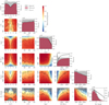 |
Fig. A.1 Cornerplot summarising the covariances between parameters further to those discussed in Sect. 4.1 and shown in Fig. 3. In the diagonal panels, we show the 1D parameter distributions of the simulated and recovered clusters in grey and red respectively. The fraction of detected objects are shown as a solid black line. The off-diagonal panels are heat maps showing the fraction of injected clusters that were recovered as a function of two parameters. We superimpose contours of iso-detectability with dotted, dash-dotted, dashed, and solid lines at fdetected equal to 0.2, 0.4, 0.6, and 0.8, respectively. Grey areas indicate regions of the parameter space where we do not inject OCs. These individual heatmaps can be used to visually find regions where, for instance, almost all clusters are detectable (solid red regions), where almost no clusters are detectable (solid blue regions), or regions where detectability changes sharply as a function of certain parameters, as well as the trend between them. |
Appendix B Injected cluster proper motions
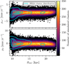 |
Fig. B.1 Comparison between the proper motions of our injected clusters and clusters in HR24 as a function of galactocentric radius. All 192 318 simulated clusters are shown by the heatmap, with a colour bar on the right. The proper motion distribution of the 818 HR24 clusters within our studied region is shown by the kernel density estimate, with contours at the 0.1%, 20%, 50%, and 80% density levels. |
Appendix C Interpreting the machine learning model
To better quantify why certain clusters can or cannot be detected, we applied Shapley Additive Explanations7 (SHAP Lundberg & Lee 2017) to explain the importance of features to our CST prediction model from Sect. 4.2. Figure C.1 shows the SHAP feature importance of different cluster parameters. For the upper panel in Fig. C.1, the width and colour coding of each row of the beeswarm plot shows the impact of different parameters on the CST. Cluster mass, distance, age, and b have the largest impact on cluster significance respectively. The x axis shows the impact of different input features on the CST that the model predicts, and the difference in CST between the upper and lower values in our studied parameter ranges from Table 2 can hence be read directly off of the x axis of the plot. For instance, a cluster with a mass of 50 M will have a CST 30σ lower than a cluster with a mass of 5000 M.
The SHAP interpretation also allows for the study of more subtle parameter effects. Although proper motion has a smaller impact than other parameters on the detectability of a cluster, trends in how it impacts CST are still visible. The bottom panel of Fig. C.1 shows how the CST of the model changes as a function of μδ and at given Galactic longitude values. The impact of cluster proper motion on CST is a ‘V’ shape, with values of proper motion distinct from that of the field causing cluster detectability to increase. As l increases, the typical proper motion of the field also increases slightly, causing the ‘V’ shape to traverse to higher μδ values. In general, proper motion at the distance range studied in this work causes CST to increase by around 3σ for every 4 mas yr−1 that the cluster’s μδ is different from that of the field. A CST change of 3σ could still be the difference between a cluster being detected and included in HR23 or not. This also shows that studies of the velocity distribution of OCs based on Gaia data will be biased towards including clusters with more extreme orbits unless they also account for selection effects.
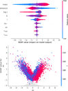 |
Fig. C.1 SHAP feature importance values for the CST predictor. Top: Beeswarm plot where each cluster in the validation dataset is shown as a dot. Each row corresponds to the impact of a different input parameter. The colour coding corresponds to whether it was a high or low value of the parameter. The x axis shows the final impact on the output of the model, which is how much the CST is changed for that given cluster and that given parameter value. For example: for cluster mass, low mass values (blue) correspond to a much lower SHAP/CST, whereas high mass values (red) correspond to a much higher SHAP/CST. On the other hand, most age values have minimal impact on CST, although high ages significantly reduce it. Bottom: SHAP value at a given pmdec as a function of pmdec and shown for all clusters in the validation dataset. Colour coding shows the Galactic longitude, l. |
References
- Alessi, B. S., Moitinho, A., & Dias, W. S. 2003, A&A, 410, 565 [NASA ADS] [CrossRef] [EDP Sciences] [Google Scholar]
- Almeida, A., Monteiro, H., & Dias, W. S. 2023, MNRAS, 525, 2315 [NASA ADS] [CrossRef] [Google Scholar]
- Almeida, D., Moitinho, A., & Moreira, S. 2025, A&A, 693, A305 [NASA ADS] [CrossRef] [EDP Sciences] [Google Scholar]
- Anders, F., Cantat-Gaudin, T., Quadrino-Lodoso, I., et al. 2021, A&A, 645, L2 [NASA ADS] [CrossRef] [EDP Sciences] [Google Scholar]
- Astropy Collaboration (Robitaille, T. P., et al.) 2013, A&A, 558, A33 [NASA ADS] [CrossRef] [EDP Sciences] [Google Scholar]
- Astropy Collaboration (Price-Whelan, A. M., et al.) 2018, AJ, 156, 123 [Google Scholar]
- Astropy Collaboration (Price-Whelan, A. M., et al.) 2022, ApJ, 935, 167 [NASA ADS] [CrossRef] [Google Scholar]
- Behnel, S., Bradshaw, R., Citro, C., et al. 2011, Comput. Sci. Eng., 13, 31 [Google Scholar]
- Bovy, J. 2015, ApJS, 216, 29 [NASA ADS] [CrossRef] [Google Scholar]
- Bressan, A., Marigo, P., Girardi, L., et al. 2012, MNRAS, 427, 127 [NASA ADS] [CrossRef] [Google Scholar]
- Brown, A. G. A. 2021, ARA&A, 59, 59 [NASA ADS] [CrossRef] [Google Scholar]
- Buitinck, L., Louppe, G., Blondel, M., et al. 2013, in ECML PKDD Workshop: Languages for Data Mining and Machine Learning, 108 [Google Scholar]
- Campello, R. J. G. B., Moulavi, D., & Sander, J. 2013, in Advances in Knowledge Discovery and Data Mining, eds. J. Pei, V. S. Tseng, L. Cao, H. Motoda, & G. Xu (Berlin, Heidelberg: Springer), 160 [Google Scholar]
- Cantat-Gaudin, T. 2022, Universe, 8, 111 [NASA ADS] [CrossRef] [Google Scholar]
- Cantat-Gaudin, T., & Anders, F. 2020, A&A, 633, A99 [NASA ADS] [CrossRef] [EDP Sciences] [Google Scholar]
- Cantat-Gaudin, T., Donati, P., Vallenari, A., et al. 2016, A&A, 588, A120 [NASA ADS] [CrossRef] [EDP Sciences] [Google Scholar]
- Cantat-Gaudin, T., Jordi, C., Vallenari, A., et al. 2018, A&A, 618, A93 [NASA ADS] [CrossRef] [EDP Sciences] [Google Scholar]
- Cantat-Gaudin, T., Krone-Martins, A., Sedaghat, N., et al. 2019, A&A, 624, A126 [NASA ADS] [CrossRef] [EDP Sciences] [Google Scholar]
- Cantat-Gaudin, T., Anders, F., Castro-Ginard, A., et al. 2020, A&A, 640, A1 [NASA ADS] [CrossRef] [EDP Sciences] [Google Scholar]
- Cantat-Gaudin, T., Fouesneau, M., Rix, H.-W., et al. 2023, A&A, 669, A55 [NASA ADS] [CrossRef] [EDP Sciences] [Google Scholar]
- Carbajo-Hijarrubia, J., Casamiquela, L., Carrera, R., et al. 2024, A&A, 687, A239 [NASA ADS] [CrossRef] [EDP Sciences] [Google Scholar]
- Carraro, G., Geisler, D., Villanova, S., Frinchaboy, P. M., & Majewski, S. R. 2007, A&A, 476, 217 [NASA ADS] [CrossRef] [EDP Sciences] [Google Scholar]
- Castro-Ginard, A., Jordi, C., Luri, X., et al. 2018, A&A, 618, A59 [NASA ADS] [CrossRef] [EDP Sciences] [Google Scholar]
- Castro-Ginard, A., Jordi, C., Luri, X., et al. 2020, A&A, 635, A45 [NASA ADS] [CrossRef] [EDP Sciences] [Google Scholar]
- Castro-Ginard, A., Brown, A. G. A., Kostrzewa-Rutkowska, Z., et al. 2023, A&A, 677, A37 [NASA ADS] [CrossRef] [EDP Sciences] [Google Scholar]
- Cavallo, L., Spina, L., Carraro, G., et al. 2024, AJ, 167, 12 [NASA ADS] [CrossRef] [Google Scholar]
- Chen, T., & Guestrin, C. 2016, in Proceedings of the 22nd ACM SIGKDD International Conference on Knowledge Discovery and Data Mining, KDD ’16 (New York, NY, USA: ACM), 785 [Google Scholar]
- Chen, Y. Q., & Zhao, G. 2020, MNRAS, 495, 2673 [NASA ADS] [CrossRef] [Google Scholar]
- Chen, Y., Girardi, L., Bressan, A., et al. 2014, MNRAS, 444, 2525 [Google Scholar]
- Chen, Y., Bressan, A., Girardi, L., et al. 2015, MNRAS, 452, 1068 [Google Scholar]
- Chen, X., Wang, S., Deng, L., et al. 2019, Nat. Astron., 3, 320 [NASA ADS] [CrossRef] [Google Scholar]
- Dias, W. S., Alessi, B. S., Moitinho, A., & Lépine, J. R. D. 2002, A&A, 389, 871 [NASA ADS] [CrossRef] [EDP Sciences] [Google Scholar]
- Donor, J., Frinchaboy, P. M., Cunha, K., et al. 2020, AJ, 159, 199 [NASA ADS] [CrossRef] [Google Scholar]
- Fabricius, C., Luri, X., Arenou, F., et al. 2021, A&A, 649, A5 [NASA ADS] [CrossRef] [EDP Sciences] [Google Scholar]
- Feast, M. W., Menzies, J. W., Matsunaga, N., & Whitelock, P. A. 2014, Nature, 509, 342 [Google Scholar]
- Froebrich, D., Scholz, A., & Raftery, C. L. 2007, MNRAS, 374, 399 [Google Scholar]
- Gaia Collaboration (Prusti, T., et al.) 2016, A&A, 595, A1 [NASA ADS] [CrossRef] [EDP Sciences] [Google Scholar]
- Gaia Collaboration (Brown, A. G. A., et al.) 2018, A&A, 616, A1 [NASA ADS] [CrossRef] [EDP Sciences] [Google Scholar]
- Gaia Collaboration (Antoja, T., et al.) 2021a, A&A, 649, A8 [EDP Sciences] [Google Scholar]
- Gaia Collaboration (Brown, A. G. A., et al.) 2021b, A&A, 649, A1 [NASA ADS] [CrossRef] [EDP Sciences] [Google Scholar]
- Ginsburg, A., Sipőcz, B. M., Brasseur, C. E., et al. 2019, AJ, 157, 98 [Google Scholar]
- Ginsburg, A., Sipőcz, B., Brasseur, C. E., et al. 2024, https://doi.org/10.5281/zenodo.10799414 [Google Scholar]
- Gommers, R., Virtanen, P., Haberland, M., et al. 2024, https://doi.org/10.5281/zenodo.10909890 [Google Scholar]
- Górski, K. M., Hivon, E., Banday, A. J., et al. 2005, ApJ, 622, 759 [Google Scholar]
- Green, G. M., Schlafly, E., Zucker, C., Speagle, J. S., & Finkbeiner, D. 2019, ApJ, 887, 93 [NASA ADS] [CrossRef] [Google Scholar]
- Grisel, O., Mueller, A., Lars, et al. 2024, https://doi.org/10.5281/zenodo.10951361 [Google Scholar]
- Harris, C. R., Millman, K. J., van der Walt, S. J., et al. 2020, Nature, 585, 357 [NASA ADS] [CrossRef] [Google Scholar]
- He, Z. 2023, ApJ, 954, L9 [Google Scholar]
- Herschel, W. 1786, Phil. Trans. R. Soc. London Ser. I, 76, 457 [Google Scholar]
- Herschel, W. 1789, Phil. Trans. R. Soc. London Ser. I, 79, 212 [Google Scholar]
- Hobbs, D., & Hog, E. 2018, IAU Symp., 330, 67 [Google Scholar]
- Hunt, E. L., & Reffert, S. 2021, A&A, 646, A104 [NASA ADS] [CrossRef] [EDP Sciences] [Google Scholar]
- Hunt, E. L., & Reffert, S. 2023, A&A, 673, A114 [NASA ADS] [CrossRef] [EDP Sciences] [Google Scholar]
- Hunt, E. L., & Reffert, S. 2024, A&A, 686, A42 [NASA ADS] [CrossRef] [EDP Sciences] [Google Scholar]
- Hunter, J. D. 2007, Comput. Sci. Eng., 9, 90 [NASA ADS] [CrossRef] [Google Scholar]
- Ivezić, Ž., Kahn, S. M., Tyson, J. A., et al. 2019, ApJ, 873, 111 [Google Scholar]
- Janes, K., & Adler, D. 1982, ApJS, 49, 425 [Google Scholar]
- Kalberla, P. M. W., Dedes, L., Kerp, J., & Haud, U. 2007, A&A, 469, 511 [NASA ADS] [CrossRef] [EDP Sciences] [Google Scholar]
- Kharchenko, N. V., Piskunov, A. E., Röser, S., Schilbach, E., & Scholz, R. D. 2005, A&A, 440, 403 [NASA ADS] [CrossRef] [EDP Sciences] [Google Scholar]
- Kharchenko, N. V., Piskunov, A. E., Schilbach, E., Röser, S., & Scholz, R. D. 2013, A&A, 558, A53 [NASA ADS] [CrossRef] [EDP Sciences] [Google Scholar]
- King, I. 1962, AJ, 67, 471 [Google Scholar]
- Kluyver, T., Ragan-Kelley, B., Pérez, F., et al. 2016, in ELPUB, 87 [Google Scholar]
- Koposov, S., Belokurov, V., Evans, N. W., et al. 2008, ApJ, 686, 279 [NASA ADS] [CrossRef] [Google Scholar]
- Kroupa, P. 2001, MNRAS, 322, 231 [NASA ADS] [CrossRef] [Google Scholar]
- Krumholz, M. R., McKee, C. F., & Bland-Hawthorn, J. 2019, ARA&A, 57, 227 [NASA ADS] [CrossRef] [Google Scholar]
- Lada, C. J., & Lada, E. A. 2003, ARA&A, 41, 57 [Google Scholar]
- Lam, S. K., Pitrou, A., & Seibert, S. 2015, in Proc. Second Workshop on the LLVM Compiler Infrastructure in HPC, 1 [Google Scholar]
- Lam, S. K., stuartarchibald, Pitrou, A., et al. 2024, https://doi.org/10.5281/zenodo.10839385 [Google Scholar]
- Lamers, H. J. G. L. M., Gieles, M., Bastian, N., et al. 2005, A&A, 441, 117 [NASA ADS] [CrossRef] [EDP Sciences] [Google Scholar]
- Lemasle, B., Lala, H. N., Kovtyukh, V., et al. 2022, A&A, 668, A40 [NASA ADS] [CrossRef] [EDP Sciences] [Google Scholar]
- Levine, E. S., Blitz, L., & Heiles, C. 2006, ApJ, 643, 881 [NASA ADS] [CrossRef] [Google Scholar]
- Lindegren, L., & Dravins, D. 2021, A&A, 652, A45 [NASA ADS] [CrossRef] [EDP Sciences] [Google Scholar]
- Lindegren, L., Klioner, S. A., Hernández, J., et al. 2021, A&A, 649, A2 [EDP Sciences] [Google Scholar]
- Lundberg, S. M., & Lee, S.-I. 2017, in Advances in Neural Information Processing Systems 30, eds. I. Guyon, U. V. Luxburg, S. Bengio, et al. (UK: Curran Associates, Inc.), 4765 [Google Scholar]
- Magrini, L., Viscasillas Vázquez, C., Spina, L., et al. 2023, A&A, 669, A119 [NASA ADS] [CrossRef] [EDP Sciences] [Google Scholar]
- McInnes, L., Healy, J., & Astels, S. 2017, J. Open Source Softw., 2, 205 [NASA ADS] [CrossRef] [Google Scholar]
- McKinney, W. 2010, in Proceedings of the 9th Python in Science Conference, eds. S. van der Walt, & J. Millman, 56 [Google Scholar]
- Messier, C. 1781, Catalogue des Nébuleuses et des Amas d’étoiles (Catalog of Nebulae and Star Clusters), Connaissance des Temps ou des Mouvements Célestes, for 1784, 227 [Google Scholar]
- Moe, M., & Di Stefano, R. 2017, ApJS, 230, 15 [Google Scholar]
- Moitinho, A., Vázquez, R. A., Carraro, G., et al. 2006, MNRAS, 368, L77 [NASA ADS] [CrossRef] [Google Scholar]
- Momany, Y., Zaggia, S., Gilmore, G., et al. 2006, A&A, 451, 515 [NASA ADS] [CrossRef] [EDP Sciences] [Google Scholar]
- Moreira, S., Moitinho, A., Silva, A., & Almeida, D. 2025, A&A, 694, A70 [NASA ADS] [CrossRef] [EDP Sciences] [Google Scholar]
- Myers, N., Donor, J., Spoo, T., et al. 2022, AJ, 164, 85 [NASA ADS] [CrossRef] [Google Scholar]
- Netopil, M., Paunzen, E., & Stütz, C. 2012, in Star Clusters in the Era of Large Surveys, Astrophysics and Space Science Proceedings (Berlin: Springer), 29, 53 [Google Scholar]
- Netopil, M., Oralhan, I. A., Çakmak, H., Michel, R., & Karataş, Y. 2022, MNRAS, 509, 421 [Google Scholar]
- Pedregosa, F., Varoquaux, G., Gramfort, A., et al. 2011, J. Mach. Learn. Res., 12, 2825 [Google Scholar]
- Perez, F., & Granger, B. E. 2007, Comput. Sci. Eng., 9, 21 [Google Scholar]
- Perren, G. I., Pera, M. S., Navone, H. D., & Vázquez, R. A. 2022, A&A, 663, A131 [NASA ADS] [CrossRef] [EDP Sciences] [Google Scholar]
- Perren, G. I., Pera, M. S., Navone, H. D., & Vázquez, R. A. 2023, MNRAS, 526, 4107 [NASA ADS] [CrossRef] [Google Scholar]
- Petroff, M. A. 2021, ArXiv e-prints [arXiv:2107.02270] [Google Scholar]
- Pflamm-Altenburg, J., & Kroupa, P. 2008, Nature, 455, 641 [Google Scholar]
- Pflamm-Altenburg, J., González-Lópezlira, R. A., & Kroupa, P. 2013, MNRAS, 435, 2604 [CrossRef] [Google Scholar]
- Portegies Zwart, S. F., McMillan, S. L. W., & Gieles, M. 2010, ARA&A, 48, 431 [NASA ADS] [CrossRef] [Google Scholar]
- Riello, M., De Angeli, F., Evans, D. W., et al. 2021, A&A, 649, A3 [NASA ADS] [CrossRef] [EDP Sciences] [Google Scholar]
- Rix, H.-W., Hogg, D. W., Boubert, D., et al. 2021, AJ, 162, 142 [NASA ADS] [CrossRef] [Google Scholar]
- Rybizki, J., Green, G. M., Rix, H.-W., et al. 2022, MNRAS, 510, 2597 [NASA ADS] [CrossRef] [Google Scholar]
- Skowron, D. M., Skowron, J., Mróz, P., et al. 2019, Science, 365, 478 [Google Scholar]
- Spina, L., Magrini, L., & Cunha, K. 2022, Universe, 8, 87 [NASA ADS] [CrossRef] [Google Scholar]
- Sun, W., de Grijs, R., Fan, Z., & Cameron, E. 2016, ApJ, 816, 9 [Google Scholar]
- Tang, J., Bressan, A., Rosenfield, P., et al. 2014, MNRAS, 445, 4287 [NASA ADS] [CrossRef] [Google Scholar]
- Tarricq, Y., Soubiran, C., Casamiquela, L., et al. 2021, A&A, 647, A19 [NASA ADS] [CrossRef] [EDP Sciences] [Google Scholar]
- The Pandas development team 2024, https://doi.org/10.5281/zenodo.10957263 [Google Scholar]
- Trumpler, R. J. 1930, Lick Observ. Bull., 420, 154 [CrossRef] [Google Scholar]
- Usher, C., Dage, K. C., Girardi, L., et al. 2023, PASP, 135, 074201 [NASA ADS] [CrossRef] [Google Scholar]
- Van Rossum, G., & Drake, F. L. 2009, Python 3 Reference Manual (Scotts Valley, CA: CreateSpace) [Google Scholar]
- Vázquez, R. A., May, J., Carraro, G., et al. 2008, ApJ, 672, 930 [CrossRef] [Google Scholar]
- Virtanen, P., Gommers, R., Oliphant, T. E., et al. 2020, Nat. Methods, 17, 261 [Google Scholar]
- Viscasillas Vázquez, C., Magrini, L., Spina, L., et al. 2023, A&A, 679, A122 [NASA ADS] [CrossRef] [EDP Sciences] [Google Scholar]
- Wagg, T., & Broekgaarden, F. S. 2024, ArXiv e-prints [arXiv:2406.04405] [Google Scholar]
- Wagg, T., Broekgaarden, F., & Gültekin, K. 2024, https://doi.org/10.5281/zenodo.13225824 [Google Scholar]
- Wenger, M., Ochsenbein, F., Egret, D., et al. 2000, Astron. Astrophys. Suppl. Ser., 143, 9 [NASA ADS] [CrossRef] [EDP Sciences] [Google Scholar]
- Zhang, H., Chen, Y., & Zhao, G. 2021, ApJ, 919, 52 [NASA ADS] [CrossRef] [Google Scholar]
We refer the reader to Cantat-Gaudin (2022) and Perren et al. (2023) for in-depth reviews of the Gaia contribution to the cluster census.
All Tables
Number of clusters in our studied region in HR23 and HR24 given multiple possible cuts.
All Figures
|
Fig. 1 Spatial distribution of high-certainty clusters (CST>4) from Hunt & Reffert (2023). Ages are taken from Cavallo et al. (2024) as they are more accurate for old clusters (see Sect. 2 for discussion). Top left: histogram of cluster galactocentric radii divided into young (log t < 8.5, blue) and old (log t > 8.5, red) clusters and with a 200 pc bin width. Bottom left: distribution of the same young and old clusters but in terms of altitude Z and Galactocentric radius RGC, assuming RGC,⊙ = 8.2 kpc. Bottom right: projection of these clusters in heliocentric Galactic co-ordinates, with the Sun located at (X,Y) = (0,0). The dotted lines indicate Galactocentric radii from 10 to 18 kpc. The shaded area is the region investigated in this study (140° ≤ ℓ ≤ 240° starting 2 kpc from the Sun). In both lower panels, the cross indicates the cluster Saurer 1, visible in Gaia data but not recovered in the blind search of Hunt & Reffert (2023). |
| In the text | |
|
Fig. 2 Example result of the injection-recovery procedure for a simulated OC, in the typical projections used in cluster discovery studies. Top row: original simulated cluster (including realistic Gaia DR3-like astrometric errors), shown in position (far left), proper motion (centre left), position versus parallax (centre right), and the colour-magnitude diagram of the cluster (far right). This simulated cluster was then inserted into Gaia data to test the cluster recovery ability of HDBSCAN. Bottom row: same as top row, but for the best recovery from Gaia data of this cluster by HDBSCAN. True members of the cluster that were correctly assigned as members by HDBSCAN are shown as blue circles. Non-member field stars from the Gaia dataset that were incorrectly added to the cluster are shown as purple squares. Finally, member stars that HDBSCAN missed are shown as orange crosses. |
| In the text | |
|
Fig. 3 Trends in cluster detectability as a function of ten cluster parameters for the simulated cluster injection and retrievals in this work. In each subplot, the black line shows the fraction of clusters detected, fdetected, while marginalising over all other parameters. For comparison, the grey line shows the distribution of injected clusters in this work, normalised to have a maximum at one. The top row of plots and the first on the lower row show intrinsic parameters, which are those chosen during this study; the remaining parameters rt, AV, μα*, and μδ are all a function of these intrinsic parameters, but are nevertheless shown here for illustrative purposes. Figure A.1 shows the covariances between the most significant of these parameters. |
| In the text | |
|
Fig. 4 Comparison between the impact of extinction AV and distance modulus μ on cluster detectability, for clusters with a mass below 800 M . The blue curve shows fdetected as a function of distance modulus μ for simulated clusters with negligible extinction (AV < 0.5), while the orange curve shows fdetected as a function of AV for the nearest clusters in this study (2 < d [kpc] < 3). A correction of 11.5 (the distance modulus corresponding to a distance of 2 kpc) was subtracted from the distance modulus to make its value in this study start at zero, and hence be easily comparable with AV, which also has a minimum value of zero in this work. The black curve shows fdetected for μ and AV summed for all simulated clusters. Poisson uncertainties are shown on the bins. |
| In the text | |
|
Fig. 5 Fraction of simulated clusters recovered compared to the input dust distribution in this study. Top: fraction of all simulated clusters recovered in this work as a function of l and b. Clusters were binned in bins of size 1° × 1°. Grey circles show the distribution of high-quality OCs in HR24 with CST > 5, d > 3 kpc, and a CMD class of better than 0.5. Bottom: as above, but instead showing the total Green et al. (2019) extinction in the V band at a distance of 10 kpc overlaid with real OCs. |
| In the text | |
|
Fig. 6 Fraction of simulated clusters recovered as a function of RGC and Z divided into multiple different mass and ages ranges, and compared against the distribution of OCs in HR24 within those ranges. Each row shows clusters in a different mass range, indicated by the label on each subplot. The subplots in the left column show young clusters with log t < 8.5, while subplots in the right column show old clusters with log t > 8.5. Although proper motions only have a small impact on cluster detectability, we nevertheless only show the detection results of simulated clusters with proper motions |μα*| < 2.5 and |μδ| < 2.5, providing a slightly more conservative estimate on cluster detectability at these locations. |
| In the text | |
|
Fig. 7 Comparison between the CST of simulated and real clusters in a restricted parameter range as a function of cluster mass. Simulated clusters are shown by the heatmap in the background, while clusters in HR23 are shown by the blue points, plotted as a function of their mass and associated uncertainty from HR24. We use the Jacobi mass MJ from HR24, which measures the mass of the bound part of an OC, as MJ is the most comparable cluster mass to the simulated cluster masses in this study. Only clusters with log t < 8.5, 1 < AV < 2, and 2 < d < 4 kpc are shown. |
| In the text | |
|
Fig. 8 Fraction of OCs that are younger than log t = 8.5 as a function of galactocentric radius, shown only for clusters with masses between 250 and 2000 M . Orange squares show this fraction estimated from cluster counts in HR24 and corrected for incompleteness assuming a ‘warm’ kinematic heating model (Sect. 5.1). The blue square is estimated for clusters within 1 kpc of the Sun in HR24, given that this volume is expected to be ≈100% complete within this mass range (see HR24 Sect. 5.1). The grey line shows this fraction for HR24 clusters in our studied region (140° < l < 240°, |b| < 10°), uncorrected for selection effects. |
| In the text | |
|
Fig. 9 Top: fraction of detectable clusters as a function of Galactocentric radius at three different masses and five different ages, for the simulated kinematically warm cluster population (see text). Middle: same as above, for the kinematically hot cluster population. Bottom: difference between hot and warm detectability fractions. |
| In the text | |
|
Fig. 10 Fraction of simulated clusters recovered at young and old ages compared to the location of old distant clusters Berkeley 29 and Saurer 1. Top: sky distribution of simulated cluster recoveries for young clusters log t < 7.5, at distances greater than 10 kpc, and with masses in the range 1500 < M < 2500 M⊙. Bottom: as above, but for old clusters with log t > 9.5. The location of Berkeley 29 is indicated by a white circle; the location of Saurer 1 is indicated by a white cross. |
| In the text | |
|
Fig. A.1 Cornerplot summarising the covariances between parameters further to those discussed in Sect. 4.1 and shown in Fig. 3. In the diagonal panels, we show the 1D parameter distributions of the simulated and recovered clusters in grey and red respectively. The fraction of detected objects are shown as a solid black line. The off-diagonal panels are heat maps showing the fraction of injected clusters that were recovered as a function of two parameters. We superimpose contours of iso-detectability with dotted, dash-dotted, dashed, and solid lines at fdetected equal to 0.2, 0.4, 0.6, and 0.8, respectively. Grey areas indicate regions of the parameter space where we do not inject OCs. These individual heatmaps can be used to visually find regions where, for instance, almost all clusters are detectable (solid red regions), where almost no clusters are detectable (solid blue regions), or regions where detectability changes sharply as a function of certain parameters, as well as the trend between them. |
| In the text | |
|
Fig. B.1 Comparison between the proper motions of our injected clusters and clusters in HR24 as a function of galactocentric radius. All 192 318 simulated clusters are shown by the heatmap, with a colour bar on the right. The proper motion distribution of the 818 HR24 clusters within our studied region is shown by the kernel density estimate, with contours at the 0.1%, 20%, 50%, and 80% density levels. |
| In the text | |
|
Fig. C.1 SHAP feature importance values for the CST predictor. Top: Beeswarm plot where each cluster in the validation dataset is shown as a dot. Each row corresponds to the impact of a different input parameter. The colour coding corresponds to whether it was a high or low value of the parameter. The x axis shows the final impact on the output of the model, which is how much the CST is changed for that given cluster and that given parameter value. For example: for cluster mass, low mass values (blue) correspond to a much lower SHAP/CST, whereas high mass values (red) correspond to a much higher SHAP/CST. On the other hand, most age values have minimal impact on CST, although high ages significantly reduce it. Bottom: SHAP value at a given pmdec as a function of pmdec and shown for all clusters in the validation dataset. Colour coding shows the Galactic longitude, l. |
| In the text | |
Current usage metrics show cumulative count of Article Views (full-text article views including HTML views, PDF and ePub downloads, according to the available data) and Abstracts Views on Vision4Press platform.
Data correspond to usage on the plateform after 2015. The current usage metrics is available 48-96 hours after online publication and is updated daily on week days.
Initial download of the metrics may take a while.