| Issue |
A&A
Volume 699, July 2025
|
|
|---|---|---|
| Article Number | A222 | |
| Number of page(s) | 23 | |
| Section | Cosmology (including clusters of galaxies) | |
| DOI | https://doi.org/10.1051/0004-6361/202451546 | |
| Published online | 10 July 2025 | |
Detecting low-mass haloes with strong gravitational lensing
II. Constraints on the density profiles of two detected subhaloes
1
Dipartimento di Fisica e Astronomia “Augusto Righi”, Alma Mater Studiorum Università di Bologna, Via Gobetti 93/2, I-40129 Bologna, Italy
2
INAF-Osservatorio di Astrofisica e Scienza dello Spazio di Bologna, Via Piero Gobetti 93/3, I-40129 Bologna, Italy
3
INFN-Sezione di Bologna, Viale Berti Pichat 6/2, I-40127 Bologna, Italy
4
Friedrich-Schiller-Universität Jena, Theoretisch-Physikalisches Institut, Fröbelstieg 1, D-07743 Jena, Germany
5
Department of Physics and Astronomy, University of California Davis, 1 Shields Avenue, Davis, CA 95616, USA
6
Max Planck Institute for Astrophysics, Karl-Schwarzschild Str. 1, D-85748 Garching bei München, Germany
7
INAF − Istituto di Radioastronomia, Via Gobetti 101, I-40129 Bologna, Italy
8
Universität Heidelberg, Zentrum für Astronomie, Institut für Theoretische Astrophysik, Albert-Ueberle-Straße 2, D-69120 Heidelberg, Germany
9
Universität Heidelberg, Interdisziplinäres Zentrum für Wissenschaftliches Rechnen, Im Neuenheimer Feld 205, D-69120 Heidelberg, Germany
⋆ Corresponding authors: giulia.despali@unibo.it, felix.heinze@uni-jena.de
Received:
17
July
2024
Accepted:
25
May
2025
Aims. Strong gravitational lensing can detect the presence of low-mass haloes and subhaloes through their effect on the surface brightness of lensed arcs. We carry out an extended analysis of the density profiles and mass distributions of two detected subhaloes, with the intention of determining whether their properties are consistent with the predictions of the cold dark matter (CDM) model.
Methods. We analysed two gravitational lensing systems in which the presence of a low-mass subhalo has previously been reported: SDSSJ0946+1006 and JVASB1938+66. We modelled these detections by assuming four different models for their density profiles and compared our results with predictions from the TNG50 simulation.
Results. We find that the detected subhaloes are well modelled by steep inner density slopes, close to or steeper than isothermal. The Navarro–Frenk–White (NFW) profile thus needs extremely high concentrations to reproduce the observed properties, which are outliers of the CDM predictions. We also find a characteristic radius within which the best-fitting density profiles predict the same enclosed mass. We conclude that the lens modelling can constrain this quantity more robustly than the inner slope. We find that the diversity of subhalo profiles in TNG50, consistent with tidally stripping and baryonic effects, is able to match the observed steep inner slopes, somewhat alleviating the tension reported by previous works even if the detections are not well fitted by the typical subhalo. However, while we find simulated analogues of the detection in B1938+666, the stellar content required by simulations to explain the central density of the detection in J0946+1006 is in tension with the upper limit in luminosity estimated from the observations. New detections will increase our statistical sample and help us reveal more about the density profiles of these objects and the dark matter content of the Universe.
Key words: gravitational lensing: strong / methods: numerical / methods: observational / cosmology: observations / cosmology: theory / dark matter
© The Authors 2025
 Open Access article, published by EDP Sciences, under the terms of the Creative Commons Attribution License (https://creativecommons.org/licenses/by/4.0), which permits unrestricted use, distribution, and reproduction in any medium, provided the original work is properly cited.
This article is published in open access under the Subscribe to Open model. Subscribe to A&A to support open access publication.
1. Introduction
Strong gravitational lensing is one of the most promising methods of studying the nature of dark matter. It allows one to detect low-mass dark subhaloes within the haloes of lens galaxies and isolated dark haloes along their line of sight, providing a quantitative test of the cold dark matter (CDM) paradigm in a halo mass regime and for distances that are not easily accessible to other techniques. It also offers a promising method of distinguishing between CDM and alternative models in which the abundance of low-mass haloes is suppressed (Vegetti et al. 2014; Birrer et al. 2017; Ritondale et al. 2019b; Despali et al. 2018; Hsueh et al. 2020; Gilman et al. 2018, 2020a,b, 2021; Amorisco et al. 2021; He et al. 2021; Enzi et al. 2021); for example, warm dark matter (WDM, e.g. Schneider et al. 2012; Lovell et al. 2012, 2014; Despali et al. 2020) and self-interacting dark matter (SIDM, e.g. Vogelsberger et al. 2012, 2016; Despali et al. 2019), or models that create small-scale features such as the granules in fuzzy dark matter (FDM, e.g. Robles et al. 2017; Powell et al. 2023). Given that the distortion of lensed images is due to gravity only, we can directly measure the total mass of the object acting as a lens independently of its dark or baryonic nature, both in the case of the main lens galaxy (typically an early-type galaxy) and additional smaller low-mass haloes (however, see Vegetti et al. 2024 for a discussion on systematic errors induced by baryonic effects).
The search for dark matter haloes and subhaloes through their effect on magnified arcs and Einstein rings has led to three detections of low-mass dark matter (sub)haloes. A first object has a mass of Msub=(3.51±0.15)×109 M⊙ in the Hubble Space Telescope (HST, Vegetti et al. 2010b) observations of the system J0946+1006 and a second perturber has a mass of Msub=(1.9±0.1)×108 M⊙ using Keck adaptive optics imaging (Vegetti et al. 2012) of B1938+666. Moreover, one detection Msub = 108.96±0.12 M⊙ was reported by Hezaveh et al. (2016) in ALMA observations of the system SDP.81. In all cases, the subhalo mass corresponds to a pseudo-Jaffe (PJ) profile (Jaffe 1983; Muñoz et al. 2001), i.e. a steeply truncated isothermal profile. The first two results, combined with the information from non-detections, have been used to set constraints on the particle mass of WDM models (Vegetti et al. 2018; Ritondale et al. 2019b; Enzi et al. 2021). In practice, obtaining reliable and precise forecasts for the number and properties of gravitational lens systems required for more stringent constraints is challenging. As is demonstrated in the first paper of this series (Despali et al. 2022, hereafter Paper I), several factors influence the data sensitivity: the angular resolution of the instrument, the redshift of the lens and source galaxies, the details of the surface brightness distribution of the source, the size of the lensed images, the fidelity of the observed images (e.g. the signal-to-noise ratio) and the threshold used to define a detection. The results of Paper I were based on the assumption that dark haloes and subhaloes are well described by the classic NFW profile (Navarro et al. 1996) predicted by dark matter simulations, which was not the profile adopted by the observational analyses that led to the detections. Recent works by Minor et al. (2021), Şengül & Dvorkin (2022), and Ballard et al. (2024) reanalysed the HST observations of the first two systems using an NFW profile to describe the perturbers, following the predictions of numerical simulations. The inferred NFW concentrations required to explain the observed deflections are substantially above the halo concentration–mass relation measured in simulations (Duffy et al. 2008; Ludlow et al. 2016; Moliné et al. 2017). Moreover, Şengül & Dvorkin (2022) claim that the detection in B1938+666 is best explained by an isolated dark halo along the line of sight, located behind the main lens at z = 1.4, rather than a subhalo. Minor et al. (2021) compare their results on J0946+1006 to the subhalo profiles from the IllustrisTNG-100-1 hydrodynamical simulation (Pillepich et al. 2018), finding that the inferred subhalo properties are outliers of the simulated distribution, and thus possibly of the CDM model.
Analyses carried out at other scales report similar trends in the properties of detected subhaloes. For example, Bonaca et al. (2019) model the Milky-Way stellar stream GD-1 to constrain the subhalo mass that could have generated the gap and spur in the observed distribution of stars. They conclude that the observed properties of the stream are consistent with a past interaction with a subhalo of mass 106−108 M⊙ and an NFW scale radius of rs = 20 pc. The subhalo size is smaller than predicted by numerical simulations that resolve these scales and in which scale radii are of the order of 50 pc (Moliné et al. 2017), implying a high concentration. At larger scales, satellite galaxies in clusters are found to be more efficient lenses than their counterparts in numerical simulations (Meneghetti et al. 2020, 2023; Ragagnin et al. 2022, 2023), pointing in the same direction. Power-law (PL) profiles with slopes steeper than the isothermal one have also been found for main lensing galaxies, especially ones belonging to groups or clusters of galaxies (Rusin 2002; Dobke et al. 2007; Spingola et al. 2018). Other than individual cases, within the SLACS sample, it has been found that those lenses with a perturbing companion galaxy are much better modelled with a super-isothermal mass density profile, suggesting that the steep slope is likely caused by interactions (Auger 2008). It is thus not surprising that the presence of baryons and tidal effects (or both) may lead to inner profile slopes that are steeper than in the classic NFW model.
These results motivate this work and make us wonder if the current detections are effectively in tension with CDM and what role uncertainties play in predictions from simulations. One mechanism that has been proposed as a possible solution to this tension is the steepening of profiles due to gravothermal core-collapse in SIDM models. Velocity-dependent cross-sections can favour interactions at small scales and, while initially creating a core, lead to an instability that re-attracts matter to the centre to form a cuspy structure (Tulin & Yu 2018; Koda & Shapiro 2011; Kaplinghat et al. 2019; Adhikari et al. 2022; Yang et al. 2023). Nadler et al. (2021) investigated this possibility and found a better match between the steep subhalo slope measured by Minor et al. (2021) and their simulation. However, it is also possible that we only detect structures belonging to a specific sub-population of particularly compact objects. For example, they could be heavily stripped subhaloes, where the density profile has been truncated by the interaction with the host but retains a central large density. Previous works, such as Di Cintio et al. (2011, 2013), already pointed out that the NFW profile might not be a suitable model for describing the density profiles of subhaloes, especially in the presence of baryons. Even dark-matter-only simulations have shown that subhaloes exhibit much higher central densities and are generally more concentrated than isolated field haloes of comparable mass (Ghigna et al. 2000; Bullock et al. 2001; Kazantzidis et al. 2004; Diemand et al. 2007). Recently, Heinze et al. (2024, hereafter H23) have studied the total density profiles of subhaloes in the TNG50-1 hydrodynamical cosmological simulation (Pillepich et al. 2018) and proposed a new fitting function with much steeper inner and outer log-slopes compared to the ones of the standard NFW profile.
In this work, we take an agnostic approach to observational data and simulations. We re-model the two perturbers detected with gravitational imaging in J0946+1006 and B1938+666, using four different models for the density profile that differ in terms of slope and mass definition. We evaluate their performance at reproducing the observations and then compare the inferred parameters to the simulated subhaloes in the TNG50-1 run. In the latter, we measure the total density profiles, considering both the dark matter and baryonic content of subhaloes: even if substructures detected with gravitational imaging are often referred to as dark, they may still contain stars or gas that are too faint to be detected, but that influence the density profile. The paper is structured as follows. In Sect. 2, we outline the lensing methodology and the considered density profiles and summarise the results from H23. In Sect. 3, we instead describe the observational data used in this work: the systems SDSSJ0946+1006 and JVASB1938+666. In Sect. 4, we present the lens modelling results and the corresponding inference of subhalo properties, which we then compare to simulated subhaloes in Sect. 5. Finally, in Sect. 6, we discuss our results and present our conclusions.
2. Methods
2.1. Lensing analysis
In this work, we use the PRONTO lens modelling code originally developed by Vegetti & Koopmans (2009) and further extended by Rybak et al. (2015), Rizzo et al. (2018), Ritondale et al. (2019a), Powell et al. (2021) and Ndiritu et al. (2025). Here, we briefly describe the method and we refer the reader to these previous works for additional details.
In the context of Bayesian statistics, the strong lensing inference problem is best expressed in terms of the following posterior distribution:
Here, d is the observed surface brightness distribution of the lensed images, s the background-source-galaxy surface brightness, η a vector containing the parameters describing the lens mass and light distribution, and λs the source regularisation level. We represent the lens mass distribution by an elliptical PL model, with dimensionless surface mass density given by
Hence, the unknown set of parameters, η, includes the mass density normalisation, κ0, the radial mass-density slope, γ, and the axis ratio, q (and position angle). An isothermal profile corresponds to γ = 2. In addition, an external shear component of strength Γ and position angle Γθ is added to the model. The Einstein radius can be then calculated as (Ritondale et al. 2019a; Enzi et al. 2020):
meaning that for an isothermal spherical lens κ0 can be interpreted as the Einstein radius. We follow Vegetti & Koopmans (2009) and model the source, s, in a pixellated regularised fashion. The brightness of each pixel in the source plane, as well as the source regularisation level, λs, are thus also free parameters of the model.
In addition to the main lens, we also modelled the perturber and optimise for its structural properties (e.g. mass and concentration) and position, contained in a vector, ηsub. The analytical models adopted to describe the density profile of the subhalo are described in the next section. In order to determine the statistical significance of the subhalo detections, we calculated the marginalised Bayesian evidence of the perturbed model with MULTINEST (Feroz et al. 2013),
and compared that to a smooth model (i.e. a lens without perturbing subhaloes),
Both integrals were performed assuming uniform priors on the parameters, η, and a uniform prior in logarithmic space on the source regularisation, λs. We chose the size of the priors to be the same for the two models. The Bayes factor, Δlog E=log Epert−log Esmooth, was used to quantify the significance of the detection, as in previous works (Vegetti et al. 2014; Ritondale et al. 2019b; Despali et al. 2022). These established a threshold of Δlog E≥50 – roughly corresponding to a 10-σ detection – as a reliable way to limit the rate of false-positive detections. Ritondale et al. (2019b) showed examples (see their Fig. 3) of cases where a lower detection threshold was proven to not correspond to a compact correction to the lensing potential, as it should be for a subhalo. However, other works quote lower thresholds for the detections in the same systems, still finding compatible subhalo properties (see Sect. 3 and Fig. 5). In this work, we provide the Δlog E values corresponding to each considered subhalo model and only use them to compare the significance of each case to the smooth case.
Here, we do not include multipoles in our lens mass models and focus on the relative difference between the smooth and perturbed models. We find that a standard model including an elliptical PL profile with external shear, together with the inclusion of the subhalo, describes the mass models reasonably well, leading to very small residuals (see Figs. A.1–A.5 in the appendix). However, recent works have shown that the inclusion of multipoles can influence the dark matter inference (O’Riordan & Vegetti 2024; Cohen et al. 2024), thanks to the increased complexity in the mass model of the main lens that can reduce unexplained features in the residuals (Powell et al. 2021; Nightingale et al. 2024; Stacey et al. 2024). This is thus a potential limitation of our results. In this work, we consider subhaloes within the main lens as possible sources of perturbations. Another possibility is that they are caused by a dark halo located along the line of sight (Despali et al. 2016). It is expected that such a perturber would be well described by an NFW profile following the concentration–mass–redshift relation. As previous works have found (see Sect. 3) – and confirmed here – the two detections have concentrations which are outliers of this relation and it is thus unlikely that they are well described by standard isolated haloes. Moreover, both Minor et al. (2021) and Enzi et al. (2025) have included multipoles in the analysis of J0946+1006, but this has not solved the discrepancy between the detection's properties and CDM predictions. Our analysis aims to investigate if the stripped profiles of subhaloes could instead reproduce observations. A further investigation of the effect of multipoles on these two detections and the interpretation as a line-of-sight halo is presented in by Tajalli et al. (2025).
2.2. Subhalo density profiles
Here we describe four different density profiles that we used to model the density distribution of the perturbers:
-
a standard (thus not truncated) NFW profile following a concentration-mass determined by Duffy et al. (2008). The concentration is not constant, but is determined by the subhalo mass and fixed to the mean of the c−m relation for the virial mass. The NFW density profile (Navarro et al. 1996) is defined as
where rs is the scale radius (i.e. the location of slope transition), and ρs is the density normalisation. The NFW profile can also be defined in terms of the halo virial mass, Mvir (i.e. the mass within the radius that encloses a virial overdensity Δvir, defined following Bryan & Norman 1998), and a concentration related to the scale radius through rs=rvir/csub.
-
an NFW profile with free concentration, i.e. where we treat csub as an extra free parameter;
-
a PJ profile (Jaffe 1983; Muñoz et al. 2001). This is defined as
where rt is the truncation radius and ρ0 is the density normalisation.
Generally, the truncation radius is assumed to approximate well the substructure tidal radius; given the lens parameters defined in Equation (2), we calculated the mass of the host lens at the position r of the subhalo as
The PJ truncation radius is then (Jetzer et al. 1998; Bellazzini 2004)
Note that the definitions of rt and the mass of the PJ profile are different with respect to Vegetti et al. (2010b, 2012), where MPJ was defined as the mass within rt and not the total mass. However, by comparing the PJ masses inferred in this work with those of the original papers, we find that the new definition does not alter the conclusions about the physical properties of the perturber.
-
a PL density profile (not truncated) where the slope is a free parameter. This is defined as in equation (2), assuming a spherical mass distribution (q≡1) and no external shear.
We then compared our results to numerical simulations and to the findings of H23, which are summarised in Sect. 2.3.
2.3. TNG50 and the modified NFW profile (mNFW)
The simulated subhaloes analysed in this paper are drawn from IllustrisTNG, a suite of large-volume cosmological gravo-magnetohydrodynamical simulations (Pillepich et al. 2018; Weinberger et al. 2017), performed using the moving-mesh code AREPO (Springel 2010). They include a large number of physical processes such as primordial and metal-line cooling, heating by the extragalactic UV background, stochastic star formation, evolution of stellar populations, feedback from supernovae and AGB stars, and supermassive black hole formation and feedback. In order to be able to reliably study the small sub-galactic scales, we made use of the TNG50-1 run (Pillepich et al. 2019; Nelson et al. 2019a), which has a dark matter mass resolution of 3.1×10⁵ M⊙ h−1, a baryonic mass resolution of 5.7×10⁴ M⊙ h−1, and a gravitational softening length of 0.288 comoving kpc at z = 0. Haloes and subhaloes were identified with the SUBFIND algorithm (Springel 2005). SUBFIND produces group catalogues for haloes (i.e. FOF), as well as subhalo catalogues that include both centrals (the smooth part of isolated haloes) and satellites. In this work, we only consider the latter as subhaloes. We also used the merger trees constructed with the SUBLINK (Rodriguez-Gomez et al. 2015) algorithm, which are part of the data released with the TNG simulations (Nelson et al. 2019b). These were constructed at the subhalo level by identifying progenitors and descendants of each object. Firstly, descendant candidates were identified for each subhalo as those subhaloes in the following snapshot that have common particles with the one in question. These were then ranked based on the binding energy of the shared particles, and the descendant of a subhalo was defined as the candidate with the highest score. Knowledge of all the descendants, along with the definition of the first progenitor, uniquely determines the merger trees and thus the history of each subhalo.
We rely on the results by H23, which modelled the “total” density profiles (including both baryonic and dark matter) of all TNG50-1 subhaloes (also here intended as satellites only) with masses above 1.4×10⁸ M⊙ and tested various fitting functions. The best-performing model is the “modified NFW profile” (hereafter mNFW), defined by the functional form:
![$$ \rho (r) = \frac {\rho _0}{\left (\frac {r}{r_\mathrm {s}} \right )^2 \left [1 + \left (\frac {r}{r_\mathrm {s}} \right )^\alpha \right ]^6}. $$](/articles/aa/full_html/2025/07/aa51546-24/aa51546-24-eq10.gif)
Here, ρ0 sets the density normalisation, rs is the radius at which the profile transitions between the inner and outer log-slope, and α controls both the outer log slope and the sharpness of the slope transition, thereby determining the shape of the density profile. H23 showed that the mean inner slope of the total density profile is close to −2 for all subhalo masses in the range 4×10⁸≤Msub/M⊙≤1012. This implies that the density profile of subhaloes is (on average) close to isothermal and thus steeper in both its inner and outer parts than the standard NFW model that is commonly used to describe the dark matter component. The mNFW profile is thus close to the PJ definition, in terms of inner slope and mass distribution. As the log-slope beyond rs is very steep, most of the subhalo mass is contained within rs, and thus this value corresponds in practice to a truncation radius. We thus do not model the detections directly with this profile, but we extend their results by measuring the lensing and observable properties of the simulated subhaloes and comparing them to those of the detections in observational data (see Sect. 5). In this way, we can also account for the significant scatter around the mean values of slope and ρ0 reported by H23, highlighting the large diversity of subhalo properties that can be expected due to the baryonic effects and tidal stripping (Kazantzidis et al. 2004; Green & van den Bosch 2019; Moliné et al. 2023).
2.4. A note on units
Throughout the paper, we use units of physical kiloparsecs and solar masses (M⊙), where not specified otherwise. We thus converted the simulation values from comoving kiloparsecs over h to physical kiloparsecs at the redshifts of the two lenses, and the same units were adopted for the observational analysis. TNG50-1 has a softening length of ϵDM,* = 0.288 kpc at z = 0 (or comoving kiloparsecs), which we converted to physical kiloparsecs at the redshifts of the two considered systems.
3. Observational data
We analyse two strong gravitational lensing systems where subhalo detections have been claimed in previous works. A summary of previous analyses of both systems can be found in Table 1, and the optical/NIR images are shown in Fig. 1. Here we use the same observations used by Vegetti et al. (2010b) and Vegetti et al. (2012), but our analysis has a few differences: we model the lens light and the lensed arc at the same time – without the need to subtract the former from the image – and we use a noise map that includes both the background and Poisson noise in each pixel.
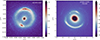 |
Fig. 1. Images of the two strong gravitational lensing systems used in this paper, where subhalo detections (marked by a white cross) have been claimed in previous works. Left: image of B1938+666 taken in the K′ band by NIRC2 on Keck. In this case, zL = 0.881 and zs = 2.059; the pixel and FWHM (determining the resolution) scales are 10 and 70 milli-arcseconds (hereafter, mas), respectively. Right: HST F814W observations of the lens J0946+1006. For this system, zL = 0.222 and zs = 0.609; the pixel size and resolution are 50 and 90 mas, respectively. See Table 1 for a list of previous analyses of these systems. |
Summary of most relevant works in which the two systems considered here have been modelled – with or without the perturber.
3.1. JVAS B1938+666
The B1938+666 system was observed as part of the Jodrell Bank VLA Astrometric Survey (JVAS; Patnaik et al. 1992), and discovered to be a gravitational lens based on near-infrared HST imaging (King et al. 1997). In addition to the original NICMOS/NIC1 F160W HST observations (PropID 7255: PI Jackson), the lens system was observed by the WFPC2 and NICMOS/NIC2 instruments on HST in the F555W, F814W, and F160W bands (PropID 7495: PI Falco). The lens and source redshifts are zL = 0.881 and zs = 2.059 (Tonry & Kochanek 2000; Riechers 2011). In this paper, we use higher-angular-resolution observations that were obtained using the adaptive optics (AO) system at the Keck Telescope. These K′ data were obtained with the NIRC2 instrument as part of the SHARP Phase 1 sample and were used for both smooth mass models of the lensing galaxy (Lagattuta et al. 2012) and the analysis by Vegetti et al. (2012), who first discovered the presence of a dark perturber at the location of the brightest part of the northern arc, modelling it with a PJ profile and obtaining a subhalo mass of Msub = 1.8×10⁸ M⊙. To date, this is the lowest mass of (sub)halo detected via gravitational imaging. They calculated 3σ limits in magnitude and luminosity of MV>−14.5 and LV<5.4×10⁷ LV,⊙. Despite the lower subhalo mass, the limits on its luminosity are not very stringent because the perturbation is detected in a luminous part of the arc, and it is thus not possible to distinguish its potential emission from the arc. As reported in Vegetti et al. (2012), the limit was estimated by calculating the quadrature sum of the pixel noise in a 16×16 pixel square aperture, chosen to match the tidal radius of the substructure, and then applying a K-correction to convert the K′ value in a rest-frame V band limit.
Şengül & Dvorkin (2022) analysed the lower-resolution HST observations of this system and measured the slope of the subhalo density profile, finding a best-fit value of γsub = 1.96±0.12, which corresponds to a concentration of ∼60. The inner slope is thus close to isothermal, and the concentration is high compared to the theoretical prediction for this mass range. They also considered the possibility that the perturbation is caused by an isolated dark halo along the line of sight. They included the redshift as an additional free parameter and found a preferred redshift of  , thus preferring a line-of-sight halo over a subhalo. Recently, Tajalli et al. (2025) modelled the redshift of the perturber using the higher-resolution Keck data, finding a preference for an object in the foreground at z = 0.13±0.07. Here, we do not explore this possibility since we are interested in comparing different profile models with simulated subhaloes in hydrodynamical simulations.
3.2. SDSS J0946+1006
We use observations of the gravitational lens system J0946+1006 observed by the ACS camera on board the HST as part of the SLACS sample (Bolton et al. 2006). Observations have revealed the presence of three lensed sources: two arcs visible in HST observations (Gavazzi et al. 2008) zs1 = 0.609 (inner lensed arc) and zs2 = 2.035 (outer lensed arc, Smith & Collett 2021) and an additional higher-redshift source at zs3 = 5.975 detected with MUSE (Collett & Smith 2020). In this work, we consider observations in the F814W band and model the inner arc, which also is the one with the highest signal-to-noise ratio. The detection of a dark perturber of mass Msub = 3.51×10⁹ M⊙ in the north-west part of this arc has been claimed first by Vegetti et al. (2010b). They also calculated a 3σ upper limit luminosity of the subhalo of LV<5.0×10⁶ LV,⊙. Based on the residual images, they determined an upper limit on the magnitude of the substructure in two different ways: by setting the limit equal to three times the estimated (cumulative) noise level or by aperture-flux fitting, both inside a 5x5 pixel window. The aperture is chosen to gather most of the light of the substructure, which is expected to be effectively point-like given its low mass. Its presence and location were later confirmed by other works (Minor et al. 2021; Nightingale et al. 2024; Ballard et al. 2024; Enzi et al. 2025), while the estimates of its total mass and properties depend on the assumptions made for the subhalo profile (see Table 1). The original detection has been modelled with a PJ (Jaffe 1983; Muñoz et al. 2001) profile that produces a very compact mass distribution and is thus very efficient as a lens. Other works instead described the subhaloes as NFW profiles (classic or truncated). Due to the shallower inner slope, these require a higher total mass to produce a lensing effect of the same magnitude. Indeed, Nightingale et al. (2024) finds a total subhalo mass ∼1011 M⊙ by calculating  and assigning it a concentration c200 following Ludlow et al. (2016). Their findings are compatible with the predictions from Despali et al. (2018): the mass of an NFW profile (following a concentration–mass relation) must be one order of magnitude larger than a PJ subhalo to produce a lensing effect of the same scale. Minor et al. (2021), Ballard et al. (2024) and Enzi et al. (2025) have instead considered the concentration as an additional free parameter in the NFW profile, finding best-fit values that are extreme outliers of the CDM model. Finally, Enzi et al. (2025) and Tajalli et al. (2025) also modelled the redshift of the perturber, confirming that it lies very close to the redshift of the lens, thus preferring a substructure over a halo along the line of sight.
Parameters of the detected subhaloes.
4. Results of lens modelling
We model the two considered systems with the PRONTO code, as is described in Sect. 2.1. We first model the main lens, including both the central galaxy's mass and light, finding lens parameters consistent with previous works. We then add a second mass component to describe the perturber and test the density profiles listed in Sect. 2.2. In each case, we calculate the posterior distribution of the lens and subhalo parameters simultaneously using MULTINEST (Feroz et al. 2013), using 288 live points, an evidence tolerance equal of 0.5, and a sampling efficiency of 0.8. In this section, we focus on the posterior distributions of the subhalo parameters and their physical interpretation while we show the full posteriors, the best lens models and reconstructed sources in the appendix (Figs. A.1–A.5).
The best-fit parameters describing the subhaloes and the associated errors are listed in Table 2: these are the mean values and 95 confidence intervals calculated by MULTINEST. The third column reports the logarithmic difference in Bayesian evidence between the perturbed and smooth model Δlog E=log Epert−log Esmooth: a positive difference indicates that the perturbed model is preferred over the smooth case. In most cases, the additional mass component significantly improves the Bayesian evidence of the model.
4.1. Inferred properties of the detected subhaloes
Figures 2, 3, and 4 report the posterior distributions of the subhalo properties for the PJ, NFW, and PL profiles. The right panels of Figs. 2 and 3 show the analytic density and enclosed mass profiles corresponding to the best-fit subhalo parameters; we discuss these in detail in Sect. 4.2.
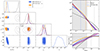 |
Fig. 2. Left: nested sampling posterior distributions for parameters describing the subhalo in the system B1938+666 for the PJ (orange) and NFW (blue and gray) profiles. In all cases, we fit for the subhalo mass Msub (in M⊙) and position (xsub and ysub, measured in arcseconds with respect to the centre of the image). We also plot the posterior of the subhalo position of the PL profile (purple), while the other parameters describing the models are plotted separately in Fig. 4. We consider two variations of the NFW profile: one (grey) where the concentration csub is fixed by the concentration–mass relation from Duffy et al. (2008) and a case (blue) where csub is left free to vary. The best-fit values derived from the posteriors are listed in Table 2. Note that we plot the mass Msub in logarithmic space for better comparing the model, and this may give the impression that the grey contours are reaching the edge of the prior, which is not the case. The black rectangle in the (xsub−ysub) panel indicates the pixel scale of the data. The best lens model and reconstructed source for the smooth and smooth+NFW cases are shown in the Appendix in Figs. A.1 and A.4 shows the posterior distribution for all parameters in all considered models. Right: radial density and projected enclosed mass profiles corresponding to the best-fit subhalo profiles in the left panel, i.e. to the values reported in Table 2 (mean and 95 CL). The profiles are calculated analytically following the definitions in Sect. 2.2. The vertical dashed lines in the top panel mark the slope transition for the NFW and PJ profiles, i.e. rs and rt. In the bottom panel, the dotted lines mark the distance at which the PJ, NFW and PL curves intersect, thus predicting the same mass, i.e. req = 0.9 kpc. The grey areas show the data resolution. |
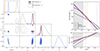 |
Fig. 3. Same as Fig. 2 but for the lens system J0946+1006. Here, the NFW profile with concentration fixed by the concentration–mass relation is a worse fit to the data than the other models: a symptom is the best-fit position of the subhalo, which is very different and more uncertain than for the other profiles. Moreover, the enclosed mass in the bottom-right panel does not converge within a radius similar to the other two profiles, i.e. Req = 0.45 kpc. The best models and the full posterior distributions can be found in the appendix in Figs. A.1 and A.5. |
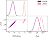 |
Fig. 4. Posterior distribution of the PL model parameters: the slope, γsub, and the convergence normalisation, log(κsub), measured in arcseconds. The dashed lines mark the slope of an isothermal profile. |
In the case of B1938+666, all four profiles significantly improve the Bayesian evidence compared to the smooth model (see Table 2), with the NFW profile with fixed concentration being the least favourite model. The inferred subhalo positions, left free to vary, are consistent within the resolution of the data (70 mas), indicating the stability of the detection. The position is consistent with Vegetti et al. (2012). For J0946+1006, the PJ, PL, and NFW profile with free concentration also improve the Bayesian evidence of the model, and the NFW profile with fixed concentration is again the least favourite model. We note how the inferred subhalo position for this model also differs by more than 2σ from the other profiles. In this case, the inferred subhalo mass is extremely high, and it cannot correspond to a dark structure. This result is compatible with the highest mass value (and the corresponding subhalo position) calculated by Nightingale et al. (2024). In practice, an object with such a high mass cannot lie very close to the arc because it would modify the lensed images far from the detection location and is thus forced to move (see Fig. A.3 for the results of the fit with different NFW profiles). For the other three profiles, the subhalo position is instead consistent within the resolution (90 mas) and with Vegetti et al. (2010a).
While the PJ and NFW models have fixed values for the inner and outer density profile slopes, when we model the perturbers with a (not truncated) PL profile, the slope is left as a free parameter. In practice, this is defined as in Equation (2), but assuming spherical symmetry (q = 1). Fig. 4 shows the resulting posteriors for the subhalo convergence normalisation κ0 and inner slope γsub. In both lenses, the subhalo position agrees with the results of the PJ and NFW profiles (see also Fig. 6 and the appendix). The extremely compact detection in B1938+666 is best described by a profile with γsub=−2.44±0.17, steeper than isothermal and than all profiles considered so far. The inferred slope in J0946+1006 is instead γsub=−2.1±0.11, which is still compatible with the isothermal slope and thus with the PJ and mNFW profiles.
Given the intrinsic difference among the adopted profiles and mass definitions, the inferred subhalo mass differs, and our measurements are consistent with the trends in previous works, reported in Table 1. When the concentration is left free to vary, the resulting best-fit NFW profiles are very compact, leading to large concentrations, consistent with previous works: csub = 257±70 in B1938+666 and csub = 201±38 in J0946+1006. In practice, this means that the classic NFW profile is not a good description of the properties of the detections: to reproduce them, the scale radius rs becomes artificially small, leading to extreme values of concentration. To aid the comparison with theoretical predictions, in Fig. 5, we plot the values inferred from the observational analysis together with the concentration–mass relations measured in numerical simulations (Duffy et al. 2008; Ludlow et al. 2016; Diemer & Joyce 2019; Moliné et al. 2017). By construction, the results obtained with a fixed concentration-mass relation – our black points and the results from Nightingale et al. (2024) – lie on the analytical predictions, while all the other measurements show a clear departure from the numerical predictions. We note, however, that all these concentration-mass relations result from fitting the dark matter profiles of haloes in simulations that do not include the effect of baryons, which may be especially relevant at the mass scales corresponding to the detection in J0946+1006. Mastromarino et al. (2023) measured the concentration-mass relation in the Eagle cold and SIDM runs (Robertson et al. 2021), comparing the dark-matter-only and hydro values. At the scale of galaxies with masses M200>1012 M⊙, the hydro concentrations are higher by a factor of 2–3 compared to the dark-matter-only case. It is not possible to extrapolate their results to the mass range considered here. Still, their results suggest that the presence of baryons would not increase the mean concentration enough to reproduce our values inferred from observations. In Sect. 5, we compare our results to the subhaloes of TNG50-1, which combines high-resolution with advanced treatment of baryonic physics.
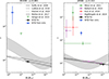 |
Fig. 5. Comparison of the NFW models from our analysis (black circles and blue squares) and previous works with concentration–mass–redshift relations derived from N-body simulations. All results are expressed in terms of the virial mass of haloes Mvir, except for Moliné et al. (2017) who measured the relation using M200, i.e. the mass within the radius enclosing an overdensity of 200. In this case, the relation has an additional dependence on the distance of the subhalo from the centre of its host halo. Since the observational results are derived in projection (on the lens plane), we cannot determine the three-dimensional distance from the host centre, and we plot a range of relations for distances between 0.1Rvir and Rvir. Given that it was calibrated on subhaloes rather than isolated haloes, it naturally predicts higher concentrations at the low-mass end. In each panel, the coloured symbols and error bars show our inferred values from the analysis of the observations (black circle and blue square) and the results from previous works (empty symbols), listed in Table 2. Şengül & Dvorkin (2022) used a fixed mass Msub = 109 M⊙ and varied the inner slope of the profile (that we report in the table), from which they estimated a corresponding concentration but did not provide uncertainties in this quantity. |
4.2. A radius of equal enclosed mass
Interestingly, the PJ, PL, and NFW (with free concentration) profiles are preferred over the smooth model at roughly the same level (see Table 2), meaning that they can fit the images equally well despite their structural differences. To investigate the reason behind this, we look at their density and enclosed mass profiles, plotted in the right panels of Figs. 2 and 3. The grey bands mark the resolution of the data, calculated as the FWHM of the PSF (divided by two, given that we are looking at a radial profile). For the PJ and NFW profiles, the steeper inner part of the density profiles is thus close to the resolution of the data in both cases: in B1938+666, both rt and rs are unresolved, while in J0946+1006, they lie right above the resolution limit. This means that the lensed images can resolve the profiles in the slope transition region and above but not in the innermost part. The untruncated PL profiles produce an inner slope between the two models. In the bottom panels, we plot the projected enclosed mass M2D(<R): this is especially important since gravitational lensing robustly measures the projected mass distribution – which we then convert to a 3D profile. For all models that cause a significant increase in the Bayesian evidence of the model, the enclosed mass profiles intersect at roughly the same distance Req from the subhalo centre: Req = 0.9 kpc for B1938+666 and Req = 0.45 kpc for J0946+1006. Note that Req encloses almost the total mass of PJ profiles, while the NFW and PL have a larger fraction of the mass in the outer parts. A counter-example is the NFW profile with a fixed mass–concentration relation in J0946+1006, which is a worse fit and does not converge to the same enclosed mass within the same radius. We can conclude that all subhalo models are trying to fit the enclosed mass within Req rather than the inner slope, which is not resolved.
To investigate the nature of Req, in Fig. 6 we visually compare all models in the lens plane, looking at their impact on the critical lines around the location of the perturbations. Each model is represented by a different colour (that matches Figs. 2 and 3) and line style, and the inferred subhalo position is marked by crosses of the corresponding colour. The white circles show Req. Moreover, we use equation (3) to calculate the Einstein radii of the PL model, represented by the dashed purple circle. In the case of B1938+666 (left panel), the three best-fitting profiles produce an extremely similar effect that is needed to fit the very compact mass distribution of the subhalo, while the NFW model with fixed concentration barely modifies the critical lines with respect to the smooth model. The perturber in J0946+1006 (right panel) is more massive, and thus produces a larger variation in the critical lines, with a visible difference between the models. Here, we also compare to the results by Minor et al. (2021) who modelled the same system: with their model, they inferred a robust radius δθc = 1 kpc, defined by Minor et al. (2017) as the radius within which the mass measurements is robust. We plot it here as the dashed white circle – assuming as a centre our best-fits subhalo position (which may differ from their original result). Interestingly, the three radii plotted here do not match: it is intriguing that Req does not yet correspond to an obvious quantity related to gravitational lensing theory. However, δθc also depends on the macro model, and thus part of the difference between their value and ours could be due to the difference in the underlying mass distribution of the lens. It is reasonable that detectable perturbations would robustly characterise the projected surface mass density at their location. A more systematic analysis is needed to identify its nature, given that it would allow us to interpret the detections without the need to impose a density profile model. We investigate this scale in a follow-up paper.
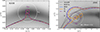 |
Fig. 6. Zoom on the location of the two detections to highlight the differences in the critical lines and subhalo position between the considered models (lines and crosses of the corresponding colour). The circles marks (i) the radius, Req, at which the PJ and NFW profiles produce the same enclosed mass (solid white), (ii) the Einstein radius, Rein, calculated with Equation (3) for the PL profile (purple), (iii) the size corresponding to the robust mass defined for J0946+1006 by Minor et al. (2021, dashed white). In the case of B1938+666, the perturber is very compact, and the three best models have very similar critical lines. In J0946+1006, the larger subhalo mass translates into larger visible differences among the models. |
5. Comparing observations and simulations
In this section, we use the TNG50-1 simulation to compare simulated subhaloes with the results of the previous section. H23 already showed that the classic NFW model does not provide a good description of subhalo density profiles in TNG50 because the measured inner logarithmic slopes are steeper, and the NFW cannot model the external truncation. This is due to the combined effects of baryons at the centre of satellites and haloes and tidal stripping. In this section, we search for simulated analogues of the two detections, compare to the results of Minor et al. (2021) and discuss their properties in terms of density profiles, projected mass, stellar content, merger history, and lensing effect.
Minor et al. (2021) used the TNG100-1 simulation, while we can count on the higher-resolution TNG50-1 run: the spatial resolution, defined by the gravitational softening, improves from ϵDM,* = 0.74 comoving kpc to ϵDM,* = 0.28 comoving kpc; similarly, the dark matter particle masses decreases from mDM = 7.5×10⁶ M⊙ to mDM = 4.5×10⁵ M⊙. This provides us with a better resolution at the centre of haloes, and we are able to measure density profiles down to lower halo masses. However, all simulations are prone to numerical effects, and we discuss our limitations in Sect. 5.4. We chose the simulation snapshots that are closest to the lens redshift, zL, of each lens: snapshot 84 at z = 0.2 and snapshot 53 at z = 0.89.
5.1. Finding analogues of the detections in CDM
We start by comparing the inner slopes inferred from the data with the PL model (see Fig. 4) to those of simulated subhaloes. We used the inner slopes calculated in H23 by fitting a modified Schechter profile to the simulated data, i.e. a PL profile with exponential truncation. The two panels of Fig. 7 show the cumulative and differential distribution of subhalo slopes in different mass bins. Here, we use all TNG50 subhaloes, independently of their host halo mass, to determine how common the inferred slope is in the entire population. As is discussed in Sect. 2.3, we consider only satellites as subhaloes and did not consider the isolated haloes in the SUBFIND catalogue. In addition, we choose two bins corresponding to the inferred mass ranges for the two detections (see Table 2). The distribution for subhaloes with Msub<4×10⁹ M⊙ is essentially identical to that of the entire population, while the distribution for the higher mass bin moves to shallower slopes. When looking only at density slopes, the detection in J0946+1006 is thus compatible with the slopes of 25.6 per cent of subhaloes in the range 4×10⁹ M⊙≤Msub<5×10¹⁰ M⊙. The perturber in B1938+666 is instead more compact and has a steeper – and thus rarer – profile slope that is compatible with 8.8 per cent of subhaloes in the lower-mass range, 4×10⁸ M⊙≤Msub<4×10⁹ M⊙.
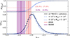 |
Fig. 7. Comparison between the γsub inferred from observations with the PL model (see Fig. 4) and the inner slopes of subhaloes from the TNG50-1 simulation. In the latter, the slope has been measured for all subhaloes in H23 (see their Fig. 9). The bottom panel shows the distribution of slopes of all subhaloes (black) and two mass bins roughly corresponding to the range of the detections. The coloured vertical lines and shaded areas correspond to the observed values (Table 2). In the top panel, we show the cumulative distribution for all subhaloes and the second mass bin, and we report the corresponding fractions of subhaloes that are compatible with the observed slopes in the two mass bins, highlighting the one that better corresponds to the detection in each case with the horizontal lines and corresponding numbers. |
However, this comparison is not yet complete, since we have shown in Sect. 4.1 that the subhalo profiles must match not only in terms of slope but mostly in the enclosed mass. Moreover, the histograms are binned using the total subhalo mass, while the most robust mass measurements through lensing correspond to the enclosed mass within the radius at which different profile definitions converge (see Figs. 2 and 3).
We now proceed to a more thorough comparison in the parameter space of projected quantities. We adopted the definitions of Minor et al. (2021), who used γ2D(Rc) and M2D(<Rc), i.e. the average log-slope of the surface density profile around a characteristic radius and the projected mass within the same distance. In the case of B1938+666, we chose Rc=Req = 0.9 kpc, since this scale corresponds to ∼5.9ϵDM,* at z = 0.881, and thus is reasonably well resolved. In the case of J0946+1006, Req = 0.45 kpc = ∼1.9ϵDM,* at z = 0.222, which is not enough to guarantee good convergence, as we discuss in more detail in Sect. 5.4. In the latter case, we thus choose the same value adopted by Minor et al. (2021), Rc = 1 kpc; this has the advantage of being both reliable in terms of resolution and comparable to their work.
We calculate γ2D(Rc) and M2D(<Rc) from the PJ, NFW, and PL analytical profiles that best fit the observational detections, i.e. those shown in Figs. 2, 3 and 4 and corresponding to the values in Table 2. In the simulation, the projected mass within the chosen radius M2D(<Rc) is calculated by summing up the masses of all subhalo particles that lie within a cylinder with a radius, Rc, from the centre of the subhalo. The average 2D log-slope around the characteristic radius γ2D(Rc) is calculated by computing the surface density profile around Rc using five bins consisting of cylindrical shells and fitting a power law to the data points (the considered range is shown by the purple band in the bottom panel of Fig. 8). Both quantities are computed for 1000 random orientations to account for potential biases due to projection effects. Moreover, we compute the average values for the top 10 percent lines of sight with the highest values of γ2D(Rc) and M2D(<Rc) respectively. Minor et al. (2021) only considered subhaloes hosted by haloes of Mhalo∼1013 M⊙, i.e. the typical mass of lens galaxies. Given that the simulation provides us with a (50 Mpc)3 volume instead of (100 Mpc)3 – and thus fewer objects – we relax the selection criteria to include larger statistics and consider host haloes with total masses of 5×10¹²−5×10¹³ M⊙ and stellar masses of 1010−1013 M⊙. Mastromarino et al. (2023) show that haloes selected in this range of viral masses have a distribution of Einstein radii similar to that of observed lens samples.
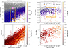 |
Fig. 8. Top: log-slope of the surface density profile around r=Req = 0.9 kpc (for B1938+666) or r = 1 kpc (for J0946+1006) against the projected total mass enclosed within the same distance. See Fig. 13 for the J0946+1006 results at r=Req, which we believe are affected by resolution. The coloured points indicate the top 10 percent of lines of sight that yielded the largest density values, colour-coded by the stellar-to-total mass ratio. The grey dots indicate the averages over all 1000 lines of sight. The larger points show the slope and mass values inferred from our lens modelling for the PJ (orange circle), NFW with free concentration (blue diamond) and PL (pink square) profiles. In the right panel, we also compare to the measurement by Minor et al. (2021). Bottom: total subhalo mass as a function of the enclosed projected mass. Points are coloured by the total stellar mass of the subhalo. The mean and standard deviation used in Equation (11) are represented by the solid and dotted black lines. |
The top panel of Fig. 8 shows the comparison results in the parameter space defined by γ2D(Rc) and M2D(<Rc): the grey points show the averages taken over all lines of sight, while the top 10 per cent values are coloured by the fraction of stellar mass of each subhalo. On the left, we see that many subhaloes match the NFW profile that best fits the detection in B1938+666. The PJ and PL profiles are also compatible with simulated subhaloes, although they lie at the edge of the distribution. However, we must note that there is a large difference between the grey and coloured points, indicating that high-density projections are needed to reproduce the observed results. The subhaloes are dark-matter-dominated, i.e. with a fraction in stellar mass lower than ∼5 per cent. In the right panel, we are able to find a few subhaloes matching the inner slope predicted by the PL and NFW profiles for the detection in J0946+1006. In this case, the fraction of stellar mass of the subhaloes is higher but still less than 15 per cent. These are close to the constraints from Minor et al. (2021), represented by the black cross. However, they did not find any good match when performing the same measurements on the TNG100-1 subhaloes, concluding that this detection is an outlier of CDM. As we discuss in more detail in Sect. 5.4, we believe that the difference in our results is explained by the better resolution of TNG50-1, which allows us to measure the inner density profiles of subhaloes more reliably.
5.2. Properties of the simulated analogues
To highlight the range of subhalo properties that could match the detections, we now look at their total and stellar masses, density profiles, luminosities, and merger histories. In the bottom panels in Fig. 8, we plot the total subhalo mass Msub as a function of M2D(<Rc) and colour the points by their stellar mass. For both systems, a certain value of M2D(<Rc) corresponds to total subhalo masses that span one order of magnitude. Moreover, while the total stellar masses are low for the B1938+666 detection (M*≤106.5 M⊙), those required to match the properties of J0946+1006 are higher (108.5 M⊙≤M*≤1010 M⊙) and thus may be problematic for a subhalo detection that does not correspond to a visible satellite. We fit the mean linear relation between the total and projected mass as

finding (A,B) =(−3.95±0.2,1.65) in the left panel and (A,B) =(−0.08±0.4,1.13) in the right one. These are plotted as solid (mean) and dotted (standard deviation) black lines.
We now select simulated subhaloes that lie close to the detections in the plane defined by γ2D(Rc) and M2D(<Rc) and investigate their properties more in detail. The selection of such analogues is shown by the orange boxes in the top panels of Fig. 8: for B1938+666, we chose subhaloes that match the whole range of 2D slopes between the NFW and PJ results, given that they all correspond to dark-matter-dominated structures; for J0946+1006, we instead excluded systems that match the PJ slope, given that they are all baryon-dominated (M*/Msub>0.5). First, we compare the luminosities of simulated subhaloes to the upper limits that have been estimated from observations: LV<5.4×10⁷ LV,⊙ for B1938+666 and LV<5×10⁶ LV,⊙ for J0946+1006. We use the absolute magnitudes in V band (Buser 1978) provided in the TNG50-1 subhalo catalogue based on the summed-up luminosities of all the stellar particles of each subhalo. In this calculation, we did not include any extinction effect by dust, which may lower the luminosities presented here. We think that this simplifying assumption does not significantly influence our conclusion, since (i) the two host lens galaxies are massive ellipticals and no dust effect (such as a dust lane) is observed in the lensed images and (ii) the subhaloes lie away from the luminous part of the lens galaxy. However, this is a potential source of systematics. The resulting values for the analogues are shown in Fig. 9 as orange circles and compared to the general population of subhaloes (black dots). In both cases, the analogues of the detection have higher luminosities than the mean population, and this is particularly evident in the case of J0946+1006 (right panel). While the left panel shows that all analogues are compatible with the upper limit set for B1938+666, on the right, we see the opposite: all simulated analogues are too bright to correspond to the subhalo in J0946+1006. As discussed in Sect. 3, we point out that the upper limit is more stringent for J0946+1006, given that the detection is located in a relatively dark part of the image, while it could be not as accurate for B1938+666. Nevertheless, this confirms that the subhalo detection in J0946+1006 is in tension with the predictions from numerical simulations. These considerations may not hold if the detected object was an isolated halo along the line of sight and not a subhalo: the simulated luminosities may change, as well as the observational limits, since an object further away from the lens may be harder to see; moreover, the mass and concentration of an isolated halo may differ from the values calculated from subhaloes. The possible effect of dust is thus mostly relevant for J0946+1006, where the simulated values may be lowered and brought in agreement with the observational limit. We note however that, for this to happen, the observed luminosity should decrease by more than two orders of magnitude.
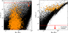 |
Fig. 9. Comparison of the luminosity of the simulated subhaloes and the observational limits set for the two detections. First, we selected the systems that best match the observational inference in terms of projected slope and enclosed mass: in practice, these were selected within the orange rectangles in the top panels of Fig. 8. We computed their luminosity, LV, from the V-band magnitudes provided in the TNG50-1 subhalo catalogue and plot them as orange circles as a function of the subhalo mass, Msub. We show the results for B1938+666 on the left and J0946+1006 on the right. The black dots show instead the luminosity of the general subhalo population at the same redshift. The observational upper limits (see Sect. 3) are represented by the horizontal red line in the plot. |
We then plot the density profiles of the analogues in Fig. 10 and compare them with the analytical profiles from Figs. 2 and 3. As was found in many previous works, the population of low-mass subhaloes (left panel, matching the B1938+666 detection) spans a wide range of properties due to the diversity in accretion history and tidal disruption. We also note that, for some systems, the inner part of the density profile may be affected by low particle number, even if we are well above the spatial resolution limit – we discuss this in more detail in Sect. 5.4. In the right panel, we see that the selected subhalo profiles nicely reproduce the blue curve (i.e. the NFW profile inferred for the J0946+1006 detection) well beyond the region that was used to measure the inner slope. At the same time, the subhaloes present a wide range of truncations in the outskirts, signalling different levels of tidal stripping and, possibly, infall times, as already reported in H23. To investigate this hypothesis, we analyse the subhalo merger trees, already described in Sect. 2.3. For each object, it is possible to walk the tree backwards to determine when it formed as an independent structure and when it then fell into the host halo. Here, we want to compare the infall properties of subhaloes identified as possible analogues of the detections to the general population of subhaloes in the same mass range and at the same redshift. We select the main haloes that host the analogues and follow the merger trees of all their subhaloes in the mass ranges: 2×10⁸ M⊙≤Msub(z = 0.89)≤5×10⁹ M⊙ for B1938+666 and 109 M⊙≤Msub(z = 0.2)≤4×10¹¹ M⊙ for J0946+1006. We plot the distribution of infall redshift and mass for the analogues (orange) and the entire population (grey) in Fig. 11. For B1938+666, the distribution of infall redshifts, zinf, is similar for the analogues and the general population, while the infall masses Minf of the analogues show a clear peak. The effect is more prominent for the detection in J0946+1006, where we find a difference in the distribution of infall times that excludes some of the most recent mergers, and Minf shows a clear preference towards very high masses. This means that the observed subhaloes are only compatible with descendants of more massive structures that may host a baryonic core and that have been subjected to stripping during their life in the host halo. Both these effects contribute to creating the observed compact mass distributions. However, as is seen in Fig. 9, subhaloes with infall masses corresponding to J0946+1006 are indeed too massive and contain too many stars to be an actual counterpart of the detection.
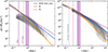 |
Fig. 10. Subhalo density profiles of the simulated subhaloes that best match the observational inference (B1938+666 on the left and J0946+1006 on the right), i.e. the same shown in orange in Fig. 9. The purple band shows the radial range used to measure the slope, γ2D, for Fig. 8. The vertical lines mark the softening of the simulation (vertical solid line), and the value commonly used in simulation as a reliable resolution limit (i.e. 2.3ϵDM,*, vertical dashed line) and the resolution of the observational data. |
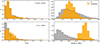 |
Fig. 11. Properties of simulated subhaloes at infall. We used the merger trees to track the subhalo evolution and measure their properties at infall, i.e. at the redshift where they first entered their host halo. We plot the normalised distribution of infall redshifts zinfall (left) and the mass at infall Minfall (right). The orange histograms show the distribution of the subhaloes selected as analogues, i.e. those lying within the orange boxes in the top panels of Fig. 8 for which we show the density profiles in the bottom panels of the same figure. The grey histograms show instead the distribution for all subhaloes in the same host haloes and with final masses between 2×10⁸ M⊙≤Msub(z = 0.89)≤5×10⁹ M⊙ for B1938+666 and 109 M⊙≤Msub(z = 0.2)≤4×10¹¹ M⊙ for J0946+1006. |
5.3. Einstein radii of the subhaloes
Given the results of the previous section, it is clear that subhaloes of a given total mass can produce a range of lensing effects, depending on their density profiles. H23 found that the mNFW model describes the average density profile of subhaloes, but individual subhaloes within the same mass bin differ in terms of inner slope and concentration. The spread correlates with other subhalo properties, such as the infall time or the baryonic content. Given that the lensing effect is directly dependent upon the density distribution, it is natural to expect a spread in the lensing properties of subhaloes as well. Here, we extend their results by calculating scaling relations for the subhalo Einstein radius, Rein, as a function of subhalo mass, Msub, and the circular velocity peak, Vmax. We chose a lensing configuration with the lens (the subhalo) at a redshift of zL = 0.2 and the source at a redshift of zs = 0.609, corresponding to J0946+1006. We undertake separate analyses for the smoothed particle surface density maps created from (i) the particle data and (ii) the best mNFW profile fits of each subhalo. Here, we present the latter and discuss the potential biases introduced by the spatial and mass resolution of the simulations when using only particle data in Sect. 5.4. To analyse the lensing effect of the analytical mNFW profiles, we integrate the best-fitting spherical density profile in the z direction to obtain a surface density profile, and = we construct a circular map of 20482 pixels with a field of view of 2rs. In order to resolve the Einstein radii of subhaloes with very different radial extents, the field of view of the ray tracing computations (which is only a part of the total field of view of the entire surface density map) is adaptive – to a minimum of 0.1 arcseconds depending on rs, and within this field of view, 20482 rays are traced. We find the (equivalent) Einstein radius Rein by measuring the area enclosed by the tangential critical line and computing the radius of the circle that has the same area, following the approach of Meneghetti (2022).
Fig. 12 shows the resulting distribution of Rein as a function of subhalo mass and Vmax. Here, instead of the subhalo mass, Msub, obtained from the particle data, we compute the subhalo mass Msub,mNFW by integrating the analytic profile. This is necessary to reach the small scales corresponding to the Einstein radii of the subhaloes. As can also be seen in Fig. 10, it is well known that the inner parts of the density profiles are affected by artificial core formation (see also the next section) which would lower the density and thus the lensing power. We thus use the analytical best-fit profiles to integrate the projected mass and calculate the Einstein radius. In this way, it is possible to look at subhaloes with low mass and small Einstein radii that would otherwise not be properly resolved due to resolution limitations. This does not mean that the density profiles of subhaloes (and the associated fits) are free from noise, which is also represented by the large scatter at low masses. However, integrating the analytical profile does not introduce a significant bias in the total projected mass in the mass regime we are interested in (Msub≤1011M⊙) – see the appendix for a more detailed discussion.
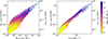 |
Fig. 12. Scaling of the Einstein radius (obtained from the best mNFW fits) with subhalo mass (left) and Vmax (right). In both plots, the colour-coding of the data points indicates the subhalo stellar mass M*. The cyan lines represent the best power law fit for all of the data points. |
Despite the clear correlation, we see a significant scatter around the mean at fixed subhalo mass or at fixed Rein. Gravitational lensing robustly measures the projected mass in the region covered by the lensed images, while the total subhalo mass is inferred via a model for the density profile. These results show how using a mean profile (such as the NFW or the mNFW) may not be sufficient to interpret lensing data, given that a certain Einstein radius could match a wide range of total masses. Moreover, subhaloes with lower Rein may simply become non-detectable (although present), and the more lensing-efficient ones will dominate the sample. The light blue line represents the best-fit relations. For the top panels, they are given by:
Generally, the scaling relations values also depend on the redshifts of the lens and source. However, the lens and source configuration do not strongly affect the slope of the relations. Because of the Vmax−Msub relation, the scaling of Rein with Vmax is not surprising, but the scatter of the Rein−Vmax relation turns out to be much smaller than for the Rein−Msub relation.
5.4. The effect of resolution
It is well known that measurements from simulations can suffer from numerical uncertainties if performed at scales close to the spatial resolution or using low-mass (sub)haloes that are traced by a few particles. Moreover, low-mass subhaloes at the limit of resolution can be subjected to artificial disruption, altering their predicted number and properties (van den Bosch et al. 2018; Green et al. 2021). Here, we do not try to correct potential artificial disruption and use the TNG50-1 subhalo catalogues as they are. In this section, we thus present tests that we performed to quantify possible resolution limitations of our analysis (beyond what already discussed in the previous sections) and the strategies to circumvent them.
As is described in Sect. 5.3, we calculated the subhalo Einstein radii both directly from the particle distribution and from the analytical profiles. Using the latter allowed us to partially circumvent resolution systematics and study a larger range of subhalo lensing properties (shown in Fig. 12) compared to the results obtained from discrete particle data. For the particle data, we used PY-SPHVIEWER (Benitez-Llambay 2015) to create surface density maps of 20482 pixels for each individual subhalo. For each map, we chose a camera looking at the subhalo from infinity so that the map is rendered using a parallel projection. The field of view was chosen so that every particle of the subhalo is still contained within the map. Based on the position of 32 neighbouring particles, the smoothing length was calculated for each individual particle, and the minimum smoothing length was set to the softening length of TNG50. The density values of each pixel were normalised such that the total mass of the subhalo equals the sum of the pixel values. The side length of the field of view for the ray tracing was set to 2 arcseconds, and 5122 rays were traced within it. In Fig. 13, we now compare those measurements (here in grey) to the Einstein radii derived from the particle data. Given the limits imposed by the discreteness of the particle distribution and by the resolution of the simulation, it was, in fact, possible to reliably measure Rein only for subhaloes with Msub≥1010 M⊙. In this range, the overall distribution of points looks similar, but the values calculated from the particle distribution have a larger scatter, particularly towards small values of Rein. In the Rein−Vmax space, it is particularly clear that the data points below the softening length ϵDM,* are those that deviate the most from the relation obtained from the analytic profiles. For the analytical profiles, the limitations are instead determined by the number of pixels in the surface density maps, the field of view and the number of rays in the ray tracing computation. These limitations can lead to a small amount of artificial scatter for a few low-mass subhaloes with small Einstein radii, which can be mitigated by increasing the resolution even further. However, this is less significant than the intrinsic resolution limits of the simulations.
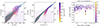 |
Fig. 13. Tests of the impact of numerical resolution on our results. Left and central panel: comparison between the Einstein radii obtained from the best modified NFW profile fits (in grey – corresponding to the points in Fig. 12) and those calculated from the smoothed particle surface density maps, coloured by the subhalo stellar mass. The cyan lines are the best power law fits for the latter. In both plots, the regime below the softening length is coloured purple. Right: repeat of the measurements performed for Fig. 8, using Req = 0.45 kpc for the lens J0946+1006. |
A similar resolution effect can also affect our measurements of the projected mass and slope presented in Fig. 8. Here, we repeat the measurement at the redshift of J0946+1006 using Rc=Req = 0.45 kpc instead of Rc = 1 kpc. As is discussed in Sect. 5.1, this value is close to the spatial resolution limit of the simulation, and thus our measurement of the projected slope γ2D, based on five radial bins around Rc may be biased. The results are shown in the right panel of Fig. 13, which should be compared to the top-right panel of Fig. 8. Indeed, the slopes measured at this inner radius are shallower because of the artificial core of the central part of the profiles, highlighting the need to be careful in the treatment of simulations. This happens despite the high stellar mass of the haloes. Considering the difference in the spatial and mass resolution between TNG50-1 and TNG100-1, this measurement is done at a resolution level similar to the results presented in Minor et al. (2021). We thus believe that their reported lack of analogues of the detected subhalo was mostly driven by resolution effects. A similar effect at the low-mass end can be appreciated in the bottom-left panel of Fig. 8, where the resolution limit and the smaller number of particles in subhaloes in the mass range Msub≤109 M⊙ conspire to create an even clearer density core. We remark that this happens even though all these objects are defined by a few hundred particles.
6. Discussion and conclusions
This paper explores the tension between the high concentration of subhaloes detected with gravitational imaging and the predictions from CDM cosmological hydrodynamical simulations. In the first part of the paper, we re-analysed the gravitational lensing observations of two systems, where a perturber has been detected in optical data (HST and Keck-AO): J0946+1006 at z = 0.22 and B1938+666 at z = 0.881. We modelled the lensing signal of the main lenses and the detected subhaloes, exploring four options for the density profile model of the latter: an NFW profile with fixed or variable concentration, a PJ and a PL profile. Here we summarise our main results:
-
We find that all models for the perturbers lead to an increase in Bayesian evidence relative to a smooth model (see Table 2). Hence, we confirm both detections at a high statistical significance. We find that three models for the density profile (PJ, PL, and NFW with free concentration) are preferred by the data – over the smooth model alone – at about the same significance level. While the NFW, PJ, and PL models agree on the subhalo position within the resolution of the data, the inferred total mass can vary up to ∼1 order of magnitude as expected from the profiles.
-
The three models that fit the data well predict the same value of projected enclosed mass within a certain characteristic radius, Req. This indicates that in these observations it is not possible to constrain the inner slope of the subhaloes’ density profiles – which indeed lie at the limit of the data resolution – while what is important from a lensing point of view is the amount of mass concentrated within Req. This radius of equal enclosed mass could be a more robust estimator for subhalo detections via gravitational lensing, given that it would allow one to bypass the need for specific models of the density and mass profiles.
-
The detections correspond to extremely dense objects: when interpreted as NFW subhaloes within the main lens, they have concentrations much higher than those predicted by numerical simulations. The best NFW fit is found to have Msub=(2.026±0.401)×108 M⊙ and csub = 256±74 in B1938+666 and Msub=(2.23±0.23)×1010 M⊙ and csub = 201±37 in J0946+1006. These values are extreme outliers of the concentration-mass-redshift relations measured in dark matter simulations and commonly used to describe NFW profiles (see Fig. 5). Comparing our models, we can thus conclude that the classic NFW profile is not a good description of the detected subhaloes, given that the inner slopes inferred from the lens modelling are close to or steeper than isothermal. This is consistent with previous analyses of the same datasets (Minor et al. 2021; Şengül & Dvorkin 2022; Ballard et al. 2024) and with the results of Heinze et al. (2024), who measured the density profiles of subhaloes in TNG50 and found an average inner slope close to −2.
We then compared our best models to the predictions of the highest-resolution run of the IllustrisTNG sample, i.e. TNG50-1 (Pillepich et al. 2018; Nelson et al. 2019b). Heinze et al. (2024) already modelled the density profiles in TNG50-1, finding that the average inner slopes of subhaloes in the hydro run are steeper than the NFW profile and closer to isothermal, albeit with a large scatter. This is due to the combined effect of baryons and tidal stripping and becomes possible because of the high resolution of the simulation, which allows us to measure the density slopes at small scales reliably. We are thus interested in seeing if we can find objects that resemble the two detections among this diversity of profiles. We compared observations and simulations in the parameter space defined by γ2D(Rc) and M2D(<Rc), i.e. the average log-slope of the surface density profile around a characteristic radius and the projected mass within the same distance.
-
Only ∼8.8 per cent of subhaloes in TNG50-1 have inner slopes as steep as the detection in B1938+666, indicating that this is not a typical subhalo. However, we are able to find simulated analogues that match the detections in all the considered quantities: slope, enclosed mass, baryonic content, and luminosity. These subhaloes are dark-matter-dominated, and their density profile spans a wide range of inner slopes that match the values inferred by all three considered profile models. This is consistent with the known spread in the properties of low-mass subhaloes, which are influenced by their tidal history. The LV,⊙ luminosities, calculated from the stellar particles of the simulations, are all consistent with the upper limit set by observations.
-
The detection in J0946+1006 is more massive, and thus different profiles produce visibly different lensing properties, such as the critical curves and caustics. In this case, the inferred inner slope is shallower and compatible with ∼25.6 per cent of simulated subhaloes. However, the slope is produced by a significant stellar component: in this case, the luminosities of simulated subhaloes are all higher than the upper limit set by the data, and thus excluded. Given that this detection is located in a relatively dark part of the lensed arc (see Fig. 1), it cannot correspond to a satellite with a large detectable stellar mass. Moreover, the distribution of infall times and infall masses clearly peaks at high values that are consistent with a large satellite. The properties of the detection in J0946+1006 are thus in tension with the properties of subhaloes predicted by CDM hydro simulations - even though here we could find similar slopes and enclosed masses. This indicates either that this system is in tension with the CDM model or that baryonic physics in CDM simulations is currently not able to produce the full range of subhalo properties required by observations.
-
Finally, we have discussed how spatial and mass resolution may influence our results. In J0946+1006, we find more subhaloes that match the slope and enclosed mass of the detection, compared to Minor et al. (2021), thanks to the improved resolution compared to TNG100-1, which allows us to measure the inner slope of the profiles more reliably. We also calculated the Einstein radii of the simulated subhaloes, demonstrating that it is more stable to derive them from the analytical profiles calculated by H23, while the particle distribution introduces noise. We provide scaling relations between the subhalo mass, Msub, with (i) the projected enclosed mass of the two detections M2D and (ii) the subhalo Einstein radius, Rein, predicted from the simulations.
In summary, we confirm that the two detections are best explained by extremely compact mass distributions. This is most likely due to the impact of baryonic physics; however, there could be alternative explanations for the measured high concentration based on non-standard dark matter descriptions, such as velocity-dependent SIDM models. Nadler et al. (2021) explore the possibility that a velocity-dependent SIDM model may produce very compact subhaloes even without baryonic effects, finding a better agreement in terms of the slope but not the total projected mass. However, our results indicate that the latter is the most important quantity that simulations must reproduce: the results presented in Figs. 2 and 3 suggest that the considered observations cannot resolve the inner slope of the profile – and thus are not sensitive to it – while they can constrain the projected mass enclosed within Req.
Here, we have only considered subhaloes within the main lensing galaxy as counterparts of the detections. However, these could also be isolated dark haloes along the line of sight, which are predicted to be more numerous than subhaloes (Li et al. 2016; Despali et al. 2016; Amorisco et al. 2021). Their properties could differ from the ones of subhaloes: in particular, we cannot exclude that a halo located further away from the lens could be consistent with the upper limit in luminosity for the J0946+1006 detection. However, it remains to be seen if isolated haloes – which do not suffer from tidal stripping or other interactions that lead to compact mass distributions – can explain the observed properties of the detections. The interpretation of the (sub)halo detections in the context of dark matter physics heavily relies on theoretical models; given that the NFW profile is not a good description for these objects, previous constraints based on classic numerical models may need to be revisited. For instance, if many subhaloes are more concentrated than the classic NFW model, we may ask why we have not detected more dark objects with strong lensing. Deep surveys with the next generation of telescopes will hopefully provide us with new objects over a larger mass range, increasing the statistical sample and revealing more about the dark matter content of the Universe.
Acknowledgments
GD thanks Devon Powell, Conor O’Riordan, Quinn Minor and Carlo Giocoli for useful discussions and suggestions on lens modelling. GD acknowledges the funding by the European Union – NextGenerationEU, in the framework of the HPC project – “National Centre for HPC, Big Data and Quantum Computing” (PNRR – M4C2 – I1.4 – CN00000013 – CUP J33C22001170001). CS acknowledges financial support from the Italian National Institute for Astrophysics (INAF, FO: 1.05.12.04.04). S.V. thanks the Max Planck Society for support through a Max Planck Lise Meitner Group. Part of this research was carried out on the High-Performance Computing resources of the Raven cluster at the Max Planck Computing and Data Facility (MPCDF) in Garching, operated by the Max Planck Society (MPG). RSK acknowledges financial support from the European Research Council via the ERC Synergy Grant “ECOGAL” (project ID 855130), from the Heidelberg Cluster of Excellence (EXC 2181 – 390900948) “STRUCTURES”, funded by the German Excellence Strategy, and from the German Ministry for Economic Affairs and Climate Action in project “MAINN” (funding ID 50OO2206). The team in Heidelberg also thanks The Länd and the German Science Foundation (DFG) for computing resources provided in bwHPC via grants INST 35/1134-1 FUGG and 35/1597-1 FUGG, and also for data storage at SDS@hd funded through grants INST 35/1314-1 FUGG and INST 35/1503-1 FUGG. The entire data of the IllustrisTNG simulations, including TNG50, are publicly available and accessible at www.tng-project.org/data (Nelson et al. 2019b). The observational data used here are also publicly available via the HST and Keck archives. This research made use of the public Python packages matplotlib (Hunter 2007), NumPy (Harris et al. 2020), Astropy (Astropy Collaboration 2013, 2018, 2022) and COLOSSUS (Diemer 2018).
References
- Adhikari, S., Banerjee, A., Boddy, K. K., et al. 2022, Rev. Mod. Phys., submitted [arXiv:2207.10638] [Google Scholar]
- Amorisco, N. C., Nightingale, J., He, Q., et al. 2021, MNRAS, submitted [arXiv:2109.00018] [Google Scholar]
- Astropy Collaboration (Robitaille, T. P., et al.) 2013, A&A, 558, A33 [NASA ADS] [CrossRef] [EDP Sciences] [Google Scholar]
- Astropy Collaboration (Price-Whelan, A. M., et al.) 2018, AJ, 156, 123 [Google Scholar]
- Astropy Collaboration (Price-Whelan, A. M., et al.) 2022, ApJ, 935, 167 [NASA ADS] [CrossRef] [Google Scholar]
- Auger, M. W. 2008, MNRAS, 383, L40 [NASA ADS] [Google Scholar]
- Ballard, D. J., Enzi, W. J. R., Collett, T. E., Turner, H. C., & Smith, R. J. 2024, MNRAS, 528, 7564 [Google Scholar]
- Bellazzini, M. 2004, MNRAS, 347, 119 [Google Scholar]
- Benitez-Llambay, A. 2015, https://doi.org/10.5281/zenodo.21703 [Google Scholar]
- Birrer, S., Amara, A., & Refregier, A. 2017, JCAP, 5, 037 [Google Scholar]
- Bolton, A. S., Burles, S., Koopmans, L. V. E., Treu, T., & Moustakas, L. A. 2006, ApJ, 638, 703 [NASA ADS] [CrossRef] [Google Scholar]
- Bonaca, A., Hogg, D. W., Price-Whelan, A. M., & Conroy, C. 2019, ApJ, 880, 38 [Google Scholar]
- Bryan, G. L., & Norman, M. L. 1998, ApJ, 495, 80 [NASA ADS] [CrossRef] [Google Scholar]
- Bullock, J. S., Kolatt, T. S., Sigad, Y., et al. 2001, MNRAS, 321, 559 [Google Scholar]
- Buser, R. 1978, A&A, 62, 411 [NASA ADS] [Google Scholar]
- Cohen, J. S., Fassnacht, C. D., O’Riordan, C. M., & Vegetti, S. 2024, MNRAS, 531, 3431 [Google Scholar]
- Collett, T. E., & Smith, R. J. 2020, MNRAS, 497, 1654 [NASA ADS] [CrossRef] [Google Scholar]
- Despali, G., Giocoli, C., Angulo, R. E., et al. 2016, MNRAS, 456, 2486 [NASA ADS] [CrossRef] [Google Scholar]
- Despali, G., Vegetti, S., White, S. D. M., Giocoli, C., & van den Bosch, F. C. 2018, MNRAS, 475, 5424 [NASA ADS] [CrossRef] [Google Scholar]
- Despali, G., Sparre, M., Vegetti, S., et al. 2019, MNRAS, 484, 4563 [NASA ADS] [CrossRef] [Google Scholar]
- Despali, G., Lovell, M., Vegetti, S., Crain, R. A., & Oppenheimer, B. D. 2020, MNRAS, 491, 1295 [NASA ADS] [CrossRef] [Google Scholar]
- Despali, G., Vegetti, S., White, S. D. M., et al. 2022, MNRAS, 510, 2480 [NASA ADS] [CrossRef] [Google Scholar]
- Di Cintio, A., Knebe, A., Libeskind, N. I., et al. 2011, MNRAS, 417, L74 [Google Scholar]
- Di Cintio, A., Knebe, A., Libeskind, N. I., et al. 2013, MNRAS, 431, 1220 [Google Scholar]
- Diemand, J., Kuhlen, M., & Madau, P. 2007, ApJ, 667, 859 [NASA ADS] [CrossRef] [Google Scholar]
- Diemer, B. 2018, ApJS, 239, 35 [NASA ADS] [CrossRef] [Google Scholar]
- Diemer, B., & Joyce, M. 2019, ApJ, 871, 168 [NASA ADS] [CrossRef] [Google Scholar]
- Dobke, B. M., King, L. J., & Fellhauer, M. 2007, MNRAS, 377, 1503 [Google Scholar]
- Duffy, A. R., Schaye, J., Kay, S. T., & Dalla Vecchia, C. 2008, MNRAS, 390, L64 [Google Scholar]
- Enzi, W., Vegetti, S., Despali, G., Hsueh, J. -W., & Metcalf, R. B. 2020, MNRAS, 496, 1718 [Google Scholar]
- Enzi, W., Murgia, R., Newton, O., et al. 2021, MNRAS, 506, 5848 [NASA ADS] [CrossRef] [Google Scholar]
- Enzi, W. J. R., Krawczyk, C. M., Ballard, D. J., & Collett, T. E. 2025, MNRAS, 540, 247 [Google Scholar]
- Feroz, F., Hobson, M. P., Cameron, E., & A. N., P., 2013, Open J. Astrophys., 2 [Google Scholar]
- Gavazzi, R., Treu, T., Koopmans, L. V. E., et al. 2008, ApJ, 677, 1046 [NASA ADS] [CrossRef] [Google Scholar]
- Ghigna, S., Moore, B., Governato, F., et al. 2000, ApJ, 544, 616 [NASA ADS] [CrossRef] [Google Scholar]
- Gilman, D., Birrer, S., Treu, T., Keeton, C. R., & Nierenberg, A. 2018, MNRAS, 481, 819 [Google Scholar]
- Gilman, D., Birrer, S., Nierenberg, A., et al. 2020a, MNRAS, 491, 6077 [NASA ADS] [CrossRef] [Google Scholar]
- Gilman, D., Birrer, S., & Treu, T. 2020b, A&A, 642, A194 [NASA ADS] [CrossRef] [EDP Sciences] [Google Scholar]
- Gilman, D., Bovy, J., Treu, T., et al. 2021, MNRAS, 507, 2432 [NASA ADS] [CrossRef] [Google Scholar]
- Green, S. B., & van den Bosch, F. C. 2019, MNRAS, 490, 2091 [Google Scholar]
- Green, S. B., van den Bosch, F. C., & Jiang, F. 2021, MNRAS, 503, 4075 [NASA ADS] [CrossRef] [Google Scholar]
- Harris, C. R., Millman, K. J., van der Walt, S. J., et al. 2020, Nature, 585, 357 [NASA ADS] [CrossRef] [Google Scholar]
- He, Q., Li, R., Frenk, C. S., et al. 2021, ArXiv e-prints [arXiv:2110.04512] [Google Scholar]
- Heinze, F. M., Despali, G., & Klessen, R. S. 2024, MNRAS, 527, 11996 [Google Scholar]
- Hezaveh, Y. D., Dalal, N., Marrone, D. P., et al. 2016, ApJ, 823, 37 [Google Scholar]
- Hsueh, J. W., Enzi, W., Vegetti, S., et al. 2020, MNRAS, 492, 3047 [NASA ADS] [CrossRef] [Google Scholar]
- Hunter, J. D. 2007, Comput. Sci. Eng., 9, 90 [NASA ADS] [CrossRef] [Google Scholar]
- Jaffe, W. 1983, MNRAS, 202, 995 [NASA ADS] [Google Scholar]
- Jetzer, P., Straessle, M., & Wandeler, U. 1998, A&A, 336, 411 [Google Scholar]
- Kaplinghat, M., Valli, M., & Yu, H. -B. 2019, MNRAS, 490, 231 [Google Scholar]
- Kazantzidis, S., Mayer, L., Mastropietro, C., et al. 2004, ApJ, 608, 663 [NASA ADS] [CrossRef] [Google Scholar]
- King, L. J., Browne, I. W. A., Muxlow, T. W. B., et al. 1997, MNRAS, 289, 450 [Google Scholar]
- King, L. J., Jackson, N., Blandford, R. D., et al. 1998, MNRAS, 295, L41 [Google Scholar]
- Koda, J., & Shapiro, P. R. 2011, MNRAS, 415, 1125 [NASA ADS] [CrossRef] [Google Scholar]
- Lagattuta, D. J., Vegetti, S., Fassnacht, C. D., et al. 2012, MNRAS, 424, 2800 [Google Scholar]
- Li, R., Frenk, C. S., Cole, S., et al. 2016, MNRAS, submitted [arXiv:1512.06507] [Google Scholar]
- Lovell, M. R., Eke, V., Frenk, C. S., et al. 2012, MNRAS, 420, 2318 [NASA ADS] [CrossRef] [Google Scholar]
- Lovell, M. R., Frenk, C. S., Eke, V. R., et al. 2014, MNRAS, 439, 300 [Google Scholar]
- Ludlow, A. D., Bose, S., Angulo, R. E., et al. 2016, MNRAS, 460, 1214 [Google Scholar]
- Mastromarino, C., Despali, G., Moscardini, L., et al. 2023, MNRAS, 524, 1515 [NASA ADS] [CrossRef] [Google Scholar]
- Meneghetti, M. 2022, Introduction to Gravitational Lensing: With Python Examples (Cham: Springer) [Google Scholar]
- Meneghetti, M., Davoli, G., Bergamini, P., et al. 2020, Science, 369, 1347 [Google Scholar]
- Meneghetti, M., Cui, W., Rasia, E., et al. 2023, A&A, 678, L2 [NASA ADS] [CrossRef] [EDP Sciences] [Google Scholar]
- Minor, Q., Gad-Nasr, S., Kaplinghat, M., & Vegetti, S. 2021, MNRAS, 507, 1662 [NASA ADS] [CrossRef] [Google Scholar]
- Minor, Q. E., Kaplinghat, M., & Li, N. 2017, ApJ, 845, 118 [NASA ADS] [CrossRef] [Google Scholar]
- Moliné, Á., Sánchez-Conde, M. A., Palomares-Ruiz, S., & Prada, F. 2017, MNRAS, 466, 4974 [Google Scholar]
- Moliné, Á., Sánchez-Conde, M. A., Aguirre-Santaella, A., et al. 2023, MNRAS, 518, 157 [Google Scholar]
- Muñoz, J. A., Kochanek, C. S., & Keeton, C. R. 2001, ApJ, 558, 657 [Google Scholar]
- Nadler, E. O., Birrer, S., Gilman, D., et al. 2021, ApJ, 917, 7 [NASA ADS] [CrossRef] [Google Scholar]
- Navarro, J. F., Frenk, C. S., & White, S. D. M. 1996, ApJ, 462, 563 [Google Scholar]
- Ndiritu, S. W., Vegetti, S., Powell, D. M., & McKean, J. P. 2025, MNRAS, 538, 671 [Google Scholar]
- Nelson, D., Pillepich, A., Springel, V., et al. 2019a, MNRAS, 490, 3234 [Google Scholar]
- Nelson, D., Springel, V., Pillepich, A., et al. 2019b, Comput. Astrophys. Cosmol., 6, 2 [Google Scholar]
- Nightingale, J. W., He, Q., Cao, X., et al. 2024, MNRAS, 527, 10480 [Google Scholar]
- O’Riordan, C. M., & Vegetti, S. 2024, MNRAS, 528, 1757 [CrossRef] [Google Scholar]
- Patnaik, A. R., Browne, I. W. A., Wilkinson, P. N., & Wrobel, J. M. 1992, MNRAS, 254, 655 [NASA ADS] [CrossRef] [Google Scholar]
- Pillepich, A., Springel, V., Nelson, D., et al. 2018, MNRAS, 473, 4077 [Google Scholar]
- Pillepich, A., Nelson, D., Springel, V., et al. 2019, MNRAS, 490, 3196 [Google Scholar]
- Powell, D., Vegetti, S., McKean, J. P., et al. 2021, MNRAS, 501, 515 [Google Scholar]
- Powell, D. M., Vegetti, S., McKean, J. P., et al. 2023, MNRAS, 524, L84 [NASA ADS] [CrossRef] [Google Scholar]
- Ragagnin, A., Meneghetti, M., Bassini, L., et al. 2022, A&A, 665, A16 [NASA ADS] [CrossRef] [EDP Sciences] [Google Scholar]
- Ragagnin, A., Fumagalli, A., Castro, T., et al. 2023, A&A, 675, A77 [NASA ADS] [CrossRef] [EDP Sciences] [Google Scholar]
- Riechers, D. A. 2011, ApJ, 730, 108 [NASA ADS] [CrossRef] [Google Scholar]
- Ritondale, E., Auger, M. W., Vegetti, S., & McKean, J. P. 2019a, MNRAS, 482, 4744 [Google Scholar]
- Ritondale, E., Vegetti, S., Despali, G., et al. 2019b, MNRAS, 485, 2179 [Google Scholar]
- Rizzo, F., Vegetti, S., Fraternali, F., & Di Teodoro, E. 2018, MNRAS, 481, 5606 [Google Scholar]
- Robertson, A., Massey, R., Eke, V., Schaye, J., & Theuns, T. 2021, MNRAS, 501, 4610 [NASA ADS] [CrossRef] [Google Scholar]
- Robles, V. H., Bullock, J. S., Elbert, O. D., et al. 2017, MNRAS, 472, 2945 [NASA ADS] [CrossRef] [Google Scholar]
- Rodriguez-Gomez, V., Genel, S., Vogelsberger, M., et al. 2015, MNRAS, 449, 49 [Google Scholar]
- Rusin, D. 2002, ApJ, 572, 705 [Google Scholar]
- Rybak, M., McKean, J. P., Vegetti, S., Andreani, P., & White, S. D. M. 2015, MNRAS, 451, L40 [Google Scholar]
- Schneider, A., Smith, R. E., Macciò, A. V., & Moore, B. 2012, MNRAS, 424, 684 [NASA ADS] [CrossRef] [Google Scholar]
- Şengül, A. Ç., & Dvorkin, C. 2022, MNRAS, 516, 336 [Google Scholar]
- Smith, R. J., & Collett, T. E. 2021, MNRAS, 505, 2136 [NASA ADS] [CrossRef] [Google Scholar]
- Sonnenfeld, A., Treu, T., Gavazzi, R., et al. 2012, ApJ, 752, 163 [Google Scholar]
- Spingola, C., McKean, J. P., Auger, M. W., et al. 2018, MNRAS, 478, 4816 [NASA ADS] [CrossRef] [Google Scholar]
- Springel, V. 2005, MNRAS, 364, 1105 [Google Scholar]
- Springel, V. 2010, MNRAS, 401, 791 [Google Scholar]
- Stacey, H. R., Powell, D. M., Vegetti, S., et al. 2024, A&A, 688, A110 [NASA ADS] [CrossRef] [EDP Sciences] [Google Scholar]
- Tajalli, M., Vegetti, S., O’Riordan, C. M., et al. 2025, ArXiv e-prints [arXiv:2505.07944] [Google Scholar]
- Tonry, J. L., & Kochanek, C. S. 2000, AJ, 119, 1078 [Google Scholar]
- Tulin, S., & Yu, H. -B. 2018, Phys. Rep., 730, 1 [NASA ADS] [CrossRef] [Google Scholar]
- van den Bosch, F. C., Ogiya, G., Hahn, O., & Burkert, A. 2018, MNRAS, 474, 3043 [NASA ADS] [CrossRef] [Google Scholar]
- Vegetti, S., & Koopmans, L. V. E. 2009, MNRAS, 392, 945 [Google Scholar]
- Vegetti, S., Czoske, O., & Koopmans, L. V. E. 2010a, MNRAS, 407, 225 [CrossRef] [Google Scholar]
- Vegetti, S., Koopmans, L. V. E., Bolton, A., Treu, T., & Gavazzi, R. 2010b, MNRAS, 408, 1969 [Google Scholar]
- Vegetti, S., Lagattuta, D. J., McKean, J. P., et al. 2012, Nature, 481, 341 [NASA ADS] [CrossRef] [Google Scholar]
- Vegetti, S., Koopmans, L. V. E., Auger, M. W., Treu, T., & Bolton, A. S. 2014, MNRAS, 442, 2017 [NASA ADS] [CrossRef] [Google Scholar]
- Vegetti, S., Despali, G., Lovell, M. R., & Enzi, W. 2018, MNRAS, 481, 3661 [NASA ADS] [CrossRef] [Google Scholar]
- Vegetti, S., Birrer, S., Despali, G., et al. 2024, Space Sci. Rev., 220, 14 [Google Scholar]
- Vogelsberger, M., Zavala, J., & Loeb, A. 2012, MNRAS, 423, 3740 [NASA ADS] [CrossRef] [Google Scholar]
- Vogelsberger, M., Zavala, J., Cyr-Racine, F. -Y., et al. 2016, MNRAS, 460, 1399 [NASA ADS] [CrossRef] [Google Scholar]
- Weinberger, R., Springel, V., Hernquist, L., et al. 2017, MNRAS, 465, 3291 [Google Scholar]
- Yang, D., Nadler, E. O., & Yu, H. -B. 2023, ApJ, 949, 67 [NASA ADS] [CrossRef] [Google Scholar]
Appendix A: Lens models
For simplicity, in Sect. 4 we show and discuss only the posterior distribution of subhalo parameters calculated with MULTINEST. In practice, these are optimised simultaneously to infer the parameters describing the main lens and source regularisation. For each model, we thus have the full posterior distribution that can be used to identify degeneracies between the parameters, as well as a mass model and source reconstruction. In Fig. A.1, we show some examples of how the inclusion of a perturbed improves the mass model and the residuals. In Fig. A.4 and Fig. A.5, we plot the complete posterior distribution for the smooth model (green) and the three best subhalo models: PJ, PL and NFW with free concentration. The parameters describing the main lens are: the surface mass density normalisation κ0, the ellipticity e, the position angle θe, the PL slope γ1, the external shear strength Γ and its position angle θΓ. The source regularisation is λs1. For J0946+1006, we infer a slope of the main lens γ1 = 2.58±0.02 that is steeper than what has been reported by previous works (Sonnenfeld et al. 2012; Ballard et al. 2024; Minor et al. 2021; Enzi et al. 2025), but close to the recent result by Tajalli et al. (2025). We believe that the difference can be explained by the effect of modelling only the brightest source lensed by this system (as in this paper) or both sources at two different redshifts. Additional potential sources of difference lie in the data masking and the model for the lens light. The difference in slope does not alter our conclusions on the subhalo properties, given that all works agree on its location and high concentration. In Fig. A.2 and A.3, we zoom-in on the detection location in J0946+1006 to show which models are able to clearly remove the residuals from the model and that the NFW models with fixed concentration (and position) cannot reproduce the surface brightness of the arc correctly.
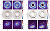 |
Fig. A.1. Lens modelling results of the two lenses: B1938+666 in the K′ Keck band (left) and J0946+1006 in the F814W band (right). For each lens, we present the result of the smooth model and the model that includes the NFW profile with free concentration. In each case, we show (i) the best-reconstructed model and critical lines, including both the light of the central galaxy and the main arc, (ii) the residuals between the data and the best model, calculated as (data-model) and (iii) the corresponding best-reconstructed source with the caustics. The posterior distributions for all models are shown in Fig. A.4 and A.5. |
 |
Fig. A.2. We zoom on the detection location in J0946+1006 and show the residuals between the model and the data for all considered variations of subhalo properties. In each panel, the dashed blue line shows the critical curve predicted by the model, and the black contours trace the surface brightness of the arc. In the first panel, we see a clear red spot at the edge of the lensed arc, which is close to the detection location and indicates that the smooth model cannot correctly reproduce the surface brightness distribution. The NFW models with fixed concentration (second panel) and position (third panel) cannot remove this excess, while the residuals reach the noise level when the NFW is allowed to have a higher concentration (fourth panel) or when we use a PJ or PL profile (last two panels). |
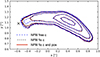 |
Fig. A.3. Contours showing the surface brightness distribution of the lensed arc of J0946+1006 when modelled with the inclusion of an NFW profile. The three cases shown here correspond to panel 1-4 in Fig. A.2 and highlight that, among these, only the NFW model with free concentration (dashed blue line) is able to produce the extended shape of the arc's edge which matches the surface brightness of the observes arc. |
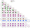 |
Fig. A.4. Full posterior distributions for the system B1938+666, including the parameters describing the lens, source regularisation and subhalo. We show the smooth model (gree) and the perturbed models that include a subhalo described as PJ, PL or NFW with free concentration. |
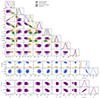 |
Fig. A.5. Full posterior distributions for the system J0946+1006. |
Appendix B: Subhalo Mass Bias and additional scaling relations
Here we compare the subhalo masses obtained by integrating the best modified NFW profile fits with the masses obtained by summing up the individual masses of all the particles in the simulation that are bound to the subhalo.
The top panels of Fig. B.1 illustrate the results of this analysis. In the left panel, the subhalo masses obtained by integrating the best modified NFW profile are plotted against those obtained from the particle data for all the subhaloes in the TNG50 sample. Here, one can already see that the modified NFW profile can accurately reproduce the actual subhalo masses with only small errors. Overall, the modified NFW profile is biased in the sense that the inferred masses are, on average, underestimated. This is especially true for subhaloes with Msub≥1011 M⊙, where the most likely cause for the underestimation is the fact that the central bumps with an increased density are not parametrised by the model.
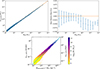 |
Fig. B.1. Top−left: the subhalo masses obtained by integrating the best modified NFW profile fits are plotted against the subhalo masses obtained from the particle data of the TNG50 simulation. The dashed orange line indicates where both masses are equal. Top−right: the mean relative errors of the subhalo masses obtained by integrating the best modified NFW profile fits are plotted against the true subhalo masses obtained from the simulation data for each mass bin. The standard deviations are indicated by the error bars. Bottom: Scaling of the Einstein radius (obtained by using the best modified NFW profile fits) with |

For 79.4 per cent of the subhaloes, the deviation from the true mass is less than 5 per cent, and for 26.3 per cent of the subhaloes, the deviation is less than 1 per cent. The right panel shows in more detail how much the masses are underestimated in each mass bin. One can see that the best mass estimates are obtained for subhaloes with masses in the range 109 M⊙ ≤Msub≤1010 M⊙, which is close to the range in which the modified NFW profile provides the best fits for the individual and average subhalo density profiles.
In Sect. 5.3, we calculated linear scaling relations between the Einstein radius Rein, the subhalo mass and circular velocity. Another relation with a small scatter can be found when looking at how the Einstein radius obtained from the best mNFW profile fit Rein,mNFW scales with  (see the bottom panel of Fig. B.1). The best power law fit for this relation is given by:
The existence of this scaling relation can be easily explained using a scaling relation for the rs parameter of the modified NFW profile from Heinze et al. (2024):
According to this equation, dividing the subhalo mass by rs leads to the approximate cancellation of Msub and  is left. This results in the scaling we find in the Rein,mNFW−Vmax relation in Equation (13) and therefore the exponent in Equation (14) is approximately equal to 1.
All Tables
Summary of most relevant works in which the two systems considered here have been modelled – with or without the perturber.
All Figures
|
Fig. 1. Images of the two strong gravitational lensing systems used in this paper, where subhalo detections (marked by a white cross) have been claimed in previous works. Left: image of B1938+666 taken in the K′ band by NIRC2 on Keck. In this case, zL = 0.881 and zs = 2.059; the pixel and FWHM (determining the resolution) scales are 10 and 70 milli-arcseconds (hereafter, mas), respectively. Right: HST F814W observations of the lens J0946+1006. For this system, zL = 0.222 and zs = 0.609; the pixel size and resolution are 50 and 90 mas, respectively. See Table 1 for a list of previous analyses of these systems. |
| In the text | |
|
Fig. 2. Left: nested sampling posterior distributions for parameters describing the subhalo in the system B1938+666 for the PJ (orange) and NFW (blue and gray) profiles. In all cases, we fit for the subhalo mass Msub (in M⊙) and position (xsub and ysub, measured in arcseconds with respect to the centre of the image). We also plot the posterior of the subhalo position of the PL profile (purple), while the other parameters describing the models are plotted separately in Fig. 4. We consider two variations of the NFW profile: one (grey) where the concentration csub is fixed by the concentration–mass relation from Duffy et al. (2008) and a case (blue) where csub is left free to vary. The best-fit values derived from the posteriors are listed in Table 2. Note that we plot the mass Msub in logarithmic space for better comparing the model, and this may give the impression that the grey contours are reaching the edge of the prior, which is not the case. The black rectangle in the (xsub−ysub) panel indicates the pixel scale of the data. The best lens model and reconstructed source for the smooth and smooth+NFW cases are shown in the Appendix in Figs. A.1 and A.4 shows the posterior distribution for all parameters in all considered models. Right: radial density and projected enclosed mass profiles corresponding to the best-fit subhalo profiles in the left panel, i.e. to the values reported in Table 2 (mean and 95 CL). The profiles are calculated analytically following the definitions in Sect. 2.2. The vertical dashed lines in the top panel mark the slope transition for the NFW and PJ profiles, i.e. rs and rt. In the bottom panel, the dotted lines mark the distance at which the PJ, NFW and PL curves intersect, thus predicting the same mass, i.e. req = 0.9 kpc. The grey areas show the data resolution. |
| In the text | |
|
Fig. 3. Same as Fig. 2 but for the lens system J0946+1006. Here, the NFW profile with concentration fixed by the concentration–mass relation is a worse fit to the data than the other models: a symptom is the best-fit position of the subhalo, which is very different and more uncertain than for the other profiles. Moreover, the enclosed mass in the bottom-right panel does not converge within a radius similar to the other two profiles, i.e. Req = 0.45 kpc. The best models and the full posterior distributions can be found in the appendix in Figs. A.1 and A.5. |
| In the text | |
|
Fig. 4. Posterior distribution of the PL model parameters: the slope, γsub, and the convergence normalisation, log(κsub), measured in arcseconds. The dashed lines mark the slope of an isothermal profile. |
| In the text | |
|
Fig. 5. Comparison of the NFW models from our analysis (black circles and blue squares) and previous works with concentration–mass–redshift relations derived from N-body simulations. All results are expressed in terms of the virial mass of haloes Mvir, except for Moliné et al. (2017) who measured the relation using M200, i.e. the mass within the radius enclosing an overdensity of 200. In this case, the relation has an additional dependence on the distance of the subhalo from the centre of its host halo. Since the observational results are derived in projection (on the lens plane), we cannot determine the three-dimensional distance from the host centre, and we plot a range of relations for distances between 0.1Rvir and Rvir. Given that it was calibrated on subhaloes rather than isolated haloes, it naturally predicts higher concentrations at the low-mass end. In each panel, the coloured symbols and error bars show our inferred values from the analysis of the observations (black circle and blue square) and the results from previous works (empty symbols), listed in Table 2. Şengül & Dvorkin (2022) used a fixed mass Msub = 109 M⊙ and varied the inner slope of the profile (that we report in the table), from which they estimated a corresponding concentration but did not provide uncertainties in this quantity. |
| In the text | |
|
Fig. 6. Zoom on the location of the two detections to highlight the differences in the critical lines and subhalo position between the considered models (lines and crosses of the corresponding colour). The circles marks (i) the radius, Req, at which the PJ and NFW profiles produce the same enclosed mass (solid white), (ii) the Einstein radius, Rein, calculated with Equation (3) for the PL profile (purple), (iii) the size corresponding to the robust mass defined for J0946+1006 by Minor et al. (2021, dashed white). In the case of B1938+666, the perturber is very compact, and the three best models have very similar critical lines. In J0946+1006, the larger subhalo mass translates into larger visible differences among the models. |
| In the text | |
|
Fig. 7. Comparison between the γsub inferred from observations with the PL model (see Fig. 4) and the inner slopes of subhaloes from the TNG50-1 simulation. In the latter, the slope has been measured for all subhaloes in H23 (see their Fig. 9). The bottom panel shows the distribution of slopes of all subhaloes (black) and two mass bins roughly corresponding to the range of the detections. The coloured vertical lines and shaded areas correspond to the observed values (Table 2). In the top panel, we show the cumulative distribution for all subhaloes and the second mass bin, and we report the corresponding fractions of subhaloes that are compatible with the observed slopes in the two mass bins, highlighting the one that better corresponds to the detection in each case with the horizontal lines and corresponding numbers. |
| In the text | |
|
Fig. 8. Top: log-slope of the surface density profile around r=Req = 0.9 kpc (for B1938+666) or r = 1 kpc (for J0946+1006) against the projected total mass enclosed within the same distance. See Fig. 13 for the J0946+1006 results at r=Req, which we believe are affected by resolution. The coloured points indicate the top 10 percent of lines of sight that yielded the largest density values, colour-coded by the stellar-to-total mass ratio. The grey dots indicate the averages over all 1000 lines of sight. The larger points show the slope and mass values inferred from our lens modelling for the PJ (orange circle), NFW with free concentration (blue diamond) and PL (pink square) profiles. In the right panel, we also compare to the measurement by Minor et al. (2021). Bottom: total subhalo mass as a function of the enclosed projected mass. Points are coloured by the total stellar mass of the subhalo. The mean and standard deviation used in Equation (11) are represented by the solid and dotted black lines. |
| In the text | |
|
Fig. 9. Comparison of the luminosity of the simulated subhaloes and the observational limits set for the two detections. First, we selected the systems that best match the observational inference in terms of projected slope and enclosed mass: in practice, these were selected within the orange rectangles in the top panels of Fig. 8. We computed their luminosity, LV, from the V-band magnitudes provided in the TNG50-1 subhalo catalogue and plot them as orange circles as a function of the subhalo mass, Msub. We show the results for B1938+666 on the left and J0946+1006 on the right. The black dots show instead the luminosity of the general subhalo population at the same redshift. The observational upper limits (see Sect. 3) are represented by the horizontal red line in the plot. |
| In the text | |
|
Fig. 10. Subhalo density profiles of the simulated subhaloes that best match the observational inference (B1938+666 on the left and J0946+1006 on the right), i.e. the same shown in orange in Fig. 9. The purple band shows the radial range used to measure the slope, γ2D, for Fig. 8. The vertical lines mark the softening of the simulation (vertical solid line), and the value commonly used in simulation as a reliable resolution limit (i.e. 2.3ϵDM,*, vertical dashed line) and the resolution of the observational data. |
| In the text | |
|
Fig. 11. Properties of simulated subhaloes at infall. We used the merger trees to track the subhalo evolution and measure their properties at infall, i.e. at the redshift where they first entered their host halo. We plot the normalised distribution of infall redshifts zinfall (left) and the mass at infall Minfall (right). The orange histograms show the distribution of the subhaloes selected as analogues, i.e. those lying within the orange boxes in the top panels of Fig. 8 for which we show the density profiles in the bottom panels of the same figure. The grey histograms show instead the distribution for all subhaloes in the same host haloes and with final masses between 2×10⁸ M⊙≤Msub(z = 0.89)≤5×10⁹ M⊙ for B1938+666 and 109 M⊙≤Msub(z = 0.2)≤4×10¹¹ M⊙ for J0946+1006. |
| In the text | |
|
Fig. 12. Scaling of the Einstein radius (obtained from the best mNFW fits) with subhalo mass (left) and Vmax (right). In both plots, the colour-coding of the data points indicates the subhalo stellar mass M*. The cyan lines represent the best power law fit for all of the data points. |
| In the text | |
|
Fig. 13. Tests of the impact of numerical resolution on our results. Left and central panel: comparison between the Einstein radii obtained from the best modified NFW profile fits (in grey – corresponding to the points in Fig. 12) and those calculated from the smoothed particle surface density maps, coloured by the subhalo stellar mass. The cyan lines are the best power law fits for the latter. In both plots, the regime below the softening length is coloured purple. Right: repeat of the measurements performed for Fig. 8, using Req = 0.45 kpc for the lens J0946+1006. |
| In the text | |
|
Fig. A.1. Lens modelling results of the two lenses: B1938+666 in the K′ Keck band (left) and J0946+1006 in the F814W band (right). For each lens, we present the result of the smooth model and the model that includes the NFW profile with free concentration. In each case, we show (i) the best-reconstructed model and critical lines, including both the light of the central galaxy and the main arc, (ii) the residuals between the data and the best model, calculated as (data-model) and (iii) the corresponding best-reconstructed source with the caustics. The posterior distributions for all models are shown in Fig. A.4 and A.5. |
| In the text | |
|
Fig. A.2. We zoom on the detection location in J0946+1006 and show the residuals between the model and the data for all considered variations of subhalo properties. In each panel, the dashed blue line shows the critical curve predicted by the model, and the black contours trace the surface brightness of the arc. In the first panel, we see a clear red spot at the edge of the lensed arc, which is close to the detection location and indicates that the smooth model cannot correctly reproduce the surface brightness distribution. The NFW models with fixed concentration (second panel) and position (third panel) cannot remove this excess, while the residuals reach the noise level when the NFW is allowed to have a higher concentration (fourth panel) or when we use a PJ or PL profile (last two panels). |
| In the text | |
|
Fig. A.3. Contours showing the surface brightness distribution of the lensed arc of J0946+1006 when modelled with the inclusion of an NFW profile. The three cases shown here correspond to panel 1-4 in Fig. A.2 and highlight that, among these, only the NFW model with free concentration (dashed blue line) is able to produce the extended shape of the arc's edge which matches the surface brightness of the observes arc. |
| In the text | |
|
Fig. A.4. Full posterior distributions for the system B1938+666, including the parameters describing the lens, source regularisation and subhalo. We show the smooth model (gree) and the perturbed models that include a subhalo described as PJ, PL or NFW with free concentration. |
| In the text | |
|
Fig. A.5. Full posterior distributions for the system J0946+1006. |
| In the text | |
|
Fig. B.1. Top−left: the subhalo masses obtained by integrating the best modified NFW profile fits are plotted against the subhalo masses obtained from the particle data of the TNG50 simulation. The dashed orange line indicates where both masses are equal. Top−right: the mean relative errors of the subhalo masses obtained by integrating the best modified NFW profile fits are plotted against the true subhalo masses obtained from the simulation data for each mass bin. The standard deviations are indicated by the error bars. Bottom: Scaling of the Einstein radius (obtained by using the best modified NFW profile fits) with |
| In the text | |
Current usage metrics show cumulative count of Article Views (full-text article views including HTML views, PDF and ePub downloads, according to the available data) and Abstracts Views on Vision4Press platform.
Data correspond to usage on the plateform after 2015. The current usage metrics is available 48-96 hours after online publication and is updated daily on week days.
Initial download of the metrics may take a while.