| Issue |
A&A
Volume 698, May 2025
|
|
|---|---|---|
| Article Number | A7 | |
| Number of page(s) | 27 | |
| Section | Galactic structure, stellar clusters and populations | |
| DOI | https://doi.org/10.1051/0004-6361/202553673 | |
| Published online | 23 May 2025 | |
LAMOST medium-resolution observations of the Pleiades
1
INAF – Osservatorio Astrofisico di Catania,
via S. Sofia, 78,
95123
Catania,
Italy
2
Institute for Frontiers in Astronomy and Astrophysics, Beijing Normal University,
Beijing
102206,
PR
China
3
School of Physics and Astronomy, Beijing Normal University,
Beijing
100875,
PR
China
4
University of Wrocław, Faculty of Physics and Astronomy, Astronomical Institute,
ul. Kopernika 11,
51-622
Wrocław,
Poland
5
Royal observatory of Belgium,
Ringlaan 3,
1180
Brussel,
Belgium
★ Corresponding author: antonio.frasca@inaf.it
Received:
3
January
2025
Accepted:
7
April
2025
Aims. In this work, we present the results of our analysis of medium-resolution LAMOST spectra of late-type candidate members of the Pleiades with the aim of determining the stellar parameters, activity level, and lithium abundance.
Methods. We used the ROTFIT code to determine the atmospheric parameters (Teff, log g, and [Fe/H]), along with the radial velocity (RV) and projected rotation velocity (v sin i). Moreover, for late-type stars (Teff ≤ 6500 K), we also calculated the Hα and Li Iλ6708 net equivalent width by means of the subtraction of inactive photospheric templates. We also used the rotation periods from the literature and we purposely determined them for 89 stars by analyzing the available Transiting Exoplanet Survey Satellite (TESS) photometry.
Results. We derived the RV, v sin i, and atmospheric parameters for 1581 spectra of 283 stars. Literature data were used to assess the accuracy of the derived parameters. The RV distribution of the cluster members peaks at 5.0 km s−1 with a dispersion of 1.4 km s−1, while the average metallicity is [Fe/H]=−0.03±0.06, in line with previous determinations. Fitting empirical isochrones of Li depletion to EW measures of stars with Teff ≤ 6500 K, we obtained a reliable age for the Pleiades of 118±6 Myr, in agreement with the recent literature. The activity indicators Hα line flux (FHα) and luminosity ratio (R′Hα) show the hottest stars to be less active (on average) than the coldest ones, as expected for a 100-Myr old cluster. When plotted against the Rossby number, RO, our R′Hα values display a typical activity-rotation trend, with a steep decay for RO ≥ 0.2 and a nearly flat (saturated) activity level for smaller values. However, we still see a slight dependence on RO in the saturated regime, which is well fitted by a power law with a slope of −1.18 ± 0.02; this is in agreement with a number of previous works. For three sources with multi-epoch data, we had access to LAMOST spectra acquired during flares, which are characterized by strong and broad Hα profiles and the presence of the He I λ6678 Å emission line. Among our targets, we identified 39 possible SB1 and ten SB2 systems. We have also shown the potential of the LAMOST-MRS spectra in allowing us to refine the orbital solution of a number of binaries and to discover a new double-lined binary as well.
Key words: stars: abundances / stars: activity / binaries: spectroscopic / stars: flare / stars: fundamental parameters / open clusters and associations: individual: Pleiades
© The Authors 2025
 Open Access article, published by EDP Sciences, under the terms of the Creative Commons Attribution License (https://creativecommons.org/licenses/by/4.0), which permits unrestricted use, distribution, and reproduction in any medium, provided the original work is properly cited.
This article is published in open access under the Subscribe to Open model. Subscribe to A&A to support open access publication.
1 Introduction
Open clusters (OCs) result from the gravitational collapse of molecular clouds. After the gas dispersal occurring in the first ≈100 Myr, stellar populations with homogeneous ages and chemical compositions are left behind (see Krumholz et al. 2019, for a recent review). Over the course of their evolution, stars belonging to open clusters are gradually dispersed within the Galaxy by tidal disruption and N-body evaporation, becoming field stars. Therefore, OCs can be considered as the building blocks of our and other galaxies. Members of OCs that are bound by mutual gravitation provide ideal samples for studying stellar properties such as rotation and magnetic activity as a function of the stellar mass, unaffected by variations in age or metallicity (e.g., Barnes 2003; Fang et al. 2018; Frasca et al. 2015). Young OCs, particularly those of ≈100 Myr, have already removed most of the gas and recently stabilized in nuclear fusion processes, making them excellent candidates for these studies.
Among the OCs of the Milky Way, the Pleiades hold a unique position, serving as an ideal laboratory for investigating stellar evolution. Its proximity to Earth (≈130 pc) and the estimated age of 125 Myr, based on the lithium depletion boundary (Basri et al. 1996; Stauffer et al. 1998), make it the closest young OC and a prototype for studying young solar-type stars in cluster environments. In this regard, the works of Soderblom et al. (1993a,b), based on the analysis of high-resolution spectra of a relevant number of members, are of fundamental importance for the study of the rotation, activity, and abundance of lithium.
Research on the Pleiades cluster over the past few decades has advanced our understanding of the relationships between stellar rotation, magnetic activity, and radius inflation. Early studies identified correlations between radius inflation and magnetic activity (e.g., Torres et al. 2006; López-Morales 2007; Morales et al. 2008; Stassun et al. 2012), which was further investigated using theoretical models (e.g., Feiden & Chaboyer 2013, 2014; Jackson & Jeffries 2014a,b; Somers & Pinsonneault 2014, 2015a,b). Barrado et al. (2016) found a strong connection between lithium depletion, rotation, and activity in Pleiades F, G, and K stars, particularly for stars with luminosities in the range of 0.5–0.2 L⊙. Cao & Pinsonneault (2022) measured starspot filling fractions for 240 stars in the Pleiades, showing that active stars reach a saturation level of 0.248 ± 0.005, with slower rotators showing a decline. These theoretical insights set the foundation for future observational studies. For example, Somers & Stassun (2017) employed a fitting of the spectral energy distribution to confirm the magnetic origin of the radius inflation in the Pleiades by analyzing 83 stars, demonstrating a clear connection between rapid rotation, magnetic activity, and enhanced lithium abundance. Building on this, Jackson et al. (2018) used maximum-likelihood modeling to investigate the inflated radii of low-mass stars in the Pleiades, highlighting the roles of magnetic inhibition of convection and stellar spots in driving radius inflation, in comparison with earlier findings by Rebull et al. (2016).
More recent research has expanded on these foundational studies by incorporating new data and methodologies. Wanderley et al. (2024) analyzed APOGEE spectra to measure the magnetic fields of 62 M-type dwarfs in the Pleiades, revealing a strong correlation between magnetic field strength, rotation, and radius inflation. Other investigations have broadened the focus to stellar properties and dynamics. For instance, Heyl et al. (2022) utilized Gaia EDR3 data to identify 289 stars that have escaped the cluster, including three white dwarfs, providing insights into the cluster’s dynamical evolution. Additionally, Alfonso & García-Varela (2023) identified 958 cluster members using Gaia DR3 data (Gaia Collaboration 2023), confirming the consistency of the cluster’s distance, age, and metallicity with previous studies (Gaia Collaboration 2018; Bossini et al. 2019). These efforts, along with studies on lithium-rotation correlations (Bouvier et al. 2018), spot activity (Fang et al. 2016), and the influence of cool starspots on stellar evolution (Guo et al. 2018), continue to deepen our understanding of stellar evolution in young OCs.
The Large Sky Area Multi-Object Fiber Spectroscopic Telescope (LAMOST; Cui et al. 2012) is a National Major Scientific Project undertaken by the Chinese Academy of Science. It is a unique instrument, located at the Xinglong station and situated south of the main peak of the Yanshan mountains in Hebei province (China). LAMOST combines a large aperture (4-meter telescope) with a wide field of view (circular region with a diameter of 5 degrees on the sky) that is covered by 4000 optical fibers. These fibers are connected to 16 multi-object optical spectrometers with 250 fibers each (Wang et al. 1996; Xing et al. 1998), making this instrument the ideal tool for obtaining spectroscopic observations for a large number of targets in an efficient way. The data acquired with the LAMOST instrument allow for multi-fold analyses of the observed objects to be conducted, including a homogeneous determination of the atmospheric parameters (APs): the effective temperature, Teff, surface gravity, log g, metallicity, [Fe/H], as well as the radial velocity, RV, and projected rotational velocity, v sin i. Leveraging unique LAMOST medium-resolution spectroscopic data, this study aims to address critical questions about stellar activity, rotation, and lithium abundance in young stars.
This paper is organized as follows. Section 2 presents the selection of the targets that make up our sample and the photometric and spectroscopic data used in this work. In Sect. 3, we describe the data analysis performed with the code ROTFIT. We also discuss the data quality by comparing our results with values from the literature. Section 4 concerns the rotation periods used in this work, part of which we derived by analyzing light curves acquired by NASA’s Transiting Exoplanet Survey Satellite (TESS). In Sect. 5, we introduce the procedure for measuring activity indicators and lithium abundance. Section 6 shows the multi-epoch monitoring of some stars, thanks to which remarkable flares events were detected for a few sources. The age of the cluster is discussed in detail in Sect. 7. The analysis of RV curves for some spectroscopic binaries present in our sample is carried out in Sect. 8. We provide a summary of our findings in Sect. 9.
2 Observations and sample selection
2.1 Sample selection
The first step of our study is the selection of bona-fide members of the Pleiades. To this aim, we have used the list of 1061 members selected by Cantat-Gaudin et al. (2018) on the basis of their astrometric and photometric properties. They applied an unsupervised membership assignment code (UPMASK) to the Gaia DR2 data down to G = 18 mag in the fields of a large number of OCs, including the Pleiades. Another important source of information for our study was the new catalog of members of galactic OCs compiled by Hunt & Reffert (2024), who used a similar approach, but with a different algorithm applied to the Gaia DR3 data down to magnitude G ≈ 20 mag. They found 1721 Pleiades members, 1042 of which are in common with Cantat-Gaudin et al. (2018). The higher number of sources in Hunt & Reffert (2024), apart from the different algorithm, is mostly the result of a larger sampled sky area and the deeper limiting magnitude. Their cluster membership lists include many new members of the already known clusters and often encompass tidal tails, as is likely the case of the Pleiades (e.g., Dinnbier & Kroupa 2020). Another important source of information is the list of the 759 Pleiades members observed with Kepler-K2 space mission for which Rebull et al. (2016) reported periods and variation amplitudes. Many of these stars (548) are also members according to Cantat-Gaudin et al. (2018) and 709 are in the Hunt & Reffert (2024) catalog. Due to the different selection criteria adopted by Rebull et al. (2016), further 50 sources are not included in any of the previous catalogs. We compiled a final list of 1790 likely members selected from at least one of the aforementioned catalogs, which is the result of adding the 19 Cantat-Gaudin et al. (2018) members not included in the previous catalog and the 50 Rebull et al. (2016) additional sources not contained in either of the two previous lists to the 1721 members of Hunt & Reffert (2024). Figure 1 shows the spatial distribution, the position on the color-magnitude diagram (CMD), and the proper motion diagram. We used different symbols to designate the stars classified in different papers as members of the Pleiades. We remark that we updated the photometric and kinematic data of the investigated sources with the Gaia DR3 in this figure and in the rest of the paper. We note a handful of candidate members that lie far below the cluster sequence in the CMD. However, as shown by the red dots, none of them have been observed with LAMOST-MRS, while some members lie just above the main sequence (MS), but close to the binary sequence. Regarding their kinematic properties, almost all stars observed with LAMOST-MRS fall within the 3σ ellipse of the proper motion (PPM) distributions defined by Hunt & Reffert (2024) or just outside it. The largest scatter in the PPM diagram is shown by some members of Hunt & Reffert (2024) that outline a tail-like structure and by the few candidates of Rebull et al. (2016) that are not included in the other two lists. The latter sources can be considered low-probability members or probable contaminants. However, very few of them (≈10) have been observed with LAMOST-MRS and are included in our analysis.
2.2 Spectroscopy
LAMOST started a five-year medium-resolution spectroscopic survey (MRS, R ~ 7500, 4950 Å < λ < 5350 Å (blue arm) and 6300 Å < λ < 6800 Å (red arm); Liu et al. 2020) in 2017 September, after a five-year low-resolution spectroscopic survey (LRS; R ~ 1800, 3800 Å < λ < 9000 Å). Each arm of each of the 16 spectrographs uses a 4K×4K EEV CCD with 12 μm square pixels as a detector. In the blue arm, the CCD pixel size corresponds to a sampling Δλ ≃ 0.12 Å, while in the red arm, it corresponds to about 0.15 Å (Cui et al. 2012; Wang et al. 2019). LAMOST MRS DR11, which we use in this paper, contains the data obtained from 2017 September to 2023 June (about 46 million spectra) and is currently available to the Chinese astronomical community only. The APs resulting from the automatic analysis of the raw spectra with the LASP pipeline (Luo et al. 2015; Wang et al. 2019), implemented specifically for LAMOST, are given in the LAMOST MRS Parameter Catalog of DR111.
The cross-match of the Cantat-Gaudin et al. (2018) sample with the LAMOST DR11 catalog, adopting a radius of ![$\[3^{\prime\prime}_\cdot7\]$](/articles/aa/full_html/2025/06/aa53673-25/aa53673-25-eq3.png) on the basis of the fiber pointing precision
on the basis of the fiber pointing precision ![$\[0^{\prime\prime}_\cdot4\]$](/articles/aa/full_html/2025/06/aa53673-25/aa53673-25-eq4.png) and the
and the ![$\[3^{\prime\prime}_\cdot3\]$](/articles/aa/full_html/2025/06/aa53673-25/aa53673-25-eq5.png) diameter of the fiber (e.g., Zong et al. 2018), produced 260 targets with MRS spectra, all in common with Hunt & Reffert (2024), 233 of which have spectra with a sufficient signal-to-noise ratio per pixel in at least one arm (S/N≥5) to be worthy of analysis. None of the 19 Pleiades members according to Cantat-Gaudin et al. (2018) but not recovered by Hunt & Reffert (2024) was observed by LAMOST MRS. A further 37 Hunt & Reffert (2024) members have LAMOST MRS data of sufficient quality. Among the additional 50 Rebull et al. (2016) members, 15 were observed with LAMOST MRS and the spectra of 13 of them had a high-enough S/N to be analyzed with our tools. We also considered them in our analysis, which is therefore based on a total sample of 283 Pleiades members or candidates (highlighted with red dots in Fig. 1). Due to the different selection criteria, we also investigated possible differences between these three subsamples, which are henceforth referred to as Cantat, Hunt, and Rebull. In total, we collected 1581 LAMOST MRS co-added spectra that correspond to 283 different stars among our list of likely members of the Pleiades. We preferred to use co-added spectra, where each spectrum is the sum of all exposures obtained in a single observing night, to have the best possible S/N. Some objects were even observed in as many as 14 different epochs.
diameter of the fiber (e.g., Zong et al. 2018), produced 260 targets with MRS spectra, all in common with Hunt & Reffert (2024), 233 of which have spectra with a sufficient signal-to-noise ratio per pixel in at least one arm (S/N≥5) to be worthy of analysis. None of the 19 Pleiades members according to Cantat-Gaudin et al. (2018) but not recovered by Hunt & Reffert (2024) was observed by LAMOST MRS. A further 37 Hunt & Reffert (2024) members have LAMOST MRS data of sufficient quality. Among the additional 50 Rebull et al. (2016) members, 15 were observed with LAMOST MRS and the spectra of 13 of them had a high-enough S/N to be analyzed with our tools. We also considered them in our analysis, which is therefore based on a total sample of 283 Pleiades members or candidates (highlighted with red dots in Fig. 1). Due to the different selection criteria, we also investigated possible differences between these three subsamples, which are henceforth referred to as Cantat, Hunt, and Rebull. In total, we collected 1581 LAMOST MRS co-added spectra that correspond to 283 different stars among our list of likely members of the Pleiades. We preferred to use co-added spectra, where each spectrum is the sum of all exposures obtained in a single observing night, to have the best possible S/N. Some objects were even observed in as many as 14 different epochs.
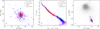 |
Fig. 1 Left panel: spatial distribution of the Pleiades members according to Hunt & Reffert (2024, purple dots) and Cantat-Gaudin et al. (2018, blue dots). The symbol size scales with the G magnitude. The green diamonds mark the K2 variable stars in Rebull et al. (2016) that are not members according to either Hunt & Reffert (2024) or Cantat-Gaudin et al. (2018). Red dots represent the stars observed with LAMOST MRS. The meaning of the symbols is also indicated in the legend. Middle panel: color–magnitude diagram of the same sources. Right panel: proper motion diagram of all the Gaia DR3 sources with G ≤ 15 mag (small grey dots) in the field of the Pleiades (center coordinates RA(2000) = 03h46m, Dec(2000) = +24°06′, radius 4°). The Pleiades members are highlighted with the same symbols as in the other panels. The cyan asterisk denotes the average proper motion of the cluster according to Hunt & Reffert (2024) and the cyan ellipse is the 3σ contour. |
2.3 Photometry
Space-born precise photometry for many targets was collected by the Kepler-K2 mission. For most of these sources the rotational periods, Prot, were derived by Rebull et al. (2016). For the stars without Prot values in this catalog, we have analyzed space-based photometry collected with TESS (Ricker et al. 2015). Our targets were mostly observed by TESS in three consecutive sectors, namely 42 (from 2021-08-20 to 2021-09-16), 43 (from 2021-09-16 to 2021-10-12), and 44 (from 2021-10-12 to 2021-11-06). The observations in these three consecutive sectors allowed us to obtain nearly uninterrupted sequences (with only a few gaps of ≈ 1 day) of high-precision photometry lasting about 77 days, with a cadence of two minutes. For a sparse and nearby cluster such as the Pleiades, there is no severe star crowding, also taken the large pixel size of TESS (21″) into account. Therefore, for most sources, we do not expect a relevant flux contamination from nearby sources. In any case, we did not consider the data for members with a companion with a comparable (or lower) magnitude within 30″. We downloaded the TESS light curves reduced by the MIT Quick Look Pipeline (QLP, Huang et al. 2020) from the MAST2 archive and used the simple aperture photometry flux (SAP).
3 Data analysis
We applied the code ROTFIT (e.g., Frasca et al. 2006, 2015) to measure the RV, v sin i, and the APs (Teff, log g, and [Fe/H]). We adapted the code to fit with the LAMOST MRS, as we had already done in a previous work (Frasca et al. 2022) analyzing thousands of MRS spectra in the Kepler field. The grid of templates consisted of high-resolution spectra of slowly rotating stars (v sin i ≤ 3 km s−1) with a low activity level, retrieved from the ELODIE archive (R≃42 000; Moultaka et al. 2004). This is the same grid that is used in Frasca et al. (2022) and for the analysis of young stars within the Gaia-ESO survey by the OACT (Osservatorio Astrofisico di Catania) node (Frasca et al. 2015). It contains the spectra of 388 different stars, which sufficiently cover the space of the APs, especially at metallicity values near the solar ones, which are typical for the young OCs. We preferred to use real star spectra over synthetic ones because the former reproduce the photospheric features better than the latter, whereby some lines may be missing or poorly reproduced due to uncertain values of strength, Landé factors, and broadening coefficients for the corresponding transitions. Moreover, the subtraction of the nonactive photospheric template from the target spectrum is of great help because it leaves as residuals the chromospheric core contribution and the Li I line cleaned from blended neighbor lines.
The analysis steps can be summarized as: (i) normalization of LAMOST spectra (both the blue- and red-arm) by a fit of a low-order polynomial; (ii) measurement of the RV by the cross-correlation with a few templates chosen from the ELODIE grid; (iii) determination of the APs and v sin i by χ2 minimization of the residuals of the differences observed–templates, with each template being rotationally broadened by the convolution with a linear-limb-darkened rotational profile of varying v sin i3; (iv) spectral type (SpT) classification by taking that of the template with the minimum χ2; and v) measurement of the equivalent width of the emission in the Hα core and residual absorption in the Li I λ6708 line in the subtracted spectra. For the details about the procedure, we refer to Frasca et al. (2022).
For the stars with more than one LAMOST-MRS spectrum we have computed, for each arm, the APs for the three best exposed spectra and averaged them using a variance-defined weight ![$\[w_{i}=1 / \sigma_{i}^{2}\]$](/articles/aa/full_html/2025/06/aa53673-25/aa53673-25-eq6.png) , where σi is the error of the given parameter in the i-th measure. Therefore, we ended up with only two values of Teff, log g, [Fe/H], and v sin i per each target, one derived from the analysis of the blue-arm and the other of the red-arm spectra. The final parameters (reported in Table 1) are the weighted mean of the values derived from each arm, using again the variance-defined weights. Whenever the APs could only be measured in one arm (usually in the red arm) due to the low S/N or flaws in the spectrum of the other arm, we have taken these values as the final ones. The parameter errors calculated by ROTFIT or the standard errors of the weighted mean, for the sources with multiple observations, are also quoted in this table.
, where σi is the error of the given parameter in the i-th measure. Therefore, we ended up with only two values of Teff, log g, [Fe/H], and v sin i per each target, one derived from the analysis of the blue-arm and the other of the red-arm spectra. The final parameters (reported in Table 1) are the weighted mean of the values derived from each arm, using again the variance-defined weights. Whenever the APs could only be measured in one arm (usually in the red arm) due to the low S/N or flaws in the spectrum of the other arm, we have taken these values as the final ones. The parameter errors calculated by ROTFIT or the standard errors of the weighted mean, for the sources with multiple observations, are also quoted in this table.
Stellar parameters of the investigated sources.
Radial velocity standard stars in the fields of LAMOST observations used in this paper.
3.1 Radial velocity
As noted by Zong et al. (2020) and Frasca et al. (2022), the RV measured on LAMOST–MRS spectra can be affected by systematic offsets in different runs that are related to the wavelength calibration and can be different for the blue and red arm. The largest offset of about 6.5 km s−1 is found for spectra acquired before May 2018 that were calibrated with Sc lamps, compared to the following ones for which Th–Ar lamps have been used. To account for these offsets and correct the RVs, we have used the spectra of RV standard stars from Soubiran et al. (2018) and Huang et al. (2018) falling in the same plates as those of our Pleiades candidates and taken at the same time (see Table 2). For a few plates, we found only one or no standard star. In these cases, we used the RVs of stars with G ≤ 12 mag in the Gaia-DR3 catalog with an RV error ≤0.5 km s−1 as reference, similar to what was done in the study by Zong et al. (2020). Although they are not RV standard stars in the strict sense, the use of a statistically significant number of them ensures a good determination of the RV offset. Indeed, we found a good agreement between the offset calculated with the RV standard stars listed in Table 2 and those with RVs from Gaia. We applied the proper corrections to the blue- and red-arm RVs. The RV corrections for each plate and observing date are reported (for the blue- and red-arm spectra) in Table A.1.
An indicator of the precision of the RV measures that has been used in Frasca et al. (2022) is provided by the comparison of the blue- and red-arm results. In Fig. 2, we compare the RV values obtained with the two arms, whose observations are done simultaneously, for all the spectra of the Pleiades members with an S/N ≥ 10. This suggests an independent error estimate of about 2.2 km s−1, which was derived by dividing the dispersion of the differences ΔRV = RVblue − RVred = 3.1 km s−1 by ![$\[\sqrt{2}\]$](/articles/aa/full_html/2025/06/aa53673-25/aa53673-25-eq7.png) . The rms dispersion is slightly larger than that found by Frasca et al. (2022) for a larger sample of MRS spectra in the Kepler field; this could be due to the quality of the spectra of the Pleiades members, which have a median S/N = 74 and 32 in the red and blue arm, respectively. For comparison, the spectra of the LAMOST–Kepler sample analyzed by Frasca et al. (2022) had a median S/N of 91 and 52 in the red and blue arm, respectively. The errors we find in the present work are also in agreement with those of about 1 km s−1 found by Liu et al. (2019) and Zhang et al. (2021) at S/N=20. In Table A.2 we report for all the analyzed LAMOST-MRS spectra the individual RV values obtained for the blue and red arm before corrections along with their respective errors and the “final” RVs, which are obtained by a weighted average of the corrected blue- and red-arm values (not listed in Table A.2), using
. The rms dispersion is slightly larger than that found by Frasca et al. (2022) for a larger sample of MRS spectra in the Kepler field; this could be due to the quality of the spectra of the Pleiades members, which have a median S/N = 74 and 32 in the red and blue arm, respectively. For comparison, the spectra of the LAMOST–Kepler sample analyzed by Frasca et al. (2022) had a median S/N of 91 and 52 in the red and blue arm, respectively. The errors we find in the present work are also in agreement with those of about 1 km s−1 found by Liu et al. (2019) and Zhang et al. (2021) at S/N=20. In Table A.2 we report for all the analyzed LAMOST-MRS spectra the individual RV values obtained for the blue and red arm before corrections along with their respective errors and the “final” RVs, which are obtained by a weighted average of the corrected blue- and red-arm values (not listed in Table A.2), using ![$\[w=1 / \sigma_{\mathrm{RV}}^{2}\]$](/articles/aa/full_html/2025/06/aa53673-25/aa53673-25-eq8.png) as the weight. In this table, we report individual RV values, even for the stars with repeated observations, whenever S/N ≥ 10 in at least one arm and the peak centroid was measurable by the Gaussian fit. Whenever S/N ≥ 10 for one arm only (usually for the red arm where the cool stars have a higher flux), we took this value, corrected for the offset, as the final RV. We have chosen to report all the individual RV values in Table A.2 because there are objects with genuine RV variations caused by binarity or pulsations among our sources. To spot them, we calculated the reduced χ2 and the probability P(χ2) that the RV variations have a random occurrence (e.g., Press et al. 1992). Whenever P(χ2) < 0.05 we considered the RV variation as significant and flagged the corresponding source with “RVvar” in Table 1. For the stars that are already known as single-lined spectroscopic binaries from the literature, we have added an “SB1” flag to the remarks. With the cutoff off S/N > 10, we have RV values for 273 single-lined sources. For each of them, we calculated the weighted average of the individual values (with
as the weight. In this table, we report individual RV values, even for the stars with repeated observations, whenever S/N ≥ 10 in at least one arm and the peak centroid was measurable by the Gaussian fit. Whenever S/N ≥ 10 for one arm only (usually for the red arm where the cool stars have a higher flux), we took this value, corrected for the offset, as the final RV. We have chosen to report all the individual RV values in Table A.2 because there are objects with genuine RV variations caused by binarity or pulsations among our sources. To spot them, we calculated the reduced χ2 and the probability P(χ2) that the RV variations have a random occurrence (e.g., Press et al. 1992). Whenever P(χ2) < 0.05 we considered the RV variation as significant and flagged the corresponding source with “RVvar” in Table 1. For the stars that are already known as single-lined spectroscopic binaries from the literature, we have added an “SB1” flag to the remarks. With the cutoff off S/N > 10, we have RV values for 273 single-lined sources. For each of them, we calculated the weighted average of the individual values (with ![$\[w=1 / \sigma_{\mathrm{RV}}^{2}\]$](/articles/aa/full_html/2025/06/aa53673-25/aa53673-25-eq9.png) as the weight), which are also reported in Table 1 along with the error (i.e., the largest between the standard error and the weighted standard deviation of individual values). With these average values, we built the RV distribution, which is depicted as a red histogram in Fig. 3. The center μ = 4.99 ± 0.03 km s−1 and the dispersion σ = 1.36 ± 0.04 km s−1 of this distribution were found by means of a Gaussian fitting. Some of the values in the wings that are in excess with respect to the Gaussian can be in part due to binaries or pulsating stars, but this could be the fingerprint of different kinematic groups. To investigate possible kinematic differences between the three subsamples, we have overplotted their RV distributions with different colors in Fig. 3. Despite the limited number of sources, the Hunt and Rebull subsamples show a flatter distribution compared to the Cantat one. The distribution of the latter subsample (224 out of 273 sources) is very similar to that of the full sample. If we merge the Hunt and Rebull subsamples (39 sources in total) and fit the corresponding RV distribution with a Gaussian we find μ = 4.75 ± 0.16 km s−1 and σ = 2.26 ± 0.20 km s−1, which indicates a similar mean RV but a broader distribution. This is in line with the more scattered distribution displayed by these sources in the PPM diagram (Fig. 1).
as the weight), which are also reported in Table 1 along with the error (i.e., the largest between the standard error and the weighted standard deviation of individual values). With these average values, we built the RV distribution, which is depicted as a red histogram in Fig. 3. The center μ = 4.99 ± 0.03 km s−1 and the dispersion σ = 1.36 ± 0.04 km s−1 of this distribution were found by means of a Gaussian fitting. Some of the values in the wings that are in excess with respect to the Gaussian can be in part due to binaries or pulsating stars, but this could be the fingerprint of different kinematic groups. To investigate possible kinematic differences between the three subsamples, we have overplotted their RV distributions with different colors in Fig. 3. Despite the limited number of sources, the Hunt and Rebull subsamples show a flatter distribution compared to the Cantat one. The distribution of the latter subsample (224 out of 273 sources) is very similar to that of the full sample. If we merge the Hunt and Rebull subsamples (39 sources in total) and fit the corresponding RV distribution with a Gaussian we find μ = 4.75 ± 0.16 km s−1 and σ = 2.26 ± 0.20 km s−1, which indicates a similar mean RV but a broader distribution. This is in line with the more scattered distribution displayed by these sources in the PPM diagram (Fig. 1).
For some spectra we noted two CCF peaks clearly above the noise (more than 5 times the CCF noise σCCF) that we considered as significant. We classified the objects for which this occurred for at least one observation as double-lined spectroscopic binaries (SB2s) and flagged them accordingly in Table 1. For these systems, we do not provide the RVs and APs in that table.
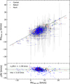 |
Fig. 2 Comparison between the RV measured in this work from the blue-arm and red-arm LAMOST MRS spectra (top panel). Different colors are used for the different subsamples of candidate members as indicated in the legend. The one-to-one relation is shown by the black dashed line. The RV differences (blue–red) displayed in the bottom panel show an average value of −1.4 km s−1 (black dashed line) and a standard deviation of 3.1 km s−1 (green dot-dashed lines). |
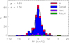 |
Fig. 3 RV distribution obtained with all the analyzed LAMOST-MRS spectra of the cluster members (red histogram) and for the three sub-samples, as indicated in the legend. The Gaussian fit is overplotted with a full black line; the center (μ) and dispersion (σ) of the Gaussian are also marked. |
3.2 Atmospheric parameters and projected rotation velocity
The comparison of blue- and red-arm values for the other stellar parameters (Teff, log g, [Fe/H], and v sin i) allows us to get reliable estimates of their errors and to highlight specific issues with them. As explained above, before obtaining the final parameters, we produced two sets of APs for each source from the analysis of the blue- and red-arm spectra, which can be compared as we did for the RVs.
For Teff, we observe a discrepancy between blue- and redarm values for Teff,red ≤ 4500 K (Fig. 4). As the coldest targets in this cluster are also the faintest, we suspect this can be the result of the low S/N in their blue-arm spectra. Another possibility is that the presence of spectral features strongly sensitive to the cold matter typical of starspots (T ≤ 4000 K) influences the determination of the temperature in the blue arm, leading to values lower than those of the pristine photosphere. In fact, it has been found that effective temperatures measured in young stars from near-infrared spectra (7000–10 000 Å) dominated by TiO bands, are systematically lower than those derived at optical wavelengths (e.g., Cottaar et al. 2014; Flores et al. 2022). As noted by Gangi et al. (2022), this offset is particularly noticeable in the temperature range between about 4000 and 4500 K, where it can even reach values of 500 K. This is the Teff range where the discrepancy is most evident in our data. A two-component model with synthetic spectra reproducing starspots and the photosphere is able to fit the spectral energy distribution of active pre-main sequence (PMS) stars (Gangi et al. 2022) and explain this discrepancy. Such a detailed modeling for a large source number is beyond the scope of our work. However, when calculating the weighted average of Teff based on S/N, χ2, or variance, the bluearm results usually weigh less for these cold objects, so the effect of starspots is mitigated. We note that neglecting stars colder than 4500 K the dispersion decreases from 277 K to 143 K, which is a value in agreement with the results of Frasca et al. (2022). These average Teff agree reasonably well with literature values (Sect. 3.3).
Regarding gravity, we find an overall good agreement between the blue-arm and red-arm results, with a handful of cases for which the blue-arm spectra gave rise to low gravity (log g < 4.0) when the red-arm log g is larger than 4.5 (see Fig. A.1). This corresponds again to cold stars with low S/N ratios in the blue arm that provided uncertain results, as also indicated by the large errors. The typical log g errors derived by ROTFIT but also by this comparison (after dividing the rms scatter by ![$\[\sqrt{2}\]$](/articles/aa/full_html/2025/06/aa53673-25/aa53673-25-eq10.png) ) are approximately 0.15 dex.
) are approximately 0.15 dex.
As for the metallicity, the agreement of blue- and red-arm values is very good (Fig. A.2). As expected for the members of a young cluster, all the targets display a near-solar metallicity with very few “extreme” values of [Fe/H] ≃ −0.4, mostly in the red arm. As for the other APs, the final metallicity reported in Table 1 is the weighted average of the values measured in the blue and red arm. The [Fe/H] distribution is shown in Fig. 5, where we distinguished the different subsamples as we did for the RV. The distribution peaks at small negative values of [Fe/H] and displays a slightly asymmetric shape with a tail towards negative [Fe/H]. The average metallicity of the cluster, [Fe/H] = −0.03 ± 0.06, is determined by fitting the [Fe/H] distribution with a Gaussian function, whose dispersion σ has been adopted as the error of the cluster metallicity. There is no clear distinction between the different subsamples, as also suggested by the values of μ and σ found for the more kinematically scattered population of the Hunt and Rebull subsamples, which are the same (within the errors) as those of the Cantat subsample.
As shown by Frasca et al. (2022) with Monte Carlo simulations, the resolution and sampling of the MRS LAMOST spectra do not allow for the measurement of v sin i values lower than 8 km s−1. Whenever we found a smaller value in at least one arm, this needed to be treated as a non-detection and flagged as an upper limit. A comparison of the blue-arm with the redarm v sin i shows a fairly good correlation and a low value floor for blue-arm spectra (v sin iblue), which extends up to v sin ired ≃ 30 km s−1 and translates into the tilted strip in Fig. 6. A similar behavior was found by Frasca et al. (2022). This happens when the red-arm spectra provided a poor constrain to v sin i due to the few absorption lines or to the presence of molecular bands. Some objects show the opposite behavior, that is, a range of v sin i values extending to about 30 km s−1 for which we found v sin i≃ 0 from the ROTFIT analysis of red-arm spectra. This is likely due to the low S/N of the blue-arm spectra or some flaws in them. Apart from these issues at low values of v sin i, we note that red values are systematically ≈5 km s−1 larger than the blues ones. We do not know the reason for this discrepancy, which could be related to the different shape of the spectra in the red and blue regions. However, the weighted average of the values obtained from the blue and red arm gives v sin i values that are in good agreement with those derived from APOGEE (see Sect. 3.3). These are the final values of v sin i that we adopt in this work and list in Table 1.
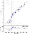 |
Fig. 4 Comparison of the Teff values derived from the blue- and redarm LAMOST-MRS spectra with ROTFIT. The meaning of lines and symbols is the same as in Fig. 2. We note the systematic discrepancy for Teff,red ≤ 4500 K. This boundary is given by the dash-dotted vertical line to guide the eye. |
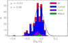 |
Fig. 5 [Fe/H] distribution for all the Pleiades members (red histogram) and for the three subsamples, as indicated in the legend. The Gaussian fit is overlaid with a black line; the center (μ) and dispersion (σ) of the Gaussian are also marked. |
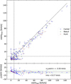 |
Fig. 6 Comparison of the v sin i values derived from the blue- and redarm LAMOST-MRS spectra with ROTFIT. The meaning of lines and symbols is the same as in Fig. 2. |
3.3 Data quality control: comparison with the literature
To check the accuracy of our values, we have compared the APs derived with ROTFIT on the LAMOST-MRS spectra with those available in the literature.
As regards the radial velocity, in Fig. 7 we show the comparison of our average RV values, corrected for the systematic offsets, with those measured by APOGEE with the ASPCAP pipeline and reported in the 17th data release of the Sloan Digital Sky Survey (SDSS APOGEE-2 DR17, Abdurro’uf et al. 2022) for the 205 sources in common between LAMOST and APOGEE. We note a small negative average offset of −2.0 km s−1 between our corrected RVs and APOGEE and an rms of the data dispersion around the mean of 3.8 km s−1. If we exclude the seven most discrepant points (|ΔRV| ≥ 3 · rms) the offset becomes −1.7 km s−1 and the rms decreases at 2.7 km s−1. It is worth noticing that these objects are on the tail of the RV distribution, which is peaked at about 5 km s−1 in both datasets (see Figs. 3 and 8). Moreover, three of these sources (#1, #2, and #4) have been already flagged as stars with variable RV (’RVvar’) in Table 1, according to the P(χ2) < 0.05 criterion. Details on these discrepant stars are provided in Appendix B.
The distribution of the average RVs of the 229 Pleiades members observed by APOGEE, which are contained in the SDSS APOGEE-2 DR17 (Abdurro’uf et al. 2022), is shown in Fig. 8. The center μ = 5.72 ± 0.02 km s−1 and dispersion σ = 0.88 ± 0.09 km s−1, where obtained, as for the ROTFIT RVs measured on LAMOST spectra, with a Gaussian fit. They again suggest a small negative offset (≈ −0.7 km/s) between ROTFIT–LAMOST and APOGEE and a smaller dispersion for the latter dataset, possibly due to their better accuracy.
The comparison of the ROTFIT Teff with those derived with LASP4 and the ASPCAP pipelines is shown in Fig. 9. One of the most striking feature of these scatter plots is the “boxy” shape, which is more evident in the comparison with LASP data. This pattern was already noted by Frasca et al. (2022), who interpreted it as a sort of “pile up” of the average parameters around those of the best (minimum χ2) template. This is not surprising, because ROTFIT does not apply any kind of interpolation or regularization between the parameters of the closest templates. Despite this pattern, the comparison with APOGEE indicates a scatter of about 247 K and an overall offset of ≈ −202 K, which is mostly due to the stars with TeffROT FIT < 4500 K. There is only one outstanding outlier in this plot, which is Gaia DR3 649494274606140 (= V357 Tau), with a Teff≃3950 K in the APOGEE catalog, for which we find instead 5955 K. The comparison with LASP displays a smaller offset of −68 K and an rms of ≈ 223 K that is due to the “boxy” shape of the scatter plot. Interestingly, V357 Tau does not appear as an outlier in this plot because its LASP temperature of 5907 K reported by Wang et al. (2021) is nearly identical to our value. We note that this star has a Gaia color GBP − GRP=1.85 mag, which is consistent with the APOGEE Teff, but its Re-normalized Unit Weight Error value, RUWE = 14.578 indicates a bad astrometric solution and could be related to the presence of an unresolved optical companion. Therefore, we have discarded this star from the following analysis. The comparison with APOGEE and LASP data suggests that our Teff determination is of sufficient quality for our purposes, as also witnessed by the rather smooth distribution of Gaia color index versus our Teff values (Fig. A.3).
The comparison of log g values of the present work with those derived with LASP and APOGEE is shown in Fig. A.4. The values agree well to each other with a small average offset (0.03–0.06 dex) and a small rms scatter of about 0.11 dex.
The comparison of v sin i values measured with ROTFIT in the present work with those derived with LASP, APOGEE, and the values reported in Hartman et al. (2010, which is a compilation of literature data mostly coming from Queloz et al. 1998 and Terndrup et al. 2000) and in Soderblom et al. (1993a) is shown in Fig. A.5. The ROTFIT values agree very well with the APOGEE ones derived with the ASPCAP pipeline, showing only a small residual scatter for the ROTFIT values less than or close to the LAMOST upper limit of 8 km s−1. The discrepant points at v sin iASPCAP = 96 km s−1 that are enclosed into red squares correspond to the maximum rotational broadening allowed for the ASPCAP pipeline (Jönsson et al. 2020). If we exclude these points, we find an offset of only ≈ 2 km s−1 with an rms dispersion of ≈7 km s−1. Another discrepant point is related to the F-type source Gaia-DR3 66832993955739776 (=HD 23567) (#1) for which we find v sin i = 90.1 km s−1 while ASPCAP reports 50 km s−1. This source is a δ Sct-type star for which a v sin i = 98.5 km s−1, in better agreement with our value, is reported by Solano & Fernley (1997). The comparison with the LASP results displays a bad correlation. In particular, the LASP values are systematically higher than ours by about 9 km s−1, on average. Moreover, the minimum v sin i in the LASP data is 27 km s−1, which is related to the method, the template grid (minimum Teff=5000 K), and the velocity steps adopted in the LASP pipeline (e.g., Zuo et al. 2024).
The agreement of our results with those reported by Hartman et al. (2010) and Soderblom et al. (1993a) is good, with average differences of about 1 km s−1 and dispersion of about 9 km s−1, as shown in the bottom panels of Fig. A.5. This strengthens the validity of our ROTFIT-based measures and suggests using the (few) v sin i values of LASP with caution.
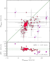 |
Fig. 7 Comparison between the RV measured in this work and APOGEE DR17 values (Abdurro’uf et al. 2022). The one-to-one relation is shown by the full line in the upper box. The RV differences between ROTFIT-LAMOST and APOGEE, ΔRV, are displayed in the lower box and show an average value of −2.01 km s−1 (dashed line) and a standard deviation of 3.79 km s−1 (dotted lines). The purple squares enclose the most discrepant points. |
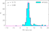 |
Fig. 8 RV distribution (cyan histogram) of the Pleiades members observed by APOGEE, as obtained with the average RV values reported in the 17th data release of SDSS (Abdurro’ uf et al. 2022). The Gaussian fit is overplotted with a full pink line; the center (μ) and dispersion (σ) of the Gaussian are also marked. |
 |
Fig. 9 Comparison between the Teff values measured in this work and those found in the literature. Left panel: ROTFIT versus APOGEE-2 DR17 Teff values (Jönsson et al. 2020). The color of symbols distinguishes the three subsamples as in the previous figures and indicated in the legend. The one-to-one relation is shown by the dashed line. The Teff differences between ROTFIT and APOGEE, ΔTeff, are displayed in the lower box. Right panel: ROTFIT versus LASP DR11 v1.0 Teff values (https://www.lamost.org/dr11/v1.0). The meaning of lines and symbols is as in the left panel. |
 |
Fig. 10 Comparison between the Prot values adopted in this work (from K2 or TESS) and those published by Hartman et al. (2010). The color of symbols distinguishes the three subsamples as indicated in the legend. The one-to-one relation is shown by the black dashed line. The green and purple dotted lines with slopes of 0.5 and 2, respectively, are also shown. The most discrepant stars are enclosed into squares in blue (for Prot reported in Rebull et al. 2016) and red (for Prot values derived in this work from TESS data). |
4 Rotation periods
As mentioned in Sect. 2.3, for most (178 out of 283) of the sources investigated by us the rotational periods, Prot, were derived by Rebull et al. (2016) from the analysis of Kepler-K2 photometry. For 89 of the remaining stars we were able to measure Prot from TESS data in three consecutive quarters, by means of a Lomb-Scargle periodogram analysis (Scargle 1982) to which the CLEAN deconvolution algorithm (Roberts et al. 1987) was applied. To validate the above period analysis we have selected a dozen stars analyzed by Rebull et al. (2016) with both short and long periods. We have retrieved and analyzed the TESS photometry in the three consecutive sectors 42,43, and 44. The results are shown in Fig. A.6 and are quoted in Table A.3. The Prot values are in excellent agreement, typically within 1% and always better than 5%, with each other. A sample of TESS light curves of both short- and long-period variables is shown in Fig. A.7. Typically, a single peak, corresponding to the rotational period, dominates the periodogram. In some cases, such as TIC 15902424 and TIC 427545153, the periodogram shows two close peaks and a beating pattern is apparent in the light curve. This behavior has been observed when two or more spotted areas are located at different latitudes and the star is rotating differentially (e.g., Frasca et al. 2011, and reference therein). We report the values of Prot in Table 1.
We have compared these Prot values with those of Hartman et al. (2010), which were derived from ground-based photometry collected at the Hungarian-made Automated Telescope Network (HATNet) or retrieved from the literature in a few cases. The results are shown in Fig. 10 along with the one-to-one relation (black dashed line). Most of the 187 targets in common with Hartman et al. (2010) display a very good agreement of Prot values and lie on the bisector of the plot. Among the 16 most discrepant objects marked in Fig. 10 and listed in Table B.1, 12 have Prot measured by Rebull et al. (2016), while for the last four Prot has been determined in the present work with the TESS photometry. In order to explain the differences observed, in Fig. 10 are also plotted the 2×Prot relations with slopes 0.5 (green dotted line) and 2 (purple dotted line), respectively. Objects near the green dotted line are those for which Hartman et al. (2010) derives a rotation period that is half of ours. This could be due to the temporal sampling and photometric precision of the ground-based data and to the presence of spots of similar size at nearly opposite longitudes during the HATNet observations mimicking a light curve with a single spot and half the period. This is clearly the case for #3, #4, #5, #11, and #12. In the opposite case, for data near the line with slope = 2, it could be that the duration of the K2 or TESS observations is insufficient to correctly determine the rotation period, but this is more likely to happen with rotators with periods of less than a fortnight.
Furthermore, to try to understand this discrepancy, we have retrieved and analyzed the TESS photometry in sectors 42, 43, and 44 of the first 12 stars, in the same way we did for the sources with no data in Rebull et al. (2016) and found the same period within the errors, suggesting that Rebull’s (and our) determination is very likely the correct value. We found only two exceptions, namely #8 for which we find Prot ≃ 13.5 d instead of 7.56 d measured by Rebull et al. (2016), and #9 for which we measure Prot ≃ 1.204 ± 0.005 d instead of 0.845 d. For the first object, adopting our Prot determination increases the discrepancy, considering the very small period of 0.333 d reported by Hartman et al. (2010). Moreover, we do not find any indication of high-frequency peaks in our periodogram; this, along with the low v sin i measured in our LAMOST spectra points to a long rotation period. For #9 our Prot determination is nearly identical to the Hartman et al. (2010) period (1.207 d), then resolving the discrepancy.
Regarding the remaining four stars, #13 to #16, as mentioned before, their periods are only measured by us from the TESS data. For #13 Hartman et al. (2010) found a period of 0.904 d while ours is 7.04 d, which is more consistent with the upper limit v sin i≤8 km s−1 or the value of 5 km s−1 measured by Queloz et al. (1998). Indeed, such a low v sin i would imply an inclination i < 10° with Prot=0.904 d, which is too small to produce a significant variation for ground-based observations. Moreover, no peak around 0.90 d is visible in our periodogram. For #14 Hartman et al. (2010) found a period of 7.50 d, almost twice our determination (4.24 d). However, a second peak with a slightly lower amplitude in our periodogram is found at Prot=7.60 d, which is close to the Hartman et al. (2010) determination. For #15 Hartman et al. (2010) found a period of 4.082 d, while our determination is 1.307 d without any indication of significant peaks at longer periods. This Prot value agrees with our determination of v sin i=39.2 km s−1, which excludes a longer rotation period. Interestingly, the Prot determination of 4.082 d quoted by Hartman et al. (2010) is an uncertain value reported by Marilli et al. (1997) that is likely a wrong determination.
The last discrepant source, #16 (= TIC 440686834 = Gaia DR3 64030785494725632), is a very puzzling object. Indeed, we find a large-amplitude variation with a period of about 15.3 days (see also Fig. A.7). In the high-frequency domain of the periodogram there is also a small amplitude (~30 times lower than the former) peak a Prot ≃ 0.215 d, which is indicated with a blue arrow in Fig. A.7 and corresponds to the rotation period reported by Hartman et al. (2010). This value of Prot is also consistent with the v sin i = 123.6 km s−1 measured by us. This object was classified by us as a possible SB2 on the basis of the appearance of the spectrum and the shape of the CCF peak that displays a broad and a narrow component (see Fig. A.8). It is not clear if it is a physical binary or an optical unresolved double. It is interesting to note that there is no bright source within 21″ in the Gaia DR3, but the Re-normalized Unit Weight Error value (RUWE) is 2.386. The RUWE is expected to be close to 1.0 when a single-star model fits the astrometric observations adequately. A value noticeably higher than 1.0, like in this case, may suggests that the source is either not a single star or presents challenges for the astrometric solution (Castro-Ginard et al. 2024). Therefore, we consider 0.215 d as the rotation period of the star with the broader lines. The Prot ≃ 15.3 d could be instead related to the narrow-lined component.
5 Chromospheric emission and lithium abundance
For stars belonging to young OCs both the chromospheric emission (traced by Balmer Hα in the LAMOST MRS spectra) and lithium absorption are age-dependent parameters (see, e.g., Jeffries 2014; Frasca et al. 2018, and references therein). As chromospheric emission in the Hα can only result in a small to moderate filling of the line core, depending on the activity level and on the photospheric flux of the star, the removal of the photospheric spectrum is mandatory. To this end, we have subtracted the non-active, lithium-poor template that best matches the final APs from each LAMOST red-arm spectrum. This template has been aligned to the target RV, rotationally broadened by the convolution with a rotational profile with the v sin i of the target and resampled on its spectral points. The “emission” Hα equivalent width, ![$\[W_{\mathrm{H} \alpha}^{\text {res}}\]$](/articles/aa/full_html/2025/06/aa53673-25/aa53673-25-eq11.png) , was measured by integrating the residual emission profile (see Fig. 11, top panel). We excluded the SB2s from this analysis and kept only the values of
, was measured by integrating the residual emission profile (see Fig. 11, top panel). We excluded the SB2s from this analysis and kept only the values of ![$\[W_{\mathrm{H} \alpha}^{\text {res}}\]$](/articles/aa/full_html/2025/06/aa53673-25/aa53673-25-eq12.png) significantly larger than zero, i.e. those larger or equal to their respective errors (256 sources). For the remaining single-lined sources, we adopted the error as the upper limit of the measure. These data are reported in Table 3, where we list the weighted average of the values measured in the individual spectra for stars with multiple observations.
significantly larger than zero, i.e. those larger or equal to their respective errors (256 sources). For the remaining single-lined sources, we adopted the error as the upper limit of the measure. These data are reported in Table 3, where we list the weighted average of the values measured in the individual spectra for stars with multiple observations.
The equivalent width of the Li I λ6708 Å absorption line (WLi) was also measured in the subtracted spectra where the blends with nearby photospheric lines have been removed (see Fig. 11, bottom panel). This allows us to get a better measure of WLi and a reliable estimate of its error, which was calculated as ![$\[\sigma_{W_{\mathrm{Li}}}=D \cdot \sqrt{\omega \Delta \lambda}\]$](/articles/aa/full_html/2025/06/aa53673-25/aa53673-25-eq13.png) , where D is the average dispersion of the flux values in the residual spectrum on the two sides of the line
, where D is the average dispersion of the flux values in the residual spectrum on the two sides of the line ![$\[D \simeq \frac{1}{S/N}\]$](/articles/aa/full_html/2025/06/aa53673-25/aa53673-25-eq14.png) , w is the integration width in wavelength units and Δλ (=0.15 Å) is the pixel size in wavelength units. This expression is similar to the formula proposed by Cayrel (1988). We were able to detect the lithium line (WLi larger than the error in at least one spectrum) for 224 objects, while for 52 of them we could only determine an upper limit. We did not measure WLi for the SB2 systems. For the stars with time-series spectra we calculated the weighted average of the individual values of WLi and took the weighted standard deviation or the standard error of the weighted mean (whenever greater than the former) as the error estimate. For the objects with only non-detections in all their spectra we took the lowest upper limit. These values are quoted in Table 4.
, w is the integration width in wavelength units and Δλ (=0.15 Å) is the pixel size in wavelength units. This expression is similar to the formula proposed by Cayrel (1988). We were able to detect the lithium line (WLi larger than the error in at least one spectrum) for 224 objects, while for 52 of them we could only determine an upper limit. We did not measure WLi for the SB2 systems. For the stars with time-series spectra we calculated the weighted average of the individual values of WLi and took the weighted standard deviation or the standard error of the weighted mean (whenever greater than the former) as the error estimate. For the objects with only non-detections in all their spectra we took the lowest upper limit. These values are quoted in Table 4.
The equivalent width of a chromospheric line is not the best diagnostic of magnetic activity, and more accurate indicators of chromospheric activity are the line flux in units of stellar surface, FHα, and the ratio between the line luminosity and bolometric luminosity, ![$\[R_{\mathrm{H} \alpha}^{\prime}\]$](/articles/aa/full_html/2025/06/aa53673-25/aa53673-25-eq15.png) , which have been evaluated according to Eqs. (2) and (3) of Frasca et al. (2022). These values are also reported in Table 3.
, which have been evaluated according to Eqs. (2) and (3) of Frasca et al. (2022). These values are also reported in Table 3.
The Hα flux and ![$\[R_{\mathrm{H} \alpha}^{\prime}\]$](/articles/aa/full_html/2025/06/aa53673-25/aa53673-25-eq17.png) are plotted as a function of Teff in Fig. 12. This plot also shows the dividing line between chromospherically active stars and objects still undergoing mass accretion, which was empirically determined by Frasca et al. (2015). As discussed by these authors, this boundary is close to the saturated chromospheric activity observed for main-sequence stars in young OCs (including the Pleiades), which has been found to be log
are plotted as a function of Teff in Fig. 12. This plot also shows the dividing line between chromospherically active stars and objects still undergoing mass accretion, which was empirically determined by Frasca et al. (2015). As discussed by these authors, this boundary is close to the saturated chromospheric activity observed for main-sequence stars in young OCs (including the Pleiades), which has been found to be log![$\[R_{\mathrm{H} \alpha}^{\prime}\]$](/articles/aa/full_html/2025/06/aa53673-25/aa53673-25-eq18.png) ≃ −3.3 by Barrado y Navascués & Martín (2003). Other authors, instead, estimate a lower value of log
≃ −3.3 by Barrado y Navascués & Martín (2003). Other authors, instead, estimate a lower value of log![$\[R_{\mathrm{H} \alpha}^{\prime}\]$](/articles/aa/full_html/2025/06/aa53673-25/aa53673-25-eq19.png) ≃ −3.7 for the saturation level (Fang et al. 2018). The
≃ −3.7 for the saturation level (Fang et al. 2018). The ![$\[R_{\mathrm{H} \alpha}^{\prime}\]$](/articles/aa/full_html/2025/06/aa53673-25/aa53673-25-eq20.png) values measured by us place all the Pleiades members in the region of chromospherically active sources as also seen in the Hα flux diagram. This is what is expected for a cluster of ≈100 Myr, for which the magnetospheric accretion from the circumstellar disks ended long ago. We note that the objects with the strongest activity, close to the saturation limit, are found among the coolest sources (Teff < 5000 K), as also found in previous works (e.g. Frasca et al. 2015; Fang et al. 2018). An average trend of decreasing chromospheric activity with the increase of Teff is also apparent in Fig. 12, where the most discrepant objects are those with upper limits in
values measured by us place all the Pleiades members in the region of chromospherically active sources as also seen in the Hα flux diagram. This is what is expected for a cluster of ≈100 Myr, for which the magnetospheric accretion from the circumstellar disks ended long ago. We note that the objects with the strongest activity, close to the saturation limit, are found among the coolest sources (Teff < 5000 K), as also found in previous works (e.g. Frasca et al. 2015; Fang et al. 2018). An average trend of decreasing chromospheric activity with the increase of Teff is also apparent in Fig. 12, where the most discrepant objects are those with upper limits in ![$\[W_{\mathrm{H} \alpha}^{\text {res}}\]$](/articles/aa/full_html/2025/06/aa53673-25/aa53673-25-eq21.png) . Most of them are warm stars (Teff > 6200 K) for which a small Hα excess emission is hard to detect against the strong photospheric flux. However, four objects with upper limits in
. Most of them are warm stars (Teff > 6200 K) for which a small Hα excess emission is hard to detect against the strong photospheric flux. However, four objects with upper limits in ![$\[R_{\mathrm{H} \alpha}^{\prime}\]$](/articles/aa/full_html/2025/06/aa53673-25/aa53673-25-eq22.png) are colder than 6000 K. They are, in decreasing Teff order, Gaia DR3 64770241424108032, Gaia DR3 64923279699744256, Gaia DR3 121349735399525632, and Gaia DR3 63916431989200256. With the exception of the penultimate one, these stars have a high membership probability (Pmemb = 1.0) according to Cantat-Gaudin et al. (2018) and a lithium abundance compatible with the cluster isochrone. However, they are all slow rotators (Prot>6 d), thus justifying their low chromospheric activity.
are colder than 6000 K. They are, in decreasing Teff order, Gaia DR3 64770241424108032, Gaia DR3 64923279699744256, Gaia DR3 121349735399525632, and Gaia DR3 63916431989200256. With the exception of the penultimate one, these stars have a high membership probability (Pmemb = 1.0) according to Cantat-Gaudin et al. (2018) and a lithium abundance compatible with the cluster isochrone. However, they are all slow rotators (Prot>6 d), thus justifying their low chromospheric activity.
For 257 sources with a measure of ![$\[W_{\mathrm{H} \alpha}^{\text {res}}\]$](/articles/aa/full_html/2025/06/aa53673-25/aa53673-25-eq31.png) or an upper limit we have the rotation periods (Sect. 4). This allowed us to investigate the dependence of chromospheric activity on parameters related to the efficiency of the dynamo action. We found a correlation between FHα and Prot with a Pearson’s coefficient ρ = −0.49. Another important parameter expressing the efficiency of the dynamo in convective stellar interiors is the Rossby number, RO, which is defined as the ratio of Prot and the convective turnover time, τcon. The latter is not a directly measurable quantity, but can be derived from theoretical models for MS stars or from calibrations as a function of temperature or color indices. We have used the empirical relation proposed by Wright et al. (2011, Eq. (10)) as a function of V − KS. The de-reddened color index (V − KS)0 is provided by Rebull et al. (2016) for the sources in their catalog. For the additional sources with periods determined by us, we have taken the V and KS magnitudes from the APASS (Henden et al. 2018) and 2MASS (Skrutskie et al. 2006) catalogs, respectively, and corrected the color index for the excess E(V − KS) = 0.11 mag as in Rebull et al. (2016). The correlation between activity indicators and RO is even better, with a coefficient ρ = −0.54 for FHα and −0.58 for
or an upper limit we have the rotation periods (Sect. 4). This allowed us to investigate the dependence of chromospheric activity on parameters related to the efficiency of the dynamo action. We found a correlation between FHα and Prot with a Pearson’s coefficient ρ = −0.49. Another important parameter expressing the efficiency of the dynamo in convective stellar interiors is the Rossby number, RO, which is defined as the ratio of Prot and the convective turnover time, τcon. The latter is not a directly measurable quantity, but can be derived from theoretical models for MS stars or from calibrations as a function of temperature or color indices. We have used the empirical relation proposed by Wright et al. (2011, Eq. (10)) as a function of V − KS. The de-reddened color index (V − KS)0 is provided by Rebull et al. (2016) for the sources in their catalog. For the additional sources with periods determined by us, we have taken the V and KS magnitudes from the APASS (Henden et al. 2018) and 2MASS (Skrutskie et al. 2006) catalogs, respectively, and corrected the color index for the excess E(V − KS) = 0.11 mag as in Rebull et al. (2016). The correlation between activity indicators and RO is even better, with a coefficient ρ = −0.54 for FHα and −0.58 for ![$\[R_{\mathrm{H} \alpha}^{\prime}\]$](/articles/aa/full_html/2025/06/aa53673-25/aa53673-25-eq32.png) . We have plotted the values of
. We have plotted the values of ![$\[R_{\mathrm{H} \alpha}^{\prime}\]$](/articles/aa/full_html/2025/06/aa53673-25/aa53673-25-eq33.png) as a function of the Rossby number in Fig. 13, distinguishing our targets by a Teff-dependent color code. The relation proposed by Newton et al. (2017) for nearby M dwarfs is overlapped with a dashed line. They fitted a canonical activity-rotation relation to their data, where the saturation level, for RO ≤ 0.21, was found to be log
as a function of the Rossby number in Fig. 13, distinguishing our targets by a Teff-dependent color code. The relation proposed by Newton et al. (2017) for nearby M dwarfs is overlapped with a dashed line. They fitted a canonical activity-rotation relation to their data, where the saturation level, for RO ≤ 0.21, was found to be log![$\[R_{\mathrm{H} \alpha}^{\prime}\]$](/articles/aa/full_html/2025/06/aa53673-25/aa53673-25-eq34.png) = −3.83. For larger values of RO they found a power-law decay with an exponent β = −1.7. A linear regression to our data for cold stars (Teff ≤ 4500 K) with RO > 0.21 also suggests a power-law decay with β = −1.94 ± 0.19 (green line in Fig. 13), which agrees, within the errors, with the results of Newton et al. (2017). However, for rapid rotators we find a higher saturation level, as already mentioned, with a slowly increasing trend towards the shortest values of RO. The fit of the data of cold stars (Teff ≤ 4500 K) with RO ≤ 0.21 gives rise to a slope of −1.18 ± 0.02 (cyan line in Fig. 13). A similar result was also found by Fang et al. (2018) by analyzing LAMOST-LRS data of young clusters including the Pleiades, where they found that a power law with slope −0.2 fitted the low RO domain better than a constant saturated value. This behavior has been also noticed by some researchers who used other activity diagnostics, such as the X-ray luminosity. For instance, Reiners et al. (2014) found a slow increase of the coronal activity in the saturated regime with a law
= −3.83. For larger values of RO they found a power-law decay with an exponent β = −1.7. A linear regression to our data for cold stars (Teff ≤ 4500 K) with RO > 0.21 also suggests a power-law decay with β = −1.94 ± 0.19 (green line in Fig. 13), which agrees, within the errors, with the results of Newton et al. (2017). However, for rapid rotators we find a higher saturation level, as already mentioned, with a slowly increasing trend towards the shortest values of RO. The fit of the data of cold stars (Teff ≤ 4500 K) with RO ≤ 0.21 gives rise to a slope of −1.18 ± 0.02 (cyan line in Fig. 13). A similar result was also found by Fang et al. (2018) by analyzing LAMOST-LRS data of young clusters including the Pleiades, where they found that a power law with slope −0.2 fitted the low RO domain better than a constant saturated value. This behavior has been also noticed by some researchers who used other activity diagnostics, such as the X-ray luminosity. For instance, Reiners et al. (2014) found a slow increase of the coronal activity in the saturated regime with a law ![$\[L_{\mathrm{X}} / L_{\text {bol }} \propto R_{\mathrm{O}}^{-0.16}\]$](/articles/aa/full_html/2025/06/aa53673-25/aa53673-25-eq35.png) . As already apparent in Fig. 12, it is once again shown that the hottest stars (Teff ≥ 6000 K) are those with the lowest activity level.
. As already apparent in Fig. 12, it is once again shown that the hottest stars (Teff ≥ 6000 K) are those with the lowest activity level.
Lithium is a fragile element that is burned in stellar interiors at temperature as low as 2.5 × 10⁶ K. It is progressively depleted from the stellar atmosphere in a way depending on the internal structure (i.e., stellar mass) when it reaches layers with the Li-burning temperature. Thus, its abundance can be used as an age proxy for stars cooler than about 6500 K. Theoretical or empirical (based on coeval star groups) isochrones are normally used to infer stellar ages (e.g., Jeffries 2014; Frasca et al. 2018). To this end, it is very important to determine as accurately as possible the age of the OCs used as a reference. In this sense, the Pleiades is one of the most widely used clusters and its age has been a long debated topic (discussed in more depth in Sect. 7). We derived the lithium abundance, A(Li), from our values of Teff, log g, and WLi by interpolating the curves of growth of Lind et al. (2009), which span the Teff range 4000–8000 K and log g from 1.0 to 5.0 and include non-LTE corrections. The errors of A(Li) have been calculated by propagating the Teff and WLi errors. These abundances are also listed in Table 4. A plot of A(Li) versus Teff is shown in Fig. 14 along with the upper envelopes of the A(Li) distributions for young OCs shown by Sestito & Randich (2005). Our data are correctly located between the upper envelopes corresponding to 300 and 100 Myr.
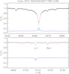 |
Fig. 11 Example of the subtraction of the best non-active, lithiumpoor template (red line) from the spectrum of the F9-type star Gaia-DR3 66462939577861248 = TIC 35205639 = HII 2786 (black dots) in the Hα (top panel) and Li I λ6708 Å (bottom panel) spectral regions. The difference spectrum (blue line), whose continuum has been arbitrarily shifted for clarity, reveals the chromospheric emission in the Hα core and emphasizes the lithium line, removing the blended photospheric lines. The green hatched areas represent the excess Hα emission and Li I absorption that were integrated to obtain |
![$\[W_{\mathrm{H} \alpha}^{\text {res}}\]$](/articles/aa/full_html/2025/06/aa53673-25/aa53673-25-eq16.png)
Chromospheric activity indicators: net Hα equivalent width (![$\[W_{\mathrm{H} \alpha}^{\text {res}}\]$](/articles/aa/full_html/2025/06/aa53673-25/aa53673-25-eq23.png) ), line flux (FHα), and luminosity ratio (
), line flux (FHα), and luminosity ratio (![$\[R_{\mathrm{H} \alpha}^{\prime}\]$](/articles/aa/full_html/2025/06/aa53673-25/aa53673-25-eq24.png) = LHα/Lbol).
= LHα/Lbol).
Lithium equivalent widths (WLi) and abundances (A(Li)).
 |
Fig. 12 Activity indicators. Left panel: Hα flux versus Teff. Right panel: |
![$\[R_{\mathrm{H} \alpha}^{\prime}\]$](/articles/aa/full_html/2025/06/aa53673-25/aa53673-25-eq27.png)
![$\[R_{\mathrm{H} \alpha}^{\prime}\]$](/articles/aa/full_html/2025/06/aa53673-25/aa53673-25-eq28.png)
![$\[R_{\mathrm{H} \alpha}^{\prime}\]$](/articles/aa/full_html/2025/06/aa53673-25/aa53673-25-eq29.png)
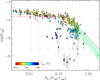 |
Fig. 13
|
![$\[R_{\mathrm{H} \alpha}^{\prime}\]$](/articles/aa/full_html/2025/06/aa53673-25/aa53673-25-eq30.png)
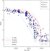 |
Fig. 14 Lithium abundance of the Pleiades members with LAMOST-MRS spectra as a function of Teff. Upper limits are highlighted with downward arrows. The upper envelopes of A(Li) for the IC 2602 (age ≈ 30 Myr), Pleiades, NGC 6475 (≈300 Myr), and Hyades (≈650 Myr) clusters adapted from Sestito & Randich (2005) are over-plotted. |
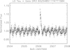 |
Fig. 15 Portion of a TESS light curve of LO Tau (= TIC 258067348) that displays a strong flare standing out above the rotational modulation. |
6 Flares
The multi-epoch LAMOST spectra offer the opportunity to study the variation of activity on different timescales. The data cadence is normally too scarce to properly sample variations of ![$\[W_{\mathrm{H} \alpha}^{\text {res}}\]$](/articles/aa/full_html/2025/06/aa53673-25/aa53673-25-eq36.png) produced by rotational modulation of chromospheric active regions, but it is helpful to characterize the variation range of the investigated sources and to detect flare events. The potential of these times series data will be exploited in forthcoming works. We only would like to mention three stars for which remarkable flares were detected.
produced by rotational modulation of chromospheric active regions, but it is helpful to characterize the variation range of the investigated sources and to detect flare events. The potential of these times series data will be exploited in forthcoming works. We only would like to mention three stars for which remarkable flares were detected.
The first case is Gaia-DR3 65254851174771584 (= TIC 258067348 = LO Tau). It is classified as an “eruptive variable” in Simbad, where a spectral type M2.9, based on APOGEE data (Birky et al. 2020), is reported. This is in very good agreement with our M2-type classification. The rapid rotation of this star is witnessed by the large value of v sin i = 68 km s−1, which agrees with the value of 80 km s−1 reported in the APOGEE DR17 catalog (Abdurro’uf et al. 2022) and with the rotational period Prot = 0.2587 d reported by Rebull et al. (2016). Several strong white-light flares are visible in the K2 and TESS light curves of this source (see Fig. 15 for an example).
In Fig. 16, we show the LAMOST MRS spectra of LO Tau taken from November 2019 to December 2021. The strong and broad Hα profile with emission wings extending up to ≈±500 km s−1 observed at MJD = 59216 is apparent. Another distinctive feature of this spectrum is the He I λ6678 Å emission line, which has never been observed during the quiescent phase. Emission in He I lines, notably the D3 λ5876Å line, has been reported during strong flares of RS CVn systems (e.g., Montes et al. 1997; García-Alvarez et al. 2003; Frasca et al. 2008; Cao et al. 2019) as well as in the strongest solar flares (e.g., Yakovkin et al. 2024). Unfortunately, our LAMOST spectra are not taken during K2 or TESS observations, and therefore no high-precision contemporaneous photometry is available.
Another strong flare has been clearly detected on Gaia-DR3 66555573432261376 (= TIC 640641946 = V371 Tau). V371 Tau has nearly the same spectral type as LO Tau (M2e, Prosser et al. 1991) but a lower v sin i = 5.9 km s−1 (Abdurro’uf et al. 2022). The lower rotation rate is confirmed by the longer Prot = 4.34 d we derived from the TESS light curves. From the analysis of the LAMOST MRS spectra, we found the same spectral type (M2V) but a different value of v sin i = 33.9 km s−1; we also noticed RV variations with a P(χ2) = 0.006 that make this star an SB1 candidate. Indeed, it is a visual binary composed of two stars with G = 14.5 mag and G = 15.3 mag separated by 2″, whose light entered the LAMOST fiber. The RV variation and the different v sin i values can be the result of the binarity. Although not explicitly mentioned in Simbad, this star displays frequent white-light flares in the space-based photometry. An example of a portion of a TESS light curve with two flares is shown in Fig. A.9. The spectrum acquired on MJD = 59216 displays a strong and broad Hα profile and He I emission, which are not observed in the quiescent phase (Fig. A.10).
The third object displaying a spectrum with flare characteristics is Gaia-DR3 66739982146803456 (= TIC 35155775 = V343 Tau = HII 1785). It is classified as a young stellar object in Simbad, where an M1.4 spectral type (Birky et al. 2020) and a v sin i = 7.2 km s−1 (Abdurro’uf et al. 2022) are reported. We find a slightly earlier spectral type (K6V) and a v sin i < 8 km s−1. The spectrum observed at MJD = 59531 (Fig. A.11) is typical of a flare event.
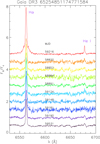 |
Fig. 16 LAMOST MRS photospheric-subtracted spectra of LO Tau in the spectral region containing the Hα and He I λ6678 Å line. The spectra have been sorted in time order from top to bottom (except for the uppermost one) and have been vertically shifted for clarity. The modified Julian day (MJD) is written next to the spectrum. The uppermost spectrum plotted with a red line displays a very strong and broad Hα profile as well as the He I line in emission, which is indicative of a flare event. |
7 Age of the Pleiades
The Pleiades, along with α Per and Hyades, is one of the best known OCs. It has been long used as benchmark to probe stellar evolution and calibrate the theoretical models due to its proximity and low foreground extinction.
However, the accepted (canonical) age for the Pleiades has changed by a factor of 2 in recent decades. To calculate the age of a cluster, the most widely used procedure is the isochrone-fitting method, in which theoretical models of different ages (isochrones) are superimposed on the CMD of the cluster until the isochrone that best reproduces the arrangement of the cluster members in the diagram is found. In this case, the position of giants (not present in the Pleiades) and stars in the upper MS, close to the turn-off point, are essential to make a good fit and, therefore, find a precise age. In the latter, the treatment of the convective mixing after exhausting the hydrogen in their cores plays a fundamental role in their (observable) properties. In the 1970s and 1980s, classical models (aside from using a different chemical composition) did not include the over-shooting as most modern models do. The resulting consequence is that the first age estimates for the Pleiades were ≤80 Myr (Hazlehurst & Thomas 1970; Simpson et al. 1970; Mermilliod 1981; Steele et al. 1993). On the contrary, nowadays, works devoted to it find older ages, about 110–160 Myr (Mazzei & Pigatto 1989; Gossage et al. 2018). However, even in current studies using an automated approach on a large cluster sample and taking Gaia distances into account (Kharchenko et al. 2013; Cantat-Gaudin et al. 2020; Dias et al. 2021; Hunt & Reffert 2024; Cavallo et al. 2024) the age spread still persists, giving values in the range ≈80–140 Myr.
The determination of the age of young clusters is affected not only by the lack of giant or turn-off stars, but also by the radius inflation caused the strong magnetic activity in their late-type members (e.g., Jackson et al. 2009; Jackson & Jeffries 2014b). The average radii of M-type dwarfs in the Pleiades have been found to be on average ~14% larger than inactive field M dwarfs (Jackson et al. 2018). Similar results have been found for other young MS or PMS clusters (Jackson et al. 2016). If not properly taken into account by the evolutionary models, the presence of starspots and magnetic fields, which make the low-mass stars redder and brighter, would lead to an underestimation of the age (e.g., Jeffries et al. 2023a).
On the other hand, an alternative to the isochrone-fitting method is the Li depletion boundary (LDB). This tool has proven to be very useful in determining the age of young OCs (≈20–200 Myr, see e.g. Basri et al. 1996; Stauffer et al. 1998; Barrado y Navascués et al. 2004). Indeed, this technique, according to Soderblom et al. (2014), would have the advantage of being model-independent, which is not a closed debate (Gossage et al. 2018). In any case, the results derived from the LDB for the Pleiades (using both MS stars and brown dwarfs) show a high level of agreement around 120 Myr (Basri et al. 1996; Stauffer et al. 1998; Martín et al. 2001; Dahm 2015). This age is currently the accepted canonical age for the Pleiades and is fully compatible with that obtained from isochronal analysis, whose stellar models include moderate rates of convective mixing and rotation.
Taking the results presented in Sect. 3.2 into account we estimated the cluster age from the fitting of empirical lithium isochrones. In this way, as done previously (see e.g. Alonso-Santiago et al. 2024a,b), we used the code EAGLES (Jeffries et al. 2023b). This code fits Li-depletion isochrones to the values of Teff (in the range 3000–6500 K) and WLi of a coeval stellar group. We note that EAGLES works better for clusters with a wide Teff distribution of members. This is indeed the case for our LAMOST WLi measurements. For our purposes, we have selected the best measurements, namely those with WLi errors less than 15 m Å (in total 144 objects), among the stars comprised in the working temperature range of the code. The results of the application of this code to our data are shown in Fig. 17. We find an age of about 118 ± 6 Myr, considering only the detections; if we include the upper limits, the age remains basically unchanged (122 ± 6 Myr). This age value is in line with the most recent determinations. We note that this result is very precise thanks to the large sample used, which covers a large part of the temperatures interval used for the isochrone fitting, as mentioned above. The opposite occurred in one of our previous works (Alonso-Santiago et al. 2024a), where we used a sample of three stars with similar temperatures only, resulting in a poor age estimate of 75 ± 36 Myr.
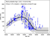 |
Fig. 17 Fit to the lithium depletion pattern of the Pleiades WLi measured in this work, obtained with the EAGLES code (Jeffries et al. 2023b). |
8 Spectroscopic binaries
The RV precision of LAMOST MRS is sufficient to detect binary systems and to derive their orbital elements and the physical parameters of the system components from the analysis of their RV curves (see, e.g., Pan et al. 2020; Wang et al. 2021). As mentioned in Sect. 3, in some spectra corresponding to ten sources we noted two peaks in the CCF that are significant in comparison with the CCF noise, which enabled us to classify these objects as SB2s. No stellar parameters are reported in Table 1 for these objects. In some cases the binary nature is questionable because the CCF only displays a distorted peak, which could be due to an unresolved companion or to starspots. We flagged these sources as “SB2?” in Table 1. Whenever an SB2 system is observed near the conjunctions, only one peak is visible in the CCF and the RV, measured with a single Gaussian fit; thus, it has to be considered as a “blended” value of the RVs of the two components, which is close to the velocity of the center of mass of the system.
In addition, we have objects with a single CCF peak that display a clear RV variation (SB1s). For these systems, for which a single component is visible in the spectrum, we report the APs. Some of these binaries were already known and their RVs and, in some cases, the orbital solutions were reported in the literature (e.g., Mermilliod et al. 1992; Torres et al. 2021). In the following, we show some examples of RV curves of well-studied systems, some of which, when treated as single stars, are among the most discrepant objects compared to the APOGEE RVs (Fig. 7). Our main aim is to show the agreement of our RV data with the RV curves in the literature. We also show cases of poorly studied or unknown system for which we could build an RV curve and come up with a preliminary orbital solution.
The first case is HII 571, discovered as an SB1 by Mermilliod et al. (1992), who also reported an orbital period of 15.9 days and provided an orbital solution. New data and a recent orbital solution were presented by Torres et al. (2021). The RV curve of HII 571 based on these data, three APOGEE epochs (Abdurro’uf et al. 2022), and one LAMOST-ROTFIT RV is presented in the left panel of Fig. 18, where the orbital solution of Torres et al. (2021) is also displayed. Two other SB1s discovered by Mermilliod et al. (1992) are HII 2172 (Porb ≃ 30.2 d) and HII 2406 (Porb ≃ 33.0 d), whose RV curves are also displayed in the middle and right panel of Fig. 18, respectively, along with the literature data and the solutions of Torres et al. (2021). We note that Torres et al. (2021) were able to detect the secondary CCF peak in their TRES spectra pf HII 2406, making this an SB2 system, but this component was not visible in the LAMOST spectra analyzed by us, so that we have only shown the RV curve of the much brighter primary star. The agreement of our LAMOST-MRS velocities derived with ROTFIT with the literature data is apparent.
Another interesting case is the short-period (Porb ≃ 5.69 d) double-lined binary DH794 discovered by Torres et al. (2021), who found a slightly eccentric orbit (e ≃ 0.013 ± 0.002). We could measure with ROTFIT the RVs of both components of this system in three LAMOST MRS spectra, while in the remaining three only the peak of the primary component could be identified. In addition, there are four APOGEE spectra taken with the 2.5-m telescope of the SDSS at the Apache Point Observatory. Since the radial velocities measured on these spectra and reported in the SDSS DR17 (Abdurro’uf et al. 2022) were derived by assuming the object as a single star, they are related to the primary (brighter) component only or are a “blended” measure taken when the two components are not well separated in wavelength. We therefore downloaded the APOGEE spectra5 and derived the velocities of both components by crosscorrelating the continuum-normalized APOGEE spectra with a template made with a BT-Settl synthetic spectrum (Allard et al. 2012), with [Fe/H]=0, log g=4.0 and Teff in the range 3800–4800 K, similar to what we did in Frasca et al. (2021) for a newly discovered SB2 system in Orion. Our LAMOST-ROTFIT RV measures and those we measured on the four DR17 APOGEE data are reported in Table A.4 and show a very good agreement with the Torres et al. (2021) data and orbital solution (Fig. 19).
The same holds true for HII 761, which was discovered as an SB1 system by Mermilliod et al. (1992) and subsequently classified as an SB2 by Torres et al. (2021) who were able to measure the RV of the secondary component, although with a lower accuracy than the primary, in their spectra. We were also able to detect the CCF peak of the secondary component in the APOGEE spectra and in most of the LAMOST-MRS ones and report these data in Table A.5. Our RV measures follow closely the circular orbital solution of Torres et al. (2021) (middle panel of Fig. 19). A third SB2 system, discovered by Torres et al. (2021), is HCG 495. The RV measured by us on three APOGEE and one LAMOST MRS spectra, reported in Table A.6 and displayed in the right panel of Fig. 19, allowed us to refine the orbital solution proposed by Torres et al. (2021) and the new orbital elements are listed in Table 5.
We discovered QQ Tau (= HII 1286) as a new SB2 system. It is classified as an “eruptive variable” (likely related to the strong flare activity detected by space photometry) in the Simbad database, with no indication of binarity. We have augmented the 13 RV values derived with ROTFIT from LAMOST MRS spectra taken from 14/11/2019 to 12/11/2021 with RV measurements based on six APOGEE spectra taken from 13/10/2011 to 21/09/2016. All these RVs are reported in Table 6. We applied the Lomb–Scargle periodogram (Scargle 1982) with the CLEAN deconvolution algorithm (Roberts et al. 1987) to the RV data of the primary and secondary component to search for the orbital period of the system, which turned out to be 2.462 days, in close agreement with the one we derived from the periodic analysis of the TESS photometry. Given the short period and the small number of RV points with relatively large errors we have searched for a circular orbit as a preliminary solution. We note that the solution improves if we apply a shift of +5 km s−1 to the LAMOST-MRS RVs. The RV curve and solution are shown in Fig. 20 and the orbital parameters are listed in Table 7. We remark that this is a preliminary solution and new medium- or high-resolution spectra are highly desirable to improve it.
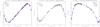 |
Fig. 18 Radial velocity curves of three single-lined binaries: HII 517 (left panel), HII 2172 (=HD 282965; middle panel), and HII 2406 (right panel). The RV data of Mermilliod et al. (1992) and Torres et al. (2021) are shown by purple and black dots, respectively, while the APOGEE DR17 data (Abdurro’uf et al. 2022) and our LAMOST RVs are plotted with red squares and asterisks, respectively. The orbital solutions are superimposed with a full blue line. |
Orbital parameters of HCG 495.
 |
Fig. 19 Radial velocity curves of three SB2 binaries: DH 794 (left panel), HII 761 (middle panel), and HCG 495 (right panel). The RV data of Torres et al. (2021) are shown by black dots and open circles for the primary and secondary component, respectively. The RVs of the primary and secondary components measured by us from the APOGEE DR17 spectra are plotted with purple filled and magenta open squares, respectively. Our LAMOST RVs are plotted with black and magenta asterisks for the primary and secondary component, respectively. The RV values measured near the conjunctions, when only one CCF peak is visible, are marked with green crosses. The orbital solution of Torres et al. (2021) is superimposed with a full blue and red line for the primary and secondary component, respectively. |
Heliocentric RVs of QQ Tau (= HII 1286).
 |
Fig. 20 Radial velocity curve of the newly discovered SB2 binary QQ Tau (= HII 1286). The RVs measured by us from the APOGEE spectra are marked with purple filled and red open squares, respectively. Our LAMOST MRS RVs are shown with black and magenta asterisks for the primary and secondary component, respectively. The RVs taken near the conjunctions, when only one peak is visible, are marked with large green X symbols. The RV solution for a circular orbit is represented by the full blue and red line for the primary and secondary component, respectively. |
9 Summary
We present the results of our analysis, performed with the code ROTFIT, of 1581 LAMOST medium-resolution spectra of cool (FGKM-type) stars that are candidate members of the Pleiades open cluster. We were able to determine the APs (Teff, log g, and [Fe/H]), the radial velocity (RV), and the projected rotational velocity (v sin i) for most of these spectra, corresponding to 283 different stars.
Due to systematic offsets in different runs of LAMOST, we corrected the RVs measured in the blue and red arms for all the target spectra using spectra of RV standard stars present in the same plates as our Pleiades samples. We discussed the RV distribution and spotted the stars with variable RV in our catalog. The average uncertainties for RV, Teff, log g, and [Fe/H] are about 2.1 km s−1, 277 K, 0.15 dex, and 0.09 dex, respectively. Typical v sin i uncertainties are 5–6 km s−1, but we could only measure values larger than 8 km s−1 due to the MRS resolution and sampling. We validated the accuracy of our APs by comparing them to values from APOGEE DR17 and other sources in the literature, demonstrating an overall good agreement and confirming the reliability of the methodology. The RV distribution of the cluster members peaks at about 5.0 km s−1 with a dispersion, measured by the σ of the fitted Gaussian, of 1.4 km s−1, in line with other determinations. The mean metallicity of the cluster was found to be [Fe/H] = −0.03 ± 0.06.
By subtracting the best-matching non-active, lithium-poor template spectra from each LAMOST red-arm spectrum, we measured the equivalent widths of the Balmer Hα core emission and Li I λ6708 Å absorption lines. This allowed us to investigate the chromospheric emission and lithium absorption for these Pleiades members. All our targets show a chromospheric activity level compatible with the young cluster age and most of the coolest (Teff<5000 K) members display a saturated activity level. For three sources with multi-epoch data, we acquired their spectra during flares, so they are characterized by strong and broad Hα profiles and the presence of the He I λ6678 Å emission line. From the lithium abundance of the late-type members (Teff<6500 K), we provide a robust determination of the cluster age, 118 ± 6 Myr, supporting the current accepted age for the Pleiades.
We also derived rotational periods (Prot) for 89 stars lacking Prot values in Rebull et al. (2016), using TESS data. We cross-matched our targets with those in Hartman et al. (2010) to compare Prot values. Among 187 targets in common, most showed excellent agreement, with 16 exhibiting significant discrepancies. For 12 of these having Rebull Prot values, we calculated their TESS Prot and finally confirmed that the measurements of Rebull (and our own) are most likely to be correct. Thanks to the values of Prot, we were able to investigate the dependence of activity on the period or the Rossby number (RO = Prot/τcon). Interestingly, we found that the stars in the saturated activity regime (RO ≲ 0.21) do not show a flat distribution of ![$\[R_{\mathrm{H} \alpha}^{\prime}\]$](/articles/aa/full_html/2025/06/aa53673-25/aa53673-25-eq37.png) but, rather, a slight enhancement with the decreasing Prot or Rossby number.
but, rather, a slight enhancement with the decreasing Prot or Rossby number.
Moreover, thanks to their RV variation in these time series data, we found 39 candidates to single-lined spectroscopic systems (SB1s) and ten double-lined binaries (SB2s) that have been identified on the basis of the double-peak shape of the cross-correlation function (CCF). Many of them had already been known as binaries from the literature, but some were not yet known. In particular, we discovered the object QQ Tau to be an SB2 system for which we also provide a preliminary orbital solution of the RV curve. We also present RV curves for some already known SB1s and SB2s, for which we were able to improve the solutions via the addition of our and APOGEE RVs.
This work not only strengthens our understanding of the relationship between rotation and magnetic activity in young stars, but it also highlights the importance of high-quality spectroscopic data for exploring key questions in stellar astrophysics. Our results, in addition to displaying a robust dataset for future research, provide a benchmark for theoretical models of stellar activity and evolution in young clusters, offering new insights into the complex interplay between rotation, magnetic activity, and lithium abundance.
Orbital parameters of QQ Tau (= HII 1216).
Data availability
Full Tables 1, 3, 4, and A.2 are available at the CDS via anonymous ftp to cdsarc.cds.unistra.fr (130.79.128.5) or via https://cdsarc.cds.unistra.fr/viz-bin/cat/J/A+A/698/A7
Acknowledgements
We are grateful to the anonymous referee for a careful reading of the manuscript and very useful suggestions that helped us to improve our work. Based on observations collected with the Large Sky Area Multi-Object Fiber Spectroscopic Telescope (LAMOST) located at the Xinglong observatory, China. Guoshoujing Telescope (the Large Sky Area Multi-Object Fibre Spectroscopic Telescope LAMOST) is a National Major Scientific Project built by the Chinese Academy of Sciences. Funding for the project has been provided by the National Development and Reform Commission. LAMOST is operated and managed by the National Astronomical Observatories, Chinese Academy of Sciences. Support from the Italian Ministero dell’Università e della Ricerca (MUR) is also acknowledged. AF acknowledges funding from the Large-Grant INAF YODA (YSOs Outflow, Disks and Accretion). JZ and JNF acknowledge the support of National Natural Science Foundation of China (NSFC) through the Grants 12090040, 12090042 and 12427804, and the science research grants from the China Manned Space Project. This research made use of SIMBAD and VIZIER databases, operated at the CDS, Strasbourg, France. This publication makes use of data products from the Two Micron All Sky Survey, which is a joint project of the University of Massachusetts and the Infrared Processing and Analysis Center/California Institute of Technology, funded by the National Aeronautics and Space Administration and the National Science Foundation. This publication makes use of data products from the Wide-field Infrared Survey Explorer, which is a joint project of the University of California, Los Angeles, and the Jet Propulsion Laboratory/California Institute of Technology, funded by the National Aeronautics and Space Administration.
Appendix A Additional tables and figures
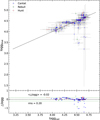 |
Fig. A.1 Comparison of the log g values derived from the blue- and red-arm LAMOST-MRS spectra with ROTFIT. The meaning of lines and symbols is the same as in Fig. 2. Note the few discrepant points at log gred > 4.5 dex. |
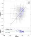 |
Fig. A.2 Comparison of the metallicity values derived from the blue- and red-arm LAMOST-MRS spectra with ROTFIT. The meaning of lines and symbols is the same as in Fig. 2. |
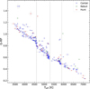 |
Fig. A.3 Comparison of the Gaia G--RP color and the Teff measured in this work for the stars belonging to the three subsamples as indicated in the legend. |
 |
Fig. A.4 Comparison between the log g measured in this work and those found in the literature. Left panel: ROTFIT versus APOGEE-2 DR17 values (Abdurro’uf et al. 2022). The color of symbols distinguishes the three subsamples as in the previous figures and indicated in the legend. The one-to-one relation is shown by the dashed line. The log g differences between ROTFIT and APOGEE, Δlog g, are displayed in the lower box. Right panel: Comparison with the LASP gravity values (https://www.lamost.org/dr11/v1.0). The meaning of lines and symbols is as in the left panel. |
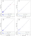 |
Fig. A.5 Comparison between the v sin i values measured in this work and those found in the literature. Top left panel: ROTFIT versus APOGEE-2 DR17 values (Abdurro’uf et al. 2022). The color of symbols distinguishes the three subsamples as in the previous figures and indicated in the legend. The one-to-one relation is shown by the dashed line. The v sin i differences between ROTFIT and APOGEE values, Δv sin i, are displayed in the lower box. Top right panel: Comparison with the LASP DR11 v1.0 v sin i values (https://www.lamost.org/dr11/v1.0). The meaning of lines and symbols is as in the left panel. Bottom left panel: ROTFIT versus (Hartman et al. 2010) v sin i values. Bottom right panel: ROTFIT versus Soderblom et al. (1993a) v sin i values. |
 |
Fig. A.6 Results of the period analysis of TESS light curves for a sample of Pleiades members observed also with Kepler-K2. In each panel, the inset in the upper left corner shows the cleaned periodogram computed by us in the TESS data, with the period marked by a vertical red line and indicated with red characters. The period derived by Rebull et al. (2016) with the K2 photometry is listed and marked in blue. The inset in the upper right corner of each panel displays the phased light curve. |
 |
Fig. A.7 TESS light curves for a sample of Pleiades members. In each panel, the inset in the upper left corner shows the cleaned periodogram, with the period marked by a vertical red line and indicated with red characters. The inset in the upper right corner displays the data phased with this period. |
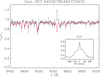 |
Fig. A.8 Red-arm spectrum of Gaia DR3 64030785494725632 (black line) with the best template (red line) found by ROTFIT that roughly fits the broad spectral lines. The cross-correlation function is displayed in the inset plot and clearly shows a broad and a narrow peak. |
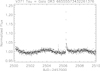 |
Fig. A.9 Portion of a TESS light curve of V371 Tau that displays two flares standing out above to the rotational modulation. |
RV corrections.
Radial velocities derived with ROTFIT from the red- and blue-arm MRS LAMOST spectra and the final corrected RV values.
Rotation periods derived with TESS and K2.
Heliocentric RVs of DH 794.
Heliocentric RVs of HII 761.
Heliocentric RVs of HCG 495.
Appendix B Discrepant objects
The seven discrepant objects in Fig. 7 are #1 (=Gaia-DR3 64148738180119680), #2 (=Gaia-DR3 64928605459180416 = HII 2406), #3 (=Gaia-DR3 65641913628380288 = V399 Tau), #4 (=Gaia-DR3 66771146429454592 = HII 2172 = HD 282965), #5 (=Gaia-DR3 66957994687842176 = V1091 Tau), #6 (=Gaia-DR3 69864313155605120 = HII 571), and #7 (=Gaia-DR3 65292234570088064=HD 23246). The objects #2, #4, and #6 are already known binaries (e.g., Torres et al. 2021). They are further investigated in Sect. 8 and their RV curves are shown in Fig. 18. For two of these sources (#3 and #6) there is only one LAMOST spectrum. The remaining three have a few LAMOST measures and do not show a clear RV variation in them. Further RV data are needed to check if they are SB1 systems. The stars with discrepant rotation periods with respect to Hartman et al. (2010), which are discussed in Sect. 4, are reported in Table B.1.
Objects with discrepant rotation period with respect to Hartman et al. (2010).
References
- Abdurro’uf, Accetta, K., Aerts, C., et al. 2022, ApJS, 259, 35 [NASA ADS] [CrossRef] [Google Scholar]
- Alfonso, J., & García-Varela, A. 2023, A&A, 677, A163 [NASA ADS] [CrossRef] [EDP Sciences] [Google Scholar]
- Allard, F., Homeier, D., & Freytag, B. 2012, Philos. Trans. Roy. Soc. Lond.. Ser. A, 370, 2765 [Google Scholar]
- Alonso-Santiago, J., Frasca, A., Bragaglia, A., et al. 2024a, A&A, 691, A317 [NASA ADS] [CrossRef] [EDP Sciences] [Google Scholar]
- Alonso-Santiago, J., Frasca, A., Catanzaro, G., et al. 2024b, A&A, 683, A75 [NASA ADS] [CrossRef] [EDP Sciences] [Google Scholar]
- Barnes, S. A. 2003, ApJ, 586, 464 [Google Scholar]
- Barrado y Navascués, D., & Martín, E. L. 2003, AJ, 126, 2997 [Google Scholar]
- Barrado y Navascués, D., Stauffer, J. R., & Jayawardhana, R. 2004, ApJ, 614, 386 [CrossRef] [Google Scholar]
- Barrado, D., Bouy, H., Bouvier, J., et al. 2016, A&A, 596, A113 [NASA ADS] [CrossRef] [EDP Sciences] [Google Scholar]
- Basri, G., Marcy, G. W., & Graham, J. R. 1996, ApJ, 458, 600 [NASA ADS] [CrossRef] [Google Scholar]
- Birky, J., Hogg, D. W., Mann, A. W., & Burgasser, A. 2020, ApJ, 892, 31 [Google Scholar]
- Bossini, D., Vallenari, A., Bragaglia, A., et al. 2019, A&A, 623, A108 [NASA ADS] [CrossRef] [EDP Sciences] [Google Scholar]
- Bouvier, J., Barrado, D., Moraux, E., et al. 2018, A&A, 613, A63 [NASA ADS] [CrossRef] [EDP Sciences] [Google Scholar]
- Cantat-Gaudin, T., Jordi, C., Vallenari, A., et al. 2018, A&A, 618, A93 [NASA ADS] [CrossRef] [EDP Sciences] [Google Scholar]
- Cantat-Gaudin, T., Anders, F., Castro-Ginard, A., et al. 2020, A&A, 640, A1 [NASA ADS] [CrossRef] [EDP Sciences] [Google Scholar]
- Cao, L., & Pinsonneault, M. H. 2022, MNRAS, 517, 2165 [NASA ADS] [CrossRef] [Google Scholar]
- Cao, D., Gu, S., Ge, J., et al. 2019, MNRAS, 482, 988 [NASA ADS] [CrossRef] [Google Scholar]
- Castro-Ginard, A., Penoyre, Z., Casey, A. R., et al. 2024, A&A, 688, A1 [NASA ADS] [CrossRef] [EDP Sciences] [Google Scholar]
- Cavallo, L., Spina, L., Carraro, G., et al. 2024, AJ, 167, 12 [NASA ADS] [CrossRef] [Google Scholar]
- Cayrel, R. 1988, in IAU Symposium, 132, The Impact of Very High S/N Spectroscopy on Stellar Physics, eds. G. Cayrel de Strobel, & M. Spite, 345 [Google Scholar]
- Cottaar, M., Covey, K. R., Meyer, M. R., et al. 2014, ApJ, 794, 125 [NASA ADS] [CrossRef] [Google Scholar]
- Cui, X.-Q., Zhao, Y.-H., Chu, Y.-Q., et al. 2012, RA&A, 12, 1197 [Google Scholar]
- Dahm, S. E. 2015, ApJ, 813, 108 [Google Scholar]
- Dias, W. S., Monteiro, H., Moitinho, A., et al. 2021, MNRAS, 504, 356 [NASA ADS] [CrossRef] [Google Scholar]
- Dinnbier, F., & Kroupa, P. 2020, A&A, 640, A85 [EDP Sciences] [Google Scholar]
- Fang, X.-S., Zhao, G., Zhao, J.-K., Chen, Y.-Q., & Bharat Kumar, Y. 2016, MNRAS, 463, 2494 [NASA ADS] [CrossRef] [Google Scholar]
- Fang, X.-S., Zhao, G., Zhao, J.-K., & Bharat Kumar, Y. 2018, MNRAS, 476, 908 [NASA ADS] [CrossRef] [Google Scholar]
- Feiden, G. A., & Chaboyer, B. 2013, ApJ, 779, 183 [Google Scholar]
- Feiden, G. A., & Chaboyer, B. 2014, ApJ, 789, 53 [NASA ADS] [CrossRef] [Google Scholar]
- Flores, C., Connelley, M. S., Reipurth, B., & Duchêne, G. 2022, ApJ, 925, 21 [NASA ADS] [CrossRef] [Google Scholar]
- Frasca, A., Guillout, P., Marilli, E., et al. 2006, A&A, 454, 301 [NASA ADS] [CrossRef] [EDP Sciences] [Google Scholar]
- Frasca, A., Biazzo, K., Taş, G., Evren, S., & Lanzafame, A. C. 2008, A&A, 479, 557 [NASA ADS] [CrossRef] [EDP Sciences] [Google Scholar]
- Frasca, A., Fröhlich, H. E., Bonanno, A., et al. 2011, A&A, 532, A81 [NASA ADS] [CrossRef] [EDP Sciences] [Google Scholar]
- Frasca, A., Biazzo, K., Lanzafame, A. C., et al. 2015, A&A, 575, A4 [NASA ADS] [CrossRef] [EDP Sciences] [Google Scholar]
- Frasca, A., Guillout, P., Klutsch, A., et al. 2018, A&A, 612, A96 [NASA ADS] [CrossRef] [EDP Sciences] [Google Scholar]
- Frasca, A., Boffin, H. M. J., Manara, C. F., et al. 2021, A&A, 656, A138 [NASA ADS] [CrossRef] [EDP Sciences] [Google Scholar]
- Frasca, A., Molenda-Żakowicz, J., Alonso-Santiago, J., et al. 2022, A&A, 664, A78 [NASA ADS] [CrossRef] [EDP Sciences] [Google Scholar]
- Gaia Collaboration (Babusiaux, C., et al.) 2018, A&A, 616, A10 [NASA ADS] [CrossRef] [EDP Sciences] [Google Scholar]
- Gaia Collaboration (Vallenari, A., et al.) 2023, A&A, 674, A1 [NASA ADS] [CrossRef] [EDP Sciences] [Google Scholar]
- Gangi, M., Antoniucci, S., Biazzo, K., et al. 2022, A&A, 667, A124 [NASA ADS] [CrossRef] [EDP Sciences] [Google Scholar]
- García-Alvarez, D., Foing, B. H., Montes, D., et al. 2003, A&A, 397, 285 [NASA ADS] [CrossRef] [EDP Sciences] [Google Scholar]
- Gossage, S., Conroy, C., Dotter, A., et al. 2018, ApJ, 863, 67 [Google Scholar]
- Guo, Z., Gully-Santiago, M., & Herczeg, G. J. 2018, ApJ, 868, 143 [Google Scholar]
- Hartman, J. D., Bakos, G. Á., Kovács, G., & Noyes, R. W. 2010, MNRAS, 408, 475 [Google Scholar]
- Hazlehurst, J., & Thomas, H. C. 1970, MNRAS, 150, 311 [Google Scholar]
- Henden, A. A., Levine, S., Terrell, D., et al. 2018, in American Astronomical Society Meeting Abstracts, 232, 223.06 [NASA ADS] [Google Scholar]
- Heyl, J., Caiazzo, I., & Richer, H. B. 2022, ApJ, 926, 132 [NASA ADS] [CrossRef] [Google Scholar]
- Huang, Y., Liu, X. W., Chen, B. Q., et al. 2018, AJ, 156, 90 [Google Scholar]
- Huang, C. X., Vanderburg, A., Pál, A., et al. 2020, RNAS, 4, 204 [Google Scholar]
- Hunt, E. L., & Reffert, S. 2024, A&A, 686, A42 [NASA ADS] [CrossRef] [EDP Sciences] [Google Scholar]
- Jackson, R. J., & Jeffries, R. D. 2014a, MNRAS, 445, 4306 [Google Scholar]
- Jackson, R. J., & Jeffries, R. D. 2014b, MNRAS, 441, 2111 [Google Scholar]
- Jackson, R. J., Jeffries, R. D., & Maxted, P. F. L. 2009, MNRAS, 399, L89 [NASA ADS] [CrossRef] [Google Scholar]
- Jackson, R. J., Jeffries, R. D., Randich, S., et al. 2016, A&A, 586, A52 [NASA ADS] [CrossRef] [EDP Sciences] [Google Scholar]
- Jackson, R. J., Deliyannis, C. P., & Jeffries, R. D. 2018, MNRAS, 476, 3245 [NASA ADS] [CrossRef] [Google Scholar]
- Jeffries, R. D. 2014, in EAS Publications Series, 65, eds. Y. Lebreton, D. Valls-Gabaud, & C. Charbonnel, 289 [Google Scholar]
- Jeffries, R. D., Jackson, R. J., & Binks, A. S. 2023a, MNRAS, 526, 1260 [Google Scholar]
- Jeffries, R. D., Jackson, R. J., Wright, N. J., et al. 2023b, MNRAS, 523, 802 [Google Scholar]
- Jönsson, H., Holtzman, J. A., Allende Prieto, C., et al. 2020, AJ, 160, 120 [Google Scholar]
- Kharchenko, N. V., Piskunov, A. E., Schilbach, E., Röser, S., & Scholz, R. D. 2013, A&A, 558, A53 [NASA ADS] [CrossRef] [EDP Sciences] [Google Scholar]
- Krumholz, M. R., McKee, C. F., & Bland-Hawthorn, J. 2019, ARA&A, 57, 227 [NASA ADS] [CrossRef] [Google Scholar]
- Lind, K., Asplund, M., & Barklem, P. S. 2009, A&A, 503, 541 [NASA ADS] [CrossRef] [EDP Sciences] [Google Scholar]
- Liu, N., Fu, J.-N., Zong, W., et al. 2019, RA&A, 19, 075 [Google Scholar]
- Liu, C., Fu, J., Shi, J., et al. 2020, arXiv e-prints [arXiv:2005.07210] [Google Scholar]
- López-Morales, M. 2007, ApJ, 660, 732 [Google Scholar]
- Luo, A. L., Zhao, Y.-H., Zhao, G., et al. 2015, RA&A, 15, 1095 [Google Scholar]
- Marilli, E., Catalano, S., & Frasca, A. 1997, Mem. Soc. Astron. Italiana, 68, 895 [Google Scholar]
- Martín, E. L., Dahm, S., & Pavlenko, Y. 2001, in Astronomical Society of the Pacific Conference Series, 245, Astrophysical Ages and Times Scales, eds. T. von Hippel, C. Simpson, & N. Manset, 349 [Google Scholar]
- Mazzei, P., & Pigatto, L. 1989, A&A, 213, L1 [NASA ADS] [Google Scholar]
- Mermilliod, J. C. 1981, A&A, 97, 235 [NASA ADS] [Google Scholar]
- Mermilliod, J. C., Rosvick, J. M., Duquennoy, A., & Mayor, M. 1992, A&A, 265, 513 [NASA ADS] [Google Scholar]
- Montes, D., Fernandez-Figueroa, M. J., de Castro, E., & Sanz-Forcada, J. 1997, A&AS, 125, 263 [NASA ADS] [CrossRef] [EDP Sciences] [Google Scholar]
- Morales, J. C., Ribas, I., & Jordi, C. 2008, A&A, 478, 507 [NASA ADS] [CrossRef] [EDP Sciences] [Google Scholar]
- Moultaka, J., Ilovaisky, S. A., Prugniel, P., & Soubiran, C. 2004, PASP, 116, 693 [NASA ADS] [CrossRef] [Google Scholar]
- Newton, E. R., Irwin, J., Charbonneau, D., et al. 2017, ApJ, 834, 85 [Google Scholar]
- Pan, Y., Fu, J.-N., Zong, W., et al. 2020, ApJ, 905, 67 [NASA ADS] [CrossRef] [Google Scholar]
- Press, W. H., Teukolsky, S. A., Vetterling, W. T., & Flannery, B. P. 1992, Numerical recipes in FORTRAN. The art of scientific computing (Cambridge: University Press) [Google Scholar]
- Prosser, C. F., Stauffer, J., & Kraft, R. P. 1991, AJ, 101, 1361 [NASA ADS] [CrossRef] [Google Scholar]
- Queloz, D., Allain, S., Mermilliod, J. C., Bouvier, J., & Mayor, M. 1998, A&A, 335, 183 [Google Scholar]
- Rebull, L. M., Stauffer, J. R., Bouvier, J., et al. 2016, AJ, 152, 113 [Google Scholar]
- Reiners, A., Schüssler, M., & Passegger, V. M. 2014, ApJ, 794, 144 [Google Scholar]
- Ricker, G. R., Winn, J. N., Vanderspek, R., et al. 2015, J. Astron. Telesc. Instrum. Syst., 1, 014003 [Google Scholar]
- Roberts, D. H., Lehar, J., & Dreher, J. W. 1987, AJ, 93, 968 [Google Scholar]
- Scargle, J. D. 1982, ApJ, 263, 835 [Google Scholar]
- Sestito, P., & Randich, S. 2005, A&A, 442, 615 [NASA ADS] [CrossRef] [EDP Sciences] [Google Scholar]
- Simpson, E., Hills, R. E., Hoffman, W., et al. 1970, ApJ, 159, 895 [NASA ADS] [CrossRef] [Google Scholar]
- Skrutskie, M. F., Cutri, R. M., Stiening, R., et al. 2006, AJ, 131, 1163 [NASA ADS] [CrossRef] [Google Scholar]
- Soderblom, D. R., Hillenbrand, L. A., Jeffries, R. D., Mamajek, E. E., & Naylor, T. 2014, in Protostars and Planets VI, eds. H. Beuther, R. S. Klessen, C. P. Dullemond, & T. Henning, 219 [Google Scholar]
- Soderblom, D. R., Jones, B. F., Balachandran, S., et al. 1993a, AJ, 106, 1059 [Google Scholar]
- Soderblom, D. R., Stauffer, J. R., Hudon, J. D., & Jones, B. F. 1993b, ApJS, 85, 315 [Google Scholar]
- Solano, E., & Fernley, J. 1997, A&AS, 122, 131 [NASA ADS] [CrossRef] [EDP Sciences] [Google Scholar]
- Somers, G., & Pinsonneault, M. H. 2014, ApJ, 790, 72 [NASA ADS] [CrossRef] [Google Scholar]
- Somers, G., & Pinsonneault, M. H. 2015a, ApJ, 807, 174 [Google Scholar]
- Somers, G., & Pinsonneault, M. H. 2015b, MNRAS, 449, 4131 [Google Scholar]
- Somers, G., & Stassun, K. G. 2017, AJ, 153, 101 [NASA ADS] [CrossRef] [Google Scholar]
- Soubiran, C., Jasniewicz, G., Chemin, L., et al. 2018, A&A, 616, A7 [NASA ADS] [CrossRef] [EDP Sciences] [Google Scholar]
- Stassun, K. G., Kratter, K. M., Scholz, A., & Dupuy, T. J. 2012, ApJ, 756, 47 [NASA ADS] [Google Scholar]
- Stauffer, J. R., Schultz, G., & Kirkpatrick, J. D. 1998, ApJ, 499, L199 [NASA ADS] [CrossRef] [Google Scholar]
- Steele, I. A., Jameson, R. F., & Hambly, N. C. 1993, MNRAS, 263, 647 [NASA ADS] [CrossRef] [Google Scholar]
- Terndrup, D. M., Stauffer, J. R., Pinsonneault, M. H., et al. 2000, AJ, 119, 1303 [NASA ADS] [CrossRef] [Google Scholar]
- Torres, C. A. O., Quast, G. R., da Silva, L., et al. 2006, A&A, 460, 695 [NASA ADS] [CrossRef] [EDP Sciences] [Google Scholar]
- Torres, G., Latham, D. W., & Quinn, S. N. 2021, ApJ, 921, 117 [Google Scholar]
- Wanderley, F., Cunha, K., Kochukhov, O., et al. 2024, ApJ, 971, 112 [NASA ADS] [CrossRef] [Google Scholar]
- Wang, S.-G., Su, D.-Q., Chu, Y.-Q., Cui, X., & Wang, Y.-N. 1996, Appl. Opt., 35, 5155 [NASA ADS] [CrossRef] [Google Scholar]
- Wang, R., Luo, A. L., Chen, J. J., et al. 2019, ApJS, 244, 27 [NASA ADS] [CrossRef] [Google Scholar]
- Wang, J., Fu, J., Niu, H., et al. 2021, MNRAS, 504, 4302 [NASA ADS] [CrossRef] [Google Scholar]
- Wright, N. J., Drake, J. J., Mamajek, E. E., & Henry, G. W. 2011, ApJ, 743, 48 [Google Scholar]
- Xing, X., Zhai, C., Du, H., et al. 1998, SPIE Conf. Ser., 3352, 839 [NASA ADS] [Google Scholar]
- Yakovkin, I. I., Lozitska, N. I., & Lozitsky, V. G. 2024, Universe, 10, 262 [Google Scholar]
- Zhang, B., Li, J., Yang, F., et al. 2021, ApJS, 256, 14 [NASA ADS] [CrossRef] [Google Scholar]
- Zong, W., Fu, J.-N., De Cat, P., et al. 2018, ApJS, 238, 30 [NASA ADS] [CrossRef] [Google Scholar]
- Zong, W., Fu, J.-N., De Cat, P., et al. 2020, ApJS, 251, 15 [NASA ADS] [CrossRef] [Google Scholar]
- Zuo, F., Luo, A. L., Du, B., et al. 2024, ApJS, 271, 4 [NASA ADS] [CrossRef] [Google Scholar]
![$\[W=c \sqrt{1 / R_{\text {MRS }}^{2}-1 / R_{\text {ELODIE }}^{2}} \text{km s}^{-1}\]$](/articles/aa/full_html/2025/06/aa53673-25/aa53673-25-eq38.png)
Available at http://skyserver.sdss.org/dr17/
All Tables
Radial velocity standard stars in the fields of LAMOST observations used in this paper.
Chromospheric activity indicators: net Hα equivalent width (), line flux (FHα), and luminosity ratio ( = LHα/Lbol).
Radial velocities derived with ROTFIT from the red- and blue-arm MRS LAMOST spectra and the final corrected RV values.
All Figures
|
Fig. 1 Left panel: spatial distribution of the Pleiades members according to Hunt & Reffert (2024, purple dots) and Cantat-Gaudin et al. (2018, blue dots). The symbol size scales with the G magnitude. The green diamonds mark the K2 variable stars in Rebull et al. (2016) that are not members according to either Hunt & Reffert (2024) or Cantat-Gaudin et al. (2018). Red dots represent the stars observed with LAMOST MRS. The meaning of the symbols is also indicated in the legend. Middle panel: color–magnitude diagram of the same sources. Right panel: proper motion diagram of all the Gaia DR3 sources with G ≤ 15 mag (small grey dots) in the field of the Pleiades (center coordinates RA(2000) = 03h46m, Dec(2000) = +24°06′, radius 4°). The Pleiades members are highlighted with the same symbols as in the other panels. The cyan asterisk denotes the average proper motion of the cluster according to Hunt & Reffert (2024) and the cyan ellipse is the 3σ contour. |
| In the text | |
|
Fig. 2 Comparison between the RV measured in this work from the blue-arm and red-arm LAMOST MRS spectra (top panel). Different colors are used for the different subsamples of candidate members as indicated in the legend. The one-to-one relation is shown by the black dashed line. The RV differences (blue–red) displayed in the bottom panel show an average value of −1.4 km s−1 (black dashed line) and a standard deviation of 3.1 km s−1 (green dot-dashed lines). |
| In the text | |
|
Fig. 3 RV distribution obtained with all the analyzed LAMOST-MRS spectra of the cluster members (red histogram) and for the three sub-samples, as indicated in the legend. The Gaussian fit is overplotted with a full black line; the center (μ) and dispersion (σ) of the Gaussian are also marked. |
| In the text | |
|
Fig. 4 Comparison of the Teff values derived from the blue- and redarm LAMOST-MRS spectra with ROTFIT. The meaning of lines and symbols is the same as in Fig. 2. We note the systematic discrepancy for Teff,red ≤ 4500 K. This boundary is given by the dash-dotted vertical line to guide the eye. |
| In the text | |
|
Fig. 5 [Fe/H] distribution for all the Pleiades members (red histogram) and for the three subsamples, as indicated in the legend. The Gaussian fit is overlaid with a black line; the center (μ) and dispersion (σ) of the Gaussian are also marked. |
| In the text | |
|
Fig. 6 Comparison of the v sin i values derived from the blue- and redarm LAMOST-MRS spectra with ROTFIT. The meaning of lines and symbols is the same as in Fig. 2. |
| In the text | |
|
Fig. 7 Comparison between the RV measured in this work and APOGEE DR17 values (Abdurro’uf et al. 2022). The one-to-one relation is shown by the full line in the upper box. The RV differences between ROTFIT-LAMOST and APOGEE, ΔRV, are displayed in the lower box and show an average value of −2.01 km s−1 (dashed line) and a standard deviation of 3.79 km s−1 (dotted lines). The purple squares enclose the most discrepant points. |
| In the text | |
|
Fig. 8 RV distribution (cyan histogram) of the Pleiades members observed by APOGEE, as obtained with the average RV values reported in the 17th data release of SDSS (Abdurro’ uf et al. 2022). The Gaussian fit is overplotted with a full pink line; the center (μ) and dispersion (σ) of the Gaussian are also marked. |
| In the text | |
|
Fig. 9 Comparison between the Teff values measured in this work and those found in the literature. Left panel: ROTFIT versus APOGEE-2 DR17 Teff values (Jönsson et al. 2020). The color of symbols distinguishes the three subsamples as in the previous figures and indicated in the legend. The one-to-one relation is shown by the dashed line. The Teff differences between ROTFIT and APOGEE, ΔTeff, are displayed in the lower box. Right panel: ROTFIT versus LASP DR11 v1.0 Teff values (https://www.lamost.org/dr11/v1.0). The meaning of lines and symbols is as in the left panel. |
| In the text | |
|
Fig. 10 Comparison between the Prot values adopted in this work (from K2 or TESS) and those published by Hartman et al. (2010). The color of symbols distinguishes the three subsamples as indicated in the legend. The one-to-one relation is shown by the black dashed line. The green and purple dotted lines with slopes of 0.5 and 2, respectively, are also shown. The most discrepant stars are enclosed into squares in blue (for Prot reported in Rebull et al. 2016) and red (for Prot values derived in this work from TESS data). |
| In the text | |
|
Fig. 11 Example of the subtraction of the best non-active, lithiumpoor template (red line) from the spectrum of the F9-type star Gaia-DR3 66462939577861248 = TIC 35205639 = HII 2786 (black dots) in the Hα (top panel) and Li I λ6708 Å (bottom panel) spectral regions. The difference spectrum (blue line), whose continuum has been arbitrarily shifted for clarity, reveals the chromospheric emission in the Hα core and emphasizes the lithium line, removing the blended photospheric lines. The green hatched areas represent the excess Hα emission and Li I absorption that were integrated to obtain |
| In the text | |
|
Fig. 12 Activity indicators. Left panel: Hα flux versus Teff. Right panel: |
| In the text | |
|
Fig. 13
|
| In the text | |
|
Fig. 14 Lithium abundance of the Pleiades members with LAMOST-MRS spectra as a function of Teff. Upper limits are highlighted with downward arrows. The upper envelopes of A(Li) for the IC 2602 (age ≈ 30 Myr), Pleiades, NGC 6475 (≈300 Myr), and Hyades (≈650 Myr) clusters adapted from Sestito & Randich (2005) are over-plotted. |
| In the text | |
|
Fig. 15 Portion of a TESS light curve of LO Tau (= TIC 258067348) that displays a strong flare standing out above the rotational modulation. |
| In the text | |
|
Fig. 16 LAMOST MRS photospheric-subtracted spectra of LO Tau in the spectral region containing the Hα and He I λ6678 Å line. The spectra have been sorted in time order from top to bottom (except for the uppermost one) and have been vertically shifted for clarity. The modified Julian day (MJD) is written next to the spectrum. The uppermost spectrum plotted with a red line displays a very strong and broad Hα profile as well as the He I line in emission, which is indicative of a flare event. |
| In the text | |
|
Fig. 17 Fit to the lithium depletion pattern of the Pleiades WLi measured in this work, obtained with the EAGLES code (Jeffries et al. 2023b). |
| In the text | |
|
Fig. 18 Radial velocity curves of three single-lined binaries: HII 517 (left panel), HII 2172 (=HD 282965; middle panel), and HII 2406 (right panel). The RV data of Mermilliod et al. (1992) and Torres et al. (2021) are shown by purple and black dots, respectively, while the APOGEE DR17 data (Abdurro’uf et al. 2022) and our LAMOST RVs are plotted with red squares and asterisks, respectively. The orbital solutions are superimposed with a full blue line. |
| In the text | |
|
Fig. 19 Radial velocity curves of three SB2 binaries: DH 794 (left panel), HII 761 (middle panel), and HCG 495 (right panel). The RV data of Torres et al. (2021) are shown by black dots and open circles for the primary and secondary component, respectively. The RVs of the primary and secondary components measured by us from the APOGEE DR17 spectra are plotted with purple filled and magenta open squares, respectively. Our LAMOST RVs are plotted with black and magenta asterisks for the primary and secondary component, respectively. The RV values measured near the conjunctions, when only one CCF peak is visible, are marked with green crosses. The orbital solution of Torres et al. (2021) is superimposed with a full blue and red line for the primary and secondary component, respectively. |
| In the text | |
|
Fig. 20 Radial velocity curve of the newly discovered SB2 binary QQ Tau (= HII 1286). The RVs measured by us from the APOGEE spectra are marked with purple filled and red open squares, respectively. Our LAMOST MRS RVs are shown with black and magenta asterisks for the primary and secondary component, respectively. The RVs taken near the conjunctions, when only one peak is visible, are marked with large green X symbols. The RV solution for a circular orbit is represented by the full blue and red line for the primary and secondary component, respectively. |
| In the text | |
|
Fig. A.1 Comparison of the log g values derived from the blue- and red-arm LAMOST-MRS spectra with ROTFIT. The meaning of lines and symbols is the same as in Fig. 2. Note the few discrepant points at log gred > 4.5 dex. |
| In the text | |
|
Fig. A.2 Comparison of the metallicity values derived from the blue- and red-arm LAMOST-MRS spectra with ROTFIT. The meaning of lines and symbols is the same as in Fig. 2. |
| In the text | |
|
Fig. A.3 Comparison of the Gaia G--RP color and the Teff measured in this work for the stars belonging to the three subsamples as indicated in the legend. |
| In the text | |
|
Fig. A.4 Comparison between the log g measured in this work and those found in the literature. Left panel: ROTFIT versus APOGEE-2 DR17 values (Abdurro’uf et al. 2022). The color of symbols distinguishes the three subsamples as in the previous figures and indicated in the legend. The one-to-one relation is shown by the dashed line. The log g differences between ROTFIT and APOGEE, Δlog g, are displayed in the lower box. Right panel: Comparison with the LASP gravity values (https://www.lamost.org/dr11/v1.0). The meaning of lines and symbols is as in the left panel. |
| In the text | |
|
Fig. A.5 Comparison between the v sin i values measured in this work and those found in the literature. Top left panel: ROTFIT versus APOGEE-2 DR17 values (Abdurro’uf et al. 2022). The color of symbols distinguishes the three subsamples as in the previous figures and indicated in the legend. The one-to-one relation is shown by the dashed line. The v sin i differences between ROTFIT and APOGEE values, Δv sin i, are displayed in the lower box. Top right panel: Comparison with the LASP DR11 v1.0 v sin i values (https://www.lamost.org/dr11/v1.0). The meaning of lines and symbols is as in the left panel. Bottom left panel: ROTFIT versus (Hartman et al. 2010) v sin i values. Bottom right panel: ROTFIT versus Soderblom et al. (1993a) v sin i values. |
| In the text | |
|
Fig. A.6 Results of the period analysis of TESS light curves for a sample of Pleiades members observed also with Kepler-K2. In each panel, the inset in the upper left corner shows the cleaned periodogram computed by us in the TESS data, with the period marked by a vertical red line and indicated with red characters. The period derived by Rebull et al. (2016) with the K2 photometry is listed and marked in blue. The inset in the upper right corner of each panel displays the phased light curve. |
| In the text | |
|
Fig. A.7 TESS light curves for a sample of Pleiades members. In each panel, the inset in the upper left corner shows the cleaned periodogram, with the period marked by a vertical red line and indicated with red characters. The inset in the upper right corner displays the data phased with this period. |
| In the text | |
|
Fig. A.8 Red-arm spectrum of Gaia DR3 64030785494725632 (black line) with the best template (red line) found by ROTFIT that roughly fits the broad spectral lines. The cross-correlation function is displayed in the inset plot and clearly shows a broad and a narrow peak. |
| In the text | |
|
Fig. A.9 Portion of a TESS light curve of V371 Tau that displays two flares standing out above to the rotational modulation. |
| In the text | |
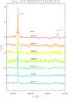 |
Fig. A.10 Same as Fig. 16, but for V371 Tau. |
| In the text | |
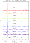 |
Fig. A.11 Same as Fig. 16, but for V343 Tau. |
| In the text | |
Current usage metrics show cumulative count of Article Views (full-text article views including HTML views, PDF and ePub downloads, according to the available data) and Abstracts Views on Vision4Press platform.
Data correspond to usage on the plateform after 2015. The current usage metrics is available 48-96 hours after online publication and is updated daily on week days.
Initial download of the metrics may take a while.