| Issue |
A&A
Volume 664, August 2022
|
|
|---|---|---|
| Article Number | A78 | |
| Number of page(s) | 30 | |
| Section | Catalogs and data | |
| DOI | https://doi.org/10.1051/0004-6361/202243268 | |
| Published online | 11 August 2022 | |
Characterization of Kepler targets based on medium-resolution LAMOST spectra analyzed with ROTFIT★,★★
1
INAF - Osservatorio Astrofisico di Catania,
via S. Sofia, 78,
95123
Catania, Italy
e-mail: afrasca@oact.inaf.it
2
University of Wrocław, Faculty of Physics and Astronomy, Astronomical Institute,
ul. Kopernika 11,
51-622
Wrocław, Poland
3
Royal observatory of Belgium,
Ringlaan 3,
1180
Brussel, Belgium
4
Department of Astronomy, Beijing Normal University,
Beijing,
100875
PR China
5
Key Lab for Optical Astronomy, National Astronomical Observatories, Chinese Academy of Sciences,
Beijing,
100101
PR China
Received:
4
February
2022
Accepted:
24
April
2022
Aims. In this work we present the results of our analysis of 16 300 medium-resolution LAMOST spectra of late-type stars in the Kepler field with the aim of determining the stellar parameters, activity level, lithium atmospheric content, and binarity.
Methods. We have used a version of the code rotfit specifically developed for the lamost medium-resolution spectra to determine stellar parameters via the adoption of a grid of spectra of real stars. We provide a catalog with the atmospheric parameters (Teff, log g, and [Fe/H]), radial velocity (RV), and projected rotation velocity (v sin i). For cool stars (Teff ≤ 6500 K), we also calculated the Ha and Li iλ6708 equivalent width, which are important indicators of chromospheric activity and evolutionary stage, respectively.
Results. From the sample of 16 300 spectra, we have derived the RV and atmospheric parameters for 14 300 spectra of 7443 stars. Literature data (mainly from high- or medium-resolution spectra) were used for a quality control of the results and to assess the accuracy of the derived parameters. The Teff and log g values are in good agreement with the literature, although their distribution displays some clustering effects, which may be the result of the nonuniform distribution of the templates in the parameter space. The most relevant differences are found for [Fe/H], which appears to be overestimated for metal-poor stars; this overestimation is also likely due to the template grid. We propose a relation to correct the [Fe/H] values derived with rotfit. We were able to identify interesting objects, such as double-lined binaries, stars with variable RVs, lithium-rich giants, and emission-line objects. Based on the Hα flux, we found 327 active stars. We were able to detect the Li iλ6708 line and measure its equivalent width for 1657 stars, both giants and stars on the main sequence. Regarding the latter, we performed a discrete age classification based on the atmospheric lithium abundance and the upper envelopes of a few open clusters. Among the giants, we found 195 Li-rich stars, 161 of which are reported here for the first time. No relationship is found between stellar rotation and lithium abundance, which allows us to rule out merger scenarios as the predominant explanation of the enrichment of Li in our sample. The fraction of Li-rich giants, ≈ 4%, is higher than expected.
Key words: surveys / techniques: spectroscopic / stars: activity / binaries: spectroscopic / stars: fundamental parameters / stars: abundances
Full Tables C.2, C.3, 2, 3, and 4 are only available at the CDS via anonymous ftp to cdsarc.u-strasbg.fr (130.79.128.5) or via http://cdsarc.u-strasbg.fr/viz-bin/cat/J/A+A/664/A78
© A. Frasca et al. 2022
 Open Access article, published by EDP Sciences, under the terms of the Creative Commons Attribution License (https://creativecommons.org/licenses/by/4.0), which permits unrestricted use, distribution, and reproduction in any medium, provided the original work is properly cited.
This article is published in open access under the Subscribe-to-Open model. Subscribe to A&A to support open access publication.
1 Introduction
The Large Sky Area Multi-Object Fiber Spectroscopic Telescope (LAMOST; Cui et al. 2012) is a National Major Scientific Project undertaken by the Chinese Academy of Science. It is a unique instrument, located at the Xinglong station and situated south of the main peak of the Yanshan mountains in Hebei province (China). LAMOST combines a large aperture (4-meter telescope) with a wide field of view (circular region with a diameter of 5 degrees on the sky) that is covered by 4000 optical fibers. These fibers are connected to 16 multi-object optical spectrometers with 250 fibers each (Wang et al. 1996; Xing et al. 1998), making this instrument the ideal tool for obtaining spectroscopic observations for a large number of targets in an efficient way. The data acquired with the LAMOST instrument allow multi-fold analyses of the observed objects to be conducted, including a homogeneous determination of the atmospheric parameters (APs): the effective temperature Teff, surface gravity log g, metallicity [Fe/H], radial velocity RV, and projected rotational velocity v sin i.
The LAMOST Extra-GAlactic Survey (LEGAS) and the LAMOST Experiment for Galactic Understanding and Exploration (LEGUE) were the two initial scientific driving forces behind the LAMOST project (Zhao et al. 2012). However, it was soon realized that observations of the field of view of the nominal Kepler mission with LAMOST would be a scientific gold mine, being a win-win opportunity for both communities: it would provide the Kepler community with the data needed for a homogeneous spectroscopic determination of stellar parameters for objects observed by Kepler while the LAMOST community could benefit from high-precision results derived from data obtained elsewhere for Kepler objects to calibrate the LAMOST results. Therefore, the proposal of the LAMOST-Kepler project (hereafter LK project) was well received in 2010. A detailed description is given by De Cat et al. (2015, hereafter Paper I). The first observations for the project were carried out during the test phase of LAMOST in early 2011. The scientific observations of the pilot survey of LAMOST began on October 24, 2011, while the first 5-year regular survey started about one year later, on September 28, 2012. During the first regular survey of LAMOST, only single-shot low-resolution spectra (LRS) with a spectral resolution R ~ 1800 covering optical wavelengths ranging from 370 to 900 nm were gathered.
The purpose of the observations collected during the LK-LRS project is multifarious. First, the APs yielded by the LK project complement and can serve as a test bench for the content of the Kepler Input Catalog (KIC; Brown et al. 2011). As such, they provide firm bases for asteroseismic and evolutionary modeling of stars in the Kepler field. Second, the gathered data enable us to flag interesting objects as they allow us to identify fast-rotating stars and objects for which the variability in radial velocity (RV) exceeds ~20 km s−1; such objects are good candidates for spectroscopic binaries or pulsating stars. Similarly, stars that show strong emission in their spectral lines or display other relevant spectral features can be identified and used for further research that reaches beyond asteroseismic analysis. The analysis of the LK LRS has been performed by three teams with different methodologies. Their results have been presented by Ren et al. (2016) and Zong et al. (2018) for the Asian group, Frasca et al. (2016) for the European group, and Gray et al. (2016) for the American group.
In 2015, the LK project was extended to include targets within the fields observed by the K2 space mission (Wang et al. 2020a). Since the start of the second phase of the regular survey of LAMOST in September 2018, medium-resolution spectro-graphs both in single-shot and time-series mode have also been used. The corresponding medium-resolution spectra (MRS) have a spectral resolution R ~ 7500.
Within the LK-MRS project, time series of MRS LAMOST spectra are being gathered for 4 footprints in the Kepler field and 16 footprints distributed within the northern K2 campaigns. Zong et al. (2020) present the first results of the LK-MRS project based on the analysis of the data up to June 2019, with the LAMOST stellar parameter pipeline (LASP) adapted to the resolution of the MRS, R ~ 7500 (Luo et al. 2015; Wang et al. 2019).
In this paper we focus on the MRS of objects in the Kepler field that were gathered during the test phase of the medium-resolution spectrographs in the year between the end of the first and the start of the second regular survey of LAMOST (September 2017–May 2018). They were made available to the general public in the sixth data release (DR6) of LAMOST on September 30, 2020. We adapted the code ROTFIT, developed by Frasca et al. (2003, 2006) and discussed in detail by Molenda-Żakowicz et al. (2013), to MRS LAMOST spectra. Then we applied it to the spectra collected with plates that intersect with the Kepler field of view (both from the LK-MRS project and the regular survey), selecting spectra of sufficient quality to derive the Teff, log g, [Fe/H], RV, and v sin i of the observed stars. Moreover, we determined the residual equivalent width of the Balmer Hα line  to search for active stars, and the equivalent width of the Li I λ6708 Å absorption line WLi to detect young stars.
This paper is organized as follows. In Sect. 2, we briefly describe the selection of our sample and the observations. Section 3 presents the methods of analysis and discusses the accuracy of the data. That section also includes a brief description of the ROTFIT pipeline, the procedure for the measure of the activity indicators, and a comparison of the RVs and APs derived in this work with values from the literature. The results from the chromospheric activity indicators and the lithium abundance, as well as some examples of spectroscopic binaries, are presented in Sect. 4. We summarize the main findings of this work in Sect. 5.
Overview of the LK–MRS plates observed in the period September 2017–June 2018 that have objects in common with the Kepler field.
2 Observations and Sample Selection
The time in between the first (September 2012–June 2017) and second (September 2018–June 2023) phase of the regular survey of LAMOST was used to test new medium-resolution spectro-graphs. They have a spectral resolution of R ~ 7500, covering wavelengths of the visible spectrum ranging from 495 to 535 nm and from 630 to 680 nm with a blue and red arm, respectively (Liu et al. 2019). In this paper, we use MRS retrieved from DR6 that were collected in the above mentioned test phases from plates that have objects in common with the Kepler field. This led to an initial sample of 22,629 MRS LAMOST spectra (Table 1). Their position on the sky is visualized in Fig. 1. Only seven medium-resolution spectrographs were available for the observations in 2017. They were fed by fibers positioned as displayed by the dark blue areas in Fig. 1. LAMOST was fully equipped with 16 medium-resolution spectrographs by the time the observation in 2018 were done (light blue area in Fig. 1). The results of the LASP pipeline (Luo et al. 2015; Wang et al. 2019) and of the convolutional neural network method (Wang et al. 2020b) are given in the LAMOST MRS Parameter Catalog of DR6, which can be downloaded from http://dr6.lamost.org.
In this paper, we used the ROTFIT code (see Sect. 3) for the determination of the stellar parameters, radial and projected rotational velocity (v sin i), chromospheric activity indicators and lithium abundance. We note that APs were already provided for most targets in other works based on different codes (e.g., Zong et al. 2020). For this task we used the stacked MRS, which are the sum of all the individual spectra of the same object acquired in the same night. We decided to analyze these data with our code with the aim to have homogeneously determined parameters, using both the blue- and red-arm spectra, for all the FGKM-type stars for which we derive other parameters of interest, such as the v sin i, Hα emission, and lithium abundance. Since ROTFIT is optimized for cool stars, we selected the spectra to be analyzed based on the results of the LASP pipeline. We subdivided the initial sample into a “hot” sample ( ), a “cool” sample (
 ), and an “unclass” sample (no
  available), which contain 976, 14264, and 7389 spectra, respectively (see “Number of targets” in Table 1). The spectra in the hot sample are not considered in the present work and will be included in a forthcoming paper (Catanzaro et al., in preparation), which will present a customized analysis based on a spectral-synthesis approach. A quick-look analysis of the spectra in the cool and unclass samples allowed us to discard bad spectra (e.g., missing parts or too many strong spikes) and those with clear signatures of hot (A-type or earlier) stars. This selection resulted in about 14250 and 2050 spectra for the cool and unclass sample, respectively. We used a signal-to-noise ratio (S/N) ≥ 10 in at least one arm as a threshold to select the reliable parameters from the cool sample. The success rate for this sample of spectra was very high, as we could determine parameters for 13 630 and 13 793 red- and blue-arm spectra, respectively. However, the unclass spectra with S/N ≥ 10 are only a small fraction of the selected sample (about 200 and 1200 spectra for the blue and the red arm, respectively). Therefore, after a visual scrutiny, we decided to consider also the results from spectra with a S/N as low as 5 in one of the arms for the unclass sample, because no stellar parameters are available yet for these data. We ended up with 692 and 618 unclass spectra with APs in the red and blue arm, respectively. The whole sample selected for a detailed analysis, which includes both cool and unclass, consists of 16300 MRS LAMOST spectra. For 14 300 of these spectra we were able to determine the APs.
The cross-identification with Kepler sources was based on the fiber coordinates, adopting a radius of 3.7 arcsec (cf., Zong et al. 2020; Wang et al. 2020a).
 |
Fig. 1 Selection of the DR6 LK-MRS project data in the Kepler field. The stars observed on plates that have overlap with the Kepler CCDs are shown as dots (blue for stars on a Kepler CCD, dark blue for observations in 2017, and light blue for observations in 2018). |
3 Data Analysis
3.1 Radial Velocity, Projected Rotation Velocity, and Atmospheric Parameters
We measured the RV, the projected rotation velocity, v sin i, and derived the APs − Teff, log g, and [Fe/H] – by applying the code ROTFIT (e.g., Frasca et al. 2006, 2015), which was purposely modified to fit with the LAMOST MRS. We adopted, as templates, a grid of high-resolution spectra of slowly rotating stars (v sin i ≤ 3 km s−1) with a low activity level that were retrieved from the ELODIE archive (R ≃ 42000; Moultaka et al. 2004). This is the same grid as that used for the analysis of young stars within the Gaia-ESO survey by the OACT (Osservatorio Astrofísico di Catania) node (Frasca et al. 2015). It contains spectra of 388 different stars, which sufficiently cover the space of the APs, although the density of templates is not uniform especially in the regime of metal-poor stars.
We prefer real-star spectra over synthetic ones because the former reproduce the unknown photospheric spectrum better, which can be subtracted from the target one to leave the chromospheric core contribution and to clean the Li I line from blended neighbor lines. Some photospheric lines may be missing in the synthetic spectra, or the depths and widths of some of them may be poorly reproduced due to uncertain intensity values, Landé factors and broadening effects.
The first step of the analysis performed by ROTFIT is the normalization of the LAMOST spectra to the local continuum, which was accomplished by the fit of a low-order polynomial. After the normalization, the RV was measured by cross-correlating the target spectrum with spectra of four stars of different spectral type (SpT) selected from the library of ELODIE templates. In particular, we considered HD 117176, HD 166620, HD 95735, and HD 25329, whose SpTs are G5V, K2V, M2V, and K1 metal-poor, respectively. For measuring RV, we chose the cross-correlation function (CCF) with the highest peak, which is the one obtained with the best-matching template. This task was executed both for the blue and red arm of each spectrum, after excluding the lithium line and the core of the Hα line (± 1 Å around the line center), which would broaden the CCF peak and could be contaminated by chromospheric activity. To measure the centroid and full width at half maximum of the CCF peak, we fitted it with a Gaussian. The RV error, σRV, was estimated as the error of the center of the Gaussian fitted to the CCF peak using the procedure CURVEFIT (Bevington et al. 1993), taking the CCF noise, σCCF, into account. The CCF noise was evaluated as the standard deviation of the CCF values in two windows of about 600 km s−1 each at the two sides of the peak. We adopted the value  as the instrumental weight for all the points of the CCF peak that were considered for the Gaussian fit. For the spectra with S /N ≥ 50 we find median RV errors of ≈0.65 km s−1 for the blue-arm and ≈0.70 km s−1 for the red-arm, respectively (see Fig. 2). Although for a small fraction of sources (≈3%) the RV error is σRV > 3 km s−1, the median values reach a maximum of about 1.3 km s−1 for the spectra with a low S/N (S/N < 10). The RV errors in the blue arm display a two-fold behavior, with a larger fraction of them being similar to those of the red arm and barely visible under the red points in Fig. 2 and a second branch with larger values. This double-peaked distribution for the RV errors in the blue arm is clearly visible in the right panel of Fig. 2, where the histogram displays two distinct peaks at about 0.7 and 1.1 km s−1. The peak with RV errors around 1.1 km s−1 corresponds to stars with Teff ≤ 5500 K, for which the spectral features included in this range broaden, giving rise to larger RV errors. We note that the RV errors evaluated with ROTFIT are in agreement with Liu et al. (2019) and Zhang et al. (2021), who report typical values of about 1 km s−1 at S/N = 20. As a further check of the RV errors, we used the task FXCOR of the IRAF1 package and a set of synthetic templates for a small subsample of about 100 LAMOST MRS of FGK-type stars. We find an excellent agreement between the RV values derived with both codes, both for the blue- and red-arm spectra. The errors calculated by fxcor on the basis of the CCF peak’s height and the antisymmetric noise (Tonry & Davis 1979) are, on average, similar to those derived with ROTFIT.
As pointed out by Wang et al. (2019) and Zong et al. (2020), the RV measured on LAMOST MRS can be affected by systematic offsets in different runs that are related to the wavelength calibration. The largest offset of about 6.5 km s−1 is found for spectra acquired before May 2018 that were calibrated with Sc lamps, compared to the following ones for which Th-Ar lamps have been used. To account for these offsets and correct the RVs, we used a method similar to that adopted by Zong et al. (2020), which is based on the RV measured by Gaia for a subset of stars with non-variable RVs enclosed in the LAMOST-MRS plates. For each plate and observing date, these RV differences display a regular distribution that can be fitted with a Gaussian, whose center is a measure of the instrumental offset for the given plate and date (see Figs. C.3 and C.4 for some examples). These corrections are reported in Table C.1.
The resulting RV and σRV values are given in Cols. 16 and 17 of Table C.2 and Table C.3 for the red-arm and blue-arm spectra, respectively. The RVs corrected for instrumental offsets are reported in Col. 18 of the same tables.
For some spectra we noted two or three CCF peaks at a level larger than 5σCCF that we considered as significant (see Fig. 18 for an example). In these cases, we classified the object as a double-lined spectroscopic binary (SB2) or a triple system (SB3), respectively, and flagged its spectra accordingly in Table C.2 and Table C.3. For these systems we discarded the RVs and APs from the above tables, even if they were obtained near the conjunctions, when the lines of the two components are superimposed. The way the RVs of the components of SB2 systems are derived is described in Sect. 4.4.
For the determination of APs, the reference spectra were first aligned onto the target spectrum thanks to the RV measured as described above and were brought to the resolution of the LAMOST MRS, Rmrs ≃ 7500, by convolving them with a Gaussian kernel of width  . Then, each template was broadened by the convolution with a rotational profile of increasing v sin i (in steps of 1 km s−1) until a minimum χ2 was attained.
We point out that the resolution and sampling of the MRS LAMOST spectra do not allow us to measure v sin i values smaller than 8 km s−1. This threshold was found by means of Monte Carlo simulations with artificially broadened spectra that are described in Appendix A. Therefore, the v sin i values smaller than 8 km s−1 in Table C.2 and Table C.3 must be regarded as “non-detection.” Whenever the mean v sin i value is smaller than 8 km s−1 in at least one arm, the final v sin i has been replaced with “< 8 km s−1” and flagged as an upper limit in the table containing the average APs (Table 2).
As mentioned above, for each target we applied ROTFIT on both the blue- and red-arm spectra that were analyzed independently. The templates were sorted in a decreasing order of χ2, giving the highest score to the best-fitting template. The MK SpT of the template with the highest score was assigned to the target star. Two examples of the application of ROTFIT for slowly rotating stars of mid-F and K0 III SpTs are shown in Figs. 3 and Figs. C.1, respectively. An example of the application of ROTFIT for a rapidly rotating (v sin i ≃ 110 km s−1) F5 V star is shown in Fig. C.2.
For each arm, we derived the values of Teff, log g, [Fe/H], and v sin i as the weighted averages of the parameters of the ten best-matching templates, using 1/χ2 as the weight. As uncertainties of these parameters we took the standard errors of the weighted means to which we added in quadrature the average uncertainties of the APs of the templates  , σlog g = ± 0.1 dex, σ[Fe/H] = ± 0.1 dex). For the v sin i, we added in quadrature a value of σv sin i = ± 3 km s−1, to take the uncertainty related to the spectra sampling into account.
As mentioned in Sect. 2, we were able to determine APs and RVs for 97% of the blue-arm spectra in the cool sample, while only 30% of the spectra in the unclass sample could be successfully analyzed. Regarding the red arm, we could measure stellar parameters for 96% of the spectra in the cool sample, and 34% of the unclass-sample spectra. The S/N ranges from 10 to 900 for the analyzed spectra in the cool sample and from about 5 to 450 in the unclass one. However, the median S/N is much smaller in the latter sample, and this explains the lower success rate in determining the parameters. We remark that the samples of stars with parameters in the red and blue arm are not the same. In particular, for the cool and faint stars, the S/N in the red-arm can be sufficient to derive reliable parameters, while it is too low in the blue arm.
The errors of v sin i, Teff, log g, and [Fe/H] are displayed as a function of S/N in Fig. 2. As shown in this figure, the v sin i errors range from about 3 to 10 km s−1, with median values rising to about 4 and 5 km s−1 for the blue and red arm, respectively, at the lowest S/Ns. The scatter plot for the percent error of Teff shows values ranging from about 1% to 9%, with an increasing trend for decreasing S/N. The median values of about 2% and 2.5% for the blue and red arm, respectively, increase slightly with the decrease of S/N. The errors of log g are smaller than 0.5 dex for nearly all the spectra, with median values of about 0.20 and 0.25 dex for the blue and red arm, respectively. The log g errors increase slightly with the decrease of S/N, as shown by the scatter plot and the median, with the red-arm ones being larger, as also indicated by higher tail of the red histogram. [Fe/H] values have uncertainties smaller than 0.3 dex for most of the spectra, with median values of 0.15 dex for both the blue and the red arm. As for Teff and log g, the [Fe/H] errors increase slightly with the decrease of S/N; this effect is larger for the red-arm values, as also shown by the histograms.
We remark that stellar parameters obtained from both arms are consistent for the vast majority of the stars contained in our sample (see Fig. 4). If we compare the RVs measured by us in the blue and red arm, which are simultaneous, we find an offset of about −0.1 km s−1 between blue and red RVs and an rms dispersion of 2.3 km s−1 (see Fig. C.5). This can provide us with a further estimate of the average RV accuracy. If we assume that the blue- and red-arm RVs have, on average, the same uncertainty, we should divide this number by  , getting an estimate of about 1.6 km s−1 for the RV accuracy in both arms. On average, we find differences (blue arm minus red arm) of: ∆ Teff = 65 ± 175 K, ∆ log g = −0.08 ± 0.26, ∆[Fe/H] = 0.00 ± 0.12 and ∆v sin i = −8.7 ± 9.5 km s−1. For the v sin i, the differences are ∆v sin i = −3.8 ± 3.4 km s−1, if we exclude the upper limits. For a better display of the results, the distribution of these differences for each parameter, taking the red arm as a reference, is shown in Fig. 5. As seen above for the RV, the difference between the APs in the blue and red arm enables us to estimate average uncertainties, which turn out to be (dividing by
  ) about 120 K, 0.18 dex, 0.09 dex, and 2.5 km s−1 for Teff, log g, [Fe/H], and v sin i, respectively. The “zigzag” pattern shown by the Teff and log g plots in Fig. 4, which is more evident in Fig. 5, is the effect of the clustering of the average parameters around those of the best (minimum χ2) template. This is not surprising, because, unlike other analysis codes, ROTFIT does not apply any kind of interpolation or regularization between the parameters of the closest templates. We note the floor of low v sin i values for the blue-arm spectra (v sin iBLUE), which extends up to v sin iRED = 50−60 km s−1 and translates into the tilted strip in Fig. 5. This indicates cases in which the red arm provided a poor constrain to v sin i due to the few absorption lines or to the presence of molecular bands in their red-arm spectra.
The final APs were obtained as the weighted mean of those of the two arms, whenever measures in both arms were available. As described in Sect. 2, in total (from the cool and unclass samples) we selected about 16 300 spectra for our analysis. These spectra, once their coordinates were cross-matched, correspond to 8268 different stars. For 825 of such sources, it was not possible to find reliable parameters because of the binary nature of some sources (see Sect. 4.4) or due to the poor quality of the spectra in other cases. In total, we provide parameters (see Table 2) for 7443 stars, the vast majority of which (7146 stars) has been obtained from both arms. Most of the stars were observed only once (5487) while the rest (1956) have been observed up to six times.
The final parameters (i.e., the average values for each star obtained from all its individual measurements) were calculated by employing a S/N-weighted mean, while the uncertainties were quantified by using the average of individual errors. For the stars observed once, with both arms we averaged both values, whereas for those stars with multiple observations we first calculated a single value per arm and then performed the average of both. We remark that the average value of the RV for stars with multiple observations can hide a genuine RV variation ascribable to pulsations or to the presence of an unseen close companion that would make the source a single-lined spectroscopic binary (SB1). Therefore, we do not list this value in Table 2, but, for stars with multiple observations, we calculated the reduced χ2 and the probability P(χ2) that the RV variations have a random occurrence (e.g., Press et al. 1992). Whenever P(χ2) < 0.05 we considered the RV variation as significant and flagged the corresponding source with “RVvar” in Table 2. However, the individual values of RV measured in each spectrum can be found in Table C.3 and Table C.2 for the blue and red arm, respectively. In general, the APs derived from different arms or observations are in good agreement with each other. Just a few outliers have been detected. In these cases, a visual check of the spectra helped us to improve the results by leaving out the worst ones (i.e., the noisiest, those with artifacts, etc.).
Also, Gaia parallaxes have been used to discern the proper values when large discrepancies in log g-values were found. This was particularly helpful for low-signal spectra of M-type stars. Typical errors from different arms or observations are one or two spectral subtypes. Lastly, the final S/N was taken as the average of individual values. This number is not intended to be an actual ratio but only an indication of the overall quality of the spectra for each target. These final values (Teff, log g, [Fe/H], v sin i, SpT and S/N) are displayed in Table 2 for the stars in our sample along with their equatorial coordinates, KIC designation, number of observations (N) and an indication of the arm(s) with which they have been observed (Arm): blue (b), red (r) or both (br). The last column (Rem) reports any useful remark, such as RVvar for stars with variable RV, Li for stars with a detection of the Li I λ6708 absorption line, and Haf or Hae for stars with the Hα line filled in by core emission or with a pure Hα emission profile above the local continuum.
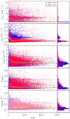 |
Fig. 2 Errors of v sin i, RV, Teff, log g, and [Fe/H] (from top to bottom) as a function of the S/N for the blue-arm and red-arm spectra. The full cyan and yellow lines in each box are the median of the blue-arm and red-arm errors, respectively. The blue and red histograms in the right panels display the distributions of these errors for the blue-arm and redarm spectra, respectively. |
Final APs of the investigated sources.
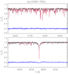 |
Fig. 3 Example of the continuum-normalized LAMOST spectrum of a slowly rotating mid-F star (dots) in the blue arm (upper panel) and in the red arm (lower panel). The best template found by ROTFIT is overplotted with a thin red line. The difference between the two spectra is shown in the bottom of each panel with a blue line shifted upward by 0.2. |
 |
Fig. 4 Comparison of the parameters obtained from both arms. Typical errors are displayed in the bottom-right corner of each panel. In the panel corresponding to the v sin i, the dashed lines show the upper limit at 8 km s−1. |
 |
Fig. 5 Differences obtained from both arms (blue and red) for each parameter. In the panel corresponding to the v sin i, the dashed line shows the upper limit at 8 km s−1. |
 |
Fig. 6 Comparison with the APOGEE RVs. Upper-left panel: comparison between the RV measured on the blue-arm LAMOST MRS (Table C.3) and APOGEE values (Jönsson et al. 2020). Filled symbols represent the stars with multiple spectra. The one-to-one relation is shown by the continuous line. The RV differences between LAMOST and APOGEE, ∆RV, are displayed in the lower box and show an average value of 0.0 km s−1 (dashed line) and a standard deviation of 6.1 km s−1 (dotted lines). Upper-right panel: same as the upper-left panel but for the red-arm RVs listed in Table C.2. The purple squares in both panels enclose the more discrepant points (more than four times the rms). The distributions of the RV differences are shown by the histograms in the lower panels. The Gaussian fits are overplotted with black lines, and the center (μ) and dispersion (σ) of the Gaussians are also marked in these boxes. |
3.2 Comparison with the Literature
The uncertainties evaluated by ROTFIT (Sect. 3.1) are internal to the procedure and do not give an account of the real accuracy of the parameters. To this aim we compared the parameters that were derived in the present work with those available in the literature. As regards the RV, we compared the values measured in the blue-arm and red-arm spectra (Fig. 6), corrected for the systematic offsets, with those measured by the Apache Point Observatory Galactic Evolution Experiment (APOGEE) and reported in the DR16 catalog (Jönsson et al. 2020). We note an almost zero average offset between our corrected RVs and APOGEE, both for the blue and red arm. The rms of the data dispersion around the mean is 6.1 km s−1 for both arms, which can be considered as an upper limit for the data accuracy. Indeed, some stars can have variable RVs because of pulsations or due to the presence of an unseen companion. The points that are more discrepant in Fig. 6 refer to 18 stars (KIC 5268955, 5527172, 5609753, 5688032, 6425135, 6777016, 6924881, 7119181, 7879399, 8022670, 8223328, 8687869, 9099927, 9651996, 10294429, 10987439, 11044668, and 11554998) that are known to be variable in RV in previous studies (see Frasca et al. 2016; Luo et al. 2016, 2018; Wang et al. 2019, 2020b; Jönsson et al. 2020; Tian et al. 2020) or show a significant RV spread in the MRS analyzed in this work. If we discard these data the rms scatter decreases to 3.4 km s−1. Another way to see the effect of stars with variable RV and to take it into account, is to investigate the distributions of the RV differences between LAMOST and APOGEE, which we have plotted in the lower panels of Fig. 6. The distributions, both for the red and the blue arm, are regular and symmetrical in their central part, which has been fitted with a Gaussian. The excesses with respect to the Gaussian in the wings of the distributions are most likely due to objects with variable RV. The Gaussian fits suggest an accuracy of the RV measurement of about 1.3 km s−1 or better.
The results of the comparison of the APs derived from MRS in the present work with those found in the literature are shown in Figs. 7, 8, and 9 for Teff, log g, and [Fe/H], respectively. The majority of the literature parameters that are used for those comparisons were derived with the APOGEE Stellar Parameter and Chemical Abundance Pipeline (ASPCAP) for 2486 stars from the APOGEE DR16 catalog (Jönsson et al. 2020) and with LASP adapted to the MRS (see Zong et al. 2020, and references therein) for 2408 stars. The values of the APs determined by us are plotted versus the APOGEE ones in the middle panels of Figs. 7, 8, and 9, while the comparison with the LASP ones is shown in the bottom panels of the same figures. The remaining literature determinations, which are compared with our values in Figs. 7a, 8a, and 9a, were derived from high-resolution optical or, in two cases, low-resolution infrared spectra by Brewer & Fischer (2018, 48 stars, navy blue circles), Brewer et al. (2016, 19 stars, green diamonds), Furlan et al. (2018, 127 stars, green circles), Grieves et al. (2018, 34 stars, red circles), Guo et al. (2017, 63 stars, azure circles), Huber et al. (2014, 86 stars, orange circles), Lomaeva et al. (2019, 7 stars, yellow squares), Niemczura et al. (2015, 2 stars, yellow triangles), Niemczura et al. (2017, 2 stars, yellow triangles), Notsu et al. (2015, 1 star, yellow triangle), Petigura et al. (2017, 51 stars, yellow circles), Sarmento et al. (2020, 62 stars, black pentagons), or Tkachenko et al. (2013, 1 star, yellow triangle).
Those 5397 determinations concern 4018 individual stars. For 2892 stars from that sample, the literature values of APs were provided only in one paper, for 980 stars in two papers, for 90 stars in three papers, for 30 stars in four papers, for 12 stars in five papers, for seven stars in six papers, for three stars in seven papers, and for four stars in eight papers. Since the above mentioned works do not provide information on all the three APs, the numbers of individual stars for which we found the literature values of Teff, log g and [Fe/H] are, respectively, 5220, 3994, and 5179.
In order to find a linear relation between our determinations of the APs and the literature values, for each star we either used the literature values of the APs and their errors (stars with single literature determinations) or computed the weighted means of the APs and their errors (stars with two or more literature determinations). We note the overall good agreement between our Teff values and those from the literature, with an average offset of only 5 K and an rms of 160 K. Indeed, a linear regression (full line in Fig. 7a) gives a slope b = 0.89, which is smaller than one-to-one relation (dotted line in the same plot). A similar slope is seen in Fig. 7c in which we compare our Teff values with those derived with the LASP pipeline. However, the agreement with the APOGEE temperatures, shown in the middle panel, looks better and the linear regression has a slope nearly equal to 1 (b = 0.98). “The dispersion of the Teff differences around the mean is of about 160 K, which is an estimate of the accuracy of our Teff determinations. In Fig. 7c, there are two Teff outliers, which we (discuss in more detail in Appendix B.
The values of log g display also a good agreement with the literature with a small offset of only 0.01 dex and a scatter of about 0.31 dex (Fig. 8 a). The comparison of our values of log g with those from APOGEE and LASP catalogs (Fig. 8b and Figs. 8c, respectively) displays an overall good agreement, with an rms dispersion of ≈0.3. We note only very few discrepant sources that are labeled with their KIC identifiers and discussed in Appendix B.
The agreement of log g with the literature is better than that found in Frasca et al. (2016, hereafter Paper II), where we found most of the log g values derived from low-resolution LAMOST spectra to be clustered around the gravity typical for red giants (log g ≈ 2.5) and main-sequence (MS) stars (log g ≈ 4.5). The clustering effect, which is mostly the result of the nonuniform density of templates in the space of parameters, is less pronounced in this case, likely due to the higher sensitivity to log g of spectra with a higher resolution. That effect is still visible for the data in the present work, especially for the stars with low gravity for which the ROTFIT values tend to cluster around log g = 1.5, which is very likely caused by the small number of templates with a very low gravity. However, the comparison presented in this paper shows that the log g values are accurate enough to distinguish between giant and MS stars, which, together with an accurate Teff determination unaffected by interstellar extinction, was one of the main purposes of our analysis. The knowledge of these parameters is, in fact, necessary for the spectral subtraction and flux calibration that we use to measure the chromospheric emission in the Hα core (see Sects. 3.3 and 4.1) and the lithium equivalent width and abundance (Sect. 4.2).
The agreement of [Fe/H] values with the literature is much poorer than of the previous parameters (Fig. 9). We found a very small slope for the linear regression of the data (b = 0.54 in Fig. 9a or b = 0.39 in Fig. 9b), which indicates that we are getting correct [Fe/H] values only around the solar one ([Fe/H] = 0) and we are systematically overestimating the metallicity for metal-poor stars ([Fe/H] < −0.3) and underestimating it for metal-rich stars ([Fe/H] > +0.2). We think that this effect, already seen in the results based on the low-resolution data of PaperII, is due to the relative scarcity of metal-poor and super metal-rich stars among our templates that generates a sort of “smoothing” of the final [Fe/H] values. Indeed, the handful of stars with the lowest metallicity in Fig. 9 a and b lie close to the one-to-one relation. For these stars, the templates with a higher metallicity have a spectrum so different that they have not played any role in the [Fe/H] determination.
We thus propose a correction relation for the LAMOST metallicity, based on the linear fit shown in Fig. 9b, which can be expressed as
![${\left[ {{\rm{Fe/H}}} \right]_{{\rm{corr}}}} = 2.57 \cdot \left[ {{\rm{Fe/H}}} \right] - 0.01,$](/articles/aa/full_html/2022/08/aa43268-22/aa43268-22-eq11.png) (1)
(1)
Additionally, in Fig. 9c we find a group of 27 stars, which have been enclosed in a yellow rectangle. All those stars are cool (Teff ≲ 4500 K) giants for which the LASP [Fe/H] values are very low while the ROTFIT [Fe/H] values are close to zero. Those stars we discuss in more detail in Appendix B.
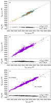 |
Fig. 7 Comparison of Teff values. (a) Comparison between the values of effective temperature in our database of LAMOST spectra and in the literature. Filled symbols represent dwarfs (log gROTFIT ≥ 3.5), open symbols represent giants (log gROTFIT < 3.5). Different colors have been used for different literature sources, as indicated in the main text. The comparison with the APOGEE and LASP Teff is shown in the middle (b) and bottom (c) panels, respectively. The dotted lines in the top box of each panel represent one-to-one relationships. The solid lines are linear fits to the data. The differences between ROTFIT and literature parameters are shown in the lower parts of each panel along with their average values and standard deviations. Stars indicated with arrows are discussed in the text. |
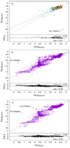 |
Fig. 8 Comparison of log g values derived in the present work with those from the literature (a), APOGEE (b), and LASP (c). The meaning of lines and symbols is as in Fig. 7. |
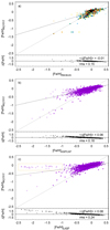 |
Fig. 9 Comparison of [Fe/H] values derived in the present work with those from the literature (a), APOGEE (b), and LASP (c). The meaning of lines and symbols is as in Fig. 7. The sources enclosed in the yellow rectangle in box (c) are discussed in Appendix B. |
3.3 Balmer Hα and Lithium Equivalent Width
The most sensitive diagnostics of magnetic activity in the range covered by the LAMOST MRS is the Balmer Hα line. We therefore identified objects with Hα emission, which can be produced by various physical mechanisms in addition to the presence of an active chromosphere, such as magnetospheric accretion in the youngest evolutionary phases of low- and intermediate-mass stars, or circumstellar (or circumbinary) matter. As the chromospheric emission can only show up as a small to moderate filling of the line core, depending on the activity level and on the photospheric flux of the star, the removal of the photospheric spectrum is crucial to emphasize the Hα core emission. To this aim, we subtracted the non-active template that best matches the final APs from each LAMOST red-arm spectrum. This template has been aligned to the target RV, rotationally broadened at the v sin i of the target and resampled on its spectral points. The “emission” Hα equivalent width,  , was interactively measured by integrating the residual emission profile (see Fig. 10, upper panel).
To speed up this procedure and to reduce spurious detections, we firstly made the measurements of  only on the spectra with a S/N ≥ 20. Moreover, among these spectra, we selected a subsample of likely active stars as those for which an automatic procedure, which measure the Hα equivalent width in a fixed wavelength range of 3 Å around the line center, gave rise to a value larger than 0.1 Å. Then, to pick up low-signal (6 < S/N < 20) spectra with a relevant filling or a pure Hα emission above the continuum, we added the spectra with S/N < 20 for which the “initial” automatic measure of
  was larger than 0.5 Å in the same integration range. For all these spectra, the
  was measured interactively, as described above, and the error was calculated as the product of the integration range times the error in the placement of the continuum, which was evaluated as the rms of the values of the subtracted spectra in two regions at the two sides of the Hα line. We end up with a total of 546+31 (cool,+ unclass) spectra of 334 stars displaying Hα in emission or filled in by a minimum amount as defined above. The maximum value,
  , was found for KIC 8749284, an active star already discovered by us in Paper II as an object with Hα emission above the continuum.
The values of  , along with their errors, are quoted in Table 3. We also report whether the line is observed as a pure emission feature and whether the measure is uncertain as a result of the low S/N or other possible spectral issues.
The subtraction of the photospheric template also allowed us to measure the equivalent width of the Li I λ6707.8 Å line by removing the nearby lines (basically Fe I λ6707.4 Å), which are blended with the lithium line in the observed spectrum. We used a similar approach to that used for Hα to select the spectra on which we measure the lithium equivalent width, WLi. We fixed a threshold of 0.05 Å (50 mÅ) from an automatic measurement of the lithium absorption in the residual spectrum integrating it in a range of 6 Å centered on the Li I λ6707.8 Å line for the spectra with an S/N larger than 20 and 150 mÅ for the low-signal spectra. We detected a WLi above the given thresholds for 2763 spectra, corresponding to 1657 different stars. For stars with multiple visits, we calculated the weighted average of the values of WLi measured in different epochs, adopting a weight  , where
  is the error on the individual measure. We took the maximum of the weighted standard deviation and the standard error of the weighted mean as the final uncertainty.
The highest value of lithium equivalent width, WLi = 626 mÅ, was found for KIC 11657857 (= IRAS 19170+4937), which is also one of the coldest lithium-rich giants ever discovered.
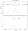 |
Fig. 10 Example of the subtraction of the best non-active, lithium-poor template (red line) from the spectrum of KIC 8095028 (black dots), which reveals the chromospheric emission in the Hα core (blue line in the top panel) and emphasizes the Li I λ6708 Å absorption line, with the nearby blended lines removed (bottom panel). |
Activity indicators.
4 Results
4.1 Chromospheric Activity
Late-type stars, which have convective envelopes, rotation and differential rotation able to produce strong magnetic fields by a dynamo action, display a complex of phenomena known as magnetic activity. These include, radio and/or X-ray coronal emission, UV and optical emission lines produced in a chromosphere, fast energy releases (in the continuum and/or in spectral lines) known as flares, and rotational modulation of brightness produced by cool spots. For stars with a SpT later than mid-F (Teff ≤ 6500 K) the Hα line is an efficient diagnostic of magnetic activity, especially for the cooler ones with a moderate to high level of activity, if we subtract the underlying photospheric spectrum, as we have explained in Sect. 3.3.
The equivalent width of an emission line formed in a chromospheric layer can be used to quantify the activity level, when it is converted into energetic units. Therefore, more accurate indicators of chromospheric activity are the line flux in units of stellar surface, F, and the ratio between the line luminosity and bolometric luminosity, R′, which can be calculated, for the Hα, as
 (2)
(2)
 (3)
(3)
where F6563 is the continuum surface flux at the Hα center, which we evaluated from the BT-Settl synthetic spectra (Allard et al. 2012) at the stellar temperature and surface gravity of the target. The flux error includes both the error of the equivalent width and the uncertainty in the continuum flux at the line center, which is obtained by propagating the Teff and log g errors.
The Hα fluxes and  of our targets are plotted as a function of the effective temperature in Fig. 11 using different symbols for giant (open circles) and MS stars (dots). This plot also shows the boundary between young stars with mass accretion and chromospherically active stars. The latter lie below this line, which is also close to a “saturated” activity regime for MS stars (see, e.g., Frasca et al. 2015).
We note that only two stars lie higher (or right over) the dividing line (3 and 4 in Fig. 11), but we classified them with ROTFIT as giant stars. Their high Hα flux is likely the fingerprint of an extremely high activity level due to an enhanced rotation rate, which could be the result of a particular evolutionary phase or of spin-orbit synchronization for an unresolved binary or an SB1 system in which the companion of the cool giant is overwhelmed by its flux (similar to many long-period RS CVn binaries). We cannot exclude the contribution of other processes, such as circumstellar matter or shells, as the cause for the strong Hα emission (see also their Hα profiles in Fig. C.6).
The stars with the highest Hα flux, which lie above or close to the dividing line between accretors and chromospherically active stars, are indicated with progressive numbers (with decreasing Teff) in Fig. 11. In the following we report a few notes on these sources.
KIC 9720659 (#1) is the star with the earliest SpT (F0V, Teff = 6785 K) in our sample of Hα emitters. According to the Hα profile, it could be a Herbig star, with broad wings typical of an A- or F-type star with an emission core, similar to CQ Tau (e.g., Alcalá et al. 2021, and references therein). We did not detect any other emission line in its spectrum. However, a moderate infrared excess, indicative of circumstellar matter or a protoplanetary disk is visible in its spectral energy distribution (SED; Fig. D.3).
KIC 8022670 = V2279 Cyg (#2) is mentioned in the SIM-BAD astronomical database as an “eruptive variable star.” It has been reported as a periodic variable (Cepheid?) by Schmidt et al. (2007) and Pigulski et al. (2009) with a period of about 4.12 days and an amplitude of 0.30 mag. Schmidt et al. (2011) included this star in their study of type II Cepheid candidates and related stars from the Robotic Optical Transient Search Experiment 1 (ROTSE-1), which was based on LRS. They report Teff in the range 4905−4957 K, log g = 4.1, and a solar metallicity. They also report Hα emission (c.f. their Fig. 1) with a Lick-IDS (Lick Observatory Image Dissector Scanner) index of about −2.29. We find nearly the same effective temperature, Teff = 4985 ± 110 K, but a different log g = 2.64 ± 0.41 dex. The latter is in better agreement with other literature values, such as log g = 2.68 (Christiansen et al. 2012) or log g = 2.82 (Ho et al. 2017) that indicate this star as a giant. It was subsequently reported as an active flaring star by Davenport (2016) and Oláh et al. (2021) on the basis of Kepler photometry. In particular, Oláh et al. (2021) classify it as a flaring giant with a radius of 3.3 R⊙ for which 55 flares have been detected by Kepler.
KIC 8749284 (#3) is reported in SIMBAD as a “rotationally variable star” with a period Prot ≃ 3.22 days (Debosscher et al. 2011). It is also classified as an active giant, based on Kepler light photometry (see Gaulme et al. 2020), which displays intense flare activity (Oláh et al. 2021), with 88 flares detected during Kepler observations. We find Teff = 5048 ± 112 K and log g = 3.20 ± 0.30, which indicates an evolved star, as only a weak lithium absorption line (WLi ≃ 40 mÅ), which is not compatible with a pre-main-sequence (PMS) object, has been detected. This is in agreement with the Teff=5089 K and the radius of 4.6 R⊙ reported by Oláh et al. (2021). The SED of this object reveals a strong infrared excess that begins from the H band, which is likely due to cold circumstellar matter. We note that this star was already included in the LK-LRS project and we already detected the Hα emission in the low-resolution LAMOST spectra as well as the infrared excess in its SED (Frasca et al. 2016).
KIC 6201369 (#4) is not present in SIMBAD. In the Gaia early third data release (EDR3) there is a nearby source at about 6 that is about 6 mag fainter. No spectroscopic observations can be found in the literature for this object. We find Teff = 4731 ± 118 K and log g = 2.76 ± 0.27, meaning that it is likely another active giant with a very strong and redshifted Hα emission. The Li Iλ6708 line is not detected in the MRS spectrum of this source. There is no information in the literature about brightness variations; this source, although in its field of view, was not observed by Kepler.
KIC 8095028 (#5) is a young (strong lithium) fast-rotating (Prot = 0.397 d, McQuillan et al. 2014) and flaring star (see Davenport 2016; Goodarzi et al. 2019). An MRS spectrum of this target is displayed in Fig.10. We classified it as a K3.5V star with Teff=4858 ± 126 K and log g=4.58 ± 0.15, to be compared with the values of Teff = 4464 K and log g = 4.49 reported by McQuillan et al. (2014). The lithium equivalent width of WLi = 272 mÅ places this star just below the Pleiades upper envelope in Fig. 12 (i.e., it is the MS star with the highest WLi in our sample; see Sect. 4.2).
KIC 10063343 (#6) is an ultrafast rotator (Prot = 0.337 d, McQuillan et al. 2014), which shows several flare episodes in the Kepler light curves (see, e.g., Davenport 2016; Yang & Liu 2019). We confirm it as a K5V star (Teff = 4579 ± 105, log g = 4.65 ± 0.11) rotating at v sin i = 104 km s−1. The Li Iλ6708 line is not visible in the low-signal MRS spectrum of this source.
KIC 8935655 (#7) is a dMe flaring star (see Yang et al. 2017; Davenport 2016). Hardegree-Ullman et al. (2019) report an M4V SpT and Teff = 3241K; we find this star slightly earlier (M1.5V) and hotter (Teff = 3575 ± 102 K) and confirm it as a slowing rotating (v sin i < 8 km s−1) dMe star. Our temperature is instead in very good agreement with that based on APOGEE spectra, Teff = 3554 ± 69 K (Jönsson et al. 2020). The Li Iλ6708 line is not visible in the MRS spectrum of this source.
 |
Fig. 11 Activity indicators. Left panel: Hα flux versus Teff (open circles for giants, purple dots for MS stars). Right panel: |
4.2 Lithium Abundance and Age
Lithium is burned in stellar interiors at temperatures of about 2.5 × 10⁶ K. Therefore, it is progressively depleted from the stellar atmospheres of late-type stars with deep enough convective envelopes. The degree of depletion depends on the internal structure of the star and therefore, for the MS stars, on the mass. Thus, its abundance can be used as an empirical indicator of age for MS stars cooler than about 6500 K. A simple and effective way to get an age estimate is a diagram showing the equivalent width of lithium as a function of effective temperature (or a color index) together with the upper envelopes of young open clusters that can be used as boundaries to separate the star sample in age classes (Fig. 12).
We adopted the upper envelopes of the Hyades (Soderblom et al. 1990), the Pleiades (Soderblom et al. 1993a; Neuhaeuser et al. 1997), and IC 2602 (Montes et al. 2001), whose ages are of about 650 (White et al. 2007), 125 (White et al. 2007), and 30 Myr (Stauffer et al. 1997), respectively. The lower envelope of the Pleiades corresponds to the upper boundary for the members of the Ursa Major (UMa) cluster (age ≈ 300 Myr; Soderblom et al. 1993b). The boundaries are remarkably close to each other for temperatures higher than 6000 K and therefore, also taking into account the errors on WLi, we preferred to restrict the age classification to objects with Teff ≤ 6000 K. In line with what done by Guillout et al. (2009) and Frasca et al. (2018), we have defined four age classes for the MS stars: (i) “PMS-like” encompasses objects that lie above the Pleiades upper boundary; (ii) “Pleaides-like” comprises stars that fall between the upper and lower Pleiades envelopes; (iii) “UMa-like” stars are those located between the lower Pleiades boundary (corresponding to the UMa upper envelope) and the Hyades envelope; and (iv) “Hyades-like” stars are those with WLi > 20 mÅ that lie below the Hyades upper envelope.
We adopted a lower threshold of 20 mÅ for the Hyades-like stars, because the typical error of WLi is 20 mÅ, and lower values of WLi are normally associated with stars older than the Hyades. Therefore, the stars with WLi < 20 mÅ and those for which no Li I absorption has been detected are not classified. The stars that belong to the four age classes defined above are labeled as PMS, Ple, UMa, and Hya, respectively, in Table 4. The MS star with the highest value of WLi is KIC 8095028, which is close to the upper envelope of the Pleiades stars. In the end, only three MS stars were classified as PMS-like, but all of them lie very close to the Pleiades upper envelope and therefore their PMS nature is questionable; they should be broadly considered as very young stars. We find 19 Pleiades-like (1.6%), 247 UMa-like (21%), and 343 Hyades-like stars (30%) in our sample of MS stars (log g > 3.7) with a detection of the lithium line (1184 stars).
We calculated the lithium abundance, A(Li), from our values of Teff, log g, and WLi by interpolating the curves of growth of Lind et al. (2009), which span the Teff range 4000–8000 K and log from 1.0 to 5.0 and include nonlocal thermal equilibrium corrections. We note that for the few stars with Teff < 4000 K the lithium abundance is extrapolated and could be less accurate. The errors of A(Li) take into account both the Teff and WLi errors2. In Fig. 13 we show the lithium abundance as a function of Teff along with the upper envelopes of the distributions of some young open clusters shown by Sestito & Randich (2005). We note that the age of NGC 6475 of about 300 Myr is close to the UMa cluster, and its upper envelope corresponds to the lower envelope of the Pleiades in Fig. 12. This plot shows that the age classification made on the basis of the WLi diagram and upper envelopes of open clusters is confirmed by the A(Li) diagram.
The object with the highest lithium abundance, A(Li) = 3.97 ± 0.26, is KIC 11657857 (= IRAS 19170+4937), which is also the coolest lithium-rich giant. The SED (see Sect. 4.3) of this source (Fig. D.1) displays infrared excess starting from about 10 μm, which is clearly revealed by IRAS (Abrahamyan et al. 2015), AKARI (Ishihara et al. 2010), and WISE (Cutri et al. 2021) data. Another object with a very large value of lithium abundance (A(Li) = 2.98 ± 0.15) is KIC 8363443, which is a lithium-rich giant already known from the literature. No infrared excess is visible in the SED of this source (Fig. D.2).
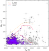 |
Fig. 12 Equivalent width of the Li I λ6707.8 line (WLi) plotted as a function of Teff (open circles for giants, purple dots for MS stars). The lines show the upper boundaries for Hyades (dash-dotted blue), Pleiades (solid red for both the lower and upper boundary), and IC 2602 (dashed orange) clusters. Most of the stars with a strong lithium absorption are lithium-rich giants. |
Lithium equivalent widths and abundances.
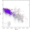 |
Fig. 13 Lithium abundance as a function of Teff. The upper envelopes of A(Li) for IC 2602, Pleiades, NGC 6475 (age ≈ 300 Myr), and Hyades clusters adapted from Sestito & Randich (2005) are overplotted. The meaning of the symbols is the same as in Fig. 12. |
4.3 Lithium-Rich Giants
As mentioned in Sect. 4.2, lithium is a fragile element, which is progressively destroyed by nuclear reactions at temperatures much lower than those of H-burning cores. As such, it is very sensitive to stellar evolution. Canonical models (Iben 1967a,b; Soderblom et al. 1993a) predict Li depletion as a direct consequence of the first dredge-up (FDU) once stars reach the red giant branch (RGB). According to this, we do not expect to find abundances of Li above 1.5 dex in red giants (Charbonnel & Balachandran 2000). Observations confirm this theoretical scenario (Bonsack 1959; Gratton et al. 2004). However, a few giants with Li abundances larger than this value, the so-called Li-rich giants, have been discovered since several decades (e.g., Wallerstein & Sneden 1982; Luck 1982). A large number of such stars have recently been found in the field (Casey et al. 2016; Smiljanic et al. 2018; Gao et al. 2019; Martell et al. 2021), globular clusters (Kirby et al. 2016) as well as open clusters (Monaco et al. 2014; Alonso-Santiago et al. 2017, 2019; Magrini et al. 2021) representing a fraction around 1 % of all known giants. These stars have from early-F to A-type progenitors on the MS (M* = 1.5−2.5 M⊙).
As noted above, we find 1657 stars with a detectable amount of lithium in our sample of 7443 stars, representing about 21% of the total. Excluding 1184 stars with log g > 3.7, which we classified as MS stars, we are left with 473 evolved stars with a detectable Li I λ6708 line. Among them there are the Li-rich giants (A(Li) ≥ 1.5), including those that exhibit an abundance above the primordial value (i.e., A(Li) ≥ 2.7). We refer to this subset as super Li-rich stars. In order to determine their fraction, we first need to know the total number of giants in our sample. To identify them, we plotted the Kiel (Teff–log g) diagram and examined the distribution of the stars in it. In the left panel of Fig. 14 giants clearly stand out from MS stars. As seen, their maximum density is centered at Teff ≈ 4800 K and log g ≈ 2.6. Moving down in the diagram toward the point of maximum density of MS stars, we set the giants boundary at a place approximately equidistant from both points. In this way, stars with Teff ≤ 5750 K and log g ≤ 3.6 will be considered as giants. By taking this criterion into account, we found 3276 giants in our sample, out of which 195 have A(Li) ≥ 1.5, which implies a fraction of Li-rich giants of 6.0%. This number is practically not affected by minor changes to the selection criterion. Surprisingly, this fraction is much higher than ≈1.3%, which is the result obtained by the most recent surveys (Gao et al. 2019; Martell et al. 2021) after analyzing stellar samples much larger than ours. Among the 195 Li-rich giants detected, 34 were already observed by Gao et al. (2019) while the remaining 161 are reported here for the first time.
In order to understand the evolutionary status of these Lirich giants, we placed them on the Hertzsprung-Russell (HR) diagram. For this task, we first calculated their luminosity from the analysis of the SED, as explained in Appendix D. Then, we added the PARSEC evolutionary tracks (Bressan et al. 2012) for a solar metallicity (Z = 0.017) and finally, we marked the base of the RGB and the RGB bump on them. The resulting HR diagram of these sources is shown in Fig. 15. As inferred from their position on the diagram, the vast majority of our sources are low-mass stars with masses in the range 1−3 M⊙.
According to their position in the HR diagram and the loci indicated in Fig. 15, three evolutionary stages can be distinguished. The first one corresponds to the stars located to the left of the green strip. These objects could have not yet reached the RGB3 and their initial lithium is still observable in their atmospheres. Those stars in the diagram placed between both strips are classified as RGBs. Approximately in the middle of this phase, the FDU takes place and drastically depletes the amount of the photospheric Li. As commented before, A(Li) > 1.5 should not be observed in these stars. Some of them, the closest to the green strip, could not yet have undergone the FDU, and therefore, their lithium abundance is explained as in the previous case. Nevertheless, with regard to the remaining stars, the existence of these Li-rich giants implies the additional contribution of a mechanism capable of enhancing the atmospheric lithium content. This is also valid for those stars found after the RGB bump, to the right of the orange strip.
However, a single universal mechanism that can explain this phenomenon as a whole does not seem to exist; there is more likely a mixture of various processes at work. External pollution is one of the scenarios most often claimed to explain it. The extra contribution of Li could be due to both the engulfment of a substellar companion (Siess & Livio 1999; Aguilera-Gómez et al. 2016) and the enrichment of the local interstellar medium caused by the explosion of a nearby supernova (Woosley & Weaver 1995). On the other hand, the internal production via the Cameron-Fowler mechanism (CFM; Cameron & Fowler 1971) would allow these stars to create new Li. However, an extra-mixing process after the FDU is absolutely required in this case. Binarity has also been invoked to solve the Li puzzle, either as an external or internal mechanism. In the first case, the Li-rich giant would be the consequence of the merge of a white dwarf with a red giant in a binary system (Zhang et al. 2020) while in the second one, the tidal spin-up from a binary companion would provide the internal extra-mixing necessary to start the CFM (Casey et al. 2019).
We tested some of these hypotheses by taking advantage of our observations. Firstly, binarity is unlikely to explain the Li enhancement, as no binaries have been found among our sample of Li-rich giants. The scenario of engulfment of a substellar companion or a white dwarf does not match what is observed either. According to it, we would expect enhanced rotational velocities among the Li-rich stars, as a natural consequence of the transfer of angular momentum (Aguilera-Gómez et al. 2016; Privitera et al. 2016). However, in our sample, no significant differences are found with regards to the fraction of fast rotators (as well as the metallicity distribution) between Li-rich and Li-normal giants (Table 5). Additionally, fast rotators4 (v sin i ≥ 10 km s−1) show an average A(Li) = 2.0 ± 0.5, a value fully consistent with that of stars with v sin i < 10 km s−1, A(Li) =1.9 ± 0.4, and a correlation between lithium abundance and stellar rotation is not observed (see Fig. 16), as also found in previous works (e.g., Martell et al. 2021). However, the occurrence of fast rotators seems to be higher among the super Li-rich giants (42.9%) than in the Li-rich sample (29.9%), although the sample is not so large as to have good statistical significance.
Despite the fact that Li-rich giants are observed throughout the entire RGB phase, recent studies (Smiljanic et al. 2018; Deepak & Reddy 2019; Singh et al. 2019; Casey et al. 2019; Kumar & Reddy 2020; Martell et al. 2021) show that their frequency is significantly higher at the red clump. A higher occurrence in a particular evolutionary phase (i.e., during the He-core burning) would therefore imply an internal origin (likely related to the He flash, Kumar & Reddy 2020) as the main responsible for the Li observed. The accurate classification of the Li-rich giants in the different evolutionary stages is beyond the scope of this work. Only for a merely indicative purpose, we assume that the region in the Kiel diagram (right panel in Fig. 14) with the highest density of stars (the sequence with 2.3 ≤ log g ≤ 3.0) corresponds to the red clump. Then, in line with other works (e.g., Martell et al. 2021) super Li-rich giants are more concentrated in this part of the diagram than Li-rich giants (71.4% versus 51.1%, respectively).
Finally, as commented above, KIC 11657857 is the object that exhibits the highest Li abundance, A(Li) = 3.97, in our sample (see Fig. 17). It is a super Li-rich M-type star (see, e.g., Alcalá et al. 2011, for another example), which also shows an infrared excess. According to its location in the HR diagram (the brightest and the coolest), KIC 11657857 is most likely to be an asymptotic giant branch (AGB) star, the only one in our Li-rich sample. High-resolution spectroscopic observations would be necessary to properly characterize this interesting object.
 |
Fig. 14 Kiel (Teff−log g) diagram for the final sample of the stars observed in this work. The left panel shows the stellar density and the right one highlights the position of the Li-rich (1.5 ≤ A(Li) < 2.7) and super Li-rich giants (A(Li) ≥ 2.7). The dashed lines delimit the area populated by giants according to our selection criteria, as explained in the text. |
 |
Fig. 15 Hertzsprung-Russell diagram for all the Li-rich giants. The symbols are color coded by the lithium abundance A(Li). The PARSEC post-MS evolutionary tracks (Bressan et al. 2012) for a metallicity Z = 0.017 are plotted with black lines. The green and orange strips mark the base of the RGB and the RGB bump, respectively. |
Percentages of fast rotators (v sin i ≥ 10 km s−1) and stars with a solar metallicity (i.e., −0.2 ≤ [Fe/H] ≤ +0.2) among the Li-normal and Li-rich giants.
 |
Fig. 16 Abundance of Li as a function of the ν sin i among our Li-rich giant sample. The vertical line shows the limit between slow and fast rotators, while the horizontal one represents the boundary between Li-rich and super Li-rich giants. |
 |
Fig. 17 Spectrum of KIC 11657857 (black line and dots), the star with the highest abundance of Li in our sample, versus that of a Li-normal giant with similar stellar parameters (red line) around the Li line at 6708 Å, whose center is marked with a vertical dashed line. |
4.4 Spectroscopic Binaries
The resolution of the LAMOST MRS is sufficient to detect binary and multiple systems and to study their RV curves for deriving the orbital elements and the physical parameters of the components of these systems (see, e.g., Pan et al. 2020; Wang et al. 2021).
As anticipated in Sect. 3, in some spectra (more than 250) we noted two or three peaks in the CCF that resulted to be significant in comparison with the CCF noise. These objects are SB2 or SB3 systems, respectively. In these cases, the analysis with ROTFIT is meaningless, so we do not report any parameter in Table C.2 and Table C.3 and flag them as SB2 or SB3. In some cases the binary nature is questionable, because the CCF displays only an asymmetric peak (i.e., no clear valley between the peaks is visible) that can be due to both an unresolved SB2 system or starspots. For these spectra we kept the APs in Table C.3 and Table C.2, whenever we considered them as reliable, and flagged them as “SB2?”. In total, we found 27 spectra corresponding to 7 different sources, which display three peaks in the CCF (SB3) and more than 230 spectra corresponding to 98 sources with two peaks in the CCF (SB2). The SB3 and SB2 binaries in our sample of MRS are listed in Table C.4.
For the spectra with multiple peaks in the CCF that are sufficiently resolved, we derived the RV of the individual components by fitting the CCF with multiple Gaussians with an approach similar to that used for single-lined objects. An example of the fitting procedure for an SB2 system is shown in Fig. 18. The RV values for the individual components of the SB3 and SB2 systems listed in Table C.4 are not reported in this paper and will be published in forthcoming works dedicated to the double and multiple systems in our sample.
Whenever an SB2 system is observed near the conjunctions, only one peak is visible in the CCF and the RV, measured with a single Gaussian fit, has to be considered as a “blended” value of the RVs of the two components, which is close to the velocity of the barycenter of the system.
In the following, we show the case of a few systems for which we could build an RV curve, including also data from a few spectra acquired in 2019 (DR7). We used the weighted average of the corrected RVs measured in the red and the blue arm, with a weight inversely proportional to the squares of their errors. We used the stacked spectra to maximize the S/N for binary systems with a period longer than a few days, while the individual spectra acquired during each night have been used for binaries with a short or unknown period. We mention here the cases of the eclipsing binaries KIC 8301013 and KIC 5359678, whose RV curves based on LAMOST MRS data have been studied by Pan et al. (2020) and Wang et al. (2021), respectively. They also presented an in-depth analysis of their Kepler light curves.
Another eclipsing binary with a period Porb ≃ 24.24 days and a very eccentric orbit (e ≃ 0.680) is KIC 7821010. An orbital solution, based on the Kepler light curve and RVs derived from high-resolution HIDES spectra, has been presented by Helminiak et al. (2019). Our RVs of KIC 7821010 are displayed in Fig. 19. We note the very good agreement with the RVs and the orbital solution of Helminiak et al. (2019), which are also displayed in Fig. 19.
We also measured the RVs of the eclipsing binary system KIC 6206751, which has a much smaller orbital period, Porb = 1.2453 days, and a circular orbit (Lee & Park 2018). We note that the RVs of the primary component are in very good agreement with those from Matson et al. (2017), while for the secondary component, which is much less luminous than the primary, the agreement is less good (Fig. 20), but our values are still compatible within the errors.
As a further example, we show the case of KIC 10274200, a non-eclipsing SB2, for which we determined the period and the orbital parameters from our data only (see Fig. 21). We searched for the best orbital period by applying the periodogram analysis (Scargle 1982) to the RVs of the primary and secondary components. Then, we fitted the observed RV curve with the CURVEFIT routine (Bevington et al. 1993) to determine the orbital parameters and their standard errors, which are listed in Table 6. We remark that these are very preliminary estimates and new data are needed to refine the orbital solution. As mentioned above, a more in-depth study of the RVs of binary and multiple systems will be the subject of future works.
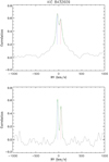 |
Fig. 18 Cross-correlation function (black line) for a double-lined spectroscopic binary (SB2) in the blue arm (upper panel) and in the red arm (lower panel). The two-Gaussian fit of CCF is displayed with a green line, and the centers of the primary (more luminous) and secondary components are indicated with vertical dotted blue and red lines, respectively. |
 |
Fig. 19 Radial velocity curve of KIC 7821010. The RV data from Helminiak et al. (2019) are shown with blue and red squares and the orbital solution with dotted blue and red lines for the primary and secondary component, respectively. The LAMOST MRS RVs derived in this work are overplotted with filled black circles for the primary and open circles for the secondary component, respectively. The green x symbols display the RV values measured by us near the conjunctions, where a single peak is visible in the CCF. |
 |
Fig. 20 Radial velocity curve of KIC 6206751. The RV data from Matson et al. (2017) are displayed with blue and red squares and the orbital solution with dotted blue and red lines for the primary and secondary component, respectively. The LAMOST MRS RVs derived in this work are overplotted with filled black circles for the primary and open black circles for the secondary component. The green x symbols display the RV values measured by us near the conjunctions, where a single peak is visible in the CCF. |
 |
Fig. 21 Radial velocity curve of KIC 10274200. The LAMOST MRS RVs derived in this work are plotted with filled circles for the primary and open circles for the secondary component. The green x symbols display the RV values measured near the conjunctions, where a single peak is visible in the CCF. The orbital solution is displayed with a dotted blue and red line for the primary and secondary component, respectively. |
5 Summary
We have presented the results of the analysis of about 16,300 LAMOST MRS of cool (FGKM-type) stars in the field of the Kepler space telescope performed with the code ROTFIT. We were able to determine the APs (Teff, log g, and [Fe/H]), the RV, and the projected rotational velocity (v sin i) for about 14 300 spectra corresponding to 7443 different stars. The average uncertainties of these parameters are about 0.7 km s−1, 2.5%, 0.25 dex, and 0.15 dex for the RV, Teff, log g, and [Fe/H], respectively. We were able to measure v sin i values larger than 8 km s−1, which is the lower threshold for this measure resulting from the resolution and sampling of the MRS, as found from Monte Carlo simulations. The typical uncertainty for v sin i measures is 3–4 km s−1. The comparison of our determinations of Teff and log g with literature values derived from spectroscopic analyses shows an overall good agreement with very few outliers. The case is different for [Fe/H], which is clearly overestimated for metal-poor stars by our analysis method. This is likely the result of the nonuniform distribution of the grid of templates in the space of parameters, which is more important in the low-metallicity domain. We propose a calibration relation to correct the metallicity values.
The resolution R ~ 7500 and the spectral coverage of the MRS were adequate to discover and study very interesting objects, such as spectroscopic binaries, chromospherically active stars, young stars, and lithium-rich giants. Based on the emission or filling of the Hα line core, we discovered 327 active stars that are young MS stars or more evolved stars that rotate faster than usual due to tidal spin-orbit synchronization or to evolutionary effects. We detected the Li Iλ6708 Å line and measured its equivalent width, WLi, in 1657 stars, both giants and MS stars. We also calculated the lithium abundance A (Li) from WLi and the APs, thanks to suitable curves of growth. Regarding the MS stars, we carried out a discrete age classification based on the WLi and A (Li) and the upper envelopes of the WLi–Teff diagrams of young open clusters. We found, among the 1184 MS stars where the lithium line was detected, only 3 stars above (but very close to) the Pleiades upper envelope, 19 stars with an age comparable to the Pleiades (age ≈ 125 Myr), 247 UMa-like stars whose age should be similar to that of the UMa cluster (age ≈ 300 Myr), and 343 Hyades-like stars (age ≈ 600 Myr).
We have also found 195 Li-rich giants, out of which 161 are reported here for the first time. The super Li-rich giant KIC 11657857, with A(LI)≈4, stands out among them. It is an IRAS source that shows infrared excess and, according to its position in the HR diagram, is an AGB star. The fraction of Li-rich giants found in this work, around 4%, is considerably higher than that observed in other works. The lack of enhanced rotational velocities among the Li-rich giants allows us to exclude external mechanisms (mergers) as the most likely explanation for the observed enrichment of Li in our sample. We find that fast rotators are more recurrent among the super Li-rich giants than among the Li-rich giants. Additionally, the former seem to occur more frequently at the red clump with respect to the latter, which appear to be more evenly distributed over the entire RGB phase.
Moreover, we have found 98 double-lined spectroscopic binaries (SB2) and 7 triple systems (SB3) from the shape of the CCF, which displays two and three significant peaks for SB2 and SB3 systems, respectively. For three SB2 systems with MRS taken at different epochs, we have also presented the RV curves.
Orbital parameters of KIC 10274200.
Acknowledgements
We are grateful to the anonymous referee for a careful reading of the manuscript and very useful suggestions that helped us to improve our work. Guoshoujing Telescope (the Large Sky Area Multi-Object Fibre Spectroscopic Telescope LAMOST) is a National Major Scientific Project built by the Chinese Academy of Sciences. Funding for the project has been provided by the National Development and Reform Commission. LAMOST is operated and managed by the National Astronomical Observatories, Chinese Academy of Sciences. Support from the Italian Ministero dell’Istruzione, Università e Ricerca (MIUR) is also acknowledged. JM-Ż acknowledges the Wrocław Centre for Networking and Supercomputing grant no. 224. JNF and WŻ acknowledge the support of the Joint Fund of Astronomy of National Natural Science Foundation of China (NSFC) and Chinese Academy of Sciences through the Grants 11833002, 12090040, 12090042 and 11903005. This research made use of SIM-BAD and VIŻIER databases, operated at the CDS, Strasbourg, France. This publication makes use of data products from the Two Micron All Sky Survey, which is a joint project of the University of Massachusetts and the Infrared Processing and Analysis Center/California Institute of Technology, funded by the National Aeronautics and Space Administration and the National Science Foundation. This publication makes use of data products from the Wide-field Infrared Survey Explorer, which is a joint project of the University of California, Los Angeles, and the Jet Propulsion Laboratory/California Institute of Technology, funded by the National Aeronautics and Space Administration.
Appendix A Monte Carlo Simulations for v sin i
We run a Monte Carlo simulation to evaluate the resolution in v sin i that can be reached with the LAMOST MRS data and the ROTFIT code. To this aim, we used synthetic BT-Settl spectra (Allard et al. 2012) with log g=4.5 and Teff = 4000, 5000, and 6000 K. We brought these spectra to the resolution of LAMOST MRS by the convolution with a Gaussian kernel of the proper width (see Sect. 3.1) and resampled them on the LAMOST MRS points. Then we rotationally broadened these spectra from 0 to 30 km s−1 in steps of 1 km s−1 and made 200 simulations per each v sin i, adding a random noise corresponding to signal-to-noise ratios S/N=50 and 100. We applied the code ROTFIT to each simulated spectrum, analogously to what we did with the target spectra, to determine the v sin i both for the red- and the blue-arm spectral ranges.
In Figs. A.1 and Figs. A.2, we show some examples of the results of these simulations for the red- and blue-arm spectra, respectively. As apparent from these plots, we are not able to resolve v sin i’s lower than about 8 km s−1, for which the measured values, v sin iMEAS, stay at a nearly constant level. Thereafter, the measured v sin i starts to grow with the simulated v sin i and smoothly follows the one-to-one line (dashed blue line in the plots). Therefore, we adopted 8 km s−1 as the upper limit for the v sin i measures on the LAMOST MRS. We point out that this limit is related to the sampling and resolution of the LAMOST MRS and it is not the result of inaccuracies in the analysis code. These simulations provide also us with another estimate of the v sin i accuracy. The v sin i errors measured with ROTFIT on the target spectra were in most cases comparable with those inferred by the aforementioned Monte Carlo simulations, which are in the range 3–4 km s−1 for spectra with S/N=50.
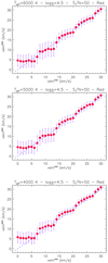 |
Figure A.1 Results of the Monte Carlo simulations on v sin i for red-arm LAMOST MRS. BT-Settl synthetic spectra with log g=4.5 and three different Teff values, as indicated in the title of each box, have been adopted. The S/N=50. The average v sin i values measured with our procedure (dots) are plotted against the “theoretical” v sin i to which the spectra have been broadened. The error bars represent the standard deviations of the 200 simulations at each v sin i. The 1:1 relation is plotted with a dashed blue line. |
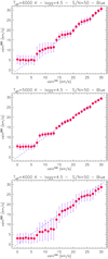 |
Figure A.2 Results of the Monte Carlo simulations on v sin i for blue-arm LAMOST MRS. The Teff, log g, and S/N are indicated in the top title of each box. The meaning of the symbols is the same as in Fig. A.1. |
Appendix B Stars with Discrepant Values of Stellar Parameters Compared to the Literature
We discuss in this section the stars whose Teff, log g, or [Fe/H] values appear as outliers in Figs. 7, 8, or 9 where we compare our APs determinations with those from the literature.
As regards the effective temperature, we note two stars, KIC 7612547 and KIC 8750025, with very discrepant values (∆Teff>1300 K) that are marked with their KIC identifiers in Fig. 7c. Furthermore, we measure a lower temperature for the very few objects with Teff> 7500 K in the APOGEE or LASP samples. This is obviously due to the template grid used by ROTFIT, which is optimized for FGKM stars and does not contain a sufficient number of hot stars.
As regards the gravity, we found three stars with discrepant log g values (∆log g>2.0 dex): KIC 8494839, KIC 8750025, and KIC 10526137. Those stars are marked in Figs. 8a, b, or c with their KIC identifiers.
Finally, as regards the metallicity, we notice a group of 27 stars (KIC 5949422, 5957774, 6127083, 6685477, 6849670, 6852771, 6862553, 6864450, 6938848, 6949847, 7039688, 7186646, 7287513, 7360068, 7532435, 7603295, 7691709, 7820467, 7880048, 7880839, 7949214, 8036035, 8169032, 8686000, 8950928, 9026866, and 9099050) for which the LASP pipeline produces very low values of [Fe/H] but which in the same time are found in this paper to be of solar metallicity. Those stars fall into a yellow rectangle in Fig. 9c and are discussed at the bottom of this section.
In Table B.1, we provide the APs derived from the LAMOST MRS spectroscopy in this paper for four stars indicated with their KIC numbers in Figs. 7 or Figs. 8. That table provides also the APs derived from the LAMOST MRS data by Zong et al. (2020) who used the LASP pipeline (two stars) or by Wang et al. (2020b) who used the Stellar Parameters and Chemical Abundances Network (SPCANet) neural network (two stars, we provide the mean values and their standard errors calculated from individual AP measurements), high-resolution spectroscopy by Jönsson et al. (2020) (two stars), Dartmouth stellar isochrones by Huber et al. (2014) (one star), the LAMOST low-resolution spectroscopy by Xiang et al. (2019) (two stars, for KIC 10526137 we provide the mean values and their standard errors calculated from two individual AP measurements), or the Bayesian stellar parameters derived from the Gaia DR2 parallaxes and optical photometry by Anders et al. (2019) (four stars). We note that not for all the literature values of APs listed in Table B.1 the 1σ uncertainties have been provided.
Since the APs of stars listed in Table B.1 show noticeable scatter, our general conclusion is that the APs derived by means of methods other than analysis of high-resolution spectroscopy should be taken with care, and the respective stars should be observed again, possibly with high-resolution spectroscopy.
 |
Figure B.1 Comparison of the [Fe/H] values derived by Zong et al. (2020) with the values reported in the literature. Different colors and symbols are used for different literature sources, as indicated in the text. The solid line is a linear fit to the data. The dotted line represents the one-to-one relationship. |
For KIC 7612547, which is marked in Fig. 7c, we found a very large discrepancy (≃ 1330 K) between our Teff value and the one derived with the LASP pipeline on the same spectra. However, the APs reported in the present work are in excellent agreement with those from the literature, as can be seen in Table B.1. Therefore, we conclude that our APs are fully reliable and the LASP values are affected by issues, as also apparent from their very large errors.
For KIC 8494839, which is marked in Figs. 8b and Figs. 8c, the log g value derived in this paper is significantly higher than the log g reported by Jönsson et al. (2020). We note, however, that this value was flagged by Jönsson et al. (2020) as possibly falling in an unreliable range of calibration determination. The log g value derived by Anders et al. (2019) falls in between the determinations reported in this paper and by Jönsson et al. (2020).
The APs of KIC 8750025, which is marked in Figs. 7c and 8c, are very different from the literature determination listed in Table B.1. Also, Gaia Collaboration et al. (2018), Kepler Mission Team (2009) or Pinsonneault et al. (2012) consistently point to a cool star of Teff between 4000 and 4500 K. In this paper, we analyzed ten LAMOST MRS measured in 2018 while Wang et al. (2020b) derived APs from two spectra measured in 2019 and one, in 2018. The APs derived by Wang et al. (2020b) from the spectrum acquired on May, 24, 2018, which was also analyzed in this paper, yielded Teff = 6135 ± 119 K, log g = 4.16±0.17 dex, and [Fe/H] = −0.09±0.12 dex (thus the large standard errors of the means listed in Table B.1), which agree with the APs we derived within the respective 1σ error bars. Since the reason for the discrepancy in the APs of KIC 8750025 derived from the LAMOST MRS measured in different seasons is not clear, we suggest using them with care.
According to our AP determinations, KIC 10526137, which is marked in Fig. 7a, is a late-type giant of metallicity slightly lower than solar. For that star, the APs reported in the literature show high dispersion (see Table B.1). In particular, the log g determinations range from 0.19 dex (Anders et al. 2019) to 5.30 dex (Xiang et al. 2019). Berger et al. (2018) who used the parallaxes from the Gaia DR 2 (Gaia Collaboration et al. 2018; Lindegren et al. 2018) and the DR25 Kepler Stellar Properties Catalog (Mathur et al. 2017) computed that radius of this star, R = 146.830 R⊙, and classified it as a red giant. We find the analyses based on the Gaia parallaxes carried out by Anders et al. (2019) and Berger et al. (2018) to be conclusive and the APs of KIC 10526137 derived in this paper to be fully reliable.
Figure B.1 shows the comparison of the [Fe/H] values derived from the MRS LAMOST spectra by Zong et al. (2020) and the literature values for the 27 stars that fall into the yellow rectangle in Fig. 9c. The [Fe/H] values derived in this paper are indicated with black open circles. Those derived from high-resolution APOGEE spectra by Jönsson et al. (2020) or Olney et al. (2020) are indicated with large purple dots. The [Fe/H] values derived from the MRS LAMOST spectra by Wang et al. (2020b) are indicated with green squares and those derived from the LRS LAMOST spectra by Xiang et al. (2019) are indicated with blue triangles. The linear fit to the data is plotted with a solid line. The linear regression gives a slope b = 0.96 and intercept a = 0.83.
Both this paper and Zong et al. (2020) find those 27 stars to be late-type giants cooler than ~4500 K. The discrepancies in [Fe/H] shown in Fig. B.1 highlight the necessity of using high-resolution spectroscopic analyses for deriving precise and accurate values of APs; they also show that in the discussed range of the APs neither LASP nor ROTFIT provide results that are fully reliable.
Appendix C Online Figures and Tables
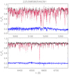 |
Figure C.1 Same as Fig. 3 but for a K0 III star. |
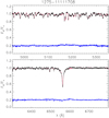 |
Figure C.2 Same as Fig. 3 but for a mid-F star rotating at about 110 km s−1. |
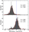 |
Figure C.3 Radial velocity difference of LK–MRS to Gaia (black histograms) for two plates calibrated with different lamps in the blue arm (top: 58267-HIPP95119KP01; bottom: 58263-HIP9511901). Red lines represent the best Gaussian fittings, whose centers and widths, μ and σ, are quoted in the legend. The vertical dotted blue line marks ∆RV=0. |
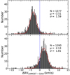 |
Figure C.4 Same as Fig. C.3 but for the red-arm RVs. |
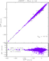 |
Figure C.5 Comparison between the RVs measured in this work on the blue-arm (Table C.3) and red-arm LAMOST MRS (Table C.2). The one-to-one relation is shown by the continuous line. The RV differences displayed in the lower box show an average value of −0.1 km s−1 (dashed line) and a standard deviation of 2.3 km s−1 (dotted lines). |
 |
Figure C.6 Observed continuum-normalized spectra of the stars with the strongest Hα flux (black dots), labeled according to Fig. 11. The best fitting template is overlaid with a red line. The differences observed – template are displayed in the bottom of the boxes, with blue lines for the stars with moderate emission. The Hα profile of star #5 is displayed in Fig. 10. |
Radial velocity corrections.
Stellar parameters and RVs derived with ROTFIT from the red−arm MRS LAMOST spectra.
Stellar parameters and RVs derived with ROTFIT from the blue-arm MRS LAMOST spectra.
Triple (SB3) and double-lined (SB2) systems.
Appendix D Spectral Energy Distribution
From optical BVg′r′i′ photometry taken from the AAVSO Photometric All Sky Survey (APASS) catalog (Henden et al. 2016) and near-infrared photometric data from 2MASS (Skrutskie et al. 2006), and mid-infrared WISE data (Cutri et al. 2021) we built the corresponding SED, which was fitted with BT-Settl synthetic spectra (Allard et al. 2012). For each target, we adopted its Gaia EDR3 parallax as well as the APs (Teff and log g) derived in the present work, leaving the stellar radius (R) and the interstellar extinction AV free to vary. The values of R and AV were then obtained by χ2 minimization of the flux differences between observed and synthetic SED. We fitted all the optical/near-infrared bands (BVg′ r′ i′ JHK), with the exception of stars with infrared excess for which J was the reddest band for the fit. Finally, the stellar luminosity was calculated as  . Some examples of this fitting are shown in Figs. D.1, D.2, and D.4. The errors on AV and R are found by the minimization procedure considering the 1σ confidence level of the χ2 map, but we have also taken the error on Teff into account.
 |
Figure D.1 Spectral energy distribution of the AGB star KIC 11657857. Optical fluxes from APASS (Henden et al. 2016) and near-infrared fluxes from the 2MASS catalog (Skrutskie et al. 2006) are displayed with colored dots. Mid- and far-infrared fluxes from WISE (Cutri et al. 2021), AKARI (Ishi-hara et al. 2010), and IRAS (Abrahamyan et al. 2015) are shown with diamonds, triangles, and squares, respectively. The BT-Settl spectrum (Allard et al. 2012) that provides the best fit to the star photosphere up to the J band is shown with a gray line. |
 |
Figure D.2 Spectral energy distribution of the Li-rich giant KIC 8363443 from the optical/near-infrared (colored dots) to the mid-infrared bands (diamonds). The BT-Settl spectrum (Allard et al. 2012) that provides the best fit to the star photosphere up to the K band is shown with a gray line. |
 |
Figure D.3 Spectral energy distribution of the possible Herbig star KIC 9720659 from the optical/near-infrared (colored dots) to the mid-infrared bands (diamonds). The BT-Settl spectrum (Allard et al. 2012) that provides the best fit to the star photosphere up to the J band is shown with a gray line. |
 |
Figure D.4 Spectral energy distribution of the active giant KIC 8749284. Mid-infrared fluxes are shown with different symbols (diamonds for WISE and a triangle for AKARI). The BT-Settl spectrum (Allard et al. 2012) that provides the best fit to the star photosphere up to the J band is shown with a gray line. |
References
- Abrahamyan, H.V., Mickaelian, A.M., & Knyazyan, A.V. 2015, Astron. Comput., 10, 99 [NASA ADS] [CrossRef] [Google Scholar]
- Abt, H.A., & Morrell, N.I. 1995, ApJS, 99, 135 [NASA ADS] [CrossRef] [Google Scholar]
- Abt, H.A., Levato, H., & Grosso, M. 2002, ApJ, 573, 359 [NASA ADS] [CrossRef] [Google Scholar]
- Aguilera-Gömez, C., Chanamé, J., Pinsonneault, M.H., & Carlberg, J.K. 2016, ApJ, 829, 127 [CrossRef] [Google Scholar]
- Alcalá, J.M., Biazzo, K., Covino, E., Frasca, A., & Bedin, L.R. 2011, A&A, 531, L12 [NASA ADS] [CrossRef] [EDP Sciences] [Google Scholar]
- Alcalâ, J.M., Gangi, M., Biazzo, K., et al. 2021, A&A, 652, A72 [NASA ADS] [CrossRef] [EDP Sciences] [Google Scholar]
- Allard, F. 2014, in Exploring the Formation and Evolution of Planetary Systems, eds. M. Booth, B.C. Matthews, & J.R. Graham, 299, 271 [NASA ADS] [Google Scholar]
- Allard, F., Homeier, D., & Freytag, B. 2012, Philos. Trans. R. Soc. Lond. A, 370, 2765 [Google Scholar]
- Allende Prieto, C., Majewski, S.R., Schiavon, R., et al. 2008, Astron. Nachr., 329, 1018 [NASA ADS] [CrossRef] [Google Scholar]
- Alonso-Santiago, J., Negueruela, I., Marco, A., et al. 2017, MNRAS, 469, 1330 [NASA ADS] [CrossRef] [Google Scholar]
- Alonso-Santiago, J., Negueruela, I., Marco, A., et al. 2019, A&A, 631, A124 [NASA ADS] [CrossRef] [EDP Sciences] [Google Scholar]
- Anders, F., Khalatyan, A., Chiappini, C., et al. 2019, A&A, 628, A94 [NASA ADS] [CrossRef] [EDP Sciences] [Google Scholar]
- Balona, L.A., Pigulski, A., De Cat, P., et al. 2011, MNRAS, 413, 2403 [NASA ADS] [CrossRef] [Google Scholar]
- Bastien, F.A., Stassun, K.G., Basri, G., & Pepper, J. 2016, ApJ, 818, 43 [NASA ADS] [CrossRef] [Google Scholar]
- Batalha, N.M., Rowe, J.F., Bryson, S.T., et al. 2013, ApJS, 204, 24 [NASA ADS] [CrossRef] [Google Scholar]
- Berger, T.A., Huber, D., Gaidos, E., & van Saders, J.L. 2018, ApJ, 866, 99 [NASA ADS] [CrossRef] [Google Scholar]
- Bevington, P.R., Robinson, D.K., Blair, J.M., Mallinckrodt, A.J., & McKay, S. 1993, Comput. Phys., 7, 415 [NASA ADS] [CrossRef] [Google Scholar]
- Bonsack, W.K. 1959, ApJ, 130, 843 [NASA ADS] [CrossRef] [Google Scholar]
- Bressan, A., Marigo, P., Girardi, L., et al. 2012, MNRAS, 427, 127 [NASA ADS] [CrossRef] [Google Scholar]
- Brewer, J.M., & Fischer, D.A. 2018, ApJS, 237, 38 [NASA ADS] [CrossRef] [Google Scholar]
- Brewer, J.M., Fischer, D.A., Valenti, J.A., & Piskunov, N. 2016, ApJS, 225, 32 [NASA ADS] [CrossRef] [Google Scholar]
- Brown, T.M., Latham, D.W., Everett, M.E., & Esquerdo, G.A. 2011, AJ, 142, 112 [NASA ADS] [CrossRef] [Google Scholar]
- Bruntt, H., Frandsen, S., & Thygesen, A.O. 2011, A&A, 528, A121 [NASA ADS] [CrossRef] [EDP Sciences] [Google Scholar]
- Bruntt, H., Basu, S., Smalley, B., et al. 2012, MNRAS, 423, 122 [Google Scholar]
- Buchhave, L.A., Latham, D.W., Johansen, A., et al. 2012, Nature, 486, 375 [NASA ADS] [CrossRef] [Google Scholar]
- Cameron, A.G.W., & Fowler, W.A. 1971, ApJ, 164, 111 [NASA ADS] [CrossRef] [Google Scholar]
- Cardini, D., & Cassatella, A. 2007, ApJ, 666, 393 [NASA ADS] [CrossRef] [Google Scholar]
- Carlberg, J.K., Cunha, K., Smith, V.V., & Majewski, S.R. 2012, ApJ, 757, 109 [NASA ADS] [CrossRef] [Google Scholar]
- Carney, B.W., Gray, D.F., Yong, D., et al. 2008, AJ, 135, 892 [NASA ADS] [CrossRef] [Google Scholar]
- Casagrande, L., Schönrich, R., Asplund, M., et al. 2011, A&A, 530, A138 [NASA ADS] [CrossRef] [EDP Sciences] [Google Scholar]
- Casagrande, L., Silva Aguirre, V., Stello, D., et al. 2014, ApJ, 787, 110 [CrossRef] [Google Scholar]
- Casagrande, L., Silva Aguirre, V., Schlesinger, K.J., et al. 2016, MNRAS, 455, 987 [NASA ADS] [CrossRef] [Google Scholar]
- Casey, A.R., Ruchti, G., Masseron, T., et al. 2016, MNRAS, 461, 3336 [NASA ADS] [CrossRef] [Google Scholar]
- Casey, A.R., Ho, A.Y.Q., Ness, M., et al. 2019, ApJ, 880, 125 [NASA ADS] [CrossRef] [Google Scholar]
- Catanzaro, G., Frasca, A., Molenda-Zakowicz, J., & Marilli, E. 2010, A&A, 517, A3 [NASA ADS] [CrossRef] [EDP Sciences] [Google Scholar]
- Catanzaro, G., Ripepi, V., Bernabei, S., et al. 2011, MNRAS, 411, 1167 [CrossRef] [Google Scholar]
- Charbonnel, C., & Balachandran, S.C. 2000, A&A, 359, 563 [Google Scholar]
- Christiansen, J.L., Jenkins, J.M., Caldwell, D.A., et al. 2012, PASP, 124, 1279 [NASA ADS] [CrossRef] [Google Scholar]
- Cui, X.-Q., Zhao, Y.-H., Chu, Y.-Q., et al. 2012, Res. Astron. Astrophys., 12, 1197 [Google Scholar]
- Cutri, R.M., Wright, E.L., Conrow, T., et al. 2021, VizieR Online Data Catalog: II/328 [Google Scholar]
- Davenport, J.R.A. 2016, ApJ, 829, 23 [NASA ADS] [CrossRef] [Google Scholar]
- De Cat, P., Fu, J.N., Ren, A.B., et al. 2015, ApJS, 220, 19 [NASA ADS] [CrossRef] [Google Scholar]
- de Medeiros, J.R., & Mayor, M. 1999, A&AS, 139, 433 [NASA ADS] [CrossRef] [EDP Sciences] [Google Scholar]
- Debosscher, J., Blomme, J., Aerts, C., & De Ridder, J. 2011, A&A, 529, A89 [NASA ADS] [CrossRef] [EDP Sciences] [Google Scholar]
- Deepak, & Reddy, B.E. 2019, MNRAS, 484, 2000 [NASA ADS] [Google Scholar]
- Delfosse, X., Forveille, T., Perrier, C., & Mayor, M. 1998, A&A, 331, 581 [NASA ADS] [Google Scholar]
- Deshpande, R., Blake, C.H., Bender, C.F., et al. 2013, AJ, 146, 156 [NASA ADS] [CrossRef] [Google Scholar]
- Dong, S., Zheng, Z., Zhu, Z., et al. 2014, ApJ, 789, L3 [NASA ADS] [CrossRef] [Google Scholar]
- Famaey, B., Jorissen, A., Luri, X., et al. 2005, A&A, 430, 165 [CrossRef] [EDP Sciences] [Google Scholar]
- Fehrenbach, C., Duflot, M., Mannone, C., Burnage, R., & Genty, V. 1997, A&AS, 124, 255 [NASA ADS] [CrossRef] [EDP Sciences] [Google Scholar]
- Fekel, F.C. 1997, PASP, 109, 514 [NASA ADS] [CrossRef] [Google Scholar]
- Frasca, A., & Catalano, S. 1994, A&A, 284, 883 [NASA ADS] [Google Scholar]
- Frasca, A., Alcalâ, J.M., Covino, E., et al. 2003, A&A, 405, 149 [NASA ADS] [CrossRef] [EDP Sciences] [Google Scholar]
- Frasca, A., Guillout, P., Marilli, E., et al. 2006, A&A, 454, 301 [NASA ADS] [CrossRef] [EDP Sciences] [Google Scholar]
- Frasca, A., Fröhlich, H.E., Bonanno, A., et al. 2011, A&A, 532, A81 [NASA ADS] [CrossRef] [EDP Sciences] [Google Scholar]
- Frasca, A., Biazzo, K., Lanzafame, A.C., et al. 2015, A&A, 575, A4 [NASA ADS] [CrossRef] [EDP Sciences] [Google Scholar]
- Frasca, A., Molenda-Zakowicz, J., De Cat, P., et al. 2016, A&A, 594, A39 [CrossRef] [EDP Sciences] [Google Scholar]
- Frasca, A., Biazzo, K., Alcalâ, J.M., et al. 2017, A&A, 602, A33 [NASA ADS] [CrossRef] [EDP Sciences] [Google Scholar]
- Frasca, A., Guillout, P., Klutsch, A., et al. 2018, A&A, 612, A96 [NASA ADS] [CrossRef] [EDP Sciences] [Google Scholar]
- Frinchaboy, P.M., & Majewski, S.R. 2008, AJ, 136, 118 [NASA ADS] [CrossRef] [Google Scholar]
- Fröhlich, H.E., Frasca, A., Catanzaro, G., et al. 2012, A&A, 543, A146 [CrossRef] [EDP Sciences] [Google Scholar]
- Fukugita, M., Ichikawa, T., Gunn, J.E., et al. 1996, AJ, 111, 1748 [NASA ADS] [CrossRef] [Google Scholar]
- Furlan, E., Ciardi, D.R., Cochran, W.D., et al. 2018, ApJ, 861, 149 [NASA ADS] [CrossRef] [Google Scholar]
- Gaia Collaboration (Brown, A.G.A., et al.) 2018, A&A, 616, A1 [NASA ADS] [CrossRef] [EDP Sciences] [Google Scholar]
- Gao, Q., Shi, J.-R., Yan, H.-L., et al. 2019, ApJS, 245, 33 [NASA ADS] [CrossRef] [Google Scholar]
- Gaulme, P., Jackiewicz, J., Spada, F., et al. 2020, A&A, 639, A63 [EDP Sciences] [Google Scholar]
- Gilmore, G., Randich, S., Asplund, M., et al. 2012, The Messenger, 147, 25 [NASA ADS] [Google Scholar]
- Gontcharov, G.A. 2006, Astron. Lett., 32, 759 [NASA ADS] [CrossRef] [Google Scholar]
- Goodarzi, H., Mehrabi, A., Khosroshahi, H.G., & He, H. 2019, ApJS, 244, 37 [NASA ADS] [CrossRef] [Google Scholar]
- Gorlova, N., Van Winckel, H., & Jorissen, A. 2012, Baltic Astron., 21, 165 [Google Scholar]
- Gratton, R., Sneden, C., & Carretta, E. 2004, ARA&A, 42, 385 [Google Scholar]
- Gray, D.F., & Toner, C.G. 1987, ApJ, 322, 360 [NASA ADS] [CrossRef] [Google Scholar]
- Gray, R.O., Corbally, C.J., De Cat, P., et al. 2016, AJ, 151, 13 [Google Scholar]
- Grenier, S., Baylac, M.O., Rolland, L., et al. 1999, A&AS, 137, 451 [NASA ADS] [CrossRef] [EDP Sciences] [Google Scholar]
- Grieves, N., Ge, J., Thomas, N., et al. 2018, MNRAS, 481, 3244 [Google Scholar]
- Guillout, P., Klutsch, A., Frasca, A., et al. 2009, A&A, 504, 829 [NASA ADS] [CrossRef] [EDP Sciences] [Google Scholar]
- Guo, X., Johnson, J.A., Mann, A.W., et al. 2017, ApJ, 838, 25 [NASA ADS] [CrossRef] [Google Scholar]
- Handler, G., & Shobbrook, R.R. 2002, MNRAS, 333, 251 [NASA ADS] [CrossRef] [Google Scholar]
- Hardegree-Ullman, K.K., Cushing, M.C., Muirhead, P.S., & Christiansen, J.L. 2019, AJ, 158, 75 [NASA ADS] [CrossRef] [Google Scholar]
- Hauck, B., & Mermilliod, M. 1998, A&AS, 129, 431 [NASA ADS] [CrossRef] [EDP Sciences] [Google Scholar]
- Hauschildt, P.H., Allard, F., & Baron, E. 1999, ApJ, 512, 377 [NASA ADS] [CrossRef] [Google Scholar]
- Helminiak, K.G., Konacki, M., Maehara, H., et al. 2019, MNRAS, 484, 451 [NASA ADS] [CrossRef] [Google Scholar]
- Henden, A.A., Templeton, M., Terrell, D., et al. 2016, VizieR Online Data Catalog: II/336 [Google Scholar]
- Hillenbrand, L.A., Hoffer, A.S., & Herczeg, G.J. 2013, AJ, 146, 85 [NASA ADS] [CrossRef] [Google Scholar]
- Ho, A.Y.Q., Ness, M.K., Hogg, D.W., et al. 2017, ApJ, 836, 5 [NASA ADS] [CrossRef] [Google Scholar]
- Holanda, N., Drake, N.A., & Pereira, C.B. 2020a, AJ, 159, 9 [Google Scholar]
- Holanda, N., Drake, N.A., & Pereira, C.B. 2020b, MNRAS, 498, 77 [NASA ADS] [CrossRef] [Google Scholar]
- Howarth, I.D., Siebert, K.W., Hussain, G.A.J., & Prinja, R.K. 1997, MNRAS, 284, 265 [NASA ADS] [CrossRef] [Google Scholar]
- Hubble, E. 1942, Science, 95, 212 [NASA ADS] [CrossRef] [Google Scholar]
- Huber, D., Chaplin, W.J., Christensen-Dalsgaard, J., et al. 2013, ApJ, 767, 127 [NASA ADS] [CrossRef] [Google Scholar]
- Huber, D., Silva Aguirre, V., Matthews, J.M., et al. 2014, ApJS, 211, 2 [NASA ADS] [CrossRef] [Google Scholar]
- Iben, I. Jr., 1967a, ApJ, 147, 650 [NASA ADS] [CrossRef] [Google Scholar]
- Iben, I. Jr., 1967b, ApJ, 147, 624 [NASA ADS] [CrossRef] [Google Scholar]
- Ishihara, D., Onaka, T., Kataza, H., et al. 2010, A&A, 514, A1 [NASA ADS] [CrossRef] [EDP Sciences] [Google Scholar]
- Jackson, R.J., Jeffries, R.D., Lewis, J., et al. 2015, A&A, 580, A75 [NASA ADS] [CrossRef] [EDP Sciences] [Google Scholar]
- Jönsson, H., Holtzman, J.A., Allende Prieto, C., et al. 2020, AJ, 160, 120 [CrossRef] [Google Scholar]
- Kepler Mission Team. 2009, VizieR Online Data Catalog: V/133 [Google Scholar]
- Kharchenko, N.V., Scholz, R.D., Piskunov, A.E., Röser, S., & Schilbach, E. 2007, Astron. Nachr., 328, 889 [NASA ADS] [CrossRef] [Google Scholar]
- Kirby, E.N., Guhathakurta, P., Zhang, A.J., et al. 2016, ApJ, 819, 135 [NASA ADS] [CrossRef] [Google Scholar]
- Koenig, X.P., Leisawitz, D.T., Benford, D.J., et al. 2012, ApJ, 744, 130 [NASA ADS] [CrossRef] [Google Scholar]
- Küker, M., Rüdiger, G., Oláh, K., & Strassmeier, K.G. 2019, A&A, 622, A40 [NASA ADS] [CrossRef] [EDP Sciences] [Google Scholar]
- Kumar, Y.B., & Reddy, B.E. 2020, J. Astrophys. Astron., 41, 49 [NASA ADS] [CrossRef] [Google Scholar]
- Lambert, D.L., & Ries, L.M. 1981, ApJ, 248, 228 [NASA ADS] [CrossRef] [Google Scholar]
- Lee, J.W., & Park, J.-H. 2018, MNRAS, 480, 4693 [NASA ADS] [CrossRef] [Google Scholar]
- Lehmann, H., Tkachenko, A., Semaan, T., et al. 2011, A&A, 526, A124 [CrossRef] [EDP Sciences] [Google Scholar]
- Lind, K., Asplund, M., & Barklem, P.S. 2009, A&A, 503, 541 [NASA ADS] [CrossRef] [EDP Sciences] [Google Scholar]
- Lindegren, L., Hernandez, J., Bombrun, A., et al. 2018, A&A, 616, A2 [NASA ADS] [CrossRef] [EDP Sciences] [Google Scholar]
- Linsky, J.L., Hunten, D.M., Sowell, R., Glackin, D.L., & Kelch, W.L. 1979, ApJS, 41, 481 [NASA ADS] [CrossRef] [Google Scholar]
- Liu, N., Fu, J.-N., Zong, W., et al. 2019, Res. Astron. Astrophys., 19, 075 [CrossRef] [Google Scholar]
- Lomaeva, M., Jönsson, H., Ryde, N., Schultheis, M., & Thorsbro, B. 2019, A&A, 625, A141 [NASA ADS] [CrossRef] [EDP Sciences] [Google Scholar]
- Lucey, M., Ting, Y.-S., Ramachandra, N.S., & Hawkins, K. 2020, MNRAS, 495, 3087 [NASA ADS] [CrossRef] [Google Scholar]
- Luck, R.E. 1982, PASP, 94, 811 [NASA ADS] [CrossRef] [Google Scholar]
- Luo, A.L., Zhang, H.-T., Zhao, Y.-H., et al. 2012, Res. Astron. Astrophys., 12, 1243 [CrossRef] [Google Scholar]
- Luo, A.L., Zhao, Y.-H., Zhao, G., et al. 2015, Res. Astron. Astrophys., 15, 1095 [Google Scholar]
- Luo, A.L., Zhao, Y.H., Zhao, G., et al. 2016, VizieR Online Data Catalog: V/149 [Google Scholar]
- Luo, A.L., Zhao, Y.H., Zhao, G., et al. 2018, VizieR Online Data Catalog: V/153 [Google Scholar]
- Magrini, L., Smiljanic, R., Franciosini, E., et al. 2021, A&A, 655, A23 [NASA ADS] [CrossRef] [EDP Sciences] [Google Scholar]
- Mann, A.W., Gaidos, E., Lépine, S., & Hilton, E.J. 2012, ApJ, 753, 90 [NASA ADS] [CrossRef] [Google Scholar]
- Marcy, G.W., Isaacson, H., Howard, A.W., et al. 2014, ApJS, 210, 20 [NASA ADS] [CrossRef] [Google Scholar]
- Martell, S.L., Simpson, J.D., Balasubramaniam, A.G., et al. 2021, MNRAS, 505, 5340 [NASA ADS] [Google Scholar]
- Martinez-Arnâiz, R., Löpez-Santiago, J., Crespo-Chacön, I., & Montes, D. 2011, MNRAS, 414, 2629 [CrossRef] [Google Scholar]
- Mathur, S., Huber, D., Batalha, N.M., et al. 2017, ApJS, 229, 30 [NASA ADS] [CrossRef] [Google Scholar]
- Matson, R.A., Gies, D.R., Guo, Z., & Williams, S.J. 2017, AJ, 154, 216 [NASA ADS] [CrossRef] [Google Scholar]
- Mazeh, T., Perets, H.B., McQuillan, A., & Goldstein, E.S. 2015, ApJ, 801, 3 [Google Scholar]
- McNamara, B.J., Jackiewicz, J., & McKeever, J. 2012, AJ, 143, 101 [NASA ADS] [CrossRef] [Google Scholar]
- McQuillan, A., Mazeh, T., & Aigrain, S. 2013, ApJ, 775, L11 [Google Scholar]
- McQuillan, A., Mazeh, T., & Aigrain, S. 2014, ApJS, 211, 24 [Google Scholar]
- Mermilliod, J.C., Mayor, M., & Udry, S. 2008, A&A, 485, 303 [NASA ADS] [CrossRef] [EDP Sciences] [Google Scholar]
- Mészâros, S., Holtzman, J., Garcia Pérez, A.E., et al. 2013, AJ, 146, 133 [CrossRef] [Google Scholar]
- Molenda-Zakowicz, J., Frasca, A., Latham, D.W., & Jerzykiewicz, M. 2007, Acta Astron., 57, 301 [NASA ADS] [Google Scholar]
- Molenda-Zakowicz, J., Frasca, A., & Latham, D.W. 2008, Acta Astron., 58, 419 [NASA ADS] [Google Scholar]
- Molenda-Zakowicz, J., Latham, D.W., Catanzaro, G., Frasca, A., & Quinn, S.N. 2011, MNRAS, 412, 1210 [NASA ADS] [Google Scholar]
- Molenda-Zakowicz, J., Sousa, S.G., Frasca, A., et al. 2013, MNRAS, 434, 1422 [NASA ADS] [CrossRef] [Google Scholar]
- Molenda-Zakowicz, J., Brogaard, K., Niemczura, E., et al. 2014, MNRAS, 445, 2446 [CrossRef] [Google Scholar]
- Monaco, L., Boffin, H.M.J., Bonifacio, P., et al. 2014, A&A, 564, L6 [NASA ADS] [CrossRef] [EDP Sciences] [Google Scholar]
- Montes, D., Fernandez-Figueroa, M.J., de Castro, E., & Cornide, M. 1995, A&A, 294, 165 [NASA ADS] [Google Scholar]
- Montes, D., Löpez-Santiago, J., Fernândez-Figueroa, M.J., & Gâlvez, M.C. 2001, A&A, 379, 976 [CrossRef] [EDP Sciences] [Google Scholar]
- Moultaka, J., Ilovaisky, S.A., Prugniel, P., & Soubiran, C. 2004, PASP, 116, 693 [NASA ADS] [CrossRef] [Google Scholar]
- Neuhaeuser, R., Torres, G., Sterzik, M.F., & Randich, S. 1997, A&A, 325, 647 [NASA ADS] [Google Scholar]
- Nidever, D.L., Marcy, G.W., Butler, R.P., Fischer, D.A., & Vogt, S.S. 2002, ApJS, 141, 503 [NASA ADS] [CrossRef] [Google Scholar]
- Nielsen, M.B., Schunker, H., Gizon, L., & Ball, W.H. 2015, A&A, 582, A10 [NASA ADS] [CrossRef] [EDP Sciences] [Google Scholar]
- Niemczura, E., Murphy, S.J., Smalley, B., et al. 2015, MNRAS, 450, 2764 [NASA ADS] [CrossRef] [Google Scholar]
- Niemczura, E., Polmska, M., Murphy, S.J., et al. 2017, MNRAS, 470, 2870 [NASA ADS] [CrossRef] [Google Scholar]
- Nordström, B., Mayor, M., Andersen, J., et al. 2004, A&A, 418, 989 [Google Scholar]
- Notsu, Y., Honda, S., Maehara, H., et al. 2015, PASJ, 67, 32 [NASA ADS] [CrossRef] [Google Scholar]
- O'Dell, C.R., Peimbert, M., & Peimbert, A. 2003, AJ, 125, 2590 [CrossRef] [Google Scholar]
- Oláh, K., Kovâri, Z., Günther, M.N., et al. 2021, A&A, 647, A62 [NASA ADS] [CrossRef] [EDP Sciences] [Google Scholar]
- Olney, R., Kounkel, M., Schillinger, C., et al. 2020, AJ, 159, 182 [NASA ADS] [CrossRef] [Google Scholar]
- Pakhomov, Y.V., Antipova, L.I., Boyarchuk, A.A., Zhao, G., & Liang, Y. 2009, Astron. Rep., 53, 685 [NASA ADS] [CrossRef] [Google Scholar]
- Pan, Y., Fu, J.-N., Zong, W., et al. 2020, ApJ, 905, 67 [NASA ADS] [CrossRef] [Google Scholar]
- Pérez, A.E.G., Prieto, C.A., Holtzman, J.A., et al. 2016, Astron. J., 151, 144 [CrossRef] [Google Scholar]
- Petigura, E.A., Marcy, G.W., & Howard, A.W. 2013, ApJ, 770, 69 [NASA ADS] [CrossRef] [Google Scholar]
- Petigura, E.A., Howard, A.W., Marcy, G.W., et al. 2017, AJ, 154, 107 [NASA ADS] [CrossRef] [Google Scholar]
- Pigulski, A., Pojmanski, G., Pilecki, B., & Szczygiel, D.M. 2009, Acta Astron., 59, 33 [NASA ADS] [Google Scholar]
- Pinsonneault, M.H., An, D., Molenda-Zakowicz, J., et al. 2012, ApJS, 199, 30 [NASA ADS] [CrossRef] [Google Scholar]
- Pinsonneault, M.H., Elsworth, Y., Epstein, C., et al. 2014, ApJS, 215, 19 [NASA ADS] [CrossRef] [Google Scholar]
- Pizzolato, N., Maggio, A., Micela, G., Sciortino, S., & Ventura, P. 2003, A&A, 397, 147 [NASA ADS] [CrossRef] [EDP Sciences] [Google Scholar]
- Pojmanski, G. 1997, Acta Astron., 47, 467 [Google Scholar]
- Press, W.H., Teukolsky, S.A., Vetterling, W.T., & Flannery, B.P. 1992, Numerical recipes in FORTRAN. The art of scientific computing [Google Scholar]
- Privitera, G., Meynet, G., Eggenberger, P., et al. 2016, A&A, 593, A128 [NASA ADS] [CrossRef] [EDP Sciences] [Google Scholar]
- Queloz, D., Allain, S., Mermilliod, J.C., Bouvier, J., & Mayor, M. 1998, A&A, 335, 183 [Google Scholar]
- Ramsay, G., Doyle, J.G., & Doyle, L. 2020, MNRAS, 497, 2320 [NASA ADS] [CrossRef] [Google Scholar]
- Reiners, A., Schüssler, M., & Passegger, V.M. 2014, ApJ, 794, 144 [NASA ADS] [CrossRef] [Google Scholar]
- Reinhold, T., Reiners, A., & Basri, G. 2013, A&A, 560, A4 [NASA ADS] [CrossRef] [EDP Sciences] [Google Scholar]
- Ren, A., Fu, J., De Cat, P., et al. 2016, ApJS, 225, 28 [NASA ADS] [CrossRef] [Google Scholar]
- Roberts, D.H., Lehar, J., & Dreher, J.W. 1987, AJ, 93, 968 [NASA ADS] [CrossRef] [Google Scholar]
- Rodriguez, E. & Breger, M. 2001, A&A, 366, 178 [NASA ADS] [CrossRef] [EDP Sciences] [Google Scholar]
- Royer, F., Grenier, S., Baylac, M.O., Gömez, A.E., & Zorec, J. 2002, A&A, 393, 897 [NASA ADS] [CrossRef] [EDP Sciences] [Google Scholar]
- Saar, S.H., & Osten, R.A. 1997, MNRAS, 284, 803 [NASA ADS] [CrossRef] [Google Scholar]
- Sarmento, P., Delgado Mena, E., Rojas-Ayala, B., & Blanco-Cuaresma, S. 2020, A&A, 636, A85 [NASA ADS] [CrossRef] [EDP Sciences] [Google Scholar]
- Scargle, J.D. 1982, ApJ, 263, 835 [NASA ADS] [CrossRef] [Google Scholar]
- Schmidt, E.G., Langan, S., Rogalla, D., & Thacker-Lynn, L. 2007, AJ, 133, 665 [NASA ADS] [CrossRef] [Google Scholar]
- Schmidt, E.G., Rogalla, D., & Thacker-Lynn, L. 2011, AJ, 141, 53 [NASA ADS] [CrossRef] [Google Scholar]
- Sestito, P., & Randich, S. 2005, A&A, 442, 615 [NASA ADS] [CrossRef] [EDP Sciences] [Google Scholar]
- Siess, L., & Livio, M. 1999, MNRAS, 308, 1133 [Google Scholar]
- Singh, R., Reddy, B.E., Bharat Kumar, Y., & Antia, H.M. 2019, ApJ, 878, L21 [NASA ADS] [CrossRef] [Google Scholar]
- Skrutskie, M.F., Cutri, R.M., Stiening, R., et al. 2006, AJ, 131, 1163 [NASA ADS] [CrossRef] [Google Scholar]
- Smiljanic, R., Franciosini, E., Bragaglia, A., et al. 2018, A&A, 617, A4 [NASA ADS] [CrossRef] [EDP Sciences] [Google Scholar]
- Soderblom, D.R., Oey, M.S., Johnson, D.R.H., & Stone, R.P.S. 1990, AJ, 99, 595 [NASA ADS] [CrossRef] [Google Scholar]
- Soderblom, D.R., Jones, B.F., Balachandran, S., et al. 1993a, AJ, 106, 1059 [NASA ADS] [CrossRef] [Google Scholar]
- Soderblom, D.R., Pilachowski, C.A., Fedele, S.B., & Jones, B.F. 1993b, AJ, 105, 2299 [NASA ADS] [CrossRef] [Google Scholar]
- Stauffer, J.R., Hartmann, L.W., Prosser, C.F., et al. 1997, ApJ, 479, 776 [NASA ADS] [CrossRef] [Google Scholar]
- Steinmetz, M., Zwitter, T., Siebert, A., et al. 2006, AJ, 132, 1645 [Google Scholar]
- Thygesen, A.O., Frandsen, S., Bruntt, H., et al. 2012, A&A, 543, A160 [NASA ADS] [CrossRef] [EDP Sciences] [Google Scholar]
- Tian, H.-J., El-Badry, K., Rix, H.-W., & Gould, A. 2020, ApJS, 246, 4 [Google Scholar]
- Tkachenko, A., Lehmann, H., Smalley, B., Debosscher, J., & Aerts, C. 2012, MNRAS, 422, 2960 [Google Scholar]
- Tkachenko, A., Aerts, C., Yakushechkin, A., et al. 2013, A&A, 556, A52 [NASA ADS] [CrossRef] [EDP Sciences] [Google Scholar]
- Tonry, J., & Davis, M. 1979, AJ, 84, 1511 [Google Scholar]
- Torres, G., Fischer, D.A., Sozzetti, A., et al. 2012, ApJ, 757, 161 [NASA ADS] [CrossRef] [Google Scholar]
- Tucker, D.L., Kent, S., Richmond, M.W., et al. 2006, Astron. Nachr., 327, 821 [NASA ADS] [CrossRef] [Google Scholar]
- Udalski, A., Szymanski, M., Kaluzny, J., Kubiak, M., & Mateo, M. 1992, Acta Astron., 42, 253 [NASA ADS] [Google Scholar]
- Uytterhoeven, K., Briquet, M., Bruntt, H., et al. 2010, Astron. Nachr., 331, 993 [NASA ADS] [CrossRef] [Google Scholar]
- Uytterhoeven, K., Moya, A., Grigahcène, A., et al. 2011, A&A, 534, A125 [CrossRef] [EDP Sciences] [Google Scholar]
- Valdes, F., Gupta, R., Rose, J.A., Singh, H.P., & Bell, D.J. 2004, ApJS, 152, 251 [NASA ADS] [CrossRef] [Google Scholar]
- Walkowicz, L.M., Basri, G., Batalha, N., et al. 2011, AJ, 141, 50 [NASA ADS] [CrossRef] [Google Scholar]
- Wallerstein, G., & Sneden, C. 1982, ApJ, 255, 577 [NASA ADS] [CrossRef] [Google Scholar]
- Wang, S.-G., Su, D.-Q., Chu, Y.-Q., Cui, X., & Wang, Y.-N. 1996, Appl. Opt., 35, 5155 [NASA ADS] [CrossRef] [Google Scholar]
- Wang, J., Fischer, D.A., Barclay, T., et al. 2013, ApJ, 776, 10 [NASA ADS] [CrossRef] [Google Scholar]
- Wang, R., Luo, A.L., Chen, J.J., et al. 2019, ApJS, 244, 27 [NASA ADS] [CrossRef] [Google Scholar]
- Wang, J., Fu, J.-N., Zong, W., et al. 2020a, ApJS, 251, 27 [NASA ADS] [CrossRef] [Google Scholar]
- Wang, R., Luo, A.L., Chen, J.-J., et al. 2020b, ApJ, 891, 23 [NASA ADS] [CrossRef] [Google Scholar]
- Wang, J., Fu, J., Niu, H., et al. 2021, MNRAS, 504, 4302 [NASA ADS] [CrossRef] [Google Scholar]
- White, R.J., Gabor, J.M., & Hillenbrand, L.A. 2007, AJ, 133, 2524 [NASA ADS] [CrossRef] [Google Scholar]
- Wilson, R.E. 1953, Carnegie Institute Washington D.C. Publication, 0 [Google Scholar]
- Woosley, S.E., & Weaver, T.A. 1995, ApJS, 101, 181 [NASA ADS] [CrossRef] [Google Scholar]
- Wu, Y., Singh, H.P., Prugniel, P., Gupta, R., & Koleva, M. 2011, A&A, 525, A71 [NASA ADS] [CrossRef] [EDP Sciences] [Google Scholar]
- Wu, Y., Du, B., Luo, A., Zhao, Y., & Yuan, H. 2014, in Statistical Challenges in 21st Century Cosmology, eds. A. Heavens, J.-L. Starck, & A. Krone-Martins, Vol. 306, 340 [NASA ADS] [Google Scholar]
- Xiang, M., Ting, Y.-S., Rix, H.-W., et al. 2019, ApJS, 245, 34 [Google Scholar]
- Xing, X., Zhai, C., Du, H., et al. 1998, SPIE Conf. Ser., 3352, 839 [NASA ADS] [Google Scholar]
- Yang, H., & Liu, J. 2019, ApJS, 241, 29 [NASA ADS] [CrossRef] [Google Scholar]
- Yang, H., Liu, J., Gao, Q., et al. 2017, ApJ, 849, 36 [NASA ADS] [CrossRef] [Google Scholar]
- Yanny, B., Rockosi, C., Newberg, H.J., et al. 2009, AJ, 137, 4377 [CrossRef] [Google Scholar]
- York, D.G., Adelman, J., Anderson, John E., J., et al. 2000, AJ, 120, 1579 [NASA ADS] [CrossRef] [Google Scholar]
- Zhang, X., Jeffery, C.S., Li, Y., & Bi, S. 2020, ApJ, 889, 33 [NASA ADS] [CrossRef] [Google Scholar]
- Zhang, B., Li, J., Yang, F., et al. 2021, ApJS, 256, 14 [NASA ADS] [CrossRef] [Google Scholar]
- Zhao, G., Chen, Y.-Q., Shi, J.-R., et al. 2006, Chinese J. Astron. Astrophys., 6, 265 [NASA ADS] [CrossRef] [Google Scholar]
- Zhao, G., Zhao, Y.-H., Chu, Y.-Q., Jing, Y.-P., & Deng, L.-C. 2012, Res. Astron. Astrophys., 12, 723 [NASA ADS] [CrossRef] [Google Scholar]
- Zheng, Z.-P., Qiu, B., Luo, A.L., & Li, Y.-B. 2020, PASP, 132, 024504 [NASA ADS] [CrossRef] [Google Scholar]
- Zong, W., Fu, J.-N., De Cat, P., et al. 2018, ApJS, 238, 30 [NASA ADS] [CrossRef] [Google Scholar]
- Zong, W., Fu, J.-N., De Cat, P., et al. 2020, ApJS, 251, 15 [NASA ADS] [CrossRef] [Google Scholar]
Although these stars were selected as giants, they could actually be at the end of the subgiant phase according to the HR diagram in Fig. 15. Regardless of this group, the fraction of Li-rich giants is still very high, 5.5%. Even when considering the stars over the strip or those that have already passed it but whose positions, within the errors, might be indicating that they are still over or slightly before the strip (≈ 45 stars), the fraction of Li-rich giants would be around 4.2%, still much higher than the 1.3% found by other authors.
In line with other works (e.g., Carlberg et al. 2012; Martell et al. 2021), we considered 10 km s−1 an adequate value to separate fast from slow rotators since the typical v sin i among giants is around 3−5 km s−1 and the macroturbulence velocity ≈7 km s−1 (Carney et al. 2008).
All Tables
Overview of the LK–MRS plates observed in the period September 2017–June 2018 that have objects in common with the Kepler field.
Percentages of fast rotators (v sin i ≥ 10 km s−1) and stars with a solar metallicity (i.e., −0.2 ≤ [Fe/H] ≤ +0.2) among the Li-normal and Li-rich giants.
Stellar parameters and RVs derived with ROTFIT from the red−arm MRS LAMOST spectra.
Stellar parameters and RVs derived with ROTFIT from the blue-arm MRS LAMOST spectra.
All Figures
 |
Fig. 1 Selection of the DR6 LK-MRS project data in the Kepler field. The stars observed on plates that have overlap with the Kepler CCDs are shown as dots (blue for stars on a Kepler CCD, dark blue for observations in 2017, and light blue for observations in 2018). |
| In the text | |
 |
Fig. 2 Errors of v sin i, RV, Teff, log g, and [Fe/H] (from top to bottom) as a function of the S/N for the blue-arm and red-arm spectra. The full cyan and yellow lines in each box are the median of the blue-arm and red-arm errors, respectively. The blue and red histograms in the right panels display the distributions of these errors for the blue-arm and redarm spectra, respectively. |
| In the text | |
 |
Fig. 3 Example of the continuum-normalized LAMOST spectrum of a slowly rotating mid-F star (dots) in the blue arm (upper panel) and in the red arm (lower panel). The best template found by ROTFIT is overplotted with a thin red line. The difference between the two spectra is shown in the bottom of each panel with a blue line shifted upward by 0.2. |
| In the text | |
 |
Fig. 4 Comparison of the parameters obtained from both arms. Typical errors are displayed in the bottom-right corner of each panel. In the panel corresponding to the v sin i, the dashed lines show the upper limit at 8 km s−1. |
| In the text | |
 |
Fig. 5 Differences obtained from both arms (blue and red) for each parameter. In the panel corresponding to the v sin i, the dashed line shows the upper limit at 8 km s−1. |
| In the text | |
 |
Fig. 6 Comparison with the APOGEE RVs. Upper-left panel: comparison between the RV measured on the blue-arm LAMOST MRS (Table C.3) and APOGEE values (Jönsson et al. 2020). Filled symbols represent the stars with multiple spectra. The one-to-one relation is shown by the continuous line. The RV differences between LAMOST and APOGEE, ∆RV, are displayed in the lower box and show an average value of 0.0 km s−1 (dashed line) and a standard deviation of 6.1 km s−1 (dotted lines). Upper-right panel: same as the upper-left panel but for the red-arm RVs listed in Table C.2. The purple squares in both panels enclose the more discrepant points (more than four times the rms). The distributions of the RV differences are shown by the histograms in the lower panels. The Gaussian fits are overplotted with black lines, and the center (μ) and dispersion (σ) of the Gaussians are also marked in these boxes. |
| In the text | |
 |
Fig. 7 Comparison of Teff values. (a) Comparison between the values of effective temperature in our database of LAMOST spectra and in the literature. Filled symbols represent dwarfs (log gROTFIT ≥ 3.5), open symbols represent giants (log gROTFIT < 3.5). Different colors have been used for different literature sources, as indicated in the main text. The comparison with the APOGEE and LASP Teff is shown in the middle (b) and bottom (c) panels, respectively. The dotted lines in the top box of each panel represent one-to-one relationships. The solid lines are linear fits to the data. The differences between ROTFIT and literature parameters are shown in the lower parts of each panel along with their average values and standard deviations. Stars indicated with arrows are discussed in the text. |
| In the text | |
 |
Fig. 8 Comparison of log g values derived in the present work with those from the literature (a), APOGEE (b), and LASP (c). The meaning of lines and symbols is as in Fig. 7. |
| In the text | |
 |
Fig. 9 Comparison of [Fe/H] values derived in the present work with those from the literature (a), APOGEE (b), and LASP (c). The meaning of lines and symbols is as in Fig. 7. The sources enclosed in the yellow rectangle in box (c) are discussed in Appendix B. |
| In the text | |
 |
Fig. 10 Example of the subtraction of the best non-active, lithium-poor template (red line) from the spectrum of KIC 8095028 (black dots), which reveals the chromospheric emission in the Hα core (blue line in the top panel) and emphasizes the Li I λ6708 Å absorption line, with the nearby blended lines removed (bottom panel). |
| In the text | |
 |
Fig. 11 Activity indicators. Left panel: Hα flux versus Teff (open circles for giants, purple dots for MS stars). Right panel: |
| In the text | |
 |
Fig. 12 Equivalent width of the Li I λ6707.8 line (WLi) plotted as a function of Teff (open circles for giants, purple dots for MS stars). The lines show the upper boundaries for Hyades (dash-dotted blue), Pleiades (solid red for both the lower and upper boundary), and IC 2602 (dashed orange) clusters. Most of the stars with a strong lithium absorption are lithium-rich giants. |
| In the text | |
 |
Fig. 13 Lithium abundance as a function of Teff. The upper envelopes of A(Li) for IC 2602, Pleiades, NGC 6475 (age ≈ 300 Myr), and Hyades clusters adapted from Sestito & Randich (2005) are overplotted. The meaning of the symbols is the same as in Fig. 12. |
| In the text | |
 |
Fig. 14 Kiel (Teff−log g) diagram for the final sample of the stars observed in this work. The left panel shows the stellar density and the right one highlights the position of the Li-rich (1.5 ≤ A(Li) < 2.7) and super Li-rich giants (A(Li) ≥ 2.7). The dashed lines delimit the area populated by giants according to our selection criteria, as explained in the text. |
| In the text | |
 |
Fig. 15 Hertzsprung-Russell diagram for all the Li-rich giants. The symbols are color coded by the lithium abundance A(Li). The PARSEC post-MS evolutionary tracks (Bressan et al. 2012) for a metallicity Z = 0.017 are plotted with black lines. The green and orange strips mark the base of the RGB and the RGB bump, respectively. |
| In the text | |
 |
Fig. 16 Abundance of Li as a function of the ν sin i among our Li-rich giant sample. The vertical line shows the limit between slow and fast rotators, while the horizontal one represents the boundary between Li-rich and super Li-rich giants. |
| In the text | |
 |
Fig. 17 Spectrum of KIC 11657857 (black line and dots), the star with the highest abundance of Li in our sample, versus that of a Li-normal giant with similar stellar parameters (red line) around the Li line at 6708 Å, whose center is marked with a vertical dashed line. |
| In the text | |
 |
Fig. 18 Cross-correlation function (black line) for a double-lined spectroscopic binary (SB2) in the blue arm (upper panel) and in the red arm (lower panel). The two-Gaussian fit of CCF is displayed with a green line, and the centers of the primary (more luminous) and secondary components are indicated with vertical dotted blue and red lines, respectively. |
| In the text | |
 |
Fig. 19 Radial velocity curve of KIC 7821010. The RV data from Helminiak et al. (2019) are shown with blue and red squares and the orbital solution with dotted blue and red lines for the primary and secondary component, respectively. The LAMOST MRS RVs derived in this work are overplotted with filled black circles for the primary and open circles for the secondary component, respectively. The green x symbols display the RV values measured by us near the conjunctions, where a single peak is visible in the CCF. |
| In the text | |
 |
Fig. 20 Radial velocity curve of KIC 6206751. The RV data from Matson et al. (2017) are displayed with blue and red squares and the orbital solution with dotted blue and red lines for the primary and secondary component, respectively. The LAMOST MRS RVs derived in this work are overplotted with filled black circles for the primary and open black circles for the secondary component. The green x symbols display the RV values measured by us near the conjunctions, where a single peak is visible in the CCF. |
| In the text | |
 |
Fig. 21 Radial velocity curve of KIC 10274200. The LAMOST MRS RVs derived in this work are plotted with filled circles for the primary and open circles for the secondary component. The green x symbols display the RV values measured near the conjunctions, where a single peak is visible in the CCF. The orbital solution is displayed with a dotted blue and red line for the primary and secondary component, respectively. |
| In the text | |
 |
Figure A.1 Results of the Monte Carlo simulations on v sin i for red-arm LAMOST MRS. BT-Settl synthetic spectra with log g=4.5 and three different Teff values, as indicated in the title of each box, have been adopted. The S/N=50. The average v sin i values measured with our procedure (dots) are plotted against the “theoretical” v sin i to which the spectra have been broadened. The error bars represent the standard deviations of the 200 simulations at each v sin i. The 1:1 relation is plotted with a dashed blue line. |
| In the text | |
 |
Figure A.2 Results of the Monte Carlo simulations on v sin i for blue-arm LAMOST MRS. The Teff, log g, and S/N are indicated in the top title of each box. The meaning of the symbols is the same as in Fig. A.1. |
| In the text | |
 |
Figure B.1 Comparison of the [Fe/H] values derived by Zong et al. (2020) with the values reported in the literature. Different colors and symbols are used for different literature sources, as indicated in the text. The solid line is a linear fit to the data. The dotted line represents the one-to-one relationship. |
| In the text | |
 |
Figure C.1 Same as Fig. 3 but for a K0 III star. |
| In the text | |
 |
Figure C.2 Same as Fig. 3 but for a mid-F star rotating at about 110 km s−1. |
| In the text | |
 |
Figure C.3 Radial velocity difference of LK–MRS to Gaia (black histograms) for two plates calibrated with different lamps in the blue arm (top: 58267-HIPP95119KP01; bottom: 58263-HIP9511901). Red lines represent the best Gaussian fittings, whose centers and widths, μ and σ, are quoted in the legend. The vertical dotted blue line marks ∆RV=0. |
| In the text | |
 |
Figure C.4 Same as Fig. C.3 but for the red-arm RVs. |
| In the text | |
 |
Figure C.5 Comparison between the RVs measured in this work on the blue-arm (Table C.3) and red-arm LAMOST MRS (Table C.2). The one-to-one relation is shown by the continuous line. The RV differences displayed in the lower box show an average value of −0.1 km s−1 (dashed line) and a standard deviation of 2.3 km s−1 (dotted lines). |
| In the text | |
 |
Figure C.6 Observed continuum-normalized spectra of the stars with the strongest Hα flux (black dots), labeled according to Fig. 11. The best fitting template is overlaid with a red line. The differences observed – template are displayed in the bottom of the boxes, with blue lines for the stars with moderate emission. The Hα profile of star #5 is displayed in Fig. 10. |
| In the text | |
 |
Figure D.1 Spectral energy distribution of the AGB star KIC 11657857. Optical fluxes from APASS (Henden et al. 2016) and near-infrared fluxes from the 2MASS catalog (Skrutskie et al. 2006) are displayed with colored dots. Mid- and far-infrared fluxes from WISE (Cutri et al. 2021), AKARI (Ishi-hara et al. 2010), and IRAS (Abrahamyan et al. 2015) are shown with diamonds, triangles, and squares, respectively. The BT-Settl spectrum (Allard et al. 2012) that provides the best fit to the star photosphere up to the J band is shown with a gray line. |
| In the text | |
 |
Figure D.2 Spectral energy distribution of the Li-rich giant KIC 8363443 from the optical/near-infrared (colored dots) to the mid-infrared bands (diamonds). The BT-Settl spectrum (Allard et al. 2012) that provides the best fit to the star photosphere up to the K band is shown with a gray line. |
| In the text | |
 |
Figure D.3 Spectral energy distribution of the possible Herbig star KIC 9720659 from the optical/near-infrared (colored dots) to the mid-infrared bands (diamonds). The BT-Settl spectrum (Allard et al. 2012) that provides the best fit to the star photosphere up to the J band is shown with a gray line. |
| In the text | |
 |
Figure D.4 Spectral energy distribution of the active giant KIC 8749284. Mid-infrared fluxes are shown with different symbols (diamonds for WISE and a triangle for AKARI). The BT-Settl spectrum (Allard et al. 2012) that provides the best fit to the star photosphere up to the J band is shown with a gray line. |
| In the text | |
Current usage metrics show cumulative count of Article Views (full-text article views including HTML views, PDF and ePub downloads, according to the available data) and Abstracts Views on Vision4Press platform.
Data correspond to usage on the plateform after 2015. The current usage metrics is available 48-96 hours after online publication and is updated daily on week days.
Initial download of the metrics may take a while.


![$\left[ {{\rm{Fe/H}}} \right] > - 1.0.$](/articles/aa/full_html/2022/08/aa43268-22/aa43268-22-eq12.png)
