| Issue |
A&A
Volume 698, June 2025
|
|
|---|---|---|
| Article Number | A66 | |
| Number of page(s) | 20 | |
| Section | Planets, planetary systems, and small bodies | |
| DOI | https://doi.org/10.1051/0004-6361/202453029 | |
| Published online | 29 May 2025 | |
Observations of the temporal evolution of Saturn’s stratosphere following the Great Storm of 2010–2011
I. Temporal evolution of the water abundance in Saturn’s hot vortex of 2011–2013
1
Laboratoire d’Astrophysique de Bordeaux, Univ. Bordeaux, CNRS, B18N, allée Geoffroy Saint-Hilaire,
33615
Pessac,
France
2
LIRA, Observatoire de Paris, Université PSL, CNRS, Sorbonne Université, Université Paris Cité,
5 place Jules Janssen,
92195
Meudon,
France
3
Max Planck Institute for Extraterrestrial Physics,
Garching,
Germany
4
School of Physics and Astronomy, University of Leicester,
Leicester,
UK
5
Southwest Research Institute,
Boulder,
CO
80302,
USA
6
Max-Planck-Institute for Solar System Research,
Göttingen,
Germany
★ Corresponding author: This email address is being protected from spambots. You need JavaScript enabled to view it.
Received:
15
November
2024
Accepted:
14
April
2025
Abstract
Context. Water vapour is delivered to Saturn’s stratosphere by Enceladus’ plumes and subsequent diffusion in the planet system. It is expected to condense into a haze in the middle stratosphere. The hot stratospheric vortex (the ‘beacon’) that formed as an aftermath of Saturn’s Great Storm of 2010 significantly altered the temperature, composition, and circulation in Saturn’s northern stratosphere. Previous photochemical models suggested haze sublimation and vertical winds as processes likely to increase the water vapour column density in the beacon.
Aims. We aim to quantify the temporal evolution of stratospheric water vapour in the beacon during the storm.
Methods. We mapped Saturn at 66.44 and 67.09 μm on seven occasions from July 2011 to February 2013 with the PACS instrument of the Herschel Space Observatory (Herschel is an ESA space observatory with science instruments provided by European-led Principal Investigator consortia and with important participation from NASA). The observations probe the millibar levels, at which the water condensation region was altered by the warmer temperatures in the beacon. Using radiative transfer modelling, we tested several empirical and physically based models to constrain the cause of the enhanced water emission found in the beacon.
Results. The observations show an increased emission in the beacon that cannot be reproduced only accounting for the warmer temperatures reported in the beacon. An additional source of water vapour is thus needed. We find a factor (7.5±1.6) increase in the water column in the beacon compared to pre-storm conditions using empirical models. Combining our results with a cloud formation model for July 2011, we evaluate the sublimation contribution to 45–85% of the extra column derived from the water emission increase in the beacon.
Conclusions. The observations confirm that the storm conditions enhanced the water abundance at the millibar levels because of haze sublimation and vertical winds in the beacon. Future work on the haze temporal evolution during the storm will help to better constrain the sublimation contribution over time.
Key words: planets and satellites: atmospheres / planets and satellites: gaseous planets / planets and satellites: individual: Saturn
© The Authors 2025
 Open Access article, published by EDP Sciences, under the terms of the Creative Commons Attribution License (https://creativecommons.org/licenses/by/4.0), which permits unrestricted use, distribution, and reproduction in any medium, provided the original work is properly cited.
This article is published in open access under the Subscribe to Open model. This email address is being protected from spambots. You need JavaScript enabled to view it. to support open access publication.
1 Introduction
The unexpected detection of water vapour and carbon dioxide in the stratospheres of the giant planets and Titan (Feuchtgruber et al. 1997; Coustenis et al. 1998; Lellouch et al. 2002; Burgdorf et al. 2006) was the starting point for identifying the external sources of oxygen to these planets. Indeed, H2O (and CO2 in Uranus and Neptune) cannot be supplied to the upper layers of these atmospheres from their oxygen-rich interiors (Li et al. 2022; Cavalié et al. 2024b; Venot et al. 2020) because condensation around the tropopause acts as a transport barrier. Several types of sources have been proposed, including ablation of interplanetary dust particles (IDPs, Prather et al. 1978), material expelled from their icy moons and rings (Strobel & Yung 1979), and large comet impacts (Lellouch et al. 1995). In the past two decades, observations with Herschel, Cassini, ALMA, IRAM, etc., have resulted in constraints on most of the dominant sources of oxygen in the giant planets and Titan: comet Shoemaker-Levy 9 in Jupiter (Lellouch et al. 2002; Bézard et al. 2002; Moses et al. 2000, 2005; Cavalié et al. 2013), IDP for H2O in Uranus and Neptune (Moses & Poppe 2017; Teanby et al. 2022), and an ancient comet for CO in Neptune (Lellouch et al. 2005; Moreno et al. 2017) and possibly in Uranus too (Cavalié et al. 2014). At Saturn, while CO may come from an ancient comet impact (Cavalié et al. 2009, 2010), Cavalié et al. (2019) showed using spatially resolved H2O maps obtained with Herschel that stratospheric H2O is sourced from the geysers of Enceladus (Waite et al. 2006; Porco et al. 2006; Hansen et al. 2006), the subsequently formed H2O torus (Hartogh et al. 2011) which is transported towards the rings and the planet atmosphere (Cassidy & Johnson 2010; Waite et al. 2018; Hsu et al. 2018; Mitchell et al. 2018). The Enceladus source is also compatible with the H2O observations at Titan (Moreno et al. 2012; Lara et al. 2014; Dobrijevic et al. 2014). The meridional distribution of the column density of stratospheric H2O in Saturn, observed with Herschel, can be represented by a Gaussian centred at the equator (Cavalié et al. 2019). After entering the atmosphere of the planet, water vapour is mixed to lower altitudes (higher pressures) until it reaches the millibar level in the middle stratosphere, where it condenses into ice particles and is expected to form a stratospheric water haze as has been predicted by models (Moses et al. 2000; Ollivier et al. 2000).
An unexpected planetary-scale storm appeared in December 2010 in the atmosphere of Saturn at around 35°N (Sánchez-Lavega et al. 2011; Fischer et al. 2011; Fletcher et al. 2011). Such storms, referred to as Great White Spots, had been observed six times between 1876 and 1990, with a periodicity of about a Saturnian year (Sánchez-Lavega et al. 2018). The 2010 storm quickly spread longitudinally to form the biggest storm witnessed in Saturn’s atmosphere in decades. Fletcher et al. (2011) showed that it significantly disrupted the slowly evolving seasonal cycle in the stratosphere between 20°N to 50°N in temperatures, winds, and composition, within 45 days after the start of the disturbance. The storm also had indirect consequences for Saturn’s equatorial stratospheric oscillation, disrupting the pattern for a number of years (Fletcher et al. 2017). The original anticyclonic oval at ~0.1 bar was caused by the adiabatic cooling of an upwelling plume from the deep troposphere. The central tropospheric cool vortex spread over ~10° in latitude. Above this tropospheric vortex, on each side, subsidence of air parcels in the stratosphere at 1 mbar (Saturn’s stratosphere spans from 0.001 to 100 mbar approximately) is supposed to be the cause of a dramatic increase in the infrared emission (Fletcher et al. 2011). Initially, a 16 K difference was reported between these two warm stratospheric regions, referred to as ‘beacons’, and the cool central tropospheric vortex. Data taken in May 2011 by Cassini/CIRS showed that the two beacons had merged into a single hot spot. The temperature at 1 mbar had reached as high as 220 K (Fletcher et al. 2012), resulting in a region warmer than Jupiter’s stratosphere. The beacon persisted for many months, drifting in longitude at 35°N and slowly cooling with time until it completely dissipated in 2014.
This unique storm and its stratospheric counterpart have not only disrupted the temperature field, but also the hydrocarbon chemistry inside the beacon (Fletcher et al. 2012; Hesman et al. 2012; Cavalié et al. 2015; Moses et al. 2015). Moses et al. (2015) especially demonstrated that vertical downwelling winds in the beacon could explain the local increase in C2H2 and C2H6 abundances in the beacon observed with Cassini/CIRS. In addition, they anticipated changes in the vertical profile of water vapour, because the intense warming inside the beacon in the altitude range where stratospheric water usually condenses enabled its presence in the vapour phase.
In this paper, we present Herschel observations of water vapour in the stratosphere of Saturn in the two years that followed the outbreak of this storm with the aim of quantifying any changes in the water vapour vertical and horizontal distribution in the beacon. We detail the observations in Section 2 and the radiative transfer modelling in Section 3. The results are presented in Section 4. We discuss the results and give our conclusions in Section 6.
2 Observations
2.1 Observation strategy
We used observations carried out with Herschel (Pilbratt et al. 2010). The data were taken in the framework of the Herschel Solar System Observations key programme (HssO, Hartogh et al. 2009) and from the Open Time programme OT2_tcavalie_7. While the HssO observations resulted in the first detection of the beacon with the observatory on July 12, 2011 (i.e. after the merger event took place in May 2011, when the beacon was at its brightest and hottest), the subsequent OT2_tcavalie_7 programme was designed to monitor the water emission in the beacon until the end of the lifetime of Herschel (i.e. May 2013). The observation constraints of Herschel resulting from its L2-orbit and orientation with respect to the Sun offered the possibility to observe Solar System planets only beyond the Earth orbit and when in quadrature. As a result, the observations covered the evolution of the water emission in the beacon in four time windows: July 2011 (HssO programme), and February 2012, July–August 2012, and January–February 2013 (OT2_tcavalie_7 programme). By extrapolating from Cassini and Very Large Telescope (VLT) observations of the beacon from Fletcher et al. (2012) and accounting for the beacon drift rate measured in the first months of the existence of the beacon of (2.70 ± 0.04)° day−1 (Fletcher et al. 2012), the observation starting times were set such that the beacon would be close to the eastern planetary limb. Observing the beacon at the limb allowed us to optimize the signal-to-noise ratio (S/N), taking advantage of limb darkening in the continuum and limb brightening in the line.
These data, all taken with the 5×5 spatial pixels (~50″×50″ on sky) of the Photodetector Array Camera and Spectrometer (PACS, Poglitsch et al. 2010) set in line spectroscopy mode, consist in 3×3 raster maps (i.e. 9 positions) with 3″ separation between each of the 9 raster positions, at 66.44 and 67.09 μm, two spectral lines of H2O. Each of the seven H2O maps thus contains 225 spectra at 66.44 or 67.09 μm, as we have a matrix of 25 pixels at each of the 9 raster map positions, and each pixel includes a full spectrum. The combination of pixel array and raster mapping results in oversampling the planet, given the limited 9.4″ spatial resolution at these wavelengths. The spectral resolving power is ![Mathematical equation: $\[\frac{\nu}{\Delta \nu} \sim 2500-3000\]$](/articles/aa/full_html/2025/06/aa53029-24/aa53029-24-eq1.png) . It results in a spectral resolution Δv a factor ~100 greater than the natural line width. The observation of Saturn, a bright continuum source at these wavelengths, required us to use an engineering mode in which the readout time of the spectrometer electronics was set to its minimal value (1/32 of a second) to avoid detector saturation. Additional details, like dates, Observation Identification numbers, and integration times, are given in Table 1.
. It results in a spectral resolution Δv a factor ~100 greater than the natural line width. The observation of Saturn, a bright continuum source at these wavelengths, required us to use an engineering mode in which the readout time of the spectrometer electronics was set to its minimal value (1/32 of a second) to avoid detector saturation. Additional details, like dates, Observation Identification numbers, and integration times, are given in Table 1.
2.2 Data reduction
We reduced the PACS data similarly to those obtained in January 2011 and presented in Cavalié et al. (2019). After initial reduction in HIPE 8.0 (Herschel Interactive Processing Environment, Ott 2010) and additional processing (flat-fielding, outlier removal, and rebinning), we calibrated the central position of the seven maps using the continuum data. The planet surface in the continuum data is centred using the ephemerides extracted from JPL/Horizons for each of our seven observations. An offset of the order of 2″ was applied in the RA-dec plane to centre the data. A pointing uncertainty of the order of 1/5 of the beam size (approximately 2″) is expected from the telescope pointing precision. We only selected at this stage spectra that show detections of the water emission; that is, the spectra within the planetary disc or in the direct vicinity of the atmospheric limb. Since the line at 66.44 μm is stronger than the line at 67.09 μm (by about 30%), the S/N is greater at 66.44 μm. We then subtracted instrumental baselines caused by the strong continuum emission of the planet using Lomb periodograms or polynomial fits. The total uncertainty on line amplitude from the baseline removal is 10–15% at 66.44 μm and 15–20% at 67.09 μm. Examples of processed spectra from the second observation window are presented in Fig. 1 for both wavelengths. A shift in the position of the line peak is observed and is due to two effects: (1) because of Saturn’s rapid rotation, the lines are blue-shifted at the western limb and red-shifted at the eastern limb, and (2) Poglitsch et al. (2010) demonstrated that a line shift is induced at some raster positions because of the non-uniform illumination of the instrument slit.
As in other giant planet observations using PACS (Cavalié et al. 2013, 2019), reasonable uncertainties cannot be estimated on an absolute flux calibration and we instead express the spectra in terms of the line-to-contiuuum ratio. Because the lines are spectrally unresolved and reflect the Gaussian response of the instrument, all the spectral information is contained in the line area. We consequently analysed the water maps in terms of line area for those pixels on the planetary disc or in the direct vicinity of the limb. We performed a Gaussian fitting because of the Gaussian shape of the spectral resolution and then computed the line area using the parameters given by the fit. This step produces an additional uncertainty from the noise level of a few percent. The overall uncertainty on the line area is between 10 to 20%, or a 1σ root-mean-square (rms) value of about 0.01 (in units of μm × % continuum).
Summary of the Herschel-PACS observations of Saturn.
2.3 Observation results
The final water line area maps are presented in Fig. 2 for our four observation windows. Water emission is detected all across the planet on each map, at 66.44 and 67.09 μm. Water emission is strongly enhanced in the northern hemisphere at the eastern limb in July 2011 and in February 2012. However, it is not the case for the last two windows. In July–August 2012, the maximum of line emission is located in-between the eastern limb and the central meridian, and it is surprisingly on the western limb in January–February 2013. This prompted us to revise a posteriori the drift rate of the beacon determined by Fletcher et al. (2012). This is detailed in Section 3.1.3.
Fig. 2 shows the position of the beacon at mid-integration time after revising its drift rate (see the areas delimited by the thick dashed black lines). It is noteworthy that the strongest water emission is not located at the central position of the beacon, most importantly because the emission is enhanced at the atmospheric limb compared to nadir geometry for geometrical reasons. The emission is also spread out in longitude during the integration time (1.5 hours for the first window, i.e. a rotation of 51°, and 54 minutes for the other windows, i.e. 31°). Finally, the beam size covering half of the planet dilutes the emission.
The 66.44 μm and 67.09 μm lines have a line of sight beamconvolved opacity of about 6 and 2, respectively, at the line centre. They are thus sensitive both to temperature and water abundance. The temperature was monitored by Cassini/CIRS over the whole period covered by our observations, and we present the adopted thermal fields in Section 3.1. The water abundance, especially in the beacon, can therefore be derived from the Herschel observations. We explore different scenarios with various water abundance fields in Section 3.3 to explain the water emission in the beacon region. During the storm, the exceptional increase in temperature in the beacon resulted in a shift of the usual condensation level at ~2 mbar (at 35°N) to deeper pressure levels, up to 12 mbar in July 2011, corresponding to a shift of about 100 km in altitude.
In Section 4.1, we first evaluate whether the observed maps can be reproduced solely by the measured increase in temperature while maintaining the nominal water distribution from Cavalié et al. (2019). In Section 4.2, we test two profiles derived from the photochemical model of Moses et al. (2015): one accounting only for haze sublimation and the other incorporating both sublimation and downward winds. Moses et al. (2015) showed that these winds are essential to explain the localized increase in C2H2 and C2H6 abundances at the millibar level, but additionally showed that the sublimation of stratospheric water haze is expected due to the shift of the condensation line within the beacon. Finally, we adopt a simpler empirical approach in which the water vapour mole fraction in the beacon is treated as a free parameter, allowing us to determine the required water column density to match the observed water line maps. This third scenario is developed in Section 4.3.
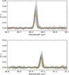 |
Fig. 1 Observed spectra after baseline removal for the second observation window (February 2012) at 66.44 μm (top) and 67.09 μm (bottom). The spectra are presented as line-to-continuum ratio minus one. The scatter in the peak position of the line is mainly due to Doppler shift induced by Saturn’s rapid rotation. For both observations, all the plotted spectra correspond to the pointings selected within the planetary disc, as shown with the black dots on Fig. 2 second row (i.e. second observation window). |
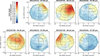 |
Fig. 2 Water line area maps expressed in units of μm×% of continuum. The four observation time windows are July 2011 at 67.09 μm, February 2012 at 66.44 and 67.09 μm, July–August 2012 at 66.44 and 67.09 μm, and January–February 2013 at 66.44 and 67.09 μm. Saturn’s 1-bar level is represented by the black ellipse, with the north pole facing upwards. A selection of iso-latitudes are plotted with grey lines. The rotation axis corresponds to the thin dashed black line. The beam spatial extent is illustrated by the circle in a dashed blue line. The black dots correspond to the central position of the spatial pixels. The position and extension of the beacon (see Table 3) at mid-observation time is represented with the thick dashed black lines. A cubic interpolation was applied to the data. |
3 Modelling
We modelled the spectroscopic observations with the line-byline radiative transfer model described in Cavalié et al. (2019), which accounts for the 3D ellipsoidal geometry of the planet and the emission/absorption of the rings. Saturn’s rotation (9.87 km s−1 at the equator) induces longitudinal smoothing of the beacon emission over 51° and 31°, respectively, during the 1.5 hour integration time for the first window and 54 minutes for the other windows. It is taken into account by averaging the radiative transfer results at the start, mid and end observation time. Several inputs are necessary in the model: the 3D temperature and background composition fields, the geometry and orientation of the planet with respect to Herschel, the position of the beacon at the time of the observations, and the water spatial distribution.
3.1 Temperature fields
3.1.1 Background temperature field
For the background thermal field (i.e. without the beacon), we used the altitude-latitude seasonal field derived by Fletcher et al. (2018) from the entire set of low-spectral-resolution (15 cm−1) Cassini/CIRS observations. For each of our observations, we extracted the field at the relevant date. Each zonal field was then re-gridded on a regularly spaced latitude-longitude grid (5°×5°) at each pressure level using linear interpolation.
3.1.2 Temperatures in the beacon region
In the latitudinal and longitudinal region where the presence of the beacon alters the temperature field, we replaced the data of our background thermal field by relevant retrievals performed as close as possible in time to our observations. We interpolated linearly at the latitude and longitude boundaries the temperatures between the background and beacon retrievals to smooth the whole thermal field for each date.
For our first two observation windows (July 2011 and February 2012), we took the beacon temperatures retrieved by Fletcher et al. (2012) from July 7, 2011 and January 27, 2012 Cassini/CIRS observations. These are the closest dates to our observations and, given the long radiative timescales of several weeks in Saturn’s stratosphere, we assumed no temperature changes within the beacon over the short difference in time between the Cassini/CIRS and the Herschel/PACS observations (i.e. ≈ a week). The July 72011 temperature field consists of a longitudinal section centred at the beacon latitude (see Fig. 3a). The altitudinal coverage encompasses the upper troposphere and the stratosphere. We deduced the latitudinal extension of the beacon from the IRTF/TEXES observations of Fouchet et al. (2016). The January 27, 2012 temperature field consists of latitudinal and longitudinal sections centred on the beacon (see Fig. A.1).
For our last two windows (July–August 2012 and January–February 2013), we used temperature retrievals from similar, as-of-yet unpublished, Cassini/CIRS data obtained on August 162012 and January 5 2013. As opposed to the other dates, we have no information regarding the latitudinal extent of the beacon in January 2013, since no latitudinal coverage was performed with Cassini/CIRS between August 2012 and October 2014. We assumed the same latitudinal extent as in the 2012 data. All the beacon region thermal fields that we used to reconstruct a full 3D field for each observation are presented in Fig. A.1.
CIRS spectra were latitudinally averaged between 25–44°N (planetocentric) to increase the S/N in the inversions. These averaged spectra were then used to retrieve the four longitudepressure fields taken on July 7, 2011, January 27, 2012, August 16, 2012, and January 5, 2013. A similar approach was used for the two latitude-pressure fields taken on January 272012 and August 16, 2012, with a longitudinal average around the beacon centre between 195–225°W and 90–110°W, respectively. The resulting thermal fields thus lack detailed information on the horizontal structure because of the latitudinal and/or longitudinal averaging. The initial information on the horizontal details cannot be recovered; nor can the uncertainty and fluctuations on the pre-average variations. The temperatures close to the beacon centre are underestimated, while the temperatures further away of the beacon centre are overestimated with the averaging. However, the overall effect should be compensated for, mostly because the Planck function varies linearly with the temperature in our frequency domain, and the thermal field is smoothed out. The beacon being smaller than the PACS beam size, we only look at the larger scales. Uncertainties on the temperature field of the order of 2 K are estimated at the pressure levels of interest (several millibar) from the temperature retrievals and from the fluctuations arising from the time gap between the CIRS data and our PACS data.
The vertical profiles at the central latitude and longitude of the beacon, retrieved from the aforementioned Cassini/CIRS observations of July 7, 2011, January 27, 2012, August 16, 2012, and January 52013 are displayed in Fig. 3b. They are compared to a quiescent conditions profile obtained at the same latitude in January 22011 a few weeks after the onset of the storm. Fig. 3b additionally displays the warmest temperature profile measured by CIRS as it was used in the photochemical model of Moses et al. (2015). This thermal profile was retrieved on May 42011 from Cassini/CIRS spectra averaged around the beacon centre (±10° average in longitude and ±5° in latitude, Fletcher et al. 2012).
The temperature peak in the beacon corresponds to a temperature increase over quiescent conditions of 67 K, 62 K, 53 K, and 36 K, respectively for the four observation periods. It is obvious that the stratosphere had not returned to quiescent conditions even two years after the storm onset. We also note that we simply extrapolate isothermally the temperatures from the 0.2 mbar level up to the top of the stratosphere as shown in Fig. 3c, because these levels are not well constrained by Cassini/CIRS, particularly using the low-spectral-resolution nadir observations of Fletcher et al. (2012). The two water lines analysed in this paper are not sensitive to these high levels anyway (see the water contribution functions on Fig. 7).
As the beacon travels at a given drift rate and the above fields are not measured at the same time as our Herschel observations, the final step when building the thermal fields is to shift them in longitude accordingly (see next section).
3.1.3 Beacon drift rate
Fletcher et al. (2012) observed that the beacon drifted in longitude at a rate of (2.70 ± 0.04)° day−1 (or −26.4 ± 0.4 m s−1 at 35°) from July 2011 to March 2012. It is thus an important point to consider when building the thermal fields for our analysis, because the Cassini/CIRS observations presented in Section 3.1.2 were not recorded at the same date as our Herschel/PACS data. Consequently, we must account for this drift to have the beacon properly located in longitude in the thermal fields we use for the radiative transfer analysis. For the July 2011 and January 2012 thermal fields, we applied the beacon drift rate derived by Fletcher et al. (2012) which is valid for our first two windows, and corrected the beacon centre longitude. The resulting field for the July 2011 window is shown in Fig. 3c as an example.
Beyond March 2012, the beacon drift rate remained unconstrained. We thus analysed unpublished CIRS thermal fields similar to those presented in Fletcher et al. (2012) to derive an updated drift rate over time. The entire Cassini/CIRS dataset used is presented in Fig. B.1. The temperatures are derived from CH4 emission averaged between 1280 and 1320 cm−1 and therefore sensitive to stratospheric temperatures averaged over the millibar levels. The data correspond to a latitudinal average between 25 and 44°N, and thus cover the beacon latitudinal centre. They extend from 2010 (i.e. before the storm onset) to the end of 2014 (i.e. ~2 years after our last Herschel/PACS observation window), so we have an overall panorama of the entire storm event in the stratosphere at the millibar levels as a function of time and longitude. For each of the dates after the merging in April–May 2011 (we only look at the evolution of the merged beacon), we identified the central longitude of the beacon as the middle of the thermal bell-shaped curve, which is rather symmetrical with respect to the middle longitude. We did not use the maximum temperature peak in the beacon region as an estimator of the beacon centre because of the variability of the maximum location with time, and also because of the uncertainty on the temperature retrieval from inversion models (2–3 K, Fletcher et al. 2012). To illustrate this point, the determination of the beacon centre on July 7, 2011 from the temperature peak (see Fig. 3a) would be complex as the region of maximal temperature at around 190 K is really extended with longitude (about 50°). The beacon central longitude over time estimated from the previous method is summed up in Fig. 4. We find a beacon drift velocity of (3.02 ± 0.01)°.day−1 (or −29.4 ± 0.1 m s−1 at 35°N) beyond March 2012. The thermal fields of our last two Herschel/PACS windows (July–August 2012 and January–February 2013) were corrected using this new drift rate.
The increase in the drift rate between the two periods is difficult to explain owing to the lack of wind field measurements in the stratosphere of Saturn over the lifetime of the beacon at the relevant pressure levels. We note, however, that the retrograde motion of the beacon is consistent with two independent direct wind measurements performed with ALMA in the millibar layers. Cavalié et al. (2024a) measure (−33 ± 18) m s−1 between 30°N and 45°N in data taken with ALMA in January 2012. Stratospheric wind measurements performed in May 2018, also with ALMA, at the beacon latitudes by Benmahi et al. (2022) indicate as well retrograde winds, with a wind velocity of (−50±20) ms−1.
With the knowledge of the beacon central position over time, we retrieved the longitudinal extension of the beacon over time (see Fig. B.1, middle and right panels) from the above data. We applied a longitudinal shift of the thermal fields of Fig. B.1 (left panel), according to the results of Fig. 4, to align the beacon at 180° W over time. Fig. B.1 (right panel) results from a bilinear interpolation of the aligned data of the left panel and shows the beacon extension over time at the millibar levels. The thermal signature of the beacon is seen up to the end of 2013 at these levels and returns to quiescent conditions.
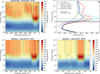 |
Fig. 3 (a and b) Temperature fields at an averaged latitude of 35°N retrieved from Cassini/CIRS observations by Fletcher et al. (2012). (a) Pressurelongitude cut for July 7, 2011. (b) Vertical profiles extracted from the July 7, 2011, January 27, 2012, August 16, 2012, and January 5, 2013 thermal fields (see Fig. A.1). The coloured lines are taken at the central longitude of the beacon. The central longitude is defined following the beacon drift presented in Section 3.1.3. The dashed black line represents the quiescent conditions (taken here on January 2, 2011) at the early stages of the storm. The May 4, 2011 hot beacon core temperature profile is depicted by the dashed sky-blue line and was used in the photochemical model of Moses et al. (2015). The horizontal lines represent the water condensation level calculated using Fray & Schmitt (2009) for each temperature profile (same colour and line code for a given date). (c and d) Final thermal fields used in our radiative transfer calculations for the first window (July 12, 2011), constructed from the above Cassini/CIRS data and the background seasonal data from Fletcher et al. (2018). An isothermal extrapolation from 0.2 mbar to the top of the atmosphere was performed. (c) Similar to (a) at 35°N, after the beacon drift was accounted for. (d) Pressure-latitude constructed field at 50°W. |
Observation geometry of Saturn for the various epochs at mid-observation.
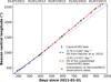 |
Fig. 4 Central longitude of the beacon through time. The black dots are derived from the Cassini/CIRS thermal fields averaged on the 25–45°N latitudinal band, i.e. for an average latitude of 35°N, at the millibar level in the stratosphere. Data points are derived from the longitudinal centre position of the beacon, calculated as the middle of the longitude-temperature curve, which is rather symmetric with respect to the middle longitude. The dashed blue line represents the trend from Fletcher et al. (2012) between July 2011 and March 2012. The dashed red line shows the trend after March 2012 derived in this paper. The dotted lines correspond to the extrapolation of the two trends. The vertical grey line delimits the two temporal periods. The interpolation at our Herschel/PACS observations dates are represented by the green x-shaped points. |
3.2 Observation geometry
We retrieved the observation geometry of Saturn from JPL/Horizons for the different observation times. These data, which are essential for extracting the appropriate temperature information from the full 3D thermal fields and then analysing the maps with radiative transfer calculations, are contained in Table 2. In this paper, all latitudes (φ) are planetocentric, and all longitudes (λ) are System III longitudes.
The beacon geometrical data considered in this paper (see Table 3) have been derived from the observations presented in Fletcher et al. (2012), and which cover our first two observation windows. For the last two windows, we used the unpublished thermal mapping observations of August 162012 and January 5, 2013 presented in Fig. A.1, and accounting for the drift rate of Section 3.1.3. For the 2013 data, we assume a beacon latitudinal extent identical to that seen in the 2012 data as the latitude-pressure field was not measured on this date.
3.3 Composition
3.3.1 Background composition
We started from the background atmospheric composition described in Cavalié et al. (2019) regarding H2, He, CH4, NH3, and PH3. We also adopted the empirical distribution for stratospheric H2O they derived from Herschel/PACS observations of January 2011. The H2O mole fraction at the millibar level varies with latitude following a Gaussian distribution centred on the equator of Saturn, as follows:
![Mathematical equation: $\[y_{\mathrm{H}_2 \mathrm{O}}(\Phi)=y_{\mathrm{eq}} \times \exp \left(-\frac{\Phi^2}{2 \sigma^2}\right)\]$](/articles/aa/full_html/2025/06/aa53029-24/aa53029-24-eq2.png) (1)
(1)
with yH2O the water mole fraction, Φ the planetocentric latitude, yeq = 1.1 ppb the water mole fraction at the equator, and σ = 25°. At a given latitude, yH2O was set to be constant for pressures lower than the water condensation level computed according to the thermal fields and the saturation law published by Fray & Schmitt (2009). Examples of this background field are illustrated in Fig. 5 at several latitudes.
This water vapour originates from an external flux coming from the torus of water vapour fed by the plumes of Enceladus (Hansen et al. 2006; Porco et al. 2006; Waite et al. 2006; Hartogh et al. 2011; Cassidy & Johnson 2010), which diffuses vertically from the top of the atmosphere until it reaches the top of the water cold trap. The cold trap extends from 20 bar in the troposphere (Cavalié et al. 2024b) to ~2 mbar in the stratosphere in quiescent conditions (see Fig. 3b). This upper boundary of the cold trap varies with latitude because of the thermal field. At this level, the water vapour from the external flux condenses and is expected to form the stratospheric water haze (Moses et al. 2000; Ollivier et al. 2000).
Beacon geometry data at the time of the Herschel/PACS observations.
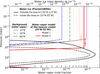 |
Fig. 5 Profiles of the water vapour mole fraction (bottom x scale) and the water ice mass density (top x scale) as a function of pressure. The water vapour profiles are extracted from the water 3D field of July 12 2011. The solid purple line, the dashed-dotted green line and the dashed blue line depict the background field derived from Cavalié et al. (2019) at, respectively, 15,50, and 60°N. The thin vertical dashed lines represent the values of the water vapour mole fraction at ~1–2 mbar found in Cavalié et al. (2019) in quiescent conditions, as a function of latitude. The latitudes are labelled vertically at the bottom of the graph. Model 1 (dotted orange line) indicates the water profile of Step 1 (see Section 4.1) in which we keep the pre-storm water field of Cavalié et al. (2019) to test the enhancement of the water line amplitude due to temperature increase only. The red line shows the best fit of Model 3 (i.e. Step 3, Section 4.3) for July 2011, in which we vary the water mole fraction in the beacon. The orange and dark red bars represent the vertical sensitivity range from the water contribution functions, corresponding to the Step 1 and Step 3 models, respectively (see also Fig. 7). The crosses correspond to the altitude of maximum contribution to the line. The water ice profiles were computed with the PlanetCARMA cloud model of Barth (2020) adapted to the Saturn stratosphere with the July 122011 thermal profile outside the beacon at 35°N–115°W for the solid black line and inside the beacon at 35°N–55°W for the dashed black line. |
3.3.2 H2O distribution in the beacon
Within the beacon, the temperature dramatically increases during the storm in the pressure range where H2O condensation usually occurs (Fletcher et al. 2011, 2012). This leads to a downward shift of the condensation level as shown in Fig. 3b. As a consequence, there is a whole new region in which H2O could exist in its vapour phase during the lifetime of the beacon. In quiescent conditions, there is no water emission emanating from these layers because of condensation. Thus, the amount of water vapour in these layers had never been characterized before.
Given the long timescales related to eddy mixing in the 1–10 mbar layer (τ = H2/Kzz ~ 200–400 years compared to the few weeks between the onset of the storm and the first Herschel/PACS maps) in quiescent conditions, the effect of vertical mixing should be negligible even if local turbulence may have completely been altered in the beacon. Moses et al. (2015) found that downward winds could explain the abundance increases seen at 2 mbar in C2H2 and C2H6 with Cassini/CIRS (Fletcher et al. 2012). Their best fit to the data was obtained with a Gaussian wind profile peaking at log10(P mbar) = −0.5 (i.e. 0.3 mbar) with a maximum velocity of −10 cm s−1 and a standard deviation of log10(P mbar) = 0.8 (i.e. from 0.05 to 2 mbar). It would then roughly take 3–4 weeks to transport H2O from 0.1 mbar to 2 mbar; that is, to the warmer layers in the beacon. Moses et al. (2015) estimated that the H2O column density would increase by a total factor of 8.5 above the condensation level in the beacon, in which a factor of 2.8 is due to those vertical winds and a factor of 3 accounting for the haze sublimation. The water vertical profiles in the beacon obtained in Moses et al. (2015) from photochemical modelling are illustrated in Fig. 6. These profiles were computed to study the beacon at its hot core stage of May 4 2011.
Our approach consisted of three steps: (1) we first assessed whether the temperature increase in the beacon, combined with the latitudinal distribution from Cavalié et al. (2019), was sufficient to reproduce the observed water maps; (2) we then tested more physical vertical water profiles derived from the photochemical models of Moses et al. (2015); and (3) finally, we determined the column density required to account for the beacon strong emission over time with empirical models. The water vapour contribution function calculations from Step 3 are presented in Fig. 7. They indicate that, in the beacon, the enhanced H2O line emission observed in Fig. 2 can be produced in the new water vapour existence region, within the Step 3 water models. We can thus use the H2O maps to quantify the extra H2O column density in this pressure range.
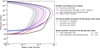 |
Fig. 6 Water vertical profiles as a function of pressure derived from Moses et al. (2015) and from Moses, priv. comm. Their original photochemical profiles are depicted by the thick solid blue, red, and black lines, respectively, in the pre-storm conditions, in the haze sublimation model, and the vertical transport with haze sublimation model. They are derived from a disc-averaged value for the water influx at the top of the atmosphere. As these profiles originate from a disc-averaged observation of water in the stratosphere of Saturn, we first had to rescale the pre-storm profile as a function of latitude following the water distribution found by Cavalié et al. (2019) with an additional fitting factor to reproduce the January 2011 data. The resulting water profiles are plotted in blue at different latitudes. The purple and grey areas represent the best fit results for July 2011 with the two rescaled water models in the beacon. |
4 Results
4.1 Step 1: The effect of the temperature increase
A first model is to consider that no additional water vapour is present in the heated layers during the storm (i.e. no haze sublimation and/or no downwelling winds filling the layers). This model will be referred to as Step 1. The water abundance field in this model is the same as in the pre-storm conditions presented in Fig. 5 and Section 3.3.1. With this model, we only account for the effect of the local temperature increase on water line emission for the layers above the typical condensation level (see Fig. 3b), coupled with the contribution to the line of the water abundance field in quiescent conditions found in Cavalié et al. (2019) in January 22011.
The modelled and the residual maps (which corresponds to the difference between the observed maps of Fig. 2 and the modelled maps of Fig. 8, top left panel) are shown in Fig. 8 (first row) as an example for the first window. All seven modelled and residual maps are presented in Fig. C.1. Water emission is enhanced locally around the beacon because of the higher temperatures, as seen on the modelled maps. The χ2/N values, computed within a beam around the beacon region, range from 11 to 23; that is, ~3–5σ. There is a strong lack of water emission around the beacon position within the seven modelled maps, up to 7σ for the first window. To illustrate this point, Fig. 9 shows the result for the spectrum located closest to the beacon centre for the first date. The location of this spectrum is indicated by a cross in Fig. 8.
The increase in temperature alone, coupled with the nominal water abundance field in quiescent conditions, thus fails to reproduce the observed water maps. The Saturn stratospheric water distribution results from the continuous infall of material from the Enceladus torus and the rings. Moses et al. (2000) and Ollivier et al. (2000) estimated the flux of infalling oxygen in the upper atmosphere of Saturn at ≈106 cm−2 s−1. More recent work from Hartogh et al. (2011) found an infalling flux in Saturn’s atmosphere of ≈6×105 cm−2 s−1 from 2009–2010 Herschel observations. After January 2011 and within the beacon, this flux would have continued to diffuse downward from the pre-storm condensation level to the deeper condensation level, enhancing locally the water column density. The typical water column density at the beacon latitude (35°N) in January 2011 is ≈0.3×1015 cm−2 and is not enough to reproduce the storm conditions. The photochemical model of Moses et al. (2015) predicts an increase in the water column by a factor of 8.5. It would take ≈130 years to increase the nominal water column by a factor of 8.5 in the beacon with a constant influx rate of 6×105 cm−2 s−1. This timescale far exceeds the several months gap between the observations of January 2011 and our dataset. We can thus conclude that the enhanced water emission around the beacon position cannot be explained by the supplementary materiel coming from the continuous infall of water in the several months separating the January data and our dataset. Thus, the extra water abundance in the beacon must come from the stratospheric water haze sublimation and/or the effect of vertical downwelling winds. We could not think of other known mechanism that could significantly increase the water abundance in the stratosphere at the millibar level.
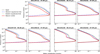 |
Fig. 7 Water contribution functions for each of our seven observations, calculated with the best fit 3D water abundance field in the beacon from Step 3 (see Section 4.3). Dashed black lines refer to a line of sight at the planet disc centre. Dashed-dotted blue lines and dotted green lines correspond to a line of sight at, respectively, the western and eastern equatorial limbs. The solid red lines depict a line of sight at the beacon centre. |
 |
Fig. 8 Modelled line area maps (left) and residual maps (right) for the first window (July 2011) and corresponding to the following models: (first row) Step 1, in which we keep the Gaussian-latitude-dependent profiles of Cavalié et al. (2019) with no water vapour in the beacon new layers delimited by the pre-storm condensation level at 2 mbar and the new condensation level; (second row) Step 3, in which we set the water vapour abundance as a constant free parameter in the beacon to fit the observations. The best fit of July 2011 is presented here. The ‘x’ markers in the maps at RA=−5.9″, Dec=4.2″ (i.e. in the beacon) correspond to the line of sight for which the observed and modelled spectra are shown in Fig. 9. The contours in the residuals are given in units of σ. The solid contours refer to positive residuals and the dashed contours indicate negative residuals. The results for the six other dates are presented in Fig. C.1 for Step 1, and Fig. D.1 for Step 3. |
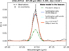 |
Fig. 9 Example of observation and models of the water line at 67.09 μm at the centre of the beacon in July 2011, at the relative pointing coordinates RA=−5.90″, Dec=4.16″ (corresponding to the x-marker position in Fig. 8). The spectrum is expressed in terms of continuum-substracted line-to-continuum (1/c-1). The observed spectrum is in dashed grey lines. It is obtained after the calibration and baseline removal steps presented in Section 2.2. The dashed-dotted green line corresponds to a model in which only the temperature increase in the beacon is accounted for (Step 1 – see Section 4.1). The solid blue line and dotted cyan line represent the rescaled photochemical models (Step 2 – see Section 4.2) in which we consider only the haze sublimation (rescaled by a factor of 0.39), then we add the downward winds to the sublimation (rescaled by a factor of 0.13), respectively. The red line depicts a model in which the water mole fraction is fitted in the beacon as a single free parameter (Step 3 – see Section 4.3). The black point with error bars corresponds to the 1σ line amplitude uncertainty of about 15–20%, mostly caused by the baseline removal. This value is different from the line area uncertainty (see 2Section 2.2). |
4.2 Step 2: Photochemical models
The exceptional increase in temperature alone is not sufficient to explain the observed line areas. We thus need to add an extra amount of water vapour to increase the water emission in our radiative transfer calculations. In this section, we explore two different water vertical profiles in the beacon based on the photochemical and transport coupled models of Moses et al. (2015). They predict a factor-3 increase in water column density from the haze sublimation and a factor-2.8 increase from vertical transport (see Section 3.3.2) in the hot beacon core of May 42011 compared to their mid-2010 pre-storm conditions. A total increase in the water column by a factor of 8.5 is thus predicted by their model. Haze sublimation alone is tested first in the beacon in Section 4.2.2, then the vertical downwelling winds are added in Section 4.2.3. The vertical profiles, taken from Moses et al. (2015), are presented in Fig. 6. The general method to adjust these profiles in our radiative transfer calculations is discussed in Section 4.2.1.
4.2.1 Building the water vapour 3D-field
The water vertical profiles can only be tested on our first observation window (July 12, 2011) which is the closest in time to the hot beacon core stage of May 4, 2011 on which the work of Moses et al. (2015) is based. The thermal field changed between the two dates, but the maximal temperature difference of 20 K is located at 2 mbar, a pressure level well above the new condensation level. This difference at 2 mbar has thus no impact on the water profile. The only important pressure level to consider is the condensation level, whose vertical position influences the vertical range where water can be in the vapour phase. According to Moses et al. (2015), the water condensation level in the hot beacon core lies at ≈9 mbar. This level shifts to ≈12 mbar in July 2011 according to the Fletcher et al. (2012) profiles (see Fig. 3b). A deeper condensation level would eventually lead to an even higher water column density in the beacon if we extend their ‘sublimation’ profile towards the condensation level of July 2011. The dynamic behaviour of the beacon during the 3 months separating the two dates is unknown, but if the vertical downwelling winds profile found in Moses et al. (2015) is still valid in July 2011, we can also expect even more water column in the beacon region from the continuous supply of the upper transport. In a first approximation, we use the profiles of May 2011 to evaluate the physical processes in the beacon in July 2011.
The two water vertical profiles originate from a pre-storm profile obtained from a single disc-averaged observation of water in Saturn’s stratosphere (Moses et al. 2000). Our observations are latitude-dependent and therefore we first need to adapt the photochemical profiles to build a coherent 3D field as a function of latitude. The background 3D field is built in two steps, as follows: (1) the pre-storm profile is rescaled as a function of latitude to match the Gaussian distribution of Equation (1) at 1 mbar, then (2) this global latitude-dependent field is multiplied by a constant factor to fit the water map of January 2 2011. Details on the thermal field, on the observation strategy and geometry for this date are presented in Cavalié et al. (2019). Radiative transfer calculations were performed in the same configuration as in Cavalié et al. (2019), except for the 3D water field. We find a best global fitting factor of 2.1, which is equivalent to multiplying the pre-storm profile by a factor of 1.5 at the equator and by a factor of 0.5 at 35°N. The rescaled vertical profiles at the equator, 35°N and 50°N, are illustrated in Fig. 6. Because we use a single vertical profile for all latitudes, the resulting 3D field does not follow the latitude dependency of the temperature field, which results in varying condensation levels, especially in the beacon where the condensation line was deeper in July 2011 than in May 2011. These vertical profiles are thus no longer physical in the condensation region. This constitutes a limitation to the method of building the background field.
The water column calculated at the beacon latitude (35°N) is (0.91 ± 0.07)×1015 cm−2. Fig. 10 shows the best fit from radiative transfer calculations and the corresponding residuals. Even if the condensation levels are not well represented here as a function of latitude, a good agreement with the January 2011 data is found and thus the background field can be used for the next steps.
The global field outside the beacon is set with this rescaled pre-storm profile for July 2011. Inside the beacon region delimited in latitude and longitude following data found in Table 3, we use the ‘sublimation-only’ or ‘sublimation with vertical winds’ models, and then we rescale the water field in the whole beacon with a fitting factor. We do not perform any Gaussian rescale as a function of latitude to remove the unknown latitude dependency in the beacon.
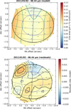 |
Fig. 10 Modelled line area map (top) and residual map (bottom) for the best fit of January 2, 2011 data (Cavalié et al. 2019) with the prestorm model of Moses et al. (2015). The residual map corresponds to the difference between the observed map of Cavalié et al. (2019) (Fig. 2) and the modelled map. The contours are given in units of σ. The solid contours refer to positive residuals and the dashed contours indicate negative residuals. The overall description of the maps is the same as in Fig. 2. |
4.2.2 Sublimation only
We explore in this section the first model of Moses et al. (2015) accounting only for the haze sublimation, with the previous water vapour background 3D-field. The modelled water map as well as the residuals are shown in Fig. 11 (top two panels). The water line emission is enhanced around the beacon position in this model because of two related effects: (1) the increase in temperature in the millibar layers, as in Section 4.1, and (2) the additional water vapour column density resulting from the haze sublimation at a few mbars. The enhanced emission is not centred on the beacon for geometrical reasons, and because of the large beam size and the planet’s rotation during the observing time that spreads out the emission. An example of a modelled spectrum in the beacon is presented in Fig. 9, at the pointing depicted by a blue ‘x’ symbol on Fig. 11. The best fit is obtained for a scaling factor of ![Mathematical equation: $\[0.39_{-0.16}^{+0.21}\]$](/articles/aa/full_html/2025/06/aa53029-24/aa53029-24-eq3.png) with 1σ uncertainties. The corresponding water vertical profile is shown in Fig. 6 with the purple area. The χ2/N value calculated within one beam around the beacon is 1.1. This model gives a good agreement with the observations after the proper rescaling. The column density at the beacon centre (35°N–55°W), calculated from 100 mbar to the top of the atmosphere, is
with 1σ uncertainties. The corresponding water vertical profile is shown in Fig. 6 with the purple area. The χ2/N value calculated within one beam around the beacon is 1.1. This model gives a good agreement with the observations after the proper rescaling. The column density at the beacon centre (35°N–55°W), calculated from 100 mbar to the top of the atmosphere, is ![Mathematical equation: $\[2.0_{-0.8}^{+1.0} \times 10^{15} \mathrm{~cm}^{-2}\]$](/articles/aa/full_html/2025/06/aa53029-24/aa53029-24-eq4.png) with this July 12, 2011 ‘sublimation-only’ model.
with this July 12, 2011 ‘sublimation-only’ model.
4.2.3 Sublimation with vertical winds
We now add the effect of vertical downwelling winds on the water vapour profile. Fig. 11 (bottom panels) presents the radiative transfer results with this second model. A spectrum corresponding to a line of sight in the beacon is given as an example in Fig. 9. The best fit corresponds to a scaling factor of ![Mathematical equation: $\[0.13_{-0.06}^{+0.08}\]$](/articles/aa/full_html/2025/06/aa53029-24/aa53029-24-eq5.png) with 1σ uncertainties and is obtained for a χ2/N value of 1.1 around the beacon. The vertical profile associated with the best fit is illustrated in Fig. 6 with the grey area. The column density computed at the beacon centre is
with 1σ uncertainties and is obtained for a χ2/N value of 1.1 around the beacon. The vertical profile associated with the best fit is illustrated in Fig. 6 with the grey area. The column density computed at the beacon centre is ![Mathematical equation: $\[1.9_{-0.8}^{+1.1} \times 10^{15} \mathrm{~cm}^{-2}\]$](/articles/aa/full_html/2025/06/aa53029-24/aa53029-24-eq6.png) . It is consistent with the rescaled ‘sublimation-only’ model column density. This was expected as we fit the right amount of water vapour in the sensitivity pressure region. The increase ratio between the storm fitted models and the pre-storm fitted model lies between 1.0 and 3.4.
. It is consistent with the rescaled ‘sublimation-only’ model column density. This was expected as we fit the right amount of water vapour in the sensitivity pressure region. The increase ratio between the storm fitted models and the pre-storm fitted model lies between 1.0 and 3.4.
The previous results highlight that a solution is found from two different water vapour vertical profiles, which are derived from different physical assumptions (see Fig. 11). The column densities inferred using the two vertical profiles are essentially the same, at about 2.0×1015 cm−2. From Fig. 6, we see that the fitted profiles from the two models overlap in the altitudinal range from which most of the line emission is formed (see the example of the July 2011 Step 3 sensitivity range in Fig. 7, which is essentially the same here). This confirms that the right amount of water needed to reproduce the observations is fulfilled in this region. However, the two profiles do not match for levels lower than 0.1 mbar, and are also both incoherent with the rescaled background field at 35°N, but we are not sensitive at these high altitudes anyway with our observations.
An extra amount of water vapour in the beacon is expected from vertical winds, as was observed for other molecules. All molecules should be affected similarly by the vertical winds, the only difference with other molecules is that water is a condensable species in the stratosphere, and some water vapour might be added on top of the winds contribution from the haze sublimation. These results show (1) the limitation of our dataset in terms of vertical sensitivity, and (2) the lack of knowledge on the beacon dynamical behaviour and chemical behaviour.
Firstly, the lines are far from being spectrally resolved (the spectral resolution is about 100 times the natural line width). As was shown with the previous results, we cannot retrieve the water vertical profile in the beacon, and multiple solutions are acceptable. What really matters is the amount of water vapour put in the sensitivity region delimited in the altitudinal range from ~1 mbar to ~10 mbar (see the water contribution functions in Fig. 7). The primary conclusion is that, due to the PACS limited spectral resolution, our sensitivity is restricted to a single parameter, the water column density within the beacon. We are also limited by the spatial resolution which is half the planet size, thus it is unnecessary to put a multi-parameter latitudinally dependent model of water in the beacon.
Secondly, we are also limited by our lack of knowledge on the beacon which is a dynamic and time-evolving structure. Our observations are space and time dependent. Important physical variables such as the vertical mixing Kzz, are not constrained as a function of space and time in the beacon. Considering the vertical winds, the water excess transported from above is strongly dependent on the pre-storm water gradient in the stratosphere (see Fig. 6), which in turn depends on Kzz. Moreover, the distribution of water ice particles in the stratospheric haze has never been observed before, which means that the quantity of water stored in this haze (and consequently the quantity released by the sublimation during the storm) can only be estimated with models. The ice distribution depends on the influx of water above the condensation level, on condensation, on the local distribution of aerosols on which water can stick, on coagulation, gravitational settling, evapouration from thermal fluctuations. Then, the evolution of the water vapour present in the new condensation region depends on an equilibrium between sublimation and recondensation, and also depends on the vertical winds. All free parameters and unknowns of complex water models can therefore not be constrained with our spectrally and spatially limited dataset.
In the next section, we propose a simpler approach, in which we only fit a single parameter, the water mole fraction (or, equivalently the water column density) in the beacon as a function of time. Finally, using a cloud model, we give a first estimation of the relative magnitude of sublimation versus vertical winds as the source of the extra water vapour seen in the beacon in Section 5.
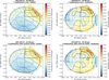 |
Fig. 11 Modelled line area maps (left) and residual maps (right) for the two water models of Moses et al. (2015): a first water profile considering only the sublimation of the water haze in the beacon (top) and a second model in which the vertical downwelling winds are added on top of the haze sublimation (bottom), both in the hot beacon core model of May 4 2011. The two profiles were used only on our first observation window (July 12, 2011) which is the closest water observation to the hot beacon core model. The two profiles were copied uniformly in the beacon region and multiplied by a factor to fit the data. The background water field is derived from the fit of the January 2011 data with the pre-storm profile. The contours are given in units of σ. The solid contours refer to positive residuals and the dashed contours indicate negative residuals. The ‘x’ markers at RA=−5.9″, Dec=4.2″ (i.e. in the beacon) correspond to the line of sight for which the observed and modelled spectra are shown in Fig. 9. The overall description of the maps is the same as in Fig. 2. |
4.3 Step 3: Fitting the water column density in the beacon
In these sets of empirical models, the water mole fraction inside the beacon is set as a free parameter, constant with altitude from the new local condensation level to the top of the atmosphere in the beacon. From the previous sections, we might expect an enhancement of water vapour from haze sublimation and/or vertical winds, which both tend to increase locally the water mole fraction above the new condensation level. We thus extend the empirical profile down to the new condensation level in the beacon. The corresponding contribution functions are displayed in Fig. 7. They show the limited range of pressures (~1–5 mbar) from which the emission is produced; that is, just above the new condensation line in the beacon. The contribution to the line decreases drastically outside this pressure range. We can thus consider the value of the fitted water mole fraction as a fitting data point located at the pressure level where the contribution function peaks, and valid within a range of a few mbars around this peak. The water vertical profile corresponding to the water abundance in the beacon that best fits the first observation window is illustrated as an example in Fig. 5. The extension of this constant profile towards higher altitudes (i.e. typically for pressures lower than 0.1 mbar) has little impact on the water line, because the line is not so sensitive to these high altitudes.
Uncertainties on the thermal field of ±2 K lead to an uncertainty on the location of the condensation level. Its exact position is important for two reasons: (1) we take a constant water mole fraction from the condensation level towards the top of the atmosphere, and (2) we still have some sensitivity down to this level, thus a deeper level means an extra column density contributing to the line. We estimated that the uncertainty on the thermal field leads to an uncertainty of about 30% on the water mole fraction. This uncertainty was added quadratically to the fitting uncertainty.
Radiative transfer calculations and residuals are presented in Fig. D.1 for the best fits for the seven water maps, and as an example for the first window in Fig. 8. The spectrum which corresponds to the best fit is represented in Fig. 9 for a line of sight in the beacon for the first window. The χ2/N values, computed within a beam around the 2D extent of the beacon, are 0.6, 0.7, 1.2, 1.1, 0.4, 1.8 and 2.4, following the time order of Table 1 (July 2011 at 67.09 μm, February 2012 at 66.44 and 67.09 μm, July–August 2012 at 66.44 and 67.09 μm, January–February 2013 at 66.44 and 67.09 μm). The best-fitting water abundances are ![Mathematical equation: $\[0.7_{-0.3}^{+0.3}, 1.1_{-0.5}^{+0.5}, 1.2_{-0.6}^{+0.7}, 1.4_{-0.6}^{+0.8}, 2.1_{-1.0}^{+1.2}, 1.1_{-0.4}^{+0.5}\]$](/articles/aa/full_html/2025/06/aa53029-24/aa53029-24-eq7.png) , and
, and ![Mathematical equation: $\[1.4_{-0.6}^{+0.7} \times 10^{-9}\]$](/articles/aa/full_html/2025/06/aa53029-24/aa53029-24-eq8.png) (1σ uncertainties), respectively. For a given time window, the observations at 66.44 μm and 67.09 μm give results that are compatible within error bars. The differences seen in the nominal values result from the difference in line amplitude. As the 67.09 μm line is 30% less intense than the 66.44 μm one, water line area maps suffer from higher uncertainties at 67.09 μm and therefore a broader range of solutions is possible. The larger uncertainties of the July 2012 derived values are caused by the different observation geometry. The beacon was close to a pure nadir geometry, as opposed to the limb geometry of the other observations, and the observations are thus less sensitive to the water abundance.
(1σ uncertainties), respectively. For a given time window, the observations at 66.44 μm and 67.09 μm give results that are compatible within error bars. The differences seen in the nominal values result from the difference in line amplitude. As the 67.09 μm line is 30% less intense than the 66.44 μm one, water line area maps suffer from higher uncertainties at 67.09 μm and therefore a broader range of solutions is possible. The larger uncertainties of the July 2012 derived values are caused by the different observation geometry. The beacon was close to a pure nadir geometry, as opposed to the limb geometry of the other observations, and the observations are thus less sensitive to the water abundance.
A good agreement between the model and the observations is found for each of the seven maps, but some details are important to notice. First, as mentioned above, the latitudinal extent of the beacon was not known for the last window (January–February 2013). The residual maps at 66.44 and 67.09 μm show a lack of emission in the model towards higher latitudes, but suffer from too strong an emission towards the equator. It probably results from our assumption on the latitudinal extent of the beacon at this point in time. Indeed, we do not have measurements of the temperature as a function of latitude in January–February 2013 and assumed the same latitudinal extent as in August 2012 (see Fig. A.1). We may thus have over/under-estimated the temperature as a function of latitude at the northern and southern edges of the beacon and thus the size of the region in which we vary the water mole fraction. Being closer in time to the end of life of the beacon (see Fig. B.1), it may have been less extended in January–February 2013 than in August 2012. Reducing the latitudinal extension of the beacon and shifting its position towards northern latitudes improve the fits, however the water abundance needed to fit the observations stays relatively the same. It may indicate that the beacon moved towards higher latitudes at the end of its life, but we simply lack the observational constraints to conclude on this point.
In addition, the water vertical profile within the beacon is certainly more complex than the constant water mole fraction profile we adopted in this paper, as shown by the photochemical profiles used in Section 4.2. Our results still give a good estimate on the quantity of water present in the layers of sensitivity (at a few mbars in the beacon) through time. As is shown in Section 4.2, it is unnecessary to make the model more complex with more free parameters because of the limited spatial and spectral resolutions of the observations. Even if the empirical and the photochemical water profiles are based on very different assumptions, the water mole fractions from the two approaches are consistent in the sensitivity layers. While we find a water vapour abundance from an empirical fit of (0.7 ± 0.3)×10−9 for July 2011, the two photochemical models overlaps precisely in this water mole fraction range at several mbars. This conclusion was, again, anticipated as we fill the sensitivity layers with the right amount of water vapour to fit the observations.
Column densities at the beacon centre are plotted over time in Fig. 12 from the previous fitting process. We find, respectively, ![Mathematical equation: $\[2.3_{-0.6}^{+0.7}, 2.9_{-0.7}^{+0.8}, 3.0_{-1.0}^{+1.3}, 3.2_{-1.0}^{+1.3}, 4.5_{-1.6}^{+2.1}, 2.0_{-0.5}^{+0.6}\]$](/articles/aa/full_html/2025/06/aa53029-24/aa53029-24-eq9.png) , and
, and ![Mathematical equation: $\[2.5_{-0.7}^{+0.9}\]$](/articles/aa/full_html/2025/06/aa53029-24/aa53029-24-eq10.png) ×1015 cm−2, following the time order of Table 1. It remains relatively constant (within the error bars) across the monitored time frame, at a mean of (2.5±0.3)×1015 cm−2. The pre-storm column found in January 2011 at 35°N with a similar method of empirical models is
×1015 cm−2, following the time order of Table 1. It remains relatively constant (within the error bars) across the monitored time frame, at a mean of (2.5±0.3)×1015 cm−2. The pre-storm column found in January 2011 at 35°N with a similar method of empirical models is ![Mathematical equation: $\[0.34_{-0.03}^{+0.02} \times 10^{15} \mathrm{~cm}^{-2}\]$](/articles/aa/full_html/2025/06/aa53029-24/aa53029-24-eq11.png) . Using similar empirical models for the water vertical distribution, we find that the water column is enhanced by a mean factor of (7.5±1.6) in the beacon compared to pre-storm conditions at the same latitude. The subtraction of the pre-storm column to the fitted column is also represented in Fig. 12 and shows the extra column density needed to reproduce the enhanced water emission seen in our Herschel/PACS maps.
. Using similar empirical models for the water vertical distribution, we find that the water column is enhanced by a mean factor of (7.5±1.6) in the beacon compared to pre-storm conditions at the same latitude. The subtraction of the pre-storm column to the fitted column is also represented in Fig. 12 and shows the extra column density needed to reproduce the enhanced water emission seen in our Herschel/PACS maps.
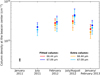 |
Fig. 12 Column density at the beacon centre (35°N and central longitude) as a function of time. The column densities are integrated from ~100 mbar towards the top of the atmosphere. The cross point in January 2011 is derived from the background water field of Cavalié et al. (2019) at 35° N. Darker coloured points relate to the fitting of the observations with a constant water mole fraction in the beacon. Light coloured points refer to the fitted water column density after subtracting the pre-storm column of January 2011, and therefore show the additional column density coming from a combination of vertical winds and sublimation. The red/orange points correspond to the water maps at 66.44 μm and the dark blue/light blue to those at 67.09 μm. |
5 Preliminary cloud modelling
Instrumental limitations prevent us from retrieving the water vertical profile and thus constraining directly the respective contributions of the vertical winds and the haze sublimation to the extra column density we observe in the beacon. But, cloud models, such as the PlanetCARMA (Community Aerosol and Radiation Model for Atmospheres) model (Barth 2020), can be used to try to evaluate the contribution of sublimation. It couples aerosols microphysics and radiative transfer modelling to infer haze formation in a planetary atmosphere and compute, for example, the particle size and mass distributions. Important physical processes at play in hazes, like condensation, evapouration, coagulation, nucleation and sedimentation, are included in this model. More details can be found in Barth (2020).
We have configured this model for this study in two cases prevailing for July 12, 2011 conditions: (i) at the beacon midlatitude but outside the beacon (35°N–115°W), and (ii) at the beacon centre (35°N–55°W). The external water vapour taken as an initial condition at the top of the atmosphere is set as the water mole fraction of the Cavalié et al. (2019) model at the central latitude of the beacon (35°N) in both cases (i) and (ii). This water vapour influx is kept constant until saturation is reached at some point. The water profile then follows the condensation curve. The two model runs are independent and are used here to give an idea of the water ice vertical distribution in quiescent and beacon-like conditions.
Preliminary results obtained for a steady state are presented in Fig. 5. They show both the different altitudes and mass densities of the ice particles in the hazes inside and outside of the beacon at 35°N. The amount of water ice available for sublimation in the beacon is then simply obtained by integrating the difference between the beacon profile and the quiescent one from the condensation level in the beacon upwards; that is, from ~12 mbar (beacon condensation level) to ~2 mbar (quiescent condensation level). The resulting column density of sublimated water is 1.2×1015 cm−2. It corresponds to 45–85% of the extra water vapour column density found at the beacon centre in July 12, 2011, with a nominal value of 60% and 1σ uncertainties derived from the extra column calculations of Step 3 models. These preliminary PlanetCARMA results indicate that haze sublimation could be a significant source of water vapour, which could explain most of the extra water vapour we observe in the beacon.
6 Discussion and conclusion
In this paper, we have presented mapping observations of water vapour in the Saturn stratosphere, recorded by Herschel/PACS between July 2011 and February 2013. These data, taken at a cadence of one dataset every 6 months, and thus covering 18 months, enabled us to monitor the water emission of the hot stratospheric vortex (the ‘beacon’) that was formed in early 2011 as a consequence of Saturn’s Great Storm of 2010–2011. The water vapour maps show significant an increase in the water emission in the regions around the location of the beacon. The peak of emission enhancement is not exactly at the beacon location because of geometrical effects in the build-up of line opacity. A priori knowledge of the temperature fields from independent Cassini/CIRS measurements of Fletcher et al. (2012) pertaining to our observations enables the water abundance in the beacon to be derived from the Herschel observations.
Using radiative transfer modelling coupled to the temperature retrievals, we find that the dramatic temperature increase measured in the 0.5–10 mbar layers within the beacon by Fletcher et al. (2012) with the pre-storm water vapour distribution derived by Cavalié et al. (2019) cannot explain the enhanced water emission recorded by Herschel/PACS. We thus demonstrate that we need to increase the abundance of water vapour locally in the beacon to reproduce the stronger water emission in the observations.
Moses et al. (2015) demonstrated that the local increase in hydrocarbon abundance in the beacon is caused by the presence of vertical transport, and we consider that water vapour was affected in a same way as the rest of the atmospheric species. By analogy to hydrocarbons, we may expect that a part of the additional water vapour needed to reproduce our water maps is caused by the vertical winds. This could constitute a first explanation for the higher emission observed in the beacon.
A possible second source of water at the millibar level is water haze sublimation. Indeed, a stratospheric water haze is expected to exist at pressure levels greater than ~2 mbar from the condensation and accumulation over time of the external flux of water vapour (Moses et al. 2000; Cavalié et al. 2019) coming from Enceladus geysers (Waite et al. 2006; Porco et al. 2006; Hansen et al. 2006), as was predicted by models (Moses et al. 2000; Ollivier et al. 2000). Another source of water vapour could then result from the partial sublimation of the local water haze caused by the important increase in the temperature in the millibar pressure range that implied a downward shift of the condensation level in the beacon. For instance, the condensation level shifted from 2 mbar in early 2011 (pre-storm conditions) to 12 mbar in July 2011 in the beacon. This corresponds to a shift in altitude of the order of 100 km. The total amount of water ice in the haze and the distribution of the ice particles has never been constrained by observations, and thus the amount that sublimated in the beacon is not known a priori.
Unfortunately, we cannot retrieve the water vertical profile in the vertical layers of interest because of the limitations of our dataset in terms of both spectral and spatial resolutions. As a consequence, it is difficult to evaluate the relative magnitude of those two sources. This is best illustrated by the equivalently good fits of July 2011 data obtained with the two rescaled models of Moses et al. (2015) that account for sublimation only, on the one hand, and sublimation and vertical winds, on the other hand.
Using a simpler empirical model, in which we fit a constant water mole fraction above the condensation level in the beacon, we find a relatively constant increase in the water column between July 2011 and February 2013. We derive a mean extra column density of (2.2±0.3)×1015 cm−2, corresponding to an increase over the full temporal coverage of (7.5±1.6) with respect to pre-storm conditions at the beacon latitude. It is worth noting that the temporal increase tentatively seen in the beacon centre column densities in Fig. 12 from July 2011 to July–August 2012 is not significant as the July–August 2012 window suffers from higher uncertainties due to the beacon’s position in nadir geometry. We also remind the reader that the thermal field of the last window in January–February 2013 is not well constrained due to the lack of information about the beacon’s latitudinal extent. The decrease seen in Fig. 12 for the last date is thus not well constrained.
When using physically based profiles following the work of Moses et al. (2015), we find a water column increase of a factor of 1.0–3.4 at 35°N in July 2011. This factor is 2–4 times less than the one found with the empirical model. This is caused by the fact that neither the 66.44 nor the 67.09 μm lines are optically thin. The lines are thus not only abundance-dependent (and therefore column-density-dependent), but also temperaturedependent. As the opacity of the 66.44 μm line is greater than the 67.09 μm line, the 67.09 μm line is more sensitive to the water abundance and column density. A good fit is obtained as long as the right amount of water vapour is put in the sensitivity altitudinal range. This explains the consistent water mole fractions found between the empirical model fitting and the two rescaled storm profiles of Moses et al. (2015) at ~3 mbar (~contribution function peak) in the beacon for July 12, 2011.
The fact that the 66.44 μm line has a stronger opacity than the 67.09 μm one even produces saturation at the line centre. Physical models with stronger gradients and lower abundances in the vicinity of the condensation layer will require more water at the higher-altitude levels to produce the same line area as the empirical model. At some point, the line centre saturates and obtaining a good fit requires one to add more water, in a nonlinear way. Therefore, because of the saturation effect, multiple water columns can lead to the same line area. In addition, there is a discrepancy between the condensation level of the rescaled Moses et al. (2015) pre-storm profile tuned to mid-2010 and the one observed in January 2011. At the beacon latitude of 35°N taken as a reference, it results in too low a condensation level pressure (~1 mbar – see Fig. 6 – vs. ~2 mbar in Cavalié et al. 2019). A much higher fitting factor is then needed to compensate for the emission which is then missing from these deeper levels. Combining these two effects then causes a factor-of-3 discrepancy between the increase factors derived with the two methods (physical vs. empirical models). This point is directly illustrated by our January 2011 pre-storm fitting in Section 4.2.1, in which we find a water column 3 times greater with the rescaled physical model of Moses et al. (2015) than the results of Cavalié et al. (2019) at 35°N that use an empirical model. The global fitting factor found in Section 4.2.1 is thus overestimated to compensate for the emission which is missing from these deeper levels and because of line saturation. With physical models more accurately considering the varying condensation levels with latitude, the line saturation issue at 66.44 μm should be attenuated and we should find a lower pre-storm column density. An increase factor closer to, yet probably not matching, the one found with empirical models should then be found.
The overall constant column seen in Fig. 12 should only be taken as indicative of the continued presence of water vapour in the warmer layers. The temporal evolution of the thermal vertical profile in the beacon after our first observations of July 2011 (see Fig. 3b) shows that the condensation level progressively moves upwards. One could then expect the water vapour of the lower levels to re-condense progressively, leading to a decrease in the column density. The rather constant column over time seen in Fig. 12 could then be caused by the continued effect of the downward winds within the beacon, adding more water vapour from higher levels to the observed ones given the abundance gradient found in the stratosphere in physical profiles such as those of Moses et al. (2015). This effect is difficult to quantify, because the temporal evolution of the downward wind speeds is unconstrained, and from the PACS observations we cannot separate its contribution to the haze sublimation. Thus, further modelling of the 3D dynamical processes in the beacon and of the water haze vertical structure is needed to interpret this extra column density over time.
One solution is to look at cloud models to better constrain the contribution of sublimation. Moses et al. (2015) predicted a factor-3 increase in the water column density from the haze sublimation, which represents 27% of their extra column. In this paper, we used the PlanetCARMA cloud model of Barth (2020) to predict the water ice distribution in the stratospheric haze as a function of altitude in typical atmospheric conditions inside and outside the beacon in the temperature conditions prevailing in July 2011, with the water vapour influx presented in Cavalié et al. (2019). From a preliminary study of the water ice distributions, we obtain as a first estimate that 45–85% of the extra water column seen in July 2011 in the beacon centre could result from the haze sublimation, the rest being caused by the vertical transport of upper material to the millibar levels. The difference between the sublimation profile of Moses et al. (2015) and this study resides in how sublimation and evaporation are handled. The PlanetCARMA model accounts for aerosol microphysics and radiative transfer to produce a more complete picture of the processes occurring in the water condensation region than the parametrized technique used in Moses et al. (2015). Nevertheless, both indicate that haze sublimation plays a significant role in explaining the water abundance increase we derived from the observations.
Three-dimensional time-dependent models of the storm, including the effects of vertical winds, haze sublimation, and recondensation, would help us to more precisely quantify the two counterparts at the origin of the extra column density of water vapour retrieved in the beacon over time. The quantity of water ice stored in the water haze results from an equilibrium between condensation and sedimentation to deeper levels in quiescent conditions. This, in turn, depends on the size and mass of the icy particles. Future work using aerosol microphysical models such as that of Barth (2020) applied to the results of this paper may unveil some of the properties of Saturn’s stratospheric water haze and, more generally, complete our understanding of stratospheric hazes (Guerlet et al. 2015; Fletcher et al. 2023).
Acknowledgements
C. Lefour and T. Cavalié were supported by the Programme National de Planétologie (PNP) of CNRS/INSU and by the Centre National d’Études Spatiales (CNES). PACS has been developed by a consortium of institutes led by MPE (Germany) and including UVIE (Austria); KU Leuven, CSL, IMEC (Belgium); CEA, LAM (France); MPIA (Germany); INAFIFSI/OAA/OAP/OAT, LENS, SISSA (Italy); IAC (Spain). This development has been supported by the funding agencies BMVIT (Austria), ESA-PRODEX (Belgium), CEA/CNES (France), DLR (Germany), ASI/INAF (Italy), and CICYT/MCYT (Spain). The Herschel spacecraft was designed, built, tested, and launched under a contract to ESA managed by the Herschel/Planck Project team by an industrial consortium under the overall responsibility of the prime contractor Thales Alenia Space (Cannes), and including Astrium (Friedrichshafen) responsible for the payload module and for system testing at spacecraft level, Thales Alenia Space (Turin) responsible for the service module, and Astrium (Toulouse) responsible for the telescope, with in excess of a hundred subcontractors. HCSS / HSpot / HIPE is a joint development (are joint developments) by the Herschel Science Ground Segment Consortium, consisting of ESA, the NASA Herschel Science Center, and the HIFI, PACS and SPIRE consortia. L. Fletcher was supported by STFC Consolidated Grant reference ST/W00089X/1. For the purpose of open access, the author has applied a Creative Commons Attribution (CC BY) licence to the Author Accepted Manuscript version arising from this submission. A portion of this work used the ALICE high performance computing facility at the University of Leicester. The authors thank J. Moses for her in-depth review of this paper and for providing the water profiles from her 2015 paper.
Appendix A All Cassini/CIRS thermal fields used
The Cassini/CIRS thermal 3D-fields used in this paper, at the beacon’s central longitude and latitude (only for the two windows of 2012) are illustrated in Fig. A.1.
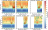 |
Fig. A.1 Thermal fields retrieved from Cassini/CIRS data (Fletcher et al. 2012) and used to build the thermal fields for radiative transfer modelling. The fields shown here only represent the beacon region and its surroundings. They were derived from observations taken within our four Herschel/PACS windows, except that they do not correspond to the same date of observation. The field dates are July 7, 2011, January 27, 2012, August 16 2012, and January 5, 2013. Details on how these fields were retrieved can be found in Section 3.1.2. The first and last dates have longitudinal coverage, and the two intermediate ones have also latitudinal coverage. |
Appendix B Beacon position and extension from Cassini/CIRS fields
The Cassini/CIRS thermal fields used to retrieve the beacon drift rate (Section 3.1.3) are presented in Fig. B.1.
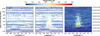 |
Fig. B.1 Left: Thermal fields retrieved from CH4 emission from Cassini/CIRS, averaged between 1280–1320 cm−1, sensitive to the millibar levels in the stratosphere, as a function of longitude and time. The temperatures correspond to an average between 25-45°N in latitude. Data before 2012 are presented in Fletcher et al. (2012), and data after the beginning of 2012 have not been published yet. Middle: Same as the left figure, but after realigning the beacon centre at 180° W in longitude. The performed alignment results in the data points of Fig. 4. The interpolation and smoothing of this figure is illustrated in the right panel to better see the extension of the beacon over time. |
Appendix C Step 1: The effect of temperature increase
The results obtained with the water model of Cavalié et al. (2019) are presented in Fig. C.1 for the seven observation maps.
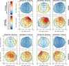 |
Fig. C.1 Modelled H2O water line area maps and residuals obtained within Step 1 (nominal water field of Cavalié et al. 2019), for the seven observation windows. The modelled line area maps are displayed in rows 1 and 3. The units are expressed as μm×% of continuum to directly compare to the observation maps of Fig. 2. The corresponding residual maps are presented in rows 2 and 4 and correspond to the difference between the observed maps of Fig. 2 and the above modelled maps. The contours are given in units of σ. The solid contours refer to positive residuals and the dashed contours indicate negative residuals. The colour scales of the modelled and residual maps are shown on the top left corner. The overall description of the maps is the same as in Fig. 2. |
Appendix D Step 3: Fitting the water column density in the beacon
The results obtained with a model in which we fit the water abundance in the beacon as a constant free parameter above the condensation level, are shown in Fig. D.1 for the seven observation maps.
References
- Barth, E. 2020, Atmosphere, 11, 1064 [Google Scholar]
- Benmahi, B., Cavalié, T., Fouchet, T., et al. 2022, A&A, 666, A117 [NASA ADS] [CrossRef] [EDP Sciences] [Google Scholar]
- Bézard, B., Lellouch, E., Strobel, D., Maillard, J.-P., & Drossart, P. 2002, Icarus, 159, 95 [CrossRef] [Google Scholar]
- Burgdorf, M., Orton, G., van Cleve, J., Meadows, V., & Houck, J. 2006, Icarus, 184, 634 [NASA ADS] [CrossRef] [Google Scholar]
- Cassidy, T. A., & Johnson, R. E. 2010, Icarus, 209, 696 [Google Scholar]
- Cavalié, T., Billebaud, F., Dobrijevic, M., et al. 2009, Icarus, 203, 531 [NASA ADS] [CrossRef] [Google Scholar]
- Cavalié, T., Hartogh, P., Billebaud, F., et al. 2010, A&A, 510, A88 [NASA ADS] [CrossRef] [EDP Sciences] [Google Scholar]
- Cavalié, T., Feuchtgruber, H., Lellouch, E., et al. 2013, A&A, 553, A21 [NASA ADS] [CrossRef] [EDP Sciences] [Google Scholar]
- Cavalié, T., Moreno, R., Lellouch, E., et al. 2014, A&A, 562, A33 [NASA ADS] [CrossRef] [EDP Sciences] [Google Scholar]
- Cavalié, T., Dobrijevic, M., Fletcher, L. N., et al. 2015, A&A, 580, A55 [NASA ADS] [CrossRef] [EDP Sciences] [Google Scholar]
- Cavalié, T., Hue, V., Hartogh, P., et al. 2019, A&A, 630, A87 [NASA ADS] [CrossRef] [EDP Sciences] [Google Scholar]
- Cavalié, T., Benmahi, B., Lefour, C., et al. 2024a, in AAS/Division for Planetary Sciences Meeting Abstracts, 56, 210.06 [Google Scholar]
- Cavalié, T., Lunine, J., Mousis, O., & Hueso, R. 2024b, Space Sci. Rev., 220, 8 [CrossRef] [Google Scholar]
- Coustenis, A., Salama, A., Lellouch, E., et al. 1998, A&A, 336, L85 [NASA ADS] [Google Scholar]
- Dobrijevic, M., Hébrard, E., Loison, J. C., & Hickson, K. M. 2014, Icarus, 228, 324 [NASA ADS] [CrossRef] [Google Scholar]
- Feuchtgruber, H., Lellouch, E., de Graauw, T., et al. 1997, Nature, 389, 159 [Google Scholar]
- Fischer, G., Kurth, W. S., Gurnett, D. A., et al. 2011, Nature, 475, 75 [NASA ADS] [CrossRef] [Google Scholar]
- Fletcher, L. N., Hesman, B. E., Irwin, P. G. J., et al. 2011, Science, 332, 1413 [Google Scholar]
- Fletcher, L. N., Swinyard, B., Salji, C., et al. 2012, A&A, 539, A44 [NASA ADS] [CrossRef] [EDP Sciences] [Google Scholar]
- Fletcher, L. N., Guerlet, S., Orton, G. S., et al. 2017, Nat. Astron., 1, 765 [Google Scholar]
- Fletcher, L. N., Orton, G. S., Sinclair, J. A., et al. 2018, Nat. Commun., 9, 3564 [NASA ADS] [CrossRef] [Google Scholar]
- Fletcher, L. N., King, O. R. T., Harkett, J., et al. 2023, J. Geophys. Res. (Planets), 128, e2023JE007924 [Google Scholar]
- Fouchet, T., Greathouse, T. K., Spiga, A., et al. 2016, Icarus, 277, 196 [NASA ADS] [CrossRef] [Google Scholar]
- Fray, N., & Schmitt, B. 2009, Planet. Space Sci., 57, 2053 [Google Scholar]
- Guerlet, S., Fouchet, T., Vinatier, S., et al. 2015, A&A, 580, A89 [NASA ADS] [CrossRef] [EDP Sciences] [Google Scholar]
- Hansen, C. J., Esposito, L., Stewart, A. I. F., et al. 2006, Science, 311, 1422 [NASA ADS] [CrossRef] [Google Scholar]
- Hartogh, P., Lellouch, E., Crovisier, J., et al. 2009, Planet. Space Sci., 57, 1596 [NASA ADS] [CrossRef] [Google Scholar]
- Hartogh, P., Lellouch, E., Moreno, R., et al. 2011, A&A, 532, L2 [NASA ADS] [CrossRef] [EDP Sciences] [Google Scholar]
- Hesman, B. E., Bjoraker, G. L., Sada, P. V., et al. 2012, ApJ, 760, 24 [Google Scholar]
- Hsu, H.-W., Schmidt, J., Kempf, S., et al. 2018, Science, 362, aat3185 [Google Scholar]
- Lara, L. M., Lellouch, E., González, M., Moreno, R., & Rengel, M. 2014, A&A, 566, A143 [NASA ADS] [CrossRef] [EDP Sciences] [Google Scholar]
- Lellouch, E., Paubert, G., Moreno, R., et al. 1995, Nature, 373, 592 [Google Scholar]
- Lellouch, E., Bézard, B., Moses, J. I., et al. 2002, Icarus, 159, 112 [Google Scholar]
- Lellouch, E., Moreno, R., & Paubert, G. 2005, A&A, 430, L37 [Google Scholar]
- Li, C., Allison, M. D., Atreya, S. K., et al. 2022, in AGU Fall Meeting Abstracts, 2022, P32C-1854 [Google Scholar]
- Mitchell, D. G., Perry, M. E., Hamilton, D. C., et al. 2018, Science, 362, aat2236 [Google Scholar]
- Moreno, R., Lellouch, E., Lara, L. M., et al. 2012, Icarus, 221, 753 [Google Scholar]
- Moreno, R., Lellouch, E., Cavalié, T., & Moullet, A. 2017, A&A, 608, L5 [NASA ADS] [CrossRef] [EDP Sciences] [Google Scholar]
- Moses, J. I., & Poppe, A. R. 2017, Icarus, 297, 33 [Google Scholar]
- Moses, J. I., Lellouch, E., Bézard, B., et al. 2000, Icarus, 145, 166 [Google Scholar]
- Moses, J. I., Fouchet, T., Bézard, B., et al. 2005, J. Geophys. Res., 110, E08001 [Google Scholar]
- Moses, J. I., Armstrong, E. S., Fletcher, L. N., et al. 2015, Icarus, 261, 149 [Google Scholar]
- Ollivier, J. L., Dobrijévic, M., & Parisot, J. P. 2000, Planet. Space Sci., 48, 699 [Google Scholar]
- Ott, S. 2010, in PASP, 434, Astronomical Data Analysis Software and Systems XIX, eds. Y. Mizumoto, K.-I. Morita, & M. Ohishi, 139 [Google Scholar]
- Pilbratt, G. L., Riedinger, J. R., Passvogel, T., et al. 2010, A&A, 518, L1 [NASA ADS] [CrossRef] [EDP Sciences] [Google Scholar]
- Poglitsch, A., Waelkens, C., Geis, N., et al. 2010, A&A, 518, L2 [NASA ADS] [CrossRef] [EDP Sciences] [Google Scholar]
- Porco, C. C., Helfenstein, P., Thomas, P. C., et al. 2006, Science, 311, 1393 [Google Scholar]
- Prather, M. J., Logan, J. A., & McElroy, M. B. 1978, ApJ, 223, 1072 [Google Scholar]
- Sánchez-Lavega, A., del Río-Gaztelurrutia, T., Hueso, R., et al. 2011, Nature, 475, 71 [Google Scholar]
- Sánchez-Lavega, A., Fischer, G., Fletcher, L. N., et al. 2018, in Saturn in the 21st Century, eds. K. H. Baines, F. M. Flasar, N. Krupp, & T. Stallard, 377 [Google Scholar]
- Strobel, D. F., & Yung, Y. L. 1979, Icarus, 37, 256 [Google Scholar]
- Teanby, N. A., Irwin, P. G. J., Sylvestre, M., Nixon, C. A., & Cordiner, M. A. 2022, Plan. Sci. J., 3, 96 [Google Scholar]
- Venot, O., Cavalié, T., Bounaceur, R., et al. 2020, A&A, 634, A78 [NASA ADS] [CrossRef] [EDP Sciences] [Google Scholar]
- Waite, J. H., Combi, M. R., Ip, W.-H., et al. 2006, Science, 311, 1419 [NASA ADS] [CrossRef] [Google Scholar]
- Waite, J. H., Perryman, R. S., Perry, M. E., et al. 2018, Science, 362, 51 [Google Scholar]
All Tables
All Figures
|
Fig. 1 Observed spectra after baseline removal for the second observation window (February 2012) at 66.44 μm (top) and 67.09 μm (bottom). The spectra are presented as line-to-continuum ratio minus one. The scatter in the peak position of the line is mainly due to Doppler shift induced by Saturn’s rapid rotation. For both observations, all the plotted spectra correspond to the pointings selected within the planetary disc, as shown with the black dots on Fig. 2 second row (i.e. second observation window). |
| In the text | |
|
Fig. 2 Water line area maps expressed in units of μm×% of continuum. The four observation time windows are July 2011 at 67.09 μm, February 2012 at 66.44 and 67.09 μm, July–August 2012 at 66.44 and 67.09 μm, and January–February 2013 at 66.44 and 67.09 μm. Saturn’s 1-bar level is represented by the black ellipse, with the north pole facing upwards. A selection of iso-latitudes are plotted with grey lines. The rotation axis corresponds to the thin dashed black line. The beam spatial extent is illustrated by the circle in a dashed blue line. The black dots correspond to the central position of the spatial pixels. The position and extension of the beacon (see Table 3) at mid-observation time is represented with the thick dashed black lines. A cubic interpolation was applied to the data. |
| In the text | |
|
Fig. 3 (a and b) Temperature fields at an averaged latitude of 35°N retrieved from Cassini/CIRS observations by Fletcher et al. (2012). (a) Pressurelongitude cut for July 7, 2011. (b) Vertical profiles extracted from the July 7, 2011, January 27, 2012, August 16, 2012, and January 5, 2013 thermal fields (see Fig. A.1). The coloured lines are taken at the central longitude of the beacon. The central longitude is defined following the beacon drift presented in Section 3.1.3. The dashed black line represents the quiescent conditions (taken here on January 2, 2011) at the early stages of the storm. The May 4, 2011 hot beacon core temperature profile is depicted by the dashed sky-blue line and was used in the photochemical model of Moses et al. (2015). The horizontal lines represent the water condensation level calculated using Fray & Schmitt (2009) for each temperature profile (same colour and line code for a given date). (c and d) Final thermal fields used in our radiative transfer calculations for the first window (July 12, 2011), constructed from the above Cassini/CIRS data and the background seasonal data from Fletcher et al. (2018). An isothermal extrapolation from 0.2 mbar to the top of the atmosphere was performed. (c) Similar to (a) at 35°N, after the beacon drift was accounted for. (d) Pressure-latitude constructed field at 50°W. |
| In the text | |
|
Fig. 4 Central longitude of the beacon through time. The black dots are derived from the Cassini/CIRS thermal fields averaged on the 25–45°N latitudinal band, i.e. for an average latitude of 35°N, at the millibar level in the stratosphere. Data points are derived from the longitudinal centre position of the beacon, calculated as the middle of the longitude-temperature curve, which is rather symmetric with respect to the middle longitude. The dashed blue line represents the trend from Fletcher et al. (2012) between July 2011 and March 2012. The dashed red line shows the trend after March 2012 derived in this paper. The dotted lines correspond to the extrapolation of the two trends. The vertical grey line delimits the two temporal periods. The interpolation at our Herschel/PACS observations dates are represented by the green x-shaped points. |
| In the text | |
|
Fig. 5 Profiles of the water vapour mole fraction (bottom x scale) and the water ice mass density (top x scale) as a function of pressure. The water vapour profiles are extracted from the water 3D field of July 12 2011. The solid purple line, the dashed-dotted green line and the dashed blue line depict the background field derived from Cavalié et al. (2019) at, respectively, 15,50, and 60°N. The thin vertical dashed lines represent the values of the water vapour mole fraction at ~1–2 mbar found in Cavalié et al. (2019) in quiescent conditions, as a function of latitude. The latitudes are labelled vertically at the bottom of the graph. Model 1 (dotted orange line) indicates the water profile of Step 1 (see Section 4.1) in which we keep the pre-storm water field of Cavalié et al. (2019) to test the enhancement of the water line amplitude due to temperature increase only. The red line shows the best fit of Model 3 (i.e. Step 3, Section 4.3) for July 2011, in which we vary the water mole fraction in the beacon. The orange and dark red bars represent the vertical sensitivity range from the water contribution functions, corresponding to the Step 1 and Step 3 models, respectively (see also Fig. 7). The crosses correspond to the altitude of maximum contribution to the line. The water ice profiles were computed with the PlanetCARMA cloud model of Barth (2020) adapted to the Saturn stratosphere with the July 122011 thermal profile outside the beacon at 35°N–115°W for the solid black line and inside the beacon at 35°N–55°W for the dashed black line. |
| In the text | |
|
Fig. 6 Water vertical profiles as a function of pressure derived from Moses et al. (2015) and from Moses, priv. comm. Their original photochemical profiles are depicted by the thick solid blue, red, and black lines, respectively, in the pre-storm conditions, in the haze sublimation model, and the vertical transport with haze sublimation model. They are derived from a disc-averaged value for the water influx at the top of the atmosphere. As these profiles originate from a disc-averaged observation of water in the stratosphere of Saturn, we first had to rescale the pre-storm profile as a function of latitude following the water distribution found by Cavalié et al. (2019) with an additional fitting factor to reproduce the January 2011 data. The resulting water profiles are plotted in blue at different latitudes. The purple and grey areas represent the best fit results for July 2011 with the two rescaled water models in the beacon. |
| In the text | |
|
Fig. 7 Water contribution functions for each of our seven observations, calculated with the best fit 3D water abundance field in the beacon from Step 3 (see Section 4.3). Dashed black lines refer to a line of sight at the planet disc centre. Dashed-dotted blue lines and dotted green lines correspond to a line of sight at, respectively, the western and eastern equatorial limbs. The solid red lines depict a line of sight at the beacon centre. |
| In the text | |
|
Fig. 8 Modelled line area maps (left) and residual maps (right) for the first window (July 2011) and corresponding to the following models: (first row) Step 1, in which we keep the Gaussian-latitude-dependent profiles of Cavalié et al. (2019) with no water vapour in the beacon new layers delimited by the pre-storm condensation level at 2 mbar and the new condensation level; (second row) Step 3, in which we set the water vapour abundance as a constant free parameter in the beacon to fit the observations. The best fit of July 2011 is presented here. The ‘x’ markers in the maps at RA=−5.9″, Dec=4.2″ (i.e. in the beacon) correspond to the line of sight for which the observed and modelled spectra are shown in Fig. 9. The contours in the residuals are given in units of σ. The solid contours refer to positive residuals and the dashed contours indicate negative residuals. The results for the six other dates are presented in Fig. C.1 for Step 1, and Fig. D.1 for Step 3. |
| In the text | |
|
Fig. 9 Example of observation and models of the water line at 67.09 μm at the centre of the beacon in July 2011, at the relative pointing coordinates RA=−5.90″, Dec=4.16″ (corresponding to the x-marker position in Fig. 8). The spectrum is expressed in terms of continuum-substracted line-to-continuum (1/c-1). The observed spectrum is in dashed grey lines. It is obtained after the calibration and baseline removal steps presented in Section 2.2. The dashed-dotted green line corresponds to a model in which only the temperature increase in the beacon is accounted for (Step 1 – see Section 4.1). The solid blue line and dotted cyan line represent the rescaled photochemical models (Step 2 – see Section 4.2) in which we consider only the haze sublimation (rescaled by a factor of 0.39), then we add the downward winds to the sublimation (rescaled by a factor of 0.13), respectively. The red line depicts a model in which the water mole fraction is fitted in the beacon as a single free parameter (Step 3 – see Section 4.3). The black point with error bars corresponds to the 1σ line amplitude uncertainty of about 15–20%, mostly caused by the baseline removal. This value is different from the line area uncertainty (see 2Section 2.2). |
| In the text | |
|
Fig. 10 Modelled line area map (top) and residual map (bottom) for the best fit of January 2, 2011 data (Cavalié et al. 2019) with the prestorm model of Moses et al. (2015). The residual map corresponds to the difference between the observed map of Cavalié et al. (2019) (Fig. 2) and the modelled map. The contours are given in units of σ. The solid contours refer to positive residuals and the dashed contours indicate negative residuals. The overall description of the maps is the same as in Fig. 2. |
| In the text | |
|
Fig. 11 Modelled line area maps (left) and residual maps (right) for the two water models of Moses et al. (2015): a first water profile considering only the sublimation of the water haze in the beacon (top) and a second model in which the vertical downwelling winds are added on top of the haze sublimation (bottom), both in the hot beacon core model of May 4 2011. The two profiles were used only on our first observation window (July 12, 2011) which is the closest water observation to the hot beacon core model. The two profiles were copied uniformly in the beacon region and multiplied by a factor to fit the data. The background water field is derived from the fit of the January 2011 data with the pre-storm profile. The contours are given in units of σ. The solid contours refer to positive residuals and the dashed contours indicate negative residuals. The ‘x’ markers at RA=−5.9″, Dec=4.2″ (i.e. in the beacon) correspond to the line of sight for which the observed and modelled spectra are shown in Fig. 9. The overall description of the maps is the same as in Fig. 2. |
| In the text | |
|
Fig. 12 Column density at the beacon centre (35°N and central longitude) as a function of time. The column densities are integrated from ~100 mbar towards the top of the atmosphere. The cross point in January 2011 is derived from the background water field of Cavalié et al. (2019) at 35° N. Darker coloured points relate to the fitting of the observations with a constant water mole fraction in the beacon. Light coloured points refer to the fitted water column density after subtracting the pre-storm column of January 2011, and therefore show the additional column density coming from a combination of vertical winds and sublimation. The red/orange points correspond to the water maps at 66.44 μm and the dark blue/light blue to those at 67.09 μm. |
| In the text | |
|
Fig. A.1 Thermal fields retrieved from Cassini/CIRS data (Fletcher et al. 2012) and used to build the thermal fields for radiative transfer modelling. The fields shown here only represent the beacon region and its surroundings. They were derived from observations taken within our four Herschel/PACS windows, except that they do not correspond to the same date of observation. The field dates are July 7, 2011, January 27, 2012, August 16 2012, and January 5, 2013. Details on how these fields were retrieved can be found in Section 3.1.2. The first and last dates have longitudinal coverage, and the two intermediate ones have also latitudinal coverage. |
| In the text | |
|
Fig. B.1 Left: Thermal fields retrieved from CH4 emission from Cassini/CIRS, averaged between 1280–1320 cm−1, sensitive to the millibar levels in the stratosphere, as a function of longitude and time. The temperatures correspond to an average between 25-45°N in latitude. Data before 2012 are presented in Fletcher et al. (2012), and data after the beginning of 2012 have not been published yet. Middle: Same as the left figure, but after realigning the beacon centre at 180° W in longitude. The performed alignment results in the data points of Fig. 4. The interpolation and smoothing of this figure is illustrated in the right panel to better see the extension of the beacon over time. |
| In the text | |
|
Fig. C.1 Modelled H2O water line area maps and residuals obtained within Step 1 (nominal water field of Cavalié et al. 2019), for the seven observation windows. The modelled line area maps are displayed in rows 1 and 3. The units are expressed as μm×% of continuum to directly compare to the observation maps of Fig. 2. The corresponding residual maps are presented in rows 2 and 4 and correspond to the difference between the observed maps of Fig. 2 and the above modelled maps. The contours are given in units of σ. The solid contours refer to positive residuals and the dashed contours indicate negative residuals. The colour scales of the modelled and residual maps are shown on the top left corner. The overall description of the maps is the same as in Fig. 2. |
| In the text | |
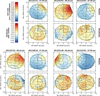 |
Fig. D.1 Same as C.1 but for Step 3 (water mole fraction fitting in the beacon). |
| In the text | |
Current usage metrics show cumulative count of Article Views (full-text article views including HTML views, PDF and ePub downloads, according to the available data) and Abstracts Views on Vision4Press platform.
Data correspond to usage on the plateform after 2015. The current usage metrics is available 48-96 hours after online publication and is updated daily on week days.
Initial download of the metrics may take a while.