| Issue |
A&A
Volume 697, May 2025
|
|
|---|---|---|
| Article Number | A36 | |
| Number of page(s) | 35 | |
| Section | Astrophysical processes | |
| DOI | https://doi.org/10.1051/0004-6361/202452863 | |
| Published online | 06 May 2025 | |
Prospects for optical detections from binary neutron star mergers with the next-generation multi-messenger observatories
1
Gran Sasso Science Institute (GSSI), I-67100, L’Aquila, Italy
2
INFN, Laboratori Nazionali Del Gran Sasso, I-67100, Assergi, Italy
3
INAF – Osservatorio Astronomico d’Abruzzo, 64100, Teramo, Italy
4
Department of Astronomy and Astrophysics, The Pennsylvania State University, University Park, PA, 16802, USA
5
Dipartimento di Fisica, Università di Trento, Via Sommarive 14, 38123 Trento, Italy
6
INFN-TIFPA, Trento Institute for Fundamental Physics and Applications, Via Sommarive 14, I-38123 Trento, Italy
7
GEPI, Observatoire de Paris, PSL University, CNRS, Meudon, France
8
Institut für Kernphysik, Technische Universität Darmstadt, Schlossgartenstr 2, Darmstadt 64289, Germany
9
Department of Physics and Astronomy, University of North Carolina at Chapel Hill, Chapel Hill, NC 27599-3255, USA
10
Joint Space-Science Institute, University of Maryland, College Park, MD 20742, USA
11
Department of Astronomy, University of Maryland, College Park, MD 20742, USA
12
Astrophysics Science Division, NASA Goddard Space Flight Center, Mail Code 661, Greenbelt, MD 20771, USA
13
Institut für Theoretische Astrophysik, ZAH, Universität Heidelberg, Albert-Ueberle-Straße 2, 69120 Heidelberg, Germany
⋆ Corresponding authors: This email address is being protected from spambots. You need JavaScript enabled to view it.
; This email address is being protected from spambots. You need JavaScript enabled to view it.
; This email address is being protected from spambots. You need JavaScript enabled to view it.
Received:
4
November
2024
Accepted:
18
March
2025
Abstract
Context. Next-generation gravitational wave (GW) observatories, such as the Einstein Telescope (ET) and Cosmic Explorer, will observe binary neutron star (BNS) mergers across cosmic history, providing precise parameter estimates for the closest ones. Innovative wide-field observatories, such as the Vera Rubin Observatory, will quickly cover large portions of the sky with unprecedented sensitivity to detect faint transients.
Aims. This study aims to assess the prospects for detecting optical emissions from BNS mergers with next-generation detectors, considering how uncertainties in neutron star (NS) population properties and microphysics may affect detection rates, while developing realistic observational strategies by ET operating with the Rubin Observatory.
Methods. Starting from BNS merger populations exploiting different NS mass distributions and equations of state (EOSs), we modelled the GW and kilonova (KN) signals based on source properties. We modelled KNe ejecta through numerical-relativity informed fits, considering the effect of prompt collapse of the remnant to black hole and new fitting formulas appropriate for more massive BNS systems, such as GW190425. We included optical afterglow emission from relativistic jets consistent with observed short gamma-ray bursts. We evaluated the detected mergers and the source parameter estimations for different geometries of ET, operating alone or in network of current or next-generation GW detectors. Finally, we developed target-of-opportunity strategies to follow up on these events using Rubin and evaluated the joint detection capabilities.
Results. ET as a single observatory enables the detection of about ten to a hundred KNe per year by the Rubin Observatory. This improves by a factor of ∼10 already when operating in network with current GW detectors. Detection rate uncertainties are dominated by the poorly constrained local BNS merger rate, and depend to a lesser extent on the NS mass distribution and EOS.
Key words: astroparticle physics / equation of state / gravitational waves
© The Authors 2025
 Open Access article, published by EDP Sciences, under the terms of the Creative Commons Attribution License (https://creativecommons.org/licenses/by/4.0), which permits unrestricted use, distribution, and reproduction in any medium, provided the original work is properly cited.
This article is published in open access under the Subscribe to Open model. This email address is being protected from spambots. You need JavaScript enabled to view it. to support open access publication.
1. Introduction
Coalescencing binary neutron star (BNSs) are primary astrophysical sources of gravitational wave (GWs) detectable by ground-based detectors. The matter ejected during BNS mergers is neutron-rich and provides the optimal conditions to trigger rapid neutron-capture nucleosynthesis (r-process), giving origin to heavy unstable nuclei (e.g. Eichler et al. 1989; Freiburghaus et al. 1999). The radioactive decay of these nuclei powers a quasi-thermal optical transient known as kilonova (KN). KN emission is intrinsically faint with peak luminosity around 1039−1042 erg s−1, rapidly evolving within days, and characterised by a distinct colour evolution from ultraviolet/blue to red/near-infrared (NIR), (e.g. Li & Paczyński 1998; Kulkarni 2005; Metzger et al. 2010; Kasen et al. 2013; Barnes & Kasen 2013; Grossman et al. 2014; Metzger 2019). The epochal discovery of the GW signal from the BNS merger GW170817 and the detection of its associated optical counterpart (Abbott et al. 2017a, b), AT2017gfo, provided the first direct evidence that BNS mergers produce KN emission and firmly demonstrated that these events are one of the main channels of heavy element formation in the Universe (e.g. Pian et al. 2017; Smartt et al. 2017). The detection of AT2017gfo made it possible to identify the BNS host galaxy. The galaxy recession velocity used along with the distance to the source estimated from the GW signal provided a new way to estimate the local expansion rate of the Universe (Abbott et al. 2017c). The EOS of dense matter has a direct imprint on the GW signal, as well as on the properties of the ejected material. The latter eventually shapes the KN emission making the joint observation of GWs and KN signals a powerful tool for unveiling the nature of matter in neutron star (NSs) (see e.g. Margalit & Metzger 2017; Dietrich et al. 2020; Breschi et al. 2021, 2024). Several factors played a key role in the successful detection of AT2017gfo and its identification as the counterpart of the GW signal; the precise localisation in the sky (∼28 deg2) provided by the LIGO and Virgo network, the relatively small distance (40 Mpc) that enabled to identify candidate host galaxies, the timely and effective follow-up by ultraviolet, optical and NIR telescopes, and finally the extensive photometric and spectroscopic observational campaign to characterize the candidate KN. The characterization campaign identified distinct colour evolution and broad absorption features consistent with the presence of neutron-capture elements.
In 2019, a second GW signal from the inspiral phase of a BNS merger was detected, named GW190425 (Abbott et al. 2020a). Despite the extended follow-up efforts, no electromagnetic (EM) counterparts were identified mainly due to the poorly constrained sky localisation of the event (≃104 deg2). This event was particularly interesting in itself because of its chirp mass (1.44±0.02 M⊙) and total mass between 3.3 M⊙ and 3.7 M⊙, which are significantly larger than that of any other BNS system in the Milky Way. Several theoretical studies have since explored the expected EM emission from events similar to GW190425, either considering high-mass BNS or neutron star-black hole (NS-BH) binaries with a low-mass black hole (BH) (Kyutoku et al. 2020; Raaijmakers et al. 2021a; Barbieri et al. 2021; Camilletti et al. 2022; Dudi et al. 2022; Radice et al. 2024).
Although GW170817 has shown the great potential and impact that such multi-messenger events have on several fields of physics, from relativistic astrophysics to cosmology and nuclear physics, it remains a one-occurrence event. No significant low-latency BNS candidates have been reported in the fourth run of LIGO, Virgo and KAGRA (Akutsu et al. 2019) (LVK) observations. However, it is noteworthy to report that two long gamma-ray burst (GRBs), GRB 211211A (Rastinejad et al. 2022; Troja et al. 2022; Mei et al. 2022) and GRB 230307A (Levan et al. 2024; Yang et al. 2024), at a distance within the reach of the current GW detectors, were detected showing KN emission signatures that demonstrated their origin from the coalescence of NS-NS or NS-BH binaries. They were observed while GW detectors were undergoing upgrades.
Upcoming observational campaigns of the Advanced GW detectors LIGO, Virgo, KAGRA, and LIGO-India (Bailes et al. 2021) are expected to detect between a few up to several hundred BNS mergers per year up to redshift z∼0.2 (Abbott et al. 2020b; Petrov et al. 2022). The next-generation GW observatories, such as Einstein Telescope (ET) and Cosmic Explorer (CE), are expected to significantly increase the detection rates, identifying up to 105 BNS mergers per year, and expand the observable horizon to z∼4 with ET (Branchesi et al. 2023) and z∼10 with (CE) (Evans et al. 2021, 2023; Gupta et al. 2024), respectively. Importantly, ET and CE will offer precise estimates of source parameters, including sky localisation, luminosity distance, and inclination angle (Grimm & Harms 2020; Evans et al. 2021; Branchesi et al. 2023). In the optical and NIR bands, an unprecedented observatory, the Vera Rubin Observatory (Ivezić et al. 2019), is expected to start collecting data in the Fall of 2025. Its large field of view, very fast slewing time and deep sensitivity provide unique capabilities to detect KNe coincident with GWs coming from increasingly distant GW sources, which will still be poorly localised compared to observatories with arc-minute field of view. Additionally, innovative sensitive spectroscopic telescopes, such as the Extremely Large Telescope (ELT, Liske 2014; Marconi et al. 2022), will enable us to characterize well-localised counterparts and the Wide-field Spectroscopic Telescope project (WST, Mainieri et al. 2024) to identify and characterize GW source counterparts.
Optimal strategies for KNe detections using the Vera Rubin Observatory have been explored by considering either serendipitous KN discovery (Scolnic et al. 2018; Bianco et al. 2019; Setzer et al. 2019; Andreoni et al. 2019, 2022a; Ragosta et al. 2024) or the more effective target-of-opportunity (ToO) searches triggered by GW events detected by the current generation of GW detectors (Margutti et al. 2018; Cowperthwaite et al. 2019; Andreoni et al. 2022b). Rubin's ToO strategy to follow-up GW signals detected by LVK has been recently defined and approved1. Predictions on multi-messenger detections of KNe and short GRBs associated with BNS mergers have been evaluated over several spectral bands for the LVK O4 and O5 runs by Colombo et al. (2022), Patricelli et al. (2022), Petrov et al. (2022), Bhattacharjee et al. (2024), Shah et al. (2024). Sarin & Lasky (2022) evaluated the prospects for KN counterpart detections by Rubin observing together with the newly proposed Neutron Star Extreme Matter Observatory (NEMO), which is a high-frequency interferometer proposed to be operative in the late 2020s and early 2030s in Australia (Ackley et al. 2020). Moving on to the next generation of GW detectors, studies on multi-messenger perspectives have been performed considering high-energy satellites (Ronchini et al. 2022; Hendriks et al. 2023), very-high-energy observatories using pre-merger alerting (Banerjee et al. 2023), and optical telescopes (Chen et al. 2021; Branchesi et al. 2023). In particular, Chen et al. (2021) explored the prospects of ToO search by Rubin in synergy with Advanced LIGO plus, Voyager, and CE for multi-messenger cosmology, while Branchesi et al. (2023) evaluated the prospects as part of a study to compare different ET designs. All the above studies focusing on the optical band used a KN modelling based on the AT2017gfo observation and numerical relativity simulations calibrated on the BNS properties mainly extracted by the GW170817 signal.
In this paper, we used a population synthesis code to build catalogues of BNS mergers covering ten years of observations, providing a sufficiently large statistical sample to cover the full parameter space and avoiding being biased by small statistics. The catalogues were calibrated to reproduce the current GW observations. We then evaluated the GW detection and parameter estimation capabilities considering several scenarios where ET operates as a standalone observatory or as part of a network of GW detectors, including current and next-generation detectors and taking into account two possible ET designs, triangular shape and 2L, as described in Sect. 2.3. We present an improved modelling of KN signals for population studies by extending state-of-the-art fitting formulas to cover newly explored regimes. Specifically, we incorporated the results of GW190425-targeted BNS merger numerical simulations and accounted for the impact of the prompt collapse of the merger remnant into a BH on the ejecta. We added the emission expected from the relativistic jet of short GRBs. Finally, we simulated Rubin's observing scenarios that are as realistic as possible, taking into account the Rubin accessible sky, slewing time, filters, seeing, and the night-day duty cycle. We assess the impact of different GW detector networks on the number of KN multi-messenger detections, as well as the influence on the results of our limited knowledge of the BNS merger rate, NS mass distribution, and NS EOS.
The paper is structured as follows. Sect. 2 describes the details of our modelling and simulations, from the population of BNS mergers to the modelling of GW and EM emissions. It also includes a description of the analysed GW networks and the methodology followed to estimate the number of detections and the parameters of the sources. Sect. 3 describes Rubin's observational strategies to follow up the GW events. Sect. 4 presents the results for the GW detections (Sect. 4.1) and the joint optical/GW detections discussing them in terms of joint detection efficiency (Sect. 4.2.1), different GW networks and ET designs (Sects. 4.2.2 and 4.2.3), uncertainty on BNS merger rate, NS mass distribution, EOSs, and different observational strategies (Sect. 4.2.4). Sect. 4 also presents a comparison between the results obtained with the new generation GW detectors and possible future scenarios of the current detector network and their upgrade (Sect. 4.3). Finally, Sect. 4 provides an assessment of the gain from using deeper Rubin observations (Sect. 4.4). Sect. 5 summarises the results and draws conclusions. Throughout the article, we use a ΛCDM cosmology with Hubble constant H0 = 67.66 km s−1 Mpc−1 and present matter fraction Ωm = 0.31, from Planck-2018 (Planck Collaboration VI 2020).
2. Modelling and simulations
2.1. Population of binary neutron star mergers
The population of BNS mergers was generated using the population-synthesis code SEVN2 (Spera et al. 2019; Mapelli et al. 2020; Iorio et al. 2023). SEVN combines the evolution of single stars and binary systems by interpolating a set of pre-calculated tracks of stellar evolution and uses analytic and semi-analytic formalism for the binary processes. To obtain the BNS merger rate density as a function of redshift, we used the COSMOℛATE code (Santoliquido et al. 2020), which adopts the star formation rate density and average metallicity evolution of the Universe from Madau & Fragos (2017), along with a metallicity spread of σZ = 0.2.
In this study, we adopted the fiducial model where all SEVN parameters are set to their default values, as described in Iorio et al. (2023). To determine whether a core-collapse supernova produces a NS or a BH, we adopted the rapid supernova model as in Fryer et al. (2012). We drew NS natal kicks following the formalism by Giacobbo & Mapelli (2020):
 (1)
(1)
where 〈MNS〉 and 〈Mej〉 are the average NS mass and ejecta mass from single stellar evolution, respectively, while Mrem and Mej are the remnant compact object mass and the ejecta mass. The term fH05 is a random number drawn from a Maxwellian distribution with one-dimensional root mean square σkick = 265 km s−1 (Hobbs et al. 2005).
As shown in Santoliquido et al. (2021), the common envelope ejection efficiency parameter, α, is one of the main sources of uncertainty in the determination of the number of BNS mergers per year. In order to evaluate the impact of the uncertainty on the BNS merger rate normalization on our results, we generated two catalogues of BNS mergers assuming α = 0.5 and 1.0. The mass of the progenitor primary star was drawn from a Kroupa mass function (Kroupa 2001), in the mass range [5–150] M⊙. The initial mass ratios, orbital periods, and eccentricities were determined based on the distributions inferred by Sana et al. (2012).
Under these assumptions, the total population consists of approximately [0.7, 3.6]×104 BNS mergers at redshifts z<1 per year (as observed from Earth by an ideal instrument), corresponding to α = 0.5 and 1.0, respectively. The local BNS merger rates are ℛBNS=[23, 107] Gpc−3 yr−1 for α = 0.5 and 1.0, respectively. These rates are in agreement with the most recent 90% credible interval provided in GWTC-3 by the Advanced LIGO and Virgo detectors (ℛBNS∈[10−1700] Gpc−3 yr−1, Abbott et al. 2023) and the current absence of firm detections of BNS signals during the fourth run of observations which began in May 2023 and is ongoing. The population corresponding to α = 1.0 is considered our fiducial population, while the one obtained with α = 0.5 is consistent with the lower limit of the BNS merger rate and is named through the paper as pessimistic population.
We drew the component masses of the NS binaries, M1 and M2, from two different mass distributions: Gaussian and uniform. The Gaussian distribution is centred at 1.33 M⊙ with a standard deviation of 0.09 M⊙. This model is derived from a fit to the masses of NSs in binary systems in the Milky Way (Özel et al. 2012; Kiziltan et al. 2013; Özel & Freire 2016). The uniform mass distribution ranges in [1.1 M⊙, Mmax], where Mmax depends on the selected EOS (see Sect. 2.2). This model is more consistent with the GW observations which favour a broad distribution for the NS mass in binaries (Abbott et al. 2023). The tidal deformabilities for each component of the BNS, Λ1 and Λ2, were assigned based on the chosen EOS and binary masses (see Sect. 2.2). We assumed non-spinning NSs, since NSs in binary systems are expected to carry negligible spins (Burgay et al. 2003).
The BNS mergers are distributed isotropically in the sky, and the inclination of the orbital plane with respect to the line of sight is randomly distributed. This was obtained uniformly sampling right ascension (RA) in the interval [0, 2π] and declination (DEC) in cosine in [−π/2, +π/2]. The inclination angle, ι, follows a uniform in sine distribution between [0, π]. The polarization, Ψ, and phase angles are both uniformly distributed in the range [0, 2π]. To have enough statistics and appropriately sample all the parameter space of the BNS merger properties and their GW and EM signals, we built and analysed catalogues of BNS mergers observed in 10 years from Earth by an ideal instrument.
2.2. Neutron star equations of state
Since the NS EOS affects both the GW and EM signals expected from BNS mergers, we considered two different EOSs, namely the APR4 (Akmal et al. 1998; Baym et al. 1971; Douchin & Haensel 2001) and BLh (Bombaci & Logoteta 2018; Logoteta et al. 2021) microscopic EOSs. The APR4 and BLh EOSs are based on ab initio calculations; specifically, APR4 is obtained within the variational approach, while BLh is constructed in the framework of the Brueckner-Bethe-Goldstone many-body theory (e.g. Day 1967). Although both the EOSs are fully compatible with the present astrophysical constraints on the NS maximum mass, the NS radius, and the dimensionless tidal deformability as derived from GW170817 (Antoniadis et al. 2013; Lattimer & Steiner 2014; Oertel et al. 2017; Abbott et al. 2018; Riley et al. 2019; Miller et al. 2019, 2021; Raaijmakers et al. 2021b), they bracket present uncertainties in the predicted NS compactness.
APR4 and BLh predict Mmax = 2.2 M⊙ and Mmax = 2.1 M⊙ for the maximum mass Mmax of a cold non-rotating NS, respectively. These values were used to set the maximum mass for our populations (see Sect. 2.1). While the maximum masses values are similar, APR4 produces significantly more compact NSs, with larger compactness
 (2)
(2)
and smaller dimensionless tidal deformability
 (3)
(3)
compared to BLh, where k2 is the second tidal Love number (Hinderer 2008; Damour et al. 2012; Favata 2014) and RNS is the NS radius. These differences influence the amount of ejected mass, which is typically larger for BLh than APR4, changing the KN emission properties (see Sect. 2.4.1 for details). In particular, APR4 and BLh differ in the behaviour of the nuclear incompressibility, K, which describes the response of nuclear matter pressure to baryon density variations. Perego et al. (2022) show that the nuclear incompressibility at the maximum Tolman–Oppenheimer–Volkoff (TOV) baryon density, Kmax, together with the maximum TOV mass, influences the threshold for prompt collapse for arbitrary mass ratios. In Sect. 2.4, we show how our modelling of the KN emission is sensitive to this difference. In Table 1, we summarise the properties of the two EOSs relevant to our analysis. Given a BNS with masses M1, 2 and EOS-dependent tidal deformabilities Λ1, 2, we computed the reduced tidal deformability of the binary as
 (4)
(4)
The distributions of the properties (component mass, mass ratio, chirp mass, and tidal deformability) of the BNS populations obtained for the two considered EOSs are shown Appendix A.
Properties of the EOSs used in this work and the corresponding cold, spherically symmetric NSs.
2.3. Gravitational-wave simulation
In order to analyse the detection prospects for the GW signals emitted by the populations of BNS mergers described in Sect. 2.1, we considered different detector networks including the current generation and the next generation of GW detectors. In the following, we provide details about the different sets of GW injections, the different combinations of GW detectors, and how the signal analysis was carried out.
Starting from the populations of ten years BNS mergers described in Sect. 2.1, we analysed all the mergers up to z = 1 and we associated to each merger a coalescence time, tc, uniformly sampled in the years between the year 2035 and the year 2045, which is roughly the period when the next generation of ground-based observatories is expected to be operative. For each BNS merger, we injected a GW signal described by IMRPhenomD_NRTidalv2 (Khan et al. 2016; Dietrich et al. 2019), a state-of-the-art waveform including tidal effects.
Given the two values of α (0.5 and 1.0), the two mass distributions (uniform and Gaussian), and the two EOSs (BLh and APR4), we have a total of eight different population sets, which constitute our injections for the gravitational signal analysis. For each of these datasets, we considered the following GW detector configurations:
-
ET in its triangular design of 10 km arms, located in Sardinia, alone or operating together with:
-
the current ground-based network LIGO-Hanford, LIGO-Livingston, Virgo, KAGRA, LIGO-India (LVKI);
-
one L-shaped CE with 40 km arms, located in the USA;
-
2 CEs, both with 40 km arms, one in the USA and one in Australia;
-
-
ET in its 2L-shaped interferometer configuration of 15 km arms misaligned at 45 deg (Branchesi et al. 2023) (one located in Sardinia and the other in the Netherlands); we considered the same networks as above, using the 2L-configuration instead of the triangular one.
We thus have eight different detector networks (see Table 2), giving a total of 64 simulations to be performed. For ET, in both triangular and 2L-configuration, we used the sensitivity curve corresponding to the xylophone configuration which consists of two interferometers, one tuned towards high-frequencies and the other tuned towards low-frequencies working at cryogenic temperatures (Branchesi et al. 2023)3. For CE, we used the sensitivity curve given by Evans et al. (2021) for the 40 km detector. For the current ground-based interferometers (LVKI), we used the optimal sensitivity curves expected for the future fifth run of observations (O5) (Abbott et al. 2020b). The starting frequency for ET, both triangle and 2L, is at 2 Hz, whereas all the other detectors start from 8 Hz4. We report all the main characteristics of the detectors employed in this work and we show the corresponding sensitivity curves in Appendix B.
List of detector networks and injections data sets used in the present analysis.
The parameter estimation of the injected GW signals by the various detector networks was obtained through the Fisher matrix software GWFish5 (Dupletsa et al. 2023). The Fisher analysis method approximates the likelihood with a multivariate Gaussian distribution, which is valid in the high signal-to-noise ratio (SNR) limit. GWFish simulates various detector networks in both the time and frequency domains, relying on all the available waveforms from LALSimulation (LIGO Scientific Collaboration 2018). It takes into account the motion of the Earth, which improves the sky-localisation capabilities for long-lasting signals, such as the ones from BNS mergers.
For our analysis, a detection SNR threshold of 8 was applied. All the parameters [ℳc, q, dL, ι, RA, DEC, Ψ, phase, tc, Λ1, Λ2] were considered for the Fisher matrix derivation, where ℳc and q are combinations of M1 and M2, called respectively chirp mass and mass ratio. The uncertainties on parameters coming from the covariance matrix (the inverse of the Fisher matrix) are given at 1σ. The sky-localisation uncertainty, Ω90, is given as 90% credible region6. We implemented a duty cycle of 85% for each of the L-shaped detectors, and in each of the three nested detectors composing the triangle, so that we take into consideration a more realistic scenario, where detectors are not operative all the time as occurs with current GW detectors. The results of the GW simulations obtained with GWFish are given in Sect. 4.1 and are used as input for the KN analysis as described in the following sections.
2.4. Kilonova emission modelling
To model the KN emission and its evolution with time (light curves), we assumed two-component ejecta. The first component (C1) comprises dynamically ejected matter (dynamical ejecta) and ejections via spiral-wave winds (Nedora et al. 2019, 2021). These ejecta are expected to be fast and to show a significant degree of anisotropy due to neutrino irradiation, especially in the presence of a long-lived remnant. The second component (C2) involves matter unbound from the disc (secular ejecta), expelled on longer timescales and characterised by more uniform property distribution, especially if a BH has formed in the centre (Wu et al. 2016; Siegel & Metzger 2017). Using the masses M1 and M2 and the EOS of the simulated binaries, we calculated the properties of the ejected matter using numerical relativity-informed fitting formulas, whose details are provided in Sect. 2.4.1. Since the characteristics of the ejected matter are significantly affected by the collapse time of the merger remnant, our model includes the possibility of prompt collapse to a BH by defining a prompt-collapse mass threshold MPC. In Sect. 2.4.1, we discuss how we compute MPC and how we model the effect of prompt collapse on the ejecta properties. Based on this input, we defined the properties of the two ejecta components. Finally, we computed KN light curves using the xkn code7 (Ricigliano et al. 2024). We describe the input parameters and the setup of xkn for our KN light curve modelling in Sect. 2.4.2.
2.4.1. Ejecta properties
Our BNS merger populations, covering the masses of GW170817 and GW190425-like events, explore a wide range of the M1−M2 parameter space and include asymmetric and massive binaries. This large M1−M2 space yields two scenarios based on the total mass Mtot=M1+M2 of the binary system. While binaries with Mtot exceeding MPC undergo prompt collapse, those with Mtot<MPC do not. To compute the amount and velocity of the dynamical ejecta, mdyn and vdyn, and the mass of the remnant disc, mdisc, we modelled these two scenarios, named as PC and non-PC, and we smoothly interpolated between them through the function
 (5)
(5)
Specifically, we adopted the following prescriptions:
 (6)
(6)
 (7)
(7)
 (8)
(8)
We determined MPC using the fitting formulas provided in Perego et al. (2022) and Kashyap et al. (2022), which take into account the properties of the EOS, specifically the maximum compactness, maximum TOV mass, and maximum incompressibility, as well as the binary mass ratio. Perego et al. (2022) demonstrate that the prompt-collapse mass threshold is significantly affected by the binary mass ratio q, with MPC(q)<MPC(q = 1) for  , regardless of the EOS. This implies that asymmetric binaries have a smaller mass threshold for prompt collapse. In our model, we set
  and we note that APR4 consistently predicts smaller MPC values compared to BLh.
To model the non-PC scenario, we used numerical relativity fitting formulas available in the literature. These formulas are calibrated using the results from BNS merger numerical simulations, typically targeted to GW170817, and provide fits of the merger ejecta characteristics starting from the source properties, such as the binary masses and NS EOS (see e.g. Dietrich & Ujevic 2017; Dietrich et al. 2020; Radice et al. 2018; Krüger & Foucart 2020; Nedora et al. 2022). In particular, we computed mdyn, non−PC and vdyn, non−PC using the fitting formulas from Radice et al. (2018), and mdisc, non−PC using the fitting formula from Krüger & Foucart (2020).
To model the PC scenario, the extrapolation of fitting formulas available in the literature is problematic, as shown by Henkel et al. (2023). The reliability of these formulas is heavily contingent on the sample of merger simulations they are calibrated against (Nedora et al. 2021), and the parameter space covered by current BNS merger simulations remains relatively narrow, typically restricted to the case of GW170817. Therefore, in order to compute the properties of the ejecta in the case of prompt collapse, we developed new fitting formulas calibrated on prompt-collapse simulations. Our fits were specifically calibrated on the results of GW190425-targeted simulations published in Camilletti et al. (2022). Accordingly, we obtained the following fits for the dynamically ejected mass:
 (9)
(9)
where a = 1.25×10⁻⁴, b = 9.82×10⁻¹, c=−2.44, while q≤1 and  are the binary mass ratio and the reduced dimensionless tidal deformability, respectively; for the velocity of the dynamical ejecta:
![Mathematical equation: $$ v_{\rm dyn, PC} = \left [a \dfrac {M_1}{M_2} (1+ c\ {\cal {{C}}}_1) \right ] + (1 \leftrightarrow 2) + b, $$](/articles/aa/full_html/2025/05/aa52863-24/aa52863-24-eq14.gif) (10)
(10)
where  is the NS compactness defined in Eq. (2), a=−0.395, b = 0.798, c=−1.627; and for the mass of the disc:
 (11)
(11)
where a = 7.70, b=−1.34, c = 8.16×10⁻³. Our fit for vdyn, PC maintains the same functional shape as in Dietrich & Ujevic (2017) and Radice et al. (2018), but with different coefficients a, b, c. Our formulas reflect the ejecta's dependence on the EOS and the mass ratio as observed in Camilletti et al. (2022). Notably, both the mass of the dynamical ejecta and of the disc increase with  (stiffer EOSs) and with the system's asymmetry (lower q), as evident from Figures 4 and 8 in Camilletti et al. (2022). Similarly, the velocity of the dynamical ejecta tends to increase with the NSs’ compactness, a finding consistent with Dietrich & Ujevic (2017), Radice et al. (2018). In Fig. 1, we compare the mass and velocity of the dynamical ejecta and the disc mass from the numerical simulations in Camilletti et al. (2022) to the values obtained using our fitting formulas and those available in the literature for various EOSs. Specifically, we make a comparison with the fitting formulas reported in Krüger & Foucart (2020) (KF20), Nedora et al. (2022) (NAL22), Radice et al. (2018) (Rad18), Dietrich & Ujevic (2017) (DU17), and this work (Eqs. (9)–(11)), considering four nuclear EOSs, specifically BLh (Bombaci & Logoteta 2018; Logoteta et al. 2021), DD2 (Hempel & Schaffner-Bielich 2010; Typel et al. 2010), SFHo (Steiner et al. 2013), and SLy (Douchin & Haensel 2001; Schneider et al. 2017). Our fits for the dynamically ejected mass and the disc mass outperform those in DU17, Rad18, KF20, and NAL22. As shown in Fig. 1, all considered fitting formulas predict similar values for the velocity of the dynamical ejecta, which are fully compatible with the errors from the numerical simulations. However, our fit more accurately captures the general trend of the simulation data.
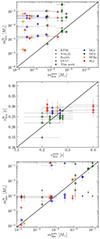 |
Fig. 1. Mass and velocity of the dynamical ejecta and disc mass from GW190425-targeted numerical simulations in Camilletti et al. (2022) ( |


In summary, we used Eqs. (6)–(8) to smoothly interpolate between fits calibrated in the two different regimes, corresponding to the PC and non-PC scenarios. Other BNS merger observations would be instrumental in improving these fits. In Figs. 2 and C.1 (in Appendix C), we display mdyn, vdyn, and mdisc, as defined in Eqs. (6)–(8), in the M1−M2 space for the BLh and APR4 EOS, respectively. BLh consistently predicts a larger disc mass than APR4 for fixed (M1, M2) values due to its lower compactness and greater tidal deformability. Comparing the amount of dynamically ejected mass predicted by the two EOSs is less immediate. If the merger remnant does not promptly collapse to a BH, then mdyn is dominated by the mass ejected at the remnant's rebounce, which is larger for more compact EOSs (Bauswein et al. 2013; Radice et al. 2018). In contrast, for prompt collapse scenarios, the dynamical ejecta comes primarily from the tidal matter tails formed before the coalescence, leading to less compact EOSs with larger tidal deformability ejecting more mass (e.g. Bernuzzi et al. 2020). The distinction between these two regimes is marked by the prompt collapse mass threshold, which also varies with the EOS, being smaller for more compact EOSs. Therefore, given the binary masses, APR4 predicts a larger mdyn than BLh only if the total binary mass is below the prompt-collapse mass threshold for APR4, as illustrated by comparing Figs. 2 and C.1.
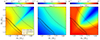 |
Fig. 2. Mass of the dynamical ejecta (left), velocity of the dynamical ejecta (centre), and mass of the disc (right) for the EOS BLh, as defined in Eqs. (6)–(8). x and y axes represent the masses M1 and M2 of the BNS. The solid and the dashed black lines mark the chirp mass of GW170817 and GW190425, respectively. Triangular markers show the prompt-collapse mass threshold MPC. |
We now detail the computation of mass, velocity, opacity, and angular distribution for the two ejecta components, C1 (anisotropic, including both the dynamical ejecta and ejecta unbound from the disc via spiral wave winds) and C2 (isotropic, accounting for the secular ejecta unbound from the disc on secular timescales), which were the input of the xkn KN model. We modelled the amount of mass in C1 as:
 (12)
(12)
where mdyn, defined in Eq. (6), represents the mass ejected dynamically, and msw denotes the mass ejected through spiral wave winds. Spiral wave winds are generated by NS remnants before the collapse to BH. Therefore, we set msw = 0 if Mtot≥MPC; otherwise, msw = 0.15 mdisc, where mdisc is defined in Eq. (8) and we assumed that spiral wave winds acting on timescales of several tens of ms are effective in unbind a significant fraction of the disc (Radice & Bernuzzi 2023). We distributed mC1 as F(θ) = sin(θ), where θ is the polar angle (cf. Perego et al. 2017; Radice et al. 2018). In general, matter ejected on a dynamical timescale and through spiral wave wind have different velocities. Hence, we define the central velocity of the first component as a weighted average:
 (13)
(13)
with vdyn from Eq. (7) and vsw = 0.17c (cf. Figure 2 in Nedora et al. 2019). The opacity for dynamical or spiral wave wind ejecta, kC1, varies with the polar angle. In general, the opacity is ∼10−20 cm2 g−1 in the equatorial region, while it is expected to reduce to ∼0.5−5 cm2 g−1 close to the poles, if strong enough shocks develop at the merger contact interface and if the merger remnant lives long enough to irradiate the polar ejecta with neutrinos (e.g. Kasen et al. 2013; Perego et al. 2014, 2017; Metzger & Fernández 2014; Martin et al. 2015; Sekiguchi et al. 2016). For asymmetric binaries (q≲0.7−0.75), the lighter NS is largely destroyed during the inspiral phase. Moreover, asymmetric binaries have a smaller prompt collapse mass threshold. Therefore, we applied the following prescription:
-
If
 , then we set kC1 = 1 cm2 g−1 in the polar region, θ≤50 deg and θ≥130 deg, and kC1 = 15 cm2 g−1 in the equatorial region, 50<θ<130 deg.
 -
If
 , then we set kC1 = 15 cm2 g−1 at all latitudes.
We assigned an entropy of sC1 = 10 kB/baryon and an ejecta expansion timescale τC1 = 5 ms for C1 (Radice et al. 2018).
We modelled the amount of mass in the second component as
 (14)
(14)
where mdisc is defined in Eq. (8) (c.f. the estimated amount of mass from AT2017gfo fitting in Perego et al. 2017). We assumed a uniformly distributed mass density and set the central velocity to vC2 = 0.06c. We assumed the opacity to be uniformly distributed and we set kC2 = 10 cm2 g−1. Finally, we set the entropy to sC2 = 20 kB/baryon, and the ejecta expansion timescale to τC2 = 33 ms (see e.g. Wu et al. 2016; Villar 2017; Perego et al. 2017).
In Figs. 3 and C.2 (in Appendix C), we show the ejecta component masses mC1 and mC2 in the M1−M2 space for BLh and APR4 EOSs, respectively. We notice that mC1 and mC2 are always larger for BLh than APR4, implying in general brighter KN light curves for BLh compared to APR4.
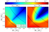 |
Fig. 3. Mass of the first component (left) and the second component (right) of the ejecta, as defined in Eqs. (12) and (14), respectively, for the EOS BLh. The solid and the dashed black lines mark the chirp mass of GW170817 and GW190425, respectively. |
2.4.2. Kilonova light curves
We computed the KN light curves for the previously described ejecta components using the xkn framework, a semi-analytic model designed for predicting and interpreting both the bolometric luminosity and broadband light curves of KNe (Ricigliano et al. 2024). This tool is particularly effective for extensive parameter estimation and population studies since it is computationally extremely efficient. Specifically, we adopted the xkn-diff model, which relies on a semi-analytical solution of the radiative transfer equation for homologously expanding material, in line with approaches developed in Pinto & Eastman (2000) and in the appendix of Wollaeger et al. (2018). The xkn-diff model simultaneously accounts for emission from both optically thick and thin ejecta, marking a significant advancement over previous semi-analytic methods. It also incorporates cosmological and K-corrections (Ricigliano et al. 2024).
For modelling the recombination effects in both lanthanide-free and lanthanide-rich ejecta, we established two floor temperatures: TNi = 3000 K and TLa = 1500 K (see Kasen et al. 2017; Kasen & Barnes 2019; Villar 2017; Breschi et al. 2021). Given the current uncertainties on the heating rate (e.g. Mendoza-Temis 2015; Rosswog et al. 2017; Zhu et al. 2021), stemming from variances in the nuclear mass model, we multiplied the nuclear heating rate,  , computed as per Ricigliano et al. (2024) using the FRDM nuclear mass model (Möller et al. 2016), by a factor
  . Its value was determined by ensuring the reproduction of the AT2017gfo case within our ejecta and KN light curve modelling (see Appendix C.1). For our two different EOS models, we find
  for BLh and
  for APR4. We notice that the heating rates
  resulting from these values are within their uncertainty range (Mendoza-Temis 2015; Rosswog et al. 2017; Zhu et al. 2021). In Appendix C.1, we test our choice, by comparing AT2017gfo to the KNe produced within our model for binaries with the same chirp mass as GW170817 and binary mass ratio q>0.725.
As discussed in Ricigliano et al. (2024), the simplified treatment of the opacity used in xkn introduces significant deviations in the KN light curves at early times after the merger, when compared to the results of radiative transfer calculations. For this reason, when using our light curves to develop an observational strategy with Rubin, we considered the computed emission to be reliable only starting from 1.5 hours after the merger.
2.5. Kilonova light curves distribution and properties
In this section, we examine the typical magnitude range of our KN light curve populations, focusing on KNe associated with BNS mergers detectable by ET-triangle. We select sources with a sky localisation uncertainty smaller than 100 deg2, which are suitable to be followed up with wide field-of-view optical telescopes, such as the Vera Rubin Observatory.
Fig. 4 presents the KN light curves and their probability distributions in the g and i filters of Rubin. These light curves are calculated for the BNS mergers detected by ET-triangle within 100 deg2 from populations characterised by a common envelope efficiency α = 1.0, Gaussian NS mass distribution, and BLh (left) and APR4 (right) EOSs. In the case of BLh EOS, the peak apparent AB magnitude for 90% of the KN distribution ranges between 26 mag and 21 mag in both filters. However, there's a noticeable variation in the peak times. For the 90% distribution range, this spans approximately between 5 and 12 hours for the g filter and between 9 and 24 hours for the i filter. For both g and i, the broad time range of the peak can be attributed to the differences in redshift among the light curves and time dilation in the observer frame. The delay observed going from redder to bluer emission is instead mainly due to the different opacities of the ejecta components. Of particular interest are two exceptionally bright light curves, with one reaching a magnitude of about 13 mag in the g filter, and the other around 18 mag. These correspond to relatively nearby and rare events, occurring at about 10 and 40 Mpc, respectively. These findings are slightly different for the APR4 EOS, where the light curves generally appear fainter by half to one magnitude and evolve more rapidly. This difference is attributed to the BLh EOS producing more massive ejecta in both components, C1 (dynamical and spiral wave wind ejecta) and C2 (secular ejecta), than APR4. This is evident when comparing Figs. 3 and C.2 within the mass range of [1.1, 1.6] M⊙ for both M1 and M2. Having a smaller mass threshold for prompt collapse and predicting smaller ejecta, the APR4 EOS consistently exhibits more light curves with a very rapid decay compared to BLh.
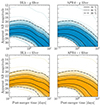 |
Fig. 4. KN light curves for the g (top) and i (bottom) filters. These light curves were generated from BNS merger fiducial populations, Gaussian NS mass distribution, and the BLh (left) and APR4 (right) EOSs. The plotted light curves are associated with BNS mergers detectable by ET reference design with a sky localisation accuracy better than 100 deg2. The solid, dashed, and dash-dot black lines mark the 50%, 90%, and 99% probability distributions of the light curves. |
The distribution properties of the light curves exhibit more pronounced variations in the case of uniform NS mass distribution, as illustrated in Fig. C.3 for the BLh (left) and APR4 (right) EOSs, respectively. While the peak magnitude range is similar to that of the Gaussian counterparts, with the light curves generally appearing slightly fainter, there is a notable spread in both the peak time and the duration of the light curve fading. The uniform mass distribution allows us to explore parts of the M1−M2 parameter space which are not accessible with Gaussian distributions. Specifically, systems with high chirp mass and near-unity mass ratios (visible in the upper right corners of Fig. 3 and Fig. C.2) have minimal ejecta, resulting in extremely faint KNe. Conversely, binaries with high chirp masses and highly asymmetric mass ratios (q≲0.7, as seen in the upper left and lower right corners of Fig. 3 and Fig. C.2) produce a small amount of ejecta (below 10−3 M⊙) in the first component, while the second ejecta component, originating from the tidally disrupted disc, is significantly more massive (exceeding 0.02 M⊙). These conditions lead to brighter KNe, particularly with the APR4 EOS. This is because, although the ejected mass is comparable for both EOSs, the larger nuclear factor  adopted for APR4 (necessary to reproduce AT2017gfo) results in brighter light curves. A comparison between our modelling of the KN light curves and AT2017gfo is provided in Appendix C and Figures C.4–C.5.
Finally, we compare our modelling of KN light curves with studies of short GRBs observed on-axis (some of them showing possible KN signatures in the afterglow emission) which evaluated the luminosity range for the KN emission (Ascenzi et al. 2019). To compare our results with the findings reported by Ascenzi et al. (2019), we computed the AB absolute magnitudes of the KN light curves presented in Fig. 5. For the BLh EOS, the peak magnitudes in the g filter span from –13.9 mag to –16.6 mag, with the peak occurring between 1.1 and 10.2 hours. Similarly, the APR4 EOS shows a peak magnitude range from –14.2 mag to –16.5 mag, occurring between 1 hour and 10.2 hours. Remarkably, our modelling aligns with the results of Ascenzi et al. (2019), who reports a peaking magnitude range of [–12.3, –16.8] mag in the g filter, occurring within 18 hours after the GRB prompt emission.
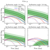 |
Fig. 5. GRB afterglow distribution (green region) compared to KNe light curves for BLh (blue lines) and APR4 (red lines) EOSs computed in the g filter of Rubin and at different inclination angles, assuming luminosity distance dL = 100 Mpc. The green line, dark green region and light green region correspond to the median, the 16–84 percentiles, and the 2.5–97.5 percentiles of the afterglow distribution, respectively. The KNe light curves correspond to three different BNS systems sampled from the BNS population with α = 1.0 and Gaussian mass distribution. Solid lines correspond to M1=M2 = 1.33 M⊙, that is the peak of the NS mass distribution; dashed lines correspond to M1 = 1.18 M⊙, M2 = 1.10 M⊙, that is the BNS producing the most massive disc; dotted lines correspond to M1=M2 = 1.57 M⊙, that is the BNS producing the lightest disc. |
2.6. Short GRB afterglow modelling
In addition to the emission due to the KNe, we included the contribution of the optical afterglows associated with the production of relativistic jets. One of the still uncertain parameters is the fraction fj of BNS mergers capable of successfully producing a jet. As detailed in Ronchini et al. (2022), the quantity fj can be deduced starting from a BNS merger population, knowing the local rate and its redshift evolution, and a phenomenological model of GRB prompt emission. Adopting a structured jet with an opening angle of 3.4° and an off-core power-law profile with a slope s = 4, Ronchini et al. (2022) obtain a median value fj = 0.26. However, fj must be adjusted accordingly for different BNS population synthesis tracks to maintain the same local short GRB rate. Therefore, denoting with a tilde the quantities adopted in Ronchini et al. (2022), we computed
 (15)
(15)
For our BNS population with α = 1.0, we obtain an fj value of 0.7, and for α = 0.5, fj reaches 1.0.
To evaluate the afterglow emission, we used the Python package afterglowpy (Ryan et al. 2020). The jet structure followed the functional form derived in Ghirlanda et al. (2019). The isotropic-equivalent kinetic energy of the jet was derived starting from the isotropic prompt energy extracted from the posterior distribution in Ronchini et al. (2022). Adjusted for the jet's aperture angle, the distribution of the jet kinetic energy is compatible with the one reported in Fong et al. (2015). Our micro-physical parameters include ϵe = 0.1, p = 2.2, log10ϵB uniformly distributed in the range [−4, −2], and n∈[0.25, 15]×10−3 cm−3. These parameters allowed us to replicate the observed range of short GRB afterglow luminosities in optical and X-ray bands, as documented in Kann et al. (2011) and Fong et al. (2015).
Figures 5 and 6 compare jet afterglows and the KN emissions for APR4 (red lines) and BLh (blue lines) in g and i filters at 100 Mpc luminosity distance, considering different inclination angles. We display the median and percentiles (2.5, 16, 84, and 97.5) of afterglow distributions and three relevant cases of KN emissions:
-
average KNe (solid lines): we consider an equal mass BNS with masses corresponding to the peak of the Gaussian distribution, that is M1=M2 = 1.33 M⊙;
-
very bright KNe (dashed lines): we select the BNS producing the disc with the largest mass (M1 = 1.18 M⊙, M2 = 1.10 M⊙) from the BNS population with α = 1.0 and Gaussian mass distribution and compute the corresponding KN;
-
very faint KNe (dotted lines): we select the BNS producing the disc with the smallest mass (M1=M2 = 1.57 M⊙) from the BNS population with α = 1.0 and Gaussian mass distribution and compute the corresponding KN.
Jet afterglows outshine the faintest KNe in the entire time domain for inclination angles ι<15−20 deg. In contrast, KNe dominate early emissions at ι≥20 deg, as expected. The brightest KNe overcome a non-negligible portion of the afterglow emission distribution at any angle a few hours after the merger. The behaviour of the average KNe strongly depends on the nuclear EOS. In particular, the peak of the KN computed assuming the BLh EOS is on average significantly brighter than the one corresponding to the APR4 EOS. Accordingly, the probability of observing the peak of the KN emission above the afterglow emission at ι∼5−10 deg is enhanced for the BLh EOS.
We simulated our observational strategy with Rubin by considering (1) only the KN emission and (2) the sum of the KN emission and the afterglow emission from the jet.
3. Rubin observational strategy
This section outlines our observational strategy with the Rubin Observatory (Ivezić et al. 2019) to detect the optical counterparts of GW signals. Rubin is a large and wide field-of-view (9.6 deg2) ground-based telescope, comprising an 8.4 m primary mirror and a 3.2 gigapixel camera combined in a stiff compact design enabling an extremely fast slewing time. It is currently the most innovative observatory providing capabilities for rapidly covering large sky regions (through a mosaic strategy) reaching deep sensitivity with short exposures in several filters. This makes it the optimal instrument for observing the relatively faint KN counterparts of BNS mergers detected by next-generation GW detectors.
We propose to use ToO observations as the most effective follow-up strategy. This enables us to rapidly point to the sky-localisation associated with GW signal, to use the appropriate exposure time and to repeat the observation with the right cadence for KN detection. Considering that the next generation of GW observatories is expected to be operative after 2035 when Rubin is planned to have completed its decadal surveys and achieved its associated objectives, we assumed the availability of a large amount of observational time for ToO programs.
We designed an observational strategy based on following up all the events with a sky-localisation uncertainty (given as 90% credible region) below a certain threshold value. This choice makes it possible to maximize the number of events to follow while keeping Rubin's time within a reasonable amount. We considered only events within the sky regions accessible to Rubin8. This made our simulations account for the combination of the real sky-direction sensitivity of the GW network and the Rubin-accessible sky.
We adopted a multi-filter and multi-epoch observational strategy. This strategy enabled us to have indications of the source spectra and colour evolution, which is particularly important to identify the candidate counterparts and remove contaminant events. Multi-filter observations were scheduled in two epochs over 2 or 3 nights, starting from the first night after the merger. We took sunrise and sunset times into account and started the follow-up as soon as it was feasible after sunset. Given the merger time tc, we started the observations as soon as possible, but never earlier than tc+1.5 hours after the merger, because our KN modelling is less reliable at very early times. Sunrise and sunset times were taken to be 6:30 am and 7:30 pm, allowing for 11 hours of darkness per night, which is an average for Cerro Pachon throughout the seasons9. We used the g and i filters. The i filter is preferred over z for this study since it allows for deeper point-source photometry in a single exposure while it is still expected to enable contaminant removal following the g−i colour evolution (Cowperthwaite et al. 2019; Andreoni et al. 2019; Bianco et al. 2019). For each epoch, the observations were performed starting with the g filter, completing the mosaic, and then switching to the i filter and observing the mosaic again. If the mosaic was completed in one night in the first epoch, the second epoch started after the next sunset. If the mosaic could not be completed during the first night, observations of the first epoch were resumed from the point where they were interrupted immediately after the next sunset. Thus, the first and second epoch observations were performed during the two or three consecutive nights after the merger. We used single exposures of 600 s for each pointing, but we also tested strategies which make use of deeper exposures of 1200 s (see Sect. 4.4). The overhead for filter change and the slewing time to cover the mosaic in each filter was considered to be 220 s for each epoch10. This time takes into account that Rubin's mirrors have the ability to slew extremely fast with a median slew time of ∼5 s (Bianco et al. 2021) and that the filter change time is of the order of two minutes if the filter is already mounted on the wheel (five out of the six filters will be housed on the wheel at all times).
The total Rubin follow-up time to observe all the selected GW events was determined as:
 (16)
(16)
where N(<Ω90, max) is the number of events detected by a GW network with sky localisation smaller than Ω90, max in the Rubin footprint, and tobs, i is the Rubin observational time spent to tile the whole localisation area for each of these events in two filters and two epochs. For each event, this time was given by
 (17)
(17)
where npointings, i is the total number of pointings of the mosaic obtained by dividing the sky-localisation uncertainty of each event for the Rubin field of view as
 (18)
(18)
texp is the exposure time (in seconds) for each pointing, nfilters = 2 is the number of filters, and nepochs = 2 is the number of epochs. The tobs, i estimate includes 440 s (about seven minutes) of overhead for the mosaic slewing time and for changing filters as detailed above.
Andreoni et al. (2022b) propose using more than two filters and shorter exposure times as an effective strategy to follow GW events detected by current GW detectors. In contrast, our two-filter strategy seeks to minimise the observational resources required for a single event in order to maximise the number of events to be followed. This is important to make the most of the larger number of events detected by next-generation GW observatories compared to the current ones. Here, we favour longer exposures to reach a larger distance and therefore to detect weaker KNe. Additionally, we use g and i filters since they are capable of capturing the unique features that can distinguish the evolution of a KN from other transients.
The criteria for detection were set based on the 5σ depth for a single exposure of 600 s (or of 1200 s), calculated at a conservative airmass at 45deg from zenith11. Specifically, for the g band, the 5σ depth is 26.53 mag at 600 s exposure and 26.91 mag at 1200 s in units of ABmag. In the case of the i band, 5σ depth is 25.59 mag at 600 s exposure and 25.97 mag at 1200 s. For each detected GW event, we computed the total number of pointings needed to cover its sky localisation (90% credible region) and we randomly assigned a position to the GW source in one of these mosaic tiles, assuming a uniform distribution within the localization area12. We then evaluated the flux at the time when the observation arrived at the tile containing the source and determined if it was brighter than the 5σ threshold. We highlight that numbers and plots referring to the joint detections provided in Sect. 4.2 were obtained by injecting and recovering the signals within the targeted 90% credible region, thus, the readers should take into account a 10% reduction for sources located outside the targeted region.
Our light curves were pre-processed to take into account the effect of Galactic absorption. We included the extinction correction for each filter obtained from Green (2018), based on Schlegel et al. (1998) and Schlafly & Finkbeiner (2011), considering the precise sky location of each BNS merger.
We considered two detection strategies, designated as one epoch detection (1ep), and two epoch detection (2ep). The 1ep strategy requires the optical counterpart to be detected at least once in both filters during the same epoch observations. The 2ep criterion is more conservative and requires the source to be detected in the two filters in the first epoch and at least in the i filter in the second epoch (the KN is typically expected to show a slower decline in the redder filter compared to the bluer one). The 2ep events are a subset of the ones detected following the 1ep criterion, but multiple detections in the first and second epoch enable us to follow the colour evolution in the first days which can be crucial to distinguish the optical counterpart of GW event among many contaminants. In Table 3, we list the requirements to classify an event as detected according to the 1ep and 2ep strategies.
Truth table of our observational strategy with Rubin, using filters g and i.
This work focuses on KN detection based on photometric data. However, all the modelling and simulations developed for the present work have been used to explore KN spectroscopy (Bisero et al., in prep.) and in particular to investigate the multi-messenger science case for the WST project (Mainieri et al. 2024). WST is a proposed innovative 12-m class spectroscopic telescope with simultaneous operation of a large field-of-view (3 deg2) and a high multiplex (20 000) multi-object spectrograph facility.
4. Results and discussion
4.1. GW detection and parameter estimation forecasting
This section summarises and discusses the outcomes of the 64 simulations described in Sect. 2.3, focusing on the detection capabilities and the associated parameter estimation of the considered GW detectors.
Fig. 7 shows the number of detections over ten years up to redshift z = 1 for the fiducial population (α = 1), assuming a uniform NS mass distribution and the BLh EOS. As found in Branchesi et al. (2023), the 2L ET performs better than the ET-triangle; the total number of detections up to z = 1 increases by about 30%. The detection capabilities of both the 2L and triangle configurations of ET are enhanced when operating within a network of detectors. In particular, the number of detections increases by about 3% when ET operates with current detectors (LVKI O5 sensitivities). The number of detections increases by approximately 70% (90%) when ET-triangle is part of a network with next-generation detectors, including one CE (two CEs). For ET-2L, the number of detections increases by about 30% (40%). In Appendix D, we detail the absolute number of detections for the different EOSs and NS mass distributions analysed in the present paper. In particular, Fig. D.1 shows the number of detections for the BLh EOS and Gaussian NS mass distribution, in parallel to Fig. 7.
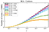 |
Fig. 7. Ten-year detection distribution as a function of redshift for the eight different networks using the fiducial population (α = 1) with BLh EOS and uniform mass distribution. |
Fig. 8 compares ET's triangle detection numbers up to z = 1 across different choices for the NS mass distribution and the EOS. For the uniform mass distribution, the number of detections increases by about 20–25% compared to the Gaussian mass distribution, regardless of the EOS. This is expected due to the larger masses achieved by binary systems with a uniform NS mass distribution. Comparing the EOSs the differences are negligible. We only observe that APR4 yields a slightly higher number of detections (by 3%) than BLh for the uniform mass distribution. This effect is mainly driven by the larger maximum NS mass supported by APR4, leading to louder GW signals. These findings agree with the analysis by Iacovelli et al. (2023), who observes an increased detection rate for EOSs with a higher maximum mass, specifically under a uniform NS mass distribution.
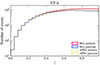 |
Fig. 8. Ten-year detection distribution as a function of redshift for the reference ET-triangle using the fiducial population (α = 1) and comparing different NS mass distributions and EOS models. |
The sky-localisation capabilities of ET, operating either alone or in a network of detectors, are summarised in Tables D.2 and D.3 for ET-triangle and 2L, respectively. These tables list the number of detections over ten years by various detector networks with sky-localisation accuracy, Ω90, smaller than certain thresholds in the case of the pessimistic population (α = 0.5) and the fiducial one (α = 1), for the analysed NS EOSs (APR4 and BLh) and NS mass distributions (uniform and Gaussian). The results obtained for α = 0.5 (top of the tables) and α = 1.0 (bottom of the tables) show the large uncertainties in the absolute detection numbers due to the difference in the common envelope efficiency. The fiducial population provides a factor five higher number of detections with sky localisation smaller than 100 deg2 compared to the pessimistic one. As previously underlined, this is consistent with the poor observational constraints on the local BNS merger rate.
Comparing Tables D.2 and D.3, we find that ET-2L operating as a single observatory localises better than ET-triangle by detecting a factor 2.4 more events within sky-localisation 100 deg2. This is also found for ET operating together with current detectors, where ET-2L allows for 40–50% more detections within 100 deg2 compared to ET-triangle. The better performances of ET-2L in source localisation are still visible when ET operates in a network with one CE; in this case, ET-2L localises better than 10 deg2 about 30–40% more events compared to ET-triangle. When ET is operating with two CEs, the difference between 2L and triangle is negligible, except for the events localised better than 1 deg2. These results are fully consistent with the findings of Branchesi et al. (2023) for ET alone and ET plus one CE in the USA.
The number of well-localised events dramatically increases when ET operates in a network of detectors, as shown in Tables D.2 and D.3. For the fiducial population, the number of events localised better than 100 deg2 increases from a few hundred per year to several thousand per year when ET operates with current detectors (LVKI) rather than alone. ET will significantly benefit from the presence of current detectors (mainly from the distant ones, while Virgo gives a negligible contribution due to its vicinity), and the number of events detected better than 10 deg2 will increase from a few tens to a few hundreds per year. Fig. 9 shows the benefits carried by detector networks in terms of larger redshifts reached by well-localised events. The presence of a network of next-generation detectors brings the number of events localised better than 10 deg2 to 103 (104) per year for ET+1CE (ET+2CE) up to z∼0.9−1.0.
 |
Fig. 9. Number of injected events and events localised better than 100 deg2, 40 deg2, 20 deg2, 10 deg2, and 1 deg2 by the different detector networks considered in this work for the fiducial population (α = 1) obtained assuming the BLh EOS and uniform NS mass distribution. The left plots show the ET-triangle and the right plots ET-2L shape. In Appendix D, we show the same plots for BLh Gaussian NS mass distribution, and APR4 uniform and Gaussian NS mass distribution. |
The larger number of GW detections for the uniform mass distribution compared to the Gaussian one results in a systematically larger number of well-localised events in the case of uniform mass distribution. Moreover, for a given luminosity distance, the accuracy of sky localisation tends to be higher in the uniform distribution scenario due to the presence of more massive systems, which generate higher SNRs.
Finally, also the NS EOS affects the number of GW detections at a given sky localisation. A comparison between the number of detected events for APR4 and BLh at Ω90<100, 40, 20, 10 deg2 shows that typically the number of detections increases for APR4 up to 4%, in the case of Gaussian mass distribution, and 10%, in the case of uniform mass distribution. This is because APR4 is more compact, therefore it has smaller tidal deformability compared to BLh (see Figs. A.1 and A.2), so the inspiral of the GW signal lasts more time in the detector. Moreover, as mentioned above, in the case of uniform mass distribution, APR4 supports a larger maximum NS mass with respect to BLh (see Table 1) providing systems with larger mass, and thus larger SNR which can improve the sky localisation.
Fig. 10 presents the SNR distributions for the injected signals and the parameter estimation for the detected sources (SNR > 8), highlighting the uncertainties in chirp mass, luminosity distance, inclination angle, and tidal deformabilities for the fiducial population (α = 1) with a uniform NS mass distribution and BLh EOS. Notably, the parameter estimation accuracy is significantly enhanced with the 2L ET compared to the triangular configuration when each operates as a single detector. This enhancement, albeit less significant, persists when ET is operating in a network of detectors. It is noteworthy to highlight the improved estimation of parameters already reached when ET operates in synergy with current detectors. This is particularly relevant for the estimate of the luminosity distance, which is the key parameter for cosmology studies. This finding is pertinent to the redshift range z = 0−1 considered in this study, as extending to higher redshifts the presence of current detectors would not improve parameter estimation. The parameter estimation accuracy further increases with the inclusion of next-generation detectors, as evidenced by the distribution of well-localised events as a function of redshift (see Fig. 9 and Figures in Appendix D).
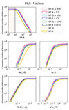 |
Fig. 10. Distribution of SNR and relative errors on detector frame chirp mass, ℳc, luminosity distance dL, inclination angle ι, and first component tidal deformability Λ1. These results are obtained for the fiducial population (α = 1.0) and assuming a uniform NS mass distribution with BLh EOS. |
In Appendix D, we show the SNR distributions and the relative uncertainties on chirp mass, luminosity distance, inclination angle, and tidal deformabilities for the fiducial population, but considering the Gaussian NS mass distribution with BLh and the uniform NS mass distribution with APR4. These plots show results consistent with those described above.
4.2. Joint GW and optical detections
The results of our simulations reproducing different scenarios of GW detectors including ET-triangle operating in synergy with Rubin are summarised in Figs. 11, E.1, and Table 4. Similarly, the results for the 2L ET are reported in Figures E.2–E.3 and Table E.1.
Number of joint detections by Rubin operating in synergy with ET triangular shape operating as a single observatory, and as part of a global network of GW detectors (indicated in the second column from the left).
Fig. 11 refers to the BLh EOS and shows: (1) the total observational time (see Eq. (16)) required to follow up all the GW events visible by Rubin with sky-localisation uncertainty within threshold Ω90, and (2) the corresponding joint (KN and KN+GRB) detection numbers. In other words, if the observer decides to follow up all the events within a certain sky localisation (Ω90, x-axis), the required Rubin time is indicated on the y-axis, while the joint detection number is shown on the y-axis of the corresponding right plot. The total time and number of detections are given for ten years of observations. The left panels show horizontal lines corresponding to the percentages (10%, 50%, 100%) of the Rubin's total observational time which is obtained by dividing the total observational time for the GW follow-up by the total 10-year observing time of Rubin. We assumed a total Rubin observational time of 3600 hours per year considering 11 hours of dark time each night in a year and a Rubin duty cycle of 90%. Each plot shows the results for the fiducial (thick lines) and pessimistic (thin lines) populations. All the panels refer to the 1ep strategy. In Appendix E, we provide the corresponding figures showing the results for the APR4 EOS and the 2L-shaped ET.
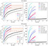 |
Fig. 11. Cumulative time required and total number of joint detections for Rubin follow up. Left panels: cumulative time necessary to follow up all the events in the Rubin footprint with a sky localisation smaller than Ω90 (indicated in the x-axis) for ET-triangle as a single observatory, and included in a network of current and future GW detectors as indicated in the legend. The horizontal dashed lines indicate the time corresponding to 10%, 50%, and 100% of Rubin's total observational time in 10 years. Right panels: the corresponding number of optical detections by Rubin. Solid lines are for the KN emission, while dashed lines are for the KN+GRB afterglow. All plots refer to the BLh EOS; the top row plots are obtained using the uniform NS mass distribution and the bottom row ones for the Gaussian NS mass distribution. Thick lines represent the fiducial population (α = 1.0) whereas the thin lines represent the pessimistic population (α = 0.5). |
Tables 4 and E.1 list the number of events followed and detected over ten years by Rubin operating in synergy with ET triangle-shaped and 2L-shaped, respectively. They show the results for ET alone and operating within the network of GW detectors, assuming for each event only KN emission or KN and GRB afterglow emission, and considering the two NS EOSs (APR4 and BLh), and the two NS mass distributions (uniform and Gaussian). The results are given for both the pessimistic (α = 0.5) and fiducial (α = 1.0) populations of BNS mergers, and considering the two detection strategies (1ep and 2ep) described in Sect. 3. Our selection criteria for the events to be followed up are determined by the sky-localisation accuracy achievable through GW signal analysis, which varies by detector network configuration. In Fig. 11, we provide readers with all the necessary information to define their own sky-localisation thresholds for selecting triggers while considering the time required for the follow-up. In contrast, Tables 4 and E.1, present specific thresholds to illustrate a feasible example of selection. In particular, we use Ω90<100 deg2 for ET alone (both triangular and 2L shapes), Ω90<20 deg2 when ET operates with current detectors, Ω90<10 deg2 for ET and one CE, and Ω90<5 deg2 for ET and two CEs. Our threshold choice wants to maximize the number of joint detections while keeping the Rubin time allocated for the GW follow-up reasonable (within 30% of the Rubin observational time). An exception is made for the ET+2CEs network with α = 1.0, since in this case the number of events localised better than 5 deg2 corresponds to several thousands per year and the time exceeds the total Rubin observational time. In Appendix E, Table E.2 shows the number of joint detections and corresponding Rubin's time allocation resulting from a narrower cut Ω90<1 deg2 on the sky localisation of the events detected by ET + 2CEs. Selecting the events within 1 deg2 reduces the required observational time while maintaining a high number of detections (about hundreds per year), similar to ET+1CE. However, in this case, also smaller field-of-view telescopes could be used instead of Rubin.
4.2.1. Joint detection efficiency
We evaluate the joint GW/optical detection efficiency as a function of redshift by dividing the number of joint detections by the number of followed-up events (namely, events detected by the GW detector network within a certain sky-localisation threshold and in the Rubin footprint) in increasing redshift bins of 0.05. The sky-localisation thresholds correspond to the maximum values of Ω90 used for Fig. 11, namely Ω90<100 deg2 for ET alone, Ω90<40 deg2 for ET+LVKI and for ET+1CE, and Ω90<20 deg2 for ET+2CEs. As an example, Fig. 12 shows the detection efficiency for the fiducial population (α = 1.0), the BLh EOS, the uniform NS mass distribution, and the 1ep strategy. The right panels of the same figure show the distribution of the inclination angle, ι, for the GW events detected within the aforementioned sky localisation thresholds (GW), the subset of these events within the Rubin footprint (fp), and the corresponding KN and the KN+GRB counterpart detections. Each row in the figure represents a different GW detector network, starting from the top with ET as a single observatory, ET+LVKI, ET+1CE, and ET+2CE. The same plots for the Gaussian NS mass distribution and APR4 EOS are given in Appendix E.
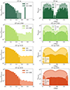 |
Fig. 12. Efficiency of joint detections and distribution of inclination angles of BNS mergers. Left panels: efficiency of joint detections as a function of redshift for ET-Δ in each network configuration for both KN (hashed) and KN+GRB (solid) histograms. Right panels: distribution of the inclination angle, ι, for each network configuration indicated in the legends of the left panels. The plots show all the detected (GW) events with a sky localisation within Ω90<100 deg2 for ET alone, Ω90<40 deg2 for ET+LVKI and ET+1CE, and Ω90<20 deg2 for ET+2CE (as used for Fig. 11), the events followed-up as within the Rubin footprint (fp), the corresponding KN detections, and the KN+GRB detections. The plots show the results obtained for the BLh EoS and the uniform NS mass distribution using the 1ep strategy. |
Focusing on the inclination angle plots (right panels of Fig. 12), the distribution of ι for the joint detections closely resembles that of the sources detected in GWs displaying fewer events for face-on systems (ι around 0 and 180 deg). This is fully consistent with the expectations for a population of randomly oriented systems in a sphere leading to fewer observable face-on systems than edge-on ones. There is also a lower density of GW detections around the region of the edge-on systems (ι = 90 deg). This under-density is due to the SNR being lower for edge-on systems than for face-on ones with the same intrinsic parameters. Lower SNR values cause a smaller ratio of detected to injected signals for edge-on systems and the worsening of sky localisation.
Focusing on the GW/KN detection efficiency plots, we note that the efficiency drops to 50% already at redshift ∼0.25−0.3. Fig. 9 shows that the GW events selected for the follow-up based on sky-localisation thresholds extend to much higher redshifts. Thus, this reduction in efficiency at relatively low redshifts is due to the limited detection capability of the Rubin observations whose sensitivity is not enough to detect KN emission at larger redshifts. Adding the GRB afterglow emission from the relativistic jet, a tail of detections at higher redshifts appears (KN+GRB case). Indeed, the distribution of the ι for the KN+GRB detections shows that the overdensity of events largely comes from BNS systems with low inclination angles (on-axis and also some off-axis events, 0<ι<15 deg or 165 deg<ι<180 deg). When the BNS merger is able to produce a jet and the system is oriented almost on-axis, the beamed GRB afterglow emission which is typically brighter than the KN emission enables us to detect the optical counterparts at higher redshifts. This is also aided by the fact that the GW signal of on-axis events is louder compared to the off-axis ones leading to on-axis events being well-localised even at higher z.
It is noteworthy that the efficiency never quite reaches 100%, implying that not all KNe are detected even when the sources are at low redshifts. This is due to a combination of multiple factors, the first of which is the fact that we have considered realistic extinction correction for each merger based on their location on-sky. The large absorption for sources in the Galactic plane causes the light curves to become fainter than the Rubin detection limit. Analyzing sources within z = 0.1 (where we can limit the effect of distance making the source fainter) high extinction events make up 2–7% of the events followed up by Rubin but account for 100% of events not detected for ET-triangle and ET-2L for all the networks in the case of the NS Gaussian mass distribution, for both BLh and APR4 EOS. For the NS uniform mass distribution, high extinction events make up 40–75% (40–60%) of the events not detected for the BLh (APR4) EOS. While the Gaussian mass distribution produces brighter light curves, and the only events not detected at low redshifts are due to high extinction close to the Galactic plane, the NS uniform mass distribution produces fainter light curves that cannot be detected by Rubin due to their intrinsic properties and not necessarily due to higher galactic extinction. Since BLh produces slightly brighter light curves than APR4, the percentage of events not detected due to being intrinsically faint is slightly lower for the case of BLh than for APR4.
4.2.2. Network comparison: joint detection numbers versus observational time
The right panels of Fig. 11 show that by setting a threshold on the sky localisation of events to be followed up by Rubin, a large increase in detections can potentially be achieved with networks of GW detectors. For example, selecting a threshold of 20 deg2, ET operating together with the network of current detectors (LVKI) enables us to detect an order of magnitude more events than ET operating as a single observatory. The joint GW/KN detection number further increases by a factor of two if ET operates together with one CE. On the other hand, taking as reference the fiducial population with uniform BNS mass distribution and the BLh EOS (see Fig. 11), if we set a threshold on the observational time allocated for GW follow-up to a value equal to 10% (50%) of Rubin's time, this corresponds to the sky location thresholds of 15 deg2 (30 deg2) and 5 deg2 (15 deg2) for ET+LVKI and ET+1CE, respectively. This selection results in ET+1CE detecting about 30% (40%) more KNe than ET+LVKI. These results show that while the GW detections within similar sky-localisation thresholds significantly increase (by about a factor of 5), we have a much lower increase in KNe detection. The detection efficiency of KNe with ET operating with new-generation detectors (CE) is not much better than that obtained with ET+LVKI. This is largely due to Rubin's detection efficiency being limited to relatively small redshifts (see Sect. 4.2.1), where the network of current detectors is sensitive, and the large baselines created by distant detectors would already enable optimal sky-localisation capability with ET. In the scenario of ET+CE, there is a much larger number of GW triggers relatively well-localised to be followed up, and among them, a larger fraction is expected to not have a detectable optical counterpart due to the source being too distant and faint. In the case of ET in a network with next-generation detectors, it will be necessary to develop a more careful prioritization of the events to be followed up, which must be tailored for specific science goals and eventually increase the exposure time of each pointing. Such a prioritization would need to make use of other source parameters to identify the events to be followed (e.g. the distance and/or SNR).
4.2.3. ET-triangle versus 2L
Here, we compare the KN detection performance of Rubin operating with ET-triangle versus ET-2L, either as a single observatory or within a network of GW detectors. As a reference example, we focus on the 1ep detection strategy with Rubin, the fiducial population, the BLh EOS, and the uniform NS mass distribution. Our findings reveal that the 2L configuration of ET significantly outperforms the triangular one in terms of KN detection capability when ET operates as a single observatory; the 2L-shaped configuration detects a factor of 2.2 more KNe compared to the triangular one. However, this increase is reduced to 20% when ET operates in a network with LVKI and becomes negligible when ET operates together with one or two CEs. Similar results are obtained by varying the NS mass distribution and EOS. The observed difference in KN joint detection rates between ET-triangle and ET-2L for ET operating as a single observatory is closely linked to their source localisation capabilities. As discussed in Sect. 4.1, the ET-2L has a superior ability to localise sources within an area smaller than 100 deg2, identifying 2.4 times more sources than the ET-triangle. The reduced difference in the joint KN detection rates between the ET-triangle and the ET-2L when operating in a network of GW detectors is because localisation is provided by the much wider baseline provided by distant detectors of the network which allows for better triangulation based on the signal arrival time. Adding the GRB optical afterglow to the KN emission, we find that ET-2L outperforms ET-triangle, exhibiting the same percentual increase in the number of detections already observed for KN-only emission.
4.2.4. KN detections by Rubin
Impact of the BNS populations
The analysis of KN detection numbers with α = 0.5 and α = 1.0, as detailed in Tables 4 and E.1, reveals that α = 1.0 yields approximately a factor of 5 more detections across all configurations of GW networks, NS EOSs (APR4 and BLh), and NS mass distributions (uniform and Gaussian). The same increase is found in the number of events located within a certain threshold, as reported in Tables D.2 and D.3. Such findings are consistent with the different normalization in the local counts of BNS mergers for the two populations considered in this work.
This uncertainty is within the range of astrophysical BNS merger rates derived from the first three observation runs of LIGO and Virgo (10–1700 Gpc−3 yr−1) (Abbott et al. 2023). Our fiducial population is consistent with the fourth run of LVK observations, which has been ongoing for more than a year without any BNS detection, disfavouring the most optimistic merger rate.
Impact of NS EOSs and NS mass distributions
We explore the influence of the KN modelling on the detection rates of KNe by Rubin using the 1ep observational strategy. We focus on the results obtained with the fiducial population. To provide a clear analysis, we organise the comparison by holding either the NS mass distribution or the EOS constant.
When the mass distribution is Gaussian, the detection rates of KNe favour the BLh EOS over APR4. Specifically, the BLh EOS results in 20% more detections for ET operating as a single observatory. This advantage increases for ET in a network, yielding 30% more detections with ET+LVKI, 40% more detections with ET+1CE, and 60% more detections with ET+2CEs, regardless of the ET's geometry. Conversely, when the mass distribution is uniform, the APR4 EOS leads to higher KNe detection rates than BLh; by less than 10% for an ET operating alone and approximately 20% for ET in networks, consistently across different ET geometries.
With the APR4 EOS, uniform mass distributions are generally associated with higher KNe detection rates than Gaussian distributions, with the difference around 10% across all networks13. For the BLh EOS, Gaussian mass distributions significantly outperform uniform distributions in KNe detections, with differences ranging between 40% to 70%, depending on the network configuration.
To understand these trends, we analyse and compare the number of well-localised GW events and corresponding KN detections in the space defined by the binary masses M1 and M2. Figs. 13 and 14 display the number of GW detections localised by ET-triangle+2CEs within Ω90<5 deg2 and the corresponding KN detections, considering Gaussian and uniform mass distributions, respectively, for both APR4 and BLh EOSs. In the case of Gaussian NS mass distribution, NS masses span from 1.1 M⊙ to approximately 1.7 M⊙, maintaining an identical component mass distribution for both the EOSs under consideration (also refer to Fig. A.1). This reflects on the distribution of GW well-localised events in the M1−M2 space, which does not depend on the EOS, consistently peaking near the peak of the Gaussian mass distribution M1, 2 = 1.33 M⊙, as shown in the left plots of Fig. 13. Conversely, the distribution of KNe detections within the M1−M2 plane exhibits a pronounced EOS dependence. For both the EOSs, the KN detections lie in the region corresponding to binaries with total mass below the prompt collapse mass threshold (lower left quadrant). However, the BLh presents a peak around M1, 2≃1.33 M⊙, which is instead suppressed in the case of APR4 EOS, and more KN detections across the entire M1−M2 space. Using the Gaussian mass distribution, we explore a portion of the M1−M2 space where BLh EOS predicts ejecta masses, mC1 and mC2, largely exceeding those predicted by APR4, as shown by comparing Figs. 3 and C.2. Therefore, BLh generates brighter KNe enhancing their detectability by Rubin.
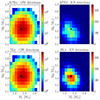 |
Fig. 13. Number of GW and KN detections in the M1−M2 space. The colorbar indicates the number of GW detections with sky localisation Ω90<5 deg2 (left) and the number of corresponding KN detections for the 1ep detection strategy (right) obtained assuming APR4 (top) and BLh (bottom) EOSs, Gaussian NS mass distribution, α = 1.0, and GW network ET-Δ+2 CE. The black dot shows the peak of the Gaussian mass distribution, that is M1=M2 = 1.33 M⊙. |
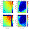 |
Fig. 14. Same as Fig. 13 but for the uniform NS mass distribution. The black dot shows the peak of the Gaussian mass distribution, that is M1=M2 = 1.33 M⊙. |
Unlike the Gaussian distribution, the uniform mass distribution scenario shows a distinct EOS-dependent variation in the distribution of well-localised GW events within the M1−M2 space (see Fig. 14). Although in the case of uniform NS mass distribution there is a trend of having more well-localised GW events with the APR4 EOS compared to BLh reaching up to a 10% increase, as detailed in Sect. 4.1, Fig. 14 illustrates how for binaries with component masses M1, 2≤2.1 M⊙ the BLh EOS is associated with a higher rate of GW detections per mass bin compared to APR4. This discrepancy arises because all mergers of the population (injected events) are spread across a broader M1−M2 space for APR4 than for BLh since APR4 accommodates a larger maximum NS mass (see Table 1). To better understand the pattern observed in KNe detections, it is instructive to divide the binary mass space (M1−M2) into three distinct regions, each characterised by a different distribution of KNe detections. These regions are delineated based on the masses of the BNSs and their mass ratios (q):
-
low-mass binaries, including binaries with individual masses ranging from 1.1 M⊙ to 1.6 M⊙ (lower left corner of KN detections plots in Fig. 14). The total mass of the majority of these binaries is below the prompt collapse mass threshold.
-
high-mass and symmetric binaries, including binaries with individual masses ranging approximately from 1.6 M⊙ to 2.20 M⊙, with mass ratios close to unity q∼0.8−1.0 (upper right corner of KN detections plots in Fig. 14).
-
highly asymmetric binaries, including binaries where one NS is significantly heavier than its companion, with masses for the heavier component in the 1.6 M⊙−Mmax range and the lighter one in the 1.1−1.6 M⊙ range, resulting in mass ratios q∼0.5−0.7. The total mass of the majority of these systems surpasses the prompt collapse mass threshold.
Fig. 14, specifically the plots on the right, reveals that BLh yields a larger number of KNe detections compared to APR4 within the low-mass binary region. This outcome aligns with expectations, as this portion of the M1−M2 space is characterised by a significantly higher ejected mass for BLh than for APR4 (see Figs. 3 and C.2), in analogy with the case of Gaussian mass distribution. The region of the M1−M2 space populated by high-mass and symmetric binaries, instead, is characterised by a minimal amount of ejected mass across both the EOSs, leading to uniformly dimmer KNe. This outcome results in KNe emissions that frequently fall beneath Rubin's sensitivity threshold, as set in our strategy, and are not detected. Finally, in the region of highly asymmetric binaries, the dominant contribution to the ejected mass comes from material unbound from the accretion disc. Interestingly, the amount of ejected mass is relatively similar for both the APR4 and BLh EOSs, as depicted in Figures 3 and C.2 and discussed in Sect. 2.4.1. Within our modelling, when the ejected masses are comparable across different EOSs, the differences in the brightness and temporal evolution of the KN emission become primarily influenced by the choice of nuclear factor,  , which multiplies the nuclear heating rate. Notably, in order to correctly reproduce AT2017gfo, we associate APR4 with a higher value of
  . Given that the ejected mass and its velocity remain essentially the same across both EOSs, the APR4 EOS leads to KNe which are not only brighter but also exhibit a slower fading pattern in their light curves. According to our analysis, approximately 20% of the well-localised binaries fall within the low-mass binary region, where BLh results in brighter KNe. Conversely, about 50% of the well-localised binaries are situated in the highly asymmetric binary region, which favours APR4 in terms of producing brighter KNe. Therefore, the total count of KNe detections is higher for the APR4 EOS.
This analysis also explains why, if we fix the EOS and vary the mass distribution, we observe an opposite trend in KNe detections for APR4 and BLh. For the APR4 EOS, a uniform mass distribution enhances KNe detection rates, as it samples regions of the M1−M2 space where APR4 generates KN light curves brighter than Rubin's sensitivity threshold. These regions are instead excluded from the Gaussian mass distribution. In contrast, for the BLh EOS, the Gaussian mass distribution proves more advantageous in maximizing detection rates. This is because it concentrates binary systems within the zone of peak ejected mass specific to the BLh parameter space, thereby optimizing the conditions for KNe detections. Interestingly, among the different combinations of EOSs and NS mass distributions, the BLh EOS with Gaussian (uniform) mass distribution is the one yielding the highest (smallest) number of KN detections for all the analysed configurations of GW networks.
Comparison among 1ep and 2ep strategies
Here, we analyse the perspectives for KNe detections using the more stringent two-epoch Rubin's detection strategy (2ep). As summarised in Table 3, the events detected according to the 2ep criterion are a sub-sample of the 1ep ones. We recall here that the 2ep strategy is intended to provide the possibility of monitoring the colour evolution of the KN from the first to the second epoch, in order to be able to better identify the KN counterpart among many contaminant transients. We thus require a detection in i and g bands during the first epoch of observations and a detection in at least the i band in the second epoch of observations, accounting for the possibility that the bluer component which is expected to have a faster decline might go under the detection limits in the second epoch. The numbers of light curves detected in the 1ep strategy and not detected in the 2ep one give us an idea of how many real KNe we might miss with this more stringent strategy.
The reduction in the number of detections going from 1ep to 2ep is stable against variations of the EOS or the NS mass distribution, while it is quite sensitive to the GW detector network. In the case of ET-triangle, the number of detections from 1ep to 2ep decreases by 20−35% for ET operating alone, by 30−40% for ET+LVKI, by 40−45% by ET+1CE, and by 55% for ET+2CEs. The decrease from 1ep to 2ep is very similar for ET-2L.
The KN light curves not detected in the 2ep for ET operating as a single observatory are mainly the ones that evolve too rapidly and become fainter than the detection limit in the i and g filters on the second night of observation. For ET operating in a network of current and next-generation detectors, about half of the light curves are missed for the same reason but the other half are missed because they are too faint to be detected in the i filter on the first night of observations. These latter undetected events represent those for which the red KN component is slowly rising on the first night, and at the time of the first epoch of observation is not yet bright enough to be detected in the i filter. They are prominent especially for detector networks because networks localise BNS better, hence the time to cover the entire mosaic of sky localisation is smaller (making the observations closer to the merger time). This factor could be mitigated by performing multiple multi-filter observations during the first night. The remaining events coming from non-detections in both g and i filters on the second night represent fast-evolving KNe which become fainter than the detection limit on the second night irrespective of the efficiency of sky localisation. In this case, a network of optical telescopes around the world could help to cover with shorter cadence observations during the Rubin daytime.
4.2.5. KN and GRB afterglow detections by Rubin
Taking the fiducial population and the one epoch detection strategy (1ep) as a reference, we analyse the detection rate when, in addition to the KN emission, we include the GRB afterglow. Compared to the case of KN-only emission, the rate of detections increases by 5–10% for ET-triangle operating alone or with LVKI, 10–20% for ET-triangle operating with one CE, and by 15–30% for ET-triangle operating in synergy with two CEs. The probability of detecting the GRB afterglow is enhanced by GW detector networks providing better sky localisation at larger redshifts, such as ET with two CEs. Making it possible to access larger distances keeping a good sky-localisation capability, increases the probability to detect face-on BNS systems whose optical GRB afterglow emission is bright enough to be detected by Rubin at those distances.
The increase in the number of detections going from the KN-only scenario to the KN+GRB is more significant for the pessimistic population than the fiducial one. Specifically, for the pessimistic population the detection rate increases by 10–20% for ET-triangle alone or operating with LVKI, 10–30% for ET-triangle operating with one CE, and by 20–50% for ET-triangle operating in synergy with two CEs. This difference between the populations with α = 0.5 and α = 1.0 can be explained by the fraction of BNS mergers powering a successful jet, fj. As discussed in Sect. 2.6, we calibrate fj on the observed local GRB rate, obtaining a larger fj for populations with α = 0.5, where we find fj = 1, compared to populations with α = 1.0, where fj = 0.7. Therefore, the stronger enhancement in the detection rate observed for α = 0.5 follows from the higher percentage of BNS powering a relativistic jet, and thus a short GRB.
4.3. Comparison with Rubin operating with current GW detectors and their upgrades
Considering that joint detections are limited by Rubin's efficiency in detecting KNe, this section compares the performance of ET with networks of current GW detectors and their upgrades. In particular, we evaluate the performance of LVKI and three A# (3A#) operating without ET. A# is the upgrade project of LIGO, expected to be implemented after the end of O5 and to start operations around 2030 (Fritschel et al. 2022). For LVKI, we used the same configurations used for ET+LVKI, that is based on the best sensitivities expected for the fifth observing run (Abbott et al. 2020b) and considering an operating LIGO detector in India. For the upgrade of current detectors, we considered a scenario with three A# two located in the USA and one in India. The LVKI and 3A# represent possible scenarios operating around 2030 and before the next-generation detectors come into operation.
Fig. 15 shows the number of GW detections in ten years and the corresponding GW/KN joint detections for Rubin operating with the LVKI and 3A# networks. We consider the fiducial population and BLh EOS. For comparison, both the ET-triangle (top panels) and 2L (bottom panles) configurations are shown. The same figure for APR4 EOS is provided in Appendix E. Table 5 summarises the results for both KN-only and KN plus GRB afterglow emissions.
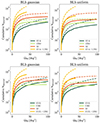 |
Fig. 15. Cumulative number of GW detections (dashed lines) and corresponding KN counterpart detections by Rubin (solid lines) as a function of the sky localisation for upgrade configurations of the current detectors; LVKI and 3A#. As a comparison, we show ET alone and in a network with LVKI. The top panels refer to ET-Δ, while the bottom panels to ET-2L. The shown results are obtained using the fiducial population, the BLh EOS, both the uniform and Gaussian NS mass distributions, and 1ep strategy. |
Number of joint detections by Rubin operating in synergy with current generation detectors (LVKI) and their upgrade (3A#).
The upper panels of Fig. 15 show that for both NS mass distributions, the network of current detectors (LVKI) and the network of LIGO upgrade (3A#) outperforms ET-triangle operating as a single observatory in terms of sky-localisation capabilities for events localised better than 100 deg2. This is reflected in the joint GW/KN detection numbers. Comparing Table 5 and Table 4, we find that Rubin operating with LVKI can detect 60–80% (10–30%) more KNe than ET-triangle as a single observatory for the uniform (Gaussian) NS mass distribution, with a larger increment in the case of APR4 than the BLh EOS. Rubin, operating together with 3A#, is able to detect a factor 3–4 more KNe compared to Rubin with ET-triangle. Interestingly, the lower panels of Fig. 15 show that ET-2L alone outperforms LVKI and approaches the performance of 3A# in sky localisation. In the case of both the triangle and 2L, including ET in a network of current detectors (ET+LVKI) vastly outperforms LVKI and 3A#. Rubin operating with ET+LVKI detects a factor 3–4 more events than 3A#, following up events localised within ΔΩ = 40 deg2. Consistent results are obtained for the APR4 EOS (see Fig. E.7).
Fig. 16 shows the comparative performance of the ET compared to the LVKI, 3A#, and ET+LVKI networks in estimating the relative uncertainty on the luminosity distance. Focusing on the events with relative errors smaller than 10%, ET-triangle (top panels) operating alone performs better than LVKI and 3A# by showing a tail of detections with tiny uncertainties where neither LVKI nor 3A# are capable of the same performance. In the case of ET-2L (bottom panels), ET alone largely outperforms LVKI and 3A#. ET, LVKI and 3A# are vastly outperformed by ET operating in a network with current detectors. ET+LVKI provides almost an order of magnitude more detections with relative errors smaller than 10% than ET alone, LVKI and 3A#. It provides several dozen detections with relative errors of less than 1%. Consistent results are obtained for the APR4 EOS (see Fig. E.8).
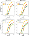 |
Fig. 16. Parameter estimation capability of different GW detectors (ET alone, LVKI, 3A#, ET+LVKI) in terms of relative error in the luminosity distance (ΔdL/dL) corresponding to the GW detections of Figure 15. The top panels refer to ET-Δ, while the bottom panels to ET-2L. Each curve represents a different GW detector network, and the y-axis shows the cumulative number of GW detections with a relative uncertainty on dL smaller than the values in the x-axis. The maximum Ω90 used in the analysis is set at 100 deg2 for each GW network, except for ET+LVKI for which it is set at 40 deg2. The shown results are obtained using the fiducial population, the BLh EOS, both the uniform and Gaussian NS mass distributions, and 1ep strategy. |
4.4. Rubin observations with longer exposures
To explore possible improvements in Rubin's efficiency for detecting KNe, we evaluated the perspectives with an alternative strategy that increases the exposure time for each pointing from 600 s of our nominal strategy to 1200 s. Using the same mosaic strategy with observations in two epochs and in the g and i filters, the time needed for Rubin to follow up all selected events in the footprint using deeper exposures of 1200 s doubles the budget of our nominal strategy. Fig. 17 shows the cumulative number of KN and KN+GRB counterpart detections obtained with 1200 s exposures as a function of the redshift for ET alone, ET+LVKI, and ET+CE for both the triangle and 2L geometries. The plots show the results obtained for the fiducial population, BLh EOS, the NS uniform and Gaussian mass distributions. For comparison, the plots also show the cumulative numbers obtained for the nominal observational strategy (600 s) using thinner lines. We use a sky-localisation threshold of 100 deg2 to select the events to be followed-up for ET alone, of 20 deg2 for ET+LVKI, and 5 deg2 for ET+CE. Equivalent plots for APR4 EOS are shown in Fig. E.9 in Appendix E.
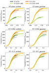 |
Fig. 17. Cumulative number of KN and KN+GRB counterpart detections obtained as a function of the redshift for ET for both ET-triangle and 2L. The thick lines indicate the 1200 s exposure strategy and the thin lines the 600 s exposure. The detections were obtained following up all the events with a sky localisation smaller than 100 deg2 for ET alone (top panels), 20 deg2 for ET+LVKI (middle panels) and 5 deg2 for ET+1CE (bottom panels). The left panels show the results obtained for the uniform NS mass distribution, while the right panels show the ones obtained for the NS Gaussian distribution. All plots refer to the BLh EOS. |
For ET operating as a single observatory (selecting GW alerts with sky localisation < 100 deg2), there is an increase of about 15–20% for the KN detections and 10–15% for the KN+GRB detections both for the triangle and 2L. The observational time increases to 20% of the total Rubin time budget for ET-triangle and 50% for ET-2L. Interestingly, we observe (more prominently for the 2L configuration) that the major increase of KN detections happens at redshifts larger than 0.2, showing an increase in Rubin's detection efficiency at larger z.
The increase at larger redshift is also observed for ET+LVKI and ET+CE. In absolute numbers, an exposure of 1200 s makes the detections increase by 11–23% (13–24%) for the KN (KN+GRB) in the case of ET-triangle (ET-2L) observing in a network with LVKI using 21–34% (28–44%) of the Rubin total observational time. For ET+CE, the increase in the number of detections is 7–20% (10–24%) for the KN (KN+GRB) for the ET-Δ (ET-2L). The required observational time is limited to 8–14% for the ET-triangle and 10–18% for the ET-2L.
For all cases analysed, the longer exposure increases the number of joint optical/GW detections. Although the increase is limited in absolute number to less than 25%, it concentrates at relatively high redshifts allowing a good number of detection at redshifts otherwise inaccessible or with low detection numbers. This is crucial for studies requiring access to high z, such as cosmological parameter estimation.
5. Summary and conclusions
In this work, we explored the prospects of multi-messenger astronomy in the ET era by evaluating the number of detections of KNe and GRB optical afterglows associated with BNS mergers. We considered ET operating as a single observatory or within a network of current or next-generation GW detectors, and observing in synergy with Rubin.
Starting from populations of BNS mergers up to z = 1 generated by population synthesis codes, we conducted 64 simulations over ten years of observations to compute the detection capabilities and parameter estimation by ET, ET+LVKI, ET+1CE, and ET+2CE, considering two possible configurations for ET (triangular with 10 km arms or 2L with 15 km arms). To account for present uncertainties in the local merger rate, NS mass distribution, NS EOS, and KN modelling, we considered a pessimistic and a fiducial BNS merger population with local merger rates ℛBNS=[23, 107] Gpc−3 yr−1, two NS mass distributions (uniform and Gaussian), and two EOSs (APR4 and BLh). The APR4 (BLh) EOS reproduces more (less) compact NSs.
We evaluated the properties of the ejecta for each BNS merger based on the system progenitor properties and we associated each merger with an optical light curve. We calibrated the KN ejecta components based on the results of numerical-relativity simulations targeted to GW170817 and GW190425, introducing new fitting formulas, and modelled the impact of prompt-collapse on the properties of the ejecta. Taking into account the KN ejecta from high-mass BNS mergers, based on the results of GW190425-targeted numerical relativity simulations, makes our population of KNe including fainter and faster-evolving light curves compared to models calibrated using only GW170817-targeted numerical relativity simulations or AT2017gfo data (Fig. C.4 in Appendix C). We also highlight that in the case of a uniform NS mass distribution, we account for the possibility of having highly asymmetric binaries (q∼0.5−0.7). These systems eject a large amount of matter (≳0.02 M⊙) from the tidally disrupted disc, leading to the formation of bright KNe.
To reproduce a realistic scenario, we also added the afterglow emission from the relativistic jet of typical short GRBs. The light curves were corrected for the Galactic extinction based on the source position. We then implemented a realistic follow-up strategy with Rubin, including Rubin's accessible sky, average seeing, slewing and filter change times, and night-day duty cycle.
Our findings indicate that ET already operating as a single observatory will enable detections of a large number of KNe in the range of 10–100 per year, with uncertainties firstly dominated by the local BNS merger rate, then by the ET configuration (triangle versus 2L), and finally dependent on the modelling of NS mass distribution, EOS, and KN microphysics. The number of KN multi-messenger detections significantly increases when ET is operating in a network with current or next-generation detectors up to several hundreds of KNe per year.
In the following, we provide a summary of major results from our study:
-
ET as a single detector will increase the number of BNS merger detections of two orders of magnitude with respect to the current detectors (LVKI) for mergers happening within z<1. Our analysis shows the rate of GW detections is enhanced by 70−90% when ET operates with one or two CEs, whereas the inclusion of LVKI results in a modest 3% increase.
-
ET as a single observatory is able to localise long signals, such as the BNS ones, thanks to the imprint of the Earth rotation in the inspiral signal lasting long in the ET observable band, which starts at relatively low frequencies. However, the number of well-localised events dramatically increases when ET operates in a network of GW detectors. For the fiducial population, the number of events localised better than 100 deg2 up to z = 1 increases from a few hundred per year to several thousand when ET operates with LVKI. Thousands of events per year localised better than 10 deg2 are detected by ET observing in a network with CE.
-
The increase of well-localised events of ET+LVKI makes the detected optical counterparts by Rubin increase by an order of magnitude than ET operating as a single observatory. However, the further increase of detections when Rubin operates with ET+CE does not correspond to the increase of well-localised events but it is limited to a factor of a few. This is mainly due to the Rubin detection efficiency associated with our strategy which already drops significantly at redshifts larger than 0.3. This makes it impossible to gain from the improved localisation accuracy at higher z provided by ET+CE because Rubin's sensitivity is not sufficient to detect KN emission (whereas systems producing an optical afterglow from a jet are observable).
-
The use of deeper Rubin observations (and thus spending more Rubin's time for the follow-up) does not dramatically increase the absolute numbers of detections but interestingly significantly increases the probability of detecting KNe at larger z. To limit the amount of Rubin time required when ET will operate with CE, it will be crucial to select the events to be followed up by prioritising them on the basis of specific scientific targets to achieve. The selection will need to use source parameters beyond the sky-localisation accuracy (e.g. distance, SNR, masses).
-
The combination of sky-localisation capabilities by the GW network and the KN detection efficiency by Rubin makes the networks of current GW detectors (LVKI) and a possible scenario of their upgrades (3A#) outperforming ET-triangle as a single observatory; operating with 3A#, Rubin can detect a factor 3–4 more KNe than ET-triangle. The better sky localisation of ET-2L with respect to ET-triangle makes ET-2L outperform LVKI and approach the performance of 3A#. However, it is important to underline that ET (both geometries) enables us to better estimate crucial parameters such as the source distances. ET+LVKI significantly outperforms LVKI and 3A# in terms of number of joint detections and parameter estimation.
-
The dominant source of uncertainty in the GW detection rate is the still uncertain local BNS merger rate and its evolution with redshift. Since we limit our analysis to events with z<1, the shape of the evolution is expected to be similar for different populations, as shown in Santoliquido et al. (2021), and the main uncertainty thus remains associated with the normalization. The difference in the normalization of our fiducial and pessimistic populations is consistent with the local merger rate range as constrained by current GW detectors, and gives the magnitude of this uncertainty. Another source of uncertainty on the detection rate is given by the poor knowledge of the NS mass distribution. Here, we find that a uniform distribution leads to 20−25% more detections than a Gaussian distribution. On the contrary, the EOS has a small impact (less than 5%) on the number of detections.
-
The uncertainty in the absolute number of KNe detections is also dominated by the poorly constrained local rate of BNS mergers. The NS mass distribution, EOS, and KNe modelling impact the detection rates, albeit to a lesser extent. These factors interplay in complex ways, making their individual effects challenging to disentangle. In the case of a Gaussian NS mass distribution, the BLh EOS (with nuclear factor
 ) yields more KN detections than APR4 (
 ) with an increase ranging between 20% and 60% depending on the selected GW network of detectors. Conversely, when adopting a uniform NS mass distribution, the scenario reverses. In this case, KNe detections under the APR4 framework (
 ) exceed those predicted under the BLh framework (
 ) by 10–20%, varying with the GW network configuration.
 -
Once the jet's optical afterglow emission is included, the rate of multi-messenger detections further increases, especially for the GW network ET+2CE. This network can localise the sources at larger redshifts where the afterglow (intrinsically brighter than the KN emission) is detectable. Such an increase varies with the GW detector networks, the NS mass distribution and EOS, and the KN modelling, ranging between 5% and 30% for the fiducial BNS merger rate, and between 10% and 50% for the pessimistic one.
-
ET, especially in networks with next-generation GW observatories, will generate an extremely large number of alerts, making it prohibitive to follow up on every one of them. Here, we propose a simple observational strategy based on sky-localization selection, however, searches can be further optimised to be effective based on specific science cases. The selection and prioritization of alerts to be followed will require incorporating additional information about the source parameters. For instance, nuclear physics studies could focus on golden SNR events, which offer the best parameter estimates; cosmological studies could prioritize alerts based on source distance estimates; and studies of ejecta physics and nucleosynthesis could be guided by component masses. In the latter case, our study provides predictions of the expected ejecta and light curves based on the component masses. To explore science-case-dependent observational strategies based on source parameter estimates, we make available to the community the catalogues containing the uncertainty estimate for all the source parameters for the BNS merger populations and networks presented in this paper14.
Our study provides a comprehensive overview of KN multi-messenger prospects for the next-generation GW observatories operating with innovative optical wide field-of-view observatories, such as the Vera Rubin Observatory. It makes a significant step forwards in quantifying theoretical uncertainties affecting predictions on KNe multi-messenger detections, which need to be taken into account to devise robust observational strategies. As highlighted in the previous paragraphs, the largest source of uncertainty is given by the rate of BNS mergers. In addition to that, the mass distribution within BNS systems is still poorly constrained on both the sides of observational data and population synthesis simulations. By using either a Gaussian or a uniform NS mass distribution, our analysis explores the two extreme scenarios, including very asymmetric BNS systems in the case of uniform mass distribution. Both the total mass and the binary mass ratio of the two NSs have a profound impact on the brightness and time evolution of the KN light curves. Further theoretical studies are needed to understand how frequent these asymmetric systems (q≲0.7) are in the BNS mergers population. The time that bridges current detectors to the ET era is expected to improve our knowledge of BNS and the associated KN emission which are currently mainly constrained by only two BNS merger detections in GWs and a single KN associated with GW170817. Upcoming observations will provide important information (on BNS merger rate, NS properties, KN emission) to overcome current analysis limitations.
Data availability
The output data of the GW simulations presented in this work (see Sects. 2.3 and 4.1) are publicly available on Zenodo at Dupletsa et al. (2024). GWFish is publicly available on Github: the version used in this work is the commit CF26D3C in the main branch.
Acknowledgments
M.B. and E.L. acknowledge financial support from the Italian Ministry of University and Research (MUR) for the PRIN grant METE under contract no. 2020KB33TP. M.B. and F.S. acknowledge financial support from the AHEAD2020 project (grant agreement n. 871158). E.L. acknowledges funding by the European Union – NextGenerationEU RFF M4C2 1.1 PRIN 2022 project 2022RJLWHN URKA. This work has received funding from the European Research Council (ERC) under the European Union's Horizon 2020 research and innovation programme, Grant agreement No. 770017. M.M. acknowledges support from the Deutsche Forschungsgemeinschaft (DFG) under Germany's Excellence Strategy EXC 2181/1-390900948. We acknowledge useful discussion with M. Arca Sedda, S. Borhanian, A. Colombo, M. Drago, G. Ghirlanda, F. Gulminelli, D. Logoteta, A. Maselli, J. Tissino. We acknowledge Stefano Bagnasco, Federica Legger, Sara Vallero, and the INFN Computing Center of Turin for providing support and computational resources.
The official documentation from the Rubin Survey Cadence Optimizing Committee is available at this link.
SEVN is publicly available at this link.
The sensitivity curves are available at this link.
GWFish is publicly available on GitHub.
The sky-localisation region at 1σ was obtained using the uncertainties on RA and DEC. To obtain the X% level of sky localisation one should multiply the value obtained by GWFish by  . This results in a multiplicative factor of ∼4.6 when considering 90% confidence level.
The xkn framework is publicly available on GitHub.
We use as Rubin's visible sky the EuclidOverlapFootprint of the rubin_sim module available on GitHub.
Using sunrise maps available at this link.
The overhead associated with the slewing time to cover the mosaic was defined conservatively, calculated for a sky localisation of 100 deg2 and also applied for events detected with a better localisation.
More details are provided in this LSST technote. In particular, we used the m5 values from the LSST Operations Simulator.
This is a conservative assumption since having the real localization probability distribution provided by a full posteriors analysis would make the observational strategy more effective, starting the mosaic from the tiles having a higher probability to contain the source.
An exception is noted for the ET operating independently, where a Gaussian mass distribution results in more detections than a uniform distribution within the APR4 framework.
The parameter estimation catalogues are publicly available at this link.
References
- Abbott, B. P., Abbott, R., Abbott, T. D., et al. 2017a, Phys. Rev. Lett., 119, 161101 [Google Scholar]
- Abbott, B. P., Abbott, R., Abbott, T. D., et al. 2017b, ApJ, 848, L12 [Google Scholar]
- Abbott, B. P., Abbott, R., Abbott, T. D., et al. 2017c, Nature, 551, 85 [Google Scholar]
- Abbott, B. P., Abbott, R., Abbott, T. D., et al. 2018, Phys. Rev. Lett., 121, 161101 [Google Scholar]
- Abbott, B. P., Abbott, R., Abbott, T. D., et al. 2020a, ApJ, 892, L3 [NASA ADS] [CrossRef] [Google Scholar]
- Abbott, B. P., Abbott, R., Abbott, T. D., et al. 2020b, Liv. Rev. Relat., 23, 3 [NASA ADS] [Google Scholar]
- Abbott, R., Abbott, T. D., Acernese, F., et al. 2023, Phys. Rev. X, 13, 011048 [NASA ADS] [Google Scholar]
- Ackley, K., Adya, V. B., Agrawal, P., et al. 2020, PASA, 37, e047 [NASA ADS] [CrossRef] [Google Scholar]
- Akmal, A., Pandharipande, V. R., & Ravenhall, D. G. 1998, Phys. Rev. C, 58, 1804 [Google Scholar]
- Akutsu, T., Ando, M., Arai, K., et al. 2019, Class. Quantum Gravity, 36, 165008 [Google Scholar]
- Andreoni, I., Anand, S., Bianco, F. B., et al. 2019, PASP, 131, 068004 [NASA ADS] [CrossRef] [Google Scholar]
- Andreoni, I., Coughlin, M. W., Almualla, M., et al. 2022a, ApJS, 258, 5 [Google Scholar]
- Andreoni, I., Margutti, R., Salafia, O. S., et al. 2022b, ApJS, 260, 18 [NASA ADS] [CrossRef] [Google Scholar]
- Antoniadis, J., Freire, P. C. C., Wex, N., et al. 2013, Science, 340, 448 [Google Scholar]
- Ascenzi, S., Coughlin, M. W., Dietrich, T., et al. 2019, MNRAS, 486, 672 [Google Scholar]
- Bailes, M., Berger, B. K., Brady, P. R., et al. 2021, Nat. Rev. Phys., 3, 344 [NASA ADS] [CrossRef] [Google Scholar]
- Banerjee, B., Oganesyan, G., Branchesi, M., et al. 2023, A&A, 678, A126 [NASA ADS] [CrossRef] [EDP Sciences] [Google Scholar]
- Barbieri, C., Salafia, O. S., Colpi, M., Ghirlanda, G., & Perego, A. 2021, A&A, 654, A12 [NASA ADS] [CrossRef] [EDP Sciences] [Google Scholar]
- Barnes, J., & Kasen, D. 2013, ApJ, 775, 18 [NASA ADS] [CrossRef] [Google Scholar]
- Bauswein, A., Goriely, S., & Janka, H. T. 2013, ApJ, 773, 78 [NASA ADS] [CrossRef] [Google Scholar]
- Baym, G., Pethick, C., & Sutherland, P. 1971, ApJ, 170, 299 [NASA ADS] [CrossRef] [Google Scholar]
- Bernuzzi, S., Breschi, M., Daszuta, B., et al. 2020, MNRAS, 497, 1488 [Google Scholar]
- Bhattacharjee, S., Banerjee, S., Bhalerao, V., et al. 2024, MNRAS, 528, 4255 [NASA ADS] [CrossRef] [Google Scholar]
- Bianco, F. B., Drout, M. R., Graham, M. L., et al. 2019, PASP, 131, 068002 [Google Scholar]
- Bianco, F. B., Ivezić, Ž., Jones, R. L., et al. 2021, ApJS, 258, 1 [Google Scholar]
- Bombaci, I., & Logoteta, D. 2018, A&A, 609, A128 [EDP Sciences] [Google Scholar]
- Branchesi, M., Maggiore, M., Alonso, D., et al. 2023, JCAP, 2023, 068 [CrossRef] [Google Scholar]
- Breschi, M., Perego, A., Bernuzzi, S., et al. 2021, MNRAS, 505, 1661 [NASA ADS] [CrossRef] [Google Scholar]
- Breschi, M., Gamba, R., Carullo, G., et al. 2024, A&A, 689, A51 [NASA ADS] [CrossRef] [EDP Sciences] [Google Scholar]
- Burgay, M., D’Amico, N., Possenti, A., et al. 2003, Nature, 426, 531 [NASA ADS] [CrossRef] [Google Scholar]
- Camilletti, A., Chiesa, L., Ricigliano, G., et al. 2022, MNRAS, 516, 4760 [CrossRef] [Google Scholar]
- Chen, H. -Y., Cowperthwaite, P. S., Metzger, B. D., & Berger, E. 2021, ApJ, 908, L4 [NASA ADS] [CrossRef] [Google Scholar]
- Colombo, A., Salafia, O. S., Gabrielli, F., et al. 2022, ApJ, 937, 79 [NASA ADS] [CrossRef] [Google Scholar]
- Cowperthwaite, P. S., Villar, V. A., Scolnic, D. M., & Berger, E. 2019, ApJ, 874, 88 [Google Scholar]
- Damour, T., Nagar, A., & Villain, L. 2012, Phys. Rev. D, 85, 123007 [NASA ADS] [CrossRef] [Google Scholar]
- Day, B. D. 1967, Rev. Mod. Phys., 39, 719 [Google Scholar]
- Dietrich, T., & Ujevic, M. 2017, Class. Quantum Gravity, 34, 105014 [Google Scholar]
- Dietrich, T., Samajdar, A., Khan, S., et al. 2019, Phys. Rev. D, 100, 044003 [NASA ADS] [CrossRef] [Google Scholar]
- Dietrich, T., Coughlin, M. W., Pang, P. T. H., et al. 2020, Science, 370, 1450 [Google Scholar]
- Douchin, F., & Haensel, P. 2001, A&A, 380, 151 [NASA ADS] [CrossRef] [EDP Sciences] [Google Scholar]
- Dudi, R., Adhikari, A., Brügmann, B., et al. 2022, Phys. Rev. D, 106, 084039 [Google Scholar]
- Dupletsa, U., Harms, J., Banerjee, B., et al. 2023, Astron. Comput., 42, 100671 [NASA ADS] [CrossRef] [Google Scholar]
- Dupletsa, U., Santoliquido, F., Branchesi, M., & Loffredo, E. 2024, https://doi.org/10.5281/zenodo.13850416 [Google Scholar]
- Eichler, D., Livio, M., Piran, T., & Schramm, D. N. 1989, Nature, 340, 126 [NASA ADS] [CrossRef] [Google Scholar]
- Evans, M., Adhikari, R. X., Afle, C., et al. 2021, arXiv e-prints [arXiv:2109.09882] [Google Scholar]
- Evans, M., Corsi, A., Afle, C., et al. 2023, arXiv e-prints [arXiv:2306.13745] [Google Scholar]
- Favata, M. 2014, Phys. Rev. Lett., 112, 101101 [NASA ADS] [CrossRef] [Google Scholar]
- Fong, W., Berger, E., Margutti, R., & Zauderer, B. A. 2015, ApJ, 815, 102 [NASA ADS] [CrossRef] [Google Scholar]
- Freiburghaus, C., Rosswog, S., & Thielemann, F. K. 1999, ApJ, 525, L121 [NASA ADS] [CrossRef] [Google Scholar]
- Fritschel, P., Kuns, K., Driggers, J., et al. 2022, Tech. Rep. T2200287 (LIGO) [Google Scholar]
- Fryer, C. L., Belczynski, K., Wiktorowicz, G., et al. 2012, ApJ, 749, 91 [Google Scholar]
- Ghirlanda, G., Salafia, O. S., Paragi, Z., et al. 2019, Science, 363, 968 [NASA ADS] [CrossRef] [Google Scholar]
- Giacobbo, N., & Mapelli, M. 2020, ApJ, 891, 141 [NASA ADS] [CrossRef] [Google Scholar]
- Green, G. 2018, J. Open Source Softw., 3, 695 [NASA ADS] [CrossRef] [Google Scholar]
- Grimm, S., & Harms, J. 2020, Phys. Rev. D, 102, 022007 [NASA ADS] [CrossRef] [Google Scholar]
- Grossman, D., Korobkin, O., Rosswog, S., & Piran, T. 2014, MNRAS, 439, 757 [NASA ADS] [CrossRef] [Google Scholar]
- Gupta, I., Afle, C., Arun, K. G., et al. 2024, Class. Quantum Gravity, 41, 245001 [Google Scholar]
- Hempel, M., & Schaffner-Bielich, J. 2010, Nucl. Phys. A, 837, 210 [Google Scholar]
- Hendriks, K., Yi, S. -X., & Nelemans, G. 2023, A&A, 672, A74 [NASA ADS] [CrossRef] [EDP Sciences] [Google Scholar]
- Henkel, A., Foucart, F., Raaijmakers, G., & Nissanke, S. 2023, Phys. Rev. D, 107, 063028 [Google Scholar]
- Hinderer, T. 2008, ApJ, 677, 1216 [NASA ADS] [CrossRef] [Google Scholar]
- Hobbs, G., Lorimer, D. R., Lyne, A. G., & Kramer, M. 2005, MNRAS, 360, 974 [Google Scholar]
- Iacovelli, F., Mancarella, M., Mondal, C., et al. 2023, Phys. Rev. D, 108, 122006 [CrossRef] [Google Scholar]
- Iorio, G., Mapelli, M., Costa, G., et al. 2023, MNRAS, 524, 426 [NASA ADS] [CrossRef] [Google Scholar]
- Ivezić, Ž., Kahn, S. M., Tyson, J. A., et al. 2019, ApJ, 873, 111 [Google Scholar]
- Kann, D. A., Klose, S., Zhang, B., et al. 2011, ApJ, 734, 96 [NASA ADS] [CrossRef] [Google Scholar]
- Kasen, D., & Barnes, J. 2019, ApJ, 876, 128 [Google Scholar]
- Kasen, D., Badnell, N. R., & Barnes, J. 2013, ApJ, 774, 25 [NASA ADS] [CrossRef] [Google Scholar]
- Kasen, D., Metzger, B., Barnes, J., Quataert, E., & Ramirez-Ruiz, E. 2017, Nature, 551, 80 [Google Scholar]
- Kashyap, R., Das, A., Radice, D., et al. 2022, Phys. Rev. D, 105, 103022 [NASA ADS] [CrossRef] [Google Scholar]
- Khan, S., Husa, S., Hannam, M., et al. 2016, Phys. Rev. D, 93, 044007 [Google Scholar]
- Kiziltan, B., Kottas, A., De Yoreo, M., & Thorsett, S. E. 2013, ApJ, 778, 66 [NASA ADS] [CrossRef] [Google Scholar]
- Kroupa, P. 2001, MNRAS, 322, 231 [NASA ADS] [CrossRef] [Google Scholar]
- Krüger, C. J., & Foucart, F. 2020, Phys. Rev. D, 101, 103002 [CrossRef] [Google Scholar]
- Kulkarni, S. R. 2005, arXiv e-prints [arXiv:astro-ph/0510256] [Google Scholar]
- Kyutoku, K., Fujibayashi, S., Hayashi, K., et al. 2020, ApJ, 890, L4 [Google Scholar]
- Lattimer, J. M., & Steiner, A. W. 2014, ApJ, 784, 123 [Google Scholar]
- Levan, A. J., Gompertz, B. P., Salafia, O. S., et al. 2024, Nature, 626, 737 [NASA ADS] [CrossRef] [Google Scholar]
- Li, L. -X., & Paczyński, B. 1998, ApJ, 507, L59 [NASA ADS] [CrossRef] [Google Scholar]
- LIGO Scientific Collaboration 2018, LIGO Algorithm Library – LALSuite, free 1870 software (GPL), https://doi.org/10.7935/GT1W-FZ16 [Google Scholar]
- Liske, J. 2014, in Thirty Meter Telescope Science Forum, eds. M. Dickinson, & H. Inami, 52 [Google Scholar]
- Logoteta, D., Perego, A., & Bombaci, I. 2021, A&A, 646, A55 [NASA ADS] [CrossRef] [EDP Sciences] [Google Scholar]
- Madau, P., & Fragos, T. 2017, ApJ, 840, 39 [Google Scholar]
- Mainieri, V., Anderson, R. I., Brinchmann, J., et al. 2024, arXiv e-prints [arXiv:2403.05398] [Google Scholar]
- Mapelli, M., Spera, M., Montanari, E., et al. 2020, ApJ, 888, 76 [NASA ADS] [CrossRef] [Google Scholar]
- Marconi, A., Abreu, M., Adibekyan, V., et al. 2022, in Ground-based and Airborne Instrumentation for Astronomy IX, eds. C. J. Evans, J. J. Bryant, & K. Motohara, Society of Photo-Optical Instrumentation Engineers (SPIE) Conference Series, 12184, 1218424 [NASA ADS] [Google Scholar]
- Margalit, B., & Metzger, B. D. 2017, ApJ, 850, L19 [Google Scholar]
- Margutti, R., Cowperthwaite, P., Doctor, Z., et al. 2018, arXiv e-prints [arXiv:1812.04051] [Google Scholar]
- Martin, D., Perego, A., Arcones, A., et al. 2015, ApJ, 813, 2 [NASA ADS] [CrossRef] [Google Scholar]
- Mei, A., Banerjee, B., Oganesyan, G., et al. 2022, Nature, 612, 236 [NASA ADS] [CrossRef] [Google Scholar]
- Mendoza-Temis, J. d. J., Wu, M. -R., Langanke, K.,, et al. 2015, Phys. Rev. C, 92, 055805 [CrossRef] [Google Scholar]
- Metzger, B. D. 2019, Liv. Rev. Relat., 23, 1 [Google Scholar]
- Metzger, B. D., & Fernández, R. 2014, MNRAS, 441, 3444 [CrossRef] [Google Scholar]
- Metzger, B. D., Martínez-Pinedo, G., Darbha, S., et al. 2010, MNRAS, 406, 2650 [NASA ADS] [CrossRef] [Google Scholar]
- Miller, M. C., Lamb, F. K., Dittmann, A. J., et al. 2019, ApJ, 887, L24 [Google Scholar]
- Miller, M. C., Lamb, F. K., Dittmann, A. J., et al. 2021, ApJ, 918, L28 [NASA ADS] [CrossRef] [Google Scholar]
- Möller, P., Sierk, A. J., Ichikawa, T., & Sagawa, H. 2016, At. Data Nucl. Data Tables, 109, 1 [CrossRef] [Google Scholar]
- Nedora, V., Bernuzzi, S., Radice, D., et al. 2019, ApJ, 886, L30 [NASA ADS] [CrossRef] [Google Scholar]
- Nedora, V., Bernuzzi, S., Radice, D., et al. 2021, ApJ, 906, 98 [NASA ADS] [CrossRef] [Google Scholar]
- Nedora, V., Schianchi, F., Bernuzzi, S., et al. 2022, Class. Quantum Gravity, 39, 015008 [NASA ADS] [CrossRef] [Google Scholar]
- Oertel, M., Hempel, M., Klähn, T., & Typel, S. 2017, Rev. Mod. Phys., 89, 015007 [Google Scholar]
- Özel, F., & Freire, P. 2016, ARA&A, 54, 401 [Google Scholar]
- Özel, F., Psaltis, D., Narayan, R., & Santos Villarreal, A. 2012, ApJ, 757, 55 [Google Scholar]
- Patricelli, B., Bernardini, M. G., Mapelli, M., et al. 2022, MNRAS, 513, 4159 [NASA ADS] [CrossRef] [Google Scholar]
- Perego, A., Rosswog, S., Cabezon, R., et al. 2014, MNRAS, 443, 3134 [NASA ADS] [CrossRef] [Google Scholar]
- Perego, A., Radice, D., & Bernuzzi, S. 2017, ApJ, 850, L37 [NASA ADS] [CrossRef] [Google Scholar]
- Perego, A., Logoteta, D., Radice, D., et al. 2022, Phys. Rev. Lett., 129, 032701 [NASA ADS] [CrossRef] [Google Scholar]
- Petrov, P., Singer, L. P., Coughlin, M. W., et al. 2022, ApJ, 924, 54 [NASA ADS] [CrossRef] [Google Scholar]
- Pian, E., D’Avanzo, P., Benetti, S., et al. 2017, Nature, 551, 67 [Google Scholar]
- Pinto, P. A., & Eastman, R. G. 2000, ApJ, 530, 744 [Google Scholar]
- Planck Collaboration VI. 2020, A&A, 641, A6 [Erratum: A&A, 652, C4 (2021)] [NASA ADS] [CrossRef] [EDP Sciences] [Google Scholar]
- Raaijmakers, G., Nissanke, S., Foucart, F., et al. 2021a, ApJ, 922, 269 [NASA ADS] [CrossRef] [Google Scholar]
- Raaijmakers, G., Greif, S. K., Hebeler, K., et al. 2021b, ApJ, 918, L29 [NASA ADS] [CrossRef] [Google Scholar]
- Radice, D., & Bernuzzi, S. 2023, ApJ, 959, 46 [NASA ADS] [CrossRef] [Google Scholar]
- Radice, D., Perego, A., Hotokezaka, K., et al. 2018, ApJ, 869, 130 [Google Scholar]
- Radice, D., Ricigliano, G., Bhattacharya, M., et al. 2024, MNRAS, 528, 5836 [Google Scholar]
- Ragosta, F., Ahumada, T., Piranomonte, S., et al. 2024, ApJ, 966, 214 [Google Scholar]
- Rastinejad, J. C., Gompertz, B. P., Levan, A. J., et al. 2022, Nature, 612, 223 [NASA ADS] [CrossRef] [Google Scholar]
- Ricigliano, G., Perego, A., Borhanian, S., et al. 2024, MNRAS, 529, 647 [NASA ADS] [CrossRef] [Google Scholar]
- Riley, T. E., Watts, A. L., Bogdanov, S., et al. 2019, ApJ, 887, L21 [Google Scholar]
- Ronchini, S., Branchesi, M., Oganesyan, G., et al. 2022, A&A, 665, A97 [NASA ADS] [CrossRef] [EDP Sciences] [Google Scholar]
- Rosswog, S., Feindt, U., Korobkin, O., et al. 2017, Class. Quantum Gravity, 34, 104001 [CrossRef] [Google Scholar]
- Ryan, G., van Eerten, H., Piro, L., & Troja, E. 2020, ApJ, 896, 166 [CrossRef] [Google Scholar]
- Sana, H., de Mink, S. E., de Koter, A., et al. 2012, Science, 337, 444 [Google Scholar]
- Santoliquido, F., Mapelli, M., Bouffanais, Y., et al. 2020, ApJ, 898, 152 [Google Scholar]
- Santoliquido, F., Mapelli, M., Giacobbo, N., Bouffanais, Y., & Artale, M. C. 2021, MNRAS, 502, 4877 [NASA ADS] [CrossRef] [Google Scholar]
- Sarin, N., & Lasky, P. D. 2022, PASA, 39, e007 [NASA ADS] [CrossRef] [Google Scholar]
- Schlafly, E. F., & Finkbeiner, D. P. 2011, ApJ, 737, 103 [Google Scholar]
- Schlegel, D. J., Finkbeiner, D. P., & Davis, M. 1998, ApJ, 500, 525 [Google Scholar]
- Schneider, A. S., Roberts, L. F., & Ott, C. D. 2017, Phys. Rev. C, 96, 065802 [Google Scholar]
- Scolnic, D., Kessler, R., Brout, D., et al. 2018, ApJ, 852, L3 [NASA ADS] [CrossRef] [Google Scholar]
- Sekiguchi, Y., Kiuchi, K., Kyutoku, K., Shibata, M., & Taniguchi, K. 2016, Phys. Rev. D, 93, 124046 [NASA ADS] [CrossRef] [Google Scholar]
- Setzer, C. N., Biswas, R., Peiris, H. V., et al. 2019, MNRAS, 485, 4260 [CrossRef] [Google Scholar]
- Shah, V. G., Narayan, G., Perkins, H. M. L., et al. 2024, MNRAS, 528, 1109 [Google Scholar]
- Siegel, D. M., & Metzger, B. D. 2017, Phys. Rev. Lett., 119, 231102 [NASA ADS] [CrossRef] [Google Scholar]
- Smartt, S. J., Chen, T. W., Jerkstrand, A., et al. 2017, Nature, 551, 75 [NASA ADS] [CrossRef] [Google Scholar]
- Spera, M., Mapelli, M., Giacobbo, N., et al. 2019, MNRAS, 485, 889 [Google Scholar]
- Steiner, A. W., Hempel, M., & Fischer, T. 2013, ApJ, 774, 17 [NASA ADS] [CrossRef] [Google Scholar]
- Troja, E., Fryer, C. L., O’Connor, B., et al. 2022, Nature, 612, 228 [NASA ADS] [CrossRef] [Google Scholar]
- Typel, S., Röpke, G., Klähn, T., Blaschke, D., & Wolter, H. H. 2010, Phys. Rev. C, 81, 015803 [NASA ADS] [CrossRef] [Google Scholar]
- Villar, V. A., et al. 2017, ApJ, 851, L21 [CrossRef] [Google Scholar]
- Wollaeger, R. T., Korobkin, O., Fontes, C. J., et al. 2018, MNRAS, 478, 3298 [NASA ADS] [CrossRef] [Google Scholar]
- Wu, M. -R., Fernández, R., Martínez-Pinedo, G., & Metzger, B. D. 2016, MNRAS, 463, 2323 [NASA ADS] [CrossRef] [Google Scholar]
- Yang, Y. -H., Troja, E., O’Connor, B., et al. 2024, Nature, 626, 742 [NASA ADS] [CrossRef] [Google Scholar]
- Zhu, Y. L., Lund, K. A., Barnes, J., et al. 2021, ApJ, 906, 94 [CrossRef] [Google Scholar]
Appendix A: Properties of the BNS populations
Here we present the properties of the BNS populations analysed in our work. Figs. A.1 and A.2 illustrate the distributions of NS mass and tidal deformability (as defined in Eq. (3)), as well as BNS mass ratios and chirp masses for the populations with Gaussian and uniform mass distribution, respectively.
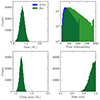 |
Fig. A.1. Distribution of NS masses and tidal deformability defined in Eq. (3) (top) and BNS chirp masses and mass ratios (bottom) corresponding to the population with α = 1.0 and Gaussian mass distribution, for APR4 and BLh EOSs. |
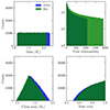 |
Fig. A.2. Distribution of NS masses and tidal deformability defined in Eq. (3) (top) and BNS chirp masses and mass ratios (bottom) corresponding to the population with α = 1.0 and uniform mass distribution, for APR4 and BLh EOSs. |
Notably, when comparing the two EOSs, the most significant differences are observed in the tidal deformability distributions. The BLh EOS shows generally larger tidal deformability values compared to APR4. For the uniform mass distribution (see Fig. A.2), the maximum masses attained are larger for APR4, leading to subtle variations in both the mass ratio and chirp mass distributions between APR4 and BLh.
Furthermore, a comparison between the Gaussian and uniform mass distribution populations (Fig. A.1 and Fig. A.2) reveals marked differences in the distributions of tidal deformability, mass ratio, and chirp mass. Particularly in the population with a uniform mass distribution, we see a broader distribution of chirp masses, extending to almost 2, and mass ratios descending to values as low as 0.5. This indicates a significant presence of asymmetric systems within the uniformly distributed mass population. This has a significant impact on the KN light curves. However, the asymmetric mass ratio of our systems is constructed a posteriori and does not come from the real evolution of the binaries.
Appendix B: GW detectors characteristics
In Table B.1 we summarise the main characteristics of the GW detectors in our simulation set-up. Specifically, we show the arm length, the location (country, latitude and longitude), the minimum frequency used for the analysis, and the adopted sensitivity curve. The sensitivity curves are then shown in Fig. B.1.
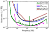 |
Fig. B.1. Sensitivity curves used in the analysis. The ET strain noise is plotted considering a single nested detector, composed of a low-frequency and a high-frequency interferometer. Our analysis takes into account that the triangular-shaped ET consists of three nested detectors, each of them with the same sensitivity curve. |
Detectors list and their main characteristics.
Appendix C: Complements to kilonova modelling
In this section, we provide additional figures and tests complementing the description of our KN modelling from Sect. 2.4.
In Fig. C.1, we show mdyn, vdyn, and mdisc, as defined in Eq. (6)-(8), in the M1−M2 space for the APR4 EOS. See Figs. 2-3 for a comparison with BLh. Fig. C.2 displays the ejecta component masses mC1 and mC2, as defined in Eq. (12) and Eq. (14), in the M1−M2 space for the APR4 EOSs.
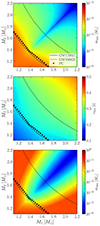 |
Fig. C.1. Mass of the dynamical ejecta (top), velocity of the dynamical ejecta (centre), and mass of the disc (bottom), as defined in Eq. (6)-(8) for the EOS APR4. x and y axes represent the BNS masses M1, M2. The solid and the dashed black lines mark the chirp mass of GW170817 and GW190425, respectively. The triangular markers show the prompt-collapse mass threshold MPC. |
Fig. C.3 presents the KN light curves and their probability distributions in the g and i filters of Rubin. These light curves are calculated for the BNS mergers detected by ET-triangle within 100 deg2 from populations characterised by a common envelope efficiency α = 1.0, uniform NS mass distribution, and BLh (left) and APR4 (right) EOSs. For a comparison with the Gaussian mass distribution, see Fig. 4.
Finally, in Fig. C.4 we compare three relevant cases of our modelled KN light curves for APR4 (red) and BLh (blue) EOSs to AT2017gfo at fixed luminosity distance dL = 100 Mpc and inclination angle ι = 20 deg. Specifically, an average KN (solid lines) is modelled using an equal-mass BNS system with masses at the peak of a Gaussian distribution. Bright KN light curves (dashed lines) arise from a BNS system in the Gaussian mass distribution that produces the most massive disc, while faint KN light curves (dotted lines) correspond to a BNS system that results in the least massive disc. We notice that our population of KNe includes light curves that are significantly fainter than AT2017gfo, originating from BNS mergers that undergo prompt collapse into BH.
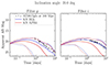 |
Fig. C.4. KNe light curves for BLh (blue lines) and APR4 (red lines) EOSs computed in the g and i filter of Rubin at inclination angle 20 deg, assuming luminosity distance dL = 100 Mpc. KNe light curves correspond to three different BNS systems. Solid lines correspond to M1=M2 = 1.33 M⊙ (the peak of the NS mass distribution); dashed lines correspond to M1 = 1.18 M⊙, M2 = 1.10 M⊙ (the BNS producing the most massive disc); dotted lines correspond to M1=M2 = 1.57 M⊙ (the BNS producing the lightest disc). KNe light curves are compared to AT2017gfo (black diamonds) (Villar 2017) placed at dL = 100 Mpc. |
C.1. Kilonova modelling reproducing AT2017gfo
In Sect. 2.4, we described how we compute the KN light curves given the component masses and the EOS of the BNS system. In this section, we evaluate the effectiveness of our model by assessing its ability to replicate the observed light curve of AT2017gfo, the KN associated with GW170817. We consider two populations of (BNS) mergers over ten years, one obtained using the APR4 EOS and the other the BLh EOS. Both populations adopt a common envelope efficiency α = 1.0 and a Gaussian mass distribution (refer to Sect. 2.1). From each population, we extract binaries whose chirp mass and mass ratio align with those of GW170817, specifically setting Mchirp = 1.186±0.005 and q>0.725. For every selected binary, we compute the corresponding KN light curve (as detailed in Sect. 2.4), assuming a luminosity distance of 40 Mpc and an inclination angle of 20 degrees, akin to GW170817. We then identify the brightest and faintest KNe light curves from each population and compare them with the observed data of AT2017gfo.
Our findings are presented in Fig. C.5, where the observed magnitudes of AT2017gfo in the B, g, r, i, z, and Ks bands are depicted with diamonds (Villar 2017). The lines represent the brightest and the faintest KN light curves for APR4 (dashed lines) and BLh (solid lines). For both the EOSs, the brightest light curves correspond to BNS component masses (M1, M2) = (1.58, 1.17) M⊙, while the faintest to (M1, M2) = (1.37, 1.37) M⊙. Notably, the light curve of AT2017gfo falls between our model's brightest and faintest synthetic KN light curves for both the EOSs, except for the g band, where the brightest light curves match the observations. This comparison demonstrates that our model is capable of reproducing the observations of AT2017gfo for source parameters consistent with GW170817.
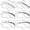 |
Fig. C.5. Comparison between AT2017gfo data (apparent AB magnitude) in the B, g, r, i, z, Ks bands (diamonds) (Villar 2017) and the KN light curves corresponding to the brightest and the faintest KN signals obtained by selecting (BNSs) with chirp mass Mchirp = 1.186±0.005 and binary mass ratio q>0.725 from the population with α = 1.0 and Gaussian mass distribution. Dashed and solid lines correspond to the case of APR4 and BLh, respectively. |
Appendix D: Complements to GW results
Table D.1 gives the number of BNS detected in ten years by several configurations of network detectors for the fiducial population (α = 1). The second and third columns show the numbers for the APR4 EOS and the uniform and Gaussian NS mass distributions, respectively. The fourth and fifth columns show the numbers for the BLh EOS.
Number of BNS mergers detected in ten years by several networks of current and next generation detectors for the fiducial populations (α = 1.0).
Fig. D.1 shows the number of detections in ten years up to redshift z = 1 for the fiducial population (α = 1.0) with the BLh EOS, as in Fig. 7, but assuming the Gaussian NS mass distribution. The total number of detections by the 2L ET is a factor 40% larger than the detections by the ET-triangle. When ET-triangle or 2L shape operates with LVKI, an increase in the number of detections of a few percent is present. A much more significant increase takes place when ET operates with the next-generation detectors. For ET-triangle the number of detections doubles, and for ET-2L increases by about 45% with one CE in the USA, and 60% with one CE in the USA and one CE in Australia.
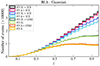 |
Fig. D.1. Ten-year detection distribution as a function of redshift for the eight different networks using the fiducial population (α = 1.0) with BLh EOS and Gaussian mass distribution. |
Figs. D.2, D.3, and D.4 show the number of events localised better than 100, 40, 20, 10, and 1 deg2 by the different detector networks for the fiducial population (α = 1.0) assuming the BLh EOSs and Gaussian NS mass distribution, the APR4 EOSs and uniform NS mass distribution, the APR4 EOSs and Gaussian NS mass distribution, respectively. The left plots refer to ET-triangle and the right ones to ET-2L. It is evident from all the plots the importance of the presence of current detectors which significantly increase of the number of detections and of the redshifts reached by well-localised events. These improvements, as expected, are then largely enhanced with networks of next-generation detectors. In Table D.2 and Table D.3, we list the number of BNS mergers detected within a certain sky-localisation threshold by the triangular and the 2L ET, respectively, operating as a single observatory or in a network of GW detectors.
Number of BNS mergers detected by ET triangular shape with 10 km arms in ten years with a sky localisation better than 100 deg2, 40 deg2, 20 deg2, 10 deg2, and 1 deg2.
Number of BNS mergers detected by the 2L ET with 15 km arms in ten years with a sky localisation better than 100 deg2, 40 deg2, 20 deg2, 10 deg2, and 1 deg2 respectively.
Figs. D.5 and D.6 show the distribution of SNR and uncertainties on the source parameters obtained with GWFish for the fiducial population assuming the Gaussian NS mass distribution with BLh EOS and the uniform NS mass distribution with APR4 EOS, respectively.
Appendix E: Complements to joint GW and optical detection results
Fig. E.1, Fig. E.2 and Fig. E.3 show the time necessary to follow up all the events in the Rubin footprint with a sky localisation smaller than Ω90 (left panels) and the corresponding number of optical detections by Rubin (right panels). Fig. E.1 provides the results obtained for ET-triangle and APR4 EOS, while Fig. E.2 and Fig. E.3 the results obtained for 2L ET and the BLh and APR4 EOSs, respectively. Fig. E.4 shows the joint GW/optical detection efficiency as a function of redshift for the BLh EOS as in Fig. 12 but for the Gaussian NS mass distribution. Fig. E.5 and Fig. E.6 show the detection efficiency for the APR4 EOS considering the uniform NS and Gaussian mass distributions, respectively. Fig. E.7 shows the cumulative number of GW detection and corresponding KN counterparts as a function of the sky localisation for ET, and possible upgrade scenarios of current detectors, LVKI and 3A#, considering the APR4 EOS. Fig. E.8 shows the comparison of the parameter estimation capabilities of ET alone, LVKI, 3A# and ET+LVKI in terms of the relative error on the luminosity distance, considering the APR4 EOS.
Table E.1 lists the number of KN and KN plus GRB optical afterglow detected by Rubin working in synergy with the 2L ET, operating as a single observatory or in a network of GW detectors. In Table E.2, we report the number of KN (KN plus GRB optical afterglow) detections obtained by ET operating in a network with two CEs and Rubin, following events with a sky localisation better than 1 deg2. A comparison with Table 4 and Table E.1, where the cut on sky localisation is set to 5 deg2, shows how selecting the better-localised events (Ω90<1 deg2) considerably reduces the requested telescope time, that stays always below 20% of the observatory's time availability, while maintaining the number of detection around hundreds per year.
Same as Table 4 but for the 2L-shaped ET configuration.
Number of KNe and KNe + GRB detected by Rubin, operating in synergy with ET + 2 CE for the two observational strategies 1ep and 2ep and following up events with sky localisation Ω90<1 deg2.
Finally, in Fig. E.9 we compare our nominal strategy of 600 s exposure (thin lines) with deeper exposure of 1200 s (thick lines) in the case of the APR4 EOS. We show the cumulative number of KN and KN+GRB detections as a function of the redshift for ET alone (top panels), ET+LVKI (middle panels), and ET+1CE (bottom panels). Both ET configurations (triangle and 2L) are considered. The left panels show the results obtained for the uniform NS mass distribution, and the right panels the results obtained for the NS Gaussian distribution.
All Tables
Properties of the EOSs used in this work and the corresponding cold, spherically symmetric NSs.
List of detector networks and injections data sets used in the present analysis.
Number of joint detections by Rubin operating in synergy with ET triangular shape operating as a single observatory, and as part of a global network of GW detectors (indicated in the second column from the left).
Number of joint detections by Rubin operating in synergy with current generation detectors (LVKI) and their upgrade (3A#).
Number of BNS mergers detected in ten years by several networks of current and next generation detectors for the fiducial populations (α = 1.0).
Number of BNS mergers detected by ET triangular shape with 10 km arms in ten years with a sky localisation better than 100 deg2, 40 deg2, 20 deg2, 10 deg2, and 1 deg2.
Number of BNS mergers detected by the 2L ET with 15 km arms in ten years with a sky localisation better than 100 deg2, 40 deg2, 20 deg2, 10 deg2, and 1 deg2 respectively.
Number of KNe and KNe + GRB detected by Rubin, operating in synergy with ET + 2 CE for the two observational strategies 1ep and 2ep and following up events with sky localisation Ω90<1 deg2.
All Figures
|
Fig. 1. Mass and velocity of the dynamical ejecta and disc mass from GW190425-targeted numerical simulations in Camilletti et al. (2022) ( |
| In the text | |
|
Fig. 2. Mass of the dynamical ejecta (left), velocity of the dynamical ejecta (centre), and mass of the disc (right) for the EOS BLh, as defined in Eqs. (6)–(8). x and y axes represent the masses M1 and M2 of the BNS. The solid and the dashed black lines mark the chirp mass of GW170817 and GW190425, respectively. Triangular markers show the prompt-collapse mass threshold MPC. |
| In the text | |
|
Fig. 3. Mass of the first component (left) and the second component (right) of the ejecta, as defined in Eqs. (12) and (14), respectively, for the EOS BLh. The solid and the dashed black lines mark the chirp mass of GW170817 and GW190425, respectively. |
| In the text | |
|
Fig. 4. KN light curves for the g (top) and i (bottom) filters. These light curves were generated from BNS merger fiducial populations, Gaussian NS mass distribution, and the BLh (left) and APR4 (right) EOSs. The plotted light curves are associated with BNS mergers detectable by ET reference design with a sky localisation accuracy better than 100 deg2. The solid, dashed, and dash-dot black lines mark the 50%, 90%, and 99% probability distributions of the light curves. |
| In the text | |
|
Fig. 5. GRB afterglow distribution (green region) compared to KNe light curves for BLh (blue lines) and APR4 (red lines) EOSs computed in the g filter of Rubin and at different inclination angles, assuming luminosity distance dL = 100 Mpc. The green line, dark green region and light green region correspond to the median, the 16–84 percentiles, and the 2.5–97.5 percentiles of the afterglow distribution, respectively. The KNe light curves correspond to three different BNS systems sampled from the BNS population with α = 1.0 and Gaussian mass distribution. Solid lines correspond to M1=M2 = 1.33 M⊙, that is the peak of the NS mass distribution; dashed lines correspond to M1 = 1.18 M⊙, M2 = 1.10 M⊙, that is the BNS producing the most massive disc; dotted lines correspond to M1=M2 = 1.57 M⊙, that is the BNS producing the lightest disc. |
| In the text | |
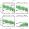 |
Fig. 6. Same as in Fig. 5 for the i filter of Rubin. |
| In the text | |
|
Fig. 7. Ten-year detection distribution as a function of redshift for the eight different networks using the fiducial population (α = 1) with BLh EOS and uniform mass distribution. |
| In the text | |
|
Fig. 8. Ten-year detection distribution as a function of redshift for the reference ET-triangle using the fiducial population (α = 1) and comparing different NS mass distributions and EOS models. |
| In the text | |
|
Fig. 9. Number of injected events and events localised better than 100 deg2, 40 deg2, 20 deg2, 10 deg2, and 1 deg2 by the different detector networks considered in this work for the fiducial population (α = 1) obtained assuming the BLh EOS and uniform NS mass distribution. The left plots show the ET-triangle and the right plots ET-2L shape. In Appendix D, we show the same plots for BLh Gaussian NS mass distribution, and APR4 uniform and Gaussian NS mass distribution. |
| In the text | |
|
Fig. 10. Distribution of SNR and relative errors on detector frame chirp mass, ℳc, luminosity distance dL, inclination angle ι, and first component tidal deformability Λ1. These results are obtained for the fiducial population (α = 1.0) and assuming a uniform NS mass distribution with BLh EOS. |
| In the text | |
|
Fig. 11. Cumulative time required and total number of joint detections for Rubin follow up. Left panels: cumulative time necessary to follow up all the events in the Rubin footprint with a sky localisation smaller than Ω90 (indicated in the x-axis) for ET-triangle as a single observatory, and included in a network of current and future GW detectors as indicated in the legend. The horizontal dashed lines indicate the time corresponding to 10%, 50%, and 100% of Rubin's total observational time in 10 years. Right panels: the corresponding number of optical detections by Rubin. Solid lines are for the KN emission, while dashed lines are for the KN+GRB afterglow. All plots refer to the BLh EOS; the top row plots are obtained using the uniform NS mass distribution and the bottom row ones for the Gaussian NS mass distribution. Thick lines represent the fiducial population (α = 1.0) whereas the thin lines represent the pessimistic population (α = 0.5). |
| In the text | |
|
Fig. 12. Efficiency of joint detections and distribution of inclination angles of BNS mergers. Left panels: efficiency of joint detections as a function of redshift for ET-Δ in each network configuration for both KN (hashed) and KN+GRB (solid) histograms. Right panels: distribution of the inclination angle, ι, for each network configuration indicated in the legends of the left panels. The plots show all the detected (GW) events with a sky localisation within Ω90<100 deg2 for ET alone, Ω90<40 deg2 for ET+LVKI and ET+1CE, and Ω90<20 deg2 for ET+2CE (as used for Fig. 11), the events followed-up as within the Rubin footprint (fp), the corresponding KN detections, and the KN+GRB detections. The plots show the results obtained for the BLh EoS and the uniform NS mass distribution using the 1ep strategy. |
| In the text | |
|
Fig. 13. Number of GW and KN detections in the M1−M2 space. The colorbar indicates the number of GW detections with sky localisation Ω90<5 deg2 (left) and the number of corresponding KN detections for the 1ep detection strategy (right) obtained assuming APR4 (top) and BLh (bottom) EOSs, Gaussian NS mass distribution, α = 1.0, and GW network ET-Δ+2 CE. The black dot shows the peak of the Gaussian mass distribution, that is M1=M2 = 1.33 M⊙. |
| In the text | |
|
Fig. 14. Same as Fig. 13 but for the uniform NS mass distribution. The black dot shows the peak of the Gaussian mass distribution, that is M1=M2 = 1.33 M⊙. |
| In the text | |
|
Fig. 15. Cumulative number of GW detections (dashed lines) and corresponding KN counterpart detections by Rubin (solid lines) as a function of the sky localisation for upgrade configurations of the current detectors; LVKI and 3A#. As a comparison, we show ET alone and in a network with LVKI. The top panels refer to ET-Δ, while the bottom panels to ET-2L. The shown results are obtained using the fiducial population, the BLh EOS, both the uniform and Gaussian NS mass distributions, and 1ep strategy. |
| In the text | |
|
Fig. 16. Parameter estimation capability of different GW detectors (ET alone, LVKI, 3A#, ET+LVKI) in terms of relative error in the luminosity distance (ΔdL/dL) corresponding to the GW detections of Figure 15. The top panels refer to ET-Δ, while the bottom panels to ET-2L. Each curve represents a different GW detector network, and the y-axis shows the cumulative number of GW detections with a relative uncertainty on dL smaller than the values in the x-axis. The maximum Ω90 used in the analysis is set at 100 deg2 for each GW network, except for ET+LVKI for which it is set at 40 deg2. The shown results are obtained using the fiducial population, the BLh EOS, both the uniform and Gaussian NS mass distributions, and 1ep strategy. |
| In the text | |
|
Fig. 17. Cumulative number of KN and KN+GRB counterpart detections obtained as a function of the redshift for ET for both ET-triangle and 2L. The thick lines indicate the 1200 s exposure strategy and the thin lines the 600 s exposure. The detections were obtained following up all the events with a sky localisation smaller than 100 deg2 for ET alone (top panels), 20 deg2 for ET+LVKI (middle panels) and 5 deg2 for ET+1CE (bottom panels). The left panels show the results obtained for the uniform NS mass distribution, while the right panels show the ones obtained for the NS Gaussian distribution. All plots refer to the BLh EOS. |
| In the text | |
|
Fig. A.1. Distribution of NS masses and tidal deformability defined in Eq. (3) (top) and BNS chirp masses and mass ratios (bottom) corresponding to the population with α = 1.0 and Gaussian mass distribution, for APR4 and BLh EOSs. |
| In the text | |
|
Fig. A.2. Distribution of NS masses and tidal deformability defined in Eq. (3) (top) and BNS chirp masses and mass ratios (bottom) corresponding to the population with α = 1.0 and uniform mass distribution, for APR4 and BLh EOSs. |
| In the text | |
|
Fig. B.1. Sensitivity curves used in the analysis. The ET strain noise is plotted considering a single nested detector, composed of a low-frequency and a high-frequency interferometer. Our analysis takes into account that the triangular-shaped ET consists of three nested detectors, each of them with the same sensitivity curve. |
| In the text | |
|
Fig. C.1. Mass of the dynamical ejecta (top), velocity of the dynamical ejecta (centre), and mass of the disc (bottom), as defined in Eq. (6)-(8) for the EOS APR4. x and y axes represent the BNS masses M1, M2. The solid and the dashed black lines mark the chirp mass of GW170817 and GW190425, respectively. The triangular markers show the prompt-collapse mass threshold MPC. |
| In the text | |
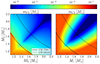 |
Fig. C.2. Same as Fig. 3 but for the APR4 EOS. |
| In the text | |
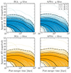 |
Fig. C.3. Same as in Fig. 4 in the case of uniform NS mass distribution. |
| In the text | |
|
Fig. C.4. KNe light curves for BLh (blue lines) and APR4 (red lines) EOSs computed in the g and i filter of Rubin at inclination angle 20 deg, assuming luminosity distance dL = 100 Mpc. KNe light curves correspond to three different BNS systems. Solid lines correspond to M1=M2 = 1.33 M⊙ (the peak of the NS mass distribution); dashed lines correspond to M1 = 1.18 M⊙, M2 = 1.10 M⊙ (the BNS producing the most massive disc); dotted lines correspond to M1=M2 = 1.57 M⊙ (the BNS producing the lightest disc). KNe light curves are compared to AT2017gfo (black diamonds) (Villar 2017) placed at dL = 100 Mpc. |
| In the text | |
|
Fig. C.5. Comparison between AT2017gfo data (apparent AB magnitude) in the B, g, r, i, z, Ks bands (diamonds) (Villar 2017) and the KN light curves corresponding to the brightest and the faintest KN signals obtained by selecting (BNSs) with chirp mass Mchirp = 1.186±0.005 and binary mass ratio q>0.725 from the population with α = 1.0 and Gaussian mass distribution. Dashed and solid lines correspond to the case of APR4 and BLh, respectively. |
| In the text | |
|
Fig. D.1. Ten-year detection distribution as a function of redshift for the eight different networks using the fiducial population (α = 1.0) with BLh EOS and Gaussian mass distribution. |
| In the text | |
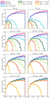 |
Fig. D.2. Same as Fig. 9 in the case of the BLh EOS and Gaussian NS mass distribution. |
| In the text | |
 |
Fig. D.3. Same as Fig. 9 in the case of the APR4 EOS and uniform NS mass distribution. |
| In the text | |
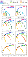 |
Fig. D.4. Same as Fig. 9 in the case of the APR4 EOS and Gaussian NS mass distribution. |
| In the text | |
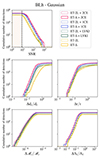 |
Fig. D.5. Same as Fig. 10 for Gaussian mass distribution and BLh EOS. |
| In the text | |
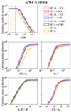 |
Fig. D.6. Same as Fig. 10 for uniform mass distribution and APR4 EOS. |
| In the text | |
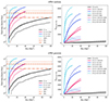 |
Fig. E.1. Same as Fig. 11 for the APR4 EOS. |
| In the text | |
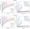 |
Fig. E.2. Same as Fig. 11 for the 2L-shape ET. |
| In the text | |
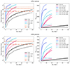 |
Fig. E.3. Same as Fig. 11 for the APR4 EOS and 2L-shape ET. |
| In the text | |
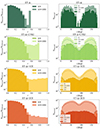 |
Fig. E.4. Same as Fig. 12 but for the Gaussian NS mass distribution. |
| In the text | |
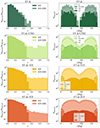 |
Fig. E.5. Same as Fig. 12 but for the APR4 EOS. |
| In the text | |
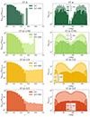 |
Fig. E.6. Same as Fig. 12 but for the APR4 EOS and Gaussian NS mass distribution. |
| In the text | |
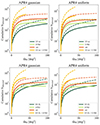 |
Fig. E.7. Same as Fig. 15 but for the APR4 EOS. |
| In the text | |
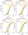 |
Fig. E.8. Same as Fig. 16 but for the APR4 EOS. |
| In the text | |
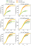 |
Fig. E.9. Same as Fig. 17 but for the APR4 EOS. |
| In the text | |
Current usage metrics show cumulative count of Article Views (full-text article views including HTML views, PDF and ePub downloads, according to the available data) and Abstracts Views on Vision4Press platform.
Data correspond to usage on the plateform after 2015. The current usage metrics is available 48-96 hours after online publication and is updated daily on week days.
Initial download of the metrics may take a while.