| Issue |
A&A
Volume 678, October 2023
|
|
|---|---|---|
| Article Number | A126 | |
| Number of page(s) | 26 | |
| Section | Extragalactic astronomy | |
| DOI | https://doi.org/10.1051/0004-6361/202345850 | |
| Published online | 13 October 2023 | |
Pre-merger alert to detect prompt emission in very-high-energy gamma-rays from binary neutron star mergers: Einstein Telescope and Cherenkov Telescope Array synergy
1
Gran Sasso Science Institute, Viale F. Crispi 7, 67100 L’Aquila, (AQ), Italy
e-mail: This email address is being protected from spambots. You need JavaScript enabled to view it.
; This email address is being protected from spambots. You need JavaScript enabled to view it.
; This email address is being protected from spambots. You need JavaScript enabled to view it.
2
INFN – Laboratori Nazionali del Gran Sasso, 67100 L’Aquila, (AQ), Italy
3
INAF – Osservatorio Astronomico d’Abruzzo, Via M. Maggini snc, 64100 Teramo, Italy
4
Dublin Institute for Advanced Studies, 31 Fitzwilliam Place, D04 C932 Dublin 2, Ireland
5
Max-Planck-Institut fur Kernphysik, PO Box 103980, 69029 Heidelberg, Germany
6
Dipartimento di Fisica e Astronomia ‘G. Galilei’, Università degli studi di Padova, Vicolo dell’Osservatorio 3, 35122 Padova, Italy
7
INFN – Sezione di Padova, Via Marzolo 8, 35131 Padova, Italy
Received:
5
January
2023
Accepted:
5
June
2023
Abstract
The current generation of very-high-energy gamma-ray (VHE; E > 30 GeV) detectors (MAGIC and H.E.S.S.) have recently demonstrated the ability to detect the afterglow emission of gamma-ray bursts (GRBs). However, the GRB prompt emission, typically observed in the 10 keV–10 MeV band, is still undetected at higher energies. Here, we investigate the perspectives of multi-messenger observations to detect the earliest VHE emission from short GRBs. Considering binary neutron star mergers as progenitors of short GRBs, we evaluate the joint detection efficiency of the Cherenkov Telescope Array (CTA) observing in synergy with the third generation of gravitational-wave detectors, such as the Einstein Telescope (ET) and Cosmic Explorer (CE). In particular, we evaluate the expected capabilities to detect and localize gravitational-wave events in the inspiral phase and to provide an early warning alert able to drive the VHE search. We compute the amount of possible joint detections by considering several observational strategies, and demonstrate that the sensitivity of CTA make the detection of the VHE emission possible even if it is several orders fainter than that observed at 10 keV–10 MeV. We discuss the results in terms of possible scenarios of the production of VHE photons from binary neutron star mergers.
Key words: astroparticle physics / gravitational waves / methods: observational / relativistic processes / binaries: general / gamma rays: general
© The Authors 2023
 Open Access article, published by EDP Sciences, under the terms of the Creative Commons Attribution License (https://creativecommons.org/licenses/by/4.0), which permits unrestricted use, distribution, and reproduction in any medium, provided the original work is properly cited.
This article is published in open access under the Subscribe to Open model. This email address is being protected from spambots. You need JavaScript enabled to view it. to support open access publication.
1. Introduction
Gamma-ray bursts (GRBs) are extremely luminous events (∼1052 erg s−1) occurring at cosmological distances. The emission in the prompt phase ranges from milliseconds to several minutes in the keV–MeV range (Kouveliotou et al. 1993). The following multi-wavelength afterglow emission lasts from minutes to months and is observed from radio to very-high-energy gamma rays (VHE; E > 30 GeV). While the afterglow emission is interpreted as deceleration of the GRB jet in the circumburst medium (Paczynski & Rhoads 1993; Mészáros & Rees 1997; Sari et al. 1998), the prompt emission is thought to originate from the internal dissipation of the ultra-relativistic jet either via shocks (Narayan et al. 1992; Rees & Meszaros 1994) or magnetic re-connection (Drenkhahn 2002; Lyutikov & Blandford 2003; Zhang & Yan 2011). Given the unknown origin of the observed GRB spectra, it is not yet clear if GRB jets are primarily baryonic or magnetic in nature (see Piran 2004; Kumar & Zhang 2015; Zhang 2018). Some authors support the scenario in which GRB jets are dominated by kinetic energy (Paczynski 1986; Goodman 1986; Shemi & Piran 1990; Meszaros & Rees 1992; Rees & Meszaros 1992; Levinson & Eichler 1993), and thus the prompt emission is produced either below the photosphere via radiation-dominated shocks (Eichler & Levinson 2000; Ghirlanda et al. 2003; Ryde 2005; Pe’er et al. 2006; Giannios 2012; Beloborodov 2013) or above via optically thin shocks driven by the magnetic turbulence (Narayan et al. 1992; Rees & Meszaros 1994). Others suggest that GRB jets are dominated by the Poynting flux (Usov 1992; Thompson 1994; Mészáros & Rees 1997), and are thus dissipated via magnetic re-connection (Drenkhahn 2002; Lyutikov & Blandford 2003; Zhang & Yan 2011). In most of the scenarios, excluding the sub-photospheric models, the synchrotron radiation from the nonthermal population of electrons (or protons Ghisellini et al. 2020, but also see Florou et al. 2021) is thought to make most of the observed 10 keV–10 MeV emission (Rees & Meszaros 1994; Sari et al. 1996; Tavani 1996). However, the physical parameter space of the source is still unclear (Lloyd & Petrosian 2000; Derishev et al. 2001; Bošnjak et al. 2009; Nakar et al. 2009) given the synchrotron “line of death” problem (Preece et al. 1998; Ghisellini et al. 2000). The reshaped spectra of the synchrotron self-Compton (SSC) component (Papathanassiou & Meszaros 1996; Sari & Piran 1997; Pilla & Loeb 1998; Ando et al. 2008; Bošnjak et al. 2009) by the pairs (Guetta & Granot 2003; Pe’er & Waxman 2004; Razzaque et al. 2004) and/or the high-energy components produced by the photo-pion interactions (Asano & Inoue 2007; Gupta & Zhang 2007; Asano et al. 2009) are expected to give signatures in the VHE domain during the prompt phase. The intensity of this emission depends on the strength of the magnetic field, the size of the emission region, the bulk Lorentz factor, and the acceleration process (proton vs electron energy gain). Therefore, the detection of (or even upper limits on) the VHE emission during the prompt emission phase is critical to establishing the nature of GRB jets.
The recent detection of the VHE emission from the GRB afterglows by the Major Atmospheric Gamma Imaging Cherenkov Telescope system (MAGIC; Aleksić et al. 2016a,b) and High Energy Stereoscopic System (H.E.S.S1) opened up new possibilities of observing these energetic transients. Thanks to the improvement in the sensitivity and smaller response time of the current generation of Imaging Atmospheric Cherenkov Telescopes (IACTs), we are now able to detect the GRB afterglow emission in the TeV band (E > 1 TeV) by the MAGIC and H.E.S.S. telescopes, respectively, as shown for the GRB 190114C (MAGIC Collaboration 2019) and GRB 180720B Abdalla et al. (2019). The detection of GRB 190829A (H. E. S. S. Collaboration 2021) by the H.E.S.S. Collaboration at energies above 100 GeV shows a similar decay profile for the X-ray and VHE components supporting the same emission nature. There were also attempts to detect the VHE emission from the nearby short GRB 160821B using MAGIC (i.e., Acciari et al. 2021). However, the detection significance is below 4σ despite the shortest slew time of 24 s achieved by the MAGIC telescope with respect to any other ground-based TeV instruments to date. The prompt and afterglow emission in VHE from short GRBs have been recently searched by analyzing the High Altitude Water Cherenkov telescope (HAWC) observations. However, looking at the data within 20 s from the burst of 47 short GRBs detected by the Fermi, Swift, and Konus satellites and lying in the HAWC field of view, no detection was found in the energy range of 80–800 GeV (Lennarz & Taboada 2015).
It is noteworthy that for the GRB 221009A (the highest fluence GRB ever detected) the Fermi Large Area Telescope (LAT) detected a high-energy counterpart starting about 200 s after the Fermi/GBM trigger time, and Large High Altitude Air Shower Observatory (LHAASO) reported the detection of several thousand VHE photons up to 10 TeV and beyond within 2000 s of the trigger time (Yong et al. 2022). The LHAASO experiment shows a significant improvement over the present generation (e.g., HAWC) of water Cherenkov detectors with the help of two primary components: the water Cherenkov detector (WCDA), operating in the energy range of 0.3–10 TeV, and the KM2A array, sensitive to energies above 10 TeV. LHAASO (Cao et al. 2019, and references therein), which covers more than 18% of the sky with an almost full duty cycle, is a promising facility to detect the emission from short GRBs in survey mode if the VHE emission peaks above 1 TeV.
The detection of the short and faint gamma-ray burst GRB 170817A (Abbott et al. 2017a; Goldstein et al. 2017; Savchenko et al. 2017) associated with the first gravitational-wave (GW) signal GW170817 observed by the Advanced LIGO (LIGO Scientific Collaboration 2015) and Virgo (Virgo Collaboration 2015) detectors from a binary neutron star merger (Abbott et al. 2017b) marked the beginning of a new era of multi-messenger astronomy including GWs (Abbott et al. 2017c). The multi-wavelength observations from the first seconds to several months after the merger have shed light on the origin of short GRBs as products of binary neutron star (BNS) mergers and on the properties of relativistic jets in GRBs (Abbott et al. 2017c; Hallinan et al. 2017; Troja et al. 2017; Lyman et al. 2018; Alexander et al. 2018; Mooley et al. 2018; Ghirlanda et al. 2019).
Despite the search by MAGIC, H.E.S.S., and HAWC starting a few hours to several days after the BNS merger, no VHE counterpart was detected for GW170817 (Salafia et al. 2021; Abdalla et al. 2017, 2020; Galvan-Gamez et al. 2020). Other GW signals have been followed up by VHE instruments, but without a successful detection to date (Miceli et al. 2019; Seglar-Arroyo et al. 2019a). This is mainly due to the difficulties of searching over the large sky-localization of the GW signals, the slow response time (which is a combination of alert time, observatory slew time, and time required to scan the GW sky-localization), and the limited volume of the Universe observed by the GW instrument. The present-generation IACTs are, in principle, capable of following up the alerts from GW events (Miceli et al. 2019; Seglar-Arroyo et al. 2019a). However, the sky-localization of the GW events are around an order of magnitude larger or more (Abbott et al. 2020) than their field of view (FoV); the FoV of MAGIC (Aleksić et al. 2016a) and H.E.S.S.2 are around 3.5° and 5°, respectively. The VHE is a beamed emission, and only an observer aligned with the jet is expected to observe it. Within the volume of the Universe currently observed by LIGO, Virgo, and KAGRA, the probability of detecting face-on mergers (systems with the orbital plane perpendicular or partially perpendicular to the line of sight) is quite low (see, e.g., Colombo et al. 2022; Patricelli et al. 2022b; Perna et al. 2022).
The next generation of VHE observatories will make it possible to access a larger Universe. They represent a significant and valuable advancement in the search for GW counterparts thanks to the better sensitivity, its ability to monitor large sky-regions, and the rapid response and slew time. The Cherenkov Telescope Array (CTA3) will be capable of observing GRB candidates with unprecedented sensitivity (Cherenkov Telescope Array Consortium 2019). The northern site of the CTA, CTA-N, will consist of the Large-Sized Telescopes (LSTs; López-Coto et al. 2021) and Medium-Sized Telescopes (MSTs; Pühlhofer 2017). The southern site will be equipped with MSTs and the Small-Sized Telescopes (SSTs; Montaruli et al. 2015) with the possibility that two more LSTs will be added. The LST and MST array will be able to cover FoVs up to 50 deg2. In addition, implementation of the divergent pointing (Gérard 2015; Donini et al. 2019; Miceli & Nava 2022), which consists in each telescope pointing to a position on the sky that is slightly offset, in the outward direction, from the center of the FoV, can lead to an ever larger FoV of at least 100 deg2. The SST array is capable of covering a FoV larger than 50 deg2, but it is sensitive to a lower energy range which starts at 1 TeV and begins to perform better only above 5 TeV.
Other works investigate the perspectives to detect the VHE afterglow expected from short GRBs and GW signals associated with BNS mergers detected by the current GW detectors (Patricelli et al. 2022a, 2018; Seglar-Arroyo et al. 2019b; Bartos et al. 2019; Stamerra et al. 2021). In this paper, we evaluate the perspectives to detect the earliest VHE counterpart proposing optimal observational strategies to detect this emission with the next-generation observatories. In particular, we evaluate the joint detection capabilities of CTA working in synergy with the next generation of GW detectors, such as the Einstein Telescope (ET; Punturo 2010; Maggiore et al. 2020) and the Cosmic Explorer (CE; Abbott et al. 2017d; Reitze et al. 2019; Evans et al. 2021). It has been recently discussed and demonstrated that it is possible to detect BNS during the inspiral phase before the merger and to send early warning alerts (see, e.g., Cannon et al. 2012; Sachdev et al. 2020; Magee et al. 2021). The next-generation GW detectors will greatly improve the sensitivity at lower frequencies, also making it possible to have good sky-localizations minutes before the merger (Nitz & Dal Canton 2021; Chan et al. 2018). This translates into providing alerts to the VHE observatory, with an estimate of the localization of the source, in time to slew the VHE instrument to the source and enable a unique opportunity to infer the physics of prompt emission of GRBs. To assess the prospects for joint detection by exploiting the use of early warning alerts of GW events detected before the BNS mergers, we developed an end-to-end simulation that, starting with an astrophysically motivated population of BNS mergers and modeling their GW emission, evaluates the detection and sky-localization capabilities at different pre-merger times for ET working as a single observatory or in a network of observatories including the current and the next generation of GW detectors. We then estimate the number of possible joint GW–VHE detections using CTA. Since the facilities such as LHAASO and SGWO (La Mura et al. 2020) are not pointing instruments (a constant fraction of the sky is always visible), pre-merger alerts do not potentially make improvements for the observation of the VHE counterpart of the GW events.
The paper is organized as follows. Section 2 describes the formalism and methodology for estimating the detection rate of GW/VHE. It starts with a description of the method to evaluate the detection rate and sky-localization of pre-merger GW signals from the population of BNSs observed by ET as a single observatory or by ET included in several GW detector networks. We then describe the capabilities of the CTA array to detect the VHE emission of short GRBs and the observational strategies to detect the earliest emission of BNS mergers. Section 3 describes the results for different observational strategies. Section 4 discusses the plausible emission models capable of producing the VHE signal from short GRBs. Finally, in Sect. 5 we present our conclusions.
2. Methodology to estimate the joint GW–VHE detections
2.1. Population of binary neutron stars
We generate a population of merging BNSs considering systems formed from isolated binary star evolution via a common envelope, as described in Santoliquido et al. (2021). The cosmic merger rate density is built using the semi-analytic code COSMOℛATE4 (Santoliquido et al. 2020), which combines catalogs of isolated compact binaries obtained using the population-synthesis code MOBSE5 (Mapelli et al. 2017; Giacobbo et al. 2018; Giacobbo & Mapelli 2018) with data-driven models of star formation rate (SFR) density and metallicity evolution. Here, we adopt the SFR and average metallicity evolution of the Universe from Madau & Fragos (2017), and a metallicity spread σZ = 0.3. We describe electron-capture supernovae as in Giacobbo & Mapelli (2019), and assume the delayed supernova model (Fryer et al. 2012) to decide whether a core-collapse supernova produces a black hole or a neutron star. When a neutron star forms from either a core-collapse or an electron-capture supernova, we randomly draw its mass according to a uniform distribution between 1 and 2.5 M⊙. This mass distribution is consistent with the GW observations showing broad and flat mass distribution for NSs in binaries (Abbott et al. 2023). Our catalog of synthetic BNS mergers is based on a fiducial scenario that adopts a common envelope ejection efficiency parameter, αCE, equal to 3. We model natal kicks as
 (1)
(1)
where fH05 is a random number extracted from a Maxwellian distribution with one-dimensional root mean square σkick = 265 km s−1, mrem is the mass of the compact remnant (neutron star or black hole), mej is the mass of the ejecta, while ⟨mNS⟩ is the average neutron star (NS) mass, and ⟨mej⟩ is the average mass of the ejecta associated with the formation of a NS of mass ⟨mNS⟩ from single stellar evolution. This kick model, introduced by Giacobbo & Mapelli (2020), is able to match both the proper motions of young pulsars in the Milky Way (Hobbs et al. 2005) and the BNS merger rate density estimated from the LIGO–Virgo collaboration (Abbott et al. 2023). The local astrophysical merger rate of our fiducial scenario is 365 Gpc−3 yr−1, which is consistent with the astrophysical rates inferred from studying the population of compact binary mergers detected during the first, second, and third run of observations of LIGO and Virgo and corresponding to different mass distribution models (Abbott et al. 2023). The union of 90% credible intervals for the different models in Abbott et al. (2023) gives a BNS merger rate between 10 and 1700 Gpc−3 yr−1. As shown in Santoliquido et al. (2021), the common envelope efficiency determines one of the main uncertainties for the number of BNS mergers per year, with larger values of αCE translating into higher merger BNS efficiency. In order to evaluate the impact of the uncertainties of the BNS merger rate normalization on our results, we built two other catalogs of synthetic BNS mergers assuming αCE equal to 0.5 and 5. Throughout the paper, we call the BNS catalog obtained with αCE = 0.5 and αCE = 5 the pessimistic and optimistic scenario catalog, respectively. As shown in Fig. 1 the local merger rates of these populations are still consistent with the range constrained by the LIGO and Virgo observations.
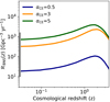 |
Fig. 1. Evolution of the merger rate density in the comoving frame as a function of redshift for the BNS populations used in the present work. Our fiducial population is obtained with a common envelope efficiency αCE = 3 and is represented by the orange solid line. The pessimistic and optimistic populations are obtained with αCE = 0.5 and 5 and are shown by blue and green solid lines, respectively. The grey area shows the 90% credible interval of the local merger rate density, as inferred from the first three observing runs of LIGO, Virgo, and KAGRA (Abbott et al. 2023). |
We consider nonspinning systems, as the NS spin is expected to be small in compact binaries that will merge within a Hubble time, as observed through the electromagnetic channel (Burgay et al. 2003). We generate an isotropic distribution in the sky and a random inclination of the orbital plane with respect to the line of sight.
2.2. GW signal detection and parameter estimation
The next-generation detectors aim to make the low-frequency band below 10 Hz accessible. ET will be built underground, and it is expected to cover frequencies down to 2 Hz. Extending observations at low frequencies increases the in-band duration of BNS signals, offering two key advantages for the successful detection of prompt electromagnetic counterparts: to accumulate a high enough signal-to-noise ratio (S/N) before the merger to make pre-merger detection and early warning possible and to significantly improve the sky-localization accuracy by using the imprint on the signal amplitude of the time variation of the detector’s response due to the daily rotation of Earth.
In order to evaluate the pre-merger detection and sky-localization capability for ET as a single observatory or included in a network of detectors, we use the Fisher-matrix approach implemented in GWFish (Dupletsa et al. 2023)6. The code estimates the uncertainties on the measured source parameters from simulated GW observations, taking into account the effects of the time-dependent detector response and the Earth’s rotation on long-duration signals, such as those from BNS coalescences.
We built a simulation injecting a GW signal for each BNS merger of the population described in Sect. 2.1 up to redshift z = 1.5. This redshift is conservatively larger than the maximum distance up to which CTA will be able to detect the VHE prompt emission expected for short GRBs. We inject 2.7 × 10⁵ BNS signals, corresponding to the number of BNS mergers up to redshift z = 1.5 that we can observe at Earth in one year with a perfect detector, according to our fiducial scenario. For the pessimistic and optimistic scenarios, we inject 2.0 × 10⁴ and 4.0 × 10⁵, respectively. The inspiral GW signal for each merging BNS is constructed using a post-Newtonian formalism, in particular the TaylorF2 waveforms (Buonanno et al. 2009). The S/N is computed by GWFish during the inspiral, applying a high-frequency cutoff at four times the frequency of the innermost stable circular orbit (see Dupletsa et al. 2023, for details). A network S/N higher than 8 is used to select each BNS detection.
We consider five GW detector configurations: ET as a single triangular 10 km arm-length detector located in Sardinia (one of the possible European site candidates to host ET); ET plus a network of five second-generation detectors; ET plus two Voyager detectors (located in the current USA LIGO sites); ET plus CE (L-shaped 40 km arm-length detector located in the USA); and ET plus two CEs (one located in the USA and one in Australia). For the second-generation network, we consider Advanced LIGO, Virgo, and KAGRA with the optimal sensitivity (phase plus) expected for the fifth run of observations, as in Abbott et al. (2020), and the same version of the LIGO detector in India. For ET we use the ET-D sensitivity curve (Hild et al. 2011). For Voyager and CE(40 km), the sensitivity given in Adhikari et al. (2020) and Evans et al. (2021), respectively. For each GW detector and for each of the three combinations of high- and low-frequency interferometers of ET, we assume a duty cycle of 85% (Branchesi et al. 2023).
We evaluated the sky-localization and other parameters of the detected sources 15, 5, and 1 min before the merger and at the merger time for the different detector configurations. These pre-merger times are appropriate, both to select events with a suitable pre-merger sky-localization to be observed by the CTA and to have adequate time for the CTA to respond to the trigger, to point and observe the sky-localization to detect the VHE emission (see Sect. 2.3). We then focus on face-on events (the orbital plane perpendicular, assumed to be aligned with the jet, within 10 degrees with respect to the line of sight). These are the events for which we expect to detect the VHE counterpart.
Our analysis is based on the assumption of a Gaussian noise background in the GW detectors. In a more realistic scenario, other backgrounds need to be accounted for: (1) a stochastic GW background of unresolved compact binaries that might affect ET analyses below 20 Hz, (2) an overlap between individual resolvable signals and its potential impact on signal analyses, and (3) instrumental noise transients (glitches). The nonstationary stochastic GW background might reduce the S/N of GW observations at times (on average, it is weaker than instrument noise). However, the triangular configuration of ET makes it possible to assess the impact of the GW background and mitigate it (Goncharov et al. 2022). A recent study suggests that the overlap between individual resolvable signals will not have an important effect on signal analyses (Samajdar et al. 2021). Instrument glitches can in principle affect signal analyses, but effective glitch mitigation methods are under development, and we can assume that optimized signal plus noise Bayesian analyses will be available when ET starts operation (e.g., Chatziioannou et al. 2021).
2.3. CTA array specification and observational strategies
CTA is expected to increase our capabilities to perform a follow-up and detect transient events (Cherenkov Telescope Array Consortium 2019) thanks to the unprecedented sensitivity, field of view, and rapid slew to any given direction. During the first construction phase, the approved configuration is called α-configuration7. This configuration will consist of 14 MSTs and 37 SSTs in the southern site at the Paranal Observatory (Chile). The northern site at the Roque de los Muchachos Observatory (Spain) is expected to host LSTs and nine MSTs. The specification of the different telescopes sizes within the alpha-configuration are given in Table 1. LSTs, MSTs, and SSTs are designed to cover different science cases. The array of SSTs has the largest sky coverage (> 50 deg2), whereas the array of four LSTs has the smallest sky coverage (∼13 deg2). While the SST array effectively covers events with energies from 5 to 300 TeV, the LST and MST arrays target lower energy events from 20 and 150 GeV, respectively. Partial CTA operation has recently started with one LST in the northern site (López-Coto et al. 2021), covering the energy band of 10 GeV to 10 TeV.
Detector specification of CTA (α-configuration) as compared to the current-generation IACT (i.e., MAGIC).
Building the optimal CTA follow-up of GW signals from BNS mergers requires taking into account duration, luminosity, energy band of the expected VHE counterpart combined with slewing time (tslew), field of view (FoV), and sensitivity of CTA. Since the expected energy band for the VHE counterparts of GW events is sub-TeV, we consider the use of LSTs and MSTs in the present work, excluding SSTs from the analysis. Although the SST array is expected to have larger sky coverage, it does not cover the energy band below 1 TeV. CTA is expected to operate in a hybrid mode with LST and MST (individual sub-arrays) observing together or separately (Actis et al. 2011; Cherenkov Telescope Array Consortium 2019). In this work we consider separately the individual components of CTA (LSTs and MSTs) in order to increase the effectiveness of operation taking into account the different slewing times. We assume a FoV of 10 deg2 and slewing time (tslew) of 20 s for the LST sub-array. Although the southern LST is not yet guaranteed, we consider LSTs located in the northern and the southern hemispheres. The MST sub-array (one located in the northern and one in the southern hemispheres) is assumed to have a FoV of 30 deg2 and slewing time (tslew) of 90 s. Our assumption of a smaller FoV, compared to the design FoV, for both LST and MST sub-arrays accounts for the reduction in the angular resolution and energy reconstruction capability for the off-axis events (Cherenkov Telescope Array Consortium 2019). We consider a duty cycle of 15%. We also assume a 50% reduction on the sky visibility taking into account that the sub-arrays are hardly capable of observing the sky above the zenith angle of 60°.
We then explore three observational strategies to follow up the events triggered by the GW network:
-
direct pointing of events, which uses sky-localization smaller than the FoV to detect the prompt emission;
-
one-shot observation strategy, which consists of following up triggers using a single observation randomly located in the sky-localization uncertainty of the GW signal to detect the prompt emission, and possibily also using divergent pointing (see Sect. 3.2.3);
-
mosaic strategy, which tiles the sky-localization being more effective to detect the afterglow emission.
For each event, we consider the total time to be spent consisting of time to respond to the trigger (talert), slewing time (tslew), and exposure time (texp). In order to detect the prompt emission, we consider a single exposure of 20 s starting around the merger time. This exposure is longer than the delay of a few seconds expected between the GW and the prompt gamma-ray emission of short GRBs (Zhang 2019), but enables the detection of possible VHE emission with a larger delay without preventing the detection of a signal with smaller latency. During the post-processing of the observed data, the signal can be extracted by analyzing a shorter exposure (e.g., 2 s). This exposure allows us to sample isotropic energy of 1050 erg in the 0.2–1 TeV up to redshift of 1 (see Sect. 2.4) and to follow up several GW triggers. In order to reach the source location before the merger takes place and capture the prompt emission, we consider pre-merger alerts. The response time and slewing time can in principle be reduced to 1 min (talert + tslew) for the LST sub-array, thanks to its rapid slewing time of 20 s. Thus, in a very optimistic scenario, the LST sub-array can follow up (even) one-minute pre-merger alerts and reach the source location at the merger time. Instead, due to a longer slewing time for MST of about 90 s, a longer pre-merger time is required for detecting the prompt emission. A minimum pre-merger alert time of five minutes is considered for MST in our study. More details on the observational strategies and time required to follow up GW events are given in Sect. 3.2. The sketch of the proposed observational scheme is shown in Fig. 2.
 |
Fig. 2. General observation scheme for detection of the VHE prompt emission phase of the BNS merger. The low-frequency observations made possible by the next generation of GW detectors will enable an inspiraling BNS system to be detected and localized before the merger. A pre-merger alert for the event is sent and the VHE detectors can rapidly point to the target during the merger. The delay between the GW and VHE emission is assumed to be within our exposure time of 20 s. |
2.4. Detection of GRBs in VHE band by IACTs
To evaluate the isotropic energy from short GRBs sampled by CTA as a function of the redshift, we assume an intrinsic spectrum of the VHE emission of the form
 (2)
(2)
where Γ is the spectral index, E0 is the energy scale, and Ec represents the intrinsic cutoff energy.
The observed spectrum is evaluated as follows
 (3)
(3)
where the normalization N0 is given by
![Mathematical equation: $$ \begin{aligned} {N_{0}(E)}= \frac{E_{\rm ISO}\times (1+z)}{ 4 \pi d^2_L {\int ^{E_2/(1+z)} _{E_1/(1+z)}} ~\mathrm{d}E ~E ~\mathrm{exp}[-\tau (E,z)] \left(\frac{E}{E_0}\right)^{\Gamma } exp(-E_c) }. \end{aligned} $$](/articles/aa/full_html/2023/10/aa45850-23/aa45850-23-eq5.gif) (4)
(4)
Here exp[−τ(E,z)] is the extragalactic background light (EBL) correction factor (Domínguez et al. 2011), EISO is the isotropic energy in the VHE gamma-ray band (0.2–1 TeV) for a duration of the burst of 10 s, and z the redshift of the source.
We simulate a number of GRB spectra varying the isotropic energy (EISO) in the range [1042–1053 erg] and redshift in the range [0.001–1.5] for three levels of cutoff energy Ec: 100 GeV, and 1 TeV. The cutoff is assumed for the indices −1.5 and 2.0. We also consider two cases, Γ = −2.0 (similar to the VHE afterglow detected by MAGIC for GRB 190114C; MAGIC Collaboration 2019) and Γ = −3.0 without assuming any intrinsic cutoff. Figure 3 shows the intrinsic and observed spectra for several spectral indices and the cutoff energies for a source at z = 0.1.
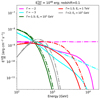 |
Fig. 3. Intrinsic (assumed) and observed spectra for VHE transient events with specific spectral indices (Γ) and cutoff (Ec) for the isotropic energy |

Using the observed spectra, we estimate the number of excess events Nex and the significance of detection (σ) from the MAGIC performance paper (Aleksić et al. 2016a). The significance of detection (σ) is obtained using the Li & Ma method (Li & Ma 1983) for all the grid points [EISO, z]. We consider the simulated GRB as detected when σ > 5 and Nex > 10. In order to obtain the detection limit of CTA, we scale the number of excess and background events using the Crab-signal rate observed by MAGIC by the ratio of collection area for specific energy bins. The collection area for MAGIC and CTA are obtained from Aleksić et al. (2016a) and CTA webpage8, respectively. The background events for CTA as a function of energy are also obtained from the CTA webpage4, and are later converted into rate [events/ min] by multiplying by the point spread function (PSF) of CTA as a function of energy. Figure 4 shows the detection limit on the isotropic energy ( ) for a VHE emission of 10 s in the range 0.1–1 TeV as a function of redshift considering a detection threshold of σ > 5 and Nex > 10 for several spectral indices and cutoff energies. The detection limit is obtained for the sensitivity of CTA-N (α-configuration including four LSTs operating with nine MSTs).
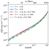 |
Fig. 4. Lower limit on isotropic energy (EISO) in the range 0.2–1 TeV as a function of redshift for CTA-N (α-configuration including four LSTs and nine MSTs). A short constant VHE emission of 10 s is considered, and a threshold is used on the significance (σ) of 5σ and on excess gamma-ray events (Nex) larger than 10 to define a detection. A conservative energy threshold of E > 200 GeV (hence a slightly higher limit on |


The operation of LST as an independent array might increase the detection limit by a factor of 2–3 (Bernlöhr et al. 2013) in the energy band of 0.2–1 TeV. MST is more sensitive than LST in the 0.2–1 TeV band and the detection limit does not change significantly with respect to the entire CTA array. As a comparison, we highlight that the afterglow emissions detected by MAGIC for GRB 190114C and by H.E.S.S. for GRB 180720B correspond to isotropic energies of 2 × 1052 erg and 2 × 1054 erg, respectively (MAGIC Collaboration 2019; Abdalla et al. 2019), which are far above our detection limit.
The detection of gamma rays with energy above ∼20 GeV is based on the indirect technique of detecting atmospheric Cherenkov light produced by the VHE photons coming from the astrophysical TeV emitters (point sources or extended sources). The extensive air showers (EAS) produced by hadrons act as a background and might mimic a transient signal. However, there are solid analyses to reject this background that are already implemented in the data analysis technique of current generation detectors (such as MAGIC and H.E.S.S). In the present analysis we take into account the background and rely on the random-forest method used by the MAGIC telescope system (Aleksić et al. 2016a). On the basis of our current VHE observations, the VHE gamma-ray sky is not polluted with the presence of several sources given that they are not in the vicinity of any known extended sources. The astrophysical contaminants that can potentially mimic the VHE counterpart of the GW signals are expected to be removed easily.
3. Results
3.1. Pre-merger detections and sky-localization
The results of the simulations evaluating the detection rate and pre-merger sky-localization are summarized in Tables 2 and 3, where we show ET as a single observatory, and ET included in different networks: ET plus the second-generation detectors LIGO-Livingston, LIGO-Hanford, LIGO-India, Virgo, and KAGRA (ET+LVKI+); ET plus two Voyager in the USA (ET+2VOY); ET plus CE in the USA (ET+CE); ET plus two CEs, one in the USA and one in Australia (ET+2CE). The number of detections per year for a specific threshold of sky-localization (Ω (90% c.l.) = 0.1, 1, 10, 30, 100, and 1000 deg2) is given for three different pre-merger times (15, 5, and 1 min before the merger) and at the merger time. The quoted numbers refer to the fiducial population (αCE = 3). The pessimistic (αCE = 0.5) and optimistic (αCE = 5) scenarios are given in square brackets. Table 3 shows the detections per year of simulated BNS mergers with a viewing angle (θv; the angle between the line of sight and the perpendicular to the orbital plane of the BNS system) smaller than 10°. Since the VHE emission is expected to be beamed along the jet, these events are the ones for which we expect a VHE counterpart to be detectable.
Number of detected (network S/N > 8) BNS mergers per year within z = 1.5 for different GW detector configurations.
The cumulative distribution of detections per year up to redshift equal to 1.5 as a function of the sky-localization is shown in Fig. 5 for the different detector configurations. For 15 and 5 min pre-merger scenarios, the cumulative distributions for ET as a single observatory, ET+LVKI+, and ET+2VOY are the same, indicating that ET is the main observatory that localizes in the network. The presence of second-generation detectors or the two Voyagers improves the sky-localization one minute before the merger, and the improvement becomes largely significant at the merger time. The presence of CE in the network significantly improves the sky-localization capabilities pre-merger of ET also 15 min before the merger. As shown in Fig. 5, when ET is included in a network of next-generation GW detectors, the cumulative number of detections tends to flatten for sky-localizations larger than 1000 deg2 because the network localizes most of the events better than this value (see Fig. 6).
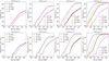 |
Fig. 5. Cumulative number of detections (S/N > 8) per year for different networks of GW detectors considering 15, 5, and 1 min before the merger and at the merger time. The top panels show the detections considering BNS systems with all orientations. The bottom panels show the detections of BNS systems with a viewing angle smaller than 10° (on-axis events), a fraction of which are expected to produce detectable VHE emissions. For each of the simulations, the injected BNSs are within redshift z = 1.5. The quoted detection numbers refer to the fiducial population and are obtained assuming a duty cycle of 0.85 (see text). For the 15 and 5 min pre-merger scenarios, the ET+LVKI+ and ET+2VOY do not show any significant difference with respect to ET as a single observatory (the red and green lines lie under the purple line). |
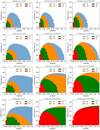 |
Fig. 6. Redshift distribution of sky-localization uncertainty (given as 90% credible region) for three detector configurations: ET, ET+CE, and ET+2CE. The absolute numbers refer to the fiducial BNS population sample and detections within a redshift of 1.5 per year of observation assuming a duty cycle of 0.85 (see text). The panels show the detections and the corresponding sky-localizations as a function of the redshift 15, 5, and 1 min before the merger and at the merger time. The blue histogram (“All”) shows all the detected sources. |
The sky-localization capabilities of ET, ET+CE, and ET+2CE, at five minutes and at one minute before the merger and at the time of the merger are shown in Fig. 6 as a function of redshift for the fiducial population of the BNS (αCE = 3). The number of well-localized events (Ω < 100 deg2) are nonnegligible (on the order of hundred) already five minutes before the merger and up to z = 0.4 for ET as a single observatory. This number increase to thousands of detections up to z = 0.5 for ET+CE and ET+2CE. One minute before the merger several thousands of detections have sky-localizations Ω < 100 deg2 for ET+CE (ET+2CE) up to z = 1.0 (1.3), and hundreds have sky-localizations Ω < 10 deg2 up to z = ∼0.4 for ET+CE and ET+2CE.
Our pre-merger sky-localization results are in agreement with those of Nitz & Dal Canton (2021) and Li et al. (2022). For example, despite the different BNS populations and detection criteria (S/N > 12 and 100% duty cycle), Li et al. (2022) find 7 and 210 events per year for sky-localization of < 1 and 10 deg2 detected by ET+2CE 5 min before the merger. These numbers match those in this study: 𝒪(10) and 𝒪(100). Also in the case of ET alone, 5 min before the merger Nitz & Dal Canton (2021) find 6 and 94 detection per year with sky-localization smaller than 10 and 100 deg2, which is again in agreement with our numbers 𝒪(10) and 𝒪(100), respectively. Li et al. (2022) found several hundred detections with sky-localization smaller than 30 deg2 before the merger for ET+2CE, as in the present work. The number of events detected and localized at the time of the merger are in agreement with the extensive work of Ronchini et al. (2022) and Iacovelli et al. (2022; taking into account that the present work analyzed events up to z = 1.5).
Our follow-up observational strategies for the next generation GW detectors are based on the presence of low-latency pipelines and infrastructure able to detect GW event candidates and send public alerts in almost real time, as currently done by the LIGO, Virgo, and KAGRA collaborations (Abbott et al. 2020, 2019). We assume an alert time (talert) of 30 s covering the time to detect an event, transmit it, and receive the alert. The current low-latency detection pipelines are able to detect an event within 10 s (Chu et al. 2022). They perform a matched-filter search for binary merger signals using a bank of GW template waveforms, and give in low latency a first estimate of the source parameters (including sky-localization and viewing angle). Currently, the latency to send an alert is dominated by the semi-automated detector characterization and data quality checks which bring the detection alert latency to a few minutes, but efforts are ongoing to reduce this time to an order of seconds. We consider a talert = 30 s appropriate for the next generation detector to include possible delay in the transmission and receipt. In the case of data quality check delays similar to the current ones, the only observational strategy whose results could be negatively impacted is that of LST following a 1 min pre-merger alert (the strategy called LST-c in Table 5), which we consider the most risky strategy in our work.
3.2. CTA observational strategies and detectability
The detection of VHE emission from BNS merger is currently challenging because of (a) the large sky-localization of GW signals relative to the FoV of IACTs, (b) the long delay between the merger time and the GW alert time and response time of IACTs, and (c) the small volume of the Universe up to which GW detectors are able to observe BNS mergers, which gives a small probability of detecting on-axis events from which VHE is expected. The study presented in the paper shows that the era of ET and CE can mark a paradigm shift mostly because of the ability to provide pre-merger alerts with a good sky-localization even 15 min before the merger. In addition, the effectiveness of the VHE counterpart search will increase due to the improved sensitivity of the next generation GW detectors, which will increase the number of on-axis event detections, and the large FoV, unprecedented sensitivity, and short slewing time of CTA.
We assume that the prompt VHE emission originating from the processes described in Sect. 4 is short-lived and detectable in an observational window of 20 s around the merger time. We focus on the pre-merger alert scenarios of 15, 5, and 1 min before the merger. We consider an alert time (talert) of 30 s corresponding to the communication of the alert among the GW detector network and CTA, the CTA-LST (-MST) slew time (tslew) of 20 s (90 s), and an exposure time (texp) of 20 s. We also add tadd 10 s, which includes a possible repositioning and the uncertainty on the estimation of the merger time. The total CTA time for one single observation is tobs = tslew + tadd + texp = 50 s and 120 s for LST and MST, respectively.
For the one-minute pre-merger alerts, we only consider the LST array since it has a faster slew time of less than 20 s. However, the chances of detection are reduced by the smaller sky-coverage of LST which has a FoV of around 10 deg2. The slew time of 90 s for MST makes it impossible to follow the one-minute pre-merger alerts. In contrast, the MST array is appropriate for following up the 5 and 15 min pre-merger alerts. Although the number of GW detections to be followed up is smaller than in the case of one-minute pre-merger alerts, the FoV of 30 deg2 is an advantage.
In the following we examine the results for four observational strategies: direct pointing of well-localized events, one-shot observation, divergent pointing, and mosaics.
3.2.1. Direct pointing of well-localized events
We explore the direct pointing strategy by selecting events with sky-localization smaller than 10 and 30 deg2 taking into account the adopted FoV for the LST and MST arrays, respectively. In Table 2 the number of events with sky-localization smaller than 10 deg2 to be followed up by the LST array is around ten per year, one minute before the merger for ET, ET+LVKI+, and ET+2VOY considering the fiducial population. This number increases to around two hundred (more than six hundred) for ET+CE (ET+2CE). Among these events, as shown in Table 3, the number of events on-axis (i.e., the events with a viewing angle smaller than 10° from which we expect to observe the VHE) is negligible for ET, ET+LVKI+, and ET+2VOY, and it becomes on the order of a few (several) tens for ET+CE (ET+2CE).
The number of on-axis events with sky-localization smaller than 30 deg2 five minutes before the merger is negligible for ET, ET+LVKI+, and ET+2VOY. This number becomes a few tens for ET+CE and ET+2CE (see Table 3). These events can be detected in VHE by using the MST array following up a few hundred (several hundred) of 5 min of pre-merger alerts (see Table 2).
To estimate the actual number of joint detections, it is necessary to take into account the CTA duty cycle of 15% and the CTA visibility. Considering that CTA telescopes are able to observe sources with an elevation larger than 30 deg, this reduces the visible sky by a factor of 2. Another factor to consider is the fraction of BNSs that produce a jet. Although this fraction is still largely uncertain, studies combining electromagnetic observations of short GRBs and BNS merger rates from GW observations indicate that a 20 − 50% fraction of BNS mergers produce a jet (e.g., Ronchini et al. 2022; Colombo et al. 2022; Salafia et al. 2022). Considering all these factors, the direct pointing strategy is expected to give a few joint detections per year only when ET operates in a network of three next-generation detectors. No joint detections are expected for the pessimistic BNS population scenario.
3.2.2. One-shot observation strategy
In order to increase the number of events to be followed, we propose a strategy that for each detected event uses a one-shot observation covering an area corresponding to the FoV of CTA-LST and -MST (10 and 30 deg2).
The percentage of CTA total observational time in one year that would be spent following all the individual events by a one-shot observation randomly positioned in the sky-localization area is shown in the central plots (second column) of Fig. 7 for MST and Fig. 8 for LST. This percentage is evaluated as the fraction of CTA observational time necessary to follow up all the events with sky-localization smaller than that indicated on the x-axis
 (5)
(5)
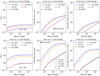 |
Fig. 7. Expected number of detections by CTA-MST using the one-shot observation strategy (left column). The estimates of the number of possible VHE counterparts are based on the on-axis BNS systems (systems injected with θv < 10° in our simulations) and are evaluated as described in the text (see Eq. (6)). These estimates assume that all BNS produce a jet. They take into account the sky-localization (Ωi) of each event, the MST field of view of 30 deg2, the CTA duty cycle of 15%, and the CTA visibility limited to a zenith angle larger than 60° (minimum elevation of 30°). The fraction of CTA time spent following all the GW alerts with the sky-localization smaller than the one indicated on the x-axis is given by the plots in the central column. To observe each event (independent of the sky-localization) the observational time (tobs) is considered, given by the sum of slewing time (tslew = 90 s), an additional re-positioning time (trep = 10 s), and the exposure time (texp = 20 s). The plots in the right column show the CTA time when only triggers with an observed θv < 45° are followed up resulting in a significant reduction of CTA time. |
where N(< Ω) is the number of events with sky-localization smaller than Ω, tobs is the observational CTA time spent for each event, and CTATOT the total observational time of CTA in one year including the duty cycle of 15%. The visibility of CTA, CTAvis = 0.5, takes into account that CTA telescopes are able to observe sources with an elevation larger than 30 deg. The tobs is set to 120 s for MST and 50 s for LST. The observational strategy consists of receiving the pre-merger alert and beginning to slew the telescopes just before the estimated merger time (which we assume is given in the alert). For the MST, we consider only 15 and 5 min pre-merger alerts; after receiving the alert, the MSTs start the slew about 100 s before the merger time. For the LST (thanks to the very rapid slew time of 20 s), we also consider the 1 min pre-merger alerts. In this case, after receiving the alert the LST slewing starts 30 s before the merger time given in the alert.
For the 15 and 5 min alerts, we also consider a double-step strategy. For all the events localized with a sky-localization smaller than 1000 deg2 we initially point the center of the sky-localization uncertainty and then we re-point the antennas based on the updated sky-localization obtained 1 min before the merger which is expected to be significantly smaller. Since the Fisher matrix approach does not give the real shape of the sky-localization uncertainty and the distribution probability within it, we approximate the sky-localization with a circular error region and a uniform distribution probability to contain the GW source within it. Given the angular radius of the LST FoV of about 2°, the maximum required repositioning for an error region of 1000 deg2 (angular radius of 18°) is ∼16°, which corresponds to a repositioning time of about ∼3 s. The required repositioning time for MST (angular radius of 3°) for a movement of 15° is about ∼10 s. We consider the same repositioning time of trep= 10 s for both LST and MST. Our follow-up strategy to detect the prompt VHE emission relies on the precision of the merger time, which is expected to be given in the alert. The uncertainty on the merger time is estimated by the Fisher matrix analysis to be much smaller than 0.1 second for events localized better than 1000 deg2. Tables 4 and 5 summarize the different observational strategies included in the present analysis: (1) following up all the events detected 15 min before the merger (MST-a, LST-a), (2) following up all the events detected 5 min before the merger (MST-b, LST-b), (3) following up all the events detected 1 min before the merger (LST-c), and (4) using the improved sky-localization updated 1 min before the merger (MST-c, MST-d, LST-d, LST-e).
Observational strategies of following up pre-merger alert events with CTA-MST.
Observational strategies of following up pre-merger alert events with CTA-LST.
The central plots of Fig. 7 show the percentage of CTA time necessary to follow up all the events detected by ET alone or in a network of detectors with a one-shot observation of MST. They refer to the fiducial BNS population and the 15 and 5 min pre-merger alerts (MST-a and MST-b strategies in Table 4). Figure 8 shows the same for LST (LST-a and LST-b strategies in Table 5). For LST a plot is added (third row) for the 1 min pre-merger alerts (LST-c strategy in Table 5).
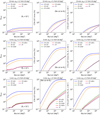 |
Fig. 8. Same as Fig. 7, but considering LSTs. A FoV of ∼10 deg2 is used and the observational time for each event (tobs) of 50 s is given by the slewing time (tslew) of 20 s, an additional repositioning time of 10 s, and the exposure time (texp) of 20 s. Thanks to the rapid slew time for LST, we also consider the scenario where the 1 min pre-merger alerts are directly followed. |
The follow-up with MST of all the events detected 15 min before the merger and with sky-localization smaller than 104 deg2 is possible at the cost of around 4% CTA observational time for ET+2CE and ET+CE, and around 2% for ET alone. The number of detected events 5 min before the merger is larger than those detected 15 min before the merger, and the amount of time to follow up all of them is around 40% and 50% of CTA time for ET+CE and ET+2CE, and 4% of the CTA time for ET alone.
Using LST, the CTA time budget will be exhausted by following up all the events with a pre-merger alert of 1 min and with sky-localization smaller than around 1000 deg2 for ET+2CE and with sky-localization smaller than about 104 deg2 for ET+CE. Only 10% (20%) of CTA-LST time will be consumed following the 5 min pre-merger events with sky-localization smaller than about 103(104)deg2 for ET+CE (ET+2CE). Due to the smaller observational time for each observation of LST, for the 15 min and 5 min alerts, the observational time reduces by about a factor of 2 with respect to MST.
We then estimate the expected number of VHE counterparts detectable with the one-shot observation method. Since the VHE emission is expected only from on-axis events, we identify all the events injected with θv < 10° and detected by the GW detectors in our simulation. Due to the fact that the estimate of θv from the GW data will not be precise enough to directly select on-axis events (see Fig. B.1 for the distribution of the uncertainty on the viewing angle), our observational strategy consists in following up all the GW triggers. The expected number of possible VHE detections per year by observing all the GW triggers is evaluated by summing over all the on-axis events (θv < 10°) with sky-localization smaller than a threshold (Ω)9 and by assigning to each on-axis event a weight based on its sky-localization, FoV/Ωi (its probability to be detected with one-shot observation decreases for larger sky-localization):
 (6)
(6)
For each event with Ωi < FoV, the fraction FoV/Ωi is set equal to 1. D.C. is the CTA duty cycle of 15% and CTAvis the CTA visibility of 50%. While the cumulative distribution of on-axis events Nθv < 10° as a function of sky-localization is shown in the lower panels of Fig. 5, the cumulative distribution of the expected number of possible VHE counterpart detection NVHE as a function of sky-localization for the one-shot observation strategy is given by the plots in the first column of Figs. 7 and 8 for MST and LST, respectively. By looking at these plots together with those of CTA time (second column), it is possible to estimate the expected number of possible VHE detections following all events with a sky-localization below a certain threshold and the corresponding amount of CTA time required.
Following pre-merger alerts of 15 min, we expect to detect around 1 VHE possible counterpart per year by CTA-MST operating with the network of ET and CE (ET+CE and ET+2CE). This number increases to around ten possible VHE counterparts per year for ET+CE (ET+2CE) following pre-merger alerts of 5 min with sky-localization smaller than 103 deg2 by using 25% (40%) of time of CTA-MST operating with ET+CE (ET+2CE).
Using CTA-LST we do not expect detection, even with ET+2CE following all the GW events with 15 min pre-merger alerts. However, we expect around 3 (5) possible detections per year triggered by ET+CE (ET+2CE) using 10% (20%) of the CTA time budget and following all the events with sky-localization of 103 deg2. Around ten possible VHE counterparts are expected by following the 1 min pre-merger alerts with sky-localization smaller than about 200 deg2 detected by ET+CE at the expense of 20% of the CTA time. Twenty possible VHE detections are expected for ET+2CE by following all the events with sky-localization smaller than 102 deg2 detected by ET+CE at the expense of about 10% of the CTA time. Only following pre-merger alerts of 1 min can give a few detections for ET as a single observatory or operating in the network ET+LVKI+ and LVK+2VOY. All these numbers are obtained using the fiducial population and considering all BNS launching a successful jet. However, as written in the previous section, on the basis of the current studies only 20 − 50% are expected to produce a jet.
This research can benefit from the reduction of CTA time to be devoted to the follow-up of events while maintaining the same VHE detection efficiency. For example, the viewing angle is estimated from the GW signals in low latency, and it can be used to remove all the off-axis systems from which the VHE emission is not expected. This makes it possible to reduce the number of events to be followed up by CTA, and thus the CTA time to be spent on this search. Figure B.1 shows the uncertainty on the viewing angle coming from the analysis of the GW observations as a function of injected θv of the BNS system. It can be inferred from the figure that the observed uncertainties on the viewing angles are large and in particular are larger for smaller viewing angles. Therefore, it is not possible to directly select on-axis events (θv < 10°), but based on the smaller errors on larger viewing-angles, it is safer and more effective to exclude off-axis events from the follow-up. We choose an arbitrary threshold on θv = 45° which enables us to exclude a large number of off-axis events and to limit the number of excluded on-axis events. The plots in the right column of Figs. 7 and 8 show the percentage of CTA time to follow all the events with θv < 45°. This selection based on the observed θv reduces the total follow-up time by about a factor of 3. As also shown in Ronchini et al. (2022), to optimize the observational strategy and increase the efficiency of the search in the era of 3G detectors, it will be critical to send information on the source parameters beyond distance and sky-localization which are the only source parameters currently sent in low latency for LIGO, Virgo, and KAGRA event candidates.
We also evaluated the possibility to use updated information on the source parameters; following up the pre-merger alerts of 15 min or 5 min, we use the updated sky-localization available 1 min before the merger (see MST-c and MST-d in Table 4, and LST-d and LST-e in Table 5). For this scenario we consider to follow up only events with sky-localization smaller than 1000 deg2 during the initial alerts. Figure C.1 shows the improvement of the sky-localizations over time from sky-localizations at 15 or 5 min to 1 min. The updated sky-localization at 1 min clusters around 100 deg2 for the cases of ET+CE and ET+2CE for both the 5 and 15 min scenarios. Although this strategy offers a significant improvement, it counts on a very rapid communication and response to the updated alert and a possible rapid repositioning. Any delay in the response or slewing of CTA could be problematic. Figure 9 shows the results for this observational strategy providing the possible VHE detections by MST (left column) and LST (right column).
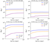 |
Fig. 9. Same as Figs. 7 and 8 following up 15 and 5 min pre-merger alerts, but using the updated sky-localization obtained 1 min before the merger. For this scenario, only events detected 15 min or 5 min before the merger with sky-localization less than 1000 deg2 are considered. The expected number of VHE possible detections includes the CTA visibility because LST and MST antennas are not able to observe below the elevation angle of 30° (zenith higher than 60°). The plots in the right column show the LST array and the plots in the left column the MST array. |
For CTA-MST, the expected number of possible VHE counterparts using updated information on the 1 min pre-merger alert sky-localization are 2.5–3 (20–40) events when alerted by ET+CE and ET+2CE 15 min (5 min) before the merger; these numbers compare to around 1 (10) detections if the 1 min sky-localization update is not used (see plots in the left column of Fig. 7). The use of updated information on sky-localization can significantly increase the efficiency of this search. For LST and 5 min pre-merger alerts, 10–20 possible VHE counterparts are expected with CTA operating with ET+CE and ET+2CE. These numbers compare with the few detections expected using the one-shot observation over the sky-localization obtained 5 min before the merger (see the central plot in the left column of Fig. 8). These numbers are comparable to those of following up 1 min pre-merger alerts (see the bottom plot in the left column of Fig. 8), but this strategy of following up the 5 min pre-merger alerts and the updated 1 min sky-localization is safer and requires net less observational time.
In this analysis, using the results from a Fisher matrix code, we assume a uniform localization probability distribution among the 90% credible region. However, the full Bayesian parameter estimation (which is in development for 3G detector era and will be used in low latency as currently done with LIGO, Virgo, and KAGRA) gives the localization probability in each position of the sky. Thus, this search can be refined and made more efficient by starting the observation from the most probable region of the sky-localization and evaluating the actual probability enclosed within the one-shot observation (i.e., within the CTA FoV). The formalism described in this section can be used also for other EM observatories by changing the FoV, duty cycle, and visibility.
3.2.3. Divergent pointing
Searching for VHE counterparts can significantly benefit from a larger FoV, which can increase the coverage of sky-localization of the GW signals. One way to increase the FoV of CTA is to use divergent pointing (Gérard 2015; Donini et al. 2019; Miceli & Nava 2022); by taking advantage of many telescopes that can point slightly offset from each other, the FoV can become larger by a factor of at least 4–5 at the expense of sensitivity and angular resolution. With the help of an offset alignment of 3° (4°), a FoV of 150 (250) deg2 can be achieved with 19 MST, as described in Donini et al. (2019). The angular resolution reduces to around 0.2° from the target MST angular resolution, whereas the sensitivity of the array worsens by about 20–25% (Gérard 2015) in the core energy range. Figure 10 shows the one-shot strategies using a FoV of 100 deg2. Using the divergent pointing can lead to a total possible detection of 60 (4) per year at the expense of 10% (less than 1%) of MST time following up events with sky-localization up to 1000 deg2 for the pre-merger alert case of 5 min (15 min) and following up only events with θv < 45°. These numbers compare to 10 (1) obtained with MST FoV of 30 deg2 at the same amount of MST time expense.
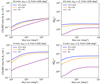 |
Fig. 10. Same as Fig. 7, but with a FoV of 100 deg2 using CTA-MST divergent pointing operation. The individual telescopes in the sub-array are pointed with an offset (i.e., 3°) to obtain a larger FoV. |
3.2.4. Mosaic strategy
The MST array is best suited for the mosaic strategy due to a FoV that is three times larger than the LST. The proposal for this scenario is the following: in order to cover a sky area of 100 deg2, we consider three pointings of MST which requires a total of 60 s. The slew between these three pointings requires ∼5 s, considering the slew time of MST to be 90 s to move to any point in the visible sky. Considering the same strategy of using pre-merger alerts and being on source at the merger time, the mosaic strategy maintains the same detection efficiency for short (< 20 s) VHE emission, but it requires a 30% more CTA time with respect to the one-shot observation. However, this strategy becomes more efficient with respect to the one-shot observation strategy for longer signals, such as the afterglow emission.
With respect to the divergent pointing the mosaic strategy has the advantage of not reducing the sensitivity. However, the divergent pointing has the significant advantage of the larger FoV; to cover the same area the mosaic strategy needs more observational time. Knowing the emission properties, in particular the expected flux decay, it would be possible to precisely compare the mosaic and divergent observational strategies (by assuming a larger exposure for detecting also signals longer than 20 s). The emission properties are largely uncertain to make precise estimates. It is worth noting that in the case of longer signals, the mosaic strategy can also benefit by the detection of the classical GRB prompt emission in the KeV-MeV by high-energy satellites able to localize the source (Ronchini et al. 2022).
4. Models producing early TeV emission
4.1. GRB prompt emission
The prompt emission dissipation models are very uncertain (see Piran 2004, Kumar & Zhang 2015, and Zhang 2018 for a review). This is partially because the dominant radiative processes responsible for the observed GRB spectra are not identified. Both time-resolved and time-integrated spectra in the 10 keV–10 MeV energy band are typically well accounted for by two power laws smoothly connected at their peak energy Eγ of νFν (Band et al. 1993). The photon index below Eγ has a typical value of −1 for long GRBs and −0.7 for short GRBs (see, e.g., Nava et al. 2012). The spectra with these photon indices physically are harder than simple fast-cooling synchrotron emission spectra, and they are much softer than thermal spectra (Preece et al. 1998; Ghisellini et al. 2000). One can generally divide the prompt emission models into those that invoke standard synchrotron-based models with dissipation occurring above the GRB jet photosphere and those models that invoke sub-photospheric dissipation. The most discussed model is the internal shocks model, which suggests an internal dissipation of a jet above the photosphere with a Lorentz factor gradient. This model is based on the assumption that the jet is dominated by kinetic energy. Alternatively, the GRB jet could be highly magnetized and the dissipation may occur via magnetic reconnection. Due to the huge uncertainty in these models and the absence of a clear preference for one over another, we are forced to rely on simplified models that can account for the basic spectral and temporal features.
The most standard model for prompt emission assumes that synchrotron radiation from nonthermal electrons makes the GRB emission. It has become clearer that in order to explain the GRB spectra by the synchrotron model, one is forced to assume a marginally or slow cooling regime of radiation (Bošnjak et al. 2009; Kumar & McMahon 2008; Beniamini & Piran 2013; Oganesyan et al. 2017; Ravasio et al. 2019). The most recent studies on the broadband prompt emission spectra have found a low-energy hardening of the GRB spectra at 2–20 keV, but even at higher energies. The low-energy breaks are found only for long GRBs, while it was shown that short GRBs are best described by a simple power law below the spectral peak, with an index of −0.7, which corresponds to a slow cooling synchrotron regime of radiation (Ravasio et al. 2019). This is not true for a recent GRB 211211A with a kilonova emission (i.e., associated with a compact binary merger), where the spectra show a clear presence of low-energy breaks (Gompertz et al. 2023). Nevertheless, in a slow or marginally fast cooling regime of radiation, in the electron synchrotron scenario, the parameter space for the production of the prompt emission is at odds with our naive expectation from the GRB dissipation site. It requires (1) that the magnetic field in the GRB emitting region is very weak ∼10 G, (2) that only a fraction of electrons are accelerated (total number typically required ∼1049 electrons), (3) an extremely high energy of the accelerated electrons (typical Lorentz factor of electrons of γm ∼ 105), (4) a very large size of the dissipation region of Rγ ∼ 1016 cm and extreme Lorentz factors of the jet of Γ > 400. Given the extreme energies of electrons, the SSC emission will be deeply in the Klein-Nishina regime, since the characteristic Lorentz factor of electrons that reach the Klein-Nishina threshold  , where we assumed z = 1 and Eγ = 500 keV, typical for short GRBs. Therefore, the peak energy of SSC will be approximately at ≈γmΓmec2 ∼ 30 γm, 5Γ2.7 TeV. The relative TeV to MeV flux can be roughly estimated by the Compton parameter
  , where
  is the optical depth and
  is the suppression factor due to the Klein-Nishina cross section (Ando et al. 2008). By assuming the above-mentioned parameters, we have an estimate of Y ∼ 0.5 (i.e., SSC VHE component with comparable luminosity as the keV – MeV prompt emission). This means that we expect to always observe TeV emission comparable with MeV prompt emission. The very presence of TeV/Γ photons in the jet initiates the pair production, which further suppresses the SSC component. Razzaque et al. (2004) derives analytically two characteristic energy thresholds for the internal attenuation of VHE photons within the prompt emission region. The first threshold is
  GeV. Photons above E1 will be suppressed by the pair production with Eγ (i.e., with most of the photons produced by GRB). The second threshold is
  GeV, which comes from the pair production of VHE photons with lowest energy photons (with Eγ0) in the GRB spectrum, where δt is the minimum variability timescale measured in the rest frame of the GRB host and Δ = ln(2(2Eγ0Eγ)1/2/meΓ)−1. Photons above E2 survive due to the decrease in the pair production cross section for extremely high-energy photons. Clearly, the suppression of the TeV component strongly depends on the bulk Lorentz factor of a GRB and the low-energy characteristics of GRB spectra (i.e., below 10 keV). Therefore, we would expect very different TeV signals (or no TeV emission at all) from a GRB to a GRB (Beniamini & Piran 2013).
There are other channels that produce VHE photons from the prompt emission. Shock and reconnection acceleration would result in efficient acceleration of protons in GRB jets. Shock accelerated electrons radiate at most hmec3/2π2e2 = 22 MeV photons (in the comoving frame of the jet) via the synchrotron radiation, while protons can produce photons up to 41 GeV. Therefore, TeV photons can be produced by the proton synchrotron mechanism (Aharonian 2000). In proton-dominated jets (i.e., when the ratio of the fraction of protons to electrons exceeds 100), the TeV component from the protons can be as luminous as the MeV prompt emission component (about 1052 erg s−1; Asano et al. 2009). The proton synchrotron component is very sensitive to Γ, the magnetic field, and the proton-to-electron ratio. Recently, it was suggested that the usual MeV component can be produced by the proton synchrotron radiation (Ghisellini et al. 2020) if the magnetic field is strong (B ∼ 106 G; see also Florou et al. 2023). The TeV photons are also expected from the products of the photo-meson interaction or the proton-synchrotron radiation by itself. There are two channels for the photo-meson process:
 (7)
(7)
The ratio of the first to the second channel is 2:1 at the resonant energy and is equal when out of resonance. To obtain pγ interaction, the photon in the comoving frame of the proton should reach the energy threshold of ∼300 MeV, which corresponds to protons with the Lorentz factor of  assuming the peak of the GRB spectrum as the main source of target photons. The typical energy of a neutral pion (in the comoving frame of the jet) is correspondingly
  (i.e.,
  ). A neutral pion decays into two photons of energy of
  TeV. The luminosity of the VHE component from the decay of neutral pions can be roughly estimated by the photo-meson cooling time. This returns a quantity
  , which is the fraction of protons making to photo-meson process (see, e.g., Kimura 2022) and χ(α, β) is a function that depends on GRB spectral indices α and β. Assuming typical values of α = −1 and β = −2.3, we obtain
  . In the formulae, for fpγ we used the relation between the size of the dissipation region Rγ and its bulk Lorentz factor Γ, Rγ ≈ 2cΓ2δt, which assumes that the GRB variability δt is driven by the radial or angular spread of the emission. The luminosity of the VHE component due to the neutron pions decay is approximately ∼0.5Lisofpγfpξp, where fp is the fraction of protons with energies suitable for the photo-meson interactions and ξp is the baryon loading fraction of the GRB jet (i.e., the ratio of the energy in the nonthermal protons to the emitted energy in the MeV prompt emission). If we take into account the nondetection of TeV neutrinos from GRBs (Lucarelli et al. 2023), then fpξp < 1 and the TeV component would have a luminosity of < 0.03Liso, 52 for the above-mentioned parameters. One needs to carefully take into account the internal suppression of the VHE component, as discussed above (see recent developments by Rudolph et al. 2023 for the internal shock model with hadrons).
Alternatively to the internal shocks model, another possible scenario is that of a magnetically dominated jet, where most of the energy of the jet is in the magnetic field and some dissipation process occurs to transfer the magnetic field energy to the accelerated particles (e.g., via magnetic reconnection; Drenkhahn 2002; Lyutikov & Blandford 2003; Zhang & Yan 2011). Recent first-principle simulations of magnetically dominated plasma turbulence show that electrons are impulsively accelerated to Lorentz factors γ ≈ σe by magnetic reconnection in large-scale current sheets, where σe = UB/(nemec2) is the plasma magnetization with respect to the electron rest mass and UB is the magnetic energy density. Since the accelerating electric field is nearly aligned with the local magnetic field, the distribution of the particle pitch angles θ is strongly anisotropic, and synchrotron emission is suppressed. Then inverse-Compton (IC) scattering may be the dominant cooling process, even in magnetically dominated plasma. It was already known that the typical spectral slope of the GRB prompt emission can be produced by synchrotron if the emitting electrons radiate most of their energy via IC in the Klein-Nishina regime. However, if the particle pitch angle distribution is isotropic (as is usually assumed), this would require the radiation energy density to be much higher than the magnetic energy density, which is not possible in the magnetically dominated jet. Instead, if the pitch angle θ is small, the condition for the IC cooling to be dominant become us ≫ θ2UB, where us is the energy density of synchrotron photons, which may be easily satisfied even in magnetically dominated plasma. The luminosity of the IC component is a fraction  of the synchrotron luminosity, where Epk is the peak energy of the synchrotron spectrum. The spectrum of the IC peaks at
  TeV, with two breaks at
  TeV and
  GeV. Photons with energy EIC > EIC, KN can annihilate before escaping, reducing the luminosity of the VHE component. The derivation of the emission of the secondary component from the created pairs requires a complex analysis, also considering the effect of the created pairs on the jet magnetization (Sobacchi et al. 2021). A detailed description of the production of the VHE emission from GRB can be found in Gill & Granot (2022) and references therein.
4.2. Afterglow emission
A few TeV sources during the afterglow emission have been detected by MAGIC and H.E.S.S. (Berti & Carosi 2022, and references therein). The afterglow TeV emission is interpreted as the SSC component from the electrons accelerated in the forward shock caused by the propagation of the GRB jet in the circumburst medium. This emission component depends on the microphysical parameters of the external shock and on the density of the circumburst medium. To date, TeV emission has been identified at relatively late times. The fastest slewing time so far is around 25 s for GRB 160821B (Acciari et al. 2021). Even though the SSC is the most obvious interpretation for the late TeV component, there are alternatives due to unclear observational distinction between synchrotron and SSC components. Surprisingly, the SSC component has a comparable amplitude to the synchrotron component. Apart from being a coincidence, due to microphysical parameters (low magnetic fields and small fraction of accelerated electrons), this can also be an indication of nontrivial acceleration processes (H. E. S. S. Collaboration 2021) or self-regulation of the external shock by the pairs (Derishev & Piran 2021). Therefore, it is extremely important to detect the TeV component from the forward shock from the early times. This will allow us to (1) constrain the total energetics of the jet, (2) constrain the initial bulk Lorentz factor, and (3) trace the evolution of the micro-physical parameters (Derishev & Piran 2021; for more details on the modeling of the VHE afterglow component from the forward shock accelerated electrons, see a recent review by Miceli & Nava 2022).
A less explored mechanism for the production of early VHE components is the reverse shock. The reverse shock forms at the earliest stages of the deceleration of the jet in the circumburst medium. Since the GRB jet is denser than the circumburst medium, the reverse shock is expected to accelerate electrons to lower energies. The synchrotron emission from the reverse shock is expected to produce a bright optical flash in the first tens of s from GRB detection (Mészáros & Rees 1997). Several bright optical flashes have been interpreted as arising from the reverse shock (see the list of GRBs with optical flashes in Oganesyan et al. 2023). However, some GRBs lack these optical flashes, even if well monitored at very early times. One interesting possibility is that the reverse shock develops in these jets, but the ongoing MeV prompt emission produced behind the reverse shock cools down the hot electrons, extracting their energy by the external inverse Compton (EIC) mechanism rather than the synchrotron emission (Beloborodov 2005). This is possible only if the reverse shock occurs in the relativistic regime (i.e., the duration of GRB is  s). We never witnessed an early optical flash from SGRBs simply due to instrumental difficulty to follow up a GRB of the second duration. However, given that a large fraction of SGRBs have soft extended emission, one can still have a source of prompt emission photons to cool down reverse shock accelerated electrons via EIC. There are other promising sources of EIC emission in the presence of long-lasting central engines (Murase et al. 2018; Zhang et al. 2021) or in the presence of the cocoon (Kimura et al. 2019).
4.3. Delayed pair echoes emission
Very-high-energy photons emitted either in the prompt or afterglow emission can annihilate with photons from extragalactic background light (EBL) with energy  eV over the mean free path length
  Mpc. The electron and positron produced share the energy of the VHE photon, and they can upscatter the photons from the cosmic microwave background (CMB) via IC up to energies
  GeV. Here we used that γe = EVHE(1 + z)/2mec2 ≈ 106(1 + z)E1 TeV and ECMB(z)≈6.35 × 10⁻⁴(1 + z) eV.
This secondary HE emission is called pair echoes (Aharonian et al. 1994; Plaga 1995; Takahashi et al. 2008; Murase et al. 2009), and it arrives with a characteristic time delay with respect to the primary VHE component due to the deflection of the pairs by the intergalactic magnetic field (IGMF). The pairs undergo IC cooling over a characteristic distance  Mpc. Assuming that the pair front expands spherically over a distance λIC with particles with Lorentz factors γe, the radial delay of the pair echoes with respect to the primary VHE emission is on the order of
  s for z = 1. Assuming maximum energy of the intrinsic GRB spectrum of
  TeV and z = 1, the maximum energy of the produced pair is ∼5 TeV and the up-scattered CMB photons can reach ≈100 GeV. The detection of the pair echoes would allow us to reconstruct the characteristics of the primary VHE component and probe the structure of the IGMF. Nonobservation of GeV photons from persistent sources such as TeV blazars allowed a lower limit of BIGMF > 10−16 G for a coherence length of 10 kpc (Neronov & Vovk 2010; Ackermann et al. 2018). However, for persistent sources, it is difficult to discriminate if the GeV photons observed are produced via pair echoes or via the intrinsic emission mechanism of the blazar, while the impulsive nature of the GRB can allow a clear temporal separation between these two components and serve as a better probe of the IGMF.
5. Conclusions
In this work we explored the possibility of detecting the earliest VHE emission associated with a binary system of neutron stars. To date, no prompt VHE emission has been detected from short GRBs, and the use of the GW signal from BNS can represent a unique way to search for it effectively. While the ability to detect such emission is largely limited for current GW and VHE observatories, our analysis shows that the future generation of GW detectors, such as ET and CE, operating in synergy with the next generation of VHE instruments, such as CTA, will provide the instrumental capabilities that make prompt VHE detections a reality. The search for the VHE counterpart will benefit from the GW pre-merger alerts made possible by accessing lower GW frequency observations, the much better sensitivity of next-generation GW and VHE observatories, and the large FoV, fast response, and slewing time of the VHE instruments.
We summarize the key points of our study as follows:
-
Pre-merger alerts and sky-localization capabilities of ET and network of GW detectors. A Fisher Matrix (GWFish; Dupletsa et al. 2023) approach was used to estimate the capabilities of the next generation of GW detectors to detect and localize binary-neutron star mergers. We explored the scenario to detect and localize BNSs pre-merger (during the inspiral phase) considering ET observing as a single detector, ET observing in a network with the current generation of detectors (LIGO, Virgo, KAGRA, and LIGO-India), ET with Voyager, and ET with one or two CEs. ET as a single observatory is able to detect several tens of BNSs per year with sky-localization smaller than 100 deg2 15 min before the merger; the number of detections increases to hundreds 5 and 1 min before the merger. While the presence of the current GW detectors (LVKI) or two Voyager operating with ET do not change the ET capability 15 and 5 min before the merger, at 1 min before the merger ET+LVKI (ET+2 VOY) increase by 17% (40%) the events localized better than 100 deg2 with respect to ET alone. The number of well-localized (< 100 deg2) events pre-merger is significantly higher when ET observes in a network of two or three third-generation detectors: hundreds of relatively well-localized detections 15 min before the merger, and several thousand detections 5 and 1 min before the merger. The absolute numbers are given in Table 2. In terms of redshifts, 5 min before the merger the well-localized (< 100 deg2) events reach a redshift of 0.4 for ET alone, 0.5 ET+CE, and 0.6 ET+2CE. The reached redshifts increase to 0.5 (ET alone), 1.0 (ET+CE), and 1.3 (ET+2CE) for events detected 1 min before the merger. ET alone is already able to detect a large number of well-localized pre-merger events, however, operating in a network of next-generation detectors will significantly increase this number and the redshifts up to which well-localized detections are possible.
-
CTA capability to detect the eraliest VHE emission from GRBs. The next generation IACT, CTA (consisting of three sub-arrays: LST, MST, SST) is expected to reach an order of magnitude better sensitivity than current VHE facilities. We evaluated the minimum energy requirement (
 ) of a short-lived burst for 10 s to be observed with CTA for a range of redshifts from 0.01 to 1.5 in the energy band of 0.2–1 TeV as the one observed by MST and LST. As described in Sect 2.4, we found that the minimum isotropic energy required for an event to be detected is ∼1043 erg, ∼1045 erg, ∼1047 erg, and ∼1051 erg at the redshift of 0.001, 0.01, 0.1, and 1.0, respectively. This energy range is consistent with the VHE emission scenarios described in Sect. 4.
 -
CTA observational strategies to detect the earliest VHE emission from BNS mergers. Taking into account the FoV and slewing time of MST and LST, we proposed three observational strategies to follow up on pre-merger alerts given by the GW detectors: (a) the direct pointing strategy following up all the events with sky-localization smaller than the FoV, that is 30 deg2 for MST and 10 deg2 for LST; (b) the one-shot observational strategy consisting of following up a large number of triggers using a single observation randomly located within the sky-localization uncertainty of the GW signals; and (c) the mosaic strategy tiling the sky-localization more effectively to detect the afterglow emission. Due to the longer slewing time of MST (tslew = 90 s), the 1 min of pre-merger alerts are followed up only with LST (tslew = 20 s). For the one-shot observational strategy, Tables 4 and 5 summarize the different paths to follow up pre-merger alert events with CTA-MST and CTA-LST, respectively. We considered following up (1) all the events detected 15 min before the merger, (2) all the events detected 5 min before the merger, (3) all the events detected 1 min before the merger (only LST), and (4) using the improved sky-localization updated 1 min before the merger for events detected 15 and 5 min pre-merger. Since the VHE emission is expected along the relativistic jet, we evaluated a strategy to prioritize alerts and increase the probability of detecting on-axis events. Taking into account the uncertainty on the viewing angle estimated pre-merger, we selected that all the events with an observed viewing angle smaller than 45° should be followed up.
-
Expected number of detection by MST and LST using the direct pointing strategy. Following up the events detected with sky-localization smaller than 10 deg2 1 min before the merger (a few hundred for ET+CE and several hundred for ET+2CE, see Table 2) using LST, we find that a few (ET+CE) to several (ET+CE) tens are expected to be on-axis (see Table 2), namely events with a viewing angle smaller than 10° from which we expect to observe the VHE emission. The number of on-axis events is negligible for ET alone, ET in a network with current generation detectors, or upgraded instruments such as Voyager. It is also negligible following up 15 and 5 min pre-merger alerts by ET in a network of two to three third-generation detectors. MST is able to observe a few tens of on-axis events following up a few hundred (several hundred) events detected 5 min before the merger with sky-localization smaller than 30 deg2. Taking into account the CTA duty cycle of 15% and the CTA visibility which reduces the observable sky by a factor 2, also assuming that all the BNS produce a jet, a few joint detections are expected using the direct pointing strategy only when ET is operating within a network of three third-generation detectors. We find that the direct pointing strategy is not so effective, also for ET in a network of third-generation detectors.
-
Expected number of detection by MST and LST using the one-shot observation strategy. The expected numbers of possible VHE detections by MST and LST per year and the corresponding CTA time required using the one-shot observation strategy are shown in Figs. 7 and 8, respectively. The plotted numbers take into account the CTA duty cycle of 15% and the CTA visibility. The CTA time includes slewing time, repositioning time, and exposure time. Using pre-merger 5 min alerts, we expect to detect around ten VHE possible counterparts per year by CTA-MST operating with ET+CE and ET+2CE by following events with sky-localization smaller than 103 deg2 at the cost of 25% (ET+CE) and 40% (ET+2CE) CTA time. Another 10 (20) possible VHE counterparts are expected using 1 min pre-merger alerts by following the events with LST with sky-localization smaller than about 200 deg2 detected by ET+CE (ET+2CE) at the expense of 20% (10%) of the CTA time. Only following pre-merger alerts of 1 min can give a few detections for ET as a single observatory or operating in the network ET+LVKI+ and LVK+2VOY. A significant reduction of the required CTA time can be obtained by prioritizing the alerts to be followed on the basis of the viewing angle estimate (expected to be given in the GW alert) and its uncertainty; following up the events with a viewing angle smaller then 45° reduces the required CTA time of about a factor 3. The effectiveness of this search increases by using updated information on the source parameters; that is using updated sky-localization available 1 min before the merger following up 15 or 5 min pre-merger alerts. Using MST, the expected number of possible VHE counterparts using updated information becomes 20 per year for ET+CE and 40 per year for ET+2CE following 5 min pre-merger alerts with sky-localization smaller than 103 deg2. For LST, following 5 min pre-merger alerts and updated information enable us to detect 10 (20) possible VHE counterparts are expected with CTA operating with ET+CE (ET+2CE). In addition, using the divergent pointing (single telescopes pointing slightly offset, and thus significantly enlarging the FoV) will be highly beneficial for observation, particularly in the case of large localizations 100–1000 deg2. With the expense of the same amount of MST-time of around 10% (< 1%) for a network of ET and CE (ET alone), divergent pointing is expected to follow up a factor of 6 (4) more on-axis events than MST (see Fig. 10) bringing the possible VHE detection to 60 (4) per year. However, the number of real detections will be influenced by the sensitivity, and the divergent pointing sensitivity is compromised with respect to the MST array as individual telescopes will be operated separately (the expected sensitivity reduction is of 20–25% for an offset of 3°).
-
Expected number of detections by MST and LST using mosaic observational strategy. The observational mosaic strategy, which tries to rapidly cover the entire sky-localization, can be more effective than the one-shot observation strategy for signals longer than 20 s, such as an afterglow emission. In the case of long signals, this strategy can significantly benefit from the presence of keV-MeV detection by high-energy satellites able to better localize the source.
-
Origin of VHE emission. Several emission scenarios envisage the possibility of producing the prompt VHE emission of GRBs. In the standard fireball model, while the MeV component is produced by electron synchrotron radiation in a marginally fast cooling regime, the same electrons are expected to emit a VHE component via SSC of intensity comparable to that of the MeV component. Another possibility is given in the scenario in which the prompt emission is produced by proton synchrotron, which can reach GeV energies in the jet comoving frame. The TeV component is the expected product of photo-meson interactions, emitting VHE photons via pion decay. In both these scenarios the VHE component is strongly dependent on the bulk Lorentz factor, magnetic field, electron-proton ratio, and lower-energy characteristics of the spectrum. Thus, different VHE emission is expected for different GRBs. Furthermore, pair production within the jet and, at higher redshift, with the extragalactic background light and cosmic microwave background is expected to attenuate its intensity. In the afterglow phase, the observed VHE photons can be interpreted as SSC from the forward shock, but a synchrotron origin associated with nontrivial acceleration processes is not excluded. The reverse shock may also be able to produce VHE emission via the EIC mechanism, offering an interpretation of the GRBs observed only in the VHE with no counterpart in the keV-MeV band (orphan GRBs). Furthermore, VHE photons coming either from prompt or afterglow emission can annihilate with lower energy photons, but the pair produced can up-scatter photons from the cosmic microwave background up to ∼100 GeV. This delayed component can be used to reconstruct the primary VHE emission and to probe the intergalactic magnetic field.
In summary, our work demonstrates that the next generation of GW observatories operating in synergy with VHE arrays, such as CTA, provides a unique opportunity to detect the prompt VHE counterpart of binary neutron star mergers. The results show that pre-merger alerts and rapid communication, response, and slewing time are essential. The presence of a network of third-generation detectors can significantly increase the effectiveness of this search by greatly increasing the number of possible detections per year with respect to a single third-generation detector operating alone or in a network of second-generation GW detectors. Prioritizing the events to be followed up on the basis of the source parameters estimated by the GW signals and giving updates on these parameters before the merger can greatly enhance the chance of detection, reducing the time request on EM observatories. Detecting the VHE prompt emission is crucial to understanding the physics governing the GRB engine.
The code is publicly available at this repository https://github.com/janosch314/GWFish
The sum is done over events with sky-localization smaller than a threshold (Ω) in order to obtain the cumulative number of VHE counterparts as a function of this threshold. This threshold can be used in real observations to decide what GW triggers to be followed.
Acknowledgments
We acknowledge Stefano Bagnasco, Federica Legger, Sara Vallero, and the INFN Computing Center of Turin for providing support and computational resources. We thank Yann Bouffanais for the work and help on the population of BNSs. B.B. and M.B. acknowledge financial support from the Italian Ministry of University and Research (MUR) for the PRIN grant METE under contract no. 2020KB33TP. B.B. acknowledges financial support from the Italian Ministry of University and Research (MUR) (PRIN 2017 grant 20179ZF5KS). M.B. and G.O. acknowledge financial support from the AHEAD2020 project (grant agreement n. 871158). M.M. and F.S. acknowledge financial support from the European Research Council for the ERC Consolidator grant DEMOBLACK, under contract no. 770017.
References
- Abbott, B. P., Abbott, R., Abbott, T. D., et al. 2017a, ApJ, 848, L13 [CrossRef] [Google Scholar]
- Abbott, B. P., et al. (LIGO Scientific Collaboration& Virgo Collaboration) 2017b, Phys. Rev. Lett., 119, 161101 [CrossRef] [Google Scholar]
- Abbott, B. P., Abbott, R., Abbott, T. D., et al. 2017c, ApJ, 848, L12 [Google Scholar]
- Abbott, B. P., Abbott, R., Abbott, T. D., et al. 2017d, Class. Quant. Grav., 34, 044001 [NASA ADS] [CrossRef] [Google Scholar]
- Abbott, B. P., Abbott, R., Abbott, T. D., et al. 2019, ApJ, 875, 161 [NASA ADS] [CrossRef] [Google Scholar]
- Abbott, B. P., Abbott, R., Abbott, T. D., et al. 2020, Liv. Rev. Relati., 23, 3 [Google Scholar]
- Abbott, B. P., et al. (LIGO Scientific Collaboration, Virgo Collaboration,& KAGRA Collaboration) 2023, Phys. Rev. X, 13, 011048 [NASA ADS] [Google Scholar]
- Abdalla, H., Abramowski, A., Aharonian, F., et al. 2017, ApJ, 850, L22 [NASA ADS] [CrossRef] [Google Scholar]
- Abdalla, H., Adam, R., Aharonian, F., et al. 2019, Nature, 575, 464 [Google Scholar]
- Abdalla, H., Adam, R., Aharonian, F., et al. 2020, ApJ, 894, L16 [NASA ADS] [CrossRef] [Google Scholar]
- Acciari, V. A., Ansoldi, S., Antonelli, L. A., et al. 2021, ApJ, 908, 90 [NASA ADS] [CrossRef] [Google Scholar]
- Ackermann, M., Ajello, M., Baldini, L., et al. 2018, ApJS, 237, 32 [NASA ADS] [CrossRef] [Google Scholar]
- Actis, M., Agnetta, G., Aharonian, F., et al. 2011, Exp. Astron., 32, 193 [NASA ADS] [CrossRef] [Google Scholar]
- Adhikari, R. X., Arai, K., Brooks, A. F., et al. 2020, Classical Quantum Gravity, 37, 165003 [NASA ADS] [CrossRef] [Google Scholar]
- Aharonian, F. A. 2000, New A, 5, 377 [NASA ADS] [CrossRef] [Google Scholar]
- Aharonian, F. A., Coppi, P. S., & Voelk, H. J. 1994, ApJ, 423, L5 [NASA ADS] [CrossRef] [Google Scholar]
- Aleksić, J., Ansoldi, S., Antonelli, L. A., et al. 2016a, Astropart. Phys., 72, 76 [Google Scholar]
- Aleksić, J., Ansoldi, S., Antonelli, L. A., et al. 2016b, Astropart. Phys., 72, 61 [Google Scholar]
- Alexander, K. D., Margutti, R., Blanchard, P. K., et al. 2018, ApJ, 863, L18 [NASA ADS] [CrossRef] [Google Scholar]
- Ando, S., Nakar, E., & Sari, R. 2008, ApJ, 689, 1150 [NASA ADS] [CrossRef] [Google Scholar]
- Asano, K., & Inoue, S. 2007, ApJ, 671, 645 [NASA ADS] [CrossRef] [Google Scholar]
- Asano, K., Inoue, S., & Meszaros, P. 2009, ApJ, 699, 953 [CrossRef] [Google Scholar]
- Band, D., Matteson, J., Ford, L., et al. 1993, ApJ, 413, 281 [Google Scholar]
- Bartos, I., Corley, K. R., Gupte, N., et al. 2019, MNRAS, 490, 3476 [Google Scholar]
- Beloborodov, A. M. 2005, ApJ, 627, 346 [NASA ADS] [CrossRef] [Google Scholar]
- Beloborodov, A. M. 2013, ApJ, 764, 157 [NASA ADS] [CrossRef] [Google Scholar]
- Beniamini, P., & Piran, T. 2013, ApJ, 769, 69 [Google Scholar]
- Bernlöhr, K., Barnacka, A., Becherini, Y., et al. 2013, Astropart. Phys., 43, 171 [Google Scholar]
- Berti, A., & Carosi, A. 2022, Galaxies, 10, 67 [CrossRef] [Google Scholar]
- Bošnjak, Ž., Daigne, F., & Dubus, G. 2009, A&A, 498, 677 [NASA ADS] [CrossRef] [EDP Sciences] [Google Scholar]
- Branchesi, M., Maggiore, M., Alonso, D., et al. 2023, JCAP, 07, 068 [CrossRef] [Google Scholar]
- Buonanno, A., Iyer, B. R., Ochsner, E., Pan, Y., & Sathyaprakash, B. S. 2009, Phys. Rev. D, 80, 084043 [NASA ADS] [CrossRef] [Google Scholar]
- Burgay, M., D’Amico, N., Possenti, A., et al. 2003, Nature, 426, 531 [NASA ADS] [CrossRef] [Google Scholar]
- Cannon, K., Cariou, R., Chapman, A., et al. 2012, ApJ, 748, 136 [CrossRef] [Google Scholar]
- Cao, Z., della Volpe, D., & Liu, S., et al. 2019, Chin. Phys. C, 46, 035001 [Google Scholar]
- Chan, M. L., Messenger, C., Heng, I. S., & Hendry, M. 2018, Phys. Rev. D, 97, 123014 [NASA ADS] [CrossRef] [Google Scholar]
- Chatziioannou, K., Cornish, N., Wijngaarden, M., & Littenberg, T. B. 2021, Phys. Rev. D, 103, 044013 [NASA ADS] [CrossRef] [Google Scholar]
- Cherenkov Telescope Array Consortium (Acharya, B. S., et al.) 2019, Science with the Cherenkov Telescope Array [Google Scholar]
- Chu, Q., Kovalam, M., Wen, L., et al. 2022, Phys. Rev. D, 105, 024023 [NASA ADS] [CrossRef] [Google Scholar]
- Colombo, A., Salafia, O. S., Gabrielli, F., et al. 2022, ApJ, 937, 79 [NASA ADS] [CrossRef] [Google Scholar]
- Derishev, E., & Piran, T. 2021, ApJ, 923, 135 [CrossRef] [Google Scholar]
- Derishev, E. V., Kocharovsky, V. V., & Kocharovsky, V. V. 2001, A&A, 372, 1071 [NASA ADS] [CrossRef] [EDP Sciences] [Google Scholar]
- Domínguez, A., Primack, J. R., Rosario, D. J., et al. 2011, MNRAS, 410, 2556 [Google Scholar]
- Donini, A., Gasparetto, T., Bregeon, J., et al. 2019, Int. Cosmic Ray Conf., 36, 664 [NASA ADS] [CrossRef] [Google Scholar]
- Drenkhahn, G. 2002, A&A, 387, 714 [NASA ADS] [CrossRef] [EDP Sciences] [Google Scholar]
- Dupletsa, U., Harms, J., Banerjee, B., et al. 2023, Astron. Comput., 42, 100671 [NASA ADS] [CrossRef] [Google Scholar]
- Eichler, D., & Levinson, A. 2000, ApJ, 529, 146 [NASA ADS] [CrossRef] [Google Scholar]
- Evans, M., Adhikari, R. X., Afle, C., et al. 2021, ArXiv e-prints [arXiv:2109.09882] [Google Scholar]
- Florou, I., Petropoulou, M., & Mastichiadis, A. 2021, MNRAS, 505, 1367 [Google Scholar]
- Florou, I., Mastichiadis, A., & Petropoulou, M. 2023, MNRAS, 521, 5583 [Google Scholar]
- Fryer, C. L., Belczynski, K., Wiktorowicz, G., et al. 2012, ApJ, 749, 91 [Google Scholar]
- Galvan-Gamez, A., Fraija, N., & Gonzalez, M. M. 2020, PoS, ICRC2019, 681 [Google Scholar]
- Gérard, L. 2015, Int. Cosmic Ray Conf., 34, 725 [Google Scholar]
- Ghirlanda, G., Celotti, A., & Ghisellini, G. 2003, A&A, 406, 879 [NASA ADS] [CrossRef] [EDP Sciences] [Google Scholar]
- Ghirlanda, G., Salafia, O. S., Paragi, Z., et al. 2019, Science, 363, 968 [NASA ADS] [CrossRef] [Google Scholar]
- Ghisellini, G., Celotti, A., & Lazzati, D. 2000, MNRAS, 313, L1 [NASA ADS] [CrossRef] [Google Scholar]
- Ghisellini, G., Ghirlanda, G., Oganesyan, G., et al. 2020, A&A, 636, A82 [NASA ADS] [CrossRef] [EDP Sciences] [Google Scholar]
- Giacobbo, N., & Mapelli, M. 2018, MNRAS, 480, 2011 [Google Scholar]
- Giacobbo, N., & Mapelli, M. 2019, MNRAS, 482, 2234 [Google Scholar]
- Giacobbo, N., & Mapelli, M. 2020, ApJ, 891, 141 [NASA ADS] [CrossRef] [Google Scholar]
- Giacobbo, N., Mapelli, M., & Spera, M. 2018, MNRAS, 474, 2959 [Google Scholar]
- Giannios, D. 2012, MNRAS, 422, 3092 [Google Scholar]
- Gill, R., & Granot, J. 2022, Galaxies, 10, 74 [CrossRef] [Google Scholar]
- Goldstein, A., Veres, P., Burns, E., et al. 2017, ApJ, 848, L14 [CrossRef] [Google Scholar]
- Gompertz, B. P., Ravasio, M. E., Nicholl, M., et al. 2023, Nat. Astron., 7, 67 [Google Scholar]
- Goncharov, B., Nitz, A. H., & Harms, J. 2022, Phys. Rev. D, 105, 122007 [NASA ADS] [CrossRef] [Google Scholar]
- Goodman, J. 1986, ApJ, 308, L47 [NASA ADS] [CrossRef] [Google Scholar]
- Guetta, D., & Granot, J. 2003, ApJ, 585, 885 [CrossRef] [Google Scholar]
- Gupta, N., & Zhang, B. 2007, MNRAS, 380, 78 [Google Scholar]
- H. E. S. S. Collaboration (Abdalla, H., et al.) 2021, Science, 372, 1081 [NASA ADS] [CrossRef] [Google Scholar]
- Hallinan, G., Corsi, A., Mooley, K. P., et al. 2017, Science, 358, 1579 [NASA ADS] [CrossRef] [Google Scholar]
- Hild, S., Abernathy, M., Acernese, F., et al. 2011, Classical Quantum Gravity, 28, 094013 [NASA ADS] [CrossRef] [Google Scholar]
- Hobbs, G., Lorimer, D. R., Lyne, A. G., & Kramer, M. 2005, MNRAS, 360, 974 [Google Scholar]
- Iacovelli, F., Mancarella, M., Foffa, S., & Maggiore, M. 2022, ApJ, 941, 208 [NASA ADS] [CrossRef] [Google Scholar]
- Kimura, S. S. 2022, ArXiv e-prints [arXiv:2202.06480] [Google Scholar]
- Kimura, S. S., Murase, K., Ioka, K., et al. 2019, ApJ, 887, L16 [NASA ADS] [CrossRef] [Google Scholar]
- Kouveliotou, C., Meegan, C. A., Fishman, G. J., et al. 1993, ApJ, 413, L101 [NASA ADS] [CrossRef] [Google Scholar]
- Kumar, P., & McMahon, E. 2008, MNRAS, 384, 33 [NASA ADS] [CrossRef] [Google Scholar]
- Kumar, P., & Zhang, B. 2015, Phys. Rep., 561, 1 [Google Scholar]
- La Mura, G., Chiaro, G., Conceição, R., et al. 2020, MNRAS, 497, 3142 [Google Scholar]
- Lennarz, D., & Taboada, I. 2015, Int. Cosmic Ray Conf., 34, 715 [NASA ADS] [Google Scholar]
- Levinson, A., & Eichler, D. 1993, ApJ, 418, 386 [NASA ADS] [CrossRef] [Google Scholar]
- Li, T. P., & Ma, Y. Q. 1983, ApJ, 272, 317 [CrossRef] [Google Scholar]
- Li, Y., Heng, I. S., Chan, M. L., Messenger, C., & Fan, X. 2022, Phys. Rev. D, 105, 043010 [NASA ADS] [CrossRef] [Google Scholar]
- LIGO Scientific Collaboration (Aasi, J., et al.) 2015, Classical Quantum Gravity, 32, 074001 [NASA ADS] [CrossRef] [Google Scholar]
- Lloyd, N. M., & Petrosian, V. 2000, ApJ, 543, 722 [NASA ADS] [CrossRef] [Google Scholar]
- López-Coto, R., Moralejo, A., Artero, M., et al. 2021, ArXiv e-prints [arXiv:2109.03515] [Google Scholar]
- Lucarelli, F., Oganesyan, G., Montaruli, T., et al. 2023, A&A, 672, A102 [NASA ADS] [CrossRef] [EDP Sciences] [Google Scholar]
- Lyman, J. D., Lamb, G. P., Levan, A. J., et al. 2018, Nat. Astron., 2, 751 [NASA ADS] [CrossRef] [Google Scholar]
- Lyutikov, M., & Blandford, R. 2003, ArXiv e-prints [arXiv:astro-ph/0312347] [Google Scholar]
- Madau, P., & Fragos, T. 2017, ApJ, 840, 39 [Google Scholar]
- Magee, R., Chatterjee, D., Singer, L. P., et al. 2021, ApJ, 910, L21 [NASA ADS] [CrossRef] [Google Scholar]
- Maggiore, M., Van Den Broeck, C., Bartolo, N., et al. 2020, JCAP, 03, 050 [CrossRef] [Google Scholar]
- MAGIC Collaboration (Acciari, V. A., et al.) 2019, Nature, 575, 455 [Google Scholar]
- Mapelli, M., Giacobbo, N., Ripamonti, E., & Spera, M. 2017, MNRAS, 472, 2422 [NASA ADS] [CrossRef] [Google Scholar]
- Meszaros, P., & Rees, M. J. 1992, MNRAS, 257, 29P [NASA ADS] [CrossRef] [Google Scholar]
- Mészáros, P., & Rees, M. J. 1997, ApJ, 476, 232 [CrossRef] [Google Scholar]
- Miceli, D., & Nava, L. 2022, Galaxies, 10, 66 [NASA ADS] [CrossRef] [Google Scholar]
- Miceli, D., Antonelli, L. A., Becerra Gonzalez, J., et al. 2019, Int. Cosmic Ray Conf., 36, 743 [NASA ADS] [CrossRef] [Google Scholar]
- Montaruli, T., Pareschi, G., & Greenshaw, T. 2015, ArXiv e-prints [arXiv:1508.06472] [Google Scholar]
- Mooley, K. P., Deller, A. T., Gottlieb, O., et al. 2018, Nature, 561, 355 [Google Scholar]
- Murase, K., Zhang, B., Takahashi, K., & Nagataki, S. 2009, MNRAS, 396, 1825 [Google Scholar]
- Murase, K., Toomey, M. W., Fang, K., et al. 2018, ApJ, 854, 60 [NASA ADS] [CrossRef] [Google Scholar]
- Nakar, E., Ando, S., & Sari, R. 2009, ApJ, 703, 675 [NASA ADS] [CrossRef] [Google Scholar]
- Narayan, R., Paczynski, B., & Piran, T. 1992, ApJ, 395, L83 [NASA ADS] [CrossRef] [Google Scholar]
- Nava, L., Salvaterra, R., Ghirlanda, G., et al. 2012, MNRAS, 421, 1256 [Google Scholar]
- Neronov, A., & Vovk, I. 2010, Science, 328, 73 [NASA ADS] [CrossRef] [Google Scholar]
- Nitz, A. H., & Dal Canton, T. 2021, ApJ, 917, L27 [NASA ADS] [CrossRef] [Google Scholar]
- Oganesyan, G., Nava, L., Ghirlanda, G., & Celotti, A. 2017, ApJ, 846, 137 [Google Scholar]
- Oganesyan, G., Karpov, S., Salafia, O. S., et al. 2023, Nat. Astron., 7, 2397 [Google Scholar]
- Paczynski, B. 1986, ApJ, 308, L43 [NASA ADS] [CrossRef] [Google Scholar]
- Paczynski, B., & Rhoads, J. E. 1993, ApJ, 418, L5 [NASA ADS] [CrossRef] [Google Scholar]
- Papathanassiou, H., & Meszaros, P. 1996, ApJ, 471, L91 [NASA ADS] [CrossRef] [Google Scholar]
- Patricelli, B., Stamerra, A., Razzano, M., Pian, E., & Cella, G. 2018, J. Cosmology Astropart. Phys., 2018, 056 [CrossRef] [Google Scholar]
- Patricelli, B., Carosi, A., Nava, L., et al. 2022a, in 37th International Cosmic Ray Conference, 12-23 July 2021, Berlin, Germany, online at https://pos.sissa.it/cgi-bin/reader/conf.cgi?confid=395, 998 [Google Scholar]
- Patricelli, B., Bernardini, M. G., Mapelli, M., et al. 2022b, MNRAS, 513, 4159 [NASA ADS] [CrossRef] [Google Scholar]
- Pe’er, A., & Waxman, E. 2004, ApJ, 613, 448 [CrossRef] [Google Scholar]
- Pe’er, A., Mészáros, P., & Rees, M. J. 2006, ApJ, 642, 995 [CrossRef] [Google Scholar]
- Perna, R., Artale, M. C., Wang, Y.-H., et al. 2022, MNRAS, 512, 2654 [NASA ADS] [CrossRef] [Google Scholar]
- Pilla, R. P., & Loeb, A. 1998, ApJ, 494, L167 [CrossRef] [Google Scholar]
- Piran, T. 2004, Rev. Modern Phys., 76, 1143 [Google Scholar]
- Plaga, R. 1995, Nature, 374, 430 [NASA ADS] [CrossRef] [Google Scholar]
- Preece, R. D., Briggs, M. S., Mallozzi, R. S., et al. 1998, ApJ, 506, L23 [Google Scholar]
- Pühlhofer, G. 2017, AIP Conf. Ser., 1792 [Google Scholar]
- Punturo, M. M., Abernathy, F., Acernese, et al. 2010, Classical Quantum Gravity, 27, 194002 [CrossRef] [Google Scholar]
- Ravasio, M. E., Ghirlanda, G., Nava, L., & Ghisellini, G. 2019, A&A, 625, A60 [NASA ADS] [CrossRef] [EDP Sciences] [Google Scholar]
- Razzaque, S., Mészáros, P., & Zhang, B. 2004, ApJ, 613, 1072 [NASA ADS] [CrossRef] [Google Scholar]
- Rees, M. J., & Meszaros, P. 1992, MNRAS, 258, 41 [Google Scholar]
- Rees, M. J., & Meszaros, P. 1994, ApJ, 430, L93 [Google Scholar]
- Reitze, D., Adhikari, R. X., Ballmer, S., et al. 2019, Bull. Am. Astron. Soc., 51, 035 [Google Scholar]
- Ronchini, S., Branchesi, M., Oganesyan, G., et al. 2022, A&A, 665, A97 [NASA ADS] [CrossRef] [EDP Sciences] [Google Scholar]
- Rudolph, A., Petropoulou, M., Bošnjak, Ž., & Winter, W. 2023, ApJ, 950, 28 [NASA ADS] [CrossRef] [Google Scholar]
- Ryde, F. 2005, ApJ, 625, L95 [NASA ADS] [CrossRef] [Google Scholar]
- Sachdev, S., Magee, R., Hanna, C., et al. 2020, ApJ, 905, L25 [NASA ADS] [CrossRef] [Google Scholar]
- Salafia, O. S., Berti, A., Covino, S., et al. 2021, PoS, ICRC2021, 944 [Google Scholar]
- Salafia, O. S., Colombo, A., Gabrielli, F., & Mandel, I. 2022, A&A, 666, A174 [NASA ADS] [CrossRef] [EDP Sciences] [Google Scholar]
- Samajdar, A., Janquart, J., Van Den Broeck, C., & Dietrich, T. 2021, Phys. Rev. D, 104, 044003 [NASA ADS] [CrossRef] [Google Scholar]
- Santoliquido, F., Mapelli, M., Bouffanais, Y., et al. 2020, ApJ, 898, 152 [Google Scholar]
- Santoliquido, F., Mapelli, M., Giacobbo, N., Bouffanais, Y., & Artale, M. C. 2021, MNRAS, 502, 4877 [NASA ADS] [CrossRef] [Google Scholar]
- Sari, R., & Piran, T. 1997, MNRAS, 287, 110 [Google Scholar]
- Sari, R., Narayan, R., & Piran, T. 1996, ApJ, 473, 204 [Google Scholar]
- Sari, R., Piran, T., & Narayan, R. 1998, ApJ, 497, L17 [Google Scholar]
- Savchenko, V., Ferrigno, C., Kuulkers, E., et al. 2017, ApJ, 848, L15 [NASA ADS] [CrossRef] [Google Scholar]
- Seglar-Arroyo, M., Ashkar, H., Bonnefoy, S., et al. 2019a, Int. Cosmic Ray Conf., 36, 789 [NASA ADS] [CrossRef] [Google Scholar]
- Seglar-Arroyo, M., Bissaldi, E., Bulgarelli, A., et al. 2019b, Int. Cosmic Ray Conf., 36, 790 [NASA ADS] [CrossRef] [Google Scholar]
- Shemi, A., & Piran, T. 1990, ApJ, 365, L55 [NASA ADS] [CrossRef] [Google Scholar]
- Sobacchi, E., Sironi, L., & Beloborodov, A. M. 2021, MNRAS, 506, 38 [NASA ADS] [CrossRef] [Google Scholar]
- Stamerra, A., Patricelli, B., Bartos, I., & Branchesi, M. 2021, Multi-messenger Astrophysics with the Highest Energy Counterparts of Gravitational Waves, 5 [Google Scholar]
- Takahashi, K., Murase, K., Ichiki, K., Inoue, S., & Nagataki, S. 2008, ApJ, 687, L5 [NASA ADS] [CrossRef] [Google Scholar]
- Tavani, M. 1996, ApJ, 466, 768 [NASA ADS] [CrossRef] [Google Scholar]
- Thompson, C. 1994, MNRAS, 270, 480 [NASA ADS] [CrossRef] [Google Scholar]
- Troja, E., Piro, L., van Eerten, H., et al. 2017, Nature, 551, 71 [NASA ADS] [CrossRef] [Google Scholar]
- Usov, V. V. 1992, Nature, 357, 472 [NASA ADS] [CrossRef] [Google Scholar]
- Virgo Collaboration (Acernese, F., et al.) 2015, Classical Quantum Gravity, 32, 024001 [NASA ADS] [CrossRef] [Google Scholar]
- Yong, H., Shicong, H., Songzhan, C., et al. 2022, GRB Coordinates Network, 32677, 1 [Google Scholar]
- Zhang, B. 2018, The Physics of Gamma-Ray Bursts, (Cambridge University Press) [Google Scholar]
- Zhang, B. 2019, Front. Phys., 14, 64402 [NASA ADS] [CrossRef] [Google Scholar]
- Zhang, B., & Yan, H. 2011, ApJ, 726, 90 [Google Scholar]
- Zhang, B. T., Murase, K., Yuan, C., Kimura, S. S., & Mészáros, P. 2021, ApJ, 908, L36 [NASA ADS] [CrossRef] [Google Scholar]
Appendix A: Pessimistic and optimistic BNS population scenarios
Our results throughout the paper are given for a fiducial scenario that adopts a common envelope ejection efficiency parameter, αCE, equal to 3 (see section 2.1). Here we show the detection capabilities of ET as a single observatory and in network with other facilities such as LVKI+, CE, and 2CE using two populations, the pessimistic and optimistic BNS merger populations, obtained with a common envelope ejection efficiency parameter of α = 0.5 and α = 5. Figure A.1 shows the number of detections per year at different times before the merger, namely 15, 5, and 1 min, and at the merger time for ET as a single observatory and in the network of detectors. Figure A.2 shows the number of detections of on-axis BNS systems per year.
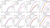 |
Fig. A.1. Cumulative number of detections (S/N> 8) per year for different networks of GW detectors considering 15, 5, and 1 min before the merger, and at the merger time considering the pessimistic (top row) and optimistic (bottom row) BNS merger population scenarios. The number of injected BNSs is set to 2.0 × 10⁴ and 4.0 × 10⁵ within redshift z = 1.5 for the pessimistic and optimistic scenarios, respectively. The plots show the detections considering BNS systems with all orientations. |
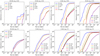 |
Fig. A.2. Same as Fig. A.1, but for the detections of BNS systems with a viewing angle smaller than 10° (on-axis events), a fraction of which are expected to produce detectable VHE emissions. |
Appendix B: GW alert prioritization based on the viewing angle
The next generation of GW observatories will detect a large number of events. To optimize the required observational time required by the EM observatories to follow them, it will be necessary to prioritize the events to be followed. In the case of VHE prompt emission expected from on-axis events a parameter that can be used is the viewing angle. In this Appendix we evaluate the precision of determining the viewing angle from GW observations. Figure B.1 shows the uncertainty on the viewing angle θv (Δθv) estimated by GWFish versus the injected viewing angle (θv) for different configurations of the network of GW detectors and at different times before the merger. As can be seen from the figure, the uncertainties are larger for on-axis events.
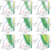 |
Fig. B.1. Distribution of uncertainties on viewing angle (Δθv) as estimated by GWFish vs injected θv of our fiducial population of BNS mergers for different detector configurations (ET, ET+CE, and ET+2CE) and for different pre-merger alert times (15 min, 5 min, 1 min) and at the time of the merger. The solid lines correspond to Δθv/θv = 0.1 and 0.5. The vertical color bar indicates the redshift of each event. The plots show only the BNS mergers below redshift 1.5. The uncertainty on the viewing angle, Δθv, is larger in the case of on-axis events. |
Appendix C: Improvement in sky-localization of the pre-merger events approaching merger time
For an event detected pre-merger, the estimate of the sky-localization improves as the event gets closer to merger time. Figure C.1 shows the systematic improvement of the sky-localization 1 min before the merger with respect to the sky-localizations obtained 15 min and 5 min before for the same events.
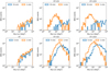 |
Fig. C.1. Improvement in sky-localization estimates closer to merger time. The blue histograms in the top panels show the sky-localizations obtained 15 min before the merger and in the bottom panels 5 min before the merger. The 1 min (orange) histograms show the sky-localization estimates for the same events. Re-positioning CTA within the updated (smaller) sky-localization released 1 min before the merger increases the chance of VHE detection. |
All Tables
Detector specification of CTA (α-configuration) as compared to the current-generation IACT (i.e., MAGIC).
Number of detected (network S/N > 8) BNS mergers per year within z = 1.5 for different GW detector configurations.
All Figures
|
Fig. 1. Evolution of the merger rate density in the comoving frame as a function of redshift for the BNS populations used in the present work. Our fiducial population is obtained with a common envelope efficiency αCE = 3 and is represented by the orange solid line. The pessimistic and optimistic populations are obtained with αCE = 0.5 and 5 and are shown by blue and green solid lines, respectively. The grey area shows the 90% credible interval of the local merger rate density, as inferred from the first three observing runs of LIGO, Virgo, and KAGRA (Abbott et al. 2023). |
| In the text | |
|
Fig. 2. General observation scheme for detection of the VHE prompt emission phase of the BNS merger. The low-frequency observations made possible by the next generation of GW detectors will enable an inspiraling BNS system to be detected and localized before the merger. A pre-merger alert for the event is sent and the VHE detectors can rapidly point to the target during the merger. The delay between the GW and VHE emission is assumed to be within our exposure time of 20 s. |
| In the text | |
|
Fig. 3. Intrinsic (assumed) and observed spectra for VHE transient events with specific spectral indices (Γ) and cutoff (Ec) for the isotropic energy |
| In the text | |
|
Fig. 4. Lower limit on isotropic energy (EISO) in the range 0.2–1 TeV as a function of redshift for CTA-N (α-configuration including four LSTs and nine MSTs). A short constant VHE emission of 10 s is considered, and a threshold is used on the significance (σ) of 5σ and on excess gamma-ray events (Nex) larger than 10 to define a detection. A conservative energy threshold of E > 200 GeV (hence a slightly higher limit on |
| In the text | |
|
Fig. 5. Cumulative number of detections (S/N > 8) per year for different networks of GW detectors considering 15, 5, and 1 min before the merger and at the merger time. The top panels show the detections considering BNS systems with all orientations. The bottom panels show the detections of BNS systems with a viewing angle smaller than 10° (on-axis events), a fraction of which are expected to produce detectable VHE emissions. For each of the simulations, the injected BNSs are within redshift z = 1.5. The quoted detection numbers refer to the fiducial population and are obtained assuming a duty cycle of 0.85 (see text). For the 15 and 5 min pre-merger scenarios, the ET+LVKI+ and ET+2VOY do not show any significant difference with respect to ET as a single observatory (the red and green lines lie under the purple line). |
| In the text | |
|
Fig. 6. Redshift distribution of sky-localization uncertainty (given as 90% credible region) for three detector configurations: ET, ET+CE, and ET+2CE. The absolute numbers refer to the fiducial BNS population sample and detections within a redshift of 1.5 per year of observation assuming a duty cycle of 0.85 (see text). The panels show the detections and the corresponding sky-localizations as a function of the redshift 15, 5, and 1 min before the merger and at the merger time. The blue histogram (“All”) shows all the detected sources. |
| In the text | |
|
Fig. 7. Expected number of detections by CTA-MST using the one-shot observation strategy (left column). The estimates of the number of possible VHE counterparts are based on the on-axis BNS systems (systems injected with θv < 10° in our simulations) and are evaluated as described in the text (see Eq. (6)). These estimates assume that all BNS produce a jet. They take into account the sky-localization (Ωi) of each event, the MST field of view of 30 deg2, the CTA duty cycle of 15%, and the CTA visibility limited to a zenith angle larger than 60° (minimum elevation of 30°). The fraction of CTA time spent following all the GW alerts with the sky-localization smaller than the one indicated on the x-axis is given by the plots in the central column. To observe each event (independent of the sky-localization) the observational time (tobs) is considered, given by the sum of slewing time (tslew = 90 s), an additional re-positioning time (trep = 10 s), and the exposure time (texp = 20 s). The plots in the right column show the CTA time when only triggers with an observed θv < 45° are followed up resulting in a significant reduction of CTA time. |
| In the text | |
|
Fig. 8. Same as Fig. 7, but considering LSTs. A FoV of ∼10 deg2 is used and the observational time for each event (tobs) of 50 s is given by the slewing time (tslew) of 20 s, an additional repositioning time of 10 s, and the exposure time (texp) of 20 s. Thanks to the rapid slew time for LST, we also consider the scenario where the 1 min pre-merger alerts are directly followed. |
| In the text | |
|
Fig. 9. Same as Figs. 7 and 8 following up 15 and 5 min pre-merger alerts, but using the updated sky-localization obtained 1 min before the merger. For this scenario, only events detected 15 min or 5 min before the merger with sky-localization less than 1000 deg2 are considered. The expected number of VHE possible detections includes the CTA visibility because LST and MST antennas are not able to observe below the elevation angle of 30° (zenith higher than 60°). The plots in the right column show the LST array and the plots in the left column the MST array. |
| In the text | |
|
Fig. 10. Same as Fig. 7, but with a FoV of 100 deg2 using CTA-MST divergent pointing operation. The individual telescopes in the sub-array are pointed with an offset (i.e., 3°) to obtain a larger FoV. |
| In the text | |
|
Fig. A.1. Cumulative number of detections (S/N> 8) per year for different networks of GW detectors considering 15, 5, and 1 min before the merger, and at the merger time considering the pessimistic (top row) and optimistic (bottom row) BNS merger population scenarios. The number of injected BNSs is set to 2.0 × 10⁴ and 4.0 × 10⁵ within redshift z = 1.5 for the pessimistic and optimistic scenarios, respectively. The plots show the detections considering BNS systems with all orientations. |
| In the text | |
|
Fig. A.2. Same as Fig. A.1, but for the detections of BNS systems with a viewing angle smaller than 10° (on-axis events), a fraction of which are expected to produce detectable VHE emissions. |
| In the text | |
|
Fig. B.1. Distribution of uncertainties on viewing angle (Δθv) as estimated by GWFish vs injected θv of our fiducial population of BNS mergers for different detector configurations (ET, ET+CE, and ET+2CE) and for different pre-merger alert times (15 min, 5 min, 1 min) and at the time of the merger. The solid lines correspond to Δθv/θv = 0.1 and 0.5. The vertical color bar indicates the redshift of each event. The plots show only the BNS mergers below redshift 1.5. The uncertainty on the viewing angle, Δθv, is larger in the case of on-axis events. |
| In the text | |
|
Fig. C.1. Improvement in sky-localization estimates closer to merger time. The blue histograms in the top panels show the sky-localizations obtained 15 min before the merger and in the bottom panels 5 min before the merger. The 1 min (orange) histograms show the sky-localization estimates for the same events. Re-positioning CTA within the updated (smaller) sky-localization released 1 min before the merger increases the chance of VHE detection. |
| In the text | |
Current usage metrics show cumulative count of Article Views (full-text article views including HTML views, PDF and ePub downloads, according to the available data) and Abstracts Views on Vision4Press platform.
Data correspond to usage on the plateform after 2015. The current usage metrics is available 48-96 hours after online publication and is updated daily on week days.
Initial download of the metrics may take a while.