| Issue |
A&A
Volume 690, October 2024
|
|
|---|---|---|
| Article Number | A281 | |
| Number of page(s) | 27 | |
| Section | Astrophysical processes | |
| DOI | https://doi.org/10.1051/0004-6361/202347516 | |
| Published online | 17 October 2024 | |
Very high energy afterglow of structured jets: GW 170817 and prospects for future detections
1
Sorbonne Université, CNRS, UMR 7095, Institut d’Astrophysique de Paris (IAP), 98 bis boulevard Arago, 75014 Paris, France
2
School of Physics and Astronomy, Tel Aviv University, Tel Aviv 6997801, Israel
3
Institut Universitaire de France, Ministère de l’Enseignement Supérieur et de la Recherche, 1 rue Descartes, 75231 Paris Cedex F-05, France
Received:
20
July
2023
Accepted:
11
June
2024
We present a complete numerical model of the afterglow of a laterally structured relativistic ejecta from the radio to very high energies (VHE). This includes a self-consistent calculation of the synchrotron radiation, with its maximum frequency, and of synchrotron self-Compton (SSC) scattering that takes the Klein-Nishina regime into account. Attenuation due to pair production is also included. This model is computationally efficient and allows multi-wavelength data fitting. As a validation test, the radiative model was used to fit the broad-band spectrum of GRB 190114C at 90 s up to the TeV range. The full model was then used to fit the afterglow of GW 170817 and predict its VHE emission. We find that the SSC flux at the peak was much dimmer than the upper limit from H.E.S.S. observations. However, we show that either a smaller viewing angle or a higher external density would make similar off-axis events detectable in the future at VHE, even above 100 Mpc with the sensitivity of the Cherenkov telescope array. High external densities are expected in the case of fast mergers, but the existence of a formation channel for these binary neutron stars is still uncertain. We highlight that VHE afterglow detections would help to efficiently probe systems like this.
Key words: radiation mechanisms: non-thermal / shock waves / binaries: general / gamma-ray burst: general / stars: neutron / gamma-ray burst: individual: GW 170817
© The Authors 2024
 Open Access article, published by EDP Sciences, under the terms of the Creative Commons Attribution License (https://creativecommons.org/licenses/by/4.0), which permits unrestricted use, distribution, and reproduction in any medium, provided the original work is properly cited.
This article is published in open access under the Subscribe to Open model. Subscribe to A&A to support open access publication.
1. Introduction
The first detection of gravitational waves (GWs) from a binary neutron star (BNS) merger, GW 170817 (Abbott et al. 2017b), was followed by the detection of several electromagnetic counterparts (Abbott et al. 2017a and references therein). The short gamma-ray burst GRB 170817A, was detected ∼1.7 s after the GW signal (Goldstein et al. 2017; Savchenko et al. 2017); a fast-decaying thermal transient in the visible and infrared range, a kilonova, was observed for ∼10 days after the merger (see e.g. Villar et al. 2017; Tanvir et al. 2017; Cowperthwaite et al. 2017); and a non-thermal afterglow was observed from radio to X-rays for more than three years (see e.g. Balasubramanian et al. 2021; Troja et al. 2020; Hajela et al. 2019). Among the many advances made possible by this exceptional multi-messenger event, GW 170817/GRB 170817A is in particular the first direct association between a BNS merger and a short gamma-ray burst (GRB) and it has helped us to better understand the relativistic ejection associated with events like this. Indeed, the study of the relativistic ejecta benefited not only from an exceptional multi-wavelength follow-up, but also from observing conditions that were very different from those for other short GRBs: a much smaller distance (GW 170817 was hosted in NGC 4993 at ∼40 Mpc; Palmese et al. 2017; Cantiello et al. 2018), and a significantly off-axis observation ( deg derived from the GW signal using the accurate localisation and distance of NGC 4993, Finstad et al. 2018).
The prompt short GRB is puzzling: it is extremely weak despite the short distance, but its peak energy is above 150 keV (Goldstein et al. 2017). It is very unlikely that it is produced by internal dissipation in the ultra-relativistic core jet like in other GRBs at cosmological distance (Matsumoto et al. 2019). GRB 170817A was rather emitted in mildly relativistic and mildly energetic material on the line of sight: The shock-breakout emission when the relativistic core jet emerges from the kilonova ejecta is a promising mechanism (Bromberg et al. 2018; Gottlieb et al. 2018).
The interpretation of the afterglow is better understood. The slow rise of the light curve until its peak after ∼120 − 160 days indicates that this was an off-axis observation of a decelerating jet surrounded by a lateral structure (see e.g. D’Avanzo et al. 2018) that may have been inherited from the early interaction with the kilonova ejecta. This was also invoked for the weak prompt emission (Gottlieb et al. 2018). The relativistic ejecta seen off-axis is also confirmed by the compactness of the source and its apparent superluminal motion as measured by very long baseline interferometry (VLBI) imagery (Mooley et al. 2018; Ghirlanda et al. 2019; Mooley et al. 2022). The light curve rise is dominated by the lateral structure of the relativistic ejecta, while its peak and decay are dominated by the deceleration of the ultra-relativistic jet core, which requires a kinetic energy comparable to values commonly found in short GRBs (see e.g. Ghirlanda et al. 2019).
A lateral structure like this may be a common feature in GRBs due to the early propagation of the relativistic ejecta, either through the infalling envelope of the stellar progenitor (long GRBs), or through the post-merger ejecta that produces the kilonova emission (short GRBs) (Bromberg et al. 2011). Possible signatures of this lateral structure in GRBs at cosmological distance viewed slightly off-axis were recently discussed, for instance to explain the complex phenomenology observed in the early afterglow (Beniamini et al. 2020a; Oganesyan et al. 2020; Ascenzi et al. 2020; Duque et al. 2022) or the non-standard decay of the afterglow of the extremely bright GRB 221009A (O’Connor et al. 2023; Gill & Granot 2023). Accounting for the lateral structure of the jet in afterglow models has thus become necessary not only for GW 170817, but for other cosmic GRBs as well.
Most models of the off-axis afterglow of GW 170817 only considered synchrotron emission and are therefore limited to the spectral range of observations, from radio to X-rays. However, upper limits on the flux at very high energy (VHE) were obtained by the high energy stereoscopic system telescopes (H.E.S.S.) at two epochs, a few days after the merger (Abdalla et al. 2017) and around its peak (Abdalla et al. 2020). Less constraining upper limits were also obtained by the high-altitude water Cherenkov gamma-ray observatory (HAWC) at early times (Galván et al. 2019) and by the major atmospheric gamma-ray imaging Cherenkov telescope (MAGIC) around the afterglow peak (Salafia et al. 2022a). A discussion of the constraints associated with these upper limits requires that the synchrotron self-Compton (SSC) emission is included in afterglow models, that is, the inverse Compton (IC) scattering of the synchrotron photons by the relativistic electrons that emit them. Recent detections of the VHE afterglow of several long GRBs1 by H.E.S.S. (GRB 180720B; Abdalla et al. 2019; GRB 190829A; H.E.S.S. Collaboration 2021), MAGIC (GRB 190114C; MAGIC Collaboration 2019a,b; GRB 201216C; Blanch et al. 2020), and the large high altitude air shower observatory (LHAASO) (GRB 221009A; LHAASO Collaboration 2023) challenge purely synchrotron afterglow models (see however H.E.S.S. Collaboration 2021) and suggest the dominant contribution of a new emission process at VHE (see the discussion of possible processes at VHE by Gill & Granot 2022), most probably, SSC emission, as suggested for instance by the modelling of the afterglows of GRB 190114C (MAGIC Collaboration 2019b; Wang et al. 2019; Derishev & Piran 2021), GRB 190829A (Salafia et al. 2022b), or GRB 221009A (Sato et al. 2023).
While SSC emission can be efficiently computed analytically in the Thomson regime (Panaitescu & Kumar 2000; Sari & Esin 2001), several studies have pointed out that the Klein-Nishina (KN) attenuation at high energy also needs to be accounted for (see e.g. Nakar et al. 2009; Murase et al. 2011; Beniamini et al. 2015; Jacovich et al. 2021; Yamasaki & Piran 2022). In the KN regime, the IC power of an electron strongly depends on its Lorentz factor. This affects the cooling of the electron distribution, and it therefore also impacts the synchrotron spectrum (Derishev et al. 2001; Nakar et al. 2009; Bošnjak et al. 2009), which can significantly differ from the standard prediction given by Sari et al. (1998) for the purely synchrotron case.
Motivated by these recent advances in GRB afterglow studies, we propose in this paper a consistent model of GRB afterglow emission from a decelerating laterally structured jet where electrons accelerated at the external forward shock radiate at all wavelengths by synchrotron emission and SSC scattering. The treatment of SSC in the KN regime follows the approach proposed by Nakar et al. (2009), extended to account for the maximum Lorentz factor of the accelerated electrons and the attenuation at high energy due to pair creation. The numerical implementation of the model was optimised to be computationally efficient. This allowed to use Bayesian statistics to infer the parameters. We then applied this model to the multi-wavelength observations of the afterglow of GW 170817 to understand the physical constraints brought by the H.E.S.S. upper limits and to discuss whether the detection of post-merger VHE afterglows may become possible in the future, especially in the coming era of the Cherenkov telescope array (CTA; see CTA Consortium et al. 2019).
The model and its assumptions are detailed in Sect. 2 and are then tested and compared to other afterglow models in Sect. 3. In Sect. 4 we show the results obtained when fitting the afterglow of GW 170817. We discuss the predicted VHE emission in the light of the H.E.S.S. upper limit. We study the conditions for future post-merger detections of VHE afterglows in Sect. 5 and highlight that VHE emission is favoured by a higher external density compared to GW 170817, which may help to probe the population of fast-merging binaries, if it exists. Our conclusions are summarised in Sect. 6.
2. Modelling the VHE afterglow of structured jets
Our aim is to model the GRB afterglow at all wavelengths from radio bands to the TeV range. We limit ourselves to the contribution of the forward external shock propagating in the external medium and leave the extension of the model to a future work that includes the reverse-shock contribution at early times. Motivated by the observations of GW 170817, we rather focus here on two other aspects: the lateral structure of the jet, and the detailed calculation of the IC spectral component, including KN effects.
In this section, we describe our model: The assumptions for the structure of the initial relativistic outflow (Sect. 2.1), the dynamics of its deceleration (Sect. 2.2), the assumptions for the acceleration of electrons and the amplification of the magnetic field at the shock front (Sect. 2.3), the detailed calculation of the emission in the comoving frame of the shocked external medium (including synchrotron and IC components; Sect. 2.4), and finally, the integration over equal-arrival time surfaces to compute the observed flux in the observer frame (light curves and spectra; Sect. 2.5). Our numerical implementation of this model optimises the computation time (typically a few seconds for computing light curves and/or spectra at different frequencies on a laptop) so that we can explore the parameter space with a Bayesian approach for the data fitting, as described in Sect. 4. In case of ambiguity, a physical quantity q is written q without a prime in the fixed source frame, and q′ with a prime in the comoving frame of the emitting material.
2.1. Relativistic outflow: Geometry and structure
We consider a laterally structured jet. The initial energy per solid angle ϵ0(θ) and the initial Lorentz factor Γ0(θ) decrease with θ, which is the angle from the jet axis. We define θc as the opening angle of the core, that is, the ultra-relativistic/ultra-energetic central part of the jet. We then write
and
where ϵ0c is the initial energy per solid angle, and Γ0c is the initial Lorentz factor, both on the jet axis (θ = 0). fa and gb are the normalised profiles for the energy and Lorentz factor in the lateral structure.
Different lateral structures have been suggested in the literature, following the photometric and VLBI observations of the GRB afterglow of GW 170817. In this paper, we model this afterglow assuming the power-law structure used by Duque et al. (2019),
This prescription allows a direct comparison with a top-hat jet (fa(x) = gb(x) = 1 for x ≤ 1 and 0 otherwise). For comparison with other studies (see Sect. 3), we also considered the following possible structures:
-
A power-law jet from Gill & Granot (2018), fa(x) = X−a and gb(x) = X−b, with
 .
. -
A power-law jet as defined in afterglowpy, from Ryan et al. (2020),
 . The model used in afterglowpy is limited to the self-similar evolution of the jet, which is independent of the initial value of the Lorentz factor. Therefore, gb is not specified in this case.
 -
A Gaussian jet from Gill & Granot (2018), fa(x) = gb(x) = max(e−x2/2;e−xmax2/2), where xmax = θmax/θc and θmax is defined as the angle where β0, min(θmax) = 0.01 (by default) or any other specific value. We note that Ryan et al. (2020) used a similar parametrisation of the lateral structure for Gaussian jets in afterglowpy, with θmax = 90 deg.
The initial total energy of the jet and of its core are given by
The factor of 2 accounts for the counter-jet. The usual isotropic-equivalent energy of the core jet equals
For the power-law structure considered here (Eq. (3)), we have  and
and  .
.
We did not consider a possible radial structure of the outflow that may also very well be present due to the variability of the central engine. This radial structure may be at least partially smoothed out during the early propagation, for example via internal shocks (Kobayashi et al. 1997; Daigne & Mochkovitch 1998, 2000), and is expected to have more impact on the reverse shock (see e.g. Uhm & Beloborodov 2007; Genet et al. 2007), which is not included in the current version of the model. Therefore,  , Γ0c, θc, a, and b (or β0,min for the Gaussian jet) are the only four free parameters needed to fully describe the initial structure of the jet before the deceleration starts.
In our numerical implementation of the model, we suppressed the lateral structure above the maximum angle θmax. This angle is taken as the maximum between θϵ, defined as the angle up to which a fraction (1 − ϵ) of the jet energy is contained, and the viewing angle θv (see Sect. 2.5). We therefore solved for θϵ the equation
We use ϵ = 0.01 in the following. Ryan et al. (2020) introduced a similar parameter θW to minimise computation time. Taking θmax = max(θϵ;θv) allowed us to keep a precise calculation at early times even for very large viewing angles.
In practice, the lateral structure is discretised into N + 1 components, i = 0 being the core jet and i = 1 → N being rings at increasing angles in the lateral structure. Each component is defined by θmin, i ≤ θ ≤ θmax, i with θmin, 0 = 0 and θmax, 0 = θc for the core jet; θmin, i = θmax, i − 1 for i = 1 → N, and θmax, N = θmax. Each component is treated independently with fixed limits in latitude (no lateral spreading). The dynamics is computed such that Ri(t) = R(θi; t) and Γi(t) = Γ(θi; t), where R(θ, t) and Γ(θ, t) are given by the solution for the dynamics of the deceleration discussed below, and where θi = (θmin, i + θmax, i)/2 for i ≥ 1 and θ0 = 0. We define the successive θmin, i and θmax, i such that each component carries an equal amount of energy (except for the core, i = 0), although a linear increase can also be chosen. Finally, we typically choose a discretisation comprised of N = 15 components, which we find to be a good compromise between model accuracy and computational efficiency.
2.2. Dynamics of the deceleration
The structured outflow decelerates in an external medium, with an assumed density profile as a function of radius R,

with s = 0 for a constant-density external medium as considered in the following to model the afterglow of GW 170817. In this case, we write A = nextmp, with next the external medium density. We focus on the dynamics of the shocked external medium at the forward shock. It is computed assuming that (i) the dynamics of each ring of material at angle θ is independent of other angles, and that (ii) the lateral expansion of the outflow is negligible. These two assumptions are questionable at late times, close to the transition to the Newtonian regime (Rhoads 1997).
The Lorentz factor Γ(θ; R) of the shocked material at angle θ and radius R is computed in a simplified way, using energy conservation (see e.g. Panaitescu & Kumar 2000; Gill & Granot 2018),
![$$ \begin{aligned} \Gamma (\theta ;R)&\!\!\!=\!\!\!&\frac{\Gamma _0(\theta )}{2m(\theta ;R)}\times \nonumber \\&\left[ -1 + \sqrt{1 + 4m(\theta ;R) + 4 \left( \frac{m(\theta ;R)}{\Gamma _0(\theta )} \right)^{2}} \right], \end{aligned} $$](/articles/aa/full_html/2024/10/aa47516-23/aa47516-23-eq14.gif)
where
with Mext(R) = ∫0Rρext(R) R2dR the swept-up mass per unit solid angle, and Mej(θ) = ϵ0(θ)/Γ0(θ)c2 the ejected mass per unit solid angle. The deceleration radius of the material at angle θ is defined by
For a power-law structure as defined by Eqs. (3) and (4), the deceleration radius scales as  . Best-fit models of the afterglow of GW 170817 usually have 2b > a so that the deceleration radius is larger at high latitude (see Sect. 4.2). More generally, Beniamini et al. (2020b) derived the conditions for the observed afterglow light curve to have a single peak, as in the case of GW 170817. For an off-axis observation with a large viewing angle, these conditions are Γ0cθc > 1; 2b > a/(4 − s) (i.e. 8b > a for a uniform external medium), b > −lnΓ0c/lnθc, and
  .
.
This description allows us to characterise the early-time dynamics in the coasting phase R ≪ Rdec(θ) where the Lorentz factor remains constant. It continuously branches out to the relativistic self-similar evolution (Blandford & McKee 1976) for 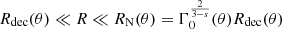 , and finally, to the Sedov-Taylor phase (Sedov 1946; Taylor 1950) in the non-relativistic regime for R ≫ RN(θ). For R ≫ Rdec(θ), the self-similar evolution becomes independent of the value of the initial Lorentz factor Γ0(θ).
When the Lorentz factor Γ(θ; R) and the velocity 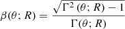 are known, the corresponding time t in the source frame is given by
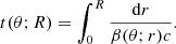
This leads to the solution R(θ, t) and Γ(θ, t) that we use for the dynamics of each component of the structured jet.
The physical conditions in the shocked medium are easily deduced from the shock-jump conditions in the strong-shock regime (Blandford & McKee 1976). In the comoving frame, the mass density equals

and the internal energy per unit mass is given by

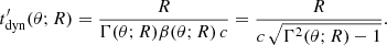
We assumed an adiabatic index of 4/3, which is valid as long as ϵ* ≫ c2. Finally, the timescale of the adiabatic cooling of the shocked region due to the spherical expansion is given in the comoving frame by
2.3. Accelerated electrons and amplified magnetic field
We consider a shocked region where the physical conditions in the comoving frame are given by the mass density ρ*, the internal energy per unit mass ϵ*, and the dynamical timescale t′dyn (i.e. the characteristic timescale of the adiabatic cooling due to the spherical expansion), and we assume that the emission is produced by non-thermal shock-accelerated electrons that radiate in a local turbulent magnetic field amplified at the shock. In practice, we only consider the forward external shock, so that in this study, ρ*, ϵ*, and t′dyn are given by Eqs. (14)–(16).
We use the following standard parametrisation of the microphysics at the shock: (i) a fraction ϵB of the internal energy is injected in the magnetic field,
leading to
(ii) a fraction ϵe of the internal energy is injected into non-thermal electrons that represent a fraction ζ of all available electrons. Their number density (cm−3) and energy density (erg ⋅ cm−3) in the comoving frame are therefore given by

and

We assume a power-law distribution at injection with an index −p and 2 < p < 3. This leads to the following distribution of accelerated electrons (cm−3):
where the minimum Lorentz factor at injection equals
As discussed below, it is important to take a realistic estimate of the maximum Lorentz factor γmax up to which electrons can be accelerated at the shock into account for a discussion of the GeV-TeV afterglow emission. This was not included in the study by Nakar et al. (2009), on which we base our calculation of the emission. Eqs. (21) and (22) above were obtained by assuming that the maximum Lorentz factor γmax is much higher than γm. This is fully justified as we have typically γmax/γm > 106 in the best-fit models of GW 170817 at the peak (Sect. 4). The maximum electron Lorentz factor γmax is evaluated by imposing that the acceleration timescale always remains shorter than the radiative and dynamical timescales,
The acceleration timescale is written as a function of the Larmor time R′L/c following Bohm’s scaling,
where Kacc ≥ 1 is a dimensionless factor. In practice, electrons at γmax usually cool fast, and the maximum electron Lorentz factor is determined by the radiative timescale, t′rad(γ). Its evaluation is non-trivial when IC scattering is taken into account (see Sect. 2.4). The resulting detailed calculation of γmax is explained in Appendix A. In the following, we assume Kacc = 1. Our value of γmax should therefore be considered as an upper limit for the true value of the maximum electron Lorentz factor.
2.4. Emissivity in the comoving frame
Our calculation of the emission from non-thermal electrons is mostly taken from Nakar et al. (2009). The population of electrons cools down by adiabatic cooling, synchrotron radiation, and via SSC scattering. As we are interested in the VHE afterglow emission, we include the attenuation due to pair production in Sect. 2.4.8, but do not include the emission of secondary leptons. We focus on the afterglow of GW 170817, for which the radio observations did not show any evidence for absorption, and we therefore do not include the effect of synchrotron self-absorption in the current version of the model. In this subsection, all quantities are written in the comoving frame of the considered shocked region. We therefore omit the prime to simplify the notations.
2.4.1. Synchrotron and inverse-Compton radiation for a single electron
2.4.1.1. Synchrotron radiation.
The synchrotron power of a single electron (erg ⋅ s−1) is given by
with  and KP a dimensionless parameter, and its synchrotron frequency equals
with  and Kν a dimensionless parameter. The dimensionless parameters KP and Kν depend on the assumptions made on the pitch angle of electrons relative to the magnetic field lines and different values are found in afterglow models, as listed in Table 1. By default, we use the same values as Gill & Granot (2018), taken from Granot et al. (1999), who obtained them by fitting the broken power-law approximation of the synchrotron power of a power-law distribution of electrons to the exact calculation.
Values of the dimensionless parameters KP; Kν and KPmax for different afterglow models used in each reference.
The corresponding synchrotron power at frequency ν (erg ⋅ s−1 ⋅ Hz−1) is given by
with
KPmax = KP/Kν and ∫0∞Φ(x)dx = 1. In practice, we adopt a simplified shape  for x ≤ 1 and 0 otherwise.
2.4.1.2. Inverse-Compton scattering.
The spectral number density of seed photons is nνsyn (cm−3 ⋅ Hz−1), which is assumed to result only from the synchrotron radiation of the electrons on which they also scatter (SSC). The IC power of an electron (erg ⋅ s−1) is then given by
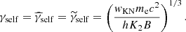
where w = γhν/mec2; and fKN and gKN are the KN corrections to the cross-section and to the mean energy of the scattered photon. In the Thomson regime (w ≪ wKN), the cross-section is σT and the mean energy of scattered photons is KIC γ2hν for a seed synchrotron photon with a frequency ν, so that fKN = gKN = 1 for w ≪ wKN. By default, we use the standard values KIC = 4/3 and wKN = 1, as in Nakar et al. (2009). We note, however, that Yamasaki & Piran (2022) recently suggested that a better agreement with a detailed numerical spectral calculation of the SSC component was achieved with wKN = 0.2, especially at the transition between the Thomson and the KN regime. For simplicity, we do not write in Eq. (29) the dependence on the angle between the upscattered photon and the scattering electron explicitly. This was discussed in Nakar et al. (2009). We assume an isotropic seed radiation field. We only account for single IC scattering as the effects of multiple scatterings are expected to be negligible because the afterglow is produced in the optically thin regime. The Compton parameter is defined by
This Compton parameter is constant only when SSC scattering occurs in the Thomson regime. We take the KN regime into account, which explains the dependence on the electron Lorentz factor. This affects not only the SSC emission, but also the synchrotron component. Following Nakar et al. (2009) and keeping the same notations, we simplify the IC cross-section by assuming that scattering is entirely suppressed in the KN regime: fKN(w) = 0 for w ≥ wKN. Then, a synchrotron photon produced by an electron with Lorentz factor γ can only be upscattered by electrons with Lorentz factors below a certain limit  to remain in the Thomson regime,
We note that  is a decreasing function of γ: If the energy of the synchrotron photon is higher, the maximum energy of any electron on which it could be upscattered in the Thomson regime must be lower. In an equivalent way, electrons with Lorentz factor γ only scatter photons below the energy
Then, it is convenient to define  such that
  ,
,
Electrons with a Lorentz factor γ can only scatter synchrotron photons produced by electrons with Lorentz factors below  . The Lorentz factor γself is defined by
The definition of  allows us to simplify the expression of the SSC power given by Eq. (29):
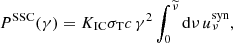
with uνsyn = nνsyn × hν the energy density of the seed synchrotron photons (erg ⋅ cm−3 ⋅ Hz−1). Then,
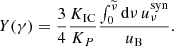
Assuming a strict suppression in the KN regime leads to a simple expression for the SSC power at frequency ν (erg ⋅ s−1 ⋅ Hz−1) for a single electron with a Lorentz factor γ,
if hν ≤ KICγmec2 and 0 otherwise.
2.4.2. Radiative regime of a single electron
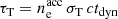
Following Sari et al. (1998), the first expected break in the electron distribution occurs at the critical electron Lorentz factor γc, defined by the condition trad(γ) = tdyn, so that high-energy electrons with γ ≫ γc are radiatively efficient (fast cooling), and low-energy electrons with γ ≪ γc mainly cool via the adiabatic expansion and are radiatively inefficient (slow cooling). The radiative timescale is given by
![$$ \begin{aligned} t_{\mathrm{rad} }(\gamma ) = \frac{\gamma m_{\mathrm{e} }c^2}{P_{\mathrm{syn} }(\gamma )+P_{\mathrm{SSC} }(\gamma )} = \frac{m_{\mathrm{e} }c^2}{\left[1+Y(\gamma )\right] K_1 B^2 \gamma }. \end{aligned} $$](/articles/aa/full_html/2024/10/aa47516-23/aa47516-23-eq57.gif)
Then, self-consistently computing γc requires us to solve the equation
![$$ \begin{aligned} \gamma _{\mathrm{c} } \left[1 + Y(\gamma _{\mathrm{c} })\right] = \gamma _{\mathrm{c} }^{\mathrm{syn} } = \frac{m_{\mathrm{e} }c^2}{K_1 B^2\, t_{\mathrm{dyn} }}, \end{aligned} $$](/articles/aa/full_html/2024/10/aa47516-23/aa47516-23-eq58.gif)
where  is the value of the critical Lorentz factor obtained when only the synchrotron radiation is taken into account. Our procedure to compute γc and Y(γc) in the most general case where the SSC cooling impacts the electron distribution is discussed below in Sect. 2.4.6.
2.4.3. Electron distribution and associated emission
2.4.3.1. Electron distribution.
Following Nakar et al. (2009), we compute the time-averaged distribution of electrons  over the dynamical timescale tdyn by keeping only the dominant term for the electron cooling: The instantaneous power of an electron is either dominated by the synchrotron and SSC radiation (1+Y(γ))Psyn(γ) for γ > γc or by the adiabatic cooling γ mec2/tdyn if γ < γc. This leads to
in fast-cooling regime (γm > γc) and to
in slow-cooling regime (γm < γc). We define γm, c = max(γm;γc) and γc, m = min(γm;γc) so that γm, c = γm and γc, m = γc in fast cooling and γm, c = γc and γc, m = γm in slow cooling. The minimum electron Lorentz factor therefore is γmin = γc, m. We define the corresponding synchrotron frequencies νm, c = νsyn(γm, c) and νc, m = νsyn(γc, m). We also always only keep the dominant term in the radiated power, that is, 1 + Y(γ)≃1 if Y(γ) < 1 and Y(γ) otherwise. As described in detail in Nakar et al. (2009), the resulting distribution shows several breaks in addition to γm and γc: A break is expected at γ0 such that Y(γ0) = 1, and several additional breaks are possible and must be identified in an iterative way, as described in Sect. 2.4.6.
Following Sari et al. (1998) and Nakar et al. (2009), we approximate  and the associated synchrotron spectrum by broken power laws to allow for a semi-analytical calculation. Electrons Lorentz factors are normalised by γm, c, that is, x = γ/γm, c, and photon frequencies by νm, c, that is, y = ν/νm, c. Hence, the normalised synchrotron frequency of an electron with normalised Lorentz factor x is y = x2. In the following, the notations introduced for characteristic electron Lorentz factors or photon frequencies are implicitly conserved for the normalised quantities. For instance, xself = γself/γm, c,
  , and
, and  .
.
2.4.3.2. Normalised electron distribution.
The electron distribution is given by
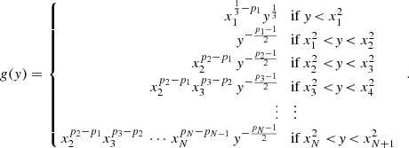
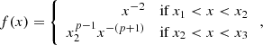
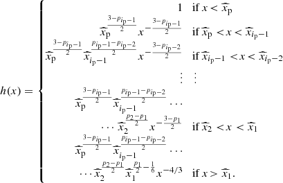
where f(x) is the normalised broken power-law electron distribution with N breaks and power-law segments,
with x1 = γmin/γm, c and xN + 1 = γmax/γm, c. The number of breaks in the purely synchrotron case or when all IC scatterings are in the Thomson regime is N = 2, as discussed in Sect. 2.4.4 and 2.4.5. In the general case, where KN corrections cannot be neglected, more breaks appear in the electron distribution, as discussed in Sect. 2.4.6. All possible cases are provided in Appendix B. Typically, N = 2 to 5, except in some very specific regions of the parameter space (case III in Nakar et al. 2009). This is also discussed in Appendix B.
The dimensionless integral I0 is given by
to conserve the number of electrons,  .
.
2.4.3.3. Normalised synchrotron spectrum.
The synchrotron power per electron and per unit frequency pνsyn (erg ⋅ s−1 ⋅ Hz−1 ⋅ electron−1) averaged over the timescale tdyn is deduced from Eq. (27) using the simplified shape for Φ. This leads to a broken power-law synchrotron spectrum,
where the normalised broken power-law spectral shape is obtained by keeping the dominant term in the integral of f(x)/x2/3,
The dimensionless factors I2 and J0 are defined by
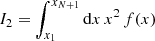
to ensure that the total synchrotron power per electron (erg ⋅ s−1 ⋅ electron−1) is conserved,
Finally, we define νp as the peak frequency of the synchrotron spectrum, that is, the frequency ν where ν2pνsyn is maximum. This peak frequency corresponds to synchrotron photons emitted by electrons at a Lorentz factor γp, that is, νp = νsyn(γp). We note ip the corresponding index of the break in the normalised distributions: xp = xip and yp = yip = xp2.
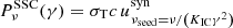
2.4.3.4. Normalised SSC spectrum.
The SSC power per electron and per unit frequency pνSSC (erg ⋅ s−1 ⋅ Hz−1 ⋅ electron−1) emitted over the timescale tdyn is deduced from Eq. (37) with
This leads to
where
is the Thomson optical depth, and where the normalised spectral shape is given by
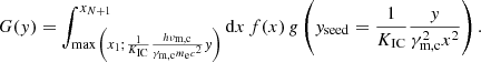
The cutoff at xKN = γKN/γm, c with 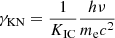 is a direct consequence of the strict suppression assumed in the KN regime: The VHE flux due to the scattering in the KN regime is neglected. Yamasaki & Piran (2022) introduced a factor fKN in their calculations to compensate for this approximation, which we do not include here. The KN regime affects the high-energy part of the emitted spectrum: Above a photon energy hν = KICγminmec2, we have γKN > γmin and the SSC emission is reduced. The SSC emission is even entirely suppressed (G(y) = 0) at very high photon energies hν > KICγmaxmec2, corresponding to γKN > γmax.
In practice, G(y) is computed exactly in our numerical implementation. We also note that J0 ≃ 2I2 when only the leading term is kept in the integrals. However, all dimensionless factors I0, I2, and J0 are also computed exactly in our numerical implementation, which ensures the continuity of the electron distribution and emitted spectrum at the transition from the fast- to the slow-cooling regime, as well as between the different possible cases in either regime (see Sect. 2.4.6).
2.4.4. Purely synchrotron case
The standard purely synchrotron case in which the SSC emission is neglected (Y(γ) = 0 for all electrons) was fully described in Sari et al. (1998). We have γc = γcsyn in this case. In the fast-cooling regime (γm > γc), the normalised distributions are given by
with x1 = γc/γm, x2 = 1 and x3 = γmax/γm. In the slow-cooling regime (γm < γc), they are given by
with x1 = γm/γc, x2 = 1 and x3 = γmax/γc. Calculations using this prescription are labelled “no SSC” in the following.
2.4.5. Synchrotron self-Compton case in the Thomson regime
If the KN regime is neglected, all IC scatterings occur in the Thomson regime, and the Compton parameter is the same for all electrons: Y(γ) = Yno KN = cst. The corresponding solution was given by Sari & Esin (2001): The normalised distributions f(x) and g(y) are the same as in the purely synchrotron case above, but the value of the critical Lorentz factor γc is decreased due to the IC cooling, γc = γcsyn/(1+Yno KN). Using Eqs. (36), (46), and (51), we obtain
As I2/I0 is a function of γc/γm = γcsyn/γm/(1 + Yno KN), this is an implicit equation to be solved numerically to obtain Yno KN and γc. The limits for (1+Yno KN)Yno KN are  for γm ≫ γc and
 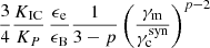 for γm ≪ γc. Calculations using this prescription are labelled “SSC (Thomson)” in the following.
2.4.6. Self-consistent calculation of the electron distribution and the Compton parameter in the general case
2.4.6.1. Normalised Compton parameter.
In the general case where the KN suppression at high energy is included, the Compton parameter Y(γ) is a decreasing function of the electron Lorentz factor. From Eqs. (36), (46), and (51), we obtain
For low Lorentz factors γ,  becomes very large, so that for
  , we recover the Thomson regime, where the right-hand side of Eq. (61) is formally the same as in Eq. (60), even if the integrals I0 and I2 can be different when the normalised electron distribution f(x) is different. As described in Nakar et al. (2009), when only the leading term in the integral of g(y) is kept, the corresponding scaling law for the Compton parameter is Y(γ) = cst if
  is above the peak frequency νp and
  otherwise, where
  is the slope of electron distribution in the power-law segment of the electron distribution including
  . We therefore introduce a normalised Compton parameter defined by
where h(x) follows this scaling and is normalised so that Eq. (62) has the exact limit in the Thomson regime. This leads to
We recall that ip is the index of the break corresponding to the peak frequency of the synchrotron spectrum. In most cases (see Appendix B), we have ip = 2, leading to
2.4.6.2. Self-consistent solution for the normalised electron distribution.
Following Nakar et al. (2009), we define2γ0 by Y(γ0) = 1 and assume 1 + Y(γ) = Y(γ) for γ < γ0 and 1 otherwise. From Eqs. (40) and (41), this shows that the IC cooling only affects the electron distribution in the interval
Therefore, the solution is entirely determined by the orderings of γm, γc, γ0,  , and
, and  . All possible cases and the corresponding solutions are listed in Appendix B. In some cases, subcases are introduced as breaks can appear at
  ,
,  ,
,  , etc. All the most relevant cases for GRB afterglows were described in Nakar et al. (2009), along with the detailed method for obtaining the corresponding solution for the electron distribution. For completeness, we list in Appendix B the additional cases that allow us to fully describe the parameter space, even in regions that are unlikely to be explored in GRBs.
2.4.6.3. Calculation of the critical Lorentz factor γc.
From Eq. (62), we obtain the following equation for Y(γc):
where  is a constant as the microphysics parameters ϵB, ϵe, and p are assumed to be constant during the forward-shock propagation. We note that xc = 1 in the slow-cooling regime γm < γc. A second useful relation is obtained from Eq. (62) and the definition of γ0,
Then, γc is computed from the following implicit equation, which is solved iteratively,
We start by assuming Y(γc) = Yno KN as defined in Sect. 2.4.5 and then iterate as follows:
-
Compute γc from Eq. (68).
-
Knowing γm, γc, and γself, scan the different possible cases for the ordering of γm, γc, γ0,
 , and
, and  (and additional characteristic Lorentz factors for some cases) as listed in Appendix B and compute γ0 from Eq. (67), which can be analytically inverted as provided for each case in Appendix B. We stop the scan of the possible cases when the ordering of all characteristic Lorentz factors including the obtained value of γ0 is the correct one.
 -
Having identified the correct case and therefore knowing the expression of f(x), compute the integrals I0 and I2.
-
Compute an updated value of Y(γc) from Eq. (66).
-
Start a new iteration at step 1 until convergence.
We stop the procedure when the relative variation of γc in an iteration falls below ϵtol. We use ϵtol = 10−4, which is reached in most cases in fewer than 20 iterations. In the context of a full afterglow light-curve calculation, as we expect Y to vary smoothly during the jet propagation, we use the value of Y(γc) obtained at the previous step of the dynamics instead of Yno KN to start the iterative procedure. Then, we usually reach convergence in only a few iterations.
2.4.7. Final calculation of the emission in the comoving frame
The self-consistent spectrum in the comoving frame, that is, pνsyn and pνSSC, the synchrotron and SSC powers per electron and per unit frequency averaged over the timescale tdyn, can be computed by the following procedure based on the previous paragraphs:
-
The input parameters are
 , tdyn, B, ue/uB = ϵe/ϵB, γm, and p.
 -
The following quantities can immediately be deduced: γcsyn from Eq. (39), γself from Eq. (34), τT from Eq. (54), and Yno KN from Eq. (60).
-
Then, the iterative procedure described above allows us to identify the spectral regime among all the possibilities listed in Appendix B, and we can compute γc. At the end of this step, all breaks and slopes in the functions f(x) and h(x) are known. The corresponding integrals I0 and I2 are computed by a numerical integration of Eqs. (44) and (48).
-
The function g(y) can immediately be deduced from f(x), using Eq. (47). The corresponding integral J0 is computed by a numerical integration of Eq. (49), and the synchrotron spectrum per electron, pνsyn, is deduced from Eq. (46).
-
Finally, the function G(y) is computed by an numerical integration of Eq. (55) and the SSC spectrum per electron, pνSSC, is deduced from Eq. (53).
2.4.8. Pair production
At VHE, pair production  can start to contribute to the SSC flux depletion. We account for this mechanism by a simplified treatment, assuming an isotropic distribution of the low-energy seed photons, as for the SSC calculation, and approximating the cross-section for pair production by a Dirac function at twice the threshold of the interaction. Then, VHE photons of frequency ν can produce pairs by interacting with low-energy photons at a frequency νseed = 2(mec2)2/(h2ν), and the characteristic timescale of this interaction is given by
![$$ \begin{aligned} t_{\gamma \gamma }(\nu ) = \frac{h}{\sigma _{\rm T}c} \left[ u_{\nu _\mathrm{seed} =2\frac{\left( m_\mathrm{e} c^2\right)^2}{h^2 \nu }} \right]^{-1}, \end{aligned} $$](/articles/aa/full_html/2024/10/aa47516-23/aa47516-23-eq112.gif)
with uν = uνsyn + uνSSC = neacc(pνsyn+pνSSC)tdyn, leading to
![$$ \begin{aligned} t_{\gamma \gamma }(\nu ) = \frac{h}{\tau _{\rm T}} \left[ \left(p_{\nu _\mathrm{seed} }^\mathrm{syn} +p_{\nu _\mathrm{seed} }^\mathrm{SSC} \right)_{\nu _\mathrm{seed} =2\frac{\left( m_\mathrm{e} c^2\right)^2}{h^2 \nu }} \right]^{-1}. \end{aligned} $$](/articles/aa/full_html/2024/10/aa47516-23/aa47516-23-eq113.gif)
For very high frequencies ν, the seed photons for pair production have a low frequency and pνseedsyn + pνseedSSC ≃ pνseedsyn. The total emitted power per electron pν = pνsyn + pνSSC is then corrected for by a factor 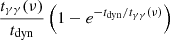 , which in practice only attenuates the SSC component at high frequency, where tγγ(ν)≪tdyn.
The implementation of the model allows us to select the level of approximation for the SSC emission (synchrotron only, Thomson, or full calculation) and to include or exclude the attenuation due to the pair production.
2.5. Observed flux
When the emissivity in the comoving frame is known (Sect. 2.4), the flux measured by a distant observer with a viewing angle θv is computed by an integration over equal-arrival time surfaces, taking into account relativistic Doppler boosting and relativistic beaming, as well as the effect of cosmological redshift. This leads to the following expression of the observer frame flux density (erg ⋅ s−1 ⋅ cm−2 ⋅ Hz−1) measured at time tobsz and frequency νobsz(Woods & Loeb 1999):
![$$ \begin{aligned} F_{\nu _{\rm obs}^z}\left(t_{\rm obs}^z\right)&= \frac{1 + z}{4\pi D_{\rm L}^2} \int _0^{\infty }\mathrm{d} {r}\, \int _0^{\pi }\mathrm{d} \psi \,\int _0^{2\pi }\mathrm{d} {\phi }\, r^2 \sin {\psi }\\\nonumber&\!\!\!\!\!\!\times \left[\mathcal{D} ^2(r,\psi ,t)\, 4\pi j^{\prime }_{\nu ^{\prime }}\left(r,\psi , \phi ,t\right)\right]_{t=\frac{t_{\rm obs}^z}{1+z}+\frac{r}{c}\cos {\psi }}, \end{aligned} $$](/articles/aa/full_html/2024/10/aa47516-23/aa47516-23-eq115.gif)
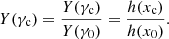
where we use spherical coordinates (r;ψ;ϕ) with the polar axis equal to the line of sight, ψ and ϕ the colatitude and longitude, and the jet axis in the direction (ψ=θv,ϕ = 0) (see Fig. 1), and where z and DL are the redshift and the luminosity distance of the source. The angle ψ differs from θ used in Sect. 2.2, which is measured from the jet axis. The time t (source frame) and frequency ν′ (comoving frame) are given by

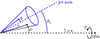 |
Fig. 1. Coordinates and notations used in the expression of the observed flux. |
The Doppler factor is expressed as
and j′ν′ is the emissivity (erg ⋅ cm−3 ⋅ s−1 ⋅ Hz−1 ⋅ sr−1) in the comoving frame.
In practice, following the discretisation of the jet structure described in Sect. 2.1, the observer-frame flux density Fνobsz(tobsz) is computed as  , where Fνobsz(i)(tobsz) are the contributions of the core jet (i = 0) and lateral rings (i = 1 → N). To compute each contribution, the thin-shell approximation allows us to reduce the double integral over r and ψ in Eq. (71) to a simple integral over r, or equivalently, over ψ or t. In addition, to improve the computation time, the remaining integral on ϕ is computed analytically. This leads to
![$$ \begin{aligned} F_{\nu _{\rm obs}^z}^{(i)}\left(t_{\rm obs}^z\right) \!\!\!&= \!\!\!\frac{1+z}{4\pi D_{\rm L}^2} \int \limits _{t_{\mathrm{min} }^{(i)}(t_{\rm obs}^z)}^{t_{\mathrm{max} }^{(i)}(t_{\rm obs}^z)} \!\!\!\! \frac{c\, \mathrm{d} t}{2\Gamma _i(t)R_i(t)}\, \frac{\Delta \phi _i\left(\theta _\mathrm{v} ;\psi _i(t^z_\mathrm{obs} ;t)\right)}{2\pi }\nonumber \\&\times \mathcal{D} _i^2\left(t^z_\mathrm{obs} ;t\right)\, \left[ 4\pi N_\mathrm{e} \left(R_i(t)\right)\right]\, p^{\prime (i)}_{\nu ^{\prime }}(t), \end{aligned} $$](/articles/aa/full_html/2024/10/aa47516-23/aa47516-23-eq120.gif)
where
Ne(r) = ζMext(r)/mp is the number of shock-accelerated electrons per unit solid angle, and p′ν′(i)(t) is the power per unit frequency and per electron in the comoving frame computed in Sect. 2.4 and evaluated at time t and comoving frequency ν′=(1 + z)νobsz/𝒟i(tobsz;t).
The limits of the integral  and
and  are defined by the condition ψmin, i ≤ ψi(tobsz;t) ≤ ψmax, i, where
and ψmax, i = θv + θmax, i, that is,
Finally, we use the exact analytical calculation of the geometrical term Δϕi defined by Δϕi(θv; ψ) = ∫02πdϕfi(θv; ψ; ϕ), where fi(θv; ψ; ϕ) = 1 when the direction (ψ;ϕ) is contained in the component i (core jet or ring) and 0 otherwise.
3. Comparison with other afterglow models
3.1. Dynamics and synchrotron emission
To test our calculation of the dynamics of the forward external shock and the associated synchrotron emission, we compared our results with two other models of the afterglow of a structured jet: the model presented in Gill & Granot (2018), and afterglowpy, a public Python module for calculating GRB afterglow light curves and spectra, based on Ryan et al. (2020).
The first comparison is straightforward: With our default values of the normalisation coefficients Kν and KP, the assumptions (dynamics, microphysics, radiation, calculation of observed quantities) of our model in the purely synchrotron case are exactly the same as in Gill & Granot (2018). We verified that we exactly reproduced the different cases in their Fig. 4.
The case of afterglowpy requires a more detailed comparison as there are differences in some treatments of the afterglow physics.
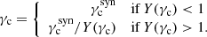
(1) Early dynamics: In afterglowpy, even the early-time dynamics is computed assuming the self-similar Blandford & McKee regime, that is, Γ(t; θ)∝E(θ)1/2n01/2t−3/2 (see Sect. 2.1 in Ryan et al. 2020), whereas we included the coasting phase with Γ ∼ cst before a smooth transition towards the self-similar regime at the deceleration radius, as described in Sect. 2.2. Fig. 2 compares for a typical set of parameters the afterglow light curves from a top-hat jet viewed on-axis in radio, optical, and X-rays obtained with our model (solid line), afterglowpy (dashed line), and our model where the dynamics was forced to be in the self-similar regime at all times (dotted line). This allows us to confirm that the two models with the same self-similar dynamics agree well, except for the flux normalisation, as discussed below, and that the model with the full dynamics progressively converges towards the same solution: Following the peak at the deceleration radius (at ∼10−2 days in this example), the light curve obtained with the full dynamics smoothly converges towards the self-similar solution, and the two light curves are identical at late times (typically after the jet break at ∼2 days in this example). On the other hand, the self-similar approximation strongly over-estimates the fluxes until the deceleration radius, and the full dynamics should always be included when considering early observations (see also Wang et al. 2024). In the case of GW 170817 discussed in the next section, the earliest detection by Chandra was obtained ∼9 days after the merger, by which time, the core jet dynamics had reached the self-similar regime.
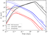 |
Fig. 2. Synthetic afterglow light curves of a top-hat jet viewed on-axis in the synchrotron-only radiation regime. The solid lines show the results obtained using our model with full dynamics treatment (using Eq. (10)). The dotted lines follow the self-similar solution at all times. The dashed lines are obtained with afterglowpy without lateral expansion. The fluxes are computed in radio at 3 GHz (black), in optical in r band at 5.06 × 10¹⁴ Hz (blue), and in X-rays at 1 keV (red). The parameters used for this figure are E0, iso = 1052 erg, θc = 4 deg, next = 10−3 cm−3, ϵe = 10−1, ϵB = 10−1, p = 2.2, and DL = 100 Mpc. |
(2) Late dynamics: In contrast to afterglowpy, the current version of our model does not include lateral expansion of the ejecta. When we compared it with afterglowpy, we therefore deactivated this option in the latter, which led to the excellent late-time agreement shown in Fig. 2. The impact of the lateral spreading is expected to be very limited as long as the core jet is relativistic (see e.g. Woods & Loeb 1999; Granot & Piran 2012; van Eerten & MacFadyen 2012; Duffell & Laskar 2018), so that we stopped the jet propagation when the core Lorentz factor reached Γ = 2 in the simulations of the afterglow of GW 170817 discussed in the next section. In addition, we excluded observations after 400 days from the data set used for the afterglow fitting, which corresponds to Γ ≳ 3 − 4 for the core jet in our best-fit models.
(3) Flux normalisation: afterglowpy relies on a scaling to boxfit (van Eerten et al. 2012), while in our model, this normalisation is derived from analytical approximations detailed in Sect. 2. This leads to the difference in the normalisation shown in Fig. 2 when afterglowpy is compared with our model, where the same self-similar dynamics is forced. The flux ratio varies between 1 and 5 at all wavelengths. When exploring a broad parameter space, varying the angle, energy injection, and microphysical parameters, we verified that the flux ratio never exceeded 5.
To conclude this comparison, we note that afterglowpy and our model (in purely synchrotron mode) have been used by Kann et al. (2023) for two independent Bayesian inferences of the parameters of the afterglow of GRB 221009A using the same set of early observational data. The two codes converged towards very similar solutions.
3.2. Synchrotron self-Compton emission
We now test the predictions of our model in the SSC regime. Several GRBs have been observed at VHE. Two events were particularly well followed up at all wavelengths, GRB 190114C (MAGIC Collaboration 2019a,b) and GRB 221009A (LHAASO Collaboration 2023). In both cases, the VHE detection occurred at very early times, but the analysis favoured a dominant external forward-shock origin for the emission. However, the case of GRB 221009A, which is an extreme GRB (the brightest ever detected by far) is quite complex. According to several studies, the early VHE emission and the later observations at lower frequencies probe different regions of a structured jet seen on-axis and may also include a significant contribution of the reverse shock at some frequencies (see e.g. Laskar et al. 2023; O’Connor et al. 2023; Gill & Granot 2023; Sato et al. 2023; Zheng et al. 2024; Zhang et al. 2024; Derishev & Piran 2024). We therefore decided to rather focus on GRB 190114C to test our model. This long GRB has rich observational follow-up from radio to VHE at simultaneous times. Following MAGIC Collaboration (2019a), we assumed that the spectrum shows two distinct components.
To test the radiative component of our model independently of the dynamics, we decided to analyse the observed spectrum at one fixed time, tobs = 90 s, following the approach proposed by Yamasaki & Piran (2022). Their spectral model was also based on Nakar et al. (2009), which allows an easy comparison. For this purpose, we used their values KIC = 1 and wKN = 0.2 in this subsection. We also considered a one-zone model of the emitting region, characterised by a radius R, a Lorentz factor Γ, and Ne accelerated electrons radiating in a magnetic field B′. The electrons were injected with an initial distribution with a minimum Lorentz factor γm and a slope p. Following Yamasaki & Piran (2022), we fixed p = 2.5 and let four parameters free for the spectral fitting: Γ, B′, γm, and ϵe/ϵB. Then, R and t′dyn were deduced from Γ and tobs, neacc from B′, ϵe/ϵB, γm, and p, and finally, Ne from neacc, R, and Γ (see Sect. 2 in Yamasaki & Piran 2022).
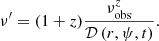
We used the same observational data as Yamasaki & Piran (2022), shown in black in Fig. 3. We then fit the data using an MCMC procedure with log-uniform priors, such that 1.3 < logΓ < 3.5; 0 < log ϵe/ϵB < 4; −2 < log B < 3; 1 < log γm < 7.
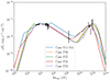 |
Fig. 3. Spectral fits to the afterglow observations of GRB 190114C at 90 s (black data points taken from MAGIC Collaboration 2019b). Each colour represents the best-fit spectrum for each of the possible radiative regimes (see text and Fig. 4). The spectral cases are detailed in Appendix B. This figure can be compared to Fig. 6 in Yamasaki & Piran (2022), which shows very similar fits. |
The marginalised posterior distributions for these four parameters are provided on the first row of Fig. 4. As also discussed in Yamasaki & Piran (2022), several spectral solutions are possible. We show for the further discussion the posterior distributions of  , γc/γm, and B/Γ3, as well as the distribution of spectral cases in the bottom row of Fig. 4. The best-fit model for each of the spectral cases is shown in Fig. 3. We find a high overall agreement with the results of Yamasaki & Piran (2022).
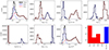 |
Fig. 4. Marginalised posterior distributions for the spectral fit of the afterglow observations of GRB 190114C at tobs = 90 s. The total (black) is subdivided between the slow (blue) and fast (red) cooling cases. The first row shows the four free parameters explored in this MCMC analysis (Γ, ϵe/ϵB, B and γm). In the second row, we show some derived quantities: |

-
The identified radiative regimes in the best-fit models are the same: Cases F24 and F25 correspond to their cases IIc and III (top row in their Fig. 6), F26 and F27 to their case I (middle row in their Fig. 6), and S11-S14 to one subcase of their slow case I (bottom right panel in their Fig. 6).
-
Most best models are in fast cooling (see the distribution of γc/γm in Fig. 4), with electrons at γm close to the transition between the Thomson and the KN regimes (see the distribution of
 in Fig. 4).
 -
The peak of the posterior distributions of ϵe/ϵB and γm in Fig. 4 is very close to the assumed values in their Fig. 6 (as indicated by the vertical dotted black lines).
-
Based on the analytical estimates from Derishev & Piran (2021), Yamasaki & Piran (2022) assumed a strong correlation between the Lorentz factor and the magnetic field with B/Γ3 ∼ 10−7. Our MCMC exploration confirms this result, but gives an estimate of the dispersion (see the distribution of B/Γ3 in Fig. 4).
A detailed comparison shows that our results differ slightly for the exact parameter values, owing to some differing normalisation constants. It should therefore be kept in mind that the absolute parameter values from spectral fits from different GRB afterglow studies should only be compared when the models that were used are the same.
The good agreement of our results with Yamasaki & Piran (2022) allows us to validate our radiative model, as both studies are independent implementations of the synchrotron+SSC model using the same level of approximation. In addition, we confirm that this model is a convincing candidate to reproduce the broadband emission of GRB 190114C.
4. Very high energy afterglow of GW 170817
Having validated the calculation of the dynamics and synchrotron + SSC emission in our model, we now present the results obtained by fitting the observations of the GRB afterglow of GW 170817 using a Bayesian analysis.
4.1. Observational data
In its numerical implementation, our model allows for simultaneous multi-wavelength modelling. We used 94 data points, from radio to X-rays between 9.2 and 380 days3, as compiled and reprocessed homogeneously by Makhathini et al. (2021). We also included the five constraining early-time upper limits also reported in Makhathini et al. (2021), as shown in Table 2. Early-time constraints are useful to restrict the posterior models to those with a single peak in flux density, as discussed in Sect. 2.2. All these flux measurements and upper limits were fitted simultaneously.
Early-time upper limits used in the afterglow fitting.
The likelihood that we used for our study is based on a modified χ2 calculation to account for the upper limits,
![$$ \begin{aligned} \ln {\mathcal{L} } = - \frac{1}{2}\, \left[ \sum _{i} \frac{\left(m_i - d_i\right)^2}{\sigma _i^2} \!+\! \sum _{j} \frac{\left(\max {\{ u_j; m_j \}} - u_j \right)^2}{\sigma _j^2} \right], \end{aligned} $$](/articles/aa/full_html/2024/10/aa47516-23/aa47516-23-eq130.gif)
where the first sum concerns observational data (subscripts i), while the second sum concerns upper limits (subscripts j). The quantities mi and mj are the model flux densities at each observing time and frequency of the observational data set, di is the flux density value of a detection, σi is its associated uncertainty, uj is the upper flux limit presented in Table 2, and σj is an equivalent uncertainty that we arbitrarily defined as σj = 0.2uj, which roughly corresponds to the typical uncertainties for the detections. Adding this element accounts for some models whose predictions are slightly above the reported upper limit. The quantity max{uj; mj} in the second term implies that it behaves as a penalty that is only added for predicted fluxes mj above the observed upper limits. Another option would be to force the likelihood to diverge as soon as one of the modelled fluxes is above the corresponding upper limit.
We chose to exclude late-time observations after 400 days in the fits. We expect the lateral spreading of the jet to play a role at late times, when the shock front reaches Lorentz factors Γ ≲ 3, by which point our model no longer accurately describes the jet dynamics. In addition, other emission sites (e.g. the kilonova afterglow; Nakar & Piran 2011) could also contribute to the observed flux at late times. It is also difficult to include the latest observations (Hajela et al. 2022), which were not included in the compilation by Makhathini et al. (2021): Late-time data in X-rays consist of only a few photons, and a correct modelling in this case should be expressed in photon counts and should account for the instrumental response and low-statistics effects. The result of such an analysis is currently unclear, with an uncertain late rebrightening (Hajela et al. 2022) (see the discussion in Troja et al. 2022). An interpretation of the late evolution of the afterglow of GW 170817 appears to require a dedicated study, and we therefore excluded this phase from the analysis presented here. Finally, we did not include the H.E.S.S. upper limit at the peak (Abdalla et al. 2020), or the Fermi large area telescope (LAT) and H.E.S.S. early upper limits (Ajello et al. 2018; Abdalla et al. 2017), as they do not constrain the fit (see Sect. 4.4).
4.2. Results from the afterglow fitting
We performed a Bayesian analysis of the afterglow data of GW 170817 using the Markov chain Monte Carlo (MCMC) algorithm of the Python suite emcee (Foreman-Mackey et al. 2013, 2019). We ran three separate fits that differed only in the assumptions for the radiative processes in the shocked region.
-
“no SSC”: Emission is only produced by synchrotron radiation, as described in Sari et al. (1998) and Sect. 2.4.4.
-
“SSC (Thomson)”: SSC is taken into account assuming that all scatterings occur in the Thomson regime, as described in Sari & Esin (2001) and Sect. 2.4.5.
-
“SSC (with KN)”: SSC is taken into account including the KN regime, as described in Nakar et al. (2009) and Sect. 2.4.6.
The priors used for these three fits are identical and presented in Table 3. We used (log-)uniform priors over large intervals in order to remain as agnostic as possible. Their bounds are shown in Table 3. Additional constraints on the viewing angle can be obtained by combining the GW signal and the accurate distance and localisation of the host galaxy (Finstad et al. 2018), or by combining the afterglow photometry and VLBI imagery (Govreen-Segal & Nakar 2023), and the density of the external medium can be constrained from direct observation of the host galaxy (Hallinan et al. 2017; Hajela et al. 2019). We did not include them to focus on the constraints obtained from the afterglow modelling alone.
Free parameters of the MCMC and their prior bounds and shape.
For each of the three fits, we initialised 50 chains and ran 10 000 iterations per chain. After studying the convergence speed, we removed the first 2000 iterations for each chain. We show the posterior distributions for the remaining 400 000 parameter samples.
We present the marginalised posterior distribution of the free parameters for the three fits in Fig. 5, complemented by Fig. C.1, which shows the corresponding joint and marginalised posterior distributions at 3σ credibility (corner plot). We also show in Fig. 5 the distribution of some derived quantities, the true initial kinetic energy of the ejecta E0 as deduced from Eq. (5), the ratio of the viewing angle over the opening angle of the core jet θv/θc, and the four conditions for single-peaked light curves described by Beniamini et al. (2020b) and in Sect. 2.2. The three fits lead to similar distributions across the parameter space, with a few exceptions that are discussed in Sect. 4.3. The median parameter values as well as their 90% credible intervals are reported in Table 4. We finally show in Table 5 the median values of the derived quantities shown in Fig. 5.
Posterior values for the free parameters of the three fits of the afterglow of GW 170817.
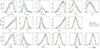 |
Fig. 5. Comparison of the marginalised posterior distributions for the three fits of the afterglow of GW 170817 presented in Sect. 4, which differ only by the treatment of the radiative processes: “no SSC” in blue; “SSC (Thomson)” in green; “SSC (with KN)” in orange. The first two rows show the inferred distributions of the free model parameters. The last row shows the distributions of several quantities derived from these parameters: The true energy of the jet E0 (see Eq. (5)), the ratio θv/θc, and the four quantities used in the conditions for single-peaked light curves from Beniamini et al. (2020b) and described in Sect. 2.2, log(θcΓ0c), 8b/a, |

Posterior values for several derived quantities from the three fits of the afterglow of GW 170817.
The detailed joint posterior distributions for the “SSC (with KN)” model where emission is produced by synchrotron radiation and SSC scatterings in the Thomson and KN regimes are shown in Fig. 6. In this figure, which is representative of the results obtained with the three fits, we observe typical correlations between some of the afterglow parameters, such as θc and θv, E0, isoc and next, or ϵe and ϵB. Some other parameters are anti-correlated, such as E0, isoc and ϵB, or next and ϵB. These degeneracies in the model parameters are expected when only the synchrotron component is observed (see e.g. Aksulu et al. 2022). In the case of GW 170817, the afterglow light curves can to first approximation be described by five quantities: its peak time, peak flux, the temporal slopes of the rising and decreasing phase, and the spectral slope. This does not allow us to constrain all the free parameters listed in Table 3.
 |
Fig. 6. Posterior joint and marginalised distributions of the free model parameters, E0, isoc, θc, θv, next, ϵB, ϵe, ζ, pa, Γ0c, b, for the “SSC (with KN)” fit of the afterglow of GW 170817 presented in Sect. 4, which includes SSC scatterings in the Thomson and KN regimes. The priors are all uniform or log-uniform and are shown in Table 3. The fitted data include all points until tmax = 400 days, as well as five early-time upper limits (see Sect. 4.1). The coloured contours correspond to the 1σ, 2σ, and 3σ confidence intervals for each parameter. |
As a post-processing step, we resampled 20 000 light curves at several observing frequencies (3 GHz, 1 keV, and 1 TeV) and spectra at several observing times (20 days, 110 days, and 400 days), where the set of parameters was directly drawn from the posterior sample for each of the three fits. At each observing time (for the light curves) or at each frequency (for the spectra), we then determined the 68% and 97.5% credible intervals for the distribution of predicted flux densities, which we used to draw confidence contours around the median value of the light curves and spectra. Because the posterior samples are similar for the three models, we only show the results for the most realistic case (“SSC (with KN)” model) in Figs. 7 and 8 (radio and VHE light curve), and in Fig. 9 (spectrum at 110 days, close to the peak).
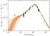 |
Fig. 7. Posterior distribution of the radio light curves at νobs = 3 GHz for the “SSC (with KN)” fit of the afterglow of GW 170817. The solid lines represent the median value at each observing time, the dark contours are the 68% confidence interval, and the light contours show the 97.5% confidence interval. Late-time observations that were not used in the fit are shown in blue. |
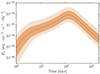 |
Fig. 8. Posterior distribution of the VHE light curves at hνobs = 1 TeV for the “SSC (with KN)” fit of the afterglow of GW 170817. Same as in Fig. 7. This is a prediction of the model. No observational constraint is included in the fit. |
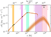 |
Fig. 9. Posterior distribution of the afterglow spectrum around its peak (tobs = 110 days) for the “SSC (with KN)” fit of the afterglow of GW 170817. The data points show the multi-wavelength observations at tobs ± 4 days. The upper limit from H.E.S.S. is also indicated (Abdalla et al. 2020). The low-energy component (solid line) is produced by synchrotron radiation, while the high-energy emission (dashed line) is powered by SSC scattering. The thick lines represent the median value at each observing frequency, the dark contours show the 68% confidence interval, and the light contours present the 97.5% confidence interval. Some instrument observing spectral ranges are shown in colours. |
4.3. Discussion: Inferred parameters
As shown in Fig. 7, the afterglow of GW 170817 is very well fitted by the model. The model accurately predicts the flux at all times, with a very small dispersion. The dispersion of the predicted flux is larger at very early or very late times, when no data point is included in the fit. The quality of the model prediction is the same for the spectrum in Fig. 9. The frequency νm, obs is below the data points at the lowest frequency, with some dispersion in absence of observational constraints. The critical frequency νc, obs is found to be in X-rays, just above the highest-frequency data points.
The inferred values of most model parameters (Fig. 5 and Table 4) are very similar to the results obtained in previous studies that modelled the same afterglow with the synchrotron radiation from a decelerating structured jet (Troja et al. 2019; Lamb et al. 2019; Ghirlanda et al. 2019; Ryan et al. 2020), with some exceptions that are due to different priors. A first difference concerns the viewing and core jet opening angles θv and θc. Even though the values inferred by the “SSC (with KN)” fit are comparable with values found in previous studies, the corresponding ratio θv/θc ∼ 11 (Table 5) is at the higher end of the other predictions. Nakar & Piran (2021) reported a compilation of these predictions and showed that afterglow light curves can only constrain this ratio and not the two parameters independently, which is confirmed by the correlation observed in Fig. 6. This difference is probably due to the flat and broad priors we used for these two parameters, whereas most previous studies used much stricter priors based on an external constraint, either on the viewing angle derived from GW data using the value of the Hubble constant from Planck (as in Troja et al. 2019; Ryan et al. 2020), or a constraint on the viewing angle and the core jet using VLBI imagery (as in Ghirlanda et al. 2019; Lamb et al. 2019). The marginalised distributions of θv and θc show that a restricted region of the parameter space has been explored by the MCMC chains for these parameters, as is also visible in Fig. C.1.
When compared with the results of Ryan et al. (2020), whose assumptions are closest to those of our “no SSC” fit and who computed the light curves using afterglowpy, with which we compared our model in Sect. 3, we also find that our predicted values for E0,isoc and next are higher by about one order of magnitude. Fig. 6 shows that it is also an effect of our different priors for the angles. However, we observe that the expected strong correlation between these two parameters and the inferred ratio E0, isoc/next ∼ 1055 erg ⋅ cm−3 (Table 5) is close to the value obtained by Ryan et al. (2020). Using similar priors for the angles, or including a constraint on the external density from the observation of the host galaxy (Hallinan et al. 2017; Hajela et al. 2019), would then reduce the inferred values for these two parameters. We discuss below the fact that detections in the VHE range would help us to break this degeneracy and allow for a more precise determination of the energy and external density, independently of these external constraints.
The inferred values for the microphysics parameters ϵB and p are very close to those obtained in previous studies. The value of ϵe is slightly lower, but we also find that the median value for the fraction of accelerated electrons is ∼0.15, whereas this parameter is not included in past studies. Both parameters are strongly correlated, as shown in Fig. 6. Overall, the values of these microphysics parameters, including ζ, agree well with the current understanding of the plasma physics at work in relativistic collisionless shocks (see e.g. Sironi et al. 2015), and they are comparable to the values obtained for cosmological short GRBs by Fong et al. (2015). The inferred value ζ < 1 leads to the question of a possible contribution to the radiation of the remaining thermal electrons (see e.g. Warren et al. 2022). Assuming ζ = 1 as in previous studies is relevant in the case of GW 170817 as the observed emission is dominated by the synchrotron radiation, and the cooling break νc, obs is not detected. However, these microphysics parameters impact the synchrotron and SSC components in different manners, as discussed below, and they must therefore be considered to predict the VHE emission.
As shown in the second row of Fig. 5 and in Table 5, the inferred values of the parameters describing the initial lateral structure of the ejecta agree well with the conditions established in Beniamini et al. (2020b) and listed in Sect. 2.2 to obtain a single-peak light curve: In practice, double-peak light curves are not excluded a priori in our MCMC, but are disfavoured due to the inclusion of early upper limits (Table 2). Finally, we note that the initial distribution of the Lorentz factor (Γ0c and b) is poorly constrained, which was expected as most of the observed emission is produced in the self-similar stage of the deceleration. A correlation is observed between Γ0c and b. This can be explained by the fact that the lateral structure is required to reproduce the early-time slow rise of the light curve (Nakar & Piran 2018). Specifically, some material needs to have lower initial Lorentz factors to overcome effects of Doppler boosting out of the line of sight. With a higher core Γ0c, a steeper decrease in Γ0(θ) is required for material at a given latitude θ to have a sufficiently low initial Lorentz factor that the observed slow rise can be reproduced, leading to higher values of b.
4.4. Discussion: Predicted very high energy emission of GW 170817
We now discuss the predicted VHE emission of the afterglow of GW 170817. The predicted light curve at 1 TeV is plotted in Fig. 8, and the VHE component of the spectrum at the peak of the light curve is shown in Fig. 9, where we also indicate the upper limit obtained by H.E.S.S. (Abdalla et al. 2020). It appears that (i) the synchrotron emission extends at most up to the GeV range4 (due to the synchrotron burnoff limit; see Appendix A) and the VHE emission is then entirely due to the SSC process; (ii) even when the dispersion is taken into account, the predicted flux at 1 TeV is at least two orders of magnitude below the upper limit of 3.2 × 10⁻¹³ erg ⋅ s−1 ⋅ cm−2 obtained around the peak by H.E.S.S. (Abdalla et al. 2020), which is therefore not constraining. It is also clear when comparing Figs. 7 and 8 that the dispersion of the predicted VHE flux is much larger than for the synchrotron component, which is well constrained by the observations from radio to X-rays. This is also shown in the distribution of the predicted peak flux and peak time in radio and at 1 TeV in Fig. 10. The VHE light curve peaks a few days before the light curves from radio to X-rays because the synchrotron and SSC components evolve differently. This result is due to the fact that the dependence of the SSC component on the model parameters is complex and very different from the dependences of the synchrotron component identified by Sari et al. (1998). This also highlights the interest of detecting the VHE emission for the inference of model parameters, as some of the degeneracies visible in Fig. 6 would be broken.
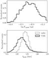 |
Fig. 10. Posterior distributions of the VHE peak flux density (top) and the radio (dashed grey line) and VHE (solid black line) peak times (bottom) for the “SSC (with KN)” fit of the afterglow of GW 170817. |
In the afterglow of GW 170817, the synchrotron spectrum is in the slow-cooling regime, with a spectral peak determined by the critical Lorentz factor γc. If IC scattering occurred in Thomson regime, the peak of the SSC component would be due to the scattering of photons at νc by the electrons at γc (Sari & Esin 2001), and this peak should be intense as ϵe ≫ ϵB (see Eq. (60)). However, the predicted VHE emission is very weak because the KN attenuation is strong. To illustrate this effect, we select in Table 6 two reference sets of parameters that are taken from the posterior sample. They are in the 68% and 97.5% confidence intervals for the “SSC (with KN)” fit and fit the observed light curves perfectly well. The first set of parameters (moderate) corresponds to a predicted VHE flux that is close to the median, whereas the second set of parameters (optimistic) corresponds to a predicted VHE flux at the highest end of the confidence interval (see the two predicted VHE light curves and peak spectra in Fig. 11). In both cases, we selected parameter sets with a low density and therefore, with a low energy (see the discussion in Sect. 4.3).
Parameters of the two reference cases.
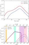 |
Fig. 11. VHE light curve at hνobs = 1 TeV (top) and spectrum around the peak at tobs = 110 days (bottom) for the moderate (in blue) and optimistic (in red) reference cases (see Table 6). Both predict similar fluxes in the synchrotron range due to the observational constraints, but they differ in the SSC regime. The upper limit from H.E.S.S. is indicated for comparison (Abdalla et al. 2020). |
Fig. 12 shows for these two reference cases the evolution of Y(γc) and  for the core jet. The SSC emission is either computed by assuming that all scatterings are in Thomson regime, as in the “SSC (Thomson)” fit, or by including the KN attenuation, as in the “SSC (with KN)” fit. The figure shows that in the full calculation,
  during the whole evolution, so that the scattering of photons at νc by electrons at γc is strongly reduced in the KN regime. The Compton parameter Y(γc) then remains very low. This confirms the origin of the weak VHE emission in the afterglow of GW 170817. In this regime of weak SSC emission, the synchrotron component is not affected by the IC cooling, γc ≃ γcsyn, and this explains why the results of the “no SSC” and “SSC (with KN)” fits are so close (Table 4). On the other hand, Fig. 12 also shows that Yno KN overestimates Y(γc) in this case, leading to Y(γc) > 1. The critical Lorentz factor is therefore given by γc ≃ γcsyn/Y(γc), which leads to an overestimation of γcsyn in the MCMC to maintain the cooling break above the X-ray measurements (increased E0,iso and lower ϵB). This explains the observed difference between the values of the model parameters inferred in the “SSC (Thomson)” and “SSC (with KN)” fits in Table 4. The value of
  in this case (green curves in the top panel of Fig. 12) proves that the Thomson regime is not justified.
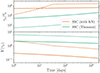 |
Fig. 12. Evolution of |

As the upper limit of H.E.S.S. was obtained close to the predicted peak with an already long exposure time of 53.9 hours (Abdalla et al. 2020), our prediction shows that it was unfortunately impossible to detect the VHE afterglow of GW 170817 with currently available instruments. We discuss the conditions that would make a post-merger afterglow detectable at VHE in the future in the next section, especially in the context of the increased sensitivity expected with the CTA.
5. Detectability of post-merger afterglows at very high energy, and prospects for the CTA
Even if the VHE afterglow of GW 170817 was not detectable, deeper observations of similar events can be expected in the future, in particular, with the CTA. The off-axis afterglow phase is of particular interest because after a few days, full-night observations can be conducted without a significant intrinsic source flux variability over the observation time. We investigate in this section the conditions that would make such an event detectable by current instruments and the upcoming CTA. For this study, we assumed a CTA detection sensitivity at 1 TeV about six times better than that of H.E.S.S., as expected from CTA Consortium et al. (2019). For an exposure time of ∼50 hours as for the H.E.S.S. deep observations of GW 170817 (Abdalla et al. 2020), this leads to a detection sensitivity at 1 TeV of 5 × 10⁻¹⁴ erg ⋅ s−1 ⋅ cm−2.
A geometrical effect such as a lower viewing angle naturally increases the peak of the observed flux, and it has a similar effect on the synchrotron and SSC components. In Fig. 13, we show the light curves (top) and spectra at the time of the 1 TeV emission peak (bottom) for the moderate reference case, and for gradually decreasing viewing angles. The 1 TeV light curves peak at earlier times when the viewing angle decreases, and the peak flux reaches higher values. As expected, the relative flux increase at the time of peak is similar for the synchrotron and the SSC components (Fig. 13, bottom), and all light curves follow a similar long-term evolution when the entire jet emission becomes visible to the off-axis observer. For the moderate (optimistic) reference case (Table 6), we find that a ratio θv/θc ≲ 3 (θv/θc ≲ 6) would have made the afterglow of GW 170817 detectable by H.E.S.S., provided the conditions had allowed for a very early deep observation. With the CTA, the VHE emission could have been detected up to θv/θc ≃ 4 (θv/θc ≃ 8). In this scenario, the emission peaks at ∼5 days (13 days). This opens up interesting perspectives even when the expected detection rate of nearby events at small viewing angles is low (see e.g. Duque et al. 2019; Mochkovitch et al. 2021).
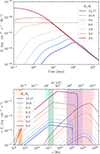 |
Fig. 13. Light curves at 1 TeV (top panel) and spectra at light-curve peak (bottom panel) of the moderate reference case (see Table 6) for varying viewing angles. The case fitting the afterglow of GW 170817 corresponds to θv/θc = 12.17. The peak times at which spectra are calculated are (in the ordering of the legend) 123, 73, 39, 17, 4.7, 1.4, and 0.06 days. The dotted line in the top panel corresponds to the assumed CTA sensitivity in Sect. 5. |
Under some conditions, the predicted VHE emission could also be intrinsically brighter. As discussed in Sect. 4.4, the VHE afterglow of GW 170817 is weak because of the strong KN attenuation ( ). The regime for the scattering of photons at νc by electrons at γc is affected by several parameters (Nakar 2007). When the scattering occurs in the Thomson regime, the predicted scaling in the core jet is
Therefore, the Thomson regime is favoured by a high magnetic field, a high density, or a high kinetic energy. As ϵB is determined by plasma instabilities at the ultra-relativistic shock (Sironi et al. 2015), it should not vary much from an afterglow to the next. On the other hand, the external density and the kinetic energy may differ between mergers. We focus here on the effect of the external density, which is slightly stronger. Fig. 14 shows the evolution of the afterglow emission for the moderate reference case when next increases up to ∼10 cm−3, all other parameters being kept constant. A higher external density leads to an earlier peak time at higher luminosities, but affects the synchrotron and the SSC flux differently: As expected, the SSC process becomes more efficient and the relative SSC-to-synchrotron ratio increases. The transition from the weak SSC emission due to a strong KN attenuation described in Sect. 4.4 to a more efficient case in Thomson regime occurs in this reference case above next ∼ 1 cm−3. This corresponds to the radiative regime S15 in Appendix B, with spectral breaks at  . This effect can clearly be observed in the bottom panel of Fig. 14, showing the observed spectrum at the peak emission. At the highest external densities, the increase in the VHE flux stalls for two reasons. Firstly, the strong SSC emission starts to affect the synchrotron spectrum significantly, which features two peaks (visible on the bottom panel of Fig. 14). The cooling frequency νc at the peak also decreases, shifting the SSC peak to lower frequencies so that the flux at 1 TeV does not increase as significantly as the SSC peak flux. A second limitation, dominant at the highest densities, comes from the pair production.
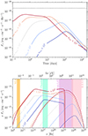 |
Fig. 14. Light curves at 1 TeV (top panel) and spectra at light-curve peak (bottom panel) of the moderate reference case (see Table 6) for varying external medium densities next. The case fitting the afterglow of GW 170817 corresponds to next = 4.25 × 10⁻³ cm−3. Each line is labelled with the multiplication factor applied to the reference next. The peak times at which spectra are calculated are 123, 60, 26, 12, and 0.55 days. The dotted line in the top panel corresponds to the assumed CTA sensitivity in Sect. 5. |
Even when these limitations are taken into account, a higher external density clearly favours a brighter VHE emission, even when both the moderate and optimistic reference cases remain undetectable by H.E.S.S. or the CTA at the reference viewing angle. We conclude that post-merger VHE afterglows should become detectable in the future only under several favourable conditions, such as a higher external density and a slightly lower viewing angle. For instance, the moderate (optimistic) reference case with an external density next = 1 cm−3 and a viewing angle θv/θc = 6 should be detectable by the CTA5 up to a distance of ∼90 Mpc (∼400 Mpc). However, two additional effects should be included in the optimistic case and may reduce this maximum distance: (i) At 400 Mpc, the attenuation by the extragalactic background light is no longer negligible at 1 TeV (see e.g. Domínguez et al. 2011), and (ii) in this case, the VHE afterglow peaks very early (∼1 day). This would require an early follow-up, which will necessarily be less deep due to a limited exposure time. Detections with the CTA above 100 Mpc remain possible in the optimistic case. As some parameters that are naturally degenerate in an afterglow fit including only synchrotron radiation, such as next and ϵB, have different effects on the SSC emission, these VHE detections would therefore better constrain the parameter space and allow for a better understanding of the physical conditions in the post-merger relativistic ejecta.
Another direct consequence of the impact of next on SSC emission is that short GRB afterglows detected at VHE are more likely to originate from mergers that occur in a denser environment. These VHE detections could therefore be unique probes of high-density media at the location of BNS mergers, which are sought clues for binaries with short merger times. Fast mergers are indeed expected to occur close to their formation sites, where the external medium density is expected to be higher (see e.g. the discussion in Duque et al. 2020). Population synthesis studies have shown that the as yet poorly constrained common-envelope phase during the binary star evolution can lead to the production of BNS with very short initial separations that merge rapidly, as discussed for instance by Dominik et al. (2012). Favourable kick intensities and orientations during the supernovae could also tend to shrink the initial orbital separation and increase the orbital eccentricity for part of the BNS population (Kalogera 1996). Observationally, the projected offset distribution of BNS mergers in their host galaxy seems to feature a tail below one half-light radius for ∼20% of the systems (Fong & Berger 2013; Berger 2014). These observations have several observational biases, such as afterglow detection, host galaxy association, and projection effects, which probably leads to sample incompleteness, but they give evidence for a population of fast mergers. If BNS mergers are the dominant site for r-process nucleosynthesis (see e.g. Lattimer & Schramm 1974; Goriely et al. 2011; Just et al. 2015; Côté et al. 2017), another more indirect evidence is provided by the observed large scatter of [Eu/Fe] abundances in extremely metal-poor stars (see the compilation by Suda et al. 2008), which requires fast mergers that allow the production of r-process elements when the environment is still extremely metal poor (see e.g. Vangioni et al. 2016; Côté et al. 2019; Dvorkin et al. 2021). It has already been suggested by Duque et al. (2020) that multi-messenger observations of BNS, including the detection of the afterglow, will be biased in favour of a high-density environment, thus allowing us to probe this potential population of fast mergers. We showed here that future VHE afterglow detections either following the GW detection of a BNS merger or the detection of a short GRB can also probe this population directly.
6. Conclusion
We developed a detailed model of the afterglow of a laterally structured jet from radio to VHE. Emission is produced in the shocked external medium behind the forward external shock, and the dynamics does not include the late lateral expansion of the ejecta. These effects, as well as the contribution of the reverse shock, will be implemented in the future. The main challenge addressed in this paper is the self-consistent calculation of the synchrotron and SSC emission while accounting for the two different IC regimes, the Thomson and KN regime. We based our approach on the method proposed by Nakar et al. (2009), which we extended to include additional effects: The maximum electron Lorentz factor γmax was also computed self-consistently, leading to a realistic estimate of the high-energy cutoff of the synchrotron component, and the attenuation at high-energy due to pair production was included as well. The values of γc and Y(γc) and of the spectral regimes were determined numerically. Synchrotron self-absorption, which is relevant at low radio frequencies, is not yet included. The implementation of the model is computationally efficient and allows a fitting of afterglow data.
We used this model to fit the multi-wavelength afterglow of GW 170817, including radio to X-ray observations up to 400 days and five early-time upper limits. We inferred the model parameters using three different assumptions for the emission: (i) Purely synchrotron, (ii) synchrotron and SSC, assuming that scatterings occur in Thomson regime, and (iii) self-consistent synchrotron and SSC calculation taking the KN regime into account. We obtained excellent fits in the three cases, with similar constraints on the parameters for the purely synchrotron case and the full calculation with SSC in KN regimes, whereas the case in which scattering was assumed to be in the Thomson regime deviated significantly. The SSC emission in the afterglow of GW 170817 is indeed weak due to the strong KN attenuation, which confirms the need to include the self-consistent calculation of the SSC emission in the KN regime in afterglow models. The predicted VHE flux at the peak has a large dispersion, but remains about two orders of magnitude below the upper limit obtained around the peak by H.E.S.S. This shows that the VHE afterglow of GW 170817 was undetectable by current instruments, but that future detections of similar events would break some degeneracies among the model parameters and would provide better constraints on the physics of the relativistic ejecta.
We then studied how these post-merger VHE afterglows may become detectable in the future in the context of the improved sensitivity of the CTA. Beyond the evident effect of a less off-axis viewing angle, we showed that the efficiency of the SSC emission becomes higher in external media with higher densities than GW 170817. For instance, a similar ultra-relativistic jet in a medium with a density of ∼1 cm−3 and seen slightly less off-axis than GW 170817 may become detectable by the CTA at 100–400 Mpc.
This bias of VHE afterglow detections in favour of high-density environments offers a new probe of a possible population of fast mergers. With a short merger time, a merger should indeed occur in more central, and denser, regions of its host galaxy. Thus, future detections of these VHE afterglows would not only advance our physical understanding of relativistic jets that are produced after a BNS merger, but would also constrain the physics of the evolution of massive binary systems.
Candidate VHE photons are associated at a lower level of confidence with several other bursts by MAGIC, including the short GRB 160821B (Acciari et al. 2021).
Data points are provided by K. Mooley on https://github.com/kmooley/GW170817/
The emission in the 0.1 − 1 GeV range is then dominated by the synchrotron radiation. For comparison with Fig. 9, the sensitivity of Fermi/LAT above 100 MeV is of the order of 10−11 erg ⋅ s−1 ⋅ cm−2 for a ∼1 day observation (Abdollahi et al. 2020, 2022). The afterglow of GW 170817 was therefore undetectable by Fermi/LAT at any time.
Acknowledgments
Clément Pellouin acknowledges funding support from the Initiative Physique des Infinis (IPI), a research training program of the Idex SUPER at Sorbonne University. The authors acknowledge the Centre National d’Études Spatiales (CNES) for financial support in this research project. This work made use of the Infinity computing cluster at IAP. The authors thank K. Mooley for providing GW 170817 afterglow observation data at https://github.com/kmooley/GW170817/. This work made use of Python 3.8 and of the Python packages arviz (Kumar et al. 2019), astropy (Astropy Collaboration 2022), corner (Foreman-Mackey 2016), emcee (Foreman-Mackey et al. 2019, 2013), matplotlib (Hunter 2007), multiprocessing, numpy (Harris et al. 2020), pandas (McKinney 2010), scipy (Virtanen et al. 2020).
References
- Abbott, B. P., Abbott, R., Abbott, T. D., et al. 2017a, ApJ, 848, L12 [Google Scholar]
- Abbott, B. P., Abbott, R., Abbott, T. D., et al. 2017b, Phys. Rev. Lett., 119, 161101 [Google Scholar]
- Abdalla, H., Abramowski, A., Aharonian, F., et al. 2017, ApJ, 850, L22 [NASA ADS] [CrossRef] [Google Scholar]
- Abdalla, H., Adam, R., Aharonian, F., et al. 2019, Nature, 575, 464 [Google Scholar]
- Abdalla, H., Adam, R., Aharonian, F., et al. 2020, ApJ, 894, L16 [NASA ADS] [CrossRef] [Google Scholar]
- Abdollahi, S., Acero, F., Ackermann, M., et al. 2020, ApJS, 247, 33 [Google Scholar]
- Abdollahi, S., Acero, F., Baldini, L., et al. 2022, ApJS, 260, 53 [NASA ADS] [CrossRef] [Google Scholar]
- Acciari, V. A., Ansoldi, S., Antonelli, L. A., et al. 2021, ApJ, 908, 90 [NASA ADS] [CrossRef] [Google Scholar]
- Ajello, M., Allafort, A., Axelsson, M., et al. 2018, ApJ, 861, 85 [NASA ADS] [CrossRef] [Google Scholar]
- Aksulu, M. D., Wijers, R. A. M. J., van Eerten, H. J., & van der Horst, A. J. 2022, MNRAS, 511, 2848 [NASA ADS] [CrossRef] [Google Scholar]
- Ascenzi, S., Oganesyan, G., Salafia, O. S., et al. 2020, A&A, 641, A61 [NASA ADS] [CrossRef] [EDP Sciences] [Google Scholar]
- Astropy Collaboration (Price-Whelan, A. M., et al.) 2022, ApJ, 935, 167 [NASA ADS] [CrossRef] [Google Scholar]
- Balasubramanian, A., Corsi, A., Mooley, K. P., et al. 2021, ApJ, 914, L20 [NASA ADS] [CrossRef] [Google Scholar]
- Beniamini, P., Nava, L., Duran, R. B., & Piran, T. 2015, MNRAS, 454, 1073 [NASA ADS] [CrossRef] [Google Scholar]
- Beniamini, P., Duque, R., Daigne, F., & Mochkovitch, R. 2020a, MNRAS, 492, 2847 [NASA ADS] [CrossRef] [Google Scholar]
- Beniamini, P., Granot, J., & Gill, R. 2020b, MNRAS, 493, 3521 [NASA ADS] [CrossRef] [Google Scholar]
- Berger, E. 2014, ARA&A, 52, 43 [CrossRef] [Google Scholar]
- Blanch, O., Longo, F., Berti, A., et al. 2020, GRB Coordinates Network, 29075, 1 [NASA ADS] [Google Scholar]
- Blandford, R. D., & McKee, C. F. 1976, Phys. Fluids, 19, 1130 [Google Scholar]
- Bošnjak, Ž., Daigne, F., & Dubus, G. 2009, A&A, 498, 677 [NASA ADS] [CrossRef] [EDP Sciences] [Google Scholar]
- Bromberg, O., Nakar, E., Piran, T., & Sari, R. 2011, ApJ, 740, 100 [NASA ADS] [CrossRef] [Google Scholar]
- Bromberg, O., Tchekhovskoy, A., Gottlieb, O., Nakar, E., & Piran, T. 2018, MNRAS, 475, 2971 [NASA ADS] [CrossRef] [Google Scholar]
- Cantiello, M., Jensen, J. B., Blakeslee, J. P., et al. 2018, ApJ, 854, L31 [Google Scholar]
- Cherenkov Telescope Array Consortium, Acharya, B. S., Agudo, I., et al. 2019, Science with the Cherenkov Telescope Array (World Scientific) [Google Scholar]
- Côté, B., Belczynski, K., Fryer, C. L., et al. 2017, ApJ, 836, 230 [CrossRef] [Google Scholar]
- Côté, B., Eichler, M., Arcones, A., et al. 2019, ApJ, 875, 106 [Google Scholar]
- Cowperthwaite, P. S., Berger, E., Villar, V. A., et al. 2017, ApJ, 848, L17 [CrossRef] [Google Scholar]
- Daigne, F., & Mochkovitch, R. 1998, MNRAS, 296, 275 [NASA ADS] [CrossRef] [Google Scholar]
- Daigne, F., & Mochkovitch, R. 2000, A&A, 358, 1157 [NASA ADS] [Google Scholar]
- D’Avanzo, P., Campana, S., Salafia, O. S., et al. 2018, A&A, 613, L1 [NASA ADS] [CrossRef] [EDP Sciences] [Google Scholar]
- Derishev, E., & Piran, T. 2021, ApJ, 923, 135 [CrossRef] [Google Scholar]
- Derishev, E., & Piran, T. 2024, MNRAS, 530, 347 [NASA ADS] [CrossRef] [Google Scholar]
- Derishev, E. V., Kocharovsky, V. V., & Kocharovsky, V. V. 2001, A&A, 372, 1071 [NASA ADS] [CrossRef] [EDP Sciences] [Google Scholar]
- Domínguez, A., Primack, J. R., Rosario, D. J., et al. 2011, MNRAS, 410, 2556 [Google Scholar]
- Dominik, M., Belczynski, K., Fryer, C., et al. 2012, ApJ, 759, 52 [Google Scholar]
- Duffell, P. C., & Laskar, T. 2018, ApJ, 865, 94 [NASA ADS] [CrossRef] [Google Scholar]
- Duque, R., Daigne, F., & Mochkovitch, R. 2019, A&A, 631, A39 [NASA ADS] [CrossRef] [EDP Sciences] [Google Scholar]
- Duque, R., Beniamini, P., Daigne, F., & Mochkovitch, R. 2020, A&A, 639, A15 [NASA ADS] [CrossRef] [EDP Sciences] [Google Scholar]
- Duque, R., Beniamini, P., Daigne, F., & Mochkovitch, R. 2022, MNRAS, 513, 951 [CrossRef] [Google Scholar]
- Dvorkin, I., Daigne, F., Goriely, S., Vangioni, E., & Silk, J. 2021, MNRAS, 506, 4374 [NASA ADS] [CrossRef] [Google Scholar]
- Finstad, D., De, S., Brown, D. A., Berger, E., & Biwer, C. M. 2018, ApJ, 860, L2 [NASA ADS] [CrossRef] [Google Scholar]
- Fong, W., & Berger, E. 2013, ApJ, 776, 18 [NASA ADS] [CrossRef] [Google Scholar]
- Fong, W., Berger, E., Margutti, R., & Zauderer, B. A. 2015, ApJ, 815, 102 [NASA ADS] [CrossRef] [Google Scholar]
- Foreman-Mackey, D. 2016, J. Open Source Software, 1, 24 [NASA ADS] [CrossRef] [Google Scholar]
- Foreman-Mackey, D., Hogg, D. W., Lang, D., & Goodman, J. 2013, PASP, 125, 306 [Google Scholar]
- Foreman-Mackey, D., Farr, W., Sinha, M., et al. 2019, J. Open Source Software, 4, 1864 [CrossRef] [Google Scholar]
- Galván, A., Fraija, N., & González, M. M. 2019, Int. Cosmic Ray Conf., 36, 681 [CrossRef] [Google Scholar]
- Genet, F., Daigne, F., & Mochkovitch, R. 2007, MNRAS, 381, 732 [NASA ADS] [CrossRef] [Google Scholar]
- Ghirlanda, G., Salafia, O. S., Paragi, Z., et al. 2019, Science, 363, 968 [NASA ADS] [CrossRef] [Google Scholar]
- Gill, R., & Granot, J. 2018, MNRAS, 478, 4128 [NASA ADS] [CrossRef] [Google Scholar]
- Gill, R., & Granot, J. 2022, Galaxies, 10, 74 [CrossRef] [Google Scholar]
- Gill, R., & Granot, J. 2023, MNRAS, 524, L78 [NASA ADS] [CrossRef] [Google Scholar]
- Goldstein, A., Veres, P., Burns, E., et al. 2017, ApJ, 848, L14 [CrossRef] [Google Scholar]
- Goriely, S., Bauswein, A., & Janka, H.-T. 2011, ApJ, 738, L32 [Google Scholar]
- Gottlieb, O., Nakar, E., Piran, T., & Hotokezaka, K. 2018, MNRAS, 479, 588 [NASA ADS] [Google Scholar]
- Govreen-Segal, T., & Nakar, E. 2023, MNRAS, 524, 403 [NASA ADS] [CrossRef] [Google Scholar]
- Granot, J., & Piran, T. 2012, MNRAS, 421, 570 [Google Scholar]
- Granot, J., Piran, T., & Sari, R. 1999, ApJ, 513, 679 [NASA ADS] [CrossRef] [Google Scholar]
- H.E.S.S. Collaboration (Abdalla, H., et al.) 2021, Science, 372, 1081 [NASA ADS] [CrossRef] [Google Scholar]
- Hajela, A., Margutti, R., Alexander, K. D., et al. 2019, ApJ, 886, L17 [NASA ADS] [CrossRef] [Google Scholar]
- Hajela, A., Margutti, R., Bright, J. S., et al. 2022, ApJ, 927, L17 [NASA ADS] [CrossRef] [Google Scholar]
- Hallinan, G., Corsi, A., Mooley, K. P., et al. 2017, Science, 358, 1579 [NASA ADS] [CrossRef] [Google Scholar]
- Harris, C. R., Millman, K. J., van der Walt, S. J., et al. 2020, Nature, 585, 357 [NASA ADS] [CrossRef] [Google Scholar]
- Hunter, J. D. 2007, Comput. Sci. Eng., 9, 90 [NASA ADS] [CrossRef] [Google Scholar]
- Jacovich, T. E., Beniamini, P., & van der Horst, A. J. 2021, MNRAS, 504, 528 [CrossRef] [Google Scholar]
- Just, O., Bauswein, A., Ardevol Pulpillo, R., Goriely, S., & Janka, H. T. 2015, MNRAS, 448, 541 [NASA ADS] [CrossRef] [Google Scholar]
- Kalogera, V. 1996, ApJ, 471, 352 [Google Scholar]
- Kann, D. A., Agayeva, S., Aivazyan, V., et al. 2023, ApJ, 948, L12 [NASA ADS] [CrossRef] [Google Scholar]
- Kobayashi, S., Piran, T., & Sari, R. 1997, ApJ, 490, 92 [Google Scholar]
- Kumar, R., Carroll, C., Hartikainen, A., & Martin, O. 2019, J. Open Source Software, 4, 1143 [NASA ADS] [CrossRef] [Google Scholar]
- Lamb, G. P., Lyman, J. D., Levan, A. J., et al. 2019, ApJ, 870, L15 [NASA ADS] [CrossRef] [Google Scholar]
- Laskar, T., Alexander, K. D., Margutti, R., et al. 2023, ApJ, 946, L23 [NASA ADS] [CrossRef] [Google Scholar]
- Lattimer, J. M., & Schramm, D. N. 1974, ApJ, 192, L145 [NASA ADS] [CrossRef] [Google Scholar]
- LHAASO Collaboration 2023, Science, 380, 1390 [NASA ADS] [CrossRef] [Google Scholar]
- MAGIC Collaboration (Acciari, V. A., et al.) 2019a, Nature, 575, 455 [Google Scholar]
- MAGIC Collaboration (Acciari, V. A., et al.) 2019b, Nature, 575, 459 [Google Scholar]
- Makhathini, S., Mooley, K. P., Brightman, M., et al. 2021, ApJ, 922, 154 [NASA ADS] [CrossRef] [Google Scholar]
- Matsumoto, T., Nakar, E., & Piran, T. 2019, MNRAS, 483, 1247 [NASA ADS] [CrossRef] [Google Scholar]
- McKinney, W. 2010, in Proceedings of the 9th Python in Science Conference, eds. S. van der Walt, & J. Millman, 56 [Google Scholar]
- Mochkovitch, R., Daigne, F., Duque, R., & Zitouni, H. 2021, A&A, 651, A83 [NASA ADS] [CrossRef] [EDP Sciences] [Google Scholar]
- Mooley, K. P., Deller, A. T., Gottlieb, O., et al. 2018, Nature, 561, 355 [Google Scholar]
- Mooley, K. P., Anderson, J., & Lu, W. 2022, Nature, 610, 273 [NASA ADS] [CrossRef] [Google Scholar]
- Murase, K., Toma, K., Yamazaki, R., & Mészáros, P. 2011, ApJ, 732, 77 [NASA ADS] [CrossRef] [Google Scholar]
- Nakar, E. 2007, Phys. Rep., 442, 166 [NASA ADS] [CrossRef] [Google Scholar]
- Nakar, E., & Piran, T. 2011, Nature, 478, 82 [NASA ADS] [CrossRef] [Google Scholar]
- Nakar, E., & Piran, T. 2018, MNRAS, 478, 407 [NASA ADS] [CrossRef] [Google Scholar]
- Nakar, E., & Piran, T. 2021, ApJ, 909, 114 [NASA ADS] [CrossRef] [Google Scholar]
- Nakar, E., Ando, S., & Sari, R. 2009, ApJ, 703, 675 [NASA ADS] [CrossRef] [Google Scholar]
- O’Connor, B., Troja, E., Ryan, G., et al. 2023, Sci. Adv., 9, eadi1405 [CrossRef] [Google Scholar]
- Oganesyan, G., Ascenzi, S., Branchesi, M., et al. 2020, ApJ, 893, 88 [NASA ADS] [CrossRef] [Google Scholar]
- Palmese, A., Hartley, W., Tarsitano, F., et al. 2017, ApJ, 849, L34 [NASA ADS] [CrossRef] [Google Scholar]
- Panaitescu, A., & Kumar, P. 2000, ApJ, 543, 66 [Google Scholar]
- Piran, T., & Nakar, E. 2010, ApJ, 718, L63 [NASA ADS] [CrossRef] [Google Scholar]
- Rhoads, J. E. 1997, ApJ, 487, L1 [NASA ADS] [CrossRef] [Google Scholar]
- Ryan, G., van Eerten, H., Piro, L., & Troja, E. 2020, ApJ, 896, 166 [CrossRef] [Google Scholar]
- Salafia, O. S., Berti, A., Covino, S., et al. 2022a, in 37th International Cosmic Ray Conference, 944 [Google Scholar]
- Salafia, O. S., Ravasio, M. E., Yang, J., et al. 2022b, ApJ, 931, L19 [NASA ADS] [CrossRef] [Google Scholar]
- Sari, R., & Esin, A. A. 2001, ApJ, 548, 787 [NASA ADS] [CrossRef] [Google Scholar]
- Sari, R., Piran, T., & Narayan, R. 1998, ApJ, 497, L17 [Google Scholar]
- Sato, Y., Murase, K., Ohira, Y., & Yamazaki, R. 2023, MNRAS, 522, L56 [NASA ADS] [CrossRef] [Google Scholar]
- Savchenko, V., Ferrigno, C., Kuulkers, E., et al. 2017, ApJ, 848, L15 [NASA ADS] [CrossRef] [Google Scholar]
- Sedov, L. I. 1946, J. Appl. Math. Mech., 10, 241 [Google Scholar]
- Sironi, L., Keshet, U., & Lemoine, M. 2015, Space. Sci. Rev., 191, 519 [NASA ADS] [CrossRef] [Google Scholar]
- Suda, T., Katsuta, Y., Yamada, S., et al. 2008, PASJ, 60, 1159 [NASA ADS] [Google Scholar]
- Tanvir, N. R., Levan, A. J., González-Fernández, C., et al. 2017, ApJ, 848, L27 [CrossRef] [Google Scholar]
- Taylor, G. 1950, Proc. R. Soc. London Ser. A, 201, 159 [Google Scholar]
- Troja, E., van Eerten, H., Ryan, G., et al. 2019, MNRAS, 489, 1919 [NASA ADS] [Google Scholar]
- Troja, E., van Eerten, H., Zhang, B., et al. 2020, MNRAS, 498, 5643 [NASA ADS] [CrossRef] [Google Scholar]
- Troja, E., O’Connor, B., Ryan, G., et al. 2022, MNRAS, 510, 1902 [Google Scholar]
- Uhm, Z. L., & Beloborodov, A. M. 2007, ApJ, 665, L93 [NASA ADS] [CrossRef] [Google Scholar]
- van Eerten, H. J., & MacFadyen, A. I. 2012, ApJ, 747, L30 [NASA ADS] [CrossRef] [Google Scholar]
- van Eerten, H., van der Horst, A., & MacFadyen, A. 2012, ApJ, 749, 44 [NASA ADS] [CrossRef] [Google Scholar]
- Vangioni, E., Goriely, S., Daigne, F., François, P., & Belczynski, K. 2016, MNRAS, 455, 17 [NASA ADS] [CrossRef] [Google Scholar]
- Villar, V. A., Guillochon, J., Berger, E., et al. 2017, ApJ, 851, L21 [Google Scholar]
- Virtanen, P., Gommers, R., Oliphant, T. E., et al. 2020, Nat. Meth., 17, 261 [Google Scholar]
- Wang, X.-Y., Liu, R.-Y., Zhang, H.-M., Xi, S.-Q., & Zhang, B. 2019, ApJ, 884, 117 [NASA ADS] [CrossRef] [Google Scholar]
- Wang, H., Dastidar, R. G., Giannios, D., & Duffell, P. C. 2024, ApJS, submitted [arXiv:2402.19359] [Google Scholar]
- Warren, D. C., Dainotti, M., Barkov, M. V., et al. 2022, ApJ, 924, 40 [NASA ADS] [CrossRef] [Google Scholar]
- Woods, E., & Loeb, A. 1999, ApJ, 523, 187 [NASA ADS] [CrossRef] [Google Scholar]
- Yamasaki, S., & Piran, T. 2022, MNRAS, 512, 2142 [NASA ADS] [CrossRef] [Google Scholar]
- Zhang, B., Wang, X.-Y., & Zheng, J.-H. 2024, J. High Energy Astrophys., 41, 42 [NASA ADS] [CrossRef] [Google Scholar]
- Zheng, J.-H., Wang, X.-Y., Liu, R.-Y., & Zhang, B. 2024, ApJ, 966, 141 [NASA ADS] [CrossRef] [Google Scholar]
Appendix A: Maximum electron Lorentz factor and synchrotron burnoff limit
The maximum Lorentz factor γmax of accelerated electrons is defined in Sect. 2.3 and is reached when the acceleration timescale becomes longer than the cooling timescale,

where the dynamical timescale tdyn and the acceleration timescale tacc are defined by Eqs. (16) and (24). From Eqs. (38) and (39), the radiative timescale trad is given by
Eq. (A.1) can then be rewritten
![$$ \begin{aligned} \mathrm{min} \left[ 1; \frac{\gamma _{\rm c}^\mathrm{syn}}{\gamma _{\rm max} (1+Y(\gamma _{\rm max}))} \right] = \widetilde{K} \gamma _{\rm max}\, , \end{aligned} $$](/articles/aa/full_html/2024/10/aa47516-23/aa47516-23-eq197.gif)
with
Then γmax is the solution of
![$$ \begin{aligned} \gamma _{\rm max}^2 [1+Y(\gamma _{\rm max})] = \frac{\gamma _{\rm c}^\mathrm{syn}}{\widetilde{K}} \end{aligned} $$](/articles/aa/full_html/2024/10/aa47516-23/aa47516-23-eq199.gif)
except in unlikely cases where electrons at γmax are slow cooling (γmax < γc), that lead to  .
.
In the current version of the model, we assume γmax ≫ γm so that the calculation of γc and the identification of the radiative regime and associated normalised electron distribution f(x) and Compton parameter h(x) are independent of γmax (see Sect. 2.4.6). Therefore the maximum Lorentz factor is determined once this radiative regime is identified. We follow an iterative procedure where the segments of h(x) are explored successively starting from the last segment  (highest Lorentz factors):
-
We check if there is a solution of Eq. (A.5) in this segment, with the usual approximation for 1 + Y,
where Y(γmax) is computed from Eq. (62), which leads to
The pre-factor A is the same as in Eq. (66).
-
If there is a solution in the considered segment, we stop the iterative procedure and keep the following value for the maximum electron Lorentz factor:
-
the solution γmax found in the segment if γmax > γc (fast cooling);
-
the solution
 otherwise (slow cooling).
-
-
If there is no solution in the considered segment:
-
If the next segment is still at least partially in fast-cooling regime (i.e. the upper bound is above γc), we start a new iteration at step 1. using this new segment;
-
otherwise we stop the iterative procedure and keep for γmax the slow-cooling solution
 .
.
-
In most cases, the maximum electron Lorentz factor is large enough to be in fast-cooling regime (γmax > γc so that trad(γmax) < tdyn) with a negligible IC cooling (Y(γmax) < 1). In this case, the maximum Lorentz factor  leads to the usual synchrotron burnoff limit (see e.g. Piran & Nakar 2010) for the high-frequency cutoff of the synchrotron spectrum in the comoving frame
  :
:
For the best-fit parameters of the afterglow of GW 170817 presented in Sect. 4, the Lorentz factor of the core jet at tpeak is Γ ≃ 10. The limit is thus expected at ∼1 GeV in the observer frame, as seen in Fig. 9.
Appendix B: Radiative regimes and corresponding electron distributions
 |
Fig. B.1. Definition of all possible cases for the radiative regime and the distribution of electrons in the plane γ0 vs γself. The Lorentz factors γm and γc are indicated by red and green solid lines either in the fast-cooling regime with γm > γc (left) or in the slow-cooling regime with γm < γc (right). The black solid line in the left panel corresponds to γ0 = γself. The two Lorentz factors |


The IC cooling impacts the distribution of electrons if  (Eq. (65)). As

all possibles cases regarding the radiative regime and the distribution of electrons can be identified in the (γself;γ0) plane shown in Fig. B.1. As an electron of Lorentz factor γ can upscatter its own synchrotron photon only if  , that is, if γ ≤ γself, the x-axis quantifies the importance of the KN suppression: the lower γself (left side of the diagram), the more electrons are affected by KN effects. The y-axis quantifies the importance of IC cooling: the IC power of all electrons with γ > γ0 is negligible compared to the synchrotron power. Therefore, the lower γ0 (bottom of the diagram), the more electrons have a negligible IC cooling. We list in Tables B.1 (fast cooling) and B.2 (slow cooling) all these cases and provide the corresponding self-consistent solution (breaks and slopes) for the normalised distribution of electrons f(x) (Eq. (43)) and the normalised Compton parameter h(x) (Eq. (62)), as obtained following the detailed method described in Nakar et al. (2009). The break corresponding to the peak of the synchrotron spectrum is highlighted in red. We also provide in each case the expression of γ0 obtained from the relation Y(γc) = h(xc)/h(x0) (Eq. (67)), as needed in the iterative procedure to determine Y(γc): see Sect. 2.4.6.
The distribution of electrons is unaffected by the SSC cooling when γ0 < γc or  . These two regions are shaded in orange and blue in Fig. B.1. When
  (cases F1 and S1), the IC cooling is negligible for all electrons and γ0 is undefined. The solution is provided by the purely synchrotron case (Sect. 2.4.4). When
  (cases F2 to F5 and S2 to S6), the normalised electron distribution f(x) is also the same as in the purely synchrotron case but γ0 is defined and its expression depends on the considered regime.
In all other cases, the SSC cooling affects the distribution of electrons and the synchrotron spectrum, with additional breaks (N ≥ 3), as listed in Tables B.1 and B.2. There are more subcases in fast cooling. The most relevant ones for GRB afterglows are discussed in Nakar et al. (2009): their case I with its two subcases correspond to F26 and F27; their case IIa to F20-F21, their case IIb to F22-F23; their cases IIc and III to some subcases of F24 and F25.
Cases F24 and F25 are indeed more complex and require a specific treatment (see Sect. 3.2 Nakar et al. 2009), as a large number of breaks can appear in the distribution, that must be found iteratively. These two cases correspond to  . New breaks will appear in the spectral shape f(x) every time that
  , where using Eq. (B.1), we define the successive
  as
as
This condition is equivalent to γself = γself, cr, 2n, where
with n ≥ 1. For n = 1, the first value  is plotted in Fig. B.1 and is the frontier at low γself of the cases F24 and F25. On the other hand γself, cr, 2n tends to γm when n tends to infinity, that is, the frontier at high γself. Then, the values of γself, cr, 2n for n > 1 divide F24 and F25 in many sub-regions. We define the column n by the condition γself, cr, 2n < γself < γself, cr, 2n + 2. In practice, γself, cr, 2n rapidly converges, and the spectral shapes in these narrower columns rapidly become closer and closer to each other. This allows numerically to not distinguish columns above a certain nmax. We use nmax = 7.
In each column n, cases F24 and F25 are then divided in several subcases depending on the relative position of γ0 and  ,
,  and
and  with k ≥ 1. In each subcase, the list of breaks and slopes can be determined for f(x) and h(x), as well as the position of the peak of the synchrotron spectrum. We show for illustration the results in the two first columns in Table B.3.
Fast cooling: list of all possible radiative regimes and corresponding electron distribution.
Slow cooling: list of all possible radiative regimes and corresponding electron distribution.
Fast cooling cases F24 and F25.
Appendix C: Posterior distributions of the three fits of the afterglow of GW 170817
Fig. C.1 gives the posterior joint and marginalised distributions of the model parameters for the three fits of the multi-wavelength afterglow of GW 170817 described in Sect. 4. The three fits use the same observational constraints and the same priors on the free parameters, and differ only by the radiative treatment: synchrotron only ("no SSC"), synchrotron and SSC assuming that all IC scatterings occur in Thomson regime ("SSC (Thomson)"), and self-consistent calculation of synchrotron and SSC processes taking into account the KN attenuation ("SSC (with KN)"). It appears clearly that the "no SSC" and "SSC (with KN)" fits lead to similar results, whereas the parameters inferred by the "SSC (Thomson)" fit are slighltly different (see also Table 4). This especially true for the viewing and core jet opening angles, but also for the kinetic energy and the external density. Note the correlations between these quantities. This difference is due to the fact that the SSC component in the afterglow of GW 170817 is very weak due to the KN attenuation, and is therefore overestimated in the "SSC (Thomson)" case: see discussion in Sect. 4.3.
 |
Fig. C.1. Posterior joint and marginalised distributions of the free model parameters, E0, isoc, θc, θv, next, ϵB, ϵe, ζ, pa, Γ0c, b for the three fits of the afterglow of GW 170817 presented in Sect. 4, which differ only by the treatment of the radiative processes. In blue, no SSC scatterings are taken into account ("no SSC"); in green, SSC scatterings are assumed to be only in the Thomson regime ("SSC (Thomson)"); in orange, the SSC scattering is depleted at high energy in the KN regime ("SSC (with KN)"). The coloured contours correspond to the 3σ confidence intervals for each model and each parameter. |
All Tables
Values of the dimensionless parameters KP; Kν and KPmax for different afterglow models used in each reference.
Posterior values for the free parameters of the three fits of the afterglow of GW 170817.
Posterior values for several derived quantities from the three fits of the afterglow of GW 170817.
Fast cooling: list of all possible radiative regimes and corresponding electron distribution.
Slow cooling: list of all possible radiative regimes and corresponding electron distribution.
All Figures
|
Fig. 1. Coordinates and notations used in the expression of the observed flux. |
| In the text | |
|
Fig. 2. Synthetic afterglow light curves of a top-hat jet viewed on-axis in the synchrotron-only radiation regime. The solid lines show the results obtained using our model with full dynamics treatment (using Eq. (10)). The dotted lines follow the self-similar solution at all times. The dashed lines are obtained with afterglowpy without lateral expansion. The fluxes are computed in radio at 3 GHz (black), in optical in r band at 5.06 × 10¹⁴ Hz (blue), and in X-rays at 1 keV (red). The parameters used for this figure are E0, iso = 1052 erg, θc = 4 deg, next = 10−3 cm−3, ϵe = 10−1, ϵB = 10−1, p = 2.2, and DL = 100 Mpc. |
| In the text | |
|
Fig. 3. Spectral fits to the afterglow observations of GRB 190114C at 90 s (black data points taken from MAGIC Collaboration 2019b). Each colour represents the best-fit spectrum for each of the possible radiative regimes (see text and Fig. 4). The spectral cases are detailed in Appendix B. This figure can be compared to Fig. 6 in Yamasaki & Piran (2022), which shows very similar fits. |
| In the text | |
|
Fig. 4. Marginalised posterior distributions for the spectral fit of the afterglow observations of GRB 190114C at tobs = 90 s. The total (black) is subdivided between the slow (blue) and fast (red) cooling cases. The first row shows the four free parameters explored in this MCMC analysis (Γ, ϵe/ϵB, B and γm). In the second row, we show some derived quantities: |
| In the text | |
|
Fig. 5. Comparison of the marginalised posterior distributions for the three fits of the afterglow of GW 170817 presented in Sect. 4, which differ only by the treatment of the radiative processes: “no SSC” in blue; “SSC (Thomson)” in green; “SSC (with KN)” in orange. The first two rows show the inferred distributions of the free model parameters. The last row shows the distributions of several quantities derived from these parameters: The true energy of the jet E0 (see Eq. (5)), the ratio θv/θc, and the four quantities used in the conditions for single-peaked light curves from Beniamini et al. (2020b) and described in Sect. 2.2, log(θcΓ0c), 8b/a, |
| In the text | |
|
Fig. 6. Posterior joint and marginalised distributions of the free model parameters, E0, isoc, θc, θv, next, ϵB, ϵe, ζ, pa, Γ0c, b, for the “SSC (with KN)” fit of the afterglow of GW 170817 presented in Sect. 4, which includes SSC scatterings in the Thomson and KN regimes. The priors are all uniform or log-uniform and are shown in Table 3. The fitted data include all points until tmax = 400 days, as well as five early-time upper limits (see Sect. 4.1). The coloured contours correspond to the 1σ, 2σ, and 3σ confidence intervals for each parameter. |
| In the text | |
|
Fig. 7. Posterior distribution of the radio light curves at νobs = 3 GHz for the “SSC (with KN)” fit of the afterglow of GW 170817. The solid lines represent the median value at each observing time, the dark contours are the 68% confidence interval, and the light contours show the 97.5% confidence interval. Late-time observations that were not used in the fit are shown in blue. |
| In the text | |
|
Fig. 8. Posterior distribution of the VHE light curves at hνobs = 1 TeV for the “SSC (with KN)” fit of the afterglow of GW 170817. Same as in Fig. 7. This is a prediction of the model. No observational constraint is included in the fit. |
| In the text | |
|
Fig. 9. Posterior distribution of the afterglow spectrum around its peak (tobs = 110 days) for the “SSC (with KN)” fit of the afterglow of GW 170817. The data points show the multi-wavelength observations at tobs ± 4 days. The upper limit from H.E.S.S. is also indicated (Abdalla et al. 2020). The low-energy component (solid line) is produced by synchrotron radiation, while the high-energy emission (dashed line) is powered by SSC scattering. The thick lines represent the median value at each observing frequency, the dark contours show the 68% confidence interval, and the light contours present the 97.5% confidence interval. Some instrument observing spectral ranges are shown in colours. |
| In the text | |
|
Fig. 10. Posterior distributions of the VHE peak flux density (top) and the radio (dashed grey line) and VHE (solid black line) peak times (bottom) for the “SSC (with KN)” fit of the afterglow of GW 170817. |
| In the text | |
|
Fig. 11. VHE light curve at hνobs = 1 TeV (top) and spectrum around the peak at tobs = 110 days (bottom) for the moderate (in blue) and optimistic (in red) reference cases (see Table 6). Both predict similar fluxes in the synchrotron range due to the observational constraints, but they differ in the SSC regime. The upper limit from H.E.S.S. is indicated for comparison (Abdalla et al. 2020). |
| In the text | |
|
Fig. 12. Evolution of |
| In the text | |
|
Fig. 13. Light curves at 1 TeV (top panel) and spectra at light-curve peak (bottom panel) of the moderate reference case (see Table 6) for varying viewing angles. The case fitting the afterglow of GW 170817 corresponds to θv/θc = 12.17. The peak times at which spectra are calculated are (in the ordering of the legend) 123, 73, 39, 17, 4.7, 1.4, and 0.06 days. The dotted line in the top panel corresponds to the assumed CTA sensitivity in Sect. 5. |
| In the text | |
|
Fig. 14. Light curves at 1 TeV (top panel) and spectra at light-curve peak (bottom panel) of the moderate reference case (see Table 6) for varying external medium densities next. The case fitting the afterglow of GW 170817 corresponds to next = 4.25 × 10⁻³ cm−3. Each line is labelled with the multiplication factor applied to the reference next. The peak times at which spectra are calculated are 123, 60, 26, 12, and 0.55 days. The dotted line in the top panel corresponds to the assumed CTA sensitivity in Sect. 5. |
| In the text | |
|
Fig. B.1. Definition of all possible cases for the radiative regime and the distribution of electrons in the plane γ0 vs γself. The Lorentz factors γm and γc are indicated by red and green solid lines either in the fast-cooling regime with γm > γc (left) or in the slow-cooling regime with γm < γc (right). The black solid line in the left panel corresponds to γ0 = γself. The two Lorentz factors |
| In the text | |
|
Fig. C.1. Posterior joint and marginalised distributions of the free model parameters, E0, isoc, θc, θv, next, ϵB, ϵe, ζ, pa, Γ0c, b for the three fits of the afterglow of GW 170817 presented in Sect. 4, which differ only by the treatment of the radiative processes. In blue, no SSC scatterings are taken into account ("no SSC"); in green, SSC scatterings are assumed to be only in the Thomson regime ("SSC (Thomson)"); in orange, the SSC scattering is depleted at high energy in the KN regime ("SSC (with KN)"). The coloured contours correspond to the 3σ confidence intervals for each model and each parameter. |
| In the text | |
Current usage metrics show cumulative count of Article Views (full-text article views including HTML views, PDF and ePub downloads, according to the available data) and Abstracts Views on Vision4Press platform.
Data correspond to usage on the plateform after 2015. The current usage metrics is available 48-96 hours after online publication and is updated daily on week days.
Initial download of the metrics may take a while.