© The Authors 2023

1. Introduction

The detection of the gravitational wave (GW) event GW170817 from the inspiral phase of a binary neutron star (BNS) merger (Abbott et al. 2017a) opened a new window into the microphysics of microphysics of neutron stars (NSs). The measurement of the tidal deformability in addition to the constraint represented by the maximum measured NS mass has allowed researchers to put constraints on the equation of state (EOS) of cold NSs (Abbott et al. 2018; De et al. 2018). More stringent constraints have been obtained by combining information from the GW signal with the properties of the detected electromagnetic counterparts (Abbott et al. 2017b), specifically a short gamma-ray burst and a kilonova (e.g. Bauswein et al. 2017; Margalit & Metzger 2017; Radice et al. 2018b). The improved sensitivity planned in the next runs of observations by present GW detectors, such as the Laser Interferometer Gravitational-Wave Observatory (LIGO), the Virgo interferometer, and the Kamioka Gravitational Wave Detector (KAGRA) will increase the number of detected BNS mergers and the chance to observe their electromagnetic counterparts (Abbott et al. 2020; Patricelli et al. 2022; Colombo et al. 2022). The next generation of GW observatories, such as the Einstein Telescope (Punturo et al. 2010) and the Cosmic Explorer (Evans et al. 2021), are expected to significantly enlarge the horizon of detectable BNS mergers and to dramatically improve the estimate of the source parameters (Grimm & Harms 2020; Maggiore et al. 2020; Ronchini et al. 2022; Iacovelli et al. 2022). To date, post-merger GWs from BNS mergers have not been detected, but the Einstein Telescope and the Cosmic Explorer should reach the required sensitivity and largely increase the probability of detecting these signals. Such a discovery would strongly impact our knowledge of the nuclear EOS at high densities, even at a finite temperature (Sekiguchi et al. 2011b; Bauswein et al. 2012; Takami et al. 2014; Weih et al. 2020; Perego et al. 2022; Breschi et al. 2022), which is still quite uncertain. In this context, precise numerical simulations based on accurate modelling of the merger microphysics are mandatory. On the one hand, they are pivotal to interpret the collected data and to help constrain the nuclear EOS in both the zero and finite temperature regimes. On the other hand, they can provide reliable predictions of the properties of electromagnetic counterparts that can be used to optimise multi-messenger observational campaigns.

The EOS provides the relation between matter density, temperature, and the thermodynamical variables characterising a certain system. Building general-purpose EOSs for astrophysical simulations is extremely challenging because of the wide range of densities, temperatures, and charge fractions involved (Oertel et al. 2017). For this reason, it is important to assess the relevant degrees of freedom (d.o.f.) for a given astrophysical system. The thermodynamical conditions of BNS mergers are extreme, with temperatures reaching T ∼ 50 − 100 MeV and densities approaching n_b ∼ 3 − 6 n₀, where n_b and n₀ are the baryon density and the nuclear saturation density, respectively (Sekiguchi et al. 2011a; Bernuzzi et al. 2016; Radice et al. 2018a; Perego et al. 2019). The d.o.f. usually included in a BNS merger simulation are nucleons, nuclei, electrons, positrons, and photons. Some simulations take into account hyperons, quarks, and/or trapped neutrinos (Sekiguchi et al. 2011a; Foucart et al. 2016a; Most et al. 2019; Radice et al. 2022). However, state-of-the-art simulations do not include muons even though the typical merger temperatures and densities allow for their presence.

Muons are already known to play a relevant role in the thermodynamics of proto-neutron stars (Prakash et al. 1997) and have a non-negligible abundance inside cold NSs in neutrinoless β-equilibrium (Cohen et al. 1970; Cameron 1970; Glendenning 1997; Haensel et al. 2000, 2001; Steiner et al. 2005; Alford & Good 2010). Their potential role in the context of BNS mergers was investigated by Fore & Reddy (2020) and Alford et al. (2021). For example, it was found that weak reactions involving muons and negatively charged pions at nuclear densities n_b ≲ n₀ and temperatures T ∼ 30 MeV significantly reduce the mean free path of low energy muon (anti-)neutrinos. These processes are expected to modify the energy transport inside the merger remnant and to affect its stability (Fore & Reddy 2020). Moreover, muonic Urca processes and (anti-)neutrino scattering off muons produce a relevant contribution to the equilibration processes taking place in the post-merger remnant (Alford et al. 2021). Muons have already been included in some core-collapse supernova (CCSN) simulations (Bollig et al. 2017, 2020; Guo et al. 2020; Fischer et al. 2020). The appearance of a significant muonic fraction has been demonstrated after core bounce, and, albeit to a lesser extent, even prior to it (Fischer et al. 2020). In this context, muons induce a softening of the EOS, prompt a burst of muon neutrinos soon after the core bounce, and possibly facilitate the supernova explosion by enhancing the neutrino emission and changing the emitted neutrino spectra (Bollig et al. 2017; Guo et al. 2020; Fischer et al. 2020).

In addition to the nuclear EOS and the related d.o.f., other variables, such as thermal pressure, differential rotation, and rotation rate, influence the evolution of the merger remnant (Kaplan et al. 2014). In particular, thermal pressure affects the angular velocity threshold of mass shedding and the remnant evolution during the phase of secular instability, with non-trivial implications for the time of collapse (Kaplan et al. 2014). Another important contribution to the merger thermodynamics comes from trapped neutrinos, which are present deep inside the merger remnant. Indeed, they are relevant, especially for the implications on the stability of differentially rotating remnants. Their inclusion in BNS merger simulations is extremely challenging and requires a proper radiation transport scheme. To date, only a few BNS simulations have explicitly included them (e.g. Foucart et al. 2016a; Radice et al. 2022). These simulations showed electron anti-neutrinos are the dominant trapped neutrinos and their appearance results in an increase of the electron and proton fractions. These results are consistent with the outcome of Perego et al. (2019), where the relevance of the trapped neutrino component was quantified within a post-processing approach. By changing the proton-to-neutron content, trapped neutrinos induce a pressure decrease of approximately 5%−10% inside the remnant (Perego et al. 2019), so they may speed up the collapse of massive binaries to black holes. Nevertheless, muonic and tauonic (anti-)neutrinos have been treated at the same level as heavy-lepton (anti-)neutrinos in previous works because muons were not included in the microphysics modelling. To the best of our knowledge, there are no BNS merger simulations taking into account the coupling between neutrinos and muons.

In the present work, we develop a post-processing technique to quantify the fractions of muons and trapped neutrinos in the remnants of BNS mergers in order to assess their combined effect on fluid pressure. We apply our analysis to the outcome of four fully relativistic numerical simulations employing three different microphysical EOSs and two different mass ratios. We aim to show that the production of muons and the trapping of neutrinos modify the remnant pressure, which changes asymmetrically in space with respect to the case in which muons and neutrinos are neglected, depending on the assumed baryonic EOS and binary mass ratio.

This paper is structured as follows. In Sect. 2, we briefly discuss the mechanism of muon production and neutrino trapping in BNS mergers and estimate the typical timescales and energies involved. In Sect. 3, we introduce our method based on a post-processing approach. From Sect. 4 to Sect. 6, we present our results, analysing the abundance of muons in the remnant (Sect. 4), the trapping of neutrinos (Sect. 5), and how muons and trapped neutrinos affect the remnant pressure (Sect. 6). In Sect. 7, we discuss our results, comparing them to state-of-the-art simulations. Finally, we summarise our work and present our conclusions in Sect. 8.

2. Preliminary estimates

2.1. Muons in BNS mergers

The fraction of muons in a BNS remnant is determined both by the fraction of muons in the two cold NSs before merger and by the efficiency of (anti)muon production during and after merger. We consider as an example a fluid element taking part in a BNS merger. During the inspiral, muons are already present in the two cold NSs for sufficiently high densities when the electron chemical potential, μ_e, exceeds the muon rest mass, m_μc² ∼ 106 MeV (Cohen et al. 1970; Cameron 1970; Glendenning 1997; Haensel et al. 2000, 2001; Steiner et al. 2005; Alford & Good 2010). For relativistic degenerate electrons, the former can be estimated as:

$$\begin{array}{c}\hfill {\mu }_{{\mathrm{e}}^{-}}\sim p_{\mathrm{F},e}c\approx 131.5\mathrm{MeV}{\left(\frac{Y_{{\mathrm{e}}^{-}}}{0.05}\right)}^{1/3}{\left(\frac{n_b}{0.2{\mathrm{fm}}^{-3}}\right)}^{1/3},\end{array}$$(1)

where p_F, e is the Fermi impulse of electrons, while Y_e⁻ = n_e⁻/n_b and n_e⁻ are the electron fraction and the electron number density, respectively. Clearly, for neutrinoless β-equilibrated nuclear matter, Y_e⁻ ∼ 0.05 − 0.1, muons are expected to be present as non-relativistic degenerate particles already close to saturation density. A simple estimate of their chemical potential, μ_μ⁻, is given by:

$$\begin{array}{c}\hfill {\mu }_{{\mu }^{-}}\sim m_{\mu }{c}^2+\frac{p_{\mathrm{F},\mu }^2}{2m_{\mu }}\approx [106+28{\left(\frac{Y_{{\mu }^{-}}}{0.01}\right)}^{2/3}{\left(\frac{n_b}{0.2{\mathrm{fm}}^{-3}}\right)}^{2/3}]\mathrm{MeV},\end{array}$$(2)

where p_F, μ is the Fermi impulse of muons, while Y_μ⁻ = n_μ⁻/n_b and n_μ⁻ are the fraction of muons and the muon number density, respectively.

We next investigate whether the typical thermodynamical conditions in BNS mergers allow for the creation of muons. During the merger, nuclear matter is heated and the average photon energy, E_γ ≈ 2.7 k_BT, overcomes the muon mass threshold when the temperature reaches k_BT ≳ 40 MeV. Therefore, in this temperature regime, thermal processes such as

$$\begin{array}{c}\hfill \gamma +\gamma \to {\mu }^{-}+{\mu }^{+},e^{+}+e^{-}\to {\mu }^{-}+{\mu }^{+},\end{array}$$

drive the creation of μ^± pairs. Additionally, neutrino pairs of all flavours are produced via thermal processes (see e.g. Haft et al. 1994; Ruffert et al. 1996)

$$\begin{array}{c}\hfill \gamma \to \nu +\overline{\nu }{e}^{+}+e^{-}\to \nu +\overline{\nu },\end{array}$$

or nucleon-nucleon bremsstrahlung (see e.g. Hannestad & Raffelt 1998)

$$\begin{array}{c}\hfill N+N\to N+N+\nu +\overline{\nu },\end{array}$$

where ν denotes any flavour neutrino, while N is a nucleon. For example, in the case of e^± annihilation, the average energy of the neutrino pairs is (Cooperstein 1988):

$$\begin{array}{c}\hfill E_{\nu \overline{\nu }}=k_{\mathrm{B}}T[\frac{F_4({\eta }_{{\mathrm{e}}^{-}})}{F_3({\eta }_{{\mathrm{e}}^{-}})}+\frac{F_4(-{\eta }_{{\mathrm{e}}^{-}})}{F_3(-{\eta }_{{\mathrm{e}}^{-}})}],\end{array}$$(3)

where η_e⁻ = μ_e⁻/k_BT is the (relativistic) electron degeneracy parameter and F_n(η) is the Fermi function of order n. For very degenerate electrons (η_e⁻ ≫ 1) and accounting for Eq. (1)

$$\begin{array}{c}\hfill E_{\nu \overline{\nu }}\sim k_{\mathrm{B}}T[\frac{4}{5}{\eta }_{{\mathrm{e}}^{-}}+4]\gtrsim m_{\mu }{c}^2.\end{array}$$(4)

Even when muonic (anti-)neutrinos thermalise, their average energy is

$$\begin{array}{c}\hfill E_{{\nu }_{\mu }}\sim \frac{F_3(0)}{F_2(0)}{k}_{\mathrm{B}}T\approx 126\mathrm{MeV}\left(\frac{T}{40\mathrm{MeV}}\right)\gtrsim m_{\mu }{c}^2.\end{array}$$(5)

Thus, once high energy ν_μ and ${\overline{\nu }}_{\mu }$ are formed, (anti)muons can be created via charged-current (CC) semi-leptonic reactions

$$\begin{array}{c}\hfill {\nu }_{\mu }+n\to p+{\mu }^{-},{\overline{\nu }}_{\mu }+p\to n+{\mu }^{+},\end{array}$$

as in the case of CCSNe (Bollig et al. 2017; Guo et al. 2020; Fischer et al. 2020). In addition, neutron decay, $n\to p+{\mu }^{-}+{\overline{\nu }}_{\mu }$, plays a relevant role in the high density-low temperature regime (Alford et al. 2021) typical of the remnant core. Finally, purely CC leptonic processes, such as ν_μ + e⁻ → ν_e + μ⁻, and inverse muon decay can enhance the abundance of muons at low average neutrino energies ≲50 MeV since the amount of electrons exceeds the amount of positrons (Guo et al. 2020; Fischer et al. 2020; Alford et al. 2021).

In general, matter in BNS mergers is not in weak and thermal equilibrium, and it is not obvious that weak reactions are fast enough to allow for muon creation at short enough timescales everywhere inside the remnant (see e.g. Hammond et al. 2022). We estimate the rate at which these reactions occur by considering the reaction ν_μ + n → p + μ⁻ as a representative example. In the zero momentum transfer limit, neglecting the momentum transferred to nucleons and assuming |p_N|≪m_N, where p_N and m_N are the nucleon momentum and mass, respectively, the reaction rate of ν_μ + n → p + μ⁻ is at leading order:

$$\begin{array}{c}\hfill R_{{\nu }_{\mu }+n\to p+{\mu }^{-}}=\frac{G^{2}c}{\pi {(ħc)}^4}(g_V^2+3g_A^2){\omega }_{\mathit{np}}[1-f_{\mu }(E_{{\nu }_{\mu }}+Q)]\\ \hfill \times {(E_{{\nu }_{\mu }}+Q)}^2{[1-\frac{m_{\mu }^2}{{(E_{{\nu }_{\mu }}+Q)}^2}]}^{1/2},\end{array}$$(6)

where G is the Fermi constant, g_V and g_A are the weak couplings, Q = m_n − m_p is the neutron-proton mass difference, f_i(E_i) is the Fermi-Dirac distribution function of particle i with energy E_i, and ω_np is given by

$$\begin{array}{c}\hfill {\omega }_{\mathit{np}}=\frac{n_{\mathrm{p}}-n_{\mathrm{n}}}{exp[({\mu }_{\mathrm{p}}^{\prime }-{\mu }_{\mathrm{n}}^{\prime })/k_{\mathrm{B}}T]-1},\end{array}$$(7)

where n_N and ${\mu }_N^{\prime }$ indicate the number density and the non-relativistic chemical potential of nucleons N = p, n, respectively. An order of magnitude estimate of the reaction rate can be easily obtained in the non-degenerate regime, ω_np → n_n, by neglecting the neutron-proton mass difference¹ and considering neutrino energies E_νμ ≃ μ_μ⁻ ≳ m_μc² (see Eq. (2)). The inverse rate thus gives the muon production timescale:

$$\begin{array}{c}\hfill R_{{\nu }_{\mu }+n\to p+{\mu }^{-}}^{-1}\simeq 2\times {10}^{-9}\mathrm{s}{\left(\frac{Y_{\mathrm{n}}}{0.8}\right)}^{-1}{\left(\frac{n_b}{0.1{\mathrm{fm}}^{-3}}\right)}^{-1}{\left(\frac{E_{{\nu }_{\mu }}}{120\mathrm{MeV}}\right)}^{-2}.\end{array}$$(8)

We note that $R_{{\nu }_{\mu }+n\to p+{\mu }^{-}}^{-1}\ll t_{\text{dyn}}$ for high enough densities and neutrino energies where t_dyn ∼ 10⁻⁴ s is the merger dynamical timescale (see e.g. Radice et al. 2020). Because of the high degeneracy of neutrons, CC semi-leptonic reactions are expected to favour the production of μ⁻ over μ⁺. Accordingly, the opacity of ν_μ to CC semi-leptonic reactions exceeds that of ${\overline{\nu }}_{\mu }$ (at least in cases with high enough neutrino energy; see also the discussion in Guo et al. 2020; Fischer et al. 2020), and the net muon fraction becomes enhanced.

2.2. Neutrino trapping

In this section, we provide an estimate of the neutrino diffusion timescale from a BNS merger remnant to explore the conditions in which neutrinos can be considered trapped, that is, when their diffusion timescale, t_diff, exceeds the dynamical timescale, as well as the conditions in which trapped neutrinos are in thermal and weak equilibrium with matter. Since neutrino scattering off nucleons is among the largest sources of opacity for all neutrino flavours, we considered an approximate expression of its corresponding mean free path, λ_νN(E_ν)∼1/(n_bσ_νN(E_ν)), where

$$\begin{array}{c}\hfill {\sigma }_{\nu N}(E_{\nu })=\frac{1}{4}{\sigma }_0{\left(\frac{E_{\nu }}{m_{\mathrm{e}}{c}^2}\right)}^2,\end{array}$$(9)

gives the ν − N scattering cross section and σ₀ ≈ 1.76 × 10⁻⁴⁴ cm² (Shapiro & Teukolsky 1983). Using random-walk arguments, we estimated t_diff as

$$\begin{array}{c}\hfill t_{\mathrm{diff}}\sim 3\tau (E_{\nu })\frac{\ell }{c},\end{array}$$(10)

where ℓ is the characteristic length scale of the diffusion process and τ is the optical depth, which we estimated as τ ∼ ℓ/λ. For example, in the case of thermal neutrinos diffusing from a remnant core of size R_NS,

$$\begin{array}{c}\hfill t_{\mathrm{diff},\mathrm{NS}}\sim 3\frac{R_{\mathrm{NS}}^2}{{\lambda }_{\nu N}(E_{\nu })c}\approx 1.5\mathrm{s}\left(\frac{n_b}{0.1{\mathrm{fm}}^{-3}}\right){\left(\frac{R_{\mathrm{NS}}}{15\mathrm{km}}\right)}^2{\left(\frac{k_{\mathrm{B}}{T}_{\mathrm{NS}}}{20\mathrm{MeV}}\right)}^2,\end{array}$$(11)

and R_NS and T_NS are the characteristic radius and temperature of the massive NS remnant, respectively (see e.g. Bernuzzi 2020). We can repeat the estimate for thermal neutrinos diffusing from the innermost part of the disc surrounding the massive central remnant:

$$\begin{array}{c}\hfill t_{\mathrm{diff},\mathrm{disc}}\sim 3\frac{H_{\mathrm{disc}}^2}{{\lambda }_{\nu N}(E_{\nu })c}\approx 20\mathrm{ms}\left(\frac{n_b}{0.01{\mathrm{fm}}^{-3}}\right){\left(\frac{H_{\mathrm{disc}}}{20\mathrm{km}}\right)}^2{\left(\frac{k_{\mathrm{B}}{T}_{\mathrm{disc}}}{5\mathrm{MeV}}\right)}^2,\end{array}$$(12)

where H_disc and T_disc are the characteristic disc height and temperature, respectively. We note that the average energy of thermal neutrinos at k_BT ∼ 5 MeV is E_ν ∼ 15 MeV, which corresponds to the typical energy of the neutrinos emitted at infinity by BNS merger remnants (e.g. Ruffert & Janka 1998; Rosswog & Liebendoerfer 2003; Sekiguchi et al. 2016; Foucart et al. 2016a,b; Cusinato et al. 2022). As implied by Eq. (12), the diffusion timescale of neutrinos with energy E_ν ∼ 15 MeV from the disc becomes comparable to the dynamical timescale around n_b ∼ 5 × 10⁻³ fm⁻³, corresponding to a rest mass density ρ = m_amun_b ∼ 10¹² g cm⁻³, where m_amu is the atomic mass unit. Other interactions involving neutrinos in addition to ν − N scattering provide further opacity. Thus, the above estimates can be understood as conservative upper limits for the trapping density.

Due to the presence of inelastic processes (such as absorption of neutrinos on free nucleons, inverse pair processes, and scattering off electrons and positrons), neutrinos are not only efficiently trapped, but they couple to matter and photons if the corresponding mean free path is short enough. The situation is however complicated by the fact that neutrinos have a spectral distribution and that cross sections have a non-trivial energy dependence. As a result, neutrinos of different flavours and energies decouple from matter at different locations. Rest mass density has been shown to be the most relevant matter property in determining the location of both the last scattering surface and the surfaces where weak and thermal equilibrium freezes out (Endrizzi et al. 2020). In particular, according to Endrizzi et al. (2020), we observe that for densities larger than 10¹² g cm⁻³, almost all relevant neutrinos are within the last scattering surface (Fig. 8), while for densities larger than 10¹³ g cm⁻³, they are also in thermal and weak equilibrium (Fig. 10). In the case of ν_e and ${\overline{\nu }}_{\mathrm{e}}$, these surfaces are even characterised by densities one order of magnitude smaller. Thus, we defined a limiting density ρ_lim such that neutrinos can be considered as a trapped gas if ρ ≳ ρ_lim. For electron (anti-)neutrinos, we considered ρ_lim, e = 10¹¹ g cm⁻³, while for muonic and tauonic (anti-)neutrinos, we set ρ_lim, x = 10¹² g cm⁻³. Moreover, at ρ ≳ 10 × ρ_lim neutrinos can be approximately modelled as a gas in equilibrium with other constituents of matter.

3. Method

We present our method to estimate the fraction of muons and their impact on the trapped neutrino component in BNS merger remnants by post-processing the outcome of a significant sample of numerical relativity simulations. First, we review the properties of the simulations considered in this work (Sect. 3.1). Next, we describe how we model the nuclear EOS, including muons and trapped neutrinos (Sect. 3.2). Finally, we explain our post-processing technique by arguing for the physical rationale and the limits of validity (Sect. 3.3).

3.1. The simulation sample

We considered the outcomes of four BNS merger simulations in numerical relativity targeted to GW170817 (see Table 1) published in Nedora et al. (2019, 2021), and Bernuzzi et al. (2020). The term M_A, B refers to the gravitational mass of each of the two NSs at infinity such that the binary mass ratio is defined as q = M_B/M_A ≥ 1. More details about the simulations and their numerical setup can be found in the references listed in Table 1 and in Radice et al. (2018a). In the following paragraphs, we provide a summary of the simulation properties necessary to understand our post-processing procedure.

Our simulation sample contains three symmetric (q = 1) simulations. These simulations were performed with three different nuclear EOSs, namely, BLh (Bombaci & Logoteta 2018; Logoteta et al. 2021), HS (DD2; Typel et al. 2010; Hempel & Schaffner-Bielich 2010), and SFHo (Steiner et al. 2013). In the following sections, we refer to the second EOS simply as DD2. Details about these nuclear EOSs are provided in Sect. 3.2.1. These simulations predicted quite different merger outcomes. In particular, for SFHo the remnant collapsed into a black hole within a few milliseconds after the merger, while it survived for at least 90 ms in the other two cases. In addition, we considered a simulation of a significantly asymmetric BNS merger (q = 1.43) using the BLh EOS. Within this sample, we could explore how the presence of muons and trapped neutrinos correlates with the properties of the nuclear EOS and with the mass asymmetry degree of the binary. Additionally, half of the simulations included the effect of physical viscosity of magnetic origin (Radice et al. 2016). The simulation sample is however too small to address the impact of viscosity on our results, and we leave such an investigation to future studies. In the following sections, we refer to each simulation by specifying the nuclear EOS and q according to the notation: (EOS, q).

All simulations modelled NS matter as made of neutrons, protons (both free and bound in nuclei), photons, electrons, and positrons. No muons and trapped neutrinos were considered. All the simulations included the effect of neutrino radiation through a leakage plus M0 scheme, whose details can be found in Radice et al. (2016, 2018a). Electron neutrinos and anti-neutrinos were considered separately, while there was no distinction between muonic and tauonic (anti-)neutrinos, which were treated as a single species (heavy-lepton neutrinos). The leakage prescription was used to compute the net rate of change in the internal energy and in the lepton fraction for matter in optically thick conditions due to neutrino diffusion. Even though the particle and energy density of trapped neutrinos were estimated by the leakage algorithm in order to compute the neutrino diffusion rates, they were not dynamically evolved, and their contribution to the thermodynamical state of matter was not explicitly taken into account in the simulations. This also implies that the energy density and pressure of the neutrinos were not included in the stress-energy tensor of matter and radiation.

In our analysis, we considered snapshots of the computational domain from the post-merger phase in the time interval ∼5 − 15 ms post-merger where the merger time is defined by the maximum in the ℓ = m = 2 mode in the GW waveform. In this phase, the merger remnant is still in the GW-dominated phase (e.g. Bernuzzi et al. 2016; Zappa et al. 2018), but the initial, highly dynamical transients that characterise the very first milliseconds after the merger have disappeared and a disc around the central remnant has formed. From each snapshot, we extracted the full 3D profile of the local baryon number density $n_b^{\mathrm{sim}}$, net electron fraction $Y_{\mathrm{e}}^{\mathrm{sim}}$, and energy density e_sim, as directly obtained by the simulation. The net electron fraction was defined as Y_e = (n_e⁻ − n_e⁺)/n_b, where n_e⁻(n_e⁺) is the electron (positron) number density. By using the same EOS used in the simulation, we could reconstruct the full thermodynamic states anywhere inside the computational domain, including the values of the temperature T_sim, chemical potentials ${\mu }_j^{\text{sim}}$, particle fractions $Y_j^{\text{sim}}$, partial pressures $P_j^{\text{sim}}$, and total pressure P_sim, where the subscript j = {n, p, e^±, γ} indicates neutrons, protons, electrons, positrons, and photons. In Fig. 1, we show as an example the rest mass density ${\rho }_{\text{sim}}=m_{\text{amu}}{n}_b^{\text{sim}}$, the temperature, and the electron fraction from the outcome of the simulation (BLh, 1.00) at approximately 5 ms after merger. The dense and cold core of the remnant can be recognised, characterised by ρ_sim ≳ 10¹⁵ g cm⁻³, T_sim < 20 MeV, and $Y_{\mathrm{e}}^{\mathrm{sim}}\sim 0.1$. The core is surrounded by warm matter in the density regime ρ_sim ∼ 10¹⁴ − 10¹⁵ g cm⁻³, with the temperature reaching up T_sim ∼ 50 MeV in correspondence to the hot spots and a slightly smaller electron fraction $Y_{\mathrm{e}}^{\mathrm{sim}}\sim 0.07-0.08$. At a lower density ρ_sim ≲ 10¹⁴ g cm⁻³, cold and warm matter streams alternate. In the following sections, we explain how these data are used to post-process the original simulations.

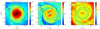Fig. 1. Outcome of the numerical simulation (BLh, 1.00) at 4.6 ms after merger. The left, central, and right panels show the rest mass density, the temperature, and the electron fraction on the equatorial plane, respectively. The black lines mark isodensity contours corresponding to 1012 g cm−3 (solid line), 1013 g cm−3 (dashed line), 1014 g cm−3 (dashed-dotted line), and 1015 g cm−3 (dotted line).

3.2. EOS modelling

In our analysis, we considered baryons, massive leptons, photons, and neutrinos as the relevant d.o.f. to describe matter and radiation in BNS mergers. Baryons, massive leptons, and photons are assumed to be in thermal and nuclear statistical equilibrium everywhere inside the remnant. Nuclear statistical equilibrium is reached when strong and electromagnetic reactions are in equilibrium, and the nuclear composition is provided by the minimum of the free energy. For astrophysically relevant conditions, this is verified as long as k_BT ≳ 0.6 MeV (e.g. Hix & Thielemann 1999). In astrophysical plasma, the negative net charge of massive leptons is balanced by the positive charge of protons. In the presence of more than one massive lepton, charge neutrality implies:

$$\begin{array}{c}\hfill Y_{\mathrm{p}}={\displaystyle \sum _{l=e,\mu ,\tau }{Y}_l,}\end{array}$$(13)

where Y_p = n_p/n_b is the proton fraction; n_p is the proton number density; Y_l = (n_l⁻ − n_l⁺)/n_b is the net fraction of the massive lepton l; and e, μ, and τ stand for electron, muon, and tauon, respectively.

Every relevant species was characterised by its own EOS. These EOSs can be expressed in terms of any thermodynamical potential, such as the Helmholtz free energy F with the volume V, the number of particles N, and the temperature T, as independent variables. Neglecting the modifications of the thermodynamical potentials due to the interaction between different d.o.f., the total free energy was given by

$$\begin{array}{c}\hfill F_{\mathrm{tot}}={\displaystyle \sum _{i=b,l,\gamma ,\nu }{F}_i,}\end{array}$$(14)

where the subscript i = {b, l, γ, ν} indicates baryons, massive leptons, photons, and neutrinos, respectively. All the thermodynamic variables, such as the chemical potentials, μ_i, the energy densities, e_i, and the pressures, P_i, were derived from F_i at fixed temperature T, number of particles N_i, and volume V according to the standard rules of the canonical ensemble. Hence, the total energy density and pressure were simply given by

$$\begin{array}{c}\hfill e_{\mathrm{tot}}={\displaystyle \sum _{i=b,l,\gamma ,\nu }{e}_i,P_{\mathrm{tot}}=\sum _{i=b,l,\gamma ,\nu }{P}_i.}\end{array}$$(15)

In the following sections, we provide a detailed description of the EOSs used in this work for each species.

3.2.1. Baryons

Our knowledge of the baryonic matter EOS is still affected by large uncertainties. Therefore, to bracket possible uncertainties in this work, the baryonic contribution was taken into account via three different nuclear EOSs in tabulated form corresponding to the ones used in the simulations presented in Sect. 3.1: the BLh (Bombaci & Logoteta 2018; Logoteta et al. 2021), the DD2 (Typel et al. 2010; Hempel & Schaffner-Bielich 2010), and the SFHo (Steiner et al. 2013)². We note that we did not consider the possible formation of hyperons (Oertel et al. 2012; Fortin et al. 2018) or a phase transition to quark matter (Weissenborn et al. 2011; Klähn et al. 2013; Chatterjee & Vidaña 2016; Bombaci et al. 2016; Logoteta et al. 2019; Logoteta 2021). The BLh EOS is a microscopic EOS constructed following the framework of the Brueckner-Bethe-Goldstone many-body theory extended at finite temperatures within the Brueckner-Hartree-Fock approximation. In contrast, the modelling of nuclear interactions in DD2 and SFHo is based on a relativistic mean field theory. For each nuclear EOS, the independent variables are (n_b, T, Y_p). The range of (n_b, T, Y_p) for each EOS table is reported in Table 2. The three EOSs are in reasonable agreement with the experimental constraints on the properties of nuclear matter at n₀ and T = 0 (for experimental constraints, see Shlomo et al. 2006; Danielewicz & Lee 2014; Oertel et al. 2017; Drischler et al. 2019). Moreover, all three EOSs satisfy to a good extent present astrophysical constraints on the NS maximum mass M_max > 2.01 M_⊙ and NS radius (Antoniadis et al. 2013; Lattimer & Steiner 2014; Oertel et al. 2017; Riley 2019; Miller et al. 2019, 2021; Raaijmakers et al. 2021).³ In Table 2, we report for each EOS the values of the nuclear saturation density, the maximum mass M_max of a cold non-rotating NS, the corresponding radius R_max, the radius R_1.4 of a 1.4 M_⊙ NS, and the dimensionless tidal deformability $\stackrel{\sim }{\mathrm{\Lambda }}$ (e.g. Hinderer 2008; Damour et al. 2012; Favata 2014) for GW170817 targeted binaries. We note that SFHo supports a smaller maximum NS mass with a smaller radius. More generally, SFHo produces more compact NSs compared to the other two EOSs. In the case of BLh, it predicts slightly larger M_max and R_max, but the values are still close to the ones from SFHo. Conversely, DD2 exhibits significantly larger values for M_max and R_max and a smaller compactness. Despite the fact that the maximum NS properties of SFHo and BLh are relatively close, it is worth noting that for other properties at densities equal to several times n₀, SFHo and DD2, regarding the symmetry energy, and DD2 and BLh, for incompressibility, are more similar. With this selection of baryonic EOSs, we could explore very different microphysical descriptions and a wide range of thermodynamical conditions and macroscopic properties of merging BNSs.

3.2.2. Massive leptons and photons

We treated massive leptons as ideal Fermi gases in thermal equilibrium. In particular, we incorporated electrons and positrons e^± as well as muons and anti-muons μ^±, while we neglected tauons and anti-tauons τ^± due to their large mass compared to the typical temperatures and Fermi energies in the system. The EOS of a non-interacting gas⁴ of fermions at a finite temperature is well known in the literature, and it provides the expressions for the number density n_l^±, the specific energy density e_l^±, and the pressure P_l^± (Bludman & van Riper 1977):

$$\begin{array}{c}\hfill n_{l^{\pm }}=K_l{\theta }_l^{3/2}[F_{1/2}({\eta }_{l^{\pm }}^{\prime },{\theta }_l)+{\theta }_l{F}_{3/2}({\eta }_{l^{\pm }}^{\prime },{\theta }_l)]\end{array}$$(16)

$$\begin{array}{c}\hfill e_{l^{\pm }}=K_l{m}_l{c}^2{\theta }_l^{5/2}[F_{3/2}({\eta }_{l^{\pm }}^{\prime },{\theta }_l)+{\theta }_l{F}_{5/2}({\eta }_{l^{\pm }}^{\prime },{\theta }_l)]+m_l{c}^2{n}_{l^{\pm }}\end{array}$$(17)

$$\begin{array}{c}\hfill P_{l^{\pm }}=\frac{K_l{m}_l{c}^2}{3}{\theta }_l^{5/2}[2F_{3/2}({\eta }_{l^{\pm }}^{\prime },{\theta }_l)+{\theta }_l{F}_{5/2}({\eta }_{l^{\pm }}^{\prime },{\theta }_l)],\end{array}$$(18)

where m_l is the lepton mass and K_l is a constant

$$\begin{array}{c}\hfill K_l=8\sqrt{2}\pi {(m_l{c}^2/hc)}^3,\end{array}$$(19)

θ_l and ${\eta }_{l^{\pm }}^{\prime }$ are the relativity and the non-relativistic degeneracy parameters, respectively,

$$\begin{array}{c}\hfill {\theta }_l=\frac{k_{\mathrm{B}}T}{m_l{c}^2},{\eta }_{l^{\pm }}^{\prime }=\frac{{\mu }_{l^{\pm }}-m_l{c}^2}{k_{\mathrm{B}}T},\end{array}$$(20)

while $F_k({\eta }_{l^{\pm }}^{\prime },{\theta }_l)$ are the generalised Fermi functions of order k. At thermal equilibrium, the degeneracy parameter of anti-particles ${\eta }_{l^{+}}^{\prime }$ is related to that of particles ${\eta }_{l^{-}}^{\prime }$ (Timmes & Arnett 1999):

$$\begin{array}{c}\hfill {\eta }_{l^{+}}^{\prime }=-({\eta }_{l^{-}}^{\prime }+2\frac{m_l{c}^2}{k_{\mathrm{B}}T}).\end{array}$$(21)

By inverting Eq. (16), the term ${\eta }_{l^{-}}^{\prime }$ can be expressed as a function of (n_b, Y_l, T), as was suggested in Timmes & Arnett (1999).

Photons form an ideal Bose gas in thermal equilibrium with matter and with zero chemical potential, μ_γ = 0. The resulting EOS of photons depends only on T:

$$\begin{array}{c}\hfill n_{\gamma }=\frac{16\pi k_{\mathrm{B}}^3\zeta (3)}{{(hc)}^3}{T}^3,e_{\gamma }=\frac{8{\pi }^5{k}_{\mathrm{B}}^4}{15{(hc)}^3}{T}^4,\end{array}$$(22)

and P_γ = e_γ/3.

3.2.3. Trapped neutrinos

Based on the discussion in Sect. 2 and as typical neutrino energies inside the remnant are much larger than any neutrino mass, we modelled the trapped neutrino component as a massless Fermi gas in weak and thermal equilibrium with matter and radiation. Accordingly, the particle number density n_ν, the energy density e_ν, and the pressure P_ν of any flavour neutrino ν were given by

$$\begin{array}{c}\hfill n_{\nu }=\frac{4\pi }{{(hc)}^3}{\left(k_{\mathrm{B}}T\right)}^3{F}_2({\eta }_{\nu })e^{-({\rho }_{\lim }/\rho )},\end{array}$$(23)

$$\begin{array}{c}\hfill e_{\nu }=\frac{4\pi }{{(hc)}^3}{(k_{\mathrm{B}}T)}^4{F}_3({\eta }_{\nu })e^{-({\rho }_{\lim }/\rho )},\end{array}$$(24)

$$\begin{array}{c}\hfill P_{\nu }=e_{\nu }/3,\end{array}$$(25)

where the exponential factor e^{−(ρ_lim/ρ)} was introduced in order to model the fading of the trapped component at ρ ≲ ρ_lim (see also Kaplan et al. 2014 and Perego et al. 2019 for a similar choice). The degeneracy parameter of anti-neutrinos was fixed by ${\eta }_{\overline{\nu }}=-{\eta }_{\nu }$ because of thermal equilibrium. Furthermore, η_ντ = 0 since the fraction of tauons is negligible, while weak equilibrium defined the degeneracy parameters of electronic and muonic neutrinos:

$$\begin{array}{c}\hfill {\eta }_{{\nu }_l}={\eta }_{\mathrm{p}}^{\prime }(n_b,Y_{\mathrm{p}},T)-{\eta }_{\mathrm{n}}^{\prime }(n_b,Y_{\mathrm{p}},T)+{\eta }_{l^{-}}^{\prime }(n_b,Y_l,T)\\ \hfill +\frac{(m_{\mathrm{p}}-m_{\mathrm{n}}+m_l)c^2}{k_{\mathrm{B}}T}(l=e,\mu ),\end{array}$$(26)

where ${\eta }_{\text{n}}^{\prime }$ and ${\eta }_{\text{p}}^{\prime }$ are the non-relativistic degeneracy parameters of neutrons and protons, respectively. Accordingly, the EOS of electron (muon) neutrinos depends on T, Y_p, and Y_e (Y_μ), while the EOS of tauon neutrinos depends only on T and does not distinguish between ν_τ and ${\overline{\nu }}_{\tau }$. The fraction of neutrinos and their mean energy were defined as Y_ν = n_ν/n_b and E_ν = e_ν/n_ν, respectively.

From the previous discussion, if all the species are assumed to be in thermal and reaction equilibrium, the set of variables needed to describe the complete EOS is given by (n_b, T, Y_p, Y_e, Y_μ). However, the charge neutrality of NS matter constrains the proton fraction Y_p = Y_e + Y_μ, reducing the set of independent variables to (n_b, T, Y_e, Y_μ).

3.3. The post-processing technique

Based on the simulation outcome discussed in Sect. 3.1, we estimated the amount and the impact of muons in post-processing as well as their influence on the trapped neutrino properties. In particular, we were interested in the implications for the remnant on a timescale Δt ∼ 5 − 15 ms after the merger and in the density region ρ ≳ 10¹³ g cm⁻³ where the approximation of weak and thermal equilibrium better applies. The absence of muons inside the original simulations posed a significant issue and required some modelling (shown in Sect. 3.3.1) before the post-processing technique could be applied (discussed in Sect. 3.3.2).

3.3.1. Modelling

We modelled the NS fluid elements before the merger as being composed of neutrons, protons, electrons, and muons in cold neutrinoless weak equilibrium:

$$\begin{array}{c}\hfill \{\begin{array}{cc}{\mu }_{\mathrm{e}}(T=0)\hfill & ={\mu }_n(T=0)+{\mu }_p(T=0)\hfill \\ {\mu }_{\mu }(T=0)\hfill & ={\mu }_{\mathrm{e}}(T=0).\hfill \end{array}\end{array}$$(27)

In Fig. 2, we show the fractions of electrons, muons, and protons as a function of n_b, obtained by solving Eq. (27). At n_b ≈ 0.3fm⁻³ ∼ 2 n₀, the muon fraction is approximately 40% of the electron fraction for all the considered EOSs, and it increases monotonically with n_b. For comparison, we also show the electron fraction calculated by assuming β-equilibrium without muons (see dashed black line in Fig. 2), which corresponds to the initial conditions used in the simulations presented in Sect. 3.1. A common feature of all three models is that when muons are included, the electron fraction becomes smaller, while the proton fraction tends to increase, that is, Y_p = Y_e + Y_μ. In particular, the system lowers the Fermi energy of electrons by converting electrons into muons up to the point where the chemical potentials of electrons and muons are equal, balancing the difference between the neutron and proton chemical potentials. Moreover, when muons are included, neutrons can turn into protons plus muons via Urca processes (Leinson 2002; Yakovlev & Pethick 2004; Potekhin et al. 2015). The three EOSs show pronounced differences in the density behaviour of the electron fraction. In particular, BLh predicts a higher Y_p at large densities compared to DD2 and SFHo. Such differences are mainly due to the different density behaviours of the symmetry energy in the three models. Symmetry energy is indeed the principal source that determines matter composition at a given density and temperature. In the following paragraphs, we refer to the particle fractions of the cold NSs obtained by solving Eq. (27) as ${\stackrel{\sim }{Y}}_{\mathrm{e}}(n_b)$ and ${\stackrel{\sim }{Y}}_{\mu }(n_b),$ which are represented as solid lines in Fig. 2, and to the net electron fraction computed in cold weak equilibrium without muons (see dashed black line in Fig. 2) as ${\stackrel{\sim }{Y}}_{\mathrm{e},0}(n_b)$.

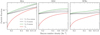Fig. 2. Particle fractions computed at T = 0 in neutrinoless β-equilibrium for three different EOS: BLh (left), DD2 (centre), and SFHo (right). Black lines show the electron fraction computed in two different cases: equilibrium with muons (solid lines) or without muons (dashed lines). The green line corresponds to the fraction of protons at equilibrium with muons, while the red line corresponds to the muon fraction. We note that when muons are not included, the proton fraction coincides with the electron one (dashed black line).

During a merger, the density, temperature, and composition of the fluid elements change because of matter compression and decompression, and neutrinos are produced. If a fluid element is in good approximation within the last scattering neutrino surface (i.e. ρ ≳ ρ_lim), a trapped neutrino gas is formed in weak and thermal equilibrium with matter. In these conditions, it is convenient to introduce for each fluid element the electron, muon, and tauon lepton numbers

$$\begin{array}{c}\hfill Y_{l,j}=Y_j+Y_{{\nu }_j}-Y_{{\overline{\nu }}_j}j=\{e,\mu ,\tau \},\end{array}$$(28)

and the total fluid energy

$$\begin{array}{c}\hfill e_{\mathrm{tot}}={\displaystyle \sum _i{e}_{i}i=\{b,e^{\pm },{\mu }^{\pm },\gamma ,{\nu }_j,{\overline{\nu }}_j\}.}\end{array}$$(29)

The central part of the remnant, characterised by ρ ≳ 10¹⁴ g cm⁻³, is formed by the fusion of the two NSs cores, and it is characterised by fluid elements whose density is significantly in excess of the neutrino surface density during their evolution. Such fluid elements are not affected by shocks and significant neutrino emission. In particular, as discussed in Sect. 2, the neutrino diffusion timescale, t_diff, is in the order of seconds; thus t_diff ≫ Δt ∼ 5 − 15 ms (see Eq. (11)). So these fluid elements conserve their electron and muon lepton fractions over Δt, which are ultimately equal to the electron and muon lepton fractions set by the initial cold neutrinoless equilibrium, Eq. (27)⁵ A close inspection of the thermodynamic conditions experienced by matter in a BNS merger event and of their corresponding evolution (Perego et al. 2019) revealed that the conservation of the lepton numbers is well realised for matter originally inside the outer core of the two cold NSs, that is, at ρ ≳ 10¹⁴ g cm⁻³ also during the inspiral. In contrast, most of the matter at a lower density inside the merger remnant, ρ < 10¹⁴g cm⁻³, originates from the decompression of matter originally around ρ ∼ 10¹⁴ g cm⁻³ inside the two merging NSs. In this case, matter is significantly heated by shocks and compression such that the electron and muon lepton numbers of each fluid element become considerably altered. In this density domain, the electron fraction evolved through the numerical relativity simulations is a better proxy of Y_l, e: $Y_{l,e}\sim Y_{\mathrm{e}}^{\mathrm{sim}}$. The muon lepton fraction is instead approximately given by Y_l, μ ∼ 0.01, which corresponds to the typical muon fraction in the original NSs at the edge of the outer core, that is, around and just below saturation density (see Fig. 2).

Concerning the relativistic internal energy, no significant energy leaks out in the form of neutrinos from the fluid elements until t_diff ≫ Δt in neutrino trapping conditions. Thus, the evolution of e_sim inside the simulation is also expected to reproduce in good approximation the evolution (i.e. the variation) of the total internal energy once muons and neutrinos are present. However, the presence of physical muons inside the two cold NSs alters the absolute value of the relativistic internal energy due to their rest mass contribution. Nevertheless, this contribution remains approximately constant in time as long as the bulk of the muons present in the remnant comes from the two cold NSs.

3.3.2. Algorithm

Based on the above considerations, we designed the following post-processing algorithm. We considered the time snapshots of the simulations listed in Table 1 in the time interval ∼5 − 15 ms. From each snapshot, we read the full 3D profile of the baryon number density $n_b^{\text{sim}}$, the net electron fraction $Y_{\mathrm{e}}^{\mathrm{sim}}$, and the internal energy density e_sim on a Cartesian grid (x, y, z) with −30 km ≤ x, y, z ≤ +30 km. Given $(n_b^{\mathrm{sim}},Y_{\mathrm{e}}^{\mathrm{sim}},e_{\mathrm{sim}})$ on the Cartesian grid and for each snapshot, we performed our analysis according to the following steps.

Given $Y_{\mathrm{e}}^{\mathrm{sim}}$, we computed the baryon density ${\overline{n}}_b$ such that $Y_{\mathrm{e}}^{\mathrm{sim}}={\stackrel{\sim }{Y}}_{\mathrm{e},0}({\overline{n}}_b).$ (See Sect. 3.3.1 and dashed black line in Fig. 2.) We note that ${\overline{n}}_b$ corresponds to the original density of the fluid element inside the NSs during the inspiral, and it is, in general, different from $n_b^{\text{sim}}$.

We computed the cold equilibrium electron and muon net fractions corresponding to ${\overline{n}}_b$ (i.e. ${\stackrel{\sim }{Y}}_{\mathrm{e}}({\overline{n}}_b)$ and ${\stackrel{\sim }{Y}}_{\mu }({\overline{n}}_b)).$ (See Sect. 3.3.1 and solid black and red lines in Fig. 2.)

Given the simulation baryon number density $n_b^{\text{sim}}$, we computed ${\rho }_{\text{sim}}=m_{\text{amu}} n_b^{\text{sim}}$. If ρ_sim > 10¹⁴ g cm⁻³, then the lepton numbers were separately conserved (see discussion in Sect. 3.3.1). Therefore, we identified the electron and muon lepton fractions with

$$\begin{array}{c}\hfill Y_{l,\mathrm{e}}={\stackrel{\sim }{Y}}_{\mathrm{e}}({\overline{n}}_b)Y_{l,\mu }={\stackrel{\sim }{Y}}_{\mu }({\overline{n}}_b).\end{array}$$(30)

If instead ρ_sim < 10¹⁴ g cm⁻³, we imposed

$$\begin{array}{c}\hfill Y_{l,\mathrm{e}}=Y_{\mathrm{e}}^{\mathrm{sim}}{Y}_{l,\mu }=0.01.\end{array}$$(31)

In accordance with our assumptions, Y_l, τ = 0 everywhere and at any time. We note that the proton fraction (which in the simulation is equal to $Y_{\mathrm{e}}^{\mathrm{sim}}$) is now larger than $Y_{\mathrm{e}}^{\mathrm{sim}}$ since ${\stackrel{\sim }{Y}}_{\mathrm{p}}={\stackrel{\sim }{Y}}_{\mathrm{e}}+{\stackrel{\sim }{Y}}_{\mu }$.

Given the simulation energy e_sim, if ρ_sim > 10¹⁴ g cm⁻³, we computed the total internal energy density of each fluid element as

$$\begin{array}{c}\hfill e_{\mathrm{tot}}=e_{\mathrm{sim}}+{\stackrel{\sim }{Y}}_{\mu }({\overline{n}}_b)n_b^{\mathrm{sim}}{m}_{\mu }{c}^2,\end{array}$$(32)

while if ρ_sim < 10¹⁴ g cm⁻³, we computed

$$\begin{array}{c}\hfill e_{\mathrm{tot}}=e_{\mathrm{sim}}+0.01n_b^{\mathrm{sim}}{m}_{\mu }{c}^2.\end{array}$$(33)

The terms proportional to $n_b^{\text{sim}}{m}_{\mu }{c}^2$ correspond to the rest mass energy density of the muons already present in the two cold NSs.

We imposed $n_b=n_b^{\text{sim}}$, and we solved the system

$$\begin{array}{cc}\hfill Y_{l,e}& =Y_{\mathrm{e}}+Y_{{\nu }_{\mathrm{e}}}(n_b,T,Y_{\mathrm{e}},Y_{\mu })-Y_{{\overline{\nu }}_{\mathrm{e}}}(n_b,T,Y_{\mathrm{e}},Y_{\mu })\hfill \\ \hfill Y_{l,\mu }& =Y_{\mu }+Y_{{\nu }_{\mu }}(n_b,T,Y_{\mathrm{e}},Y_{\mu })-Y_{{\overline{\nu }}_{\mu }}(n_b,T,Y_{\mathrm{e}},Y_{\mu })\hfill \\ \hfill e_{\mathrm{tot}}& ={\displaystyle \sum _i{e}_i(n_b,T,Y_{\mathrm{e}},Y_{\mu }),}\hfill \end{array}$$(34)

with respect to (T, Y_e, Y_μ), where $i=\{b,e^{\pm },{\mu }^{\pm },\gamma ,{\nu }_j,{\overline{\nu }}_j\}$ and j = {e, μ, τ}, to find the equilibrium configuration in the presence of (anti)muons and trapped neutrinos. The (anti-)neutrino fractions, Y_ν, and energies, e_ν, are defined in Sect. 3.2.3. We note that the condition on the tauon lepton number, Y_l, τ = 0, is automatically satisfied in the absence of physical tauons and by the resulting η_ντ = 0 assumption. Nevertheless, the contribution of tauon (anti-)neutrinos was taken into account in the calculation of the total energy and pressure.

We computed all the other thermodynamic variables, such as fractions of trapped neutrinos, chemical potentials, and pressures as functions of (n_b, T, Y_e, Y_μ), as prescribed in Sect. 3.2.

We note that in our procedure, we did not prescribe any time evolution. Rather, we post-processed each available time snapshot of the original simulation in the interval ∼5 − 15 ms after merger.

3.3.3. Limits of validity

Our post-processing analysis allowed us to compute, a posteriori, the thermodynamics of the merger aftermath taking into account the presence of muons and trapped neutrinos. We note that since there are no muons nor any explicit neutrinos in the original simulations, the definition of Y_l, e, Y_l, μ, and e_tot based on the simulation outcome cannot be done in a unique and fully consistent way. The choice described in the previous paragraph has the advantage of including the contribution given by the muons already present in the cold NSs. However, it relies on the assumption that the merger dynamics and e_sim, once corrected for the muons rest mass energy, are not significantly altered by them. To bracket the uncertainties due to this choice, in Appendix A, we discuss our results for a different choice of Y_l, e, Y_l, μ, and e_tot where the initial muon fraction from the cold NSs is neglected.

In our modelling of neutrinos, we assumed that above ρ_lim, e, there is a full Fermi-Dirac distribution of trapped neutrinos. However, neutrinos with energy smaller than 10 − 20 MeV were not expected to be in equilibrium with matter in this density regime. Moreover, from Eq. (12) it follows that the diffusion timescale of neutrinos with energy E_ν ∼ 15 MeV becomes comparable to Δt ∼ 10 ms around ρ ∼ 10¹² g cm⁻³. For this reason, even though we applied our post-processing procedure in the density domain ρ > ρ_lim, e, we restricted our analysis of the results to ρ > 10¹³ g cm⁻³, where the assumption of neutrino trapping and weak equilibrium is robust, being t_diff ≫ t_dyn, and the post-processing approach is more reliable, being t_diff ≫ Δt. We also note that our modelling of the trapped neutrino component closely follows the one used by Perego et al. (2019). Recent numerical results obtained by including neutrino transport through a grey M1 moment scheme in BNS merger simulations (Zappa et al. 2023) are very consistent with the outcome of the post-processing analysis of Perego et al. (2019).

Finally, we highlight that in our procedure, the population of anti-muons is given by a Fermi-Dirac distribution in thermal equilibrium. Therefore, anti-muons arise as a thermal tail at a high enough temperature.

4. The fraction of muons in the remnant

We started our post-processing analysis from the simulation (BLh, 1.00). In Fig. 3, we show the fractions of μ^±, ν_μ, and ${\overline{\nu }}_{\mu }$ as well as the muon chemical potential approximately 5 ms after merger. The fraction of muons, Y_μ⁻, is ∼0.01 − 0.07 in the high-density region characterised by ρ > 10¹⁴ g cm⁻³, while it decreases down to ∼10⁻³ − 10⁻² at the lower density ρ ∼ 10¹³ − 10¹⁴ g cm⁻³. By computing the difference $Y_{{\mu }^{-}}-{\stackrel{\sim }{Y}}_{\mu }$ (upper-right panel of Fig. 3 ), we deduced that the bulk of muons comes from the two cold NSs. This result is consistent with the hypothesis of our post-processing procedure (see Sect. 3.3.1). However, a fraction of the muons was created during the merger, corresponding to ∼10⁻³ − 10⁻². Muon creation became enhanced in correspondence to the hot spots where k_BT_sim ≳ 50 MeV (see the second panel of Fig. 1) and at high density, that is, above 10¹⁵ g cm⁻³. By inspecting the change in temperature and particle fractions

$$\begin{array}{c}\hfill \mathrm{\Delta }T=T-T_{\mathrm{sim}}\mathrm{\Delta }{Y}_i=Y_i-Y_i^{\mathrm{sim}},\end{array}$$(35)

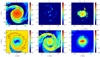Fig. 3. Particle fractions and chemical potential in the muon flavour sector computed by post-processing the simulation (BLh, 1.00) at 4.6 ms after merger. In the upper panels, we show the fraction of μ− (left), the fraction of μ+ (centre), and the difference between the muon fraction and the one inherited from the cold NSs, that is, $Y_{{\mu }^{-}}-{\stackrel{\sim }{Y}}_{\mu }$ (right). In the lower panels, we show the fraction of νμ (left), the fraction of ${\overline{\nu }}_{\mu }$ (centre), and the muon chemical potential (rest mass subtracted) (right). As in Fig. 1, the black lines mark isodensity contours.

where T and Y_i result from post-processing calculations, while T_sim and $Y_i^{\text{sim}}$ are read from the simulation, we could guess which were the processes more likely to be involved in muon creation. In the hot spots, both muons and anti-muons were produced, and the fraction of newly created muons Y_μ⁻ ∼ 10⁻² exceeded the fraction of anti-muons Y_μ⁺ ∼ 10⁻³ (see Fig. 3, upper-centre and right panels). At the same time, we observed ΔT < 0, ΔY_n < 0 and ΔY_e⁻ > 0. We concluded that, on the one hand, thermal processes drive the creation of μ^± pairs at the expense of the system’s internal energy, and on the other hand, the reduction in the degeneracy of muons due to the high temperature (see Fig. 3, lower-right panel) favours the conversion of n into p + μ⁻, further enhancing the production of μ⁻. In addition, we found an enhancement in the creation of e^± pairs and e⁻, but the amount of newly created μ⁻ systematically exceeded that of the newly created e⁻. In the core of the remnant, the density of fluid elements was enhanced by matter compression, and μ⁻ as well as e⁻ were created at the expense of the neutrons’ degeneracy (ΔY_n < 0). Finally, at a lower density, ρ < 10¹⁴ g cm⁻³, the initial muon fraction from cold, decompressing NSs matter was almost entirely converted into muon neutrinos. We note that the values of Y_μ⁻ are stable in the time domain of our analysis.

Next, we compare the results obtained from the simulation (BLh, 1.00) with the ones from (DD2, 1.00) and (SFHo, 1.00). In the latter cases, muons were also present in the full-density region, ρ > 10¹³ g cm⁻³. However, the muon fraction Y_μ⁻ ∼ 10⁻³ − 0.05 presented a slightly smaller maximum with respect to (BLh, 1.00). This is expected since, as discussed in Sect. 3.3.1, DD2 and SFHo predict a smaller muon fraction for cold nuclear matter in weak equilibrium (see also Fig. 2). The amount of muons created during the merger (i.e. $Y_{{\mu }^{-}}-{\stackrel{\sim }{Y}}_{\mu })$ is comparable for the three simulations and correlates in the same way with ΔT and ΔY_i, defined in Eq. (35). The amount of μ⁻ and ${\overline{\nu }}_{\mu }$ produced in the centre of the remnant, however, was smaller for (DD2, 1.00) and (SFHo, 1.00) with respect to (BLh, 1.00), with a difference that can reach one order of magnitude if we compare (DD2, 1.00) to (BLh, 1.00). As in the case of the cold, neutrinoless weak equilibrium conditions presented in Fig. 2, such a difference between the BLh EOS and the DD2 EOS is mostly due to the larger slope of the symmetry energy in the former case. Additionally, the fraction of μ⁻ was on average slightly larger in (SFHo, 1.00) than in (DD2, 1.00) because the softer EOS SFHo exhibits larger temperatures and densities than the stiffer DD2 EOS (see e.g. Foucart et al. 2016a; Sekiguchi et al. 2016; Radice et al. 2018a; Perego et al. 2019).

To assess the relevance of muons in the merger remnants, we compared the equilibrium net muon fraction obtained in our post-processing procedure with the equilibrium net electron fraction by analysing the ratio Y_μ/Y_e, as shown in Fig. 4. We note that for all the simulations, the net muon fraction was at least 30%−40% of the net electron fraction. The ratio Y_μ/Y_e was the largest for (BLh, 1.00), where it can reach a maximum of approximately 0.7, while it reached up to 0.6 and 0.5 for (SFHo, 1.00) and (DD2, 1.00), respectively. We stress, however, that due to the large mass difference between electrons and muons, the amount of both electrons and positrons was largely increased where the temperature was high such that Y_e⁻ ≳ Y_e⁺ and Y_e = Y_e⁻ − Y_e⁺ ∼ 0.1, while Y_μ⁻ ≫ Y_μ⁺ and Y_μ ≈ Y_μ⁻.

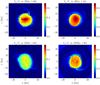Fig. 4. Ratio of the net muon fraction over the net electron fraction, Yμ/Ye, on the equatorial plane obtained by post-processing simulations (BLh, 1.00) (upper left), (BLh, 1.43) (upper right), (DD2, 1.00) (lower left), and (SFHo, 1.00) (lower right) at 5 − 6 ms after merger. As in Fig. 1, the black lines mark isodensity contours.

Finally, we post-processed data from the simulation (BLh, 1.43), which had a significantly larger mass asymmetry. We did not observe notable differences while comparing the maximum value of Y_μ/Y_e in (BLh, 1.00) and (BLh, 1.43). However, (BLh, 1.43) exhibited a more extended spatial region where Y_μ/Y_e ∼ 0.5 − 0.6 (see Fig. 4). This region is characterised by a large temperature, ≳40 MeV, because it embeds the core of the secondary NS, which was broadened and strongly heated by compression and shocks during the merger.

5. Trapped neutrino properties

In Figs. 3 and 5, we show all flavour (anti-)neutrino abundances as well as the chemical potentials of baryons and massive leptons computed by post-processing the simulation (BLh, 1.00) at approximately 5 ms after merger. Trapped gases of (anti-)neutrinos were present in the full-density regime of our analysis, ρ > 10¹³ g cm⁻³, but the abundances and the species hierarchy varied according to the system density and temperature.

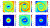Fig. 5. Fractions of νe, ${\overline{\nu }}_{\mathrm{e}}$, ντ, and chemical potentials of electrons, protons, and neutrons computed in post-processing for (BLh, 1.00) at 4.6 ms after merger. In the upper panels, we show the fraction of νe (left), the fraction of ${\overline{\nu }}_{\mathrm{e}}$ (centre), and the fraction of ντ (right). In the lower panels, we show the electron chemical potential (rest mass subtracted) μe − me (left), the proton chemical potential (rest mass subtracted) μp − mp (centre), and the neutron chemical potential (rest mass subtracted) μn − mn (right). We note that the colour bar scales are different for the various chemical potentials. As in Fig. 1, the black lines mark the isodensity contours.

In the very-high-density regime, ρ ≳ 7 × 10¹⁴ g cm⁻³, ν_e and ν_μ were suppressed (Y_νe, μ < 10⁻⁴), while ${\overline{\nu }}_{\mathrm{e}}$ and ${\overline{\nu }}_{\mu }$ had typical fractions $Y_{{\overline{\nu }}_{\mathrm{e},\mu }}\sim {10}^{-3}-{10}^{-2}$, with ${\overline{\nu }}_{\mu }$ being slightly more abundant than ${\overline{\nu }}_{\mathrm{e}}$. We note that the excess of ${\overline{\nu }}_{\mathrm{e}}$ and ${\overline{\nu }}_{\mu }$ exactly compensates for the amount of newly created electrons and muons (see the discussion in the previous section). Among the remaining neutrino species, ν_τ and ${\overline{\nu }}_{\tau }$ were the most abundant, with a fraction ∼10⁻⁴ − 10⁻³.

When ρ ∼ 2 − 6 × 10¹⁴ g cm⁻³, the fractions of neutrinos increased up to ∼10⁻³, but electron and muon anti-neutrinos still remained the most abundant neutrino species, with $Y_{{\overline{\nu }}_{\mathrm{e},\mu }}\sim {10}^{-3}-0.02$. All the (anti-)neutrino abundances peaked in the hot spots. However, muon production dominated in this density and temperature regime (see the discussion in the previous section) so that the ${\overline{\nu }}_{\mu }$ species was the most abundant, followed by ${\overline{\nu }}_{\mathrm{e}}$ and then ν_τ, ν_e, and ν_μ, in that order.

At the lower density, ρ ∼ 10¹³ − 10¹⁴ g cm⁻³, all neutrinos and anti-neutrinos were present in warm matter streams characterised by k_BT_sim ∼ 25 MeV, with order of magnitude fractions ∼10⁻², and the ${\overline{\nu }}_{\mathrm{e}}$ species dominated, followed in order by ${\overline{\nu }}_{\mu }$, ν_τ, ν_μ, and ν_e. On the contrary, in cold matter streams with k_BT_sim ∼ 10 − 15 MeV, anti-neutrinos were suppressed, and the ν_μ species dominated, with a maximum fraction of ∼0.01, followed by ν_e, with Y_νe ≳ 10⁻³, and ν_τ, with Y_ντ ∼ 10⁻⁴.

The different abundances and the hierarchy reflect the behaviour of the neutrino chemical potentials at equilibrium (see Eq. (26)), which ultimately depend on the EOS both directly, through the nuclear interaction, and indirectly, through the different thermodynamic conditions realised in the remnant. The regions where anti-neutrinos dominated over neutrinos were characterised by a higher density and a higher value of the neutron chemical potential μ_n, which exceeded μ_p + μ_l⁻ with l = {e, μ}, as we deduced from Figs. 3 and 5. In such regions, the density was increased by matter compression, and the fraction of protons increased as well since the lepton number was fixed. This coincided with the enhancement of electrons and muon production at the expense of free neutrons (see discussion in Sect. 4), and the equilibrium condition Eq. (26) enforced the creation of the corresponding anti-neutrinos. In contrast, neutrinos dominated in relatively cold matter streams in the outer layers, where the proton chemical potential increased (see Fig. 5) so that μ_p + μ_l⁻ > μ_n. The enhancement of μ_p is indeed correlated with the decrease of both density and temperature experienced by the expanding matter in such regions. This is illustrated in Fig. 6, where we plotted μ_p and μ_n in the ρ − T plane for Y_p fixed to a relevant value for the analysis (i.e. Y_p = 0.08). We note that μ_p started increasing when ρ ≲ 10¹⁴ g cm⁻³ and k_BT ≲ 15 MeV, while μ_n decreased in the same ρ − T region. This is because when ρ ≲ 10¹⁴ g cm⁻³ and k_BT ≲ 15 MeV, nucleons start clustering in nuclei so that the chemical potential of free protons is enhanced and the amount of free protons drops (see e.g. Fig. 8 of Hempel & Schaffner-Bielich 2010). At a fixed lepton fraction and at equilibrium, this results in a conversion of electrons and muons into the corresponding neutrinos.

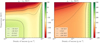Fig. 6. Proton and neutron chemical potentials (rest mass subtracted) of BLh in the density-temperature plane at fixed Yp = 0.08. The proton fraction Yp = 0.08 is the equilibrium proton fraction at 4.6 ms after merger around the point x = 0.64 km, y = 12.76 km, z = 0 km, where ρ ∼ 5 × 1013 g cm−3, Tsim ∼ 10 MeV, and neutrinos dominate, while anti-neutrinos are suppressed (see also Figs. 1, 3 and 5). We notice that the colour bars are scaled differently.

The properties of the neutrino gases are better characterised in terms of their degeneracy parameters. In Fig. 7, we show the degeneracy parameter of electron and muon neutrinos computed for three snapshots of (BLh, 1.00): ∼5 ms, ∼7 ms, and ∼12 ms after merger. The spatial distribution of η_νe and η_νμ clearly indicates the presence of trapped degenerate gases of the ${\overline{\nu }}_{\mathrm{e}}$ and ${\overline{\nu }}_{\mu }$ species in the remnant core and of the ν_e and ν_μ species in the outer layers. In this latter region, the trapped gas of electron neutrinos is characterised by a degeneracy parameter η_νe ranging between three and six, while in the remnant core degenerate electron antineutrinos have ${\eta }_{{\overline{\nu }}_{\mathrm{e}}}=-{\eta }_{{\nu }_{\mathrm{e}}}\sim 4$. The degenerate gases of muonic neutrinos (in the outer layers) and muonic antineutrinos (in the core) exhibited the same qualitative behaviour as the ν_e and ${\overline{\nu }}_{\mathrm{e}}$ species, with a degeneracy parameter η_νμ ranging between -4 and 9 so that these muon (anti-)neutrino gases were slightly more degenerate than the electron ones.

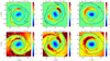Fig. 7. Degeneracy parameter of νe (first row) and νμ (lower row) on the equatorial plane obtained by post-processing the simulation (BLh, 1.00). Three different time slices are shown corresponding from left to right to 4.6 ms, 6.7 ms, and 11.8 ms after merger. As in Fig. 1, the black lines mark the isodensity contours as in Fig. 1.

The spatial distribution of the abundances as well as the neutrino hierarchy in (DD2, 1.00) and (SFHo, 1.00) are fully analogous to the ones of (BLh, 1.00). Accordingly, we can analyse the differences among the three EOSs by inspecting the degeneracy parameters. Similarly to (BLh, 1.00), ${\overline{\nu }}_{\mathrm{e}}$ and ${\overline{\nu }}_{\mu }$ formed degenerate trapped gases in the remnant core, while ν_e and ν_μ formed degenerate trapped gases in the cold matter streams of the outer layers. The degeneracy parameter of electron neutrinos, η_νe, ranged between −2 and 6 for both (DD2, 1.00) and (SFHo, 1.00), while in the case of muonic neutrinos, we found η_νμ ranging between −2 and 11 for (DD2, 1.00) and between −2 and 12 for (SFHo, 1.00). In general, the gases of ${\overline{\nu }}_{\mathrm{e}}$ and ${\overline{\nu }}_{\mu }$ are more degenerate for (BLh, 1.00) than for (DD2, 1.00) and (SFHo, 1.00). The main cause of this resides in the differences among the neutron and the proton chemical potentials, which depend on the selected EOS and on the values of ρ, T, and Y_p in the remnant core. In particular, the average values of ${\mu }_{\text{n}}^{\prime }-{\mu }_{\text{p}}^{\prime }$ (rest masses subtracted) at a radius of approximately 3 km from the centre of the remnants correspond to ∼200 MeV for DD2, ∼245 MeV for SFHo, and ∼325 MeV for BLh. Hence, the degeneracy of the trapped anti-neutrinos is comparable for DD2 and SFHo but quite different for BLh (see Eq. (26)). In this sense, anti-neutrino trapping in the core of the remnant shows a significant and non-trivial dependence on the EOS through the nucleons’ chemical potentials. If the merger dynamics are significantly affected, this characteristic could become a probe for investigating matter properties in the high-density regime.

Finally, by post-processing the results of the simulation (BLh, 1.43), we observed that the degeneracy of the trapped component of anti-neutrinos was the same as in (BLh, 1.00). However, the trapped neutrino gases at ρ ∼ 10¹³ − 10¹⁴ g cm⁻³ were less degenerate for q = 1.43, displaying η_νe ∼ 4 and η_νμ ∼ 7. This feature depends mostly on the temperature in the density region 10¹³ − 10¹⁴ g cm⁻³, which is systematically larger in the case of q = 1.43 compared to q = 1.00.

To test the validity of the approximations used in Sect. 2 and to further characterise the properties of neutrinos trapped inside the remnant in the presence of muons for the first time, we computed the neutrino mean energies, E_ν, in post-processing. In Fig. 8, we show the spatial distribution of E_ν for the remnant of simulation (BLh, 1.00) at approximately 5 ms after merger. In the density region ρ > 10¹³ g cm⁻³, we found E_ν > 30 MeV for all flavour neutrinos, unless a certain flavour was suppressed in a portion of space. Electron and muon anti-neutrinos were the most energetic, with $E_{{\overline{\nu }}_{\mathrm{e},\mu }}\lesssim 180$ MeV. Then, for ν_τ we found E_ντ ≲ 170 MeV, while ν_e and ν_μ were the least energetic, with E_νe, μ ≲ 160 MeV. In the case of (DD2, 1.00), the values of E_ν closely followed the ones discussed for (BLh, 1.00). However, (SFHo, 1.00) exhibited larger energies for all flavour neutrinos, with E_{νe, μ, τ} ≲ 180 MeV and $E_{{\overline{\nu }}_{\mathrm{e},\mu }}\lesssim 200$ MeV, due to larger remnant temperatures.

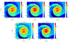Fig. 8. Mean energy Eν of trapped neutrinos on the equatorial plane computed by post-processing simulation (BLh, 1.00) at 4.6 ms after merger. As in Fig. 1., the black lines mark isodensity contours.

6. Changes in the remnant pressure

In this section, we investigate how the result of the post-processing, which consistently included muons and trapped neutrinos, modifies the pressure of the remnant with respect to the values extracted from the original simulation. In Fig. 9, we show the ratio between the pressure computed in post-processing and the simulation pressure, P/P_sim, for (BLh, 1.00), (DD2, 1.00), and (SFHo, 1.00). Similar to Sect. 4 and Sect. 5, we start our discussion with the (BLh, 1.00) simulation. In the time domain of our analysis, the equilibrium pressure computed in post-processing decreased by 6 − 7% in the region characterised by ρ ∼ 5 × 10¹⁴ g cm⁻³, while it increased by a maximum of 3% around 10 km from the centre at ρ ∼ 10¹⁴ g cm⁻³ compared to the pressure from the original simulation.

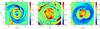Fig. 9. Pressure ratio P/Psim for (BLh, 1.00) (left), (DD2, 1.00) (centre), and (SFHo, 1.00) (right) where P is obtained in post-processing, while Psim is the simulation pressure. For (BLh, 1.00), we explicitly mark the maximum P/Psim ∼ 1.03 (white circle) and the minimum P/Psim ∼ 0.94 (white cross) at ρ > 1014 g cm−3. As in Fig. 1., the black lines mark isodensity contours.

To understand which processes are responsible for the changes in pressure, we analysed the role of each particle species in detail. In Fig. 10, we have plotted the difference in pressures and particle fractions after muons and neutrinos were introduced

$$\begin{array}{c}\hfill \mathrm{\Delta }{P}_i=P_i-P_i^{\mathrm{sim}}\mathrm{\Delta }{Y}_i=Y_i-Y_i^{\mathrm{sim}},\end{array}$$(36)

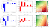Fig. 10. Change of particle pressure and fractions obtained in correspondence to the space-time coordinates explicitly marked in the left panel of Fig. 9 and corresponding to P/Psim = 0.94 (upper row) and P/Psim = 1.03 (lower row). The bar plots in blue (left) give the difference between the equilibrium pressure computed in post-processing and in the simulation, $\mathrm{\Delta }{P}_i=P_i-P_i^{ \text{sim}}$, where $i=\mathrm{tot},b,e^{-},e^{+},{\mu }^{-},{\mu }^{+},\gamma ,{\nu }_{\mathrm{e}},{\overline{\nu }}_{\mathrm{e}},{\nu }_{\mu },{\overline{\nu }}_{\mu },{\nu }_{\tau }$, and Ptot refers to the total pressure. The bar plots in red (centre) show the difference between the particle fractions computed in post-processing and the ones from the simulation, $\mathrm{\Delta }{Y}_i=Y_i-Y_i^{\text{sim}}$, where $i=n,p,e,\mu ,{\nu }_{\mathrm{e}},{\overline{\nu }}_{\mathrm{e}},{\nu }_{\mu },{\overline{\nu }}_{\mu }$, and e (μ) refers to the net electron (muon) fractions. The colour-coded plots (right) show Pb of BLh as a function of temperature and proton fraction for the same points. The density ρ is fixed to the value obtained in the simulation, that is, ρ = 4.3 × 1014 g cm−3 (upper row) and ρ = 1.55 ⋅ 1014 g cm−3 (lower row). The black star and the diamond mark are the values from the simulation (before post-processing) and at equilibrium (after post-processing), respectively.

for all the particle species at two representative points inside the simulations, explicitly marked in Fig. 9 and corresponding to P/P_sim ∼ 0.94 and P/P_sim ∼ 1.03, respectively. The drop in pressure was localised inside a hot spot at k_BT_sim ∼ 55 MeV, and it was mainly due to a decrease of baryonic pressure. Once muons were included in the microphysics, the system reached a new equilibrium characterised by a smaller neutron fraction; larger proton, electron, and muon fractions; and a smaller temperature (see also discussion in Sect. 4). The decrease in both the neutron fraction and of the temperature lowered the baryonic pressure, and the pressure provided by muons and trapped anti-neutrinos was not large enough to compensate. Accordingly, the total pressure also decreased. This effect is strongly correlated with the enhancement in the production of massive leptons and (anti-)neutrinos at high temperatures. An increase of pressure occurred at a lower initial temperature, k_BT_sim  ∼  15 MeV, and it was correlated with the inclusion of muons from the cold NSs. As shown in Fig. 2, including muons in cold neutrinoless β-equilibrium implies lowering the initial electron and neutron fraction in favour of the muon and proton fractions. Therefore, the pressure of the system increased because some relativistic particles (electrons) were replaced with non-relativistic particles (muons). An additional contribution came from the increase of the baryon pressure $\mathrm{\Delta }{P}_b=P_b-P_b^{\text{sim}}>0$, where P_b is computed in post-processing while $P_b^{\text{sim}}$ is read from the simulation outcome. In general, we would expect ΔP_b < 0 since the neutron fraction was reduced. However, we observed a small increase of temperature ΔT = 1.3 MeV, which was large enough to result in ΔP_b > 0, as shown in the colour-coded plot in the second row of Fig. 10. We note that the increase in temperature was expected because it is the only way the system could simultaneously reduce the number of neutrons and electrons, which are highly degenerate at k_BT_sim ∼ 15 MeV and at a fixed internal energy. Interestingly, adding new d.o.f. without supplementary repulsive forces did not simply result in a softening of the EOS, as we would have expected, because of the role played by the equilibrium temperature.

The causes of the changes in pressure in (DD2, 1.00) and (SFHo, 1.00) are the same as in (BLh, 1.00). From our analysis up to 15 ms after merger, we found that P/P_sim ranges from 0.94 to 1.05 for (DD2, 1.00) and from 0.93 to 1.04 for (SFHo, 1.00). As shown in Fig. 9, (DD2, 1.00) was subjected mostly to a pressure increase, while (SFHo, 1.00) exhibited a pressure increase in the region closer to the core and a pressure decrease in the outer shells. The amount of pressure decrease is comparable to the one found in Perego et al. (2019), while the pressure increase is a new prediction.

Pressure modifications correlate in a complex way with other thermodynamical variables, such as density, electron and muon fractions, temperature, and chemical potentials. However, a more important role is played by temperature. A close inspection of the distribution of P/P_sim in the $({\rho }_{\mathrm{sim}},T_{\mathrm{sim}},Y_{\mathrm{e}}^{\mathrm{sim}})$ space revealed that for all the EOSs, the pressure decrease was more frequent at larger T_sim. This is because electrons and muons are less degenerate, so the of conversion neutrons into protons is favoured and the baryonic pressure reduces to a greater extent. Regarding the pressure increase, it was frequent at smaller k_BT_sim < 20 MeV because of the dominant role played by the muons coming from the NSs in colder temperature regimes. We concluded that the remnant formed in (DD2, 1.00) exhibits mostly a pressure increase because its temperature is, on average, smaller compared to (BLh, 1.00) and (SFHo, 1.00).

We conclude this section by analysing how the pressure is modified in the case of an asymmetric binary mass ratio. If q = 1.43, then the ratio P/P_sim ranges in the interval 0.93 − 1.05, showing a pressure decrease compatible with the case where q = 1.00 but has a pressure increase that is significantly larger. This behaviour depends mostly on the difference between the electron fractions in the two simulations. In the case of q = 1.43, the regions with the highest P/P_sim also have a larger $Y_{\mathrm{e}}^{\mathrm{sim}}$ compared to q = 1.00 and as a consequence a larger ${\stackrel{\sim }{Y}}_{\mu }$ (see Fig. 2). Since the pressure increase is mainly driven by the muon fraction coming from the cold NSs, a larger ${\stackrel{\sim }{Y}}_{\mu }$ results in a larger P/P_sim. In Fig. 11, we show the comparison between the pressure ratios for q = 1.00 and q = 1.43 at approximately 7 ms after merger. We found that the spatial distribution of P/P_sim for q = 1.43 is quite asymmetric compared to q = 1.00 in the full-time domain of our analysis. In this case, the pressure decrease is localised in the core of the secondary NS, which is strongly heated by the shocks developing at the contact surface. The pressure increases in the cold external layers of the secondary NS, which are stripped away during the dynamical evolution without being significantly heated.

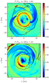Fig. 11. Pressure ratio P/Psim computed by post-processing (BLh, 1.00) (top) and (BLh, 1.43) (bottom) at 6.7 ms after merger. As in Fig. 1, the black lines mark the isodensity contours.

7. Discussion

Based on our results, in this section we speculate about the possible consequences for the evolution of the remnant and the emitted neutrinos. The fraction of muons is enhanced at high temperatures. Therefore, muons are expected to play a more important role in BNS mergers characterised by larger masses and in the case of soft EOSs producing more compact NSs. Such high temperatures develop mostly at the contact interface between the two fusing cores during the first milliseconds after a merger. In addition, CC reactions involving μ^±, ν_μ, and ${\overline{\nu }}_{\mu }$ provide a new source of opacity for muonic (anti-)neutrinos, as these reactions influence their diffusion. The neutrino surfaces of ${\overline{\nu }}_{\mu }$ and ν_μ are expected to split in a manner similar to ν_e and ${\overline{\nu }}_{\mathrm{e}}$ (Endrizzi et al. 2020), with the surface of ${\overline{\nu }}_{\mu }$ located at a larger rest mass density compared to ν_μ. Hence, the luminosity and the spectrum of the emitted ${\overline{\nu }}_{\mu }$ will deviate from that of ν_μ, with possible implications for the emitted spectrum and for the neutrino oscillations (see Fischer et al. 2020 for luminosity and spectra of ν_μ and ${\overline{\nu }}_{\mu }$ in CCSN). Furthermore, the formation of trapped degenerate gases of ν_e and ν_μ in the outer layers can favour the development of neutrino-bursts during the dynamical evolution, similar to the case of CCSN (Fischer et al. 2020), when dense, hot matter expands in the forming disc and becomes transparent. The change in pressure induced by muons and trapped neutrinos can change the time of the collapse of the remnant and affect the dynamical mass ejection. In particular, in (DD2, 1.00) and (SFHo, 1.00), we observed a diffuse pressure increase near the core (see discussion in Sect. 6), which can possibly postpone the collapse of the remnant. For (BLh, 1.00), the drop in pressure at high density induces a softening that could speed up the collapse of more massive binaries, while the larger pressure at smaller densities could affect the low-density dynamics, including the ejecta production, the disc formation, and the stability of the remnant produced in low mass BNS mergers. In Sect. 6, we established a correlation between P/P_sim and T_sim, pointing out that P/P_sim > 1 (P/P_sim < 1) when k_BT_sim is below (above) ∼20 MeV. This feature could induce positive feedback that amplifies pressure variations once muons and trapped neutrinos are included at the dynamical stage of the simulation. When the pressure decreases, the temperature of the more compressed system will increase, possibly triggering processes that lower the pressure even more. Nevertheless, when the pressure increases, the temperature of the expanded system will decrease, possibly favouring further pressure enhancement. However, feedback effects can be assessed only by including muons and trapped neutrinos in the dynamical evolution of the system. Moreover, the effect of pressure variations is, in general, non-trivial to predict. Indeed, pressure is one of the source terms in the Einstein equations and its significant increase could result in a faster collapse.

It is interesting to compare our results to the findings from CCSN simulations that include muons (Bollig et al. 2017; Fischer et al. 2020). Our estimate of Y_μ exceeds the muon fraction in the proximity of the core bounce by one order of magnitude (Fischer et al. 2020), while it is compatible with Y_μ in the late post-bounce phase (Bollig et al. 2017). This is because in CCSNe, matter density and temperature increase after the core bounce, while Y_e decreases, thus approaching the regime of our analysis. Since temperatures are significantly larger in BNS mergers than in CCSNe, thermal processes could contribute more significantly to the creation of μ^±, while they are negligible in CCSNe (Bollig et al. 2017; Guo et al. 2020; Fischer et al. 2020). However, the enhancement of the net muon fraction, Y_μ, with the temperature is in agreement with the results of Bollig et al. (2017), Fischer et al. (2020).

We note that while the inclusion of muons always implies a softening of the EOS in the post-bounce phase in CCSNe (Bollig et al. 2017; Fischer et al. 2020), in our case, the pressure can either increase or decrease with respect to the case where muons are neglected from the beginning. This difference is expected since in BNS mergers, the pressure increase obtained in our analysis is driven by the muons already present in the two cold NSs (see Sect. 6). Notably, muons are not present in stellar iron cores before a collapse.

Next, we relate our results to state-of-the-art BNS merger simulations that include trapped neutrinos either in post-processing (Perego et al. 2019) or through an M1 scheme (e.g. Foucart et al. 2016a; Radice et al. 2022; Zappa et al. 2023). The neutrino hierarchy resulting from our analysis is in disagreement with these works. In these previous papers, matter is dominated by ${\overline{\nu }}_{\mathrm{e}}$ and followed by heavy-lepton neutrinos and then ν_e, whereas we found that ${\overline{\nu }}_{\mu }$ are the most abundant, followed in order by ${\overline{\nu }}_{\mathrm{e}}$, ${\stackrel{(-)}{\nu }}_{\tau }$, ν_e, and ν_μ. According to Perego et al. (2019), the fluid pressure decreases after the inclusion of trapped neutrinos, but we show that it can also increase in some regions of the remnant. This is an indirect confirmation that the enhancement of pressure is mainly due to muons. Nonetheless, our estimate of the pressure decrease is compatible with the one computed in Perego et al. (2019).

8. Conclusions

In this paper, we evaluated the contribution of muons in the post-merger remnant formed during BNS mergers as well as their impact on the trapped neutrino component during the first milliseconds after the merger. In particular, we considered a sample of numerical relativity simulations targeted at GW170817 that were performed using three different nuclear EOSs (BLh, DD2, and SFHo). Based on the remnant conditions, we estimated the abundances and the properties of muons and trapped neutrinos in post-processing, assuming weak and thermal equilibrium for rest mass densities in excess of 10¹³ g cm⁻³. We found that a non-negligible amount of muons is present in the remnant, and they significantly alter the neutrino hierarchy, favouring the production of muon anti-neutrinos. Moreover, the new equilibrium conditions modify the pressure inside the remnant in a non-trivial way with respect to the case in which muons and trapped neutrinos are neglected.

More specifically, we found that a significant amount of muons is present at baryon densities ρ > 10¹³ g cm⁻³ with a fraction Y_μ⁻ ∼ 10⁻³ − 0.07 for the BLh EOS and Y_μ⁻ ∼ 10⁻³ − 0.05 for the DD2 and SFHo EOSs. The net fraction of muons is between 30% and 50–70% of the net electron fraction, with a maximum depending on the nuclear EOS. The bulk of muons comes from the two cold NSs, while a fraction corresponding to 10⁻³ − 10⁻² is created during the merger via conversion of neutrons into protons plus muons and thermal processes. Accordingly, muon production is enhanced in the high-density fusing cores and in the hot spots characterising the remnant structure during the first milliseconds after the merger.

The presence of muons modifies the flavour hierarchy of the trapped neutrino component. In the core, matter is dominated by anti-neutrinos, with ${\overline{\nu }}_{\mu }$ being the most abundant species. Immediately outside the core and in correspondence with the hot spots, gases of trapped neutrinos and anti-neutrinos coexist, but the ${\overline{\nu }}_{\mu }$ species still dominates, followed in order by ${\overline{\nu }}_{\mathrm{e}}$, ${\stackrel{(-)}{\nu }}_{\tau }$, ν_e, and ν_μ. In contrast, in the cold matter streams at ρ ∼ 10¹³ − 10¹⁴ g cm⁻³, anti-neutrinos are suppressed, while neutrinos dominate and the ν_μ species is the most abundant. Anti-neutrinos and neutrinos are degenerate in the core and in the cold matter streams, respectively. The level of degeneracy depends on the thermodynamical conditions of the remnant and on μ_n − μ_p. In particular, typical values of the degeneracy parameters of ${\overline{\nu }}_{\mathrm{e}}$ and ${\overline{\nu }}_{\mu }$ are ${\eta }_{{\overline{\nu }}_{\mathrm{e},\mu }}\sim 2-4$, with larger (smaller) values associated with larger (smaller) μ_n − μ_p. Therefore, the properties of trapped (anti-)neutrinos in BNS mergers have a non-trivial dependence on the properties of the EOS at densities well above n₀.

The presence of muons and trapped neutrinos affect the remnant pressure, whose value can decrease by 7% or increase by up to 5%, depending on the nuclear EOS, compared with the case in which they are neglected. The pressure drops mainly in the hot spots, where the processes driving muon production reduce the temperature and number of neutrons. The greater pressure mostly observed at low temperatures and high density is due to the muons coming from the cold NSs. This new result shows how adding a d.o.f. in the system microphysics does not always imply a decrease in pressure, as we could naively expect. Finally, we demonstrated that in asymmetric binaries, the pressure decrease is localised in the shocked core of the secondary NS, while the pressure increase is found in the cold outer layers of the secondary NS, which are stripped away by the primary NS.

Since the procedure to post-process the simulation data is not unique, in Appendix A we discuss the robustness of our results with respect to the arbitrary choices in our procedure. For example, we show that when neglecting muons inside the cold NSs before merger, the major results are the same as when the presence of muons in the inspiraling NSs is considered. The comparison with the first post-processing procedure emphasises that a significant muon contribution originates from the muons already present in the cold NSs.

Our work is nevertheless limited by the post-processing approach. To understand how muons really affect the merger and post-merger dynamics, it is necessary to implement a transport scheme that includes muons as an independent d.o.f.. Also, adding the rates of the reactions involved in muon production (see Sect. 2) would be important for estimating the effect of muons on the neutrino opacity and luminosity, as done in CCSN simulations (Guo et al. 2020; Fischer et al. 2020). Additionally, the role of pions coupling to muons and muonic (anti-)neutrinos should be considered while computing the mean free path of low energy ν_μ and ${\overline{\nu }}_{\mu }$ (Fore & Reddy 2020). We also highlight that in the description of NS matter, we have neglected the possible formation of hyperons (Oertel et al. 2012; Fortin et al. 2018) and/or that a deconfinement phase transition to quark matter may take place (Weissenborn et al. 2011; Klähn et al. 2013; Chatterjee & Vidaña 2016; Bombaci et al. 2016; Logoteta et al. 2019; Logoteta 2021). The inclusion of these additional d.o.f. will be the focus of future investigations.

This work shows, for the first time, that muons have a discernible impact on the trapped neutrino component and possibly on the thermodynamics and dynamics of BNS mergers. Our results emphasise the need of including muons in future simulation modelling of the post-merger remnant of BNS mergers.

Acknowledgments

The authors thank David Radice, Sebastiano Bernuzzi, Micaela Oertel, and Francesco Pederiva for useful discussions. They also thank the anonymous Referee for their valuable comments and suggestions. They acknowledge the INFN for the usage of computing and storage resources through the tullio cluster in Turin, and the Computational Relativity (CoRe) collaboration for providing access to the simulation data used in the work. MB and EL acknowledge financial support from MIUR (PRIN 2020 grant 2020KB33TP). MB acknowledges financial support from MIUR (PRIN 2017 grant 20179ZF5KS).

References

Appendix A: An alternative assumption on Y_l, μ

As discussed in Sect. 3.3, there is not a unique way to assign Y_l, μ, Y_l, e, and e_tot appearing on the left-hand side of Eq. (34) given the outcome of the simulations presented in Sect. 3.1. Therefore, in this Appendix, we consider a limiting case opposite to the one discussed in Sect. 3.3 as a different possible choice. In particular, we assume that muons are negligible in the initial conditions, that is, in the two cold NSs, and we impose Y_l, μ = 0. Then, we identify the simulation electron fraction, $Y_{\mathrm{e}}^{\mathrm{sim}}$, and energy density, e_sim, with Y_l, e and e_tot, respectively:

$$\begin{array}{c}\hfill Y_{l,e}=Y_{\mathrm{e}}^{\mathrm{sim}}{e}_{\mathrm{tot}}=e_{\mathrm{sim}},\end{array}$$(A.1)

(see from Eq. (30) to Eq. (33)). This choice, despite being inconsistent with what we expect, has the advantage of being fully coherent with the simulation assumptions, and it provides an easier initialisation of our post-processing calculation. In the following paragraphs, we discuss the results obtained with this choice, and we compare them with the ones discussed in the previous sections. From this point on, we refer to this particular choice as Y_l, μ = 0 and to the one discussed in Sect. 3.3 as $Y_{l,\mu }={\stackrel{\sim }{Y}}_{\mu }$.

A.1. The fraction of muons

If Y_l, μ = 0, all the muons in the final state are produced during the merger. For all the simulations in Table 1, the equilibrium muon fraction at density ρ > 10¹⁴ g cm⁻³ is Y_μ⁻ ∼ 10⁻³ − 3 × 10⁻². At a lower density, ρ ∼ 10¹³ − 10¹⁴ g cm⁻³, the muon fraction is Y_μ⁻ ∼ 10⁻³ if T_sim ≳ 10 MeV; otherwise, muons are not present. We note that the amount of muons produced only during the merger is slightly smaller when $Y_{l,\mu }={\stackrel{\sim }{Y}}_{\mu }$ (see Sect. 4) because of the Pauli blocking coming from the muons already present in the cold NSs.

For all the simulations, Y_μ/Y_e ∼ 0.3 − 0.4, but the maximum Y_μ/Y_e is larger for DD2 and SFHo than for BLh because the latter exhibits a larger Y_e (see also Fig. 2). The creation of muons is enhanced in correspondence to the hot spots for all the EOSs. In the case of (BLh, 1.00), muon production also increases in the density region ρ > 10¹⁵ g cm⁻³. This effect depends on the significantly larger electron fraction obtained with the BLh EOS since the more degenerate electrons block the conversion of neutrons into protons plus electrons, favouring instead the conversion into protons plus muons.

A.2. The trapping of neutrinos

The initial assumption on Y_l, μ does not significantly affect the behaviour of electron (anti-)neutrinos, but it does imply discernible consequences on the muon neutrinos. If Y_l, μ = 0, muon neutrinos appear only in correspondence to the hot spots and the warm matter streams, with a maximum fraction Y_νμ ∼ 0.01. All ν_μ are produced together with ${\overline{\nu }}_{\mu }$ since there is not an initial muon fraction that can be converted into ν_μ. In contrast, the amount of ${\overline{\nu }}_{\mu }$ at equilibrium is strongly enhanced to guarantee the conservation of Y_l, μ. Therefore, $Y_{{\overline{\nu }}_{\mu }}\approx Y_{{\mu }^{-}}$ for all the simulations considered, and ${\overline{\nu }}_{\mu }$ constitute the most abundant species amongst all flavour (anti-)neutrinos in the regions that are not dominated by thermal production.

The differences in the equilibrium fractions of neutrinos depending on the chosen Y_l, μ reflect the differences in the degeneracy parameters. For all the simulations η_νμ ≤ 0 and the production of ν_μ, only thermal and trapped degenerate ν_μ are suppressed. In addition, the gases of ${\overline{\nu }}_{\mathrm{e}}$ and ${\overline{\nu }}_{\mu }$ trapped in the remnant core are more degenerate when Y_l, μ = 0 compared to when $Y_{l,\mu }={\stackrel{\sim }{Y}}_{\mu }$. This follows in part from the enhanced production of ${\overline{\nu }}_{\mu }$ when Y_l, μ = 0, but it also depends on the equilibrium temperature T, which is systematically larger when $Y_{l,\mu }={\stackrel{\sim }{Y}}_{\mu }$. Actually, in the latter case, the system lowers the fraction of electrons and neutrons to take into account the fraction of muons from the cold NSs, which practically means reducing the system degeneracy by increasing the temperature (see the discussions in Sect. 3.3 and Sect. 6).

We stress that the presence of a trapped degenerate component of ${\overline{\nu }}_{\mathrm{e}}$ and ${\overline{\nu }}_{\mu }$ in the core and of ν_e in the outer layers of the remnant is a robust prediction independent of the initial assumption on Y_l, μ. Instead, the presence of a degenerate gas of ν_μ in the cold matter streams depends on the initial choice of Y_l, μ.

A.3. The changes in pressure

In conclusion, we analysed the ratio P/P_sim where P is computed in post-processing under the assumption Y_l, μ = 0. In this case, we did not observe a significant pressure increase after muons were introduced (i.e. P/P_sim > 1) for any of the simulations in Table 1. This result is expected since, within this assumption, we neglected the muons from the cold NSs, which are indeed responsible for the pressure increase when $Y_{l,\mu }={\stackrel{\sim }{Y}}_{\mu }$, as discussed in Sect. 6. In fact, the amount and the spatial distribution of the pressure decrease are common to all the simulations irrespective of the initial assumption on Y_l, μ. In particular, the pressure decrease is still favoured in correspondence to the hot spots because, in these regions, the final equilibrium fractions of muons and (anti-)neutrinos are comparable for the two choices of Y_l, μ.

All Tables

All Figures

Fig. 1. Outcome of the numerical simulation (BLh, 1.00) at 4.6 ms after merger. The left, central, and right panels show the rest mass density, the temperature, and the electron fraction on the equatorial plane, respectively. The black lines mark isodensity contours corresponding to 1012 g cm−3 (solid line), 1013 g cm−3 (dashed line), 1014 g cm−3 (dashed-dotted line), and 1015 g cm−3 (dotted line).

In the text

Fig. 2. Particle fractions computed at T = 0 in neutrinoless β-equilibrium for three different EOS: BLh (left), DD2 (centre), and SFHo (right). Black lines show the electron fraction computed in two different cases: equilibrium with muons (solid lines) or without muons (dashed lines). The green line corresponds to the fraction of protons at equilibrium with muons, while the red line corresponds to the muon fraction. We note that when muons are not included, the proton fraction coincides with the electron one (dashed black line).

In the text

Fig. 3. Particle fractions and chemical potential in the muon flavour sector computed by post-processing the simulation (BLh, 1.00) at 4.6 ms after merger. In the upper panels, we show the fraction of μ− (left), the fraction of μ+ (centre), and the difference between the muon fraction and the one inherited from the cold NSs, that is, $Y_{{\mu }^{-}}-{\stackrel{\sim }{Y}}_{\mu }$ (right). In the lower panels, we show the fraction of νμ (left), the fraction of ${\overline{\nu }}_{\mu }$ (centre), and the muon chemical potential (rest mass subtracted) (right). As in Fig. 1, the black lines mark isodensity contours.

In the text

	Fig. 4. Ratio of the net muon fraction over the net electron fraction, Yμ/Ye, on the equatorial plane obtained by post-processing simulations (BLh, 1.00) (upper left), (BLh, 1.43) (upper right), (DD2, 1.00) (lower left), and (SFHo, 1.00) (lower right) at 5 − 6 ms after merger. As in Fig. 1, the black lines mark isodensity contours.
In the text

Fig. 5. Fractions of νe, ${\overline{\nu }}_{\mathrm{e}}$, ντ, and chemical potentials of electrons, protons, and neutrons computed in post-processing for (BLh, 1.00) at 4.6 ms after merger. In the upper panels, we show the fraction of νe (left), the fraction of ${\overline{\nu }}_{\mathrm{e}}$ (centre), and the fraction of ντ (right). In the lower panels, we show the electron chemical potential (rest mass subtracted) μe − me (left), the proton chemical potential (rest mass subtracted) μp − mp (centre), and the neutron chemical potential (rest mass subtracted) μn − mn (right). We note that the colour bar scales are different for the various chemical potentials. As in Fig. 1, the black lines mark the isodensity contours.

In the text

Fig. 6. Proton and neutron chemical potentials (rest mass subtracted) of BLh in the density-temperature plane at fixed Yp = 0.08. The proton fraction Yp = 0.08 is the equilibrium proton fraction at 4.6 ms after merger around the point x = 0.64 km, y = 12.76 km, z = 0 km, where ρ ∼ 5 × 1013 g cm−3, Tsim ∼ 10 MeV, and neutrinos dominate, while anti-neutrinos are suppressed (see also Figs. 1, 3 and 5). We notice that the colour bars are scaled differently.

In the text

	Fig. 7. Degeneracy parameter of νe (first row) and νμ (lower row) on the equatorial plane obtained by post-processing the simulation (BLh, 1.00). Three different time slices are shown corresponding from left to right to 4.6 ms, 6.7 ms, and 11.8 ms after merger. As in Fig. 1, the black lines mark the isodensity contours as in Fig. 1.
In the text

	Fig. 8. Mean energy Eν of trapped neutrinos on the equatorial plane computed by post-processing simulation (BLh, 1.00) at 4.6 ms after merger. As in Fig. 1., the black lines mark isodensity contours.
In the text

	Fig. 9. Pressure ratio P/Psim for (BLh, 1.00) (left), (DD2, 1.00) (centre), and (SFHo, 1.00) (right) where P is obtained in post-processing, while Psim is the simulation pressure. For (BLh, 1.00), we explicitly mark the maximum P/Psim ∼ 1.03 (white circle) and the minimum P/Psim ∼ 0.94 (white cross) at ρ > 1014 g cm−3. As in Fig. 1., the black lines mark isodensity contours.
In the text

Fig. 10. Change of particle pressure and fractions obtained in correspondence to the space-time coordinates explicitly marked in the left panel of Fig. 9 and corresponding to P/Psim = 0.94 (upper row) and P/Psim = 1.03 (lower row). The bar plots in blue (left) give the difference between the equilibrium pressure computed in post-processing and in the simulation, $\mathrm{\Delta }{P}_i=P_i-P_i^{ \text{sim}}$, where $i=\mathrm{tot},b,e^{-},e^{+},{\mu }^{-},{\mu }^{+},\gamma ,{\nu }_{\mathrm{e}},{\overline{\nu }}_{\mathrm{e}},{\nu }_{\mu },{\overline{\nu }}_{\mu },{\nu }_{\tau }$, and Ptot refers to the total pressure. The bar plots in red (centre) show the difference between the particle fractions computed in post-processing and the ones from the simulation, $\mathrm{\Delta }{Y}_i=Y_i-Y_i^{\text{sim}}$, where $i=n,p,e,\mu ,{\nu }_{\mathrm{e}},{\overline{\nu }}_{\mathrm{e}},{\nu }_{\mu },{\overline{\nu }}_{\mu }$, and e (μ) refers to the net electron (muon) fractions. The colour-coded plots (right) show Pb of BLh as a function of temperature and proton fraction for the same points. The density ρ is fixed to the value obtained in the simulation, that is, ρ = 4.3 × 1014 g cm−3 (upper row) and ρ = 1.55 ⋅ 1014 g cm−3 (lower row). The black star and the diamond mark are the values from the simulation (before post-processing) and at equilibrium (after post-processing), respectively.

In the text

References

- Abbott, B. P., Abbott, R., Abbott, T. D., et al. 2017a, Phys. Rev. Lett., 119, 161101 [Google Scholar]
- Abbott, B. P., Abbott, R., Abbott, T. D., et al. 2017b, ApJ, 848, L12 [Google Scholar]
- Abbott, B. P., Abbott, R., Abbott, T. D., et al. 2018, Phys. Rev. Lett., 121, 161101 [Google Scholar]
- Abbott, B. P., Abbott, R., Abbott, T. D., et al. 2019, Phys. Rev. X, 9, 011001 [Google Scholar]
- Abbott, B. P., Abbott, R., Abbott, T. D., et al. 2020, Liv. Rev. Relativ., 23, 3 [NASA ADS] [CrossRef] [Google Scholar]
- Alford, M., Harutyunyan, A., & Sedrakian, A. 2021, Phys. Rev. D, 104, 103027 [NASA ADS] [CrossRef] [Google Scholar]
- Alford, M. G., & Good, G. 2010, Phys. Rev. C, 82, 055805 [NASA ADS] [CrossRef] [Google Scholar]
- Antoniadis, J., Freire, P. C. C., Wex, N., et al. 2013, Science, 340, 448 [Google Scholar]
- Bauswein, A., Janka, H. T., Hebeler, K., & Schwenk, A. 2012, Phys. Rev. D, 86, 063001 [Google Scholar]
- Bauswein, A., Just, O., Janka, H.-T., & Stergioulas, N. 2017, ApJ, 850, L34 [Google Scholar]
- Bernuzzi, S. 2020, General Relativ. Gravitation, 52, 108 [CrossRef] [Google Scholar]
- Bernuzzi, S., Radice, D., Ott, C. D., et al. 2016, Phys. Rev. D, 94, 024023 [Google Scholar]
- Bernuzzi, S., Breschi, M., Daszuta, B., et al. 2020, MNRAS, 497, 1488 [Google Scholar]
- Bludman, S. A., & van Riper, K. A. 1977, ApJ, 212, 859 [NASA ADS] [CrossRef] [Google Scholar]
- Bollig, R., DeRocco, W., Graham, P. W., & Janka, H.-T. 2020, Phys. Rev. Lett., 125, 051104 [NASA ADS] [CrossRef] [Google Scholar]
- Bollig, R., Janka, H. T., Lohs, A., et al. 2017, Phys. Rev. Lett., 119, 242702 [NASA ADS] [CrossRef] [Google Scholar]
- Bombaci, I., & Logoteta, D. 2018, A&A, 609, A128 [EDP Sciences] [Google Scholar]
- Bombaci, I., Logoteta, D., Vidaña, I., & Providência, C. 2016, Eur. Phys. J. A, 52, 58 [NASA ADS] [CrossRef] [Google Scholar]
- Breschi, M., Gamba, R., & Bernuzzi, S. 2021, Phys. Rev. D, 104, 042001 [NASA ADS] [CrossRef] [Google Scholar]
- Breschi, M., Bernuzzi, S., Godzieba, D., Perego, A., & Radice, D. 2022, Phys. Rev. Lett., 128, 161102 [NASA ADS] [CrossRef] [Google Scholar]
- Cameron, A. G. W. 1970, ARA&A, 8, 179 [NASA ADS] [CrossRef] [Google Scholar]
- Chatterjee, D., & Vidaña, I. 2016, Eur. Phys. J. A, 52, 29 [NASA ADS] [CrossRef] [Google Scholar]
- Cohen, J. M., Langer, W. D., Rosen, L. C., & Cameron, A. G. W. 1970, Ap&SS, 6, 228 [NASA ADS] [CrossRef] [Google Scholar]
- Colombo, A., Salafia, O. S., Gabrielli, F., et al. 2022, ApJ, 937, 79 [NASA ADS] [CrossRef] [Google Scholar]
- Cooperstein, J. 1988, Phys. Rept., 163, 95 [NASA ADS] [CrossRef] [Google Scholar]
- Cusinato, M., Guercilena, F. M., Perego, A., et al. 2022, EPJA, 58, 99 [NASA ADS] [CrossRef] [EDP Sciences] [Google Scholar]
- Damour, T., Nagar, A., & Villain, L. 2012, Phys. Rev. D, 85, 123007 [NASA ADS] [CrossRef] [Google Scholar]
- Danielewicz, P., & Lee, J. 2014, Nucl. Phys. A, 922, 1 [NASA ADS] [CrossRef] [Google Scholar]
- De, S., Finstad, D., Lattimer, J. M., et al. 2018, Phys. Rev. Lett., 121, 091102; Erratum: 121, 259902 [Google Scholar]
- Drischler, C., Hebeler, K., & Schwenk, A. 2019, Phys. Rev. Lett., 122, 042501 [Google Scholar]
- Endrizzi, A., Perego, A., Fabbri, F. M., et al. 2020, Eur. Phys. J. A, 56, 15 [EDP Sciences] [Google Scholar]
- Evans, M., Adhikari, R. X., Afle, C., et al. 2021, ApJ, submitted [arXiv:2109.09882] [Google Scholar]
- Favata, M. 2014, Phys. Rev. Lett., 112, 101101 [NASA ADS] [CrossRef] [Google Scholar]
- Fischer, T., Guo, G., Martínez-Pinedo, G., Liebendörfer, M., & Mezzacappa, A. 2020, Phys. Rev. D, 102, 123001 [NASA ADS] [CrossRef] [Google Scholar]
- Fore, B., & Reddy, S. 2020, Phys. Rev. C, 101, 035809 [NASA ADS] [CrossRef] [Google Scholar]
- Fortin, M., Oertel, M., & Providência, C. 2018, PASA, 35, e044 [NASA ADS] [CrossRef] [Google Scholar]
- Foucart, F., Haas, R., Duez, M. D., et al. 2016a, Phys. Rev. D, 93, 044019 [NASA ADS] [CrossRef] [Google Scholar]
- Foucart, F., O’Connor, E., Roberts, L., et al. 2016b, Phys. Rev. D, 94, 123016 [NASA ADS] [CrossRef] [Google Scholar]
- Glendenning, N. K. 1997, Compact stars. Nuclear Physics, Particle Physics, and General Relativity [Google Scholar]
- Grimm, S., & Harms, J. 2020, Phys. Rev. D, 102, 022007 [NASA ADS] [CrossRef] [Google Scholar]
- Guo, G., Martínez-Pinedo, G., Lohs, A., & Fischer, T. 2020, Phys. Rev. D, 102, 023037 [NASA ADS] [CrossRef] [Google Scholar]
- Haensel, P., Levenfish, K. P., & Yakovlev, D. G. 2000, A&A, 357, 1157 [NASA ADS] [Google Scholar]
- Haensel, P., Levenfish, K. P., & Yakovlev, D. G. 2001, A&A, 372, 130 [NASA ADS] [CrossRef] [EDP Sciences] [Google Scholar]
- Haft, M., Raffelt, G., & Weiss, A. 1994, ApJ, 425, 222; Erratum: 1995, 438, 1017 [NASA ADS] [CrossRef] [Google Scholar]
- Hammond, P., Hawke, I., & Andersson, N. 2022, ApJ, submitted [arXiv:2205.11377] [Google Scholar]
- Hannestad, S., & Raffelt, G. 1998, ApJ, 507, 339 [NASA ADS] [CrossRef] [Google Scholar]
- Hempel, M., & Schaffner-Bielich, J. 2010, Nucl. Phys. A, 837, 210 [Google Scholar]
- Hinderer, T. 2008, ApJ, 677, 1216 [NASA ADS] [CrossRef] [Google Scholar]
- Hix, W. R., & Thielemann, F.-K. 1999, ApJ, 511, 862 [NASA ADS] [CrossRef] [Google Scholar]
- Iacovelli, F., Mancarella, M., Foffa, S., & Maggiore, M. 2022, ApJ, 941, 208 [NASA ADS] [CrossRef] [Google Scholar]
- Kaplan, J. D., Ott, C. D., O’Connor, E. P., et al. 2014, ApJ, 790, 19 [NASA ADS] [CrossRef] [Google Scholar]
- Klähn, T., Łastowiecki, R., & Blaschke, D. B. 2013, Phys. Rev. D, 88, 085001 [CrossRef] [Google Scholar]
- Lattimer, J. M., & Steiner, A. W. 2014, ApJ, 784, 123 [Google Scholar]
- Leinson, L. B. 2002, Nucl. Phys. A, 707, 543 [NASA ADS] [CrossRef] [Google Scholar]
- Logoteta, D. 2021, Universe, 7, 408 [NASA ADS] [CrossRef] [Google Scholar]
- Logoteta, D., Vidana, I., & Bombaci, I. 2019, Eur. Phys. J. A, 55, 207 [CrossRef] [Google Scholar]
- Logoteta, D., Perego, A., & Bombaci, I. 2021, A&A, 646, A55 [NASA ADS] [CrossRef] [EDP Sciences] [Google Scholar]
- Maggiore, M., Van Den Broeck, C., Bartolo, N., et al. 2020, J. Cosmol. Astropart. Phys., 2020, 050 [CrossRef] [Google Scholar]
- Margalit, B., & Metzger, B. D. 2017, ApJ, 850, L19 [Google Scholar]
- Miller, M. C., Lamb, F. K., Dittmann, A. J., et al. 2019, ApJ, 887, L24 [Google Scholar]
- Miller, M. C., Lamb, F. K., Dittmann, A. J., et al. 2021, ApJ, 918, L28 [NASA ADS] [CrossRef] [Google Scholar]
- Most, E. R., Papenfort, L. J., Dexheimer, V., et al. 2019, Phys. Rev. Lett., 122, 061101 [NASA ADS] [CrossRef] [Google Scholar]
- Nedora, V., Bernuzzi, S., Radice, D., et al. 2019, ApJ, 886, L30 [NASA ADS] [CrossRef] [Google Scholar]
- Nedora, V., Bernuzzi, S., Radice, D., et al. 2021, ApJ, 906, 98 [NASA ADS] [CrossRef] [Google Scholar]
- Oertel, M., Fantina, A. F., & Novak, J. 2012, Phys. Rev. C, 85, 055806 [NASA ADS] [CrossRef] [Google Scholar]
- Oertel, M., Hempel, M., Klähn, T., & Typel, S. 2017, Rev. Modern Phys., 89, 015007 [NASA ADS] [CrossRef] [Google Scholar]
- Patricelli, B., Bernardini, M. G., Mapelli, M., et al. 2022, MNRAS, 513, 4159 [NASA ADS] [CrossRef] [Google Scholar]
- Perego, A., Bernuzzi, S., & Radice, D. 2019, Eur. Phys. J. A, 55, 124 [EDP Sciences] [Google Scholar]
- Perego, A., Logoteta, D., Radice, D., et al. 2022, Phys. Rev. Lett., 129, 032701 [NASA ADS] [CrossRef] [Google Scholar]
- Potekhin, A. Y., Pons, J. A., & Page, D. 2015, Space Sci. Rev., 191, 239 [Google Scholar]
- Prakash, M., Bombaci, I., Prakash, M., et al. 1997, Phys. Rep., 280, 1 [Google Scholar]
- Punturo, M., Abernathy, M., Acernese, F., et al. 2010, CQG, 27, 194002 [NASA ADS] [CrossRef] [Google Scholar]
- Raaijmakers, G., Greif, S. K., Hebeler, K., et al. 2021, ApJ, 918, L29 [NASA ADS] [CrossRef] [Google Scholar]
- Radice, D., Galeazzi, F., Lippuner, J., et al. 2016, MNRAS, 460, 3255 [NASA ADS] [CrossRef] [Google Scholar]
- Radice, D., Perego, A., Hotokezaka, K., et al. 2018a, ApJ, 869, 130 [Google Scholar]
- Radice, D., Perego, A., Zappa, F., & Bernuzzi, S. 2018b, ApJ, 852, L29 [NASA ADS] [CrossRef] [Google Scholar]
- Radice, D., Bernuzzi, S., & Perego, A. 2020, Ann. Rev. Nucl. Part. Sci., 70, 95 [NASA ADS] [CrossRef] [Google Scholar]
- Radice, D., Bernuzzi, S., Perego, A., & Haas, R. 2022, MNRAS, 512, 1499 [NASA ADS] [CrossRef] [Google Scholar]
- Richers, S. A., McLaughlin, G. C., Kneller, J. P., & Vlasenko, A. 2019, Phys. Rev. D, 99, 123014 [NASA ADS] [CrossRef] [Google Scholar]
- Riley, T. E., et al. 2019, ApJ, 887, L21 [CrossRef] [Google Scholar]
- Ronchini, S., Branchesi, M., Oganesyan, G., et al. 2022, A&A, 665, A97 [NASA ADS] [CrossRef] [EDP Sciences] [Google Scholar]
- Rosswog, S., & Liebendoerfer, M. 2003, MNRAS, 342, 673 [NASA ADS] [CrossRef] [Google Scholar]
- Ruffert, M., & Janka, H. T. 1998, A&A, 338, 535 [NASA ADS] [Google Scholar]
- Ruffert, M., Janka, H. T., & Schaefer, G. 1996, A&A, 311, 532 [NASA ADS] [Google Scholar]
- Sekiguchi, Y., Kiuchi, K., Kyutoku, K., & Shibata, M. 2011a, Phys. Rev. Lett., 107, 211101 [NASA ADS] [CrossRef] [Google Scholar]
- Sekiguchi, Y., Kiuchi, K., Kyutoku, K., & Shibata, M. 2011b, Phys. Rev. Lett., 107, 051102 [NASA ADS] [CrossRef] [Google Scholar]
- Sekiguchi, Y., Kiuchi, K., Kyutoku, K., Shibata, M., & Taniguchi, K. 2016, Phys. Rev. D, 93, 124046 [NASA ADS] [CrossRef] [Google Scholar]
- Shapiro, S. L., & Teukolsky, S. A. 1983, Black Holes, White Dwarfs, and Neutron Stars : the Physics of Compact Objects [Google Scholar]
- Shlomo, S., Kolomietz, V. M., & Colò, G. 2006, Eur. Phys. J. A, 30, 23 [NASA ADS] [CrossRef] [Google Scholar]
- Steiner, A. W., Prakash, M., Lattimer, J. M., & Ellis, P. J. 2005, Phys. Rep., 411, 325 [NASA ADS] [CrossRef] [Google Scholar]
- Steiner, A. W., Hempel, M., & Fischer, T. 2013, ApJ, 774, 17 [NASA ADS] [CrossRef] [Google Scholar]
- Takami, K., Rezzolla, L., & Baiotti, L. 2014, Phys. Rev. Lett., 113, 091104 [NASA ADS] [CrossRef] [Google Scholar]
- Timmes, F. X., & Arnett, D. 1999, ApJS, 125, 277 [Google Scholar]
- Typel, S., Röpke, G., Klähn, T., Blaschke, D., & Wolter, H. H. 2010, Phys. Rev. C, 81, 015803 [NASA ADS] [CrossRef] [Google Scholar]
- Weih, L. R., Hanauske, M., & Rezzolla, L. 2020, Phys. Rev. Lett., 124, 171103 [NASA ADS] [CrossRef] [Google Scholar]
- Weissenborn, S., Sagert, I., Pagliara, G., Hempel, M., & Schaffner-Bielich, J. 2011, ApJ, 740, L14 [NASA ADS] [CrossRef] [Google Scholar]
- Yakovlev, D. G., & Pethick, C. J. 2004, ARA&A, 42, 169 [NASA ADS] [CrossRef] [Google Scholar]
- Zappa, F., Bernuzzi, S., Radice, D., Perego, A., & Dietrich, T. 2018, Phys. Rev. Lett., 120, 111101 [NASA ADS] [CrossRef] [Google Scholar]
- Zappa, F., Bernuzzi, S., Radice, D., & Perego, A. 2023, MNRAS, 520, 1481 [Google Scholar]