| Issue |
A&A
Volume 666, October 2022
|
|
|---|---|---|
| Article Number | A174 | |
| Number of page(s) | 16 | |
| Section | Astrophysical processes | |
| DOI | https://doi.org/10.1051/0004-6361/202243260 | |
| Published online | 24 October 2022 | |
Constraints on the merging binary neutron star mass distribution and equation of state based on the incidence of jets in the population⋆
1
Università degli Studi di Milano-Bicocca, Dip. di Fisica “G. Occhialini”, piazza della Scienza 3, 20126 Milano (MI), Italy
e-mail: This email address is being protected from spambots. You need JavaScript enabled to view it.
2
INFN – Sezione di Milano-Bicocca, piazza della Scienza 2, 20126 Milano (MI), Italy
3
INAF – Osservatorio Astronomico di Brera, Via E. Bianchi 46, 23807 Merate (LC), Italy
4
Scuola Internazionale Superiore di Studi Avanzati (SISSA), Via Bonomea 265, 34136 Trieste (TS), Italy
5
Monash Centre for Astrophysics, School of Physics and Astronomy, Monash University, Clayton, Victoria 3800, Australia
6
ARC Center of Excellence for Gravitational Wave Discovery – OzGrav, Hawthorn, Australia
7
Institute of Gravitational Wave Astronomy and School of Physics and Astronomy, University of Birmingham, Birmingham B15 2TT, UK
Received:
3
February
2022
Accepted:
1
August
2022
Abstract
A relativistic jet has been produced in the single well-localised binary neutron star (BNS) merger detected to date in gravitational waves (GWs), and the local rates of BNS mergers and short gamma-ray bursts are of the same order of magnitude. This suggests that jet formation is not a rare outcome for BNS mergers, and we show that this intuition can be turned into a quantitative constraint: at least about one-third of GW-detected BNS mergers and at least about one-fifth of all BNS mergers should produce a successful jet (90% credible level). Whether a jet is launched depends on the properties of the merger remnant and of the surrounding accretion disc, which in turn are a function of the progenitor binary masses and equation of state (EoS). The incidence of jets in the population therefore carries information about the binary component mass distribution and EoS. Under the assumption that a jet can only be produced by a black hole remnant surrounded by a non-negligible accretion disc, we show how the jet incidence can be used to place a joint constraint on the space of BNS component mass distributions and EoS. The result points to a broad mass distribution, with particularly strong support for masses in the 1.3 − 1.6 M⊙ range. The constraints on the EoS are shallow, but we show how they will tighten as the knowledge on the jet incidence improves. We also discuss how to extend the method to include future BNS mergers, with possibly uncertain jet associations.
Key words: gravitational waves / gamma-ray burst: general / stars: neutron / pulsars: general / stars: luminosity function, mass function / relativistic processes
The source code of the manuscript and that used to produce all figures is publicly available at https://github.com/omsharansalafia/bns_jet_incidence_public
© O. S. Salafia et al. 2022
 Open Access article, published by EDP Sciences, under the terms of the Creative Commons Attribution License (https://creativecommons.org/licenses/by/4.0), which permits unrestricted use, distribution, and reproduction in any medium, provided the original work is properly cited.
This article is published in open access under the Subscribe-to-Open model.
1. Introduction
Binary neutron star (BNS) mergers have long been considered (Eichler et al. 1989) as promising candidate progenitors of at least some gamma-ray bursts (GRBs). Evidence accumulated through the years has pointed to the two observational GRB classes (‘long’ and ‘short’, Kouveliotou et al. 1993) being physically linked to two different progenitors, with collapsars (Woosley 1993) being the progenitors of long GRBs, and BNS mergers (and possibly also neutron star – black hole mergers, Mochkovitch et al. 1993) being those of short GRBs (SGRBs, Berger 2014; D’Avanzo 2015). The confirmation of the collapsar progenitor scenario for long GRBs came with the association of GRB980425 with supernova SN1998bw (Galama et al. 1998). The clear evidence (Abbott et al. 2017; Mooley et al. 2018; Ghirlanda et al. 2019) in support of the presence of a relativistic jet in association with the GW170817 BNS merger detected by the Advanced Laser Interferometer Gravitational-wave Observatory (aLIGO, Aasi et al. 2015) and Virgo (Acernese et al. 2014) network – observed under a relatively large viewing angle with respect to its axis – and the fact that the inferred characteristics of such a jet indicate (e.g. Salafia et al. 2019) that an on-axis observer would have observed an emission consistent with previously known SGRBs have provided long-awaited compelling evidence in support of the BNS-SGRB progenitor scenario. Still, the question of whether all BNS mergers produce a jet (and whether other progenitors contribute a significant fraction of SGRBs) remains open. The answer to this question encodes information about the conditions that lead to the launch of a jet and to its successful propagation up to the location where the observable emission is produced.
The conditions for the launch of a relativistic jet in the immediate aftermath of a BNS merger are set by the jet-launching mechanism, which is not entirely settled: while the Blandford & Znajek (1977) mechanism – which involves the extraction of energy from a spinning black hole by magnetic fields supported by an accretion disc – seems to be the most favoured one, several authors (e.g. Dai & Lu 1998; Zhang & Mészáros 2001; Metzger et al. 2008; Dall’Osso et al. 2011; Bernardini et al. 2012a,b, 2013; Rowlinson et al. 2013; Gompertz et al. 2013; Stratta et al. 2018; Strang & Melatos 2019; Sarin et al. 2020) invoked a rapidly spinning, highly magnetised neutron star (a proto-magnetar) to explain some observational features such as the so-called plateaux (Nousek et al. 2006) in early X-ray afterglows and the detection of ‘extended emission’ (Norris & Bonnell 2006) in gamma rays beyond the usual short-duration prompt emission. On the other hand, many models of the early X-ray afterglow and extended emission do not require a proto-magnetar (e.g. Rees & Mészáros 1998; Zhang et al. 2006; Genet et al. 2007; Yamazaki 2009; Leventis et al. 2014; Duffell & MacFadyen 2015; Beniamini et al. 2020; Oganesyan et al. 2020; Ascenzi et al. 2020; Barkov et al. 2021; Duque et al. 2022), and the production of a successful jet by such a compact object, while possible (Usov 1992; Thompson 1994; Thompson et al. 2004; Metzger et al. 2011; Mösta et al. 2020), is theoretically disfavoured (e.g. Ciolfi 2020, see also Sect. 3.1).
Whether a BNS merger satisfies the jet-launching conditions, regardless of what they are, depends on the progenitor system parameters and on the equation of state (EoS) of neutron star matter (Fryer et al. 2015; Piro et al. 2017). Indeed, despite their complexity, the merger dynamics are mostly deterministic, so that the properties of the post-merger remnant and any accretion disc are directly linked to the progenitor binary masses and, in principle, spins and magnetic fields. Except for extreme cases, however, are pre-merger neutron star spins and magnetic fields thought to have a limited impact (e.g. East et al. 2019; Dudi et al. 2022; Papenfort et al. 2022 for spins; e.g. Giacomazzo et al. 2009; Lira et al. 2022 for magnetic fields). Moreover, the magnetic field in the merger remnant and accretion disc is thought to undergo amplification due to Kelvin-Helmholtz instabilities and dynamo processes (e.g. Kiuchi et al. 2014, 2015; Palenzuela et al. 2022), leading to the loss of memory about the initial magnetisation. Therefore, the fraction of jet-launching systems in the BNS merger population is largely determined by the distribution of the progenitor binary masses and by the properties of neutron star matter, that is, by the (not yet well-known) EoS of matter beyond the nuclear saturation density. The incidence of jets in the population therefore carries information about both binary stellar evolution and nuclear physics, which can be investigated especially through multi-messenger observations of these sources.
In principle, a relativistic jet may be launched, but not be able to propagate through the cloud of merger ejecta and break out of it, and some authors have suggested (e.g. Moharana & Piran 2017) that this is a frequent outcome. On the other hand, the expected properties of BNS merger ejecta and those of SGRB jets (also in light of GW170817) suggest that the vast majority of jets are successful in breaking out (Duffell et al. 2018; Beniamini et al. 2019; Salafia et al. 2020). In this article, we therefore consider systems that satisfy our ‘jet-launching conditions’ to always lead to a successful jet breakout.
In what follows, we derive the posterior probability distributions on the jet incidence, that is to say the fraction of systems that launch a jet in BNS mergers based on the presence of a jet in GW170817 (Sect. 2.1) and on the comparison of local rate densities of SGRBs and BNS mergers (Sect. 2.2). We then describe a framework to model the jet incidence under the physically motivated assumption that launching a jet in the aftermath of the merger requires the collapse of the remnant to a black hole on a short timescale and the presence of a non-negligible accretion disc (Sect. 3). Within this framework, we show that knowledge of the jet incidence can be used to constrain the BNS mass distribution and the EoS (Sect. 4.1). We show (Sect. 4.2) that, within this framework, the currently available information on the jet incidence leads to interesting constraints on the mass distribution, while it does not lead to informative constraints on the EoS. Nevertheless, in Sect. 4.3 we show illustrative examples of EoS constraints that can be placed in the future once the jet incidence is known with better precision. In Appendix A we show how the methodology can be extended to include multiple events with possibly uncertain jet associations, and in Sect. 5 we discuss our results and suggest how this methodology can be modified to become part of Bayesian hierarchical population studies of BNS mergers.
2. Jet incidence from observations
2.1. GW-detectable sub-population: Binomial argument
Let us call fj the fraction of binary neutron star (BNS) mergers in a population that produce a successful relativistic jet. At the time of writing, the only binary neutron star merger detected in GWs whose localisation was sufficiently tight and close-by as to permit a thorough electromagnetic follow-up was GW170817, and a relativistic jet has been clearly detected in association to it (Abbott et al. 2017; Mooley et al. 2018; Ghirlanda et al. 2019). As we show in Appendix A, the poorly constrained sky localisation and larger distance of the other GW-detected BNS merger event (GW190425, Abbott et al. 2020a) prevents a useful constraint on the presence or absence of a jet; this event therefore does not carry information about the jet incidence and we ignore it here. Let us model the production of a jet in the GW-detectable BNS subpopulation as a binomial process with single-event success probability fj, GW. The probability that a particular set of k events out of a total of n mergers produce a successful jet is then given by
 (1)
(1)
where the usual binomial coefficient is not present because the events can be distinguished. For a single successful event after a single observation, this is clearly P(1 | 1, fj, GW) = fj, GW. By Bayes’ theorem, the posterior probability density of fj, GW is
 (2)
(2)
where π(fj, GW) is the prior probability density on fj, GW. An intuitive and widely adopted choice for an uninformative prior probability is a uniform distribution π(fj, GW) = πU = 1 over the domain of the parameter, which is fj, GW ∈ [0, 1] in our case. A possibly more desirable choice of an uninformative prior is one that is invariant under re-parametrisation (Jeffreys 1946). In this particular case, this ‘Jeffreys’ prior reads  . With the former choice, the cumulative posterior probability of fj, GW is
 (3)
(3)
while for the latter choice it takes a slightly more complicated form, namely
![Mathematical equation: $$ \begin{aligned} C_{\rm J}(f_{\rm j,GW}\,|\,1,1)=\frac{2}{\pi }\left[\arcsin \left(\sqrt{f_{\rm j,GW}}\right)-\sqrt{f_{\rm j,GW}-f_{\rm j,GW}^2}\right]. \end{aligned} $$](/articles/aa/full_html/2022/10/aa43260-22/aa43260-22-eq5.gif) (4)
(4)
From the cumulative posterior probability, a lower limit on fj, GW at confidence level α can be derived by solving C(fj, GW | 1, 1) = 1 − α for fj, GW. In the uniform prior case, this can be done analytically, yielding  ; for the Jeffreys prior the lower limit can be obtained numerically, or graphically from Fig. 1, which shows a plot of CU and CJ, with the implied 90% confidence lower limit annotated. From this simple argument one can conclude, in agreement with1 Beniamini et al. (2019) and Ghirlanda et al. (2019), that the relativistic jet in GW170817 implies that a large fraction – at least about one third at the 90% confidence level – of GW-detectable BNS mergers should produce the same outcome, unless we have been extremely lucky in this first case. The corresponding 3-sigma lower limits are 5.2% (3.4%) for the uniform (Jeffreys) prior, showing that a fraction fj, GW lower than several percent is highly unlikely.
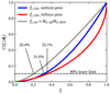 |
Fig. 1. Cumulative posterior probability of the BNS successful jet incidence. The solid red (blue) line refers to the fraction fj, GW of GW-detectable BNS mergers that produce a successful jet, based on having observed the single successful event GW170817 and adopting the Jeffreys (uniform) prior. The solid grey line refers to the jet incidence fj, tot in the entire BNS merger population, based on the ratio of the local rate of short GRB jets R0, SJ to the BNS rate R0, BNS. The implied 90% credible lower limits are annotated. |
2.2. Whole population: SGRB versus BNS local rate
Another route to constraining fj is that of comparing the local rate density R0, SJ of short GRB jets (that is, the beaming-corrected SGRB rate density at z = 0) to that of BNS mergers, R0, BNS. The resulting jet incidence estimate fj, tot = R0, SJ/R0, BNS then applies to all binaries (in contrast with that obtained in the previous section, which applies to the subpopulation of GW-detectable binaries). In a recent manuscript (Abbott et al. 2021a) describing compact binary merger population analyses including data from the GWTC-3 catalogue (Abbott et al. 2021b), the LIGO-Virgo-KAGRA (LVK) Collaboration found local BNS rates in the range R0, BNS ∈ [10 − 1700] Gpc−3 yr−1 (union of the 90% credible intervals obtained through different analyses), the broad range being partly due to the highly uncertain mass distribution. An independent estimate, based on a larger sample of events, can be made based on known Galactic double neutron stars (Kim et al. 2003). A recent study (Grunthal et al. 2021; see also Pol et al. 2020), which includes observational insights on the beam shape and viewing geometry of the PSRJ1906+0746 pulsar (which contributes significantly to the total rate), finds a Milky Way BNS merger rate  (maximum a posteriori and 90% credible range). Assuming a Milky-Way-Equivalent galaxy density ρMWEG = 0.0116 ± 0.0035 Mpc−3 in the local Universe (Abadie et al. 2010; Kopparapu et al. 2008, assuming a one-sigma local star formation rate uncertainty of ∼30%, Madau & Fragos 2017), this translates to
  (median and 90% credible range, blue line in Fig. 2). In what follows, we adopt this BNS merger rate estimate as our reference value2.
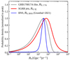 |
Fig. 2. Posterior probability distribution on the local rate density of GRB170817A-like events (grey solid line, Eq. (B.1)), SGRB jets in general (regardless of orientation, red solid line, Eq. (5)), and BNS mergers (as determined from observations of Galactic systems, blue solid line, Grunthal et al. 2021). |
The local SGRB jet rate density is poorly constrained due to the inherent difficulty in disentangling the luminosity function and redshift distribution of the cosmological SGRB population, given the current low number of events with a measured redshift, the complexity of selection effects, and the fact that it is essentially impossible to constrain the low-end of the luminosity function (roughly below 5 × 1049 erg s−1). This emerges clearly from the diversity of local rate values present in the literature (Abbott et al. 2022; Mandel & Broekgaarden 2022; Tan & Yu 2020; Liu & Yu 2019; Sun et al. 2017; Ghirlanda et al. 2016; Wanderman & Piran 2015; Coward et al. 2012). The uncertainty on the beaming-corrected rate density is exacerbated by the difficulty in determining the average beaming factor (and its likely dependence on distance) from the available data. Nevertheless, here we show that a robust lower limit on R0, SJ can be set based on the single-event rate of GRB170817A, as follows. Let Veff be the effective comoving volume over which Fermi/GBM is sensitive to an event with the same intrinsic properties as GRB178017A. The rate density R0, 17A that can be derived conservatively assuming GBM to have observed a single SGRB jet in that volume over its entire time of operation T = 13 yr, neglecting any beaming factor, is then a strict lower limit to R0, SJ. By carefully modelling the GBM sensitive volume based on the peak fluxes of observed short GRBs (as described in Appendix B) we obtain the posterior distribution on R0, 17A shown by the red line in Fig. 2, whose median and 90% credible interval are  (in agreement with e.g. Della Valle et al. 2018). Given this piece of information, our knowledge of R0, SJ can be modelled as
 (5)
(5)
where Θ is the Heaviside step function, that is
 (6)
(6)
We use the above-mentioned R0, 17A posterior as our prior π(R0, 17A), and adopt a log-uniform prior  on the SGRB jet rate density, which is a conservative choice as it favours values closer to the lower limit R0, 17A, and hence lower values of fj, tot. The result is shown in Fig. 2, along with the posterior on R0, 17A and that on R0, BNS based on Grunthal et al. (2021).
Finally, we compute the fj, tot posterior distribution as the ratio distribution of the R0, SJ and R0, BNS distributions, with the additional constraint fj, tot ≤ 1, namely
 (7)
(7)
where δ is the Dirac delta function and dtot represents the data which inform our estimates of R0, SJ and R0, BNS and, hence, the above posterior on fj, tot.
To evaluate Eq. (7) in practice, we produce  samples by the following procedure: (1) we extract an R0, SJ, i sample from a log-uniform distribution in the range 10−1 − 104 Gpc−3 yr−1 (that is, a broad enough range as to cover the support of both R0, 17A and R0, BNS), and an R0, 17A, i sample from the red distribution in Fig. 2; (2) if R0, SJ, i < R0, 17A, i we go back to (1); (3) we extract an R0, BNS, i sample from the blue distribution in Fig. 2; (4) if fj, tot, i = R0, SJ, i/R0, BNS, i > 1 we reject the sample and go back to (1), otherwise we store it. The resulting cumulative fj, tot distribution is shown by the grey line in Fig. 1, while two approximations of the probability density are shown in Fig. 3. The implied 90% credible lower limit on fj is 21% (2.4% at 3σ). As shown in Fig. 3, the associated probability density is well approximated by a power law
 (8)
(8)
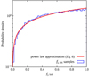 |
Fig. 3. Posterior distribution on the fraction fj, tot of BNS mergers accompanied by jets, computed as described in Sect. 2.2. The blue histogram shows the distribution of samples constructed as described in the text, that approximate Eq. (7), while the red line shows the analytical approximation |
with a best fit value γ = 0.42.
We neglect the potential contribution of neutron star – black hole mergers to the beaming-corrected local rate density of SGRB jets. This is justified by the fact that the intrinsic BNS and neutron star – black hole rates are comparable – Abbott et al. (2021c) – and most likely only a small fraction of the latter result in the tidal disruption of the neutron star, given the expected dearth of rapidly spinning BHs in these systems (see e.g. Broekgaarden et al. 2021 and Zappa et al. 2019). Other works take the alternative route of constraining the beaming factor (or the angular dependence of the jet emission properties) from the comparison of the observed rates of BNS mergers and SGRBs (e.g. Williams et al. 2018; Biscoveanu et al. 2020; Farah et al. 2020; Hayes et al. 2020), or of estimating the future joint BNS-SGRB detection rates as a function of such a factor (e.g. Chen & Holz 2013; Clark et al. 2015).
3. Modelling the jet incidence
3.1. Blandford-Znajek jet-launching conditions
The gamma-ray burst jet-launching mechanism is still under debate (see Salafia & Giacomazzo 2021 for a recent discussion and Kumar & Zhang 2015 for a review). In the case of a binary neutron star merger progenitor, the possible mechanisms are restricted to those compatible with the characteristics of the merger remnant: depending on the component neutron star masses and EoS, the merger can lead either to the prompt formation (i.e. happening on a dynamical timescale) of a black hole (BH) or to a proto-neutron star (Burrows & Lattimer 1986). If the mass Mrem of the latter is below the maximum mass MTOV that can be supported against collapse in a non-rotating neutron star, it will evolve to an indefinitely stable neutron star (NS); if the mass is above MTOV, but below the mass Mmax, rot that can be supported by uniform rotation at the mass-shedding limit (Goussard et al. 1997), the remnant is said to be a ’supra-massive’ neutron star (SMNS) and it can survive until electromagnetic spin-down eventually leads to collapse to a BH; if Mrem > Mmax, rot, the proto-neutron star can still be supported (Goussard et al. 1998) for a short time (typically ≲100 ms) by differential rotation before collapsing, in which case it is termed a ‘hyper-massive’ neutron star (HMNS).
Jets launched by neutron stars are observed in our Galaxy (e.g. Pavan et al. 2014; van den Eijnden et al. 2018) and several authors have argued that a rapidly spinning, highly magnetised proto-neutron star merger remnant may be able to launch a relativistic jet (e.g. Usov 1992; Thompson 1994; Thompson et al. 2004; Metzger et al. 2011; Mösta et al. 2020). On the other hand, the neutrino-driven (Dessart et al. 2009; Perego et al. 2014) and magnetically driven (Ciolfi & Kalinani 2020) winds produced by a proto-neutron star during its early evolution are likely to load the surrounding environment with too many baryons, preventing a putative jet from reaching relativistic speeds (e.g. Ciolfi 2020).
If the remnant is a BH (or it collapses to a BH in a time much shorter than the accretion timescale), following the amplification of the magnetic field by Kelvin-Helmholtz instabilities triggered at merger (Obergaulinger et al. 2010; Kiuchi et al. 2015; Aguilera-Miret et al. 2020) and the development of a large-scale ordered magnetic field configuration with a non-negligible poloidal component, the Blandford-Znajek jet-launching mechanism (Blandford & Znajek 1977; Komissarov 2001; Tchekhovskoy et al. 2010) can operate, possibly enhanced by energy deposition from the annihilation of neutrino-antineutrino pairs emitted by the inner accretion disc (Eichler et al. 1989 – even though this cannot be the dominant source of jet power, as found by Just et al. 2016).
Given the difficulties with the proto-neutron star central engine, in this work we assume that only a BH remnant (possibly, but not necessarily, formed after a HMNS phase) can launch a relativistic jet. Very broadly speaking, the conditions for the Blandford-Znajek mechanism to operate are the presence of a spinning BH, an accretion disc with a large-scale ordered magnetic field, and a low-density funnel above the BH (along its rotation axis). Given the particular accretion conditions in the BNS post-merger phase and the expected predominantly toroidal configuration of the magnetic field in the disc (Kiuchi et al. 2014; Kawamura et al. 2016), the accretion-to-jet energy conversion efficiency η = Ejet/(Mdiscc2) of the Blandford-Znajek mechanism in these systems (Christie et al. 2019) is likely quite low, η ∼ 10−3, as found in numerical relativity simulations (Ruiz et al. 2018) and in agreement with the estimate that can be made based on GW170817 (Salafia & Giacomazzo 2021). Assuming this efficiency, in order to produce a (short) gamma-ray burst jet with a total energy in the typical (Fong et al. 2015) range Ejet ∼ 1049 − 1050 erg, a disc mass of about Mdisc ∼ 0.01 − 0.1 M⊙ is needed.
Based on these arguments, we assume GRB jet launching to be possible only for HMNS or prompt BH remnants3, provided that the accretion disc mass is, conservatively, at least Mdisc, min = 10−3 M⊙. We note that changing this to a more stringent value, e.g. Mdisc, min = 10−2 M⊙, would have a very limited impact on our results due to the steep dependence of the disc mass on the gravitational mass M2 of the secondary component in the binary (Krüger & Foucart 2020), as demonstrated in Fig. 4. For the same reason, the uncertainty in the disc mass fitting formula (which we take into account in our methods) has little impact on our results. The first condition can be restated as the requirement that the gravitational mass Mrem of the merger remnant be at least as massive as the maximum mass that can be supported by uniform rotation Mmax, rot = 1.2MTOV, where MTOV is set by the chosen neutron star matter EoS and the factor 1.2 is essentially EoS-independent4 (Breu & Rezzolla 2016).
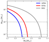 |
Fig. 4. Dependence of the disc mass on the mass of the secondary component in the binary, according to the fitting formula by Krüger & Foucart (2020). Different colours refer to different assumed equations of state, as shown in the legend. |
3.2. Determination of the remnant type
In order to compute the remnant mass Mrem, we invoke energy conservation for a merging binary with total mass M = M1 + M2, equating the energy budget of the initial state (at formally infinite binary separation) to that of the final state after the remnant has formed, in the form
 (9)
(9)
where EGW is the energy radiated in gravitational waves, Edisc is the total energy associated with the accretion disc and Eej is that associated with the ejecta (except for disc winds, which are included in Edisc), and Eν is the energy lost in neutrinos by the remnant (in the absence of a prompt BH collapse). We compute EGW using numerical-relativity-based fitting formulae from Zappa et al. (2018), which include GW mass loss all the way from the inspiral to the early post-merger phase, and are implemented in the publicly available repository bns_lum (Bernuzzi et al. 2018). The disc energy in principle comprises its rest-mass, its gravitational potential energy, the energy associated with its rotation and that contained in the magnetic field: the rotational and gravitational potential energy together amount approximately to −GMremMdisc/2Rdisc = −(Rg, rem/Rdisc)Mdiscc2/2 (where Rg, rem and Rdisc are the remnant gravitational radius and the disc radius, respectively). Since very generally Rdisc ≫ Rg, rem, these terms can be safely neglected. As stated in the previous section, during the merger the magnetic field is amplified by Kelvin-Helmholtz instabilities, reaching typical energies of ∼1051 erg (Aguilera-Miret et al. 2020). This is equivalent to less than 0.1% of a solar mass, so that this term can also be neglected. Therefore, we keep only the rest-mass contribution, that is Edisc ∼ Mdiscc2. We compute the disc rest-mass Mdisc using the fitting formula proposed in (Krüger & Foucart 2020, their Eq. (4), with their best-fit parameters, to which we refer hereafter as Mdisc, KF20). Similarly, since the typical neutron star merger ejecta velocities are subrelativistic, vej ∼ 0.1 − 0.2 c, we neglect their kinetic energy and we write Eej ∼ Mejc2. The mass Mej includes the dynamical ejecta, which we compute through the relevant fitting formula from (Krüger & Foucart 2020, their Eq. (6), with their best-fit coefficients), and potentially also winds from a long-lived neutron star remnant. The typical mass of neutrino-driven winds from a HMNS is expected (Dessart et al. 2009; Perego et al. 2014) to be of the order of 10−4 M⊙ and can be safely neglected in our treatment; winds driven by magnetically induced viscosity can be much more substantial, reaching ∼10−2 M⊙ (Ciolfi & Kalinani 2020) in sufficiently long-lived cases, but this is still well within the expected uncertainty of the fitting formula we employ for the disc mass (Krüger & Foucart 2020), and therefore we do not include this component for simplicity. Similarly, since the peak neutrino luminosity of an HMNS remnant is expected to be below Lν < 1053 erg s−1 (Dessart et al. 2009; Perego et al. 2014), and the HMNS lifetime (which is of the order of the viscous timescale in the HMNS, since differential rotation is damped by viscous angular momentum transport, e.g. Kiuchi et al. 2018) is tHMNS ≲ 0.1 s, the mass lost in neutrinos Mν = Eν/c2 ∼ LνtHMNS/c2 is well below one percent of a solar mass, and thus we set Eν = 0.
The employed fitting formulae depend on the neutron star masses and on their compactness or dimensionless tidal deformability: if an EoS is assumed, the neutron star radii can be computed from the mass-radius relation, and the tidal deformabilities from the ‘C-Love’ universal relation (Yagi & Yunes 2017). This allows one to solve Eq. (9) for Mrem = Mrem(M1, M2, θEoS), where θEoS represents a set of parameters that define the EoS. Setting Mrem < MTOV as the condition for an indefinitely stable NS remnant; MTOV ≤ Mrem < 1.2MTOV as the condition for a SMNS remnant; 1.2MTOV ≤ Mrem < Mthresh as the condition for a HMNS remnant, and Mrem ≥ Mthresh for direct collapse to a BH, one can then determine the fate of the merger remnant based on the initial binary masses and on the EoS. Here Mthresh is the threshold mass for BH direct collapse, which can be computed employing the mass ratio-dependent fitting formula given in Bauswein et al. (2021). Alternative recent formulae exist (e.g. Tootle et al. 2021; Kashyap et al. 2022; Kölsch et al. 2021), but we note that our results do not depend on this choice: the Mthresh line shown in Fig. 5 as the separation between the HMNS and BH remnant regions is only illustrative and it does not enter our assumed jet-launching conditions.
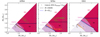 |
Fig. 5. Merger remnant and GRB launching regions on the component mass plane. The filled coloured regions correspond to different BNS merger remnants on the (M1, M2) plane, assuming different EoSs: APR4 (left-hand panel), SFHo (central panel) and DD2 (right-hand panel). Grey hatches mark masses that are above the maximum non-rotating mass supported by the EoS. The black dashed lines enclose the region where our GRB jet-launching conditions are met, computed as described in Sect. 3.1 (the blue dashed lines, shown for comparison, are computed with the approximate method described in Sect. 3.3). White circles and contours show the best fit and 90% credible contours of masses of known Galactic BNS systems whose coalescence time tmerge is shorter than a Hubble time (tH, data from Farrow et al. 2019). The orange and green contours show the 50% and 90% credible regions for the component masses in GW170817 (Abbott et al. 2019) and GW190425 (Abbott et al. 2020a), respectively, adopting low-spin priors. |
Figure 5 shows the resulting regions that correspond to different expected remnants of BNS mergers on the (M1, M2) plane, assuming three different EoSs, namely APR4 (Akmal et al. 1998), SFHo and DD2 (Hempel et al. 2012), which predict maximum masses MTOV/M⊙ = 2.19, 2.06 and 2.42, respectively (all of which are above the largest Galactic neutron star masses measured to date, Lynch et al. 2013; Fonseca et al. 2021), and radii in the range R1.4 ∈ (11.30, 13.25) km for a 1.4 M⊙ neutron star, in agreement with constraints from GW170817 (Abbott et al. 2018, 2019) and from NICER (Miller et al. 2019; Raaijmakers et al. 2019, 2020; Landry et al. 2020, with some tension in the case of DD2). The black dashed lines enclose the region where our GRB jet-launching conditions are met. The upper boundary is a horizontal line: this is due to the fact that the disc mass fitting formula by Krüger & Foucart (2020) depends only on the compactness of the least massive neutron star, but we verified that a weak dependence on the mass of the most massive NS is reflected in other recent disc mass fitting formulae (Dietrich et al. 2020; Barbieri et al. 2021), which also lead to upper boundaries that are close to horizontal. The blue dashed lines show the result obtained by adopting the simplified EoS dependence described in the next section, plugging in the MTOV and R1.4 values implied by each EoS. Confidence contours for the component masses of GW170817 (Abbott et al. 2019) and GW190425 (Abbott et al. 2020a) are shown for reference. For the two softer equations of state, APR4 and SFHo, our jet-launching conditions are most likely satisfied in GW170817 and also in a significant fraction of Galactic BNS (4/10 for APR4; 6/10 for SFHo). If the stiffer DD2 EoS is adopted, then GW170817 clearly falls in the supra-massive neutron remnant region: if such an EoS were found to best represent neutron star matter, then the jet-launching mechanism that operated in the case of GW170817 would have to be something different from Blandford-Znajek.
3.3. Approximate two-parameter EoS dependence
Our assumed jet-launching conditions require, in practice, the merger remnant mass to satisfy Mrem > 1.2MTOV and the disc mass to satisfy Mdisc > Mdisc, min. A rough idea of where the former separation line stands can be obtained by writing a simplified remnant mass equation Mrem ∼ M − EGW/c2 − Mdisc, thus neglecting the dynamical ejecta mass (in addition to all other terms which we already neglect for the reasons explained in the previous section). This leads to a critical total mass for jet launch Mcrit ∼ (1.2MTOV + Mdisc)/(1 − ηGW), where ηGW = EGW/(Mc2). This places the critical mass in the range Mcrit/M⊙ ∈ [2.4, 3.26] for 2 ≤ MTOV/M⊙ ≤ 2.5, Mdisc ≤ 0.1 M⊙ and ηGW ≤ 0.05. Assuming equal masses, the component masses are therefore in the range M1, 2/M⊙ ∈ [1.2, 1.63]. For most viable EoSs, the NS radius is approximately constant within this mass range (e.g. Özel & Freire 2016), so that one can quite safely assume it to be equal to R1.4, i.e. that of a reference 1.4 M⊙ NS. Fixing the NS radius to this value, the compactness of the secondary can be determined from its mass. The disc mass computed using the Mdisc, KF20 fitting formula thus becomes a function of M2 only. A reasonable estimate of ηGW can be obtained as the absolute value of the Keplerian orbital energy of two point masses (M1, M2), at a 2R1.4 separation, divided by Mc2, which gives ηGW ∼ νGM/4R1.4c2, where ν = M1M2/M2 = (2 + q + q−1)−1 is the symmetric mass ratio. This effectively reduces the EoS dependence of Mcrit to only two parameters, namely θEoS = {R1.4, MTOV}. In Fig. 5 we show the Mcrit obtained with this method (oblique blue dashed lines). To obtain also the line beyond which Mdisc < 10−3 M⊙ (horizontal blue dashed lines), we employed the Mdisc, KF20 fitting formula keeping the NS radius fixed at R1.4. These examples show that the approximate method yields results that differ from the more accurate ones (black dashed lines) at the percent level. In the remainder of this work, we adopt the simpified 2-parameter dependence described above.
3.4. EoS priors and jet probability on the (M1, M2) plane
In our framework, the currently available information on the EoS needs to expressed in the form of priors on R1.4 and MTOV. For both quantities there exists a variety of recent constraints that use either electromagnetic or GW information, or try to combine both.
The very thorough and complete recent work by Miller et al. (2021) based on X-ray pulsar radius measurements from NICER and XMM-Newton combined with GW constraints found R1.4 = 12.45 ± 0.65 km (one sigma) consistently using three independent frameworks, showing that the result is robust against systemtatics. We therefore use a normal distribution with a mean 12.45 km and standard deviation 0.65 km as our prior on R1.4.
The available constraints on MTOV are more uncertain and model-dependent, as can be partly appreciated by looking at the posteriors on MTOV reported in Fig. 6, which have been obtained in recent works by three different groups using four different frameworks. On the other hand, a model-independent constraint is set by the mass of the heaviest known pulsar5 PSRJ0740+6620 (Cromartie et al. 2020), whose measurement has been recently refined (Fonseca et al. 2021) to MPSR = 2.08 ± 0.07 M⊙ based on high-cadence data from the Green Bank Telescope (GBT) and the Canadian Hydrogen Intensity Mapping Experiment (CHIME). Moreover, the observation of a jet in GW170817 implies, according to our jet-launching conditions, that the remnant gravitational mass Mrem, GW17 was above 1.2MTOV. Within our framework, after fixing R1.4 we can compute the posterior probability on Mrem, GW17 using the procedure described in Sect. 3.2 and the publicly available posterior samples on the GW170817 component masses (Abbott et al. 2019, where we conservatively adopted the samples from the high-spin prior analysis, which yield broader posteriors). Then, the conditions MTOV > MPSR and 1.2MTOV < Mrem, GW17 lead to a prior on MTOV conditioned on a particular value of R1.4 that can be expressed as
![Mathematical equation: $$ \begin{aligned} \begin{aligned}&\pi (M_{\rm TOV}\,|\,R_{1.4},\xi _{\rm d}) \propto \\&\Phi _{M_{\rm PSR}}(M_{\rm TOV})\left[1-\Phi _{M_{\rm rem,GW17}}(1.2 M_{\rm TOV})\right], \end{aligned} \end{aligned} $$](/articles/aa/full_html/2022/10/aa43260-22/aa43260-22-eq18.gif) (10)
(10)
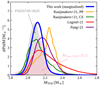 |
Fig. 6. Our prior on MTOV compared to recent model-dependent constraints in the literature. The blue thick line shows the marginalised MTOV prior we adopt in this work, which is constructed using the latest PSRJ0740+6620 mass measurement (Fonseca et al. 2021, grey filled area) as a lower limit and the remnant mass of GW170817 divided by 1.2 (pink filled area) as an upper limit (see text for an explanation). The remaining lines show results that combine multi-messenger constraints within different frameworks: the orange and green lines show the results obtained by Raaijmakers et al. (2021a) adopting their piecewise-polytropic (PP) and sound-speed (CS) parametrised EoS models, respectively; the dark red line shows the result from Legred et al. (2021) based on a non-parametric, Gaussian-processes-based EoS model; the purple line shows the result from Pang et al. (2021), who adopt an EoS model informed by chiral effective field theory. |
where Φx(m) represents the cumulative posterior distribution of x evaluated at m. To account for the uncertainty in the disc mass fitting formula, we introduced in the above formulation an additional nuisance parameter ξd, so that Mdisc(M2, R1.4, ξd) = ξdMdisc, KF20(M2, R1.4). The prior on this parameter is defined to reflect the 50% uncertainy in the disc mass fitting formula as estimated by Krüger & Foucart (2020), that is
 (11)
(11)
where
![Mathematical equation: $$ \begin{aligned} \mathcal{N} _{\mathrm{\mu },\mathrm{\sigma }}(x)\propto \exp \left[-\frac{1}{2}\left(\frac{x - \mu }{\sigma }\right)^2\right]. \end{aligned} $$](/articles/aa/full_html/2022/10/aa43260-22/aa43260-22-eq20.gif) (12)
(12)
The joint prior on MTOV, R1.4 and ξd is therefore
 (13)
(13)
where
 (14)
(14)
as explained above.
Figure 6 shows the marginalised prior on MTOV, that is, Eq. (13) marginalised over R1.4 and ξd (thick blue solid line), compared to recent multi-messenger constraints on MTOV from the literature. The comparison shows that our prior on MTOV is compatible with other recent works in the literature, but with less support at high masses in most cases, as a consequence of the assumption on the GW170817 remnant. We note that similar results based on analogous arguments have been presented by Rezzolla et al. (2018), Shibata et al. (2019), and Annala et al. (2022), for example.
Using the above-defined joint prior, we can compute the probability that a M1, M2 binary satisfies our jet-launching conditions as
 (15)
(15)
where Θj(M1, M2, θEoS) = 1 if our jet-launching conditions are met, and Θj = 0 otherwise. More explicitly,
 (16)
(16)
where we stress that Mrem and Mdisc depend on the merging binary component masses, the EoS and the nuisance parameter ξd. The result of Eq. (15) for our choice of EoS priors is shown in Fig. 7. The lighter the colour, the more likely our jet-launching conditions are met, given our present knowledge about the EoS6. For systems located in the dark lower-left corner of the plot, we can confidently predict that their remnant will not collapse to a BH on a short timescale, preventing the Blandford-Znajek mechanism from operating. Jet launching by the same mechanism is also confidently excluded for systems in the upper-right dark corner, as these produce negligible accretion discs. The fj, tot (or fj, GW) lower limits from Sect. 2 therefore lead qualitatively to the conclusion that we can exclude that the large majority (indicatively more than 90%) of BNS systems are located in the darkest regions of this plot. The absence of observed BNS mergers or Galactic double neutron stars in these regions is therefore not due to selection effects, and models that predict a large fraction of low-mass systems, such as many population synthesis models (e.g. Fryer et al. 2012; Dominik et al. 2012; Vigna-Gómez et al. 2018; Mapelli & Giacobbo 2018), are therefore in clear tension with these results.
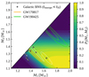 |
Fig. 7. Probability that a BNS would satisfy our jet-launching conditions (Eq. (15)) as a function of the component masses M1 and M2, given our present knowledge of the EoS (encoded in the priors defined in Sect. 3.4). The masses of Galactic BNS systems that merge within a Hubble time and the two GW-detected BNS are shown for comparison, in the same way as in Fig. 5. |
4. Inference on the BNS mass distribution and the EoS based on the jet incidence
4.1. Derivation
Our jet-launching conditions depend on the component masses M1 and M2 as well as on the EoS through MTOV and the dependence of the disc mass on the compactness of the secondary neutron star. For a fixed mass distribution d2P/dM1dM2 of BNS mergers and EoS, one can compute fj, tot directly from
 (17)
(17)
where we use the tilde ( ) to distinguish this functional (which depends on the mass distribution and on the EoS) from the fj, tot observable. Similarly, one could compute the jet incidence in GW-detected binaries as
 (18)
(18)
where Veff represents the GW detector sensitive volume for a binary with masses M1 and M2, averaged over all extrinsic parameters. For the present detector network, whose BNS range is bound to z ≪ 1 and whose signal-to-noise ratio is dominated by the inspiral phase, a good approximation is  , where Mc = (M1M2)3/5/(M1 + M2)1/5 is the chirp mass (e.g. Mandel et al. 2019). In what follows, we use fj to indicate either fj, tot or fj, GW (depending on which one of the constraints shown in Fig. 1 is used), and
  to indicate
  or
or  accordingly; we also use d to indicate the data that is used to constrain fj, that is the information on the jet incidence in GW-detected BNS binaries (Sect. 2.1, i.e. the fact that GW170817 launched a jet, which we denote hereon by dGW) or that on the SGRB and BNS local rate densities (Sect. 2.2, i.e. dtot). Expressing the mass distribution in a parametric form with a set of parameters θm, and again the EoS with a set of parameters θEoS (we include in this set, for ease of presentation, also the nuisance parameter ξd), we can formally use Bayes’ theorem to infer posteriors on these parameters from fj, obtaining
 (19)
(19)
where π(θm, θEoS) is the prior7 on θm and θEoS, and the likelihood term is simply
 (20)
(20)
Since the latter is not known exactly, but it is in turn inferred from d, we have
 (21)
(21)
which, using Eq. (20), simplifies to
 (22)
(22)
This equation expresses the joint constraint on the EoS and mass distribution parameter space that can be set by our arguments. For current constraints, using Eqs. (2) and (8) and conservatively adopting a uniform prior on fj, this can be finally written as
![Mathematical equation: $$ \begin{aligned} P({\boldsymbol{\theta }}_{\rm m},{\boldsymbol{\theta }}_{\rm EoS}\,|\,\boldsymbol{d}) \propto \left[ \tilde{f}_{\rm j}({\boldsymbol{\theta }}_{\rm m},{\boldsymbol{\theta }}_{\rm EoS})\right]^\gamma \pi ({\boldsymbol{\theta }}_{\rm m},{\boldsymbol{\theta }}_{\rm EoS}), \end{aligned} $$](/articles/aa/full_html/2022/10/aa43260-22/aa43260-22-eq36.gif) (23)
(23)
where γ = 1 if fj = fj, GW (see Sect. 2.1) or γ = 0.42 if fj = fj, tot (see Sect. 2.2). The somewhat shallower constraint on fj, tot with respect to fj, GW is partly compensated by the Veff term in Eq. (18) but, as we show in the following section, the fj, GW is still the most constraining one between the two, given the currently available data.
4.2. Mass distribution constraints
The formalism derived in the previous section can be used to investigate the parameter space of a mass distribution model. Given our a priori knowledge of the EoS, encoded in the prior, we can marginalise Eq. (23) over θEoS to formally obtain the posterior on the mass distribution parameters, namely
 (24)
(24)
Taking a uniform prior on the mass distribution parameters, π(θm)∝1, this essentially reduces to averaging  over the EoS uncertainty for a fixed choice of θm. Figure 8 shows the latter quantity for a simple mass distribution model where both binary component masses are sampled from the same Gaussian distribution with mean μm and σm. We consider wide ranges for these parameters, that is 1 ≤ μm/M⊙ ≤ 2 (encompassing the range of observed neutron star masses) and 0.01 ≤ σm/M⊙ ≤ 0.5 (from very narrow to very wide Gaussians over the considered mass range). The marginalisation over the EoS parameters is performed using our simplified two-parameter EoS dependence (Sect. 3.3), adopting the priors introduced in Sect. 3.4, limiting the NS masses to the range M1, 2 ∈ [1 M⊙, MTOV]. Filled contours show the result obtained using fj = fj, GW, while empty contours show the corresponding result when adopting the fj = fj, tot alternative constraint.
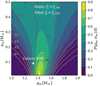 |
Fig. 8. Constraints on the parameters of a Gaussian BNS mass distribution model. Filled contours show the posterior probability density on the μm (mean) and σm (standard deviation) parameters of a Gaussian mass distribution model (assuming random pairing) obtained using fj = fj, GW, i.e. the constraint based on the association of GW170817 and GRB170817A (Sect. 2). Empty contours show the corresponding result for fj = fj, tot, i.e. the constraint based on the relative SGRB and BNS local rate densities (Sect. 2.2). The white star marks parameter values (μm, σm) = (1.33, 0.09) M⊙, representative of the main peak of the observed Galactic BNS mass distribution (Özel & Freire 2016). |
This shows that a narrow (σm ≲ 0.2 M⊙) Gaussian distribution with μm ≲ 1.3 M⊙ or μm ≳ 1.6 M⊙ is strongly disfavoured due to the very low implied jet incidence, given the available information on the EoS and the jet incidence, and consistently when using either of the constraints we considered (that is, dGW or dtot). On the other hand, parameters representative of the main peak of the observed Galactic BNS population (white star in Fig. 8) are consistent with the constraints.
Given the fact that the analysis of GW-detected BNS (Abbott et al. 2021a; Landry & Read 2021), radio-detected Galactic BNS (Farrow et al. 2019) and both populations together (Galaudage et al. 2021) currently disfavour a narrow-peaked mass distribution, we also tested a different parametric form, that is, a power law mass distribution model where both components are sampled from a power law P(m | α, Mmin, MTOV)∝mα with Mmin ≤ m ≤ MTOV, where m is the mass of either component. We consider a wide range of slopes −20 ≤ α ≤ 10, and we take 1 ≤ Mmin/M⊙ ≤ 1.25, with the upper bound being limited by the lightest observed masses Galactic neutron stars (Farrow et al. 2019).
Figure 9 shows the resulting constraint on the (α, Mmin) plane, with the same colour coding as for the Gaussian mass distribution.
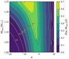 |
Fig. 9. Constraints on the parameters of a power law BNS mass distribution model. Colours and lines have the same meaning as in Fig. 8. |
It is instructive to project both results on the actual mass distribution space. We stress that we assume the component masses to be sampled from the same distribution (and randomly paired) which we refer to as Pm(m | θm). The implied primary mass distribution is therefore
 (25)
(25)
and similarly for the secondary mass distribution. We keep the same uniform priors as in Figs. 8 and 9, and we use the constraint on fj = fj, GW.
Figure 10 shows the resulting mass distribution constraints. The credible bands in the figure are obtained as follows: we sampled the θm posterior (computed according to Eq. (24)) and constructed the P(m | θm) curves corresponding to the samples. For each fixed value of m, the 50% (resp. 90%) credible band is comprised between the 25th and the 75th (resp. 5th and the 95th) percentiles of the values of these curves at m. Similarly, the thick solid lines represent the medians of these values. The cut-offs below 1 M⊙ and above 2.2 M⊙ are determined by our priors; in between this range, the result shows some improvement with respect to the priors and generally disfavours narrow mass distributions. The clearest feature, common to the two parametrisations (as is particularly visible in the comparison panel), is the requirement of a non-negligible probability for masses in the 1.3 − 1.6 M⊙ range, which are particularly well-positioned in terms of satisfying our jet-launching conditions, as shown in Fig. 7. This is in good agreement with the position and width of the main mass peak as found by Galaudage et al. (2021). In Appendix C we show a comparison of these results to those from the recently circulated preprint on the LIGO/Virgo GWTC-3 population study by Abbott et al. (2021a).
 |
Fig. 10. Mass distribution constraint. In each panel, filled contours show the 90% and 50% credible regions of the probability distribution P(m | θm) from which both M1 and M2 are sampled, while the thick solid line shows the median distribution at each m. The dj, GW constraint is used. Grey dashed lines show the edges of the corresponding 90% and 50% credible regions when using only the priors. Left-hand panel: the result for the power law mass distribution model, the central panel shows that for the Gaussian model, and the right-hand panel compares the two results with a log-scale vertical axis, to emphasise the lower 90% contour. |
4.3. EoS constraints
The posterior in Eq. (23) can also be marginalised over the mass distribution parameters, to obtain constraints on the EoS given the knowledge of the mass distribution. Unfortunately, the current uncertainties on the jet incidence and mass distribution are too large, and this simply returns the EoS priors (which are already quite informative).
To give a basic illustration of the relevance of this kind of constraint in the future, we consider the following example. We adopt the power law mass distribution model described above, with a uniform prior on Mmin between 1.0 M⊙ and 1.3 M⊙, and a uniform prior on α between −9 and 3.3, matching the 90% credible ranges from the GWTC-3 population study (Abbott et al. 2021a). This therefore roughly represents the current uncertainty on the NS mass distribution in merging stellar-mass compact object binaries. As a way of representing a hypothetical future in which the jet incidence is known with relatively small uncertainty, we assume the posterior probability on the jet incidence in GW-detectable binaries fj, GW to be represented by a Gaussian with standard deviation σf = 0.05 (which represents roughly a 6-fold improvement over the current uncertainty, see Fig. 1) and two possible mean values, μf = 0.25 and μf = 0.75. Equation (22) then becomes
 (26)
(26)
The marginalised distributions P(MTOV, R1.4 | dGW) for the two choices of μf are shown in Figs. 11 and 12.
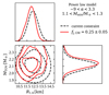 |
Fig. 11. Illustrative constraints on the EoS parameters assuming the power law mass distribution model with uniform priors on 1.1 ≤ Mmin/M⊙ ≤ 1.3 and −9 ≤ α ≤ 3.3, matching the 90% credible ranges of the GWTC-3 NS mass distribution constraint (Abbott et al. 2021a), and using a hypothetical future constraint on the jet incidence P(fj, GW | dGW)∝𝒩0.25, 0.05(fj, GW). |
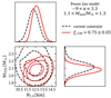 |
Fig. 12. Same as Fig. 11, but assuming a jet incidence constraint with a different mean, that is P(fj, GW | dtot)∝𝒩0.75, 0.05(fj, GW). |
The results show that the posterior probability on the EoS parameters is sensitive to the value of fj, GW even when the BNS mass distribution is relatively poorly known. We conclude that in the near future, when the BNS mass distribution (plus the local rate and possibly the jet incidence) will be better constrained thanks to more GW observations, this methodology will be able to place interesting constraints on the EoS parameters. This is in agreement with Fryer et al. (2015), who first discussed the possiblity to constrain MTOV from the jet incidence in GW-detectable BNS mergers.
5. Discussion and conclusions
The successful jet in GW170817 not only provided strong evidence in support of the long-held binary neutron star progenitor scenario for short gamma-ray bursts, but also clearly indicated that the launch of a relativistic jet is most likely a common outcome of these kinds of mergers. In this work, we have shown how the fraction of BNS mergers that launch an ultra-relativistic jet can be used to place a joint constraint on the binary neutron star mass distribution and on the neutron star matter EoS, under the assumption that the jet-launching mechanism requires the presence of an accretion disc with a non-negligible mass and the collapse of the merger remnant to a BH within a fraction of a second (i.e. a supra-massive or stable neutron star remnant is assumed not to yield SGRBs).
Based on the presence of a jet in GW170817 and adopting a simple binomial likelihood and a uniform prior, we derived a lower limit fj, GW > 32% (90% credible level) on the incidence of jets in GW-detected binary neutron stars. By comparing the lower limit on the local short gamma-ray burst rate density that can be placed by the detection of GRB170817A by Fermi/GBM and the local binary neutron star merger rate density estimated by Grunthal et al. (2021) based on Galactic double neutron stars, we constrained the jet incidence in the whole population to be fj, tot > 20%. This constraint is weaker than the finding of fj, tot > 40% (90% credible level) by Sarin et al. (2022), a pre-print – now published – that appeared while this work was nearing submission. However, the quantitative discrepancy is likely due to the reliance by Sarin et al. (2022) on the inferred local SGRB rate density estimated by Coward et al. (2012) and Wanderman & Piran (2015) – which most likely suffer from systematics due to the uncertain luminosity function (especially at the low end) and redshift distribution of events (see Sect. 2.2) – and their assumption that promptly collapsing BNS merger products without a signifiant accretion disc could still launch a jet and power a SGRB.
Comparing these results with the predicted jet incidence in a Blandford & Znajek (1977) jet-launching scenario, assuming EoS priors informed by the latest multi-messenger constraints, we can exclude mass distributions with an overwhelming fraction of low-mass (≲1.3 M⊙) neutron stars (as predicted by many population synthesis models, especially those that adopt the Fryer et al. 2012 ‘rapid’ supernova prescription). This finding qualitatively agrees with Sarin et al. (2022; their Fig. 1). Similarly, a mass distribution dominated by high-mass (≳1.6 M⊙) components is strongly disfavoured. We caution that this conclusion critically depends on the assumed jet-launching conditions: if an alternative magnetar central engine scenario (though theoretically less favoured) was adopted, these conclusion would be significantly altered.
The method can also be used, in principle, to place constraints on the EoS, but the current data are insufficient to make this methodology competitive. Nevertheless, in Sect. 4.3 we provided a first illustration of how this will improve with future tighter constraints on the jet incidence.
Given the relatively weak constraints that we obtain with the currently available data, this work must be regarded primarily as a proof of concept. In the near future, several new binary neutron stars are expected (Abbott et al. 2020b) to be detected through gravitational waves in the upcoming O4 and O5 observing runs of the GW detector network (which now includes KAGRA, Somiya 2012). In addition to that, new binary pulsars are being discovered in radio surveys (Han et al. 2021; Pan et al. 2021; Good et al. 2021; Agazie et al. 2021) at an increasing rate thanks to the steady improvements in both technology and data analysis techniques. Last, but not least, our understanding of selection effects that shape the properties of the observed radio pulsar population is advancing (Chattopadhyay et al. 2020). All of these advances are going to positively impact the constraints on fj, GW and fj, tot (Fig. 1) and the θm and θEoS constraints that can be derived through the presented methodology.
New gravitational-wave detections of binary neutron star mergers will also open the possibility of directly using the information on the presence of a jet in each event (see Appendix A for an extension to uncertain jet associations) in population studies. In a modelling framework such as that described by Mandel et al. (2019), the jet-launching condition (represented by the Θj term, Eq. (16)) could be used, in conjunction with the available information on the presence or absence of a jet in each GW-detected BNS merger, to constrain the parameters of single events in the population and, as a result, of global population parameters (i.e. hyperparameters) such as θm and θEoS. This can complement methods that exploit information on kilonova ejecta masses (Li & Paczyński 1998; Metzger 2019) and SGRB afterglow observations to augment the information that can be obtained from the gravitational-wave data (e.g. Hotokezaka et al. 2019; Radice & Dai 2019; Lazzati & Perna 2019; Barbieri et al. 2019; Coughlin et al. 2019; Dietrich et al. 2020; Breschi et al. 2021; Raaijmakers et al. 2021b). In this context, multi-messenger observations of BNS mergers close to the boundaries of the currently viable parameter space for jet launching would be particularly informative: as an example, the observation of a clear jet signature (or a tight constraint on its presence) in a system whose masses lie in the region where jet launching is most uncertain (regions where Pj ∼ 0.5 in Fig. 7) would have the highest impact on the results that can be obtained with the presented method. Conversely, observations that clearly contradict the jet-launching conditions adopted in this work (such as a jet-less system with masses in the Pj ∼ 1 region in Fig. 7, or a jet-launching system with masses in the dark blue regions of the same figure) would point to the need for a revision in the assumed jet-launching conditions.
These works provide support for a large fj based on the comparison of the single-event rate of GW170817 with the observed short gamma-ray burst rate.
Double neutron star binaries containing an observable pulsar clearly represent only a subpopulation of merging binaries. While Grunthal et al. (2021) carefully account for selection effects and for the pulsar lifetimes in inferring the total number and merger rate of Galactic double neutron stars from the observed population, they do not account for a possible fraction of the population that is not currently detected by radio surveys, which may form through different channels (e.g. Vigna-Gómez et al. 2021) and may account for massive systems such as GW190425 (Abbott et al. 2020a). Such systems, on the other hand, are unlikely to constitute a dominant fraction of the total (as also suggested by the relative rate densities of GW170817 and GW190425), and thus the systematic error that stems from using the Grunthal et al. (2021) rate as a proxy for the total BNS rate is most likely less than a factor of 2. The uncertainty in the conversion between the Galactic and local volumetric merger rates incorporated into our analysis may therefore underestimate the total merger rate uncertainty.
We note that the inclusion of prompt BH collapse cases is justified by the fact that sufficiently asymmetric systems can produce massive accretion discs by the tidal disruption of the secondary neutron star, regardless of the nature of the remnant (Bernuzzi et al. 2020).
A small deviation from this quasi-universal value is expected for equations of state with a first-order phase transition (e.g. Bozzola et al. 2019).
The PSRJ0740+6620 pulsar is inferred to spin at a frequency of roughly 350 Hz (Cromartie et al. 2020), which is up to 25% of the Keplerian (i.e. mass shedding) frequency for viable EoSs (see Haensel et al. 2009). Rotation at such a rate increases the maximum mass that can be supported by the EoS by up to 0.85% (Breu & Rezzolla 2016). We neglect this small correction here, as it is well below our uncertainties.
We note that the value of Pj averaged over the GW170817 joint component mass posterior (adopting the low-spin-prior samples from Abbott et al. 2019) is 78%. This is not 100% because the information that GW170817 successfully launched a jet enters only through the prior on MTOV and it cannot be applied self-consistently to the GW170817 masses within the present method. An alternative approach that solves this issue is outlined in the discussion section.
The priors on θm and θEoS are not necessarily independent from each other, as the mass distribution parameters can for example include MTOV.
We note that the available observations themselves could have been performed in an attempt to collect conclusive evidence in favour of a jet, in case preliminary observations provided promising indications of its presence. In that sense, Pmiss can evolve as the data are collected and, in favourable cases such as GW170817, it can get close to zero (i.e. any jet in association to GW170817, if present, would not have been missed, also factoring in the indications towards a relatively small viewing angle that stem from kilonova observations, see e.g. Breschi et al. 2021). This latter statement clearly depends also on the assumed distribution of possible jet luminosities and properties in the probed bands.
In low signal-to-noise ratio events such as GW190425, the posterior is well-approximated by the universal inclination angle distribution of GW-detected binaries of Schutz (2011). Indeed, using that distribution our result changes only by a few percent.
Acknowledgments
The authors thank the anonymous referee for a very detailed and insightful report that helped in improving the presentation of the results. The authors also thank Sylvia Biscoveanu and Samuele Ronchini for insightful comments and suggestions. OS thanks Giancarlo Ghirlanda, Monica Colpi, Michele Ronchi, Annalisa Celotti and Floor Broekgaarden for helpful comments and discussions. OS acknowledges financial support from the INAF-Prin 2017 (1.05.01.88.06) and the Italian Ministry for University and Research grants 1.05.06.13 and 20179ZF5KS. IM acknowledges support from the Australian Research Council Centre of Excellence for Gravitational Wave Discovery (OzGrav), through project number CE17010004. IM is a recipient of the Australian Research Council Future Fellowship FT190100574.
References
- Abbott, R., Abbott, T. D., Acernese, F., et al. 2022, ApJ, 928, 186 [NASA ADS] [CrossRef] [Google Scholar]
- Acernese, F., Agathos, M., Agatsuma, K., & Virgo, C. 2014, CQG, 32, 024001 [Google Scholar]
- Agazie, G. Y., Mingyar, M. G., McLaughlin, M. A., et al. 2021, ApJ, 922, 35 [NASA ADS] [CrossRef] [Google Scholar]
- Aguilera-Miret, R., Viganò, D., Carrasco, F., Miñano, B., & Palenzuela, C. 2020, Phys. Rev. D, 102, 103006 [NASA ADS] [CrossRef] [Google Scholar]
- Akmal, A., Pandharipande, V. R., & Ravenhall, D. G. 1998, Phys. Rev. C, 58, 1804 [Google Scholar]
- Annala, E., Gorda, T., Katerini, E., et al. 2022, Phys. Rev. X, 12, 011058 [NASA ADS] [Google Scholar]
- Ascenzi, S., Oganesyan, G., Salafia, O. S., et al. 2020, A&A, 641, A61 [NASA ADS] [CrossRef] [EDP Sciences] [Google Scholar]
- Barbieri, C., Salafia, O. S., Perego, A., Colpi, M., & Ghirlanda, G. 2019, A&A, 625, A152 [NASA ADS] [CrossRef] [EDP Sciences] [Google Scholar]
- Barbieri, C., Salafia, O. S., Colpi, M., Ghirlanda, G., & Perego, A. 2021, A&A, 654, A12 [NASA ADS] [CrossRef] [EDP Sciences] [Google Scholar]
- Barkov, M. V., Luo, Y., & Lyutikov, M. 2021, ApJ, 907, 109 [NASA ADS] [CrossRef] [Google Scholar]
- Bauswein, A., Blacker, S., Lioutas, G., et al. 2021, Phys. Rev. D, 103, 123004 [NASA ADS] [CrossRef] [Google Scholar]
- Beniamini, P., Petropoulou, M., Barniol Duran, R., & Giannios, D. 2019, MNRAS, 483, 840 [NASA ADS] [CrossRef] [Google Scholar]
- Beniamini, P., Duque, R., Daigne, F., & Mochkovitch, R. 2020, MNRAS, 492, 2847 [NASA ADS] [CrossRef] [Google Scholar]
- Berger, E. 2014, ARA&A, 52, 43 [CrossRef] [Google Scholar]
- Bernardini, M. G., Margutti, R., Zaninoni, E., & Chincarini, G. 2012a, Mem. Soc. Astron. It. Suppl., 21, 226 [Google Scholar]
- Bernardini, M. G., Margutti, R., Mao, J., Zaninoni, E., & Chincarini, G. 2012b, A&A, 539, A3 [NASA ADS] [CrossRef] [EDP Sciences] [Google Scholar]
- Bernardini, M. G., Campana, S., Ghisellini, G., et al. 2013, ApJ, 775, 67 [NASA ADS] [CrossRef] [Google Scholar]
- Bernuzzi, S., Breschi, M., Daszuta, B., et al. 2020, MNRAS, 497, 1488 [Google Scholar]
- Bernuzzi, S., Perego, A., & Zappa, F. 2018, bns_lum git repository https://git.tpi.uni-jena.de/core/bns_lum [Google Scholar]
- Biscoveanu, S., Thrane, E., & Vitale, S. 2020, ApJ, 893, 38 [NASA ADS] [CrossRef] [Google Scholar]
- Blandford, R. D., & Znajek, R. L. 1977, MNRAS, 179, 433 [NASA ADS] [CrossRef] [Google Scholar]
- Bozzola, G., Espino, P. L., Lewin, C. D., & Paschalidis, V. 2019, Eur. Phys. J. A, 55, 149 [NASA ADS] [CrossRef] [Google Scholar]
- Breschi, M., Perego, A., Bernuzzi, S., et al. 2021, MNRAS, 505, 1661 [NASA ADS] [CrossRef] [Google Scholar]
- Breu, C., & Rezzolla, L. 2016, MNRAS, 459, 646 [NASA ADS] [CrossRef] [Google Scholar]
- Broekgaarden, F. S., Berger, E., Neijssel, C. J., et al. 2021, MNRAS, 508, 5028 [NASA ADS] [CrossRef] [Google Scholar]
- Burns, E., Connaughton, V., Zhang, B.-B., et al. 2016, ApJ, 818, 110 [NASA ADS] [CrossRef] [Google Scholar]
- Burns, E., Svinkin, D., Hurley, K., et al. 2021, ApJ, 907, L28 [NASA ADS] [CrossRef] [Google Scholar]
- Burrows, A., & Lattimer, J. M. 1986, ApJ, 307, 178 [Google Scholar]
- Chattopadhyay, D., Stevenson, S., Hurley, J. R., Rossi, L. J., & Flynn, C. 2020, MNRAS, 494, 1587 [NASA ADS] [CrossRef] [Google Scholar]
- Chen, H.-Y., & Holz, D. E. 2013, Phys. Rev. Lett., 111, 181101 [NASA ADS] [CrossRef] [Google Scholar]
- Christie, I. M., Lalakos, A., Tchekhovskoy, A., et al. 2019, MNRAS, 490, 4811 [NASA ADS] [CrossRef] [Google Scholar]
- Ciolfi, R. 2020, MNRAS, 495, L66 [NASA ADS] [CrossRef] [Google Scholar]
- Ciolfi, R., & Kalinani, J. V. 2020, ApJ, 900, L35 [NASA ADS] [CrossRef] [Google Scholar]
- Clark, J., Evans, H., Fairhurst, S., et al. 2015, ApJ, 809, 53 [NASA ADS] [CrossRef] [Google Scholar]
- Colombo, A., Salafia, O. S., Gabrielli, F., et al. 2022, ApJ, 937, 79 [NASA ADS] [CrossRef] [Google Scholar]
- Coughlin, M. W., Dietrich, T., Margalit, B., & Metzger, B. D. 2019, MNRAS, 489, L91 [NASA ADS] [CrossRef] [Google Scholar]
- Coward, D. M., Howell, E. J., Piran, T., et al. 2012, MNRAS, 425, 2668 [CrossRef] [Google Scholar]
- Cromartie, H. T., Fonseca, E., Ransom, S. M., et al. 2020, Nat. Astron., 4, 72 [NASA ADS] [CrossRef] [Google Scholar]
- Dai, Z. G., & Lu, T. 1998, A&A, 333, L87 [NASA ADS] [Google Scholar]
- Dall’Osso, S., Stratta, G., Guetta, D., et al. 2011, A&A, 526, A121 [NASA ADS] [CrossRef] [EDP Sciences] [Google Scholar]
- D’Avanzo, P. 2015, J. High Energy Astrophys., 7, 73 [CrossRef] [Google Scholar]
- Della Valle, M., Guetta, D., Cappellaro, E., et al. 2018, MNRAS, 481, 4355 [NASA ADS] [CrossRef] [Google Scholar]
- Dessart, L., Ott, C. D., Burrows, A., Rosswog, S., & Livne, E. 2009, ApJ, 690, 1681 [NASA ADS] [CrossRef] [Google Scholar]
- Dietrich, T., Coughlin, M. W., Pang, P. T. H., et al. 2020, Science, 370, 1450 [Google Scholar]
- Dobie, D., Murphy, T., Kaplan, D. L., et al. 2021, MNRAS, 505, 2647 [NASA ADS] [CrossRef] [Google Scholar]
- Dominik, M., Belczynski, K., Fryer, C., et al. 2012, ApJ, 759, 52 [Google Scholar]
- Dudi, R., Dietrich, T., Rashti, A., et al. 2022, Phys. Rev. D, 105, 064050 [NASA ADS] [CrossRef] [Google Scholar]
- Duffell, P. C., & MacFadyen, A. I. 2015, ApJ, 806, 205 [NASA ADS] [CrossRef] [Google Scholar]
- Duffell, P. C., Quataert, E., Kasen, D., & Klion, H. 2018, ApJ, 866, 3 [NASA ADS] [CrossRef] [Google Scholar]
- Duque, R., Beniamini, P., Daigne, F., & Mochkovitch, R. 2022, MNRAS, 513, 951 [CrossRef] [Google Scholar]
- East, W. E., Paschalidis, V., Pretorius, F., & Tsokaros, A. 2019, Phys. Rev. D, 100, 124042 [NASA ADS] [CrossRef] [Google Scholar]
- Eichler, D., Livio, M., Piran, T., & Schramm, D. N. 1989, Nature, 340, 126 [NASA ADS] [CrossRef] [Google Scholar]
- Farah, A., Essick, R., Doctor, Z., Fishbach, M., & Holz, D. E. 2020, ApJ, 895, 108 [NASA ADS] [CrossRef] [Google Scholar]
- Farrow, N., Zhu, X.-J., & Thrane, E. 2019, ApJ, 876, 18 [NASA ADS] [CrossRef] [Google Scholar]
- Fong, W., Berger, E., Margutti, R., & Zauderer, B. A. 2015, ApJ, 815, 102 [NASA ADS] [CrossRef] [Google Scholar]
- Fonseca, E., Cromartie, H. T., Pennucci, T. T., et al. 2021, ApJ, 915, L12 [NASA ADS] [CrossRef] [Google Scholar]
- Fryer, C. L., Belczynski, K., Wiktorowicz, G., et al. 2012, ApJ, 749, 91 [Google Scholar]
- Fryer, C. L., Belczynski, K., Ramirez-Ruiz, E., et al. 2015, ApJ, 812, 24 [NASA ADS] [CrossRef] [Google Scholar]
- Galama, T. J., Vreeswijk, P. M., van Paradijs, J., et al. 1998, Nature, 395, 670 [Google Scholar]
- Galaudage, S., Adamcewicz, C., Zhu, X.-J., Stevenson, S., & Thrane, E. 2021, ApJ, 909, L19 [NASA ADS] [CrossRef] [Google Scholar]
- Genet, F., Daigne, F., & Mochkovitch, R. 2007, MNRAS, 381, 732 [NASA ADS] [CrossRef] [Google Scholar]
- Ghirlanda, G., Salafia, O. S., Pescalli, A., et al. 2016, A&A, 594, A84 [NASA ADS] [CrossRef] [EDP Sciences] [Google Scholar]
- Ghirlanda, G., Salafia, O. S., Paragi, Z., et al. 2019, Science, 363, 968 [NASA ADS] [CrossRef] [Google Scholar]
- Giacomazzo, B., Rezzolla, L., & Baiotti, L. 2009, MNRAS, 399, L164 [NASA ADS] [Google Scholar]
- Goldstein, A., Veres, P., Burns, E., et al. 2017, ApJ, 848, L14 [CrossRef] [Google Scholar]
- Gompertz, B. P., O’Brien, P. T., Wynn, G. A., & Rowlinson, A. 2013, MNRAS, 431, 1745 [NASA ADS] [CrossRef] [Google Scholar]
- Good, D. C., Andersen, B. C., Chawla, P., et al. 2021, ApJ, 922, 43 [NASA ADS] [CrossRef] [Google Scholar]
- Goussard, J. O., Haensel, P., & Zdunik, J. L. 1997, A&A, 321, 822 [NASA ADS] [Google Scholar]
- Goussard, J. O., Haensel, P., & Zdunik, J. L. 1998, A&A, 330, 1005 [NASA ADS] [Google Scholar]
- Grunthal, K., Kramer, M., & Desvignes, G. 2021, MNRAS, 507, 5658 [NASA ADS] [CrossRef] [Google Scholar]
- Haensel, P., Zdunik, J. L., Bejger, M., & Lattimer, J. M. 2009, A&A, 502, 605 [NASA ADS] [CrossRef] [EDP Sciences] [Google Scholar]
- Han, J. L., Wang, C., Wang, P. F., et al. 2021, Res. Astron. Astrophys., 21, 107 [CrossRef] [Google Scholar]
- Hayes, F., Heng, I. S., Veitch, J., & Williams, D. 2020, ApJ, 891, 124 [NASA ADS] [CrossRef] [Google Scholar]
- Hempel, M., Fischer, T., Schaffner-Bielich, J., & Liebendörfer, M. 2012, ApJ, 748, 70 [CrossRef] [Google Scholar]
- Hjorth, J., Levan, A. J., Tanvir, N. R., et al. 2017, ApJ, 848, L31 [NASA ADS] [CrossRef] [Google Scholar]
- Hogg, D. W. 1999, ArXiv e-prints [arXiv:astro-ph/9905116] [Google Scholar]
- Hosseinzadeh, G., Cowperthwaite, P. S., Gomez, S., et al. 2019, ApJ, 880, L4 [NASA ADS] [CrossRef] [Google Scholar]
- Hotokezaka, K., Nissanke, S., Hallinan, G., et al. 2016, ApJ, 831, 190 [NASA ADS] [CrossRef] [Google Scholar]
- Hotokezaka, K., Nakar, E., Gottlieb, O., et al. 2019, Nat. Astron., 3, 940 [NASA ADS] [CrossRef] [Google Scholar]
- Jeffreys, H. 1946, Proc. R. Soc. London Ser. A, 186, 453 [NASA ADS] [CrossRef] [Google Scholar]
- Just, O., Obergaulinger, M., Janka, H. T., Bauswein, A., & Schwarz, N. 2016, ApJ, 816, L30 [NASA ADS] [CrossRef] [Google Scholar]
- Kashyap, R., Das, A., Radice, D., et al. 2022, Phys. Rev. D, 105, 103022 [NASA ADS] [CrossRef] [Google Scholar]
- Kawamura, T., Giacomazzo, B., Kastaun, W., et al. 2016, Phys. Rev. D, 94, 064012 [NASA ADS] [CrossRef] [Google Scholar]
- Kim, C., Kalogera, V., & Lorimer, D. R. 2003, ApJ, 584, 985 [NASA ADS] [CrossRef] [Google Scholar]
- Kiuchi, K., Kyutoku, K., Sekiguchi, Y., Shibata, M., & Wada, T. 2014, Phys. Rev. D, 90, 041502 [Google Scholar]
- Kiuchi, K., Cerdá-Durán, P., Kyutoku, K., Sekiguchi, Y., & Shibata, M. 2015, Phys. Rev. D, 92, 124034 [NASA ADS] [CrossRef] [Google Scholar]
- Kiuchi, K., Kyutoku, K., Sekiguchi, Y., & Shibata, M. 2018, Phys. Rev. D, 97, 124039 [NASA ADS] [CrossRef] [Google Scholar]
- Kölsch, M., Dietrich, T., Ujevic, M., & Bruegmann, B. 2021, Phys. Rev. D, 106, 044026 [Google Scholar]
- Komissarov, S. S. 2001, MNRAS, 326, L41 [Google Scholar]
- Kopparapu, R. K., Hanna, C., Kalogera, V., et al. 2008, ApJ, 675, 1459 [NASA ADS] [CrossRef] [Google Scholar]
- Kouveliotou, C., Meegan, C. A., Fishman, G. J., et al. 1993, ApJ, 413, L101 [NASA ADS] [CrossRef] [Google Scholar]
- Krüger, C. J., & Foucart, F. 2020, Phys. Rev. D, 101, 103002 [CrossRef] [Google Scholar]
- Kumar, P., & Zhang, B. 2015, Phys. Rep., 561, 1 [Google Scholar]
- Landry, P., & Read, J. S. 2021, ApJ, 921, L25 [NASA ADS] [CrossRef] [Google Scholar]
- Landry, P., Essick, R., & Chatziioannou, K. 2020, Phys. Rev. D, 101, 123007 [NASA ADS] [CrossRef] [Google Scholar]
- Lazzati, D., & Perna, R. 2019, ApJ, 881, 89 [NASA ADS] [CrossRef] [Google Scholar]
- Legred, I., Chatziioannou, K., Essick, R., Han, S., & Landry, P. 2021, Phys. Rev. D, 104, 063003 [NASA ADS] [CrossRef] [Google Scholar]
- Leventis, K., Wijers, R. A. M. J., & van der Horst, A. J. 2014, MNRAS, 437, 2448 [NASA ADS] [CrossRef] [Google Scholar]
- Li, L.-X., & Paczyński, B. 1998, ApJ, 507, L59 [NASA ADS] [CrossRef] [Google Scholar]
- LIGO Scientific Collaboration (Aasi, J., et al.) 2015, CQG, 32, 074001 [Google Scholar]
- LIGO Scientific Collaboration& Virgo Collaboration (Abadie, J., et al.) 2010, CQG, 27, 173001 [NASA ADS] [CrossRef] [Google Scholar]
- LIGO Scientific Collaboration& Virgo Collaboration (Abbott, B. P., et al.) 2017, ApJ, 848, L13 [CrossRef] [Google Scholar]
- LIGO Scientific Collaboration& Virgo Collaboration (Abbott, B. P., et al.) 2018, Phys. Rev. Lett., 121, 161101 [Google Scholar]
- LIGO Scientific Collaboration& Virgo Collaboration (Abbott, B. P., et al.) 2019, Phys. Rev. X, 9, 011001 [NASA ADS] [Google Scholar]
- LIGO Scientific Collaboration& Virgo Collaboration (Abbott, B. P., et al.) 2020a, ApJ, 892, L3 [Google Scholar]
- LIGO Scientific Collaboration, Virgo Collaboration,& KAGRA Collaboration (Abbott, B. P., et al.) 2020b, Liv. Rev. Relativ., 23, 3 [NASA ADS] [CrossRef] [Google Scholar]
- LIGO Scientific Collaboration, Virgo Collaboration,& KAGRA Collaboration (Abbott, B. P., et al.) 2021a, ArXiv e-prints [arXiv:2111.03634] [Google Scholar]
- LIGO Scientific Collaboration, Virgo Collaboration,& KAGRA Collaboration (Abbott, B. P., et al.) 2021b, ArXiv e-prints [arXiv:2111.03606] [Google Scholar]
- LIGO Scientific Collaboration, Virgo Collaboration,& KAGRA Collaboration (Abbott, B. P., et al.) 2021c, ApJ, 915, L5 [NASA ADS] [CrossRef] [Google Scholar]
- Lira, M., Degollado, J. C., Moreno, C., & Núñez, D. 2022, ArXiv e-prints [arXiv:2201.02287] [Google Scholar]
- Liu, H.-Y., & Yu, Y.-W. 2019, Res. Astron. Astrophys., 19, 118 [CrossRef] [Google Scholar]
- Lynch, R. S., Boyles, J., Ransom, S. M., et al. 2013, ApJ, 763, 81 [NASA ADS] [CrossRef] [Google Scholar]
- Madau, P., & Fragos, T. 2017, ApJ, 840, 39 [Google Scholar]
- Mandel, I., & Broekgaarden, F. S. 2022, Liv. Rev. Relativ., 25, 1 [NASA ADS] [CrossRef] [Google Scholar]
- Mandel, I., Farr, W. M., & Gair, J. R. 2019, MNRAS, 486, 1086 [Google Scholar]
- Mapelli, M., & Giacobbo, N. 2018, MNRAS, 479, 4391 [NASA ADS] [CrossRef] [Google Scholar]
- Metzger, B. D. 2019, Liv. Rev. Relativ., 23, 1 [NASA ADS] [Google Scholar]
- Metzger, B. D., Quataert, E., & Thompson, T. A. 2008, MNRAS, 385, 1455 [CrossRef] [Google Scholar]
- Metzger, B. D., Giannios, D., Thompson, T. A., Bucciantini, N., & Quataert, E. 2011, MNRAS, 413, 2031 [Google Scholar]
- Miller, M. C., Lamb, F. K., Dittmann, A. J., et al. 2019, ApJ, 887, L24 [Google Scholar]
- Miller, M. C., Lamb, F. K., Dittmann, A. J., et al. 2021, ApJ, 918, L28 [NASA ADS] [CrossRef] [Google Scholar]
- Mochkovitch, R., Hernanz, M., Isern, J., & Martin, X. 1993, Nature, 361, 236 [NASA ADS] [CrossRef] [Google Scholar]
- Moharana, R., & Piran, T. 2017, MNRAS, 472, L55 [CrossRef] [Google Scholar]
- Mooley, K. P., Deller, A. T., Gottlieb, O., et al. 2018, Nature, 561, 355 [Google Scholar]
- Mösta, P., Radice, D., Haas, R., Schnetter, E., & Bernuzzi, S. 2020, ApJ, 901, L37 [CrossRef] [Google Scholar]
- Norris, J. P., & Bonnell, J. T. 2006, ApJ, 643, 266 [NASA ADS] [CrossRef] [Google Scholar]
- Nousek, J. A., Kouveliotou, C., Grupe, D., et al. 2006, ApJ, 642, 389 [Google Scholar]
- Obergaulinger, M., Aloy, M. A., & Müller, E. 2010, A&A, 515, A30 [NASA ADS] [CrossRef] [EDP Sciences] [Google Scholar]
- Oganesyan, G., Ascenzi, S., Branchesi, M., et al. 2020, ApJ, 893, 88 [NASA ADS] [CrossRef] [Google Scholar]
- Özel, F., & Freire, P. 2016, ARA&A, 54, 401 [Google Scholar]
- Palenzuela, C., Aguilera-Miret, R., Carrasco, F., et al. 2022, Phys. Rev. D, 106, 023013 [NASA ADS] [CrossRef] [Google Scholar]
- Pan, Z., Qian, L., Ma, X., et al. 2021, ApJ, 915, L28 [NASA ADS] [CrossRef] [Google Scholar]
- Pang, P. T. H., Tews, I., Coughlin, M. W., et al. 2021, ApJ, 922, 14 [NASA ADS] [CrossRef] [Google Scholar]
- Papenfort, L. J., Most, E. R., Tootle, S., & Rezzolla, L. 2022, MNRAS, 513, 3646 [CrossRef] [Google Scholar]
- Pavan, L., Bordas, P., Pühlhofer, G., et al. 2014, A&A, 562, A122 [NASA ADS] [CrossRef] [EDP Sciences] [Google Scholar]
- Perego, A., Rosswog, S., Cabezón, R. M., et al. 2014, MNRAS, 443, 3134 [NASA ADS] [CrossRef] [Google Scholar]
- Piro, A. L., Giacomazzo, B., & Perna, R. 2017, ApJ, 844, L19 [NASA ADS] [CrossRef] [Google Scholar]
- Planck Collaboration XIII. 2016, A&A, 594, A13 [NASA ADS] [CrossRef] [EDP Sciences] [Google Scholar]
- Pol, N., McLaughlin, M., & Lorimer, D. R. 2020, Res. Notes Am. Astron. Soc., 4, 22 [Google Scholar]
- Raaijmakers, G., Riley, T. E., Watts, A. L., et al. 2019, ApJ, 887, L22 [NASA ADS] [CrossRef] [Google Scholar]
- Raaijmakers, G., Greif, S. K., Riley, T. E., et al. 2020, ApJ, 893, L21 [NASA ADS] [CrossRef] [Google Scholar]
- Raaijmakers, G., Greif, S. K., Hebeler, K., et al. 2021a, ApJ, 918, L29 [NASA ADS] [CrossRef] [Google Scholar]
- Raaijmakers, G., Nissanke, S., Foucart, F., et al. 2021b, ApJ, 922, 269 [NASA ADS] [CrossRef] [Google Scholar]
- Radice, D., & Dai, L. 2019, Eur. Phys. J. A, 55, 50 [NASA ADS] [CrossRef] [Google Scholar]
- Rees, M. J., & Mészáros, P. 1998, ApJ, 496, L1 [NASA ADS] [CrossRef] [Google Scholar]
- Rezzolla, L., Most, E. R., & Weih, L. R. 2018, ApJ, 852, L25 [Google Scholar]
- Rowlinson, A., O’Brien, P. T., Metzger, B. D., Tanvir, N. R., & Levan, A. J. 2013, MNRAS, 430, 1061 [NASA ADS] [CrossRef] [Google Scholar]
- Ruiz, M., Shapiro, S. L., & Tsokaros, A. 2018, Phys. Rev. D, 98, 123017 [NASA ADS] [CrossRef] [Google Scholar]
- Salafia, O. S., & Giacomazzo, B. 2021, A&A, 645, A93 [NASA ADS] [CrossRef] [EDP Sciences] [Google Scholar]
- Salafia, O. S., Ghirlanda, G., Ascenzi, S., & Ghisellini, G. 2019, A&A, 628, A18 [NASA ADS] [CrossRef] [EDP Sciences] [Google Scholar]
- Salafia, O. S., Barbieri, C., Ascenzi, S., & Toffano, M. 2020, A&A, 636, A105 [NASA ADS] [CrossRef] [EDP Sciences] [Google Scholar]
- Sarin, N., Lasky, P. D., & Ashton, G. 2020, MNRAS, 499, 5986 [NASA ADS] [CrossRef] [Google Scholar]
- Sarin, N., Lasky, P. D., Vivanco, F. H., et al. 2022, Phys. Rev. D, 105, 083004 [NASA ADS] [CrossRef] [Google Scholar]
- Schutz, B. F. 2011, CQG, 28, 125023 [NASA ADS] [CrossRef] [Google Scholar]
- Shibata, M., Zhou, E., Kiuchi, K., & Fujibayashi, S. 2019, Phys. Rev. D, 100, 023015 [NASA ADS] [CrossRef] [Google Scholar]
- Somiya, K. 2012, CQG, 29, 124007 [NASA ADS] [CrossRef] [Google Scholar]
- Strang, L. C., & Melatos, A. 2019, MNRAS, 487, 5010 [NASA ADS] [CrossRef] [Google Scholar]
- Stratta, G., Dainotti, M. G., Dall’Osso, S., Hernandez, X., & De Cesare, G. 2018, ApJ, 869, 155 [NASA ADS] [CrossRef] [Google Scholar]
- Sun, H., Zhang, B., & Gao, H. 2017, ApJ, 835, 7 [NASA ADS] [CrossRef] [Google Scholar]
- Tan, W.-W., & Yu, Y.-W. 2020, ApJ, 902, 83 [NASA ADS] [CrossRef] [Google Scholar]
- Tchekhovskoy, A., Narayan, R., & McKinney, J. C. 2010, ApJ, 711, 50 [NASA ADS] [CrossRef] [Google Scholar]
- Thompson, C. 1994, MNRAS, 270, 480 [NASA ADS] [CrossRef] [Google Scholar]
- Thompson, T. A., Chang, P., & Quataert, E. 2004, ApJ, 611, 380 [NASA ADS] [CrossRef] [Google Scholar]
- Tootle, S. D., Papenfort, L. J., Most, E. R., & Rezzolla, L. 2021, ApJ, 922, L19 [NASA ADS] [CrossRef] [Google Scholar]
- Usov, V. V. 1992, Nature, 357, 472 [NASA ADS] [CrossRef] [Google Scholar]
- van den Eijnden, J., Degenaar, N., Russell, T. D., et al. 2018, Nature, 562, 233 [NASA ADS] [CrossRef] [Google Scholar]
- Vigna-Gómez, A., Neijssel, C. J., Stevenson, S., et al. 2018, MNRAS, 481, 4009 [Google Scholar]
- Vigna-Gómez, A., Schrøder, S. L., Ramirez-Ruiz, E., et al. 2021, ApJ, 920, L17 [CrossRef] [Google Scholar]
- Wanderman, D., & Piran, T. 2015, MNRAS, 448, 3026 [NASA ADS] [CrossRef] [Google Scholar]
- Williams, D., Clark, J. A., Williamson, A. R., & Heng, I. S. 2018, ApJ, 858, 79 [NASA ADS] [CrossRef] [Google Scholar]
- Woosley, S. E. 1993, ApJ, 405, 273 [Google Scholar]
- Yagi, K., & Yunes, N. 2017, Phys. Rep., 681, 1 [NASA ADS] [CrossRef] [Google Scholar]
- Yamazaki, R. 2009, ApJ, 690, L118 [NASA ADS] [CrossRef] [Google Scholar]
- Zappa, F., Bernuzzi, S., Radice, D., Perego, A., & Dietrich, T. 2018, Phys. Rev. Lett., 120, 111101 [NASA ADS] [CrossRef] [Google Scholar]
- Zappa, F., Bernuzzi, S., Pannarale, F., Mapelli, M., & Giacobbo, N. 2019, Phys. Rev. Lett., 123, 041102 [NASA ADS] [CrossRef] [Google Scholar]
- Zhang, B., & Mészáros, P. 2001, ApJ, 552, L35 [CrossRef] [Google Scholar]
- Zhang, B., Fan, Y. Z., Dyks, J., et al. 2006, ApJ, 642, 354 [Google Scholar]
Appendix A: Inference on fj, GW from multiple observations with uncertain jets
In this appendix, we describe how the posterior probability on fj, GW can be derived in the presence of multiple observations, including cases in which the presence of a jet is uncertain. Let us assume that n events have been observed, and that we are able to estimate, for each i-th event, the probability Pmiss, i that a jet would have been missed (i.e. no conclusive statement can be made) if present: this will be typically a model-dependent estimate based on the (viewing-angle-dependent) expected jet emission properties, combined with information on the fraction of the BNS merger GW localisation volume that has been surveyed, and the depth of the available observations8. Without using other information (such as that on the single-event masses), the intrinsic probability of the presence of a jet in each GW-detected event is just fj, GW. The likelihood of observing a jet in association to the i-th event is therefore Pj, i = fj, GW(1 − Pmiss, i), while that of observing no jet is P¬j, i = (1 − fj, GW)+fj, GWPmiss, i = 1 − Pj, i, so that we can write
 (A.1)
(A.1)
where Ji = 1 if conclusive evidence in favour of a jet was found in association to the i-th event, and Ji = 0 otherwise. The fj, GW posterior, up to a normalisation factor, is then
 (A.2)
(A.2)
where J = {J1, J2, …, Jn} and Pmiss = {Pmiss, 1, Pmiss, 2, …, Pmiss, n}. Let us evaluate Eq. A.2 in a concrete case, that of GW170817 and GW190425. In this setting, we have n = 2 and J = (1, 0). Given the short distance to GW170817, its precise localisation, and the availability of an extensive multi-wavelength dataset, including VLBI observations, we can set Pmiss, 1 ∼ 0. In the case of GW190425, on the other hand, the poor GW sky localisation and larger distance hampered the detection and identification of a putative kilonova, which would have led to a precise localisation enabling deep multi-wavelength monitoring. For that reason, the available observations can only tentatively exclude an on-axis jet (Hosseinzadeh et al. 2019). In particular, gamma-ray upper limits set by Fermi/GBM, INTEGRAL and Konus-Wind (the latter covering the entire GW localisation region of GW190425) can be interpreted as the indication that the viewing angle of a putative jet, if present, must have been sufficiently large. Assuming that any jet would have been missed beyond a limiting viewing angle θv, lim, and calling P(θv) the viewing angle probability distribution of GW190425, a relativistic jet, if present, would have been missed with a probability
 (A.3)
(A.3)
Using the probability distribution P(θv) reconstructed9 from the publicly available posterior samples (Abbott et al. 2020a), and assuming θv, lim = 0.2 rad (a representative value for an SGRB beaming angle, Fong et al. 2015), we obtain Pmiss, 2 ≃ 0.94. This implies P(J2 | fj, GW, Pmiss, 2)≃1 − 0.06fj, GW, which is the multiplicative correction to our result obtained by considering GW170817 only. The resulting posterior probability on fj, GW is almost identical to the one obtained in Sect. 2, as can be appreciated from Figure A.1, which is unsurprising given the shallow available constraints on GW190425.
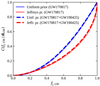 |
Fig. A.1. Cumulative posterior probability of the BNS jet incidence, showing the effect of adding GW190425 to the sample. The solid lines are the same as in Fig. 1 and account for GW170817 only, while the dashed ones account for GW190425 as well, as described in the text. |
Given this framework, a relevant question that can be addressed is how many secure identifications of a jet, and/or how many tight limits on its presence, are needed to constrain fj, GW to a desired precision. In that respect, we must keep in mind the fact that, while the presence of a jet can be assessed with relative certainty in favourable cases such as GW170817, its absence is generally much more difficult to prove, especially due to the strong relativistic beaming of radiation, which typically makes the detection of a putative jet extremely difficult beyond some limiting viewing angle. In well-localised cases, constraints from deep late-time radio observations can be used to probe a larger range of viewing angles, but for the majority of events this will not be a feasible route due to the combination of large localisation error box and low expected brightness of the late-time radio afterglow (e.g. Hotokezaka et al. 2016; Dobie et al. 2021; Colombo et al. 2022). This implies that it will be easier to constrain fj, GW from below than from above. With these considerations in mind, we performed a simple experiment: we assumed a true value fj, GW, true = 0.5 and constructed a sample of mock BNS events with jets assigned randomly with probability fj, GW, true. In order to represent in a simple way the jet detectability, for each event we randomly extracted a distance and an inclination from the universal joint distribution expected for GW-detected binaries (Schutz 2011). We then assumed a distance-dependent limiting viewing angle
![Mathematical equation: $$ \begin{aligned} \theta _{\rm v,lim}=\min \left[\frac{\pi }{2},\left(\frac{d_{\rm L}}{d_{\rm L,e}}\right)^{-2} \right] \end{aligned} $$](/articles/aa/full_html/2022/10/aa43260-22/aa43260-22-eq44.gif) (A.4)
(A.4)
beyond which observations are unable to constrain the presence, or absence, of a jet. Here dL, e is a parameter, which we set equal to the 25th percentile of the simulated distances, so that only for the closest 25 percent of the events a jet can be excluded with 100% confidence if not present. If, for the i-th binary, θv < θv, lim and a jet was present, then we set Ji = 1; in all other cases, we set Ji = 0. For all events, we computed Pmiss, i from Equations A.3 and A.4, therefore assuming that no detection can be made beyond θv, lim, no matter how extensive the observations.
Figure A.2 shows how the posterior probability on fj, GW evolves as we include an increasing number Nevents of these simulated events in the inference. The result suggests that several tens of detections are needed to be able to constrain the jet incidence to within 10-20%, and hundreds to get to a few percent constraint.
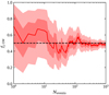 |
Fig. A.2. fj, GW inference with multiple GW-detected BNS mergers. The coloured bands show the evolution of the posterior 90% and 50% credible range on fj, GW after Nevents simulated GW detections (see text), while the red solid line shows the median of the posterior. The horizontal black dashed line shows the true value. |
Appendix B: Local rate density of GRB170817A-like sources
To estimate the local SGRB rate based on GRB170817A, we modelled the Fermi Gamma-ray Burst Monitor (GBM) detection of GRB170817A-like sources (i.e. sources with exactly the same luminosity and intrinsic gamma-ray spectrum as GRB170817A) as a Poisson process with an expected event number λ = R0VeffT over a time T = 13 yr (the current duration of the GBM survey), where Veff is the GBM effective sensitive volume. The posterior probability on R0, assuming a single detection, is
 (B.1)
(B.1)
where P(1 | R0)∝R0exp(−R0VeffT) and we adopted the Jeffreys prior  . We estimated the effective sensitive volume as
 (B.2)
(B.2)
where ηGBM = 0.59 accounts for the GBM field of view and duty cycle (Burns et al. 2016), dV/dz is the differential comoving volume (Hogg 1999), the (1 + z)−1 factor accounts for cosmological time dilation, and Pdet(z) represents the probability for GBM to detect a GRB170817A-like source at a redshift z within its field of view. In order to compute this quantity, we assumed, for simplicity, that the GBM detection probability only depends on the peak photon flux p64 of the GRB, measured with a 64 ms binning, in the 10-1000 keV band, so that Pdet(z) = Pdet(p64(z)). We then made the ansatz
![Mathematical equation: $$ \begin{aligned} P_{\rm det}(p_{64},\alpha ,p_{\frac{1}{2}}) = \frac{1}{2}\left\{ 1 + \tanh \left[\alpha \ln \left(\frac{p_{64}}{p_{\frac{1}{2}}}\right)\right]\right\} , \end{aligned} $$](/articles/aa/full_html/2022/10/aa43260-22/aa43260-22-eq48.gif) (B.3)
(B.3)
which is a smooth function satisfying Pdet = 1/2 when  , Pdet ∼ 1 when
  and Pdet ∼ 0 when
  . The α parameter controls the sharpness of the transition from 0 to 1. To fix α and
  , we proceed as follows. We assume the intrinsic inverse cumulative distribution of short GRB photon fluxes to follow
  , as expected for uniformly distributed sources in Euclidean space, in absence of evolution of the luminosity function with distance (which is reasonable as the typical redshifts are well below 1). The observed distribution is then
 (B.4)
(B.4)
We fit the resulting distribution to that constructed with the actual Fermi/GBM catalogue data (restricted to events with t90 ≤ 2 s) by minimising the sum of the squares of the residuals, obtaining α = 2.25 and  ph cm−2 s−1. The observed and modelled distributions are shown in Figure B.1.
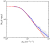 |
Fig. B.1. Fermi/GBM observed inverse cumulative distribution of 64-ms-binned photon fluxes in the 10-1000 keV band (blue solid line, with the grey band showing the 90% confidence band due to Poisson and measurement uncertainties), compared with our best-fitting model, Eq. B.4, with α = 2.25 and |


Given the GRB170817A measured (Goldstein et al. 2017) peak photon flux p64 = 3.7 ph cm−2 s−1, the best-fitting spectral model at the peak (second line of table 3 in Goldstein et al. 2017), the best-fitting host galaxy luminosity distance (Hjorth et al. 2017) dL = 41 Mpc, and assuming Planck cosmological parameters (Planck Collaboration XIII 2016), one can compute the 64 ms photon flux of an identical source at any redshift, p64(z). This allowed us to compute the integral in Eq. B.2, yielding Veff = 1.13 × 10⁵ Mpc3. Plugging this in Eq. B.1, we obtained the posterior probability distribution shown in Figure 2, whose peak and 90% credible interval are  Gpc−3 yr−1, in good agreement with the simpler estimate by Della Valle et al. (2018).
Appendix C: Comparison with GWTC-3
Figures C.1 and C.2 show comparisons of our mass distribution posteriors with the results from Abbott et al. (2021a) based on GWTC-3 (Abbott et al. 2021b) data. As a cautionary note, the definitions in our power law model match those of the POWER model from the GWTC-3 population study (Fig. C.1), but their PEAK model has the minimum mass cut Mmin as an additional free parameter (while ours is fixed at 1 M⊙). Despite being significantly shallower, our constraints are in general agreement with those from the population study.
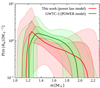 |
Fig. C.1. Comparison of our neutron star mass distribution posterior (power law model) with the GWTC-3 result from the population study described in Abbott et al. 2021a (their POWER model). Shaded areas show the 90% and 50% credible regions, while thick solid lines show the medians. Red is for our result (Sect. 4.2), blue is for the GWTC-3. |
All Figures
|
Fig. 1. Cumulative posterior probability of the BNS successful jet incidence. The solid red (blue) line refers to the fraction fj, GW of GW-detectable BNS mergers that produce a successful jet, based on having observed the single successful event GW170817 and adopting the Jeffreys (uniform) prior. The solid grey line refers to the jet incidence fj, tot in the entire BNS merger population, based on the ratio of the local rate of short GRB jets R0, SJ to the BNS rate R0, BNS. The implied 90% credible lower limits are annotated. |
| In the text | |
|
Fig. 2. Posterior probability distribution on the local rate density of GRB170817A-like events (grey solid line, Eq. (B.1)), SGRB jets in general (regardless of orientation, red solid line, Eq. (5)), and BNS mergers (as determined from observations of Galactic systems, blue solid line, Grunthal et al. 2021). |
| In the text | |
|
Fig. 3. Posterior distribution on the fraction fj, tot of BNS mergers accompanied by jets, computed as described in Sect. 2.2. The blue histogram shows the distribution of samples constructed as described in the text, that approximate Eq. (7), while the red line shows the analytical approximation |
| In the text | |
|
Fig. 4. Dependence of the disc mass on the mass of the secondary component in the binary, according to the fitting formula by Krüger & Foucart (2020). Different colours refer to different assumed equations of state, as shown in the legend. |
| In the text | |
|
Fig. 5. Merger remnant and GRB launching regions on the component mass plane. The filled coloured regions correspond to different BNS merger remnants on the (M1, M2) plane, assuming different EoSs: APR4 (left-hand panel), SFHo (central panel) and DD2 (right-hand panel). Grey hatches mark masses that are above the maximum non-rotating mass supported by the EoS. The black dashed lines enclose the region where our GRB jet-launching conditions are met, computed as described in Sect. 3.1 (the blue dashed lines, shown for comparison, are computed with the approximate method described in Sect. 3.3). White circles and contours show the best fit and 90% credible contours of masses of known Galactic BNS systems whose coalescence time tmerge is shorter than a Hubble time (tH, data from Farrow et al. 2019). The orange and green contours show the 50% and 90% credible regions for the component masses in GW170817 (Abbott et al. 2019) and GW190425 (Abbott et al. 2020a), respectively, adopting low-spin priors. |
| In the text | |
|
Fig. 6. Our prior on MTOV compared to recent model-dependent constraints in the literature. The blue thick line shows the marginalised MTOV prior we adopt in this work, which is constructed using the latest PSRJ0740+6620 mass measurement (Fonseca et al. 2021, grey filled area) as a lower limit and the remnant mass of GW170817 divided by 1.2 (pink filled area) as an upper limit (see text for an explanation). The remaining lines show results that combine multi-messenger constraints within different frameworks: the orange and green lines show the results obtained by Raaijmakers et al. (2021a) adopting their piecewise-polytropic (PP) and sound-speed (CS) parametrised EoS models, respectively; the dark red line shows the result from Legred et al. (2021) based on a non-parametric, Gaussian-processes-based EoS model; the purple line shows the result from Pang et al. (2021), who adopt an EoS model informed by chiral effective field theory. |
| In the text | |
|
Fig. 7. Probability that a BNS would satisfy our jet-launching conditions (Eq. (15)) as a function of the component masses M1 and M2, given our present knowledge of the EoS (encoded in the priors defined in Sect. 3.4). The masses of Galactic BNS systems that merge within a Hubble time and the two GW-detected BNS are shown for comparison, in the same way as in Fig. 5. |
| In the text | |
|
Fig. 8. Constraints on the parameters of a Gaussian BNS mass distribution model. Filled contours show the posterior probability density on the μm (mean) and σm (standard deviation) parameters of a Gaussian mass distribution model (assuming random pairing) obtained using fj = fj, GW, i.e. the constraint based on the association of GW170817 and GRB170817A (Sect. 2). Empty contours show the corresponding result for fj = fj, tot, i.e. the constraint based on the relative SGRB and BNS local rate densities (Sect. 2.2). The white star marks parameter values (μm, σm) = (1.33, 0.09) M⊙, representative of the main peak of the observed Galactic BNS mass distribution (Özel & Freire 2016). |
| In the text | |
|
Fig. 9. Constraints on the parameters of a power law BNS mass distribution model. Colours and lines have the same meaning as in Fig. 8. |
| In the text | |
|
Fig. 10. Mass distribution constraint. In each panel, filled contours show the 90% and 50% credible regions of the probability distribution P(m | θm) from which both M1 and M2 are sampled, while the thick solid line shows the median distribution at each m. The dj, GW constraint is used. Grey dashed lines show the edges of the corresponding 90% and 50% credible regions when using only the priors. Left-hand panel: the result for the power law mass distribution model, the central panel shows that for the Gaussian model, and the right-hand panel compares the two results with a log-scale vertical axis, to emphasise the lower 90% contour. |
| In the text | |
|
Fig. 11. Illustrative constraints on the EoS parameters assuming the power law mass distribution model with uniform priors on 1.1 ≤ Mmin/M⊙ ≤ 1.3 and −9 ≤ α ≤ 3.3, matching the 90% credible ranges of the GWTC-3 NS mass distribution constraint (Abbott et al. 2021a), and using a hypothetical future constraint on the jet incidence P(fj, GW | dGW)∝𝒩0.25, 0.05(fj, GW). |
| In the text | |
|
Fig. 12. Same as Fig. 11, but assuming a jet incidence constraint with a different mean, that is P(fj, GW | dtot)∝𝒩0.75, 0.05(fj, GW). |
| In the text | |
|
Fig. A.1. Cumulative posterior probability of the BNS jet incidence, showing the effect of adding GW190425 to the sample. The solid lines are the same as in Fig. 1 and account for GW170817 only, while the dashed ones account for GW190425 as well, as described in the text. |
| In the text | |
|
Fig. A.2. fj, GW inference with multiple GW-detected BNS mergers. The coloured bands show the evolution of the posterior 90% and 50% credible range on fj, GW after Nevents simulated GW detections (see text), while the red solid line shows the median of the posterior. The horizontal black dashed line shows the true value. |
| In the text | |
|
Fig. B.1. Fermi/GBM observed inverse cumulative distribution of 64-ms-binned photon fluxes in the 10-1000 keV band (blue solid line, with the grey band showing the 90% confidence band due to Poisson and measurement uncertainties), compared with our best-fitting model, Eq. B.4, with α = 2.25 and |
| In the text | |
|
Fig. C.1. Comparison of our neutron star mass distribution posterior (power law model) with the GWTC-3 result from the population study described in Abbott et al. 2021a (their POWER model). Shaded areas show the 90% and 50% credible regions, while thick solid lines show the medians. Red is for our result (Sect. 4.2), blue is for the GWTC-3. |
| In the text | |
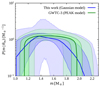 |
Fig. C.2. Same as Figure C.1, but for our Gaussian model and the GWTC-3 population study PEAK model. |
| In the text | |
Current usage metrics show cumulative count of Article Views (full-text article views including HTML views, PDF and ePub downloads, according to the available data) and Abstracts Views on Vision4Press platform.
Data correspond to usage on the plateform after 2015. The current usage metrics is available 48-96 hours after online publication and is updated daily on week days.
Initial download of the metrics may take a while.