| Issue |
A&A
Volume 697, May 2025
|
|
|---|---|---|
| Article Number | A20 | |
| Number of page(s) | 22 | |
| Section | Interstellar and circumstellar matter | |
| DOI | https://doi.org/10.1051/0004-6361/202245828 | |
| Published online | 30 April 2025 | |
Volume densities and star formation in nearby molecular clouds
1
IRAM,
300 rue de la Piscine,
38 406
Saint-Martin-d’Hères,
France
2
Chalmers University of Technology, Department of Space, Earth and Environment,
412 93
Göteborg,
Sweden
★ Corresponding author: This email address is being protected from spambots. You need JavaScript enabled to view it.
Received:
29
December
2022
Accepted:
2
December
2024
Abstract
Context. Volume density is a key physical quantity that controls the evolution of the interstellar medium (ISM) and star formation, but it cannot be accessed directly by observations of molecular clouds.
Aims. Our aim is to estimate the volume density distribution in nearby molecular clouds in order to measure the relation between column and volume densities and to determine their roles as predictors of star formation.
Methods. We developed an inverse modelling method to estimate the volume density distributions of molecular clouds. We applied this method to 24 nearby molecular clouds for which column densities had been derived using Herschel observations and for which star formation efficiencies (SFE) had been derived using observations with the Spitzer space telescope. We then compared the relationships of several column-density-based and volume-density-based descriptors of dense gas with the SFEs of the clouds.
Results. We derived volume density distributions for 24 nearby molecular clouds, which represents the most complete sample of such distributions to date. The relationship between column densities and peak volume densities in these clouds is a piecewise power law relation that changes its slope at a column density of 5–10 × 1022 H2 cm−3. We interpret this as a signature of hierarchical fragmentation in the dense ISM. We find that the volume-density-based dense gas fraction is the best predictor of star formation in the clouds, and in particular, it is as anticipated a better predictor than the column-density-based dense gas fraction. We also derived a volume density threshold density for star formation of 2 × 10⁴ H2 cm−3.
Key words: methods: statistical / stars: formation / ISM: clouds / ISM: structure
© The Authors 2025
 Open Access article, published by EDP Sciences, under the terms of the Creative Commons Attribution License (https://creativecommons.org/licenses/by/4.0), which permits unrestricted use, distribution, and reproduction in any medium, provided the original work is properly cited.
This article is published in open access under the Subscribe to Open model. This email address is being protected from spambots. You need JavaScript enabled to view it. to support open access publication.
1 Introduction
Volume density is one of the most important parameters affecting physical processes in the interstellar medium (ISM), from chemistry to thermodynamics, particle interactions, radiation mechanisms, and gas dynamics. Volume density is therefore a crucial parameter in any evolution model of the ISM, and consequently for any model of star formation.
Unfortunately, it is not possible to directly measure volume densities at the densities of typical star formation regions within molecular clouds (n(H2) ≳ 102 cm−3). Novel techniques that exploit Gaia data can infer the three-dimensional structure of the ISM using dust, but only at relatively low spatial resolutions (≳1 pc) and volume densities (≲1 H2 cm−3) that do not reach the actual birthplaces of stars (e.g. Green et al. 2019; Leike et al. 2020; Rezaei Kh. & Kainulainen 2022; Lallement et al. 2022). In contrast, at the densities intimately linked to star formation, we only have access to measurements of column densities. As a result, the detailed volume density structure of star-forming regions and its properties remain poorly known. This, in turn, hampers our understanding of the physics of ISM evolution and star formation.
When the geometry of the studied region can be assumed to be simple, such as a cylinder or a sphere, determining the volume density distribution can be done trivially via forward modelling (e.g. Alves et al. 2001; Kainulainen et al. 2016; Orkisz et al. 2019; Suri et al. 2019; Arzoumanian et al. 2019; Könyves et al. 2020). However, such assumptions are not generally applicable to the complex density structures of molecular clouds.
Similar approaches can be applied to galactic scales via assumptions about the gas geometry in the disk; a volumetric approach of star formation laws has proved to yield more robust correlation between gas and stars than the usual, surface-density-based approach (e.g. Bacchini et al. 2019a,b; Yim et al. 2022).
A number of more or less sophisticated inverse modelling approaches, that is methods that use the observed column densities to construct a model of the underlying volume densities, have been presented (e.g. Kainulainen et al. 2014; Krčo & Goldsmith 2016; Bron et al. 2018; Hasenberger & Alves 2020). One should also note the work of Xu et al. (2023), who combine the use of magnetohydrodynamic simulations and deep-learning techniques to predict mean volume densities of clouds based on the column density maps. Overall, however, the development of these methods is clearly still in progress, and none of the existing techniques has been systematically applied to major sets of observational data.
For this paper we made progress by developing a method that we call ‘from COLUMn to vOLUME’ (Colume) to estimate the volume density structure of molecular clouds. We then applied it to an extensive set of 24 molecular clouds observed with the Herschel satellite. This enabled us to present a new systematic study of the volume density statistics of molecular clouds, and specifically, the first one employing a complete set of the Herschel column density data available for nearby clouds. With the resulting density data in hand, we address whether star formation in the clouds is better traced by volume or column densities, and we also derive a volume density threshold for star formation.
The paper is organised as follows. In Sect. 2, we present in detail the principles and implementation of the Colume code, as well as the molecular cloud data to which we applied Colume and the star formation data that we confronted with our volume density estimations. Section 3 presents the obtained volume density estimations, as well as the observed correlations between column density, volume density, and star formation. The implications of these findings, as well as the possible caveats, are discussed in Sect. 4. Our findings are then summarised in Sect. 5. In Appendix A, we describe how we tested the Colume code on simulation data; in Appendix B we discuss the technical details of the implementation of Colume; and in Appendix C we discuss the impact of cloud anisotropy on the results.
2 Data and methods
2.1 Volume density estimation
In this section, we describe the principle of Colume, the volume density estimation algorithm that we implemented and applied to column density data of nearby molecular clouds. The code is publicly available. It has been implemented for the most part using NumPy (Harris et al. 2020) in Python3. The Colume code makes also extensive use of the scikit-image package (van der Walt et al. 2014) for image analysis (basic image processing, region identification and measurements), as well as the AstroPy package (Astropy Collaboration 2013, 2018) for astronomical data handling.
2.1.1 Basic principle and geometrical assumptions
Astronomical observations only give us access to the column density N (e.g. of gas, dust), which in the simplest case is a projection of the volume density field ρ in the plane of the sky,
 (1)
(1)
where z is along the line of sight. In the lack of knowledge about the three-dimensional structure of the volume density field subtending the column density map available to the observer, we have to make assumptions about what is deemed to be a probable geometry. In the case of the Colume code, the assumptions are as simple as possible and are the following:
The volume density structure is single-peaked along each line of sight.
The volume density structure is hierarchical.
Last but not least, it is necessary to estimate the dimension of volume density structures along the line of sight. The simplest and most common assumption here is that it is typically the same as the dimensions in the plane of the sky, and thus:
The volume density distribution is statistically isotropic.
 (2)
(2)
Here  is the area of an object in the plan of the sky, l is its depth along the line of sight and
  is its total volume. The factor α, of the order of 1, depends on the detailed geometry – for the sake of simplicity we have set α = 1, which strictly speaking is only valid for a face-on cube geometry (other options for α are discussed in Appendix C).
These assumptions allowed us to work with an incremental approach, where instead of considering the column density N and the volume density ρ directly, we rather describe them as sums of infinitesimal (or, in practice, finite) increments of density. In that way we can write for any line of sight (x, y) that
 (3)
(3)
The sampling ΔNi does not need actually to be regular (see Sect. 2.1.2 and Appendix B for a discussion).
Likewise, the volume density in all points of space would be defined as
 (4)
(4)
It is therefore these sums of Δρi(x, y, z) that we aim to reconstruct. However, we note that we do not claim to recover actual density profiles along the z direction, we only try to infer the statistical distribution of volume density for each line of sight.
In order to reconstruct the volume density increments, we consider the contour Ci associated with each column density increment ΔNi. Each such contour is considered as an individual, isotropic object, of area  , embedded in the contour Ci − 1 and itself providing a background for the contour Ci + 1. In three dimensions, this corresponds to volume density increments with associated volumes hierarchically nested within one another. The volume density increments Δρ are therefore defined as:
 (5)
(5)
Equation (5) implements the assumptions of our method, by setting the depth aspect ratio to α = 1, and ensuring that the volume density increment is not fragmented along the line of sight. Each volume density increment Δρi is then assumed to be fully embedded in the volume of the increment Δρi − 1 (where Ni > Ni−1). This excludes for example the possibility of an isolated dense clump in the diffuse foreground of a cloud.
An additional complexity comes from the fact that in practice the contours are not necessarily connected, but instead consist of several disconnected regions which need to be treated individually. Taking this into account makes the volume density estimation more computationally intensive, as it requires a topological analysis of each contour, but the cost is not prohibitive. The principle and assumptions of the computation remain exactly the same as described above, with the only difference that each sub-region  identified in a fragmented contour is treated in the way the entire Ci was treated before. This has the effect of giving to Eq. (5) an additional spatial dependence in addition to the value of N(x, y). Each sub-region
  now has a corresponding area
  , which implies:
 (6)
(6)
where  such that
  .
.
It should be noted that here, despite taking into account fragmentation of column density contours in the plane of the sky, we still assume that the identified regions correspond to connected volumes, meaning that there is no fragmentation along the line of sight.
From these, one can in particular compute the maximum volume density reached along each line of sight (hereafter peak volume density):
 (7)
(7)
The distribution (probability distribution function, PDF) of volume densities along each line of sight can also be described by the list of volume density values ρi(x, y), weighted by the corresponding depth along the line of sight li(x, y). The depth li(x, y) describes how much space along the line of sight is found at a volume density of ρi(x, y). For any value of ρi ≤ ρpeak(x, y), the quantities are simply obtained as:
 (8)
(8)
 (9)
(9)
Figure 1 illustrates the geometrical principle of the volume density estimation for a toy example in the disconnected case (taking into account plane-of-the-sky fragmentation). The column density map (here containing only three discrete levels) is decomposed into column density increments, and the area of the contours or sub-regions thereof is measured. The column density increments are then converted into volume density increments by attributing to them a depth along the line of sight, and the final density structure is reconstructed by summing the volume density increments. The resulting volume density estimation is represented in Fig. 1 as a three-dimensional rendering for illustration purposes only – the produced volume density data sets are instead maps of the volume density PDF for each line of sight. Such PDFs are shown for several lines of sight of our toy example in Fig. 2. In practice the depth li(x, y) can be converted to a volume vi(x, y) by multiplying it by the physical area of a resolution element (pixel) on the sky.
2.1.2 Practical implementation aspects
Defining column density increments requires a finite number of column density levels. The highest possible number of levels is dictated by the number of individual values found in the input data. With noisy data and a high-resolution quantisation, this can be as many as the number of pixels in the map – in such a case each contour is smaller than the previous one by only one pixel. The way volume densities are estimated by the Colume code requires having in memory the maps corresponding to all contours at the same time, which means X × Y × S data points, where X × Y are the native dimensions of the column density map, and S is the column density sampling, corresponding to the number of column density contours used. With the native (i.e. maximum) number of levels, this means effectively close to (X × Y)2 data points, which leads to unmanageable computations in terms of random-access memory requirements, even for fields of moderate sizes. It is therefore crucial to reduce the data complexity by sampling the column density distribution in an efficient way, that is in a way that recovers as much as possible of the detailed cloud structure while using as few column density levels as possible.
The choice of the sampling method depends among other things on the range of the column density distribution that need to be described most accurately. In this work, we have used the same sampling for all the studied column density maps. The sampling method is based on the column density percentiles (which ensures that there are no empty bins), with 2000 bins and an inverse logarithmic (i-log) spacing. The i-log spacing is the logarithm of a linear spacing, scaled to the range of the data (or, in that case, from 0 to 100 as we are considering percentiles). This sampling method and other possible sampling choices are discussed in Appendix B. At this stage the data is compressed by posterisation: in each bin, the individual column density values are replaced by the average value within the bin. In the column density map, this effectively creates contours, which are then used to compute areas and volumes as described in Sect. 2.1.1.
Once all the depths along the line of sight and all volume density increments have been computed, the yielded data structure is made of two three-dimensional arrays: a map of the lists of volume densities for each line of sight, and a map of the lists of associated volumes (physical area of a pixel × depth along the line of sight) – which can together be described as a map of weighted volume density PDFs as described in Eq. (9). The dimension of these arrays is X × Y × S. If the column density is very finely sampled, the resulting arrays are therefore not only very large, but also very sparse, since only the one point with the highest column density value is enclosed in all the contours and is therefore described to the highest complexity level – each line of sight is described by as only many volume density levels as the number of contours it was enclosed in. A compromise between saving two impractically large file or an impractically high number of small files (two per line of sight) is to save the computation results on a row-per-row basis in individual, two-dimensional NumPy-array files. A folder with 2X + 1 files is therefore generated – the additional file being a copy of the header of the input column density map.
In addition to the comprehensive data structure described above, there is the possibility to extract only the basic information about the volume density in the cloud, namely the peak volume density, and the global volume density PDF (i.e. the sum of the PDFs of all the lines of sight). This data format is a highly lossy compression, but it is also much lighter and easier to handle, as it only produces a two-dimensional map and a one-dimensional PDF, instead of two large three-dimensional data-cubes. It also offers the advantage of portability, since the map of peak volume densities can be saved in the FITS format, and the global PDF as a text file. Incidentally, this was also the data format used for the present study. This data format is illustrated in Fig. 3.
Regarding the different geometrical treatments described in Sect. 2.1.1, both the connected and disconnected treatment of contours are implemented in Colume. While the disconnected estimator offers a more detailed treatment of the column density morphology, and is physically more realistic, the connected estimator has the interesting property of being a lower limit estimator for the peak volume densities. This is due to the fact that the column density increments are ascribed to the largest reasonably possible volume (i.e. a connected, isotropic blob), whereas any modification (fragmentation, anisotropy) would tend to reduce this volume and therefore increase the volume density. Because all the lines of sight within a given column density contour are considered to belong to the same volume, it also produces a one-to-one correspondence between column and volume density values. In this work however, since we focus on star formation and therefore need accurate volume densities of dense gas in highly fragmented contours, we used exclusively the disconnected estimator.
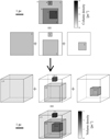 |
Fig. 1 Schematic representation of the volume density estimation. The indicated numbers correspond to the column (respectively volume) density values, in arbitrary units. Top half: original column density map with contours that define the following structures: a 9 pc2 diffuse background a, a main cloud with a 4 pc2 intermediate density envelope b and a 1 pc2 dense core c, and a small isolated 0.25 pc2 dense clump d. The column density map is then decomposed into column density increments. Bottom half: column density increments are converted into volume density increments by ascribing to them depths equal to the square root of their area (3 pc, 2 pc, 1 pc and 0.5 pc for the diffuse background, the envelope, the core, and the clump, respectively). The final volume density structure is obtained by summing the volume density increments, assuming that each successive increment is nested within the volume underlying the previous contour. The nested volumes are represented in the mid-plane along the line of sight only by convention. |
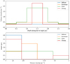 |
Fig. 2 Different representations of the volume densities reconstructed for the simple example illustrated in Fig. 1. Top: density profile along lines of sight corresponding to the different environments in the map (diffuse background, intermediate density envelope, dense core, small isolated clump). The nested dense structures are represented in the mid-plane along the line of sight only by convention. Bottom: PDFs of volume densities along the line of sight corresponding to the above lines of sight. The densities are expressed in the same arbitrary units as in Fig. 1. The statistical weights are equivalent to depths along the line of sight, as represented in the top panel. |
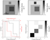 |
Fig. 3 Main products of the Colume volume density estimation (similar to Fig. 4) obtained for the simple example illustrated in Fig. 1. Top left: original column density data. Top right: peak volume density reached along each line of sight. Bottom left: comparison of the column density (black) and volume density (red) histograms for the entire area (respectively volume) of the cloud. Bottom right: joint distribution of the column density and peak volume density. |
2.1.3 Method validation
In order to check whether the volume densities obtained with Colume are reasonably close to the truth, we tested the reconstruction in a case were the 3D information is known, namely on numerical simulations. The tests were run on a 4 × 10³ M⊙ cloud in a 40 × 40 × 40 pc cube, their results are described in detail in Appendix A.
We have in particular checked the quality of the reconstructed peak and mean volume densities along the line of sight, and of the global volume density PDF, for projections along all three axes of the simulated cube, in both a noiseless and noisy case. The tests have in particular highlighted the reliability of the volume density PDF and the robustness of our isotropy assumption, since the reconstructed PDFs are very consistent from one projection to the other and show little sensitivity to noise.
While the average volume densities are very well reproduced, a systematic non-uniform bias is observed in the reconstruction of the peak volume densities. While the values are well reconstructed for low (∼100 cm−3) and high (≳104 cm−3) peak column densities, at intermediate values the peak volume density can be underestimated by as much as an order of magnitude. This is interpreted as being due to the fact that for the lowest and highest volume densities, we are dealing with the envelope of the cloud or dense cores respectively, which both comply well with the isotropy assumption, whereas between these cases the gas is structured into sheets and filaments which have high aspect ratios, their volumes thus get overestimated and densities consequently underestimated.
We also show that on average volume densities tend to get slightly biased towards higher values in the presence of noise, because the contours of the column density increments tend to get fragmented by the noise, which leads to smaller areas, thus smaller reconstructed volumes and higher densities. This effect is however moderate in comparison with the other uncertainties of the method, and is largely negligible with high signal-to-noise ratio data.
2.2 Molecular cloud sample
In order to show the potential of Colume volume density estimations in the study of ISM and star formation with observational astronomical data, we applied it to a sample of molecular clouds for which homogeneous and high-quality column density maps as well as young stellar object (YSO) catalogues are available. The chosen cloud sample and the corresponding column density maps and YSO catalogues are described in the following sections.
2.2.1 Column density maps
In order to benefit from the best possible conditions to run Colume, we needed a sample of column density maps with a high signal-to-noise ratio, a high spatial resolution, a homogeneous data reduction, and a wide diversity of environments. These requirements led us to choose the column density maps published for the set of 25 dense clouds observed by the Herschel Gould Belt Survey (HGBS, André et al. 2010). These nearby clouds have masses ranging from 16 M⊙ to 89 × 103 M⊙, with very different levels of star formation activity.
The studied clouds, as published by the HGBS consortium, are the following: the Aquila Rift (W40) cloud complex (Bontemps et al. 2010; Könyves et al. 2015), the Cepheus Flare clouds (Di Francesco et al. 2020), the Chamaeleon cloud complex (Winston et al. 2012; Kóspál et al. 2012; Alves de Oliveira et al. 2014), the Corona Australis cloud (Sicilia-Aguilar et al. 2014; Bresnahan et al. 2018), IC5146 (Arzoumanian et al. 2011, 2019), the Lupus cloud complex (Rygl et al. 2013; Benedettini et al. 2018), the Musca cloud (Cox et al. 2016), the Ophiuchus L1688 and L1689B clouds (Roy et al. 2014; Arzoumanian et al. 2019; Ladjelate et al. 2020), the Orion A (Roy et al. 2013; Polychroni et al. 2013) and Orion B (Schneider et al. 2013; Könyves et al. 2020) giant molecular clouds, the Perseus cloud (Pezzuto et al. 2012, 2021; Sadavoy et al. 2012, 2014), the Pipe nebula and B68 (LDN 57) globule (Peretto et al. 2012; Roy et al. 2014), the Polaris Flare (Men’shchikov et al. 2010;
Ward-Thompson et al. 2010; Miville-Deschênes et al. 2010), the Serpens (Serpens Main + Aquila East) cloud complex (Fiorellino et al. 2021), and the Taurus molecular cloud (Palmeirim et al. 2013; Kirk et al. 2013; Marsh et al. 2016).
In summary, the column density maps were obtained from the observational data in the following way (see the above-cited HGBS papers for details). The Herschel observations were carried out in parallel in all the bands of the SPIRE (Spectral and Photometric Imaging Receiver) and PACS (Photodetector Array Camera and Spectrometer) instruments. After data reduction, zero-level offsets were adjusted using Planck data. The spectral energy distributions (SED) thus obtained were then fitted on a pixel-by-pixel basis with a modified black-body, with a dust opacity law of κλ = 0.1 ×(λ/300 μm)β cm2 g−1 and a dust emissivity index β = 2 (Hildebrand 1983), which produces column density and effective dust temperature for the entirety of the observed maps. The produced maps are expressed in H2 cm−2, taking only into account the hydrogen contribution to the column density, without helium and metals.
The maps provided by the HGBS consortium1 were reprocessed before the Colume processing. Given that the volume density computations are very memory-intensive, it was crucial to reduce the size of the files to a minimum. For this purpose, the maps were rotated depending on the shape of the observed field, in a way which allowed cropping as much blank area as possible. The maps were also resampled to a homogeneous 12″ pixel size – a sufficient sampling given the typical beam size of 36.3″, but which allows for much smaller files than the original 3″ sampling. To account for artefacts caused by the resampling as well as to remove noisy pixels at the edges of the observed field, the maps were submitted to 3 iterations of binary erosion (i.e. their blanking mask was dilated 3 times), which corresponds to a full beam width. The column density values below 1 × 10²⁰ H2 cm−2 were then blanked out, since several maps featured spurious values below this threshold, and column densities below this value are anyway largely irrelevant for star formation on the studied scales. After this blanking step, the maps were eroded once more to smooth out the effect of the thresholding.
The reframing applied in several HGBS papers to remove the noisy edges of the maps was not implemented, since it was largely redundant with the filtering described above.
2.2.2 Distances to the clouds
For each cloud, the distance was adopted based on the catalogue created by Zucker et al. (2020), which provides distances to the first major extinction jump along the line of sight, which corresponds to the close end of the dense cloud. Since it often happens that many lines of sight of the Zucker et al. (2020) catalogue fall within a given Herschel field, we adopted as our reference distance the line of sight closest to the centre of projection of each field. In the case of the Perseus cloud, the centre of projection happens to coincide with a ‘hole’ in the cloud, where the estimated distance is the furthest of all available lines of sight, about 20% further than the average – we therefore used in that case the average distance of all the lines of sight corresponding to the field. The variation in distance from one line of sight to the other within a field is generally of the order of ∼10% (when applicable), which in turns reflects as 10% of uncertainty on the volume densities (via the uncertainty on the depth along the line of sight which is directly proportional to the distance).
The only exception to this distance procedure is the B68 globule, which, in the absence of foreground stars, lacks a relevant line of sight in Zucker et al. (2020) – the line of sight closest to the centre of projection of the B68 field is the same as for the Pipe Nebula. The distance to B68 was thus set based on the most recent available distance measurement, from de Geus et al. (1989).
2.3 YSO samples and star formation properties
A homogeneous catalogue of YSOs was not available for the entire sample of clouds in our study. We therefore had to aggregate data from several YSO surveys. To select these surveys, rather than choosing the most recent (and arguably most complete) ones, we decided to focus on obtaining a catalogue which would be as homogeneous as possible in terms of sensitivity and methodology, and therefore completeness. This implied to have observations and data reduction carried out in similar ways, and having access to detailed YSO catalogues, rather than YSO counts, to enable cross-checking.
For almost all the clouds in our sample, the YSO data was obtained from the catalogue created by Dunham et al. (2015), which compiles a large YSO catalogue based on the legacy data of the c2d (Evans et al. 2003) and Gould’s Belt (Gutermuth et al. 2009) surveys. We complemented this with several other catalogues: for the Orion clouds (Orion A and Orion B), we used the study of Megeath et al. (2012); for the Pipe nebula and the B68 globule, we used the data of Forbrich et al. (2009); for the Taurus cloud, we used results from Rebull et al. (2010). Finally, not a single YSO is known to be present in the Polaris Flare (Ward-Thompson et al. 2010; André et al. 2010).
The main properties of each of these YSO catalogues are nearly identical. All studies are based on multi-band observations made with the MIPS (Multiband Imaging Photometer for Spitzer, Rieke et al. 2004) and IRAC (InfraRed Array Camera, Fazio et al. 2004) instruments of the Spitzer space observatory. The data reduction follows standard Spitzer pipelines, and the extracted point sources are matched with the Two-Millimetre All-Sky Survey (2MASS, Skrutskie et al. 2006) catalogue. The identification of YSOs is then in all cases performed using a combination of colour-colour diagrams (or spectral indices) and colour-magnitude diagrams across the MIPS and IRAC bands, although the details of the choice of diagrams optimal for this identification varies from study to study. The main difference between the YSO samples is the quality assessment of the YSO candidates performed by Rebull et al. (2010): after a first selection made using exclusively Spitzer and 2MASS data, the reliability of the YSO candidates was examined using additional observational data from the Canada-France-Hawaii Telescope (CFHT) and Sloan Digital Sky Survey (SDSS) in the optical, as well as XMM-Newton in the X-ray and ultraviolet. To a lesser extent, the approach taken in Megeath et al. (2012) is also different from the rest of the sample in the way that completeness and contamination of the YSO sample are tested statistically using artificial stars and comparison with reference fields. However, overall the discrepancies between the assembled YSO catalogues are minor, and for lack of a single, uniform YSO catalogue of all nearby molecular clouds, they still constitute for our sample of clouds the best possible database for the study of star formation properties in terms of self-consistency and data quality.
For each catalogue, we checked the positions of the YSOs against the spatial coverage of the corresponding column density maps. The YSOs were then selected according to their spectral type, namely class 0, class I, flat-spectrum and class II, either using directly the spectral classification provided in the catalogues (Forbrich et al. 2009; Megeath et al. 2012; Rebull et al. 2010), or inferring the class from the spectral measurements (Dunham et al. 2015). Only the robustly identified YSOs were retained, which implies removing from the sample sources identified as likely asymptotic giant branch (AGB) stars (Dunham et al. 2015), removing rejected candidates (Forbrich et al. 2009), keeping only candidates with the highest confidence levels (‘new member’ or ‘probable new member’ only, Rebull et al. 2010). In the case of Orion A and Orion B, Megeath et al. (2012) estimate a residual contamination of 6.1 per deg2 from extragalactic sources, and that a further 13 sources are likely misidentified as YSOs, we therefore subtracted these contaminants from the total YSO count in each field by multiplying 6.1 by the field area and attributing the remaining 13 sources based on the prorata of YSOs identified in Orion A and Orion B – this leads to non-integer YSO numbers in these two clouds.
The star formation rate (SFR) and star formation efficiency (SFE) of the clouds are then derived as
 (10)
(10)
where NYSO is the YSO count for each cloud, MYSO = 0.5 M⊙ is the average YSO mass (Chabrier 2003), τYSO = 2 Myr is the average YSO lifetime (Evans et al. 2009), and Mcloud is the cloud mass, obtained by integrating the column density maps above a threshold of 1.105 × 10²¹ H2 cm−2 (see Sect. 3.2.1 for details).
The star formation properties for each cloud are summarised in Table 1. The YSO positions for all clouds are plotted in the supplementary online material (YSO_all).
3 Results
3.1 Volume densities in nearby molecular clouds
3.1.1 Volume density distributions
We applied Colume to the entire sample of 25 clouds. The reconstructed volume densities range from 1.3 H2 cm−3 in the diffuse background of Orion A, to 1.3 × 10⁶ H2 cm−3 in the densest core identified in Oph L1688. The lowest reconstructed volume densities depend both on the (low) column densities in a given field and on the total area of the field (and hence the reconstructed maximum depth along the line of sight); it is thus no surprise to find the lowest reconstructed density in the second largest map in our sample. We also note the presence of values higher than 1.3 × 10⁶ H2 cm−3 in the Lupus clouds, but these are single-pixel noisy values at the edges of the maps, whereas the dense cores in Oph L1688 are robust structures, observed with a high signal-to-noise ratio and displaying a reliable morphology. All gas densities are expressed in units of H2 to be consistent with the (dust-derived) HGBS data sets, but at the lowest column and volume densities one should note that not all hydrogen is expected to be present in the form of H2; however, the H/H2 fractionation is beyond the scope of this paper.
For the purpose of this pilot study, we only used the compressed version of the results, that is, the peak volume density maps and the global volume density PDFs. An example of these results is presented and compared with the original column density data in Fig. 4 for the case of the Cep1228 cloud – the rest of the cloud sample is presented in the supplementary online material.
Common features emerge when comparing the volume density with column density in these figures. The maps of peak volume density (maximum volume density along the line of sight) show the concentrations of gas fragmented into a number of cores, and these cores are immersed in a common low-density envelope. In addition to this pattern, and at almost all densities (but most visible at the lowest densities), one can see the presence of small high-density clumps. While it is tempting to attribute these clumps to noisy fluctuations of the column density maps, their aspect is different from the effect of added noise observed when testing Colume on simulations (Figs. A.4 and A.5), it is therefore likely that they reflect the real, clumpy structure of the ISM at all densities. The features of the column density PDFs (secondary peaks, slope breaks...) are for the most part reproduced in the volume density PDFs, but often appear smoothed out. A general exception can be noted regarding features at column densities lower than the main peak of the PDF, which are not found in volume density; this is most likely a sampling effect. The tail of the volume density PDFs is in general flatter and longer than the one of column density PDFs, which corresponds to a larger dynamic range in volume than in column densities (see Sect. 4.2).
Cloud sample and basic properties collected or directly derived from the literature.
3.1.2 Correlation of peak volume density with column density
The joint distribution of the column and peak volume density (Fig. 4, lower right) presents a characteristic shape for all the clouds, which can be described as feather-like. A very tight correlation is found in a main ‘stem’, which acts as a lower limit for the peak volume density for any column density, and extends throughout the entire data range. Above a certain volume density, the ‘barbs’ start to branch off from the stem; each of these barbs also traces a very tight correlation, some of which can branch again later. In the end, the cloud of points which represents the joint histogram of peak volume density versus column density for the entire cloud is actually the sum of a large number of line-like correlations of various statistical weights which get superimposed on each other.
This structure arises from the hierarchical reconstruction of the volume density. Each line-like correlation corresponds to a single region containing nested column density contours. As long as the successive contours are connected, they yield a single value of area, thus depth, and therefore a one-to-one correspondence between column density and volume density. But as soon as a contour break into two or more sub-regions, the one-to-one correspondence is lost and the correlation branches off. In this context, the main stem corresponds to the largest sub-region for each column density contour, it thus ranges from the contour enclosing the entire field to the contour containing the highest column density value in the map. This behaviour for example is very clear in the case of a small field with a very simple morphology such as the B68 globule (supplementary online material, B68).
The relation between column density and peak volume density is particularly interesting as it allows in principle to use the column density to infer the highest volume densities reached along any line of sight – these highest densities being the ones involved in star formation. We therefore tried to characterise the average relation between column and peak volume density for the entire cloud sample. The joint distribution of column densities and peak volume densities for all the fields combined is shown in Fig. 5.
The main stems of the joint distributions of the individual clouds come out clearly as bright lines almost parallel to each other at low densities. A group high volume density points draws the eye in the shape of the distribution, but these are negligible in terms of statistical weight and correspond to noisy pixels at the edge of some of the column density maps. What is more significant is the lower edge of the distribution, which shows a change of slope around 5–10 × 1021 H2 cm−2. Given that the majority of the data points are close to this lower edge, we have tested if the overall correlation reflects this change of slope. We therefore fitted this correlation with a power law, over the entire data range, and in two limited column density ranges, corresponding to the commonly used definition of low-density and high-density molecular gas (see Sect. 3.2.1, namely AV = 1–8 mag and AV > 8 mag – in our case converted to N = 1.11 × 10²¹–8.84 × 10²¹ H2 cm−2 and i > 8.84 × 10²¹ H2 cm−2 using the conversion factor NH/AV = 2.21 × 10²¹[cm−2/mag] (Güver & Özel 2009); the threshold set at AV = 8 mag corresponds visually to the location of the change of slope. The results of the fitting are visualised in Fig. 5 and detailed in Table 2. The very small errors in the fit results do not indicate a tight correlation – the measured root mean square (RMS) scatter is indeed large – but merely that the fit is well-constrained by the very large number of data points.
Properties of the correlation between column density and peak volume density in the Gould Belt for different density ranges.
The fit of the entire density range is dominated by the low- to intermediate-density material, which vastly dominates the cumulative area of the studied sample of clouds. On the other hand, the change of slope is well visible in the power-law exponents of the two-part fit, with a low-density exponent of ∼0.9 and a high-density exponent of ∼2.2. This suggests a difference in physical conditions, or at least in cloud morphology, between the two density regimes, and is further discussed in Sect. 4.2.
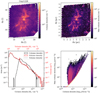 |
Fig. 4 Main products of the Colume volume density estimation for the Cep 1228 molecular cloud. The same figures for all clouds in our sample are shown in the supplementary online material. Top left: column density map obtained from HGBS data, the arrow indicates north. Top right: map of the peak volume density (maximum volume density reached along a line of sight). Bottom left: comparison of the column density PDF (solid black) and reconstructed volume density PDF (solid red) for the entire cloud. The dash-dotted line corresponds to the smoothed volume density PDF used to determine the volume density contrast. The data ranges are different, but the scaling is the same for the column and volume density case. Bottom right: joint distribution of the column density and peak volume density for each line of sight. |
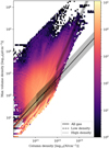 |
Fig. 5 Joint distribution of the column density and peak volume density, for all the lines of sight of all the clouds in the sample. The trend of this distribution has been fitted as a power law in three column density regimes: for the entire column density range present in the data (solid line), for the low-density molecular gas defined as AV = 1–8 mag (dashed line), and for the dense gas defined as AV > 8 mag (dotted line). The RMS scatter around the best fit relation is represented by the shaded areas. |
3.2 Star formation versus column and volume density
3.2.1 Measuring the dense gas
Star formation requires dense gas to proceed, but it is necessary to quantify how this dense gas is defined, and whether the density requirement is absolute (gas above a certain density threshold can contribute to star formation; e.g. Gao & Solomon 2004; Lada et al. 2010), or relative (only a top fraction of the gas in clouds can contribute to star formation, independent from the mean density of the parent cloud; e.g. Kruijssen et al. 2014; Spilker et al. 2021, see Padoan et al. 2014 for a review). We therefore used two different metrics to empirically describe the density distribution in the studied clouds – the dense gas fraction and the density contrast – and applied them to both the column density PDF and the volume density PDF of each cloud.
The dense gas fraction, initially introduced by Lada et al. (2010), is a commonly used descriptor of the amount of gas effectively involved in the star formation process via gravitational collapse. The dense gas fraction is defined as the ratio of the mass of the dense gas to the mass of the bulk of the cloud. The density contrast, introduced by Spilker et al. (2021), provides instead a relative measure of the gas density, based on the properties of the individual column density PDFs rather than on predefined thresholds. This density contrast is defined between a low density corresponding to the peak of the density PDF, and a high density above which 5 per cent of the mass of the cloud resides (this mass being considered only above the low-density limit). Both these descriptors also present the advantage of not relying on a model of the PDF shape (e.g. a power-law or a log-normal distribution), which would not necessarily fit the data well (Spilker et al. 2021).
In practice we adopted the following definition for the column-density-based and volume-density-based dense gas fraction ( and
and  ) and density contrast (ΔN and Δρ):
 (11)
(11)
where for all clouds the thresholds are Ncloud = 1.11 × 10²¹ − 8.84 × 10²¹ H2 cm−2 and Ndense = 8.84 × 10²¹ H2 cm−2, based on the commonly used extinction thresholds AV = 1 mag and AV = 8 mag (Lada et al. 2010; Kainulainen et al. 2013; Evans et al. 2014; Spilker et al. 2021), and with a conversion factor of NH/AV = 2.21 × 10²¹[cm−2/mag] (Güver & Özel 2009); similarly, we have
 (12)
(12)
where for all clouds the thresholds are ρcloud = 2 × 10² H2 cm−3 and ρdense = 2 × 10⁴ H2 cm−3, based on the results of tests described in more details in Sect. 3.2.2 following and approach similar to what Lada et al. (2010) used to derive the column density thresholds;
 (13)
(13)
where Npeak and ρpeak are respectively the column density and the volume density values corresponding to the peak (most probable value) of their respective PDFs, and the top 5% values N5% and ρ% are defined by:
 (14)
(14)
Dense gas measurements for all the clouds in the sample.
The determination of the value of Npeak and ρpeak from a PDF which is in practice a discrete histogram is very sensitive to sampling, which can change the limits of bins and thus affect the number of points in each bin. To alleviate this effect, we used a constant number of bins for all the column and volume density histograms (100 bins with logarithmic sampling), and we also smoothed the obtained histograms with a 3-bin wide sliding average (Fig. 4, lower left). The peak value used as Npeak (or ρpeak respectively) was then extracted from these smoothed histograms. The values of  , and Δρ for all the clouds in our sample are presented in Table 3.
We compared them for each cloud with the star formation efficiency (Eq. (10)) derived from the YSO counts described in Sect. 2.3. The choice of the SFE rather than SFR allowed for a better comparison between the clouds, given than the SFE is, like all the dense gas descriptors, normalised by cloud mass. The correlations between the SFE and  or Δρ were then quantified by performing a fitting. The fitting was linear in each case, and was performed in log-log space in the case of SFE versus
  and
and  , and in lin-log space in the case of SFE versus ΔN and Δρ, since the density contrast is already defined as a logarithmic quantity. Considering the star formation efficiency in log space also effectively excluded from the correlation the B68, Cep1241 and Polaris fields, the SFE of which is 0. The tightness of the correlation was in each case estimated both in terms of the fit quality (R2, or error on the fit parameters), and it terms of RMS scatter with respect to the fitted linear relation. These correlations and the fitting results are presented in Fig. 6 and in Table 4. The narrowest scatter was obtained for the column-density-based density contrast (0.189 dex), while the volume-density-based dense gas fraction not only yielded a RMS scatter almost as tight as the best one (0.197 dex), but had also by far the best fit, making it overall the best available predictor of star formation.
Fitting results of the correlation between SFE and the different dense gas descriptors.
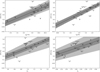 |
Fig. 6 Correlation of SFE with various metrics of the dense gas component in clouds. In each case a power law is fitted (solid line), the fit errors are represented in light grey, and the (Gaussian) spread of the cloud of points with respect to the fitted line is represented in dark grey. Top left: SFE vs. column-density-based dense gas fraction. Top right: SFE vs. volume-density-based dense gas fraction. Bottom left: SFE vs. column-density-based density contrast. Bottom right: SFE vs. volume-density-based density contrast. |
3.2.2 Volume density threshold for star formation
Translating the column-density-based definition of the density contrast ΔN to volume densities is straightforward (owing to the data-based nature of this descriptor). Adapting the definition of the dense gas fraction fdg for the volume density case, however, requires defining appropriate low- and high-density thresholds. Based on our sample and following an approach close to the one initiated by Lada et al. (2010), we obtained values of 2 × 10² H2 cm−3 and 2 × 10⁴ H2 cm−3 low- and high-density thresholds, respectively, which mirror the AV = 1 mag and AV = 8 mag extinction thresholds used in the column density case.
The high-density threshold corresponds to the density above which the gas reservoir is the most directly involved in star formation. This was quantified by Lada et al. (2010, their Fig. 3) by measuring the correlation between the number of YSOs in a sample of clouds, and the mass of gas above a given density threshold. The tightest correlation was found for a threshold of AK = 0.8 ± 0.2 mag, corresponding to AV = 7.3 ± 1.8 mag.
The low-density threshold is used to separate the bulk of the molecular cloud from its diffuse fore- and background. This enables normalising the relation between star formation and gas reservoir by the cloud mass, which becomes a relations between SFE and dense gas fraction, and therefore makes it possible to compare clouds of different sizes. The commonly used value of AV = 1 mag stems from the AK = 0.1 mag threshold introduced for that purpose by Lada et al. (2012), it is also close to the extinction levels at which molecular (12CO) emission starts to be detected (e.g. Goldsmith et al. 2008; Pety et al. 2017; Lewis et al. 2021).
For volume density thresholds, we assumed in practice that the low-density threshold should be approximately the volume density at which the gas becomes molecular, so of the order of ∼ 100 H2 cm−3 (Heyer & Dame 2015; Pety et al. 2017). The high-density threshold, on the other hand, could in principle be anywhere between the density at which the gas typically gets structured into a filamentary network (∼1 × 10³ H2 cm−3, Pineda et al. 2010; Orkisz et al. 2019), and the densities reached in prestellar cores (5 × 10⁴−1 × 10⁶ H2 cm−3, e.g. Evans et al. 2009; Teixeira et al. 2016). We therefore tested a range a value for both the low-density threshold (1 × 101−5 × 10² H2 cm−3) and the high-density threshold (1 × 10³−1 × 10⁶ H2 cm−3). The resulting scatter in the correlation between  and SFE is presented in Fig. 7.
One can observe that varying the low-density threshold has a minor effect on the tightness of the correlation, as shown by the fluctuation in position of the transparent blue plots in Fig. 7. The main variation comes from the value of the high-density threshold, and the minimum scatter is obtained at (or very close to) the same value of high-density threshold, namely 2 × 10⁴ H2 cm−3, for all values of low-density threshold. The high-density threshold of 2 × 10⁴ H2 cm−3 is therefore a robust result in terms of producing the smallest scatter in the correlation between  and SFE. The absolute minimum scatter is obtained with a low-density threshold set at 2 × 10² H2 cm−3.
We also note that scatter values for high-density thresholds beyond 5 × 10⁴ H2 cm−3 (shaded area in Fig. 7) are not meaningful, because several clouds in our sample do not reach such high volume density values, while still exhibiting star formation. Higher density thresholds for star formation not only produce poorer correlation measurements due to the diminishing number of clouds in the sample, but would also be in contradiction with the presence of active star formation in the clouds not reaching these densities.
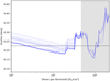 |
Fig. 7 Determination of the volume density thresholds yielding the tightest correlation between the volume density and star formation. Each transparent blue line corresponds to a different value of the low-density threshold between 10 H2 cm−3 and 5 × 10² H2 cm−3, the solid blue plot corresponds to the optimal threshold of 2 × 10² H2 cm−3. The dashed horizontal line at 0.225 dex corresponds to the spread obtained when using column densities. Values for a dense gas threshold higher than 5 × 10⁴ H2 cm−3 (shaded area) are not considered because not all clouds in the sample reach such high values and the statistics thus become less and less reliable. |
4 Discussion
4.1 Overview of limitations
The quality of our results is subject to two independent sets of limitations, one coming from the data used, and the other from our data processing, which means the Colume algorithm and the way it is applied to the data.
Regarding the data used, we made the choice to favour homogeneity over quality. As explained in Sect. 2.3, the YSO catalogues that we used are not the most recent and arguably most complete available. This has implications in terms of completeness and reliability of the YSO sample – for example, the YSO catalogue for the Orion complex produced by Megeath et al. (2016) using additional Chandra X-ray data contains 408 more YSOs than the (Megeath et al. 2012) catalogue that we used, and including completeness corrections it is estimated that the Orion complex contains a total of 5104 YSOs, rather than the 3481 we used as a starting point. However, while incomplete YSO catalogue do affect the measurements of star formation rates, the overall scaling between star formation and dense gas should not be affected significantly: the homogeneity of the YSO catalogues ensures that the completeness fractions should be approximately the same for all clouds, and therefore the slopes of the correlations we measured should be unchanged.
The column density data used pose another question. While extremely homogeneous in terms of observations and data reduction, given that all the maps were obtained in the same observational survey, the column density maps are arguably not the best possible that could have been obtained using the Herschel data. Other, more refined ways of computing total column densities from SEDs than pixel-by-pixel modified black-body fitting do exist, like for example the PPMAP (Marsh et al. 2016) method. In addition, the column density values obtained by the HGBS consortium from their observational data do not necessarily agree with other estimations of column density for the same clouds, obtained either from other observations (notably extinction data) or even using the same Herschel data, as can for example be seen in Könyves et al. (2020) and Lombardi et al. (2014). Re-deriving column densities is beyond the scope of this study, hence our use of the published data as they are. While the homogeneity of the column density data set ensures that the measured correlations with volume densities and with star formation properties remain valid, absolute values such as the volume density threshold for dense gas could be shifted if a different derivation of column densities had been used.
The selection of fields to be passed to Colume also raises questions, on two particular points: noise, and completeness.
The question of noise was also faced by the HGBS team when studying these clouds, and is mostly restricted to the edges of certain maps (Cepheus Flare and Lupus in particular). The solution adopted by e.g. Di Francesco et al. (2020) was simply to manually draw a border separating the noisy edge of the map from the rest of the field. For simplicity’s sake, we avoided any manual definition of the fields to be retained, and only applied the filtering and erosion described in Sect. 2.2.1; however, some noisy pixel with extreme column density values were left. Because they are outliers, their presence is very visible in plots such as Fig. 5, but given the very limited number of these pixels their contribution to the mass statistics, to the correlation measurements, and to the volume density estimation is negligible.
The matter of completeness arises mostly through the question of closed contours of column density (Alves et al. 2017), that is whether any given column density contour is fully included in the observed field or if it is cropped at the edges. In our context it translates into an uncertainty, and even a systematic error, in the estimation of the volume associated with the lowest column density contours in the studied clouds. However, due to the combination of the facts that the incomplete contours correspond to the lowest column densities and to the largest areas (almost the entire observed field), the resulting volume densities are very low, and the error which affects them is therefore negligible when considering the star-formation properties of the clouds. In other words, an error on volume estimation even by a factor of a few corresponding to background volume densities of a few tens of H2 cm−3 does not affect in any significant way the statistics derived from the volume densities of dense regions at ρ ≳ 1 × 10⁴ H2 cm−3.
The main limitations in the volume density estimations come however from the assumptions implemented into the Colume code, and the inherent errors in the reconstruction which are inevitable in the lack of a real knowledge of the three-dimensional structure. The assumptions spelled out in Sect. 2.1.1 lead, as any model, to some amount of oversimplification. The isotropy hypothesis is, in the lack of any better knowledge, a safe choice. It can be a wrong assumption for individual clouds, as illustrated by Rezaei Kh. & Kainulainen (2022), but at the scale of a sample of clouds, the statistical properties are largely independent from the cloud orientation (Kainulainen et al. 2022). As an additional complexity, while on scales of tens of parsecs some clouds are known to be anisotropic, this aspect ratio cannot be expected to remain the same at all scales: in the densest regions one would expect to find approximately cylindrical filaments with diameters of the order of 0.1 pc and lengths of up to several parsecs (e.g. Orkisz et al. 2019; Suri et al. 2019), as well as roughly spherical prestellar cores of about 0.1 pc diameters (e.g. Kirk et al. 2016; Arzoumanian et al. 2019) – independently of the large-scale aspect ratio of the parent cloud. In addition, in Colume isotropy is currently implemented in a rigid and uniform way, by ascribing the same depth to all points within a contour. A development of the volume density estimation could thus be to take into account the shape and local aspect ratio of the contours, while keeping a global, statistical isotropy of the volume density distribution. Steps in that direction have for example been taken by Hasenberger & Alves (2020), and a first approach of that question with Colume is presented in Appendix C.
The hypothesis of hierarchically nested contours (and volumes) is in that sense a continuation of our approach to isotropy: if a contour is fragmented into independent regions in the plane of the sky, its 3D reconstruction is also likely to be fragmented along all axes. But, faced with the impossibility of determining where and how this fragmentation along the line of sight might happen, it is omitted in favour of a simpler, hierarchical solution.
In that view, Colume shows that even a simple reconstruction of volume densities can be a valuable tool for the study of the ISM, but further research into better ways of inferring volume densities from plane-of-the-sky observations is of course necessary.
4.2 Column densities versus volume densities
In comparing the column densities with the obtained volume densities, a first aspect to consider is the relation between the PDFs of the two quantities for each molecular cloud. Brunt et al. (2010b,a) propose a statistical model for reconstructing directly the volume density PDF based on the observed column density PDF, where the ρ-PDF is simply a shifted and scaled version of the N-PDF, and the scaling in width depends on the power spectrum of the column density PDF. We can see that this model is close to what we see on the lower-left panel of Fig. 4 (as well as in the supplementary online material for all other clouds). As mentioned in Sect. 3.1.1, the volume density PDFs are indeed very similar in shape to the column density ones. Regarding the width scaling, the ratio of the ρ-PDF width to the N-PDF width is 1.78 ± 0.23 dex – while Brunt et al. (2010b) find a ratio between 2 and 3 when studying simulations, 2 corresponding to purely compressive turbulence. The observed spread is narrow, but one can however notice in Fig. 8 a physical trend in the relation between the N-PDF and ρ-PDF: with the exception of the outliers Cep1228 and Serpens, the N-PDFs of which have unusually extended tails at low column densities, the ratio of the PDF widths seems to anti-correlate with the SFE of the clouds. The expected trend of increased star formation correlating with a wider PDF, characterised by a broader, compressive log-normal part and a heavy self-gravitating tail (e.g. Klessen 2000; Federrath & Klessen 2013; Burkhart & Mocz 2019) is therefore less present in the ρ-PDFs than in the N-PDFs – whether this is a physical effect or a methodological bias will require future investigations.
The other aspect to examine is the relation illustrated in Fig. 5 between the column density and the peak volume density along each line of sight. This relation, when considered at the scale of the entire cloud sample, yields two different regimes, one at low densities where ρpeak ∼ N and one at high densities where ρpeak ∼ N2, the transition between the two occurring around the often used dense gas threshold of AV = 8 mag. The transition between the two is however quite smooth, and can be understood in the light of the feather shape of the individual joint distributions of column density and peak volume density in the lower-right panel of Fig. 4 (as well as in the figures of the supplementary online material for all other clouds). As explained in Sect. 3.1.1, the feather traces the fragmentation of the cloud into an increasing number of substructures. As long as the contours of increasing column density do not fragment, their area diminishes slowly to the point where it can be considered as almost constant, hence the proportionality between ρpeak and N. When fragmentation occurs, however, the volume corresponding to the total area Ai becomes
 , where f is the number of fragments – reconstructed volume densities therefore increase abruptly by a factor ∼f. The joint distribution splits into a number of barbs and their slope increases sharply. One can even see in some cases that, if no further fragmentation occurs at higher densities, the barbs can flatten out again – a persistently increased slope of the relation between ρpeak and N requires that fragmentation continues at increasing densities. The column densities at which major fragmentation occurs vary from cloud to cloud, but the global relation seems to indicate that in general fragmentation become more prevalent in molecular clouds above column densities of ∼5–10 × 1021 H2 cm−2.
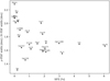 |
Fig. 8 Relation between the star formation efficiency of molecular clouds and the ratio between the widths (in dex) of their volume density PDF and column density PDF. |
4.3 Comparison with other works
4.3.1 Impact of volume density on star formation rates
There is an exhaustive number of works studying the possible column density threshold for star formation in cores (e.g. Elmegreen 2002) or clouds (e.g. Lada et al. 2010; Evans et al. 2014), and the column density distribution is still largely considered as a reliable predictor of star formation (Retter et al. 2021). Similarly, many works relate the column densities to volume densities through a simplistic assumption of geometry, usually a sphere, which then enables considering the threshold in terms of volume density. For example, Lada et al. (2010) derives an extinction threshold of AK = 0.8 mag and from that estimates a volume density threshold of 104 H2 cm−3, very similar to what we obtain in the present work.
Another approach to the study of the relation between the volume density of molecular gas and star formation is based on the observation of so-called dense gas tracers, such as the 3-mm band transitions of HCO+, HNC or HCN. In the wake of the work of Gao & Solomon (2004) on HCN, these molecular lines have been used, due to their high critical densities (ρ ∼ 1 × 10⁴−1 × 10⁵ H2 cm−3), to measure the amount of gas present above these densities and compare it with various tracers of star formation, in molecular clouds or nearby galaxies (e.g. Bigiel et al. 2016; Jiménez-Donaire et al. 2019; Kauffmann et al. 2017). However, it is likely that the close correspondence between the volume density threshold for star formation found in the present study and the densities allegedly traced by HCN(J = 1–0) is a mere coincidence. The critical density is not a hard threshold for the emission of molecular lines, so that not only there is a large spread in the estimation of the volume densities sampled by these tracers (from ∼1 × 10⁴ to almost 1× 10⁶ H2 cm−3), but there is also an increasing amount of arguments questioning whether dense gas tracers do actually trace specifically the dense gas content of molecular clouds (Pety et al. 2017; Shimajiri et al. 2017; Tafalla et al. 2021; Dame & Lada 2023), given that HCN is actually detected over a very broad range of column (and thus volume) densities in molecular clouds – this is among others due to the fact that HCN is mostly observed to be optically thick while its critical density decreases with opacity (e.g. Shirley 2015). In particular Tafalla et al. (2021) argue that HCN(J = 1–0) rather traces the total gas content of clouds, its very linear correlation with column density being a lucky interplay between excitation and chemical abundance effects. In that context, it should be understood that the density threshold for star formation of 2 × 10⁴ H2 cm−3 derived from the Colume volume density reconstructions is a fully independent result, which provides no argument in favour of the use of HCN, HNC or HCO+ lines to trace the star-forming gas in molecular clouds. Conversely, the value of this threshold does not invalidate the use of specific astrochemical tracers such as N2H+ to trace even denser gas in clouds and cores (e.g. Kirk et al. 2016; Pety et al. 2017; Kauffmann et al. 2017).
An interesting approach, which takes a step towards volume density modelling, has been pioneered by Hu et al. (2021). The authors acknowledge that column density measurements are not sufficient to determine accurately the star formation activity, and in particular the free-fall time of molecular clouds. However, rather than trying to directly reconstruct the volume density distribution, they use simulations to build a model which indirectly derives the cloud free-fall time (and therefore the star formation rate) from the column density distribution. A direct comparison with our study based on volume densities is thus unfortunately not possible.
Even more relevant to the present case, Kainulainen et al. (2014) presented a method to derive volume density PDFs of molecular clouds via inverse modelling and applied it to a sample of nearby clouds. Based on their volume density data, Kainulainen et al. (2014) derived a star formation threshold of 5 × 103 cm−3. It is important to recall that Kainulainen et al. (2014) defined star formation threshold as the highest densities in clouds that had no or very little star formation. The threshold we derived in this paper is significantly higher, at 2 × 10⁴ H2 cm−3. However, this difference is likely related not only to differences in definitions of the star formation threshold, but also differences in data sets (spatial resolution, dynamic range, and star formation numbers). In addition to the more limited column densities probed by their extinction data, Kainulainen et al. (2014) mapped their cloud at a coarser resolution of 0.1 pc. For a volume density reconstruction with Colume, a lower resolution has the double effect of reducing the column density peaks by washing them out, and of making the size of the inferred volumes larger – both effects contribute to lowering the reconstructed volume densities, with the former being largely dominant. Figure 9 shows the maximum volume densities and SFE in the clouds that overlap between our and Kainulainen et al. (2014) samples, comparing the cases of the 36.3″ Herschel resolution and of a smoothed, 0.1 pc resolution. The maximum volume densities are heavily affected by resolution, and in particular, many clouds gather around 1–2 × 103 cm−3 in the smoothed resolution. This order-of-magnitude effect is the likely reason for the difference between the star formation thresholds we and Kainulainen et al. (2014) derived. Using the Colume volume density reconstruction along with the Kainulainen et al. (2014) threshold definition would yield a density threshold of 1–1.5 × 10³ H2 cm−3 and 6–10 × 104 H2 cm−3 at 0.1 pc and 36.3″ resolutions respectively, showing that these different approaches yield compatible results.
4.3.2 Volume density inference
The work of Kainulainen et al. (2014) described above is particularly interesting in its attempt to reconstruct volume densities, despite the limitations of the column density data used, and the lack of focus on the spatial distribution (maps) of volume densities.
In that context, another inversion approach for determining volume densities for a generic cloud geometry has been presented by Hasenberger & Alves (2020). Their method, named AVIATOR, is based on the inverse Abel transform of column density data. Hasenberger & Alves (2020) did not systematically apply their method to full molecular clouds, but tested it in the case of two relatively simple globules which are part of our sample, B68 and L1689B, and compared the results with the dedicated modelling results obtained for these globules by Roy et al. (2014). Since the column densities derived in these works differ significantly from the ones derived by the HGBS consortium and used here, a direct comparison of the reconstructed volume densities in not possible. However, the ratios of volume to column density agree remarkably well for B68: the difference for the centre of the globule is of +5% and −4% with respect to Roy et al. (2014) and Hasenberger & Alves (2020) respectively. In the case of L1689B, the match is still reasonably good, at −6% and −23% respectively – this larger difference might be explained by the fact that our reconstruction was influenced by the complex structure of the extended environment of L1689B, while Roy et al. (2014) and Hasenberger & Alves (2020) focused on the dense core only. It is however unclear how AVIATOR would perform in the case of more complex structures such as the ones tackled in the present study; applying it systematically would be an interesting avenue to studying the volume density structure of clouds.
The B68 and L1689B globules are ideal cases for volume density reconstruction, given their simple geometries, isolation which removes any complex contribution from the fore- and background, and lack of significant substructure at higher angular resolutions. Comparisons with volume density estimates in other, more complex environments can show the limitations of the Colume method and of our data set. For example, densities measured at ∼0.1 pc scales in the filamentary structures of nearby, actively star-forming molecular clouds reach values of roughly 105−106 H2 cm−3 (e.g. Hacar et al. 2023, and references therein). The maximum volume densities we infer for clouds like Orion A, CrA, and Taurus L1495 are in this ballpark. In case of less active filamentary clouds like Musca, dedicated works infer slightly lower densities of roughly 5–10 × 104 H2 cm−3 (Kainulainen et al. 2016; Cox et al. 2016); our estimates are in a reasonable agreement with that trend. Overall, it seems that at least in simple filamentary morphologies the estimates are in line with other studies, despite the fact that our model does not take the filamentary aspect into account.
As the geometry becomes more complex, it is expected that our inferred densities become more inaccurate, due to both fragmentation along the line of sight and anisotropy. For example, in the complex star-forming environments of the Aquila Rift and Orion A, dense cores with densities clearly higher than 106 cm−3 have been identified (e.g. Könyves et al. 2015; Shimajiri et al. 2015). Our maximum densities for Aquila and Orion A are about 0.2 and 0.6 × 106 cm−3, respectively. While still within the right order of magnitude, our estimates in this kind of environment become clearly more inaccurate due to the oversimplifying geometrical assumptions of the method.
Another limitation, discussed in the context of Fig. 9, is the question of spatial resolution. Due to the modest angular resolution of Herschel data, we cannot reach spatial scales (and therefore volumes) small enough to be able to probe the densest parts of prestellar cores (e.g. the ∼ 107 H2 cm−3 reached in Orion A (Sahu et al. 2023) derived from ALMA observations with an angular resolution up to 100 times better than Herschel).
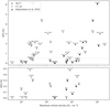 |
Fig. 9 Comparison between the maximum volume densities obtained for the clouds in our sample at the fixed angular resolution of 36.3″ provided by the Herschel telescope, and at the fixed spatial resolution of 0.1 pc used by Kainulainen et al. (2014). The 12 clouds in common between the Kainulainen et al. (2014) sample and ours are highlighted by square markers. The bottom panel is a zoom-in of the area defined by the horizontal dashed lines in the top panel, at the very low SFE relevant for defining a star formation threshold. |
5 Conclusion
In order to study the role of the volume density distribution of molecular clouds in their star formation activity, we developed Colume, an algorithm that performs a simple geometrical inference of the statistical distribution of gas volume density in a cloud based on the morphology of its column density map.
We applied Colume to Herschel-derived maps of column density for 25 nearby molecular clouds, and compared the properties of the obtained volume density distributions with the original column density data, and with the star formation properties of the individual clouds. We observed the following significant trends:
The correlation between the column density and the peak volume density shows a piecewise power law behaviour, with two distinct regimes. At low column densities the exponent of the power law is ∼1; at high column densities this exponent becomes ∼2. The transition between the regimes happens at column densities of the order of 5–10×1022 H2 cm−2, which is compatible with the commonly adopted dense gas limit of AV = 8 mag. The difference between these two correlation regimes is most likely an illustration of the importance of hierarchical fragmentation in dense gas;
We tested two different dense gas descriptors (dense gas fraction and density contrast), and applied them to the column density and volume density distributions of the clouds. Out these four different measurements, the volume-density-based dense gas fraction has the tightest correlation with the star formation efficiency of the clouds. This illustrates that star formation laws are controlled by physical quantities (such as volume density), not by observed quantities (such as column density), and underlines the importance of retrieving these physical quantities from observational data, even if indirectly;
The correlation between the star formation efficiency and the volume-density-based dense gas fraction (or between the star formation rate and the mass of dense gas) is tightest with a low-density threshold (which separates the bulk of the cloud from the diffuse background) set at 2 × 10² H2 cm−3 and a high-density threshold (which separates the dense star-forming gas from the bulk of the cloud) set at 2 × 10⁴ H2 cm−3.
Many refinements in the treatment of the cloud morphology or in the aggregation of additional observational data could be implemented in order to improve the volume density reconstruction, but we have already shown with our results obtained with a purposefully simplistic approach that reconstructing volume density has the potential of being an extremely powerful tool for studying the ISM. Follow-up studies involving volume density statistics, star formation properties, and the chemistry of clouds using Colume will further reveal this potential.
Data availability
Supplementary figures, in particular the equivalents of Fig. 4 for all clouds in the studied sample, are available at the following address: https://zenodo.org/records/14360623
The Colume code is referenced here: https://www.ascl.net/2503.034, and available for downloading with its dependencies here: https://github.com/jan-orkisz/colume
Acknowledgements
This research has made use of data from the Herschel Gould Belt survey (HGBS) project (http://gouldbelt-herschel.cea.fr). The HGBS is a Herschel Key Programme jointly carried out by SPIRE Specialist Astronomy Group 3 (SAG 3), scientists of several institutes in the PACS Consortium (CEA Saclay, INAF-IFSI Rome and INAF-Arcetri, KU Leuven, MPIA Heidelberg), and scientists of the Herschel Science Center (HSC). Jan Orkisz acknowledges funding from the Swedish Research Council, grant No. 201703864. The authors thank Maryvonne Gerin for helpful comments on the writing of this paper.
Appendix A Tests on simulated data
A.1 Data and test procedure
Given that our volume density estimation algorithm is intrinsically assuming that the density distribution of clouds is hierarchically fragmented into centrally concentrated sub-regions, we have to choose astrophysical simulations which match this description reasonably well in order to obtain meaningful results. For that purpose, we selected the simulation data presented and studied by Ibáñez-Mejía et al. (2017) and Chira et al. (2019), available as part of the CATS (Burkhart et al. 2020) database. This simulation is a zoom-in focused on star-forming clouds in a galactic context. A portion of galactic disc was simulated including ideal compressible magneto-hydrodynamics (MHD), gas heating and cooling, supernova driving and a static gravitational potential. Three dense clouds were selected in this environment and their collapse under the effect of selfgravity was followed at a higher resolution, with snapshots being taken every 0.1 Myr. The simulation was run using the FLASH (Fryxell et al. 2000; Dubey et al. 2008) adaptive mesh refinement code.
The data used for our tests is the snapshot of a cloud with an initial mass M = 4 × 10³ M⊙, after 3 Myr of evolution under the effect of self-gravity. From this snapshot we extracted a 40 × 40 × 40 pc cube of volume density values (expressed in H cm−3) with a adaptive resolution ranging from 0.4 to 0.1 pc. The volume density distribution (Fig. A.1) of the cloud is tri-modal, with most of the volume of the simulation cube corresponding to densities around 1 × 10⁻³ and 1 × 10⁻¹ H cm−3. Most of the mass of the cloud is however found in the last peak of the PDF, at densities higher than 1 H cm−3. The densities are nevertheless not particularly high, not even reaching 1 × 10⁵ H cm−3. This is compatible with the volume densities estimated for low-density filamentary networks (e.g. Orkisz et al. 2019) or low-mass cores (e.g. Kirk et al. 2016), but filaments or dense cores can also reach densities an order of magnitude larger than this (e.g. Teixeira et al. 2016). The density distribution of this simulated cloud is therefore not perfectly representative of the most massive star-forming clouds in our sample.
In order to generate simulated data sets, the simulated cube is simply summed along each of its axes to produce three column density maps. At this stage, in order to simulate the presence of a diffuse fore- and background, a uniform offset of 0.1 H cm−3 is added to the cube – this has the consequence of virtually removing the low-density peaks in the volume density PDF, and adds an offset of 1.23 × 10¹⁹ H cm−2 to the column density maps. The median column density value is 2.2 × 10¹⁹ H cm−2 and the maximum 3.6–5.9 ×10²² H cm−2 depending on the projection.
The nine (three clean, six noisy) maps were then passed to the Colume code with an arbitrary distance and the matching angular resolution, with 800 sampling levels with the standard inverse log percentile binning (Sect. B). The maps of mean and peak density along the line of sight were generated, as well as volume density PDFs, and compared with the reference values of the noiseless simulated cube.
A.2 Results
A.2.1 Reliability of the density estimation in the ideal case
The noiseless column density maps produced from a simulated cloud isolated within a cube are the ideal scenario in which to run a volume density reconstruction. Real observational data are noisy, the fore- and background contamination as well as the limited observational field make it difficult if not impossible to define clearly the boundaries of the cloud, not to mention our ignorance in most cases regarding the isotropy of the cloud. However, this ideal case is still a necessary test-bed for the Colume code.
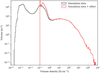 |
Fig. A.1 Volume density distribution in the simulated test cloud, which has an initial mass M = 4 × 10³ M⊙ and lies in a 40 × 40 × 40 pc cube. An offset density is added to the cube to simulate a diffuse foreground and background when simulating column density observations. |
By construction, the Colume method is conservative in terms of total mass, down to sampling precision – this is confirmed in this test with a precision of ≲10−5. In the particular case of this test, this is also true on a pixel-by-pixel basis: since the shape of the original object is really a cube, the geometry of the outer envelope of the cloud is perfectly reconstructed.
Figure A.2 shows the quality of reconstruction of the peak volume density reached along each line of sight for the x-axis projection of the cloud (the y and z projections show similar behaviours). We can see that the reconstructed peak density is typically underestimated by up to an order of magnitude; however, this bias is not uniform throughout the density range. As it can be seen from the upper right and lower left panels of Fig. A.2, the reconstructed peak density is very close to the original for very low (≲1 H cm−3) and high (≳ 104 H cm−3) volume densities. At intermediate densities, the peak volume densities are much more underestimated. This can be understood in terms of scale and structure of the gas (which is well illustrated by the lower left panel of Fig. A.2). The lowest and highest volume densities correspond to the envelope of the cloud and to dense cores respectively, which have rather isotropic shapes. On the other hand, at intermediate densities, the gas is mostly distributed into sheets and filaments, for which the isotropy assumption which underlies our volume reconstruction in inappropriate – the estimated volumes are too large, and consequently the densities too low. This scale-dependent effect is present for all the density increments encountered along a given line of sight, and the peak volume density, being the sum of all these increments, displays this bias in a particularly visible way.
The volume density PDF is also a crucial element in order to derive quantity such as the dense gas fraction or density contrast. Figure A.3 shows that the reconstruction of this PDF is very consistent no matter what the projection angle is.
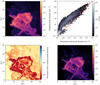 |
Fig. A.2 Estimation of the peak volume density along the line of sight from a noiseless column density map. Top left: Original noiseless data. Top right: Joint histogram of the original vs. reconstructed peak volume densities. Bottom left: Map of the ratio of reconstructed-to-original peak volume densities. Bottom right: Reconstructed map of peak volume densities along the line of sight. |
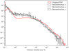 |
Fig. A.3 . True volume density distribution of the simulated data cube (Fig. A.1), compared to the reconstructed distributions based on the analysis of the projected column density maps. |
A.2.2 Influence of noise
In order to test the behaviour of the Colume code when dealing with imperfect data, we added two different patterns of Gaussian noise to the clean column density maps. The first is a noise with a uniform noise amplitude of 3.7 × 10¹⁹ H cm−2, corresponding to three times the background level – the signal-to-noise ratio-therefore varies between 1/3 and ∼1000 throughout the maps. The second pattern is a constant signal-to-noise of 10 (Gaussian amplitude proportional to the signal).
Figures A.4 and A.5 show the comparison between the reconstructed volume densities and the original (noiseless) data.
The uniform noise (Fig. A.4) heavily affects the regions of low density, but this has consequences also on high-density regions despite their very high signal-to-noise ratio. What happens is that regions which otherwise would be smooth are disrupted by noise on a pixel-by-pixel basis, each noisy pixel being effectively treated as a small dense core. This results in many low-density pixels being incorrectly reconstructed as (very) high mean and peak densities, which is obvious in the joint histograms of Fig. A.4 (panels 2 and 6). The case with constant signal-to-noise (Fig. A.5) shows a very limited impact of noise on the reconstructed mean densities, and a weaker impact on peak densities than in the case of uniform noise.
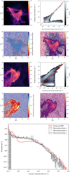 |
Fig. A.4 Effect of added noise on volume density reconstruction. Top four panels: Same as Fig. A.2, but for the mean volume density along the line of sight, for a different projection, and with added uniform noise. Middle four panels: Same as above, but for the peak volume density along the line of sight, and for a different projection. Bottom: Same as Fig. A.3, but with added uniform noise. |
Appendix B Column density sampling
As described in Sect. 2.1.2, the size of the generated volume density data set is of the order of X × Y × S, where X × Y are dimensions of the column density map and S is the number of column density increments. The native number of increments, S0, is equal to the number of unique values in the column density map, with S0 ≤ X × Y – in practice with high-precision data and in the presence of noise S0 ∼ X × Y. The native maximum size of the volume density data set is thus of the order of ≲ (X × Y)2. Such a size is unmanageable in terms of random-access memory requirements during the computation: once accounted for the different data by-products, buffers, and for the digital precision used for the data, even a moderate field such as the 400 × 400 pixel test field used in Appendix A requires several terabytes of RAM. A sampling such that S ≪ S0 is therefore necessary, with the constraint of recovering as much as possible of the detailed cloud structure.
Two main approaches are taken to sample the column density values: one called the min-max approach, which is agnostic to the distribution of column density values except for its minimum and maximum, and a percentile approach, which as the name suggests follows the percentiles of the distribution; we note that we consider the distribution of unique column density values rather than the column density PDF of the entire field. In both cases, the spacing of the sampling bins can be set in different ways, the ones we implemented are the following: a linear spacing (where the difference between successive bins is constant), a conventional logarithmic (log) spacing (where the ratio between successive bins is constant), and an inverse logarithmic (i-log) spacing, which is the base-10 logarithm of a linear spacing, rescaled to the range of the data. For a number of samples S, with extrema Nmin and Nmax, and percentiles of distribution Y being denoted px(Y) (with x between 0 and 100), the i-th bin threshold Ni is thus defined as follows:
Min-Max linear

Min-Max log

Min-Max i-log

Percentiles linear

Percentiles log

Percentiles i-log

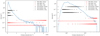 |
Fig. B.1 Comparison of the bin locations for the various sampling options implemented in Colume applied to the column density distribution of the Cha II cloud, with a coarse 50-level sampling, in linear and logarithmic scales. |
The definitions of the i-log scales and of the percentiles log scale are somewhat arbitrary, due to the impossibility to define in a unique, natural way a logarithmic function which maps the [0, 1] range on itself. The i-log definition is thus chosen to be the most natural for percentiles, and the percentiles log scale is defined so that its first bin above 0 has the same value as in the percentiles linear sampling.
The bins created by six different sampling methods are illustrated in Fig. B.1 for the case of the Cha II cloud column density distribution, with a very coarse 50-level sampling. The choice of sampling is dependent on what one wants to achieve, and in particular on which column density range one wants to prioritise. The log and i-log spacings sample in more detail the low and high column densities, respectively. The min-max approach offers the advantage of simplicity of implementation and interpretation, but the bins can be used in a sub-optimal way, for example sampling too densely a part of the column density distribution which is not very populated, to the point of creating many empty bins. Conversely, the percentile approach yields a bin spacing that is not intuitive, but adapts directly to the structure of the data. The typical shape of column density PDFs, with a main log-normal-like peak and a long power-law-like tail (see Spilker et al. (2021) for a discussion of PDF shapes) also entails that the min-max approach samples in far more detail the tail than the peak of the distribution, while the opposite is true for the percentiles approach. The combination of these effects yields sampling options which put more or less emphasis on the description of the low, intermediate or high column densities. Figures B.2 and B.3 illustrate the results of the sampling choice on the global volume density PDF and the peak volume density map of the Cha II cloud with a 50-level sampling, compared to the reference 2000-level i-log percentile sampling used in this study.
One can see that, in agreement with the effects visible in Fig. B.1, the linear and i-log min-max samplings fail to reproduce the low volume density envelope of the cloud, while the linear and log percentile samplings are unable to give detailed view of the densest regions. The log min-max and i-log percentile samplings on the other hand are able to recover reliably a broader range of volume densities.
While it is of high importance when studying star formation to have a detailed view of the high-density regions of molecular clouds, this cannot be completely at the expense of other density ranges. This is due to the increment-based nature of the volume density reconstruction: the high volume densities are not reconstructed independently, but as increments built on top of a lower density structure. While a small error in the reconstruction of the lower volume densities has negligible effects on the values of the highest volume densities in a cloud (as discussed in Sect. 4.1), a significant bias in the sampling of low to intermediate column densities can result in a bias in the reconstructed high volume density values – this is for example visible for the i-log min-max sampling in Figs. B.2 and B.3, where the high volume densities, while very finely sampled, are biased by a factor of a few with respect to the reference. On the other hand, given that the volume-density reconstruction is mass-conservative, even if the sampling of the highest densities is not extremely fine, the loss of detail would affect the morphology but not the mass of the high-density regions, and dense gas measurements (Sect. 3.2.1) would be largely unaffected.
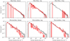 |
Fig. B.2 Effects of sampling options on the global volume density PDF, illustrated by comparing coarse, 50-level volume density reconstructions with a 2000-level benchmark, for the Cha II cloud. |
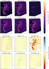 |
Fig. B.3 Effects of sampling options on the peak volume density maps, for the Cha II cloud. Top: Peak volume density maps obtained with different coarse, 50-level volume density reconstructions. Bottom: Ratio of these maps to the reference peak volume density map (obtained with a 2000-level i-log percentile sampling). |
In that perspective, the min-max logarithmic sampling and the i-log percentile sampling perform therefore comparably well for our purpose. In the end, our choice of the i-log percentile sampling was motivated by the wish to optimise the sampling performance without having to worry about the diversity of field sizes and column density PDF shapes, and in particular to avoid empty bins.
Appendix C Effect of anisotropy
One of the key over-simplifications of the cloud structure model used in Colume is the assumption of isotropy at all scales (α = 1). Not only is this assumption in general not true, but the degree of isotropy or anisotropy strongly depends on the studied scale (or contour area): on projected areas above 1 pc2, clouds might or might not be isotropic, for areas smaller than 0.1 × 0.1 pc2, dense cores are generally considered to be quite isotropic (see e.g. B68), and, in between, all sorts of clumps, sheets and filaments can have various degrees of isotropy, in particular high-aspect-ratio filaments of projected areas of ∼ 1 × 0.1 pc2.
It is therefore not sufficient to fix a value of α ≠ 1 to recover the effects of anisotropic gas distribution in a molecular cloud: α need to vary with scale. The simplest approach is to have a fixed prescription for α as a function of  . We tested the effects of this approach in comparison with the isotropic computation for a well-known and highly anisotropic cloud, namely Orion A. It is also one of the most complex and massive clouds in our sample, which makes the volume density inference particularly challenging.
Orion A is famous for its cometary shape, with a high aspect ratio in the plane of the sky that actually translates to a filamentary shape in three dimension (Bally 2008; Großschedl et al. 2018; Rezaei Kh. et al. 2020). The molecular gas in Orion A displays an elongated shape of about 40 × 5 pc in the plane of the sky – and we here omit the fact that while the head of the cloud (northern part, harbouring to the Integral-Shaped Filament) lies in the plane of the sky, its tail is highly inclined, leading to an actual length of the cloud of about 70 pc (Großschedl et al. 2018). While taking into account the variable inclination of the main structures would exemplify even further the case of a high-aspect-ratio cloud, it would also increase the complexity of the anisotropic model, so we limited ourselves to the simpler assumption of a cloud lying parallel to the plane of the sky. We thus assumed that on the largest scales (40 × 5 = 200 pc2), the cloud is roughly cylindrical, with its depth equal to its width, despite a projected aspect ratio of ∼8 (thus  ). And on small scales (0.1 × 0.1 = 0.01 pc2), we assumed that cores are isotropic (α = 1). These two constraints were smoothly joined in log-space by the following cosine interpolation, illustrated in Fig. C.1:
 (C.1)
(C.1)
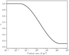 |
Fig. C.1 Variation of anisotropy factor α as a function of scale in the case of Orion A. |
An overview of the compared outputs of the isotropic and anisotropic models for volume density can be found in Fig. C.2; we also discuss in more details the comparison of the peak volume densities and the global volume density distributions obtained by the two different models.
Since on the largest scales the reconstructed volume is smaller than in the isotropic case, the lowest reconstructed densities increments are automatically higher – which is visible in the left panel of Fig. C.3 as a shift towards higher densities of the entire lower end of the PDF. On the other hand the smallest volumes, which mostly correspond to high-density regions, are essentially treated in the same way by the isotropic and anisotropic models. Reconstructing volume density from increments means that a density increase on the first increments is reflected for all higher densities, but given the shape of the volume density distribution, this has a negligible effect on the highest volume densities (as we are adding a few tens of H2 cm−3 to densities of more than 104 H2 cm−3). This is visible on the left panel of Fig. C.3 where at high volume densities the PDF of the anisotropic model lies above the one of the isotropic model, but barely so. We can also see in the right panel of the same figure that the anisotropic model reconstructs less (technically, zero) of the lowest volume densities of the isotropic model; it reconstructs significantly more medium densities (∼2 × 10²− 2 × 10³ H2 cm−3) as a combined effect of accumulated excesses in low-volume density increments and of α still significantly lower than 1; and while it also reconstructs more high volume densities, this excess decreases in a power-law-like manner.
The same effect is illustrated in a different way by the comparison of peak volume densities in Fig. C.5. The maps produced by the isotropic and anisotropic models (panels 2 and 3) are remarkably similar, except for the fact that the lower end of the scale of the anisotropic map is shifted to higher densities. The difference between these two maps (panel 4) shows a trend by which at higher densities (column or peak volume), the difference is larger – which is the effects of the accumulation of small increases in volume density increments. This difference can be as much as 104 H2 cm−3. On the other hand we can clearly see that the ratio of these two peak volume densities (panel 5) reaches almost 1 in the highest density regions: a difference of 104 H2 cm−3 represent only a few per cent, if relative to values of nearly 106 H2 cm−3.
The same trends (difference increasing with density, ratio decreasing from  to 1) are illustrated in the form of joint histograms in Fig. C.4. In summary, while in absolute terms variations in the anisotropy parameter α have an impact at all scales smaller than the scale at which anisotropy is present, in relative terms volume density is significantly affected only by anisotropy at scales close to those corresponding to the considered range of density.
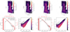 |
Fig. C.2 Left: Same four panels as Fig. 4, for the Orion A giant molecular cloud. Right: Same, but with anisotropy taken into account. |
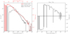 |
Fig. C.3 Left: Comparison of the column density PDF with the global isotropic and anisotropic volume density PDFs derived for Orion A. Right: PDF of the difference between the global volume density distribution derived by the anisotropic and isotropic model (presented on a symmetric logarithmic scale). |
The final comparison that we need to do in the scope of this paper is the question of the fraction of dense gas. Taking the same volume density threshold, we obtain an increase of 14.9% in  for Orion A when using this anisotropic model which is not as little as the peak volume densities would suggest, but is difficult to comment on given that Orion A is not an outlier in the density versus SFE relation. For comparison, we also computed an anisotropic model where Orion A is assumed to be a sheet: this time, the depth along the line of sight is assumed to be equivalent to the largest, instead of the smallest, dimension in the plane of the sky, so
  for the largest scales. We find this time a decrease of 13.7% for
  . Lack of knowledge about the bulk line-of-sight dimension of a cloud can thus lead to a 33% difference in inferred dense gas fraction and thus star formation efficiency. It is not sufficient, however, to explain order-of-magnitude differences in SFE between apparently similar clouds, such as reported for Orion A and the California Cloud (Rezaei Kh. & Kainulainen 2022), or Orion A and B (Orkisz et al. 2019): in both cases, the distribution and isotropy of structures at intermediate scales (fragmentation and dimension of sub-clouds, fraction of mass accumulated into dense filaments) matters greatly in order to estimate properly the statistical distribution of dense gas in a cloud and its contribution to star formation. Incorporating priors and measurements on fragmentation and anisotropy for each contour at each scale is however beyond the current capabilities of the Colume code.
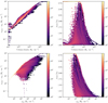 |
Fig. C.4 Joint distribution of the column density (top) or isotropic peak volume density (bottom) with the difference between the isotropic and anisotropic peak volume densities (left) or their ratio (right). |
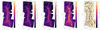 |
Fig. C.5 Comparison of the effect of scale-dependent anisotropy on density maps. From left to right: Column density map used as a prior; peak volume density map obtained with the isotropic model; peak volume density map obtained with the anisotropic model; difference between the two peak volume density maps; ratio between the two peak volume density maps. |
References
- Alves, J. F., Lada, C. J., & Lada, E. A. 2001, Nature, 409, 159 [NASA ADS] [CrossRef] [Google Scholar]
- Alves, J., Lombardi, M., & Lada, C. J. 2017, A&A, 606, L2 [NASA ADS] [CrossRef] [EDP Sciences] [Google Scholar]
- Alves de Oliveira, C., Schneider, N., Merín, B., et al. 2014, A&A, 568, A98 [NASA ADS] [CrossRef] [EDP Sciences] [Google Scholar]
- André, P., Men’shchikov, A., Bontemps, S., et al. 2010, A&A, 518, L102 [NASA ADS] [CrossRef] [EDP Sciences] [Google Scholar]
- Arzoumanian, D., André, P., Didelon, P., et al. 2011, A&A, 529, L6 [NASA ADS] [CrossRef] [EDP Sciences] [Google Scholar]
- Arzoumanian, D., André, P., Könyves, V., et al. 2019, A&A, 621, A42 [NASA ADS] [CrossRef] [EDP Sciences] [Google Scholar]
- Astropy Collaboration (Robitaille, T. P., et al.) 2013, A&A, 558, A33 [NASA ADS] [CrossRef] [EDP Sciences] [Google Scholar]
- Astropy Collaboration (Price-Whelan, A. M., et al.) 2018, AJ, 156, 123 [Google Scholar]
- Bacchini, C., Fraternali, F., Iorio, G., & Pezzulli, G. 2019a, A&A, 622, A64 [NASA ADS] [CrossRef] [EDP Sciences] [Google Scholar]
- Bacchini, C., Fraternali, F., Pezzulli, G., et al. 2019b, A&A, 632, A127 [NASA ADS] [CrossRef] [EDP Sciences] [Google Scholar]
- Bally, J. 2008, in Handbook of Star Forming Regions, Volume I, 4, ed. B. Reipurth, 459 [Google Scholar]
- Benedettini, M., Pezzuto, S., Schisano, E., et al. 2018, A&A, 619, A52 [NASA ADS] [CrossRef] [EDP Sciences] [Google Scholar]
- Bigiel, F., Leroy, A. K., Jiménez-Donaire, M. J., et al. 2016, ApJ, 822, L26 [NASA ADS] [CrossRef] [Google Scholar]
- Bontemps, S., André, P., Könyves, V., et al. 2010, A&A, 518, L85 [NASA ADS] [CrossRef] [EDP Sciences] [Google Scholar]
- Bresnahan, D., Ward-Thompson, D., Kirk, J. M., et al. 2018, A&A, 615, A125 [NASA ADS] [CrossRef] [EDP Sciences] [Google Scholar]
- Bron, E., Daudon, C., Pety, J., et al. 2018, A&A, 610, A12 [CrossRef] [EDP Sciences] [PubMed] [Google Scholar]
- Brunt, C. M., Federrath, C., & Price, D. J. 2010a, MNRAS, 405, L56 [CrossRef] [Google Scholar]
- Brunt, C. M., Federrath, C., & Price, D. J. 2010b, MNRAS, 403, 1507 [Google Scholar]
- Burkhart, B., & Mocz, P. 2019, ApJ, 879, 129 [NASA ADS] [CrossRef] [Google Scholar]
- Burkhart, B., Appel, S. M., Bialy, S., et al. 2020, ApJ, 905, 14 [Google Scholar]
- Chabrier, G. 2003, PASP, 115, 763 [Google Scholar]
- Chira, R. A., Ibáñez-Mejía, J. C., Mac Low, M. M., & Henning, T. 2019, A&A, 630, A97 [NASA ADS] [CrossRef] [EDP Sciences] [Google Scholar]
- Clarke, S. D., Whitworth, A. P., Spowage, R. L., et al. 2018, MNRAS, 479, 1722 [Google Scholar]
- Cox, N. L. J., Arzoumanian, D., André, P., et al. 2016, A&A, 590, A110 [NASA ADS] [CrossRef] [EDP Sciences] [Google Scholar]
- Dame, T. M., & Lada, C. J. 2023, ApJ, 944, 197 [NASA ADS] [CrossRef] [Google Scholar]
- de Geus, E. J., de Zeeuw, P. T., & Lub, J. 1989, A&A, 216, 44 [NASA ADS] [Google Scholar]
- Di Francesco, J., Keown, J., Fallscheer, C., et al. 2020, ApJ, 904, 172 [NASA ADS] [CrossRef] [Google Scholar]
- Dubey, A., Fisher, R., Graziani, C., et al. 2008, in Astronomical Society of the Pacific Conference Series, 385, Numerical Modeling of Space Plasma Flows, eds. N. V. Pogorelov, E. Audit, & G. P. Zank, 145 [NASA ADS] [Google Scholar]
- Dunham, M. M., Allen, L. E., Evans, Neal J., I., et al. 2015, ApJS, 220, 11 [Google Scholar]
- Elmegreen, B. G. 2002, ApJ, 577, 206 [CrossRef] [Google Scholar]
- Evans, Neal J., I., Allen, L. E., Blake, G. A., et al. 2003, PASP, 115, 965 [Google Scholar]
- Evans, Neal J., I., Dunham, M. M., Jørgensen, J. K., et al. 2009, ApJS, 181, 321 [NASA ADS] [CrossRef] [Google Scholar]
- Evans, Neal J., I., Heiderman, A., & Vutisalchavakul, N. 2014, ApJ, 782, 114 [CrossRef] [Google Scholar]
- Fazio, G. G., Hora, J. L., Allen, L. E., et al. 2004, ApJS, 154, 10 [Google Scholar]
- Federrath, C., & Klessen, R. S. 2013, ApJ, 763, 51 [Google Scholar]
- Fiorellino, E., Elia, D., André, P., et al. 2021, MNRAS, 500, 4257 [Google Scholar]
- Forbrich, J., Lada, C. J., Muench, A. A., Alves, J., & Lombardi, M. 2009, ApJ, 704, 292 [NASA ADS] [CrossRef] [Google Scholar]
- Fryxell, B., Olson, K., Ricker, P., et al. 2000, ApJS, 131, 273 [Google Scholar]
- Gao, Y., & Solomon, P. M. 2004, ApJ, 606, 271 [NASA ADS] [CrossRef] [Google Scholar]
- Goldsmith, P. F., Heyer, M., Narayanan, G., et al. 2008, ApJ, 680, 428 [Google Scholar]
- Green, G. M., Schlafly, E., Zucker, C., Speagle, J. S., & Finkbeiner, D. 2019, ApJ, 887, 93 [NASA ADS] [CrossRef] [Google Scholar]
- Großschedl, J. E., Alves, J., Meingast, S., et al. 2018, A&A, 619, A106 [Google Scholar]
- Gutermuth, R. A., Megeath, S. T., Myers, P. C., et al. 2009, ApJS, 184, 18 [Google Scholar]
- Güver, T., & Özel, F. 2009, MNRAS, 400, 2050 [Google Scholar]
- Hacar, A., Clark, S. E., Heitsch, F., et al. 2023, in Astronomical Society of the Pacific Conference Series, 534, Protostars and Planets VII, eds. S. Inutsuka, Y. Aikawa, T. Muto, K. Tomida, & M. Tamura, 153 [NASA ADS] [Google Scholar]
- Harris, C. R., Millman, K. J., van der Walt, S. J., et al. 2020, Nature, 585, 357 [NASA ADS] [CrossRef] [Google Scholar]
- Hasenberger, B., & Alves, J. 2020, A&A, 633, A132 [NASA ADS] [CrossRef] [EDP Sciences] [Google Scholar]
- Heyer, M., & Dame, T. M. 2015, ARA&A, 53, 583 [Google Scholar]
- Hildebrand, R. H. 1983, QJRAS, 24, 267 [NASA ADS] [Google Scholar]
- Hu, Z., Krumholz, M. R., Federrath, C., Pokhrel, R., & Gutermuth, R. A. 2021, MNRAS, 502, 5997 [Google Scholar]
- Ibáñez-Mejía, J. C., Mac Low, M.-M., Klessen, R. S., & Baczynski, C. 2017, ApJ, 850, 62 [Google Scholar]
- Jiménez-Donaire, M. J., Bigiel, F., Leroy, A. K., et al. 2019, ApJ, 880, 127 [CrossRef] [Google Scholar]
- Kainulainen, J., Federrath, C., & Henning, T. 2013, A&A, 553, L8 [NASA ADS] [CrossRef] [EDP Sciences] [Google Scholar]
- Kainulainen, J., Federrath, C., & Henning, T. 2014, Science, 344, 183 [NASA ADS] [CrossRef] [Google Scholar]
- Kainulainen, J., Hacar, A., Alves, J., et al. 2016, A&A, 586, A27 [NASA ADS] [CrossRef] [EDP Sciences] [Google Scholar]
- Kainulainen, J., Rezaei, K. S., Spilker, A., & Orkisz, J. 2022, A&A, 659, L6 [NASA ADS] [CrossRef] [EDP Sciences] [Google Scholar]
- Kauffmann, J., Goldsmith, P. F., Melnick, G., et al. 2017, A&A, 605, L5 [NASA ADS] [CrossRef] [EDP Sciences] [Google Scholar]
- Kirk, J. M., Ward-Thompson, D., Palmeirim, P., et al. 2013, MNRAS, 432, 1424 [Google Scholar]
- Kirk, H., Di Francesco, J., Johnstone, D., et al. 2016, ApJ, 817, 167 [NASA ADS] [CrossRef] [Google Scholar]
- Klessen, R. S. 2000, ApJ, 535, 869 [NASA ADS] [CrossRef] [Google Scholar]
- Könyves, V., André, P., Men’shchikov, A., et al. 2015, A&A, 584, A91 [Google Scholar]
- Könyves, V., André, P., Arzoumanian, D., et al. 2020, A&A, 635, A34 [Google Scholar]
- Kóspál, Á., Prusti, T., Cox, N. L. J., et al. 2012, A&A, 541, A71 [NASA ADS] [CrossRef] [EDP Sciences] [Google Scholar]
- Kruijssen, J. M. D., Longmore, S. N., Elmegreen, B. G., et al. 2014, MNRAS, 440, 3370 [Google Scholar]
- Krčo, M., & Goldsmith, P. F. 2016, ApJ, 822, 10 [Google Scholar]
- Lada, C. J., Lombardi, M., & Alves, J. F. 2010, ApJ, 724, 687 [Google Scholar]
- Lada, C. J., Forbrich, J., Lombardi, M., & Alves, J. F. 2012, ApJ, 745, 190 [NASA ADS] [CrossRef] [Google Scholar]
- Ladjelate, B., André, P., Könyves, V., et al. 2020, A&A, 638, A74 [NASA ADS] [CrossRef] [EDP Sciences] [Google Scholar]
- Lallement, R., Vergely, J. L., Babusiaux, C., & Cox, N. L. J. 2022, A&A, 661, A147 [NASA ADS] [CrossRef] [EDP Sciences] [Google Scholar]
- Leike, R. H., Glatzle, M., & Enßlin, T. A. 2020, A&A, 639, A138 [NASA ADS] [CrossRef] [EDP Sciences] [Google Scholar]
- Lewis, J. A., Lada, C. J., Bieging, J., et al. 2021, ApJ, 908, 76 [CrossRef] [Google Scholar]
- Lombardi, M., Bouy, H., Alves, J., & Lada, C. J. 2014, A&A, 566, A45 [NASA ADS] [CrossRef] [EDP Sciences] [Google Scholar]
- Marsh, K. A., Kirk, J. M., André, P., et al. 2016, MNRAS, 459, 342 [Google Scholar]
- Megeath, S. T., Gutermuth, R., Muzerolle, J., et al. 2012, AJ, 144, 192 [NASA ADS] [CrossRef] [Google Scholar]
- Megeath, S. T., Gutermuth, R., Muzerolle, J., et al. 2016, AJ, 151, 5 [Google Scholar]
- Men’shchikov, A., André, P., Didelon, P., et al. 2010, A&A, 518, L103 [Google Scholar]
- Miville-Deschênes, M. A., Martin, P. G., Abergel, A., et al. 2010, A&A, 518, L104 [NASA ADS] [CrossRef] [EDP Sciences] [Google Scholar]
- Orkisz, J. H., Peretto, N., Pety, J., et al. 2019, A&A, 624, A113 [NASA ADS] [CrossRef] [EDP Sciences] [Google Scholar]
- Padoan, P., Federrath, C., Chabrier, G., et al. 2014, in Protostars and Planets VI, eds. H. Beuther, R. S. Klessen, C. P. Dullemond, & T. Henning, 77 [Google Scholar]
- Palmeirim, P., André, P., Kirk, J., et al. 2013, A&A, 550, A38 [NASA ADS] [CrossRef] [EDP Sciences] [Google Scholar]
- Peretto, N., André, P., Könyves, V., et al. 2012, A&A, 541, A63 [NASA ADS] [CrossRef] [EDP Sciences] [Google Scholar]
- Pety, J., Guzmán, V. V., Orkisz, J. H., et al. 2017, A&A, 599, A98 [NASA ADS] [CrossRef] [EDP Sciences] [Google Scholar]
- Pezzuto, S., Elia, D., Schisano, E., et al. 2012, A&A, 547, A54 [NASA ADS] [CrossRef] [EDP Sciences] [Google Scholar]
- Pezzuto, S., Benedettini, M., Di Francesco, J., et al. 2021, A&A, 645, A55 [EDP Sciences] [Google Scholar]
- Pineda, J. L., Goldsmith, P. F., Chapman, N., et al. 2010, ApJ, 721, 686 [NASA ADS] [CrossRef] [Google Scholar]
- Polychroni, D., Schisano, E., Elia, D., et al. 2013, ApJ, 777, L33 [CrossRef] [Google Scholar]
- Rebull, L. M., Padgett, D. L., McCabe, C. E., et al. 2010, ApJS, 186, 259 [NASA ADS] [CrossRef] [Google Scholar]
- Retter, B., Hatchell, J., & Naylor, T. 2021, MNRAS, 507, 1904 [Google Scholar]
- Rezaei Kh., S., & Kainulainen, J. 2022, ApJ, 930, L22 [NASA ADS] [CrossRef] [Google Scholar]
- Rezaei Kh., S., Bailer-Jones, C. A. L., Soler, J. D., & Zari, E. 2020, A&A, 643, A151 [EDP Sciences] [Google Scholar]
- Rieke, G. H., Young, E. T., Engelbracht, C. W., et al. 2004, ApJS, 154, 25 [Google Scholar]
- Roy, A., Martin, P. G., Polychroni, D., et al. 2013, ApJ, 763, 55 [Google Scholar]
- Roy, A., André, P., Palmeirim, P., et al. 2014, A&A, 562, A138 [NASA ADS] [CrossRef] [EDP Sciences] [Google Scholar]
- Rygl, K. L. J., Benedettini, M., Schisano, E., et al. 2013, A&A, 549, L1 [NASA ADS] [CrossRef] [EDP Sciences] [Google Scholar]
- Sadavoy, S. I., di Francesco, J., André, P., et al. 2012, A&A, 540, A10 [NASA ADS] [CrossRef] [EDP Sciences] [Google Scholar]
- Sadavoy, S. I., Di Francesco, J., André, P., et al. 2014, ApJ, 787, L18 [NASA ADS] [CrossRef] [Google Scholar]
- Sahu, D., Liu, S.-Y., Johnstone, D., et al. 2023, ApJ, 945, 156 [Google Scholar]
- Schneider, N., André, P., Könyves, V., et al. 2013, ApJ, 766, L17 [NASA ADS] [CrossRef] [Google Scholar]
- Shimajiri, Y., Kitamura, Y., Nakamura, F., et al. 2015, ApJS, 217, 7 [NASA ADS] [CrossRef] [Google Scholar]
- Shimajiri, Y., André, P., Braine, J., et al. 2017, A&A, 604, A74 [NASA ADS] [CrossRef] [EDP Sciences] [Google Scholar]
- Shirley, Y. L. 2015, PASP, 127, 299 [Google Scholar]
- Sicilia-Aguilar, A., Roccatagliata, V., Getman, K., et al. 2014, A&A, 562, A131 [NASA ADS] [CrossRef] [EDP Sciences] [Google Scholar]
- Skrutskie, M. F., Cutri, R. M., Stiening, R., et al. 2006, AJ, 131, 1163 [NASA ADS] [CrossRef] [Google Scholar]
- Spilker, A., Kainulainen, J., & Orkisz, J. 2021, A&A, 653, A63 [NASA ADS] [CrossRef] [EDP Sciences] [Google Scholar]
- Suri, S., Sánchez-Monge, A., Schilke, P., et al. 2019, A&A, 623, A142 [NASA ADS] [CrossRef] [EDP Sciences] [Google Scholar]
- Tafalla, M., Usero, A., & Hacar, A. 2021, A&A, 646, A97 [NASA ADS] [CrossRef] [EDP Sciences] [Google Scholar]
- Teixeira, P. S., Takahashi, S., Zapata, L. A., & Ho, P. T. P. 2016, A&A, 587, A47 [NASA ADS] [CrossRef] [EDP Sciences] [Google Scholar]
- van der Walt, S., Schönberger, J. L., Nunez-Iglesias, J., et al. 2014, PeerJ, 2, e453 [Google Scholar]
- Ward-Thompson, D., Kirk, J. M., André, P., et al. 2010, A&A, 518, L92 [NASA ADS] [CrossRef] [EDP Sciences] [Google Scholar]
- Winston, E., Cox, N. L. J., Prusti, T., et al. 2012, A&A, 545, A145 [NASA ADS] [CrossRef] [EDP Sciences] [Google Scholar]
- Xu, D., Tan, J. C., Hsu, C.-J., & Zhu, Y. 2023, ApJ, 950, 146 [Google Scholar]
- Yim, K., Wong, T., & Rand, R. J. 2022, ApJ, 940, 118 [Google Scholar]
- Zucker, C., Speagle, J. S., Schlafly, E. F., et al. 2020, A&A, 633, A51 [NASA ADS] [CrossRef] [EDP Sciences] [Google Scholar]
All Tables
Cloud sample and basic properties collected or directly derived from the literature.
Properties of the correlation between column density and peak volume density in the Gould Belt for different density ranges.
Fitting results of the correlation between SFE and the different dense gas descriptors.
All Figures
|
Fig. 1 Schematic representation of the volume density estimation. The indicated numbers correspond to the column (respectively volume) density values, in arbitrary units. Top half: original column density map with contours that define the following structures: a 9 pc2 diffuse background a, a main cloud with a 4 pc2 intermediate density envelope b and a 1 pc2 dense core c, and a small isolated 0.25 pc2 dense clump d. The column density map is then decomposed into column density increments. Bottom half: column density increments are converted into volume density increments by ascribing to them depths equal to the square root of their area (3 pc, 2 pc, 1 pc and 0.5 pc for the diffuse background, the envelope, the core, and the clump, respectively). The final volume density structure is obtained by summing the volume density increments, assuming that each successive increment is nested within the volume underlying the previous contour. The nested volumes are represented in the mid-plane along the line of sight only by convention. |
| In the text | |
|
Fig. 2 Different representations of the volume densities reconstructed for the simple example illustrated in Fig. 1. Top: density profile along lines of sight corresponding to the different environments in the map (diffuse background, intermediate density envelope, dense core, small isolated clump). The nested dense structures are represented in the mid-plane along the line of sight only by convention. Bottom: PDFs of volume densities along the line of sight corresponding to the above lines of sight. The densities are expressed in the same arbitrary units as in Fig. 1. The statistical weights are equivalent to depths along the line of sight, as represented in the top panel. |
| In the text | |
|
Fig. 3 Main products of the Colume volume density estimation (similar to Fig. 4) obtained for the simple example illustrated in Fig. 1. Top left: original column density data. Top right: peak volume density reached along each line of sight. Bottom left: comparison of the column density (black) and volume density (red) histograms for the entire area (respectively volume) of the cloud. Bottom right: joint distribution of the column density and peak volume density. |
| In the text | |
|
Fig. 4 Main products of the Colume volume density estimation for the Cep 1228 molecular cloud. The same figures for all clouds in our sample are shown in the supplementary online material. Top left: column density map obtained from HGBS data, the arrow indicates north. Top right: map of the peak volume density (maximum volume density reached along a line of sight). Bottom left: comparison of the column density PDF (solid black) and reconstructed volume density PDF (solid red) for the entire cloud. The dash-dotted line corresponds to the smoothed volume density PDF used to determine the volume density contrast. The data ranges are different, but the scaling is the same for the column and volume density case. Bottom right: joint distribution of the column density and peak volume density for each line of sight. |
| In the text | |
|
Fig. 5 Joint distribution of the column density and peak volume density, for all the lines of sight of all the clouds in the sample. The trend of this distribution has been fitted as a power law in three column density regimes: for the entire column density range present in the data (solid line), for the low-density molecular gas defined as AV = 1–8 mag (dashed line), and for the dense gas defined as AV > 8 mag (dotted line). The RMS scatter around the best fit relation is represented by the shaded areas. |
| In the text | |
|
Fig. 6 Correlation of SFE with various metrics of the dense gas component in clouds. In each case a power law is fitted (solid line), the fit errors are represented in light grey, and the (Gaussian) spread of the cloud of points with respect to the fitted line is represented in dark grey. Top left: SFE vs. column-density-based dense gas fraction. Top right: SFE vs. volume-density-based dense gas fraction. Bottom left: SFE vs. column-density-based density contrast. Bottom right: SFE vs. volume-density-based density contrast. |
| In the text | |
|
Fig. 7 Determination of the volume density thresholds yielding the tightest correlation between the volume density and star formation. Each transparent blue line corresponds to a different value of the low-density threshold between 10 H2 cm−3 and 5 × 10² H2 cm−3, the solid blue plot corresponds to the optimal threshold of 2 × 10² H2 cm−3. The dashed horizontal line at 0.225 dex corresponds to the spread obtained when using column densities. Values for a dense gas threshold higher than 5 × 10⁴ H2 cm−3 (shaded area) are not considered because not all clouds in the sample reach such high values and the statistics thus become less and less reliable. |
| In the text | |
|
Fig. 8 Relation between the star formation efficiency of molecular clouds and the ratio between the widths (in dex) of their volume density PDF and column density PDF. |
| In the text | |
|
Fig. 9 Comparison between the maximum volume densities obtained for the clouds in our sample at the fixed angular resolution of 36.3″ provided by the Herschel telescope, and at the fixed spatial resolution of 0.1 pc used by Kainulainen et al. (2014). The 12 clouds in common between the Kainulainen et al. (2014) sample and ours are highlighted by square markers. The bottom panel is a zoom-in of the area defined by the horizontal dashed lines in the top panel, at the very low SFE relevant for defining a star formation threshold. |
| In the text | |
|
Fig. A.1 Volume density distribution in the simulated test cloud, which has an initial mass M = 4 × 10³ M⊙ and lies in a 40 × 40 × 40 pc cube. An offset density is added to the cube to simulate a diffuse foreground and background when simulating column density observations. |
| In the text | |
|
Fig. A.2 Estimation of the peak volume density along the line of sight from a noiseless column density map. Top left: Original noiseless data. Top right: Joint histogram of the original vs. reconstructed peak volume densities. Bottom left: Map of the ratio of reconstructed-to-original peak volume densities. Bottom right: Reconstructed map of peak volume densities along the line of sight. |
| In the text | |
|
Fig. A.3 . True volume density distribution of the simulated data cube (Fig. A.1), compared to the reconstructed distributions based on the analysis of the projected column density maps. |
| In the text | |
|
Fig. A.4 Effect of added noise on volume density reconstruction. Top four panels: Same as Fig. A.2, but for the mean volume density along the line of sight, for a different projection, and with added uniform noise. Middle four panels: Same as above, but for the peak volume density along the line of sight, and for a different projection. Bottom: Same as Fig. A.3, but with added uniform noise. |
| In the text | |
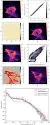 |
Fig. A.5 Same as Fig. A.4, but with a uniform signal-to-noise ratio and different projections. |
| In the text | |
|
Fig. B.1 Comparison of the bin locations for the various sampling options implemented in Colume applied to the column density distribution of the Cha II cloud, with a coarse 50-level sampling, in linear and logarithmic scales. |
| In the text | |
|
Fig. B.2 Effects of sampling options on the global volume density PDF, illustrated by comparing coarse, 50-level volume density reconstructions with a 2000-level benchmark, for the Cha II cloud. |
| In the text | |
|
Fig. B.3 Effects of sampling options on the peak volume density maps, for the Cha II cloud. Top: Peak volume density maps obtained with different coarse, 50-level volume density reconstructions. Bottom: Ratio of these maps to the reference peak volume density map (obtained with a 2000-level i-log percentile sampling). |
| In the text | |
|
Fig. C.1 Variation of anisotropy factor α as a function of scale in the case of Orion A. |
| In the text | |
|
Fig. C.2 Left: Same four panels as Fig. 4, for the Orion A giant molecular cloud. Right: Same, but with anisotropy taken into account. |
| In the text | |
|
Fig. C.3 Left: Comparison of the column density PDF with the global isotropic and anisotropic volume density PDFs derived for Orion A. Right: PDF of the difference between the global volume density distribution derived by the anisotropic and isotropic model (presented on a symmetric logarithmic scale). |
| In the text | |
|
Fig. C.4 Joint distribution of the column density (top) or isotropic peak volume density (bottom) with the difference between the isotropic and anisotropic peak volume densities (left) or their ratio (right). |
| In the text | |
|
Fig. C.5 Comparison of the effect of scale-dependent anisotropy on density maps. From left to right: Column density map used as a prior; peak volume density map obtained with the isotropic model; peak volume density map obtained with the anisotropic model; difference between the two peak volume density maps; ratio between the two peak volume density maps. |
| In the text | |
Current usage metrics show cumulative count of Article Views (full-text article views including HTML views, PDF and ePub downloads, according to the available data) and Abstracts Views on Vision4Press platform.
Data correspond to usage on the plateform after 2015. The current usage metrics is available 48-96 hours after online publication and is updated daily on week days.
Initial download of the metrics may take a while.