| Issue |
A&A
Volume 696, April 2025
|
|
|---|---|---|
| Article Number | A144 | |
| Number of page(s) | 20 | |
| Section | Interstellar and circumstellar matter | |
| DOI | https://doi.org/10.1051/0004-6361/202453409 | |
| Published online | 14 April 2025 | |
Fast spectral line calculations with the escape probability method and tests using synthetic observations of interstellar clouds
Department of Physics,
PO Box 64, 00014, University of Helsinki,
Finland
★ Corresponding author; This email address is being protected from spambots. You need JavaScript enabled to view it.
Received:
12
December
2024
Accepted:
10
March
2025
Abstract
Context. Radiative transfer (RT) effects need to be taken into account when analysing spectral line observations. When the data are not sufficient for detailed modelling, simpler methods are needed. The escape probability formalism (EPF) is one such tool.
Aims. We wish to quantify the model errors in the EPF analysis of interstellar clouds and cores.
Methods. We introduce PEP, a parallel programme for calculating fast EPF parameters quickly. We modelled a full RT to generate synthetic observations for various cloud models. We examined these with the PEP programme, comparing these results to the actual beam-averaged kinetic temperatures, column densities, and volume densities.
Results. PEP enables the calculation of even millions of parameter combinations in a matter of seconds. However, the simple assumptions of EPF can lead to significant errors. In these tests, the errors were typically within a factor of 2, but could (in some cases) rise to one full order of magnitude. The model errors are thus similar or even larger than the statistical errors caused by the typical observational noise. Due to degeneracies, the parameter combinations were shown to be better constrained than the individual parameters. The model errors could be reduced by using full radiative transfer modelling. However, in the absence of full knowledge of the source structure, the errors are difficult to quantify. We also present a method for approximate handling of hyperfine structure lines in EPF calculations.
Conclusions. Both the observational statistical errors and the model errors need to be considered when estimating the reliability of EPF results. Full RT modelling is needed to better understand the true uncertainties.
Key words: line: formation / radiative transfer / methods: numerical / techniques: spectroscopic / ISM: clouds / ISM: molecules
© The Authors 2025
 Open Access article, published by EDP Sciences, under the terms of the Creative Commons Attribution License (https://creativecommons.org/licenses/by/4.0), which permits unrestricted use, distribution, and reproduction in any medium, provided the original work is properly cited.
This article is published in open access under the Subscribe to Open model. This email address is being protected from spambots. You need JavaScript enabled to view it. to support open access publication.
1 Introduction
Radiative transfer (RT) is central to many astrophysics problems from the analysis of observations to the modelling of the thermal balance, ionisation, and chemistry of interstellar clouds. The present paper concentrates on a more limited problem, namely, the role of RT in the direct analysis of spectral line observations. Overall, RT modelling can take into account the assumed threedimensional (3D) distributions of density, velocity, and kinetic temperature, as well as the fractional abundances of the examined species and other sources of radiation and opacity. However, RT is typically treated using some simplifications (Neufeld & Kaufman 1993; Neufeld et al. 1995; Juvela et al. 2003; Peters et al. 2011; Juvela & Ysard 2011; Commerçon et al. 2010; Tomida et al. 2013).
There are many publicly available RT programmes, enabling the estimation of source properties by fitting a source model against the shapes and intensities of the observed lines (e.g. Bernes 1979; Juvela 1997; Harries et al. 2019; Hogerheijde & van der Tak 2000; Dullemond & Turolla 2000; van Zadelhoff et al. 2002; Juvela 2020). However, observations are often insufficient to constrain complex models and faster methods with inherently fewer free parameters would be preferable. The local thermodynamic equilibrium (LTE) approach is the simplest option, providing an analytical mapping between the source parameters and the line intensities. The LTE assumption is sometimes justified, when the level populations can be expected to be close to the LTE values due to high density or high optical depths. However, all sources show some deviations from LTE. For example, due to the decreasing density and increasing probability for the emitted photons to escape, the excitation tends to be lower in the surface layers of molecular clouds. Deviations from LTE become more obvious with better measurements, as the excitation temperatures, Tex, can vary both spatially and between transitions. Therefore, there is a need for methods that are easier and faster than full RT modelling, but that are still able to capture the main effects of non-LTE excitation.
The escape probability formalism (EPF) is one such method (Sobolev 1960; de Jong et al. 1975; Goldreich & Scoville 1976). The source is described by its kinetic temperature, Tkin, column density per velocity interval, dN/dv, and volume density, n. The same values are assumed to apply to the whole source. EPF uses the parameter β to describe the photon escape probability, namely, what fraction of the emitted photons leave the source without being reabsorbed. With assumptions of the source geometry, the parameter β and the local radiation field can be estimated self-consistently with the level populations, thus allowing for deviations from LTE. The escape probability, β, is effectively the same for the whole source but can vary between transitions.
In this paper, we present PEP, a new parallel programme for a EPF analysis of spectral lines. The programme can also be run on graphics processing units (GPUs), with a subsequent potential further speed-up for studies of very large parameter spaces (Tkin, dN/dv, n). We use the programme to analyse far-infrared (FIR) and radio spectral lines for a series of interstellar cloud models. These include spherical clouds and more realistic clumps extracted from a 3D magnetohydrodynamic (MHD) simulation. Sources have strong density variations and the MHD models further spatial variations of velocity, kinetic temperature, and optionally of fractional abundances.
Here, we used 3D non-LTE RT modelling to calculate spectra for several molecules, analyse these synthetic observations with the PEP programme, and compare our results to reference values extracted from the cloud models. The synthetic observations were used without added noise or calibration errors. Our study concentrates on the role of the model errors that result from simplifying the complex 3D objects into a single set of scalar Tkin, n, and dN/dv values. This is complementary to previous studies that have examined the errors resulting from observational noise. Those errors can be estimated locally around the χ2 minimum or preferably analysing the full χ2 space with direct Monte Carlo (e.g. Bron et al. 2018) or Markov chain Monte Carlo (MCMC) methods, or with parameter grids fully covering the relevant 3D parameter space (e.g. Tunnard et al. 2015; Tunnard & Greve 2016; Roueff et al. 2024).
The paper is organised as follows. The EPF methods and the PEP programme are described in Sect. 2. In Sect. 3, the PEP results are compared against calculations performed with the RADEX programme (van der Tak et al. 2007) to confirm their accuracy. To quantify the typical model errors in EPF analysis, we examine in Sect. 4.1 a series of spherically symmetric cloud models. In Sect. 4.2, we consider more realistic observations of inhomogeneous clumps extracted from a 3D MHD cloud simulations. We discuss our findings in Sect. 5, before giving our main conclusions in Sect. 6. One potential way of handling hyperfine structure (HFS) lines in EPF calculations is discussed further in Appendix A.
2 Methods
In EPF the radiation field intensity is a weighted average of the local emission the external background Ibg,
![Mathematical equation: $\[J_\nu=[1-\beta] \Lambda\left(S_\nu\right)+\beta I_{\mathrm{bg}, \nu}.\]$](/articles/aa/full_html/2025/04/aa53409-24/aa53409-24-eq1.png) (1)
(1)
Here, β is the photon escape probability. The local emission is written with the Λ operator that formally operates on the source function, S ν (the ratio of emission and absorption coefficients), the result being that part of J that is caused by emission from the medium. The intensity, Jν, is used to solve level populations ni from the statistical equilibrium equations, each level i having an expression:
![Mathematical equation: $\[n_i \sum_j\left[A_{i j}+B_{i j} J_{i j}+C_{i j}\left(T_{\text {kin }}\right) n^{\prime}\right]=\sum_j n_j\left[A_{j i}+B_{j i} J_{i j}+C_{j i}\left(T_{\text {kin }}\right) n^{\prime}\right] .\]$](/articles/aa/full_html/2025/04/aa53409-24/aa53409-24-eq2.png) (2)
(2)
Here, A represents the Einstein coefficients for spontaneous emission, B the coefficients for stimulated transitions, C the collisional coefficients ([cm3 s−1]), n′ the density of the colliding particles, and Jij the radiation field intensity at the frequency of the transition i → j. The equation is written for arbitrary levels i and j, but spontaneous transitions are possible only to a lower energy level (Aij = 0 for j ≥ i) and radiative transitions (non-zero terms Aij and Bij) are further limited by selection rules. The density n′ and the kinetic temperature Tkin enter the problem via the coefficients C.
The radiation field and the level populations are coupled via the photon escape probability β, which depends on the optical depth of the transition,
![Mathematical equation: $\[\tau_{u l}=\frac{h \nu}{4 \pi}\left[N_l B_{l u}-N_u B_{u l}\right] \phi(\nu) .\]$](/articles/aa/full_html/2025/04/aa53409-24/aa53409-24-eq3.png) (3)
(3)
Indices l and u refer explicitly to the lower and upper energy levels of the transition. Nl and Nu are the corresponding column densities that, in the case of a homogeneous medium, are directly the product of the volume density and the linear source size, s (e.g. Nl = nls). The level population ratios follow the Boltzmann equation,
![Mathematical equation: $\[\frac{n_i}{n_j}=\frac{g_i}{g_j} e^{-\left(E_i-E_j\right) /(k T)},\]$](/articles/aa/full_html/2025/04/aa53409-24/aa53409-24-eq4.png) (4)
(4)
where g represents the statistical weights, E the level energies, and k the Boltzmann constant. In the case of LTE, T would be equal to the kinetic temperature. More generally, the equation defines an excitation temperature Tex that corresponds to the actual level populations.
Overall, EPF gives self-consist values for the optical depths, the escape probabilities β, and the excitation that can now deviate from LTE. For β < 1 the excitation is no longer determined by collisions only, typically resulting in Tex < Tkin. However, EPF assumes a single value of density and kinetic temperature and a single set of level populations for the entire source. The values of β are based on assumptions of the source size and geometry – or, in the case of large velocity gradient (LVG) models, a velocity field that defines a finite source region that can interact via radiation. PEP1 uses the same three alternatives included in RADEX. These correspond to a slab geometry, a homogeneous sphere, and an LVG model (a sphere with constant radial velocity gradient). These result in different expressions for β as the function of optical depth (van der Tak et al. 2007).
The PEP calculations start with LTE level populations at the temperature of Tkin. Together with the other inputs, n and dN/dv, this provides values of optical depth and β for each transition. Instead of explicitly calculating emission via Λ(S), the statistical equilibrium equations are modified by scaling the Einstein coefficients with β. This is the more robust alternative and analogous to the idea of accelerated lambda iterations (Cannon 1973; Rybicki & Hummer 1992). When the level populations are updated, the values of τ and β also change, resulting in new estimates for Jν. The calculations be must iterated until the level populations have converged to their final values. The convergence criterion in PEP is based on the relative changes of the level populations over one iteration. Since convergence slows down at high optical depths, some care is needed in using tolerances that are appropriate for the examined model.
3 Testing of the PEP programme
We compared the PEP results to those calculated with the RADEX programme (van der Tak et al. 2007). Our tests were performed using CO, CS, and HCO+, along with their isotopomers, as well as the rotational spectrum of p-H2O. The molecular data were taken from the LAMDA database (Schöier et al. 2005).
Figure 1 shows examples of results for the first seven transitions of CO, HCO+, and p-H2O (noting that the first transitions here indicate the transitions between the lowest J levels). The models cover a range of optical depths from optically thin to optically very thick. The relative populations of the J = 7 level are ~10−7, and after J = 7–6 the transitions have TR < 1 μK, values far below the detection threshold of typical observations. The match between the PEP and RADEX results is good, both in this case using β values for the LVG case.
For the calculations of a single set of parameters RADEX is faster, but PEP is more efficient when results are needed for tens of parameter combinations. The difference becomes significant for large parameter grids, potentially more so if calculations can be done on a GPU with single-precision floating point arithmetic (Appendix B). Figure 1 also shows results for a non-parallel, double-precision Python version. Figure 2 shows the populations for the 22 lowest energy levels in a Tkin = 70 K model. The single-precision results deviate by several percent after J ~ 15, where the relative populations are however already below 10−8. The accuracy of single-precision calculations thus appears to be sufficiently for most applications. The PEP parallel and non-parallel runs with double precision give the same results, and also differences to RADEX remain insignificant, reaching ~10% at the highest level where the relative populations are only ~10−14.
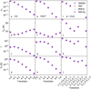 |
Fig. 1 PEP and RADEX results for density n(H2) = 103 cm−3, column density of the species N = 1015 cm−2, and a 1 km s−1 linewidth. The temperature is Tkin = 20 K for the CO (left frames), Tkin = 10 K for the HCO+(middle frames), and Tkin = 100 K for the H2O (right frames) runs. The plots show the fractional upper level population nu, excitation temperature Tex, optical depth τ, and the radiation temperature TR for the first seven transitions. PEP results are shown for single-precision (PEP) and double-precision (PEP-D) runs and for a pure Python implementation without parallelisation (“PEP-Py”). |
4 Results
We used non-LTE RT runs to produce spectra for different cloud models, analysed these synthetic observations with PEP, and compared the results to the known values of the model clouds. The synthetic spectra were made with the RT programme LOC (Juvela 2020). Section 4.1 examines spherically symmetric models that cover a wide range of optical depths and have non-uniform radial density profiles and partly non-uniform temperatures. In Sect. 4.2 we analyse spectra of more realistic clumps extracted from an MHD simulation of star-forming clouds with supernova-driven turbulence. We use in the tests seven molecular species with the default fractional abundances χ of 10−4 for CO, 2 × 10⁻⁶ for 13CO, 3 × 10⁻⁷ for C18O, 2 × 10⁻⁹ for HCO+, 8 × 10⁻¹¹ for H13CO+, 5 × 10⁻⁹ for CS, 10−10 for C34S, and 10−9 for N2H+ (see Navarro-Almaida et al. 2020 and references in Juvela et al. 2022). N2H+ is only used in separate tests of the HFS calculations. EPF provides direct column density estimates only for the analysed species. However, to facilitate comparisons between molecules and especially in cases of joint analysis of different species, the results are plotted as functions of N(H2), using the true values of the fractional abundances, χ.
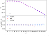 |
Fig. 2 CO level populations for Tkin = 70 K, n(H2) = 104 cm−3, N(CO) = 1018 cm−2, and FWHM = 1 km s−1. The upper frame shows the level populations for all 22 levels (J = 0–21), and the lower frame shows the level populations relative to the double-precision PEP calculations. |
4.1 Test with spherically symmetric cloud models
4.1.1 Isothermal models
Our tests were conducted with spherically symmetric cloud models. We note that even when density and Tkin are constant, the excitation will vary radially. This is in contradiction with the EPF assumptions, while the radial density and Tkin gradients can further affect the accuracy of the EPF analysis. We first examined isothermal clouds, where the density profiles correspond to critically stable Bonnor-Ebert (BE) spheres (Ebert 1955; Bonnor 1956) with no large-scale velocity field.
Figure 3 shows an example of the actual photon escape probabilities, excitation temperatures, and line intensities calculated with the LOC programme. The cloud is a Tkin = 10 K BE sphere with a mass of 10 M⊙. The 12CO lines have high optical depths with peak values of 29.4, 49.6, and 26.7 for J = 1–0, J = 2–1, and J = 3–2, respectively. The radial variation of Tex is a factor of 2, while the escape probability increases from close to zero at the centre to β ≳ 0.5 on the cloud surface. EPF cannot be expected to be accurate for models of such high optical depths, but some degree of Tex and β gradients exist in all models.
We calculated synthetic spectra towards the model centre, convolved with a Gaussian beam with FWHM equal to one-third of the cloud radius, FWHM = R0/3. These ‘observed’ spectra were fitted with Gaussians and the EPF analysis was based on the fitted intensities. Initially, Tkin was fixed to its correct value. Then, EPF gives predictions for the density and the column density, when dN/dv is converted to column density using the correct line FWHM. The beam-averaged reference values of column density and volume density values were obtained directly from the model cloud. In the line-of-sight (LOS) direction, these include the full model volume up to the surface of the BE sphere.
The PEP calculations were performed for a wide range of densities and column densities around the reference values. For example, the high optical depth of 12CO lines of the M = 2 M⊙ and Tkin = 10 K model resulted in a highly degenerate solution, which was not in contradiction with the reference values, but also provided no upper limits for density and column density. The corresponding results for 13CO are shown in Fig. 4. Each transition constrains the EPF solution to a band of parameter values, the green hatched region showing the area where the line intensity predicted by PEP is within ±10% of the observed line intensity. The n(H2) values are not constrained but the EPF analysis is mostly consistent with the reference values of density and column density. The combination of the multiple transitions provides more constraints, but for example the combination of J = 1–0 and J = 4–3 would only reject densities above the n(H2) reference value.
The above 12CO and 13CO spectra were not optically thin and were either flat-topped or with self-absorption dips (see Appendix C.1). The CS and C34S results for the same cloud model are shown in Fig. 5. The CS J = 2–1 spectrum has a small dip in the line centre, but the other spectra are nearly Gaussian. The predicted bands of n(H2) and column density are narrow, especially for C34S. They are partly inconsistent with each other (e.g. CS J = 3–2 vs. J = 5–4), but for example the combination of C34S J = 2–1 and J = 5–4 would constrain the solution close to the reference solution.
Corresponding results for 12CO and 13CO spectra from the 10 M⊙ cloud at Tkin = 20 K are shown in Appendix C.1 (Fig. C.6). This shows similarly some some discrepancy between the isotopomers, even with perfect knowledge of the fractional abundances. For example, the combination of 13CO J = 1–0 and J = 4–3 lines would result in a nearly unique solution but with ~0.2 dex errors, underestimating the n(H2) and overestimating column density. Of other combinations, CO(3-2) and 13CO(1–0) would indicate that the density is too low by at least 0.5 dex and the column density is too high by the same factor.
We examined the χ2 values for combinations of multiple transitions, using BE models with masses of M = 0.2, 5, and 10 M⊙ and kinetic temperatures of Tkin = 10, 20, and 50 K. The observations are assumed to have 10% uncertainty, but no noise was added to the input spectra. The fit quality was measured by a χ2 value that is the average of the individual transitions. For observations with 10% noise, χ2 would thus be expected to be of the order of 1.
The value of Tkin was initially fixed to its correct value. Figure 6 shows χ2 values for 13CO. To resolve the χ2 minimum, the number of data points was 300 along both the density and column density axes. The addition of a second transition partly breaks the degeneracy, but further transitions provide only little improvement. The χ2 minimum is slightly above the correct N(H2) value but almost 0.5 dex below the reference density. The dense part of the cloud emits more strongly, especially if outer parts fall below the critical density. Therefore, one might expect EPF to overestimate the reference density. However, this is not what is seen in Fig. 6.
Figure 7 summarises the results for seven molecules in the case of the M = 0.5M⊙ and Tkin = 20 K model. The χ2 values are in some cases much higher at the location of the reference parameters n(H2) and N(H2) than at the χ2 minimum (e.g. for C34S and H13CO+). The EPF analysis would thus reject the correct solution with an apparent high level of confidence (if the reference solution can be considered the correct one). Even the minimum χ2 values can be high, up to χ2 ~ 100, when the evidence of the individual transitions is contradictory. The previous figures already showed (e.g. Fig. 5) that χ2 can increase very rapidly when one moves outside the narrow valley of the lowest χ2 values.
Figure 7 shows that in most cases the column density is correct to within a factor of a few. The main exception is HCO+. Based on the spectral profiles shown in Appendix C.1, this could be due to strong self-absorption. Although Fig. 7 suggest order of magnitude errors for HCO+, the high optical depth also means a larger degree of degeneracy, where the global χ2 minimum can be located far from the reference parameter values, the latter still not being rejected with any high significance. Indeed, for HCO+the χ2 values are almost the same at the reference position, indicating that the parameters are not well constrained. The same applies to 12CO and 13CO, although there the nominal parameter uncertainties tend to be smaller. While EPF cannot be expected to be accurate for optically thick lines, the same applies to some extent to any RT analysis (van der Tak et al. 2007; Asensio Ramos & Elitzur 2018). For the less optically thick species, the column density may be correct to within a factor of 2; however, as implied by previous χ2 images, the density remains unconstrained. Appendix C.2 includes further plots for other cloud models, where a higher Tkin tends to result in more accurate results.
Figure 8 shows an example where 13CO spectra are analysed using Tkin that is 30% below or above the correct value. Depending on the transitions used, this uncertainty on Tkin can result in a change in the estimated density of up to 1 dex. In this example, the 30% underestimation of Tkin actually gives partly the best match to reference n(H2) and N(H2) values. Higher Tkin values decrease the estimated N(H2) to slightly less than 0.5 dex for the ±30% Tkin change.
Figure 9 shows results for the same model, varying Tkin around the correct value. The χ2(Tkin) does not have a clear minimum; however, the estimated column density remains correct to within a factor of 2 over the plotted range, with only a slightly larger maximum error (and negative bias) for the density.
The situation is very different for the denser cloud with M = 2 M⊙ (Fig. 10). The χ2(Tkin) reaches the minimum ~2 K above the true temperature, at which point N is correct to within a factor of 2, but the density is poorly constrained. As Tkin increases, the n(H2) estimate drifts from the upper limit to the bottom limit of the probed range. This reflects the almost completely degeneracy of the models with respect to n(H2). If the temperature were fixed to the correct value of Tkin = 20 K, the column density would be strongly overestimated, as suggested by Fig. 7. The plot of the χ2 planes are included in Fig. C.11. That shows that, apart from the +30% Tkin value, the spectra are at the limit of saturation, which results in the observed large errors.
A more positive example C34S spectra is shown in Fig. 11, where the χ2 minimum is reached at the correct temperature, with accurate predictions for both n(H2) and the column density. However, even in this case, if Tkin were fixed to just 1 K higher value, the errors could approach one order of magnitude.
In the above tests the ±30% range of Tkin was sampled with 100 points (e.g. ΔTkin = 0.025 K for Tkin = 10 K). Given the reference values for n(H2) and N(H2), our PEP calculations covered parameter ranges from 50 times lower to 50 times higher values, using a grid of 500 × 500 points. Despite the fine grid, the aliasing is still visible as saw-tooth pattern, especially in Fig. 11. This could be avoided by interpolation, but is shown as a reminder of the parameter degeneracies and the resulting challenging shape of the χ2 surface.
When the analysis includes multiple species, the results depend on the assumed fractional abundances. Figure 12 shows an example of the combination of CS and C34S observations with ±50% errors in the assumed C34S abundance. Density is constrained only if higher transitions are included. The changes in the fractional abundance cause a 0.5 dex shift in the column density, an effect that is more significant than the direct error in the C34S abundance. Appendix C.2 shows further examples for the same lines at Tkin = 10 K or Tkin = 20 K, generally with similarly minor effects on the parameter estimates.
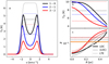 |
Fig. 3 Example of optically thick CO emission from a 10 M⊙ BE model with Tkin = 10 K. Frame a shows spectra, frame b Tex profiles, and frame c the radial variation in the photon escape probability β. Results are shown for full non-LTE calculations with LOC (solid lines), for constant excitation equal to the mean values of the LOC solution (“⟨LOC⟩”, dashed lines), and for the LTE case at Tkin (dotted lines). Frames a–b show data for the first three transitions (black, blue, and red, respectively) but, for clarity, frame c includes only the J = 1–0 and J = 3–2 transitions. |
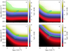 |
Fig. 4 PEP results for 13CO spectra towards a BE sphere with Tkin = 10 K and M = 2 M⊙. The colour scale shows the predicted line intensities as a function of volume and column density. In the green hatched areas PEP predictions are within 10% of the observed line intensities. The circles indicate the reference cloud parameters for the central LOS (small circle), along with the beam average with FWHM = R0/3 (middle circle corresponding to the beam in the synthetic observations) and for FWHM = R0 (large circle). |
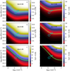 |
Fig. 5 PEP analysis of CS (left frames) and C34S (right) line intensities. The plotted symbols are as in the previous figures. The cloud model is the same as in the previous figures, with M = 2 M⊙ and Tkin = 20 K. Each frame quotes the depth of the possible self-absorption dip as the line intensity at the line centre divided by the maximum intensity. |
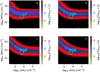 |
Fig. 6 Combined χ2 values in PEP analysis of 13CO spectra. The cloud model an isothermal BE sphere with M = 10 M⊙ and Tkin = 20 K. The frames a-d correspond, respectively, to the combinations of the 1–4 first rotational transitions. The circles indicate the reference values towards its centre (smallest circle), averaged over a FWHM = R0/3 beam (middle circle that corresponds to the synthetic observations), and averaged over a FWHM = R0 beam (largest circle). |
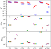 |
Fig. 7 Results for seven molecules observed towards an isothermal BE sphere with M = 0.5 M⊙ and Tkin = 20 K. Frame a shows the minimum χ2 value (blue open circles) and χ2 value for the reference density and column density (red filled circles). Frames b and c, respectively, show the ratio of density and column density values at the χ2 minimum relative to the reference values. Each molecule is plotted with four markers that, from left to right, correspond to the combination of the lowest transitions (1–4). |
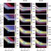 |
Fig. 8 Plots of χ2 in the EPF analysis of 13CO lines. The analysis used three Tkin temperatures, as listed above each column of frames. The cloud model is an isothermal BE sphere with M = 10 M⊙ and Tkin = 20 K. First row shows the analysis of the J = 1 − 0 lines, and each subsequent row adds one further rotational transition. The contours are drawn at χ2 levels of 1 (red), 2 (cyan), 10 (magenta), and 100 (blue contour). In order of increasing size, the circles indicate the reference density and column density values towards the model centre, averaged over a FWHM = R0/3 beam (used for the synthetic observations), and averaged over a FWHM = R0 beam. |
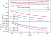 |
Fig. 9 Change in the minimum-χ2 PEP solution for 13CO spectra as a function of Tkin. The model is a 10 M⊙ BE sphere with Tkin = 20 K. Frame a shows the minimum value of χ2 (solid lines) and the χ2 value for the reference parameter values (dashed lines). Frame b shows the predicted density and frame c the predicted column density. The cyan, magenta, and red colours correspond, respectively, to the analysis using two, three, or four transitions. |
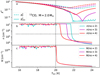 |
Fig. 10 Same as Fig. 9, but for the synthetic 13CO observations of the M = 2 M⊙ and Tkin = 20 K model. |
4.1.2 Non-isothermal models
As the final exercise with the 1D models, we examined the effect of radial Tkin gradients. The mass-weighted mean Tkin was set to 10, 20, or 50 K, and the density profile was calculate for the corresponding isothermal model. The temperatures were then modified to have a constant positive or negative gradient. The total temperature variation is 30% of ⟨Tkin⟩, but the mass-weighted average temperature ⟨Tkin⟩ was kept at the original value.
Figure 13 shows results for 13CO spectra from a model with Tkin increasing outwards, for observations with a Gaussian beam of FWHM = R0/3. Apart from the temperature gradient, the situation is the same as in Sect. 4.1.1. The line intensities predict column densities that are below the reference value, although the change is less than 0.2 dex. The case with Tkin decreasing outwards is shown in Fig. 14. The 13CO J = 1–0 transition is now matched over a much wider range of parameters, while higher transitions now prefer column density that is 0.2 dex above the reference value (at the same density) or 0.4 dex above the previous case with Tkin increasing outwards.
Appendix C.3 shows two further examples with radial Tkin gradients for the combination of CS and C34S spectra. Overall, the temperature gradients introduce only modest changes compared to the isothermal cases.
Figures 15 and 16 show a more extreme example, namely, of the 12CO observations of the M = 2 M⊙ model with Tkin = 10 K. As explained in Appendix C.1, the corresponding 12CO spectra of isothermal models are flat-topped but do not yet show any self-absorption dips. However, when Tkin increases outwards (Fig. 15), the observations fall in the saturated region, and only the optically less thick J = 4–3 transition is able to constrain the combination of density and column density values. When the temperature gradient is reversed (Fig. 16), the results have the appearance of n(H2) and the column density being better constrained but the values are in reality significantly underestimated.
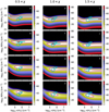 |
Fig. 12 Estimated χ2 for combined CS and C34S observations of a BE sphere with M = 0.5 M⊙ and Tkin = 10 K. The columns correspond to the assumed C34S abundances (correct and with ±50% errors). The first row shows results for the J = 1 − 0 line, and each subsequent row adds one more rotational transition. |
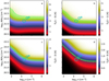 |
Fig. 13 Results for 13CO spectra of the M = 2 M⊙ BE model with ⟨Tkin⟩ = 10 K. The case is similar to that of Fig. 4, except that Tkin increases outwards. |
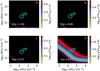 |
Fig. 15 Values of χ2 as function of density and column density for a non-isothermal 2M⊙ model with ⟨Tkin⟩ = 10 K and Tkin increasing outwards. Frame a is based on the fit to 12CO J = 1–0 spectra, and each subsequent frame includes to the analysis one further rotational level. |
4.2 Clumps from 3D MHD cloud simulation
As more realistic examples of sources, we examined clumps extracted from a (250 pc)3 MHD simulation of supernova-driven turbulence (Padoan et al. 2016). The mean density of hydrogen nuclei in the model is 5 cm−3, but turbulence and self-gravity increase the maximum values to ~107 cm−3 in the selected snapshot. The hierarchical discretisation reaches a maximum resolution of 7.6 mpc.
The simulation provides the density and velocity fields. The velocity dispersion inside the cells was estimated from the dispersion between neighbouring cells (23 cells per octree parent cells, scaled down by a factor 1.5) and this is added to the thermal line broadening. Because the MHD simulation does not provide gas kinetic temperatures Tkin, we used dust temperatures from separate continuum RT calculations (see Juvela et al. 2022) as the proxy for Tkin. Gas temperature follows dust temperature accurately only at densities n(H2) ≳ 105 cm−3 (Goldsmith 2001; Juvela & Ysard 2011). However, the procedure gives a realistic temperature structure that extends from typical ~20 K at low densities to less than 10 K in dense cores. The continuum modelling includes radiation of the stars that have formed in the MHD simulation. This increases further the complexity of the temperature field, 0.25% of the cells reaching values above Tkin ~30 K.
In the absence of chemical modelling, we used constant factional abundances or, alternatively, values further set based on the density, χ = n(H2)2.45/[3.0 × 108 + n(H2)2.45]χ0, with the χ0 values listed at the beginning of Sect. 4. The abundance becomes small below n(H2) ~ 2 × 103 cm−3, thus affecting more lines of low critical density (Shirley 2015).
We calculated 13CO spectral line maps for the full MHD model, convolved the line area map to 0.25 pc resolution, and selected peaks with the integrated J = 2–1 line intensity above 6 K km s−1. For each peak, we located the maximum volume density along the line of sight, and resampled the data for the surrounding (7.9 pc)3 volume onto a Cartesian grid with a 0.061 pc cell size. After rejecting sources close to the edges of the MHD cube and three sources with multiple velocity components, the final sample contains 55 targets that are in the following called clumps.
The LOC programme was used to calculate synthetic non-LTE spectra for 12CO, 13CO, C18O, CS, C34S, HCO+, and H13CO+, using the first three rotational transitions for the EPF analysis. Each clump was observed with the beam sizes of FWHM = 0.31, 0.61, and 1.22 parsecs (5, 10, or 20 model cells), and the parameters of Gaussians fits to the line profiles were used as inputs for the EPF analysis.
We extracted reference values from the model cubes. The mean densities and mean column densities were obtained by weighting the data with the same Gaussian beams as in the synthetic observations. The mean temperature ⟨Tkin⟩ was weighted by both the beam and the density. When the fractional abundances were not constant, alternative values of ⟨n(H2)⟩, ⟨N(H2)⟩, and ⟨Tkin⟩ were obtained by further weighting the data by the fractional abundances. A large part of each model cube is filled by low-density gas will small contribution to the emission. Therefore, in the constant-abundance case the reference density can be expected to be lower than the mean density derived from the observed spectra. The difference should be smaller in the case of variable abundances, because the abundance weighting also reduces the contribution of low-density cells with n(H2) ≲ 103 cm−3.
Figure 17 shows 13CO(2–1) maps for one clump and different beam sizes. The field shows a typical filamentary structure that, when observed with a large beam (e.g. FWHM = 0.61 pc or FWHM = 1.22 pc), can lead to low beam filling. We analyse for each clump only one line of sight that corresponds to the maximum of the 13CO J = 2–1 line area map observed with the FWHM = 0.31 pc beam.
Figure 18 shows results for one clump with constant fractional abundances and the intermediate beam size. The EPF analysis uses a kinetic temperature equal to ⟨Tkin⟩. The χ2 values are averages over the first three rotational transitions and are shown for 12CO, 13CO, CS, C34S, HCO+, and H13CO+. The beam-weighted reference values ⟨n(H2)⟩ and ⟨N(H2)⟩ are also shown.
The EPF estimates of the density and column density are still strongly degenerate. Only 13CO results show a clear localised minimum, although more than an order of magnitude above the expected density ⟨n(H2)⟩. That is caused by the reference value of ⟨n(H2)⟩ including low-density gas with little contribution to the observed spectra. Even if the reference value were an order of magnitude higher, to match the predicted volume density, the column density would still be overestimated by almost 0.5 dex. That density would be almost 1 dex above the EPF prediction based on the 12CO lines. A 20% change in the assumed Tkin would change these results only marginally.
In the variable-abundance case the reference value for n(H2) is indeed about one order of magnitude higher (Fig. 19), in better agreement with the EPF predictions based on the 13CO lines. However, the reference values are still at ~0.3 dex lower density and ~0.2 dex higher column density. For 12CO the reference values are clearly above the EPF predictions, which show a narrow valley of low χ2 values. For the other molecules the reference values are located only very slightly below the χ2 valley.
The plots show very elongated regions of low χ2 values. Therefore, instead of the difference between the reference parameter values rref and the χ2 minimum of EPF estimates, we concentrate on the distance between rref and the nearest point along the χ2 valley. We searched the minimum ![Mathematical equation: $\[\chi_{\text {line }}^{2}\]$](/articles/aa/full_html/2025/04/aa53409-24/aa53409-24-eq5.png) along the (Δ log n(H2), Δ log N(H2)) = (1,1) direction. That was subsequently replaced with the final position, rest, which is the closest position to rref, where
along the (Δ log n(H2), Δ log N(H2)) = (1,1) direction. That was subsequently replaced with the final position, rest, which is the closest position to rref, where ![Mathematical equation: $\[\chi^{2} \leq \chi_{\text {line }}^{2}\]$](/articles/aa/full_html/2025/04/aa53409-24/aa53409-24-eq6.png) , and all distances are measured in terms of density and column density logarithms. The distance between rref and rest is thus only a lower limit for the distance between rref and the global χ2 minimum. When χ2 varies little along the χ2 valley, it is still a good measure for the discrepancy between the EPF predictions and the reference values.
, and all distances are measured in terms of density and column density logarithms. The distance between rref and rest is thus only a lower limit for the distance between rref and the global χ2 minimum. When χ2 varies little along the χ2 valley, it is still a good measure for the discrepancy between the EPF predictions and the reference values.
Figure 20 shows the density and column density ratios between the rref and rest positions, using the notation Nest/Nref = N(rest)/N(rref). The data consist of 12CO observations with the FWHM = 0.61 pc beam size. The reference values rref are again averages from the model cubes weighted by the beam and, in the case of varying abundances, also by the abundance χ.
As suggested by Fig. 18, in the case of 12CO the bias is not very large even in the constant-abundance case, with 0.3 ≲ nest/nref ≲ 1.6 and 0.2 ≲ Nest/Nref ≲ 1.5. One should also remember that the best definition of the reference density remains uncertain. In the variable-χ case the EPF analysis of 12CO underestimates the reference values typically by a factor of 2, in agreement with Fig. 19.
We also analysed 12CO observations for models, where the densities were increased by an ad hoc factor of 5 (figures not shown). The results are qualitatively similar to Fig. 20, except that for seven cores the 12CO line intensities fall into a degenerate region due to line saturation. Thus, instead of the one outlier in Fig. 20, there are now more outliers with high n(H2) and N(H2) values (seven for constant-χ and 14 for the variable-χ case). In those cases the global χ2 minimum may be located at much higher n(H2) and N(H2) values but χ2 being only slightly lower than at the rref position. Thus, in the case of these outliers, EPF is not able to constrain the parameters but also is not in strong contradiction with the reference values.
The results for 13CO spectra are shown in Fig. 21. For constant fractional abundances, the n(H2) and N(H2) estimates are ~30% above the reference values, and the largest discrepancies exceed a factor of 2. In the case of variable χ, the reference values are underestimated, especially in column density. Figure 21b contains one outlier where the n(H2) and column density ratios are exceptionally low. The source appears normal, except for its low temperature: ⟨Tkin⟩ = 9.6 K. If the model densities were increased by a factor of 5 (not shown), there are no outliers. The 13CO parameter estimates are closer to the reference values in the constant-χ case, while in the variable-χ case column density estimates are on average 45% of the reference values.
In addition, other molecules tend to show larger discrepancy in the constant-χ case, partly because the reference value of n(H2) underestimates the density of the emitting (sub)region (Appendix D). The variable-χ results are consistent with the reference values to within a factor of 2, with occasional outliers. The main feature is the correlation between the density and column density discrepancies (distance between rest and rref). This is not caused directly by our definition of rest, which could be located in any direction from rref, as long as its χ2 values is equal or smaller than the minimum value along the initial diagonal search direction.
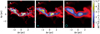 |
Fig. 17 Example of a clump extracted from the MHD model. The frames show the 13CO(2-1) line-area maps at the full resolution (frame a) and for observations with FWHM = 0.31 pc (frame b) and FWHM = 0.61 pc (frame c) beam sizes. The fractional abundance is spatially constant. |
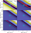 |
Fig. 18 PEP results for a MHD clump, using the Tkin value given in frame a. Each frame shows χ2 for one molecule and its first three rotational transitions. The cyan circles indicate the beam-averaged model mean densities and column densities (sizes in order of increasing FWHM). The χ2 values are based on the medium beam size. The blue, cyan, magenta, and red contours correspond to χ2 = 1, 2, 10, and 100. |
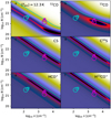 |
Fig. 19 Same as Fig. 18 but for a model with density-dependent abundances. The reference values are shown without (cyan circles) and with the weighting by fractional abundances (magenta circles). The circle sizes correspond to the three beam sizes, in order of increasing FWHM. The χ2 values correspond to observations with the intermediate beam size. |
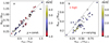 |
Fig. 20 Comparison of EPF estimates and reference values for 12CO spectra observed with the intermediate beam size. Frames a and b correspond, respectively, to the constant and variable abundance cases. The marker colours show the χ2 ratio between the rref and rest positions. In frame b, the red text refers to one outlier with ratios greater than 10. |
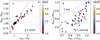 |
Fig. 21 Same as Fig. 20 but for the 13CO observations. Blue text in frame b refers to one outlier with both ratios below 0.05. |
5 Discussion
We present PEP, a parallel programme for EPF line calculations. Synthetic spectral line observations were used to investigate the differences between the EPF predictions and the actual source parameters. The parameters, pi, span the volume density, n(H2), the column density, N, of the examined species (together with the assumed line width FWHM), and the kinetic temperature, Tkin. We have omitted observational errors and concentrated on the model errors caused by the assumptions inherent to the EPF analysis.
5.1 Spherically symmetric models
The spherically symmetric 1D models break the EPF assumptions due to radial variations in the photon escape probability (see Fig. 3), the effects being enhanced by non-uniform density and Tkin. For optically thick lines, these lead to self-absorption that cannot be modelled with EPF and usually results in biased results or little constraints on the source parameters. Even in the absence of strong self absorption, each line probes preferentially different cloud layers, according to its optical depth.
To constrain all parameters, pi, it is, in principle, better to combine observations of lines with different (lower) optical depths and critical densities (Tunnard & Greve 2016; Roueff et al. 2024). In the tests the degeneracy was sometimes reduced by combining multiple transitions of the same species, such as the case of C34S in Fig. 5. However, it was also seen that different transitions may not all be consistent with the same solution (e.g. 13CO in Fig. C.6). Combined with parameter degeneracies, this can result in an apparent match with observations but with clearly erroneous parameter values. When observations of different species are combined, incorrect estimates of the fractional abundances clearly bias the results or, if that uncertainty is taken into account, will weaken the constraints on the cloud parameters.
The reference values of mean density and column density were relatively well defined, thanks to the clear outer boundary of the BE spheres. In tests with the correct Tkin values, the combination of n(H2) and N(H2) (in plots corresponding to the true fractional abundance of the species) was generally constrained to a narrow band, and the individual parameters could not be determined with high accuracy (such as in the tests conducted with the 12CO and 13CO lines). When lines were not optically thick, the column density estimates (at the χ2 minimum) were mostly within a factor of 2 of the correct value (Fig. 7 and Figs. C.7–C.10). However, also much larger errors can occur and even at moderate optical depths.
When temperature was included as a free parameter, correct values of Tkin, n(H2), and column density could be recovered accurately only in the best cases. The examples showed that a 1 K error in Tkin could result in changes in the other parameters up to a factor of a few (Fig. 11). The tests did not include observational noise, but those large errors might well be realised due to noise in intensity measurements. For the optically thicker 13CO lines, the Tkin estimates were generally biased or Tkin remained unconstrained. In some cases, the n(H2) and column density estimates were quite insensitive to temperature (Fig. 9). In other cases, especially due to line saturation, an error in temperature of less than one degree could result in a change in the other predicted parameters up to an order of magnitude (Fig. 10). The analysis of multiple species and transitions of different optical depths should either confirm the correct solution or reveal the true uncertainty of the estimates.
5.2 Clumps extracted from MHD simulations
The MHD simulation provided more realistic test cases with complex density and temperature structures and the added effects of different velocity fields and optional abundance variations. The model complexity also makes it more difficult to define the reference solution (the ‘true’ parameter values), because emission often originates in some model sub-volume. The reference solutions were more likely to be more accurate in the variable-abundance case, when nref = ⟨n(H2)⟩ and Nref = ⟨n(H2)⟩ were weighted not only by the beam but also by the density-dependent abundances, thus eliminating the low-density gas from these averages.
The EPF estimates of nest and Nest were for individual transitions again mainly limited to narrow bands. Therefore, we calculated only distances between the reference value rref and the closest EPF solution point rest with χ2 values similar to the closest position along the χ2 valley. The discrepancy between the two parameter positions typically showed a factor of 2 in scatter, the density and column density being both either overestimated or underestimated. This results from the actual anticorrelation between n(H2) and column density. One could of course reach the χ2 valley also by moving along just one parameter axis, assuming no error in one parameter and larger error in the other. The selected shortest distance results in the discrepancy being attributed roughly equally between n(H2) and N(H2) (on logarithmic scale).
In several examples, the constant-χ EPF estimates were unbiased or even (on average) larger than the reference values. In the variable-χ case the predictions were mostly lower, especially for the column density. The systematic errors could be even more than a factor of 2 and individual clumps showed additionally more than a factor of 2 in the scatter in the Nest/Nref ratio around the biased mean. The mean error and the scatter of the predicted density were smaller. Overall, the model errors often cause a discrepancy between the EPF estimates and the reference values that is more than a factor of 2.
The above discrepancy (e.g. Nest vs. Nref) is only a lower limit for the formal error, since the global χ2 minimum could be located even much further. Figure 22 is similar to Fig. 21 but uses the χ2 minimum instead of rest to characterise the errors in the EPF analysis of 13CO spectra. The bias in the column density values has grown to about a factor of 3, and in the variable-χ case the density is now overestimated by a factor of ~2.5.
The model errors are thus an important source of uncertainty in the EPF analysis. They can be larger than the uncertainty of typical observational errors, which previous studies have shown to be typically of the order of a factor of 2, of course depending on the used lines and the signal-to-noise ratios (Roueff et al. 2024).
Figure 23 shows an example of the effect of observational noise in the analysis of 13CO spectra from one of the MHD clumps. The frames show χ2 for five Tkin values around the estimated ⟨T(kin)⟩. The χ2 values are averages over the first three transitions, assuming 20% error estimates for the line intensities. In this case NEPF is underestimated by ~0.3 dex, and the best match with the expected density values is reached for 20% higher Tkin. However, Tkin is not well constrained, because the minimum χ2 decreases towards higher Tkin, where density becomes underestimated. The white dots correspond to the χ2 minima for 50 realisations of line intensities according with the assumed 20% observational noise. The points are distributed over the χ2 minimum of the noiseless observations. In this case the model errors cause bias (shift relative to the expected parameter values, including the Tkin dependence) that is of the same order of magnitude as the scatter caused by the statistical observational errors. If the observational errors were smaller, the errors would thus be dominated by the model errors.
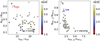 |
Fig. 22 Same as Fig. 21, but using estimates from the global χ2 minimum instead of the closest position rest along the χ2 valley. |
5.3 Comparison of EPF and full RT modelling
The EPF analysis could be replaced with full non-LTE RT modelling. This would result in significant increase in computational cost, but could be justified if the results were more accurate.
We examine briefly the example of a M = 2 M⊙, Tkin = 15 K BE model, using the first three transitions of CS and C34S. Figure 24a shows the general 3D shape of the χ2 surface in the EPF fits. We made corresponding calculations with the LOC programme, using a grid of cloud models that resulted from direct scaling of the correct cloud model to other densities, column densities, and temperatures. Since this grid includes the model that produced the synthetic observations, the minimum χ2 value is in this case zero. The overall χ2 distribution (Fig. 24b) is observed to be only roughly similar to that of the PEP calculations. In the EPF calculations, the minimum χ2 is however found at very low temperature (below 7 K), where the column density is underestimated by 40% and the volume density by a factor of 4. If the temperature is fixed to the correct value (Tkin = 15 K), the column density is still underestimated by a factor of 2, while the density is now overestimated by less than 40% (Figs. 24c and d). Overall, in LOC results the χ2 minimum is better localised and, as it is based on the correct cloud model, is also unbiased (Fig. 24d).
In the case of real observations, cloud modelling certainly has to be done with more limited knowledge of the real source structure. The use of a more realistic density profile (instead of the EPF single-point estimates) should result in some improvements, although it will be difficult to predict how this is reflected in the n(H2) and column density accuracy. We made one test using the observations of the above BE model (M = 2M⊙, Tkin = 15 K). We calculated a grid of RT models where the radial density distributions were Gaussian instead of the correct BE profiles. The χ2 minimum of the Gaussian models was found at 12.7 K, with column density 30% and volume density just a couple of per cent above the correct value. Although the values are not exactly correct, this is still a significant improvement over the previous EPF results. If Tkin is fixed to 15 K, the relative improvement over EPF is smaller but still significant, with the full RT model overestimating the column density by 25% and underestimating n(H2) by 10%.
This is only an isolated example based on the comparison of the χ2 minima, without considering the full χ2 surfaces. Furthermore, in a non-uniform cloud the correct values of n(H2) and the column density are still subject to some interpretation. In the above test the Gaussian density profiles were rather similar to the actual BE profiles. If the approximation of the cloud structure were less accurate, also the improvement over the simpler EPF analysis would be more limited.
Full 3D RT calculations are still needed, if one wishes to match the observed line shapes (regarding the kinematics and the optical-depth effects), examine abundance variations (e.g. in connection with chemical models), combine observations that are clearly probing different parts of the object, or generally whenever deviations from homogeneity become evident in the observed data. Synthetic observations based on specific cloud models or simulations should of course also be preferentially based on full non-LTE RT calculations.
5.4 Implementation of the PEP programme
In the test cases (Sect. 3), PEP reproduced accurately the results calculated with the RADEX programme (van der Tak et al. 2007). In single-precision calculations differences appeared only for levels with populations ~10−8, which are not likely to be important in real observations. This should enable faster calculations on GPUs. Calculations for ~105 density and column density combinations could be computed within about one second. This makes it possible to do the calculation on-the-fly, as diagnostic plots are made. However, for grids of moderate sizes (e.g. 100 × 100 grid points), the run times were similar on both CPUs and GPUs (Appendix B). Therefore, there is generally no need to use a GPU, although that may still provide some speed-up in larger parameter studies (Fig. B.1).
In PEP the parallelisation is done over the density and column density values, using collisional coefficients precomputed for the chosen Tkin. Three-dimensional grids (n, N, Tkin) are still processed efficiently with a simple loop over temperature, especially since the Tkin grids tend to require fewer points. Full coverage of the relevant 3D parameter space (possibly combined with some priors) also makes it possible to quantify the formal uncertainties. Since the problem involves at most three parameters, this is faster than the use of for example MCMC methods. On the other hand, as shown in this paper, the model errors can be a significant or even the dominant source of uncertainty. Their effect is not captured by the χ2 values.
There already exist several RADEX Python wrappers and re-implementations that make it easy to run EPF analysis for parameter grids. These include for example SpectralRadex (Holdship et al. 2021)2 and pythonradex3. Although PEP can be significantly faster in large parameter studies, for small parameter grids the numerical efficiency is far less important.
The examples in this paper were all concerned with pure rotational spectra. In the case of a HFS structure lines, the photon escape probability should be higher because the optical depth is spread over a larger frequency range. The normal assumptions of EPF calculations may also not be valid for HFS spectra. In real clouds the photons that are emitted in one hyperfine transition can be reabsorbed only by transitions that are very close in frequency. This is in contradiction especially to the LVG model. We discuss in Appendix A one way of handling hyperfine transitions, so that the radiative connection is limited to a smaller velocity range. The comparison to full RT calculations shows that the main effects of HFS can thus be taken into account. However, EPF is always a strong simplification of the full RT problem. For example, hyperfine anomalies clearly require more complete RT modelling that can account for spatial excitation variations (e.g. Gonzalez-Alfonso & Cernicharo 1993).
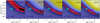 |
Fig. 23 EPF analysis of the first three 13CO transitions observed from an MHD clump. Results are shown for five Tkin values around the reference value Tref. The images show the χ2 planes for noiseless observations but assuming 20% error estimates. The contours are drawn at χ2 = 1 (blue contour) and χ2 = 2 (cyan contour). The minimum χ2 values (average over the three transitions) are quoted in the frames. The white dots correspond to the χ2 minima for 50 noise realisations consistent with the 20% observational noise. |
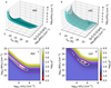 |
Fig. 24 Examples of χ2 distributions in PEP and LOC analysis CS and C34S spectra of a BE model with M = 2 M⊙ and Tkin = 15 K. The upper frames show the general shape of the χ2 = 24 surfaces. The lower frames show cross-sections at the correct temperature of Tkin = 15 K. The white contours are drawn at χ2 = 7, 16, 32 and the magenta contours at χ2 = 64 and 128, where the χ2 values are the direct average over the included transitions (J = 1–0, 2–1, and 3–2 for CS and C34S). |
6 Conclusions
We present PEP, a new computer programme for the parallel calculation of line intensities based on the escape probability formalism (EPF). The comparison to other programmes and the analysis of synthetic observations of spherically symmetric model clouds and clumps extracted from a MHD simulation have led to the following conclusions.
The PEP programme is found to be robust, with results that are in good agreement with predictions from other EPF programs.
The parallelisation and the batch mode of calculating many parameter combinations in a single run make the calculations efficient. In our tests, the calculations with 100 × 100 density and column density values took about one second.
In the tested cases, single-precision floating point arithmetic provided sufficient accuracy. This can lead to some speed gains in GPU calculations.
The full coverage of parameter grids provides useful information on the uncertainties and especially on the parameter degeneracies. However, the other major source of uncertainty are model errors, which can be probed only by examining full RT calculations of alternative models.
For synthetic observations of spherical cloud models, the EPF predictions were often inconsistent with the expected density and column density values. The discrepancy can be more than a factor of 2, even without any observational errors.
The kinetic temperature is often poorly constrained and even a small error in Tkin can be associated with a large shift (up to a factor of a few) in the predicted n(H2) and column density values. This is especially true when the lines are close to saturation due to high optical depths.
The analysis of MHD clumps showed the EPF estimates to be usually correct to within a factor of 2 (models with variable abundances and correct Tkin values). Different molecules showed varying amounts of systematic errors. There were a few outliers with errors of an order of magnitude and not limited to just optically very thick lines.
The overall shape of the χ2 surfaces can be similar in EPF and full RT calculations. However, in the particular case when a the RT model approximates the source structure well, the full RT calculations will provide more accurate parameter estimates. RT modelling is also needed in studies of the line profiles or whenever deviations from the source’s homogeneity are clear.
In this paper, we discuss the approximate handling of hyperfine structure lines in EPF calculations. The results were qualitatively similar to those seen in full non-local RT calculations. However, EPF is clearly not suitable in some cases, for example, for modelling hyperfine anomalies.
Overall, the model errors can be as important or even more important than the observational errors and should be taken into account when estimating the overall reliability of the EPF analysis. The accuracy of parameter estimates could also be improved if some of the parameters had fixed values or tight priors. These could be based on ancillary observations, such as direct Tkin measurements with other species or even rough N(H2) estimates from independent dust observations.
Acknowledgements
M.J. acknowledges the support of the Research Council of Finland Grant No. 348342.
Appendix A Hyperfine structure lines
In the normal EPF method, the photon escape probabilities are calculated for isolated Gaussian line profiles. However, many molecules exhibit hyperfine structure (HFS), where the interaction of molecular rotation with an atomic nucleus of non-zero spin results in the splitting of the energy levels. Typical astro-nomical observations of HFS spectra include the low rotational transitions of N2H+, HCN, HNC, and C17O, as well as the inversion transitions of ammonia, especially NH3 (1,1) and NH3(2,2). When spectral lines are split to a number of components along the frequency axis, the individual HFS components have lower optical depths, and this results in an overall increase in the photon escape probability β. Since β is a non-linear function of τ, it scales differently for HFS components of different intensity, even before the additional complication of potential frequency overlap between HFS components is taken into account. The spectral overlap depends on the assumed velocity field and the line width FWHM. HFS is therefore not a simple rescaling of the normal β values and must be estimated separately for each species and values of the optical depth and line FWHM.
The normal EPF criteria may not be meaningful in the case of HFS lines. Under the LVG assumption the emission from every hyperfine component could be absorbed by any other hyperfine component. In real clouds this is possible only between neighbouring components, typically over a frequency interval corresponding to some ~1 km s−1 in velocity.
We tested one possible method to take into account the HFS effects, under the assumption that the relative level populations of the HFS components are in LTE. The β values are first calculated in the normal fashion for Gaussian lines (i.e. according to either the LVG, slab, or homogeneous-sphere model). For the HFS transitions these are rescaled with correction factors ξ(τ) = β(HFS)/β(Gaussian). Here β (Gaussian) is the normal escape probability for isolated Gaussian line profiles. To calculate ξ, we assume a static medium with the prescribed line FWHM, and compute the correction ξ(τ) for a single line of sight, as a function of the total optical depth.
The escape probability for a Gaussian line in a static medium is
![Mathematical equation: $\[\beta(\text {Gaussian})=\frac{\int \phi(\nu) e^{-\tau \phi(\nu)} d \nu}{\int \phi(\nu) d \nu},\]$](/articles/aa/full_html/2025/04/aa53409-24/aa53409-24-eq7.png) (A.1)
(A.1)
where ϕν is the profile function with ∫ ϕνdν = 1. For NC HFS components with velocity offsets Δvi, the corresponding expression for an HFS line is
![Mathematical equation: $\[\beta(\mathrm{HFS})=\frac{\int \sum_i^{N_{\mathrm{C}}} I_i \phi\left(\nu+\Delta \nu_i\right) e^{-\tau_\nu^{\Sigma}} d \nu}{\int \sum_i^{N_{\mathrm{C}}} I_i \phi\left(\nu+\Delta \nu_i\right)} .\]$](/articles/aa/full_html/2025/04/aa53409-24/aa53409-24-eq8.png) (A.2)
(A.2)
The optical depth τΣ is the sum over the components,
![Mathematical equation: $\[\tau_\nu^{\Sigma}=\tau \sum_i^{N_{\mathrm{C}}} I_i \phi\left(\nu+\Delta \nu_i\right),\]$](/articles/aa/full_html/2025/04/aa53409-24/aa53409-24-eq9.png) (A.3)
(A.3)
where τ is the total line optical depth. Here Ii are the relative weights of the HFS components with ∑iIi = 1. Thus the denominator of Eq. (A.2) is again equal to one.
In the absence of specific information on the source velocity field, the proposed method is only one possible way to estimate the actual β values in a source. However, it captures the expected increase for β of the HFS transition and is an improvement over simply ignoring the HFS structure.
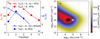 |
Fig. A.1 Comparison of EPF results for N2H+ when the HFS of the J = 1 − 0 line is taken into account (Sect. A) or is ignored. Frame a shows the Tex and TR values for Tkin = 20 K, with n(H2) = 105 cm−3 and N(N2H+) = 1014 cm−2 (cyan circle in frame b). The assumed line width is FWHM = 1 km s−1. Frame b shows the ratio of Tex(1-0) values when the HFS is taken into account and when it is ignored. |
Figure A.1 compares PEP calculations where the hyperfine structure of the J = 1 − 0 line of N2H+ is either ignored or taken into account. The inclusion of the hyperfine structure naturally increases the photon escape probability and leads to significant decrease in the excitation temperature of the J = 1 − 0 transition. The difference is reflected in the J = 2 − 1 transition, while the next levels remain practically unchanged. Figure A.1b shows the ratio of the predicted Tex(1 − 0) values over a wide range of n(H2) and N(H2). The effect has a maximum of close to a factor of 2, but it disappears at high densities due to thermalisation.
For comparison with the above approximation, we performed one calculations with LOC, using a homogeneous spherical model with a temperature of Tkin=20 K. While PEP provides a single set of level populations and thus a single value of Tex, in LOC results the excitation varies radially. Therefore the results of the two programs are not expected to be identical even without the HFS structure. To characterise the LOC models we used the mean column density over the projected model area and the mean value of Tex over the model volume.
Figures A.1 and A.2 show that the effect of the hyperfine structure, and the location and general shape of the parameter region where the inclusion of hyperfine structure causes a large drop in Tex are similar. However, the Tex(HFS)/Tex(no – HFS) minimum is in PEP calculations at a higher density and lower column density.
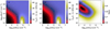 |
Fig. A.2 Results from LOC runs with homogeneous spherical models and the N2H+ molecule. Frames a and b show, respectively, the mean Tex(1 − 0) values when the J = 1 − 0 hyperfine structure is ignored or is taken into account. Frame c shows their ratio and is analogous to the PEP results in Fig. A.1. The axes are the mean values of the model cloud density n(H2) and N2H+ column density. The gas kinetic temperature is Tkin = 20 K. |
Appendix B PEP run times
To characterise the PEP performance in terms of run times, we ran a series of tests using the CO molecule, with Tkin = 15 K and including the first 20 rotational levels. PEP was run for different sizes of the (n, N) grid, which however always covered the same total range of parameter values. The iterations were stopped when the change in level populations per iteration was less than 10−5 in relative terms or less than 10−10 in absolute terms. The latter ensures that levels with insignificant population do not prevent the iterations from stopping.
The run times are shown in Fig. B.1a. For most practical applications (i.e. with up to a few times 104 parameter combinations per run), the run time is roughly constant and less than one second. Thus, the cost is dominated by the initialisations done in the host Python programme. Thereafter the run times approach the expected linear dependence on the number of parameter combinations. In the test system, GPU becomes faster than CPU only when the number of parameter combinations is above a few times 104. The GPU results in Fig. B.1 are shown for a modern laptop, using an external desktop GPU. Unexpectedly, there was no significant difference in calculations performed in single precision and double precision. Because the main computational cost in the solving of the statistical equilibrium equations and that scales with the third power of the number of excitation levels, the advantage of using GPUs (and single precision) should become significant in larger problems, although this was not yet observed in our tests.
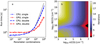 |
Fig. B.1 Examples of PEP run times. Frame a shows the run time on CPU (blue curve) and GPU (red curve) as a function of the number of parameter combinations (n, N) for Tkin=15 K. The calculations included the first 20 rotational levels of the CO molecule. The black dashed line indicates the slope of a one-to-one relation. Frame b shows how the number of iterations needed to reach the selected convergence criteria. |
Figure B.1b shows the parameter ranges and the number of iterations required by the PEP programme. As noted in Sect. 2, the initial level populations are set in according to the LTE condition with T = Tkin. This also partially explains the low number of iterations needed at the highest densities, where the solution remains close to LTE. However, at high column densities and somewhat lower volume densities (optically thick but non-thermalised lines), it might be necessary to check further that the iterations have not ended prematurely, due to a slower convergence.
Appendix C Additional Bonnor-Ebert models
C.1 Model spectra for Bonnor-Ebert spheres
Figures C.1-C.5 show synthetic spectra for BE models that were used as inputs in the EPF analysis in Sect. 4.1. Each plot shows the spectra for three values of the model Tkin and mass, each frame including line profiles for the first five rotational transitions observed with the FWHM = R0/3 beam. Optically less thick species (C18O, C34S, and H13CO+) are not plotted as these have always nearly Gaussian profiles.
Figure C.6 shows the EPF analysis of an isothermal Bonnor-Ebert model separately for three 12CO and 13CO transitions. The figure is thus similar to Fig. 5 except for the use of different molecules and the more massive model cloud of M = 10 M⊙.
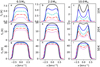 |
Fig. C.1 Synthetic 12CO spectra for 1D BE models. |
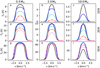 |
Fig. C.2 Synthetic 13CO spectra for 1D BE models. |
C.2 Plots for isothermal Bonnor-Ebert models
Section 4.1.1 discussed the results for isothermal BE spheres. Figure 7 showed the discrepancy between the reference values and the EPF estimates for one of the cloud models. Figures C.7-C.10 show further examples for four models of different mass and temperature Tkin.
Figure C.11 shows χ2 planes for 13CO observations of the isothermal BE sphere with M =2 M⊙ and Tkin=20 K, for analysis performed at three different Tkin values. The figure is similar to Fig. 8 but for a model where results are more sensitive to the assumed value of Tkin.
Figure 12 showed EPF-predicted χ2 values for one BE cloud model, for combined CS and C34S observations, with the C34S abundances that were either correct or had an error of 50%. Figure C.12 shows additional examples for the 2 M⊙ cloud models with two values of Tkin.
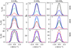 |
Fig. C.3 Synthetic 13CO spectra for 1D BE models. |
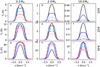 |
Fig. C.4 Synthetic CS spectra for 1D BE models. |
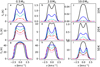 |
Fig. C.5 Synthetic HCO+spectra for 1D BE models. |
C.3 Non-isothermal Bonnor-Ebert models
Figures C.13 and C.14 show a comparison of EPF results for non-isothermal models and the combination of CS and C34S lines. The kinetic temperature is fixed to the correct value, but the analysis is also repeated with C34S abundances that are 50% lower or higher than the actual value. The figures differ only by the radial Tkin gradient being positive in Fig. C.13 and negative in Fig. C.14.
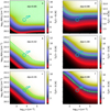 |
Fig. C.6 Same as Fig. 5 but for 12CO (left frames) and 13CO (right frames), for the cloud model with 10M⊙ and Tkin=20 K. |
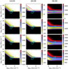 |
Fig. C.11 Same as Fig. 8, but for 13CO spectra of the isothermal BE model with M = 2M⊙ and Tkin=20 K. |
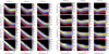 |
Fig. C.12 Same as Fig. 12, but for the 2M⊙ cloud model with Tkin=10 K (left frames) and Tkin=20 K (right frames). |
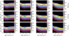 |
Fig. C.13 Results for BE models with M = 0.5 M⊙ and ⟨Tkin⟩=10 K, for Tkin increasing outwards. The frames from left to right correspond to the combination of 1-4 lowest rotation transitions of CS and C34S. The rows correspond to three assumptions of the C34S abundance (middle row with the correct value). Contours are drawn at χ2=1, 2, 10, and 100 (red, cyan, magenta, and blue colours, respectively). The cyan circles indicate the reference values for the central line of sight (smallest circle), for the FWHM = R0/3 beam (as used for the input synthetic observations), and for the FWHM = R0 beam (largest circle). |
Appendix D Additional figures on MHD clumps
Section 4.2 showed results for clumps selected from the MHD simulation. The discrepancy between the reference values and EPF estimates based on 12CO and 13CO observations were shown in Figs. 20-21. Figures D.1-D.9 show further examples for other molecules and models with (ad hoc) higher density.
References
- Asensio Ramos, A., & Elitzur, M. 2018, A&A, 616, A131 [NASA ADS] [CrossRef] [EDP Sciences] [Google Scholar]
- Bernes, C. 1979, A&A, 73, 67 [NASA ADS] [Google Scholar]
- Bonnor, W. B. 1956, MNRAS, 116, 351 [NASA ADS] [CrossRef] [Google Scholar]
- Bron, E., Daudon, C., Pety, J., et al. 2018, A&A, 610, A12 [CrossRef] [EDP Sciences] [PubMed] [Google Scholar]
- Cannon, C. J. 1973, ApJ, 185, 621 [Google Scholar]
- Commerçon, B., Hennebelle, P., Audit, E., Chabrier, G., & Teyssier, R. 2010, A&A, 510, L3 [NASA ADS] [CrossRef] [EDP Sciences] [Google Scholar]
- de Jong, T., Chu, S., & Dalgarno, A. 1975, ApJ, 199, 69 [NASA ADS] [CrossRef] [Google Scholar]
- Dullemond, C. P., & Turolla, R. 2000, A&A, 360, 1187 [NASA ADS] [Google Scholar]
- Ebert, R. 1955, Z. Astrophys., 37, 217 [NASA ADS] [Google Scholar]
- Goldreich, P., & Scoville, N. 1976, ApJ, 205, 144 [NASA ADS] [CrossRef] [Google Scholar]
- Goldsmith, P. F. 2001, ApJ, 557, 736 [Google Scholar]
- Gonzalez-Alfonso, E., & Cernicharo, J. 1993, A&A, 279, 506 [NASA ADS] [Google Scholar]
- Harries, T. J., Haworth, T. J., Acreman, D., Ali, A., & Douglas, T. 2019, Astron. Comp., 27, 63 [NASA ADS] [CrossRef] [Google Scholar]
- Hogerheijde, M. R., & van der Tak, F. F. S. 2000, A&A, 362, 697 [NASA ADS] [Google Scholar]
- Holdship, J., Viti, S., Martín, S., et al. 2021, A&A, 654, A55 [NASA ADS] [CrossRef] [EDP Sciences] [Google Scholar]
- Juvela, M. 1997, A&A, 322, 943 [NASA ADS] [Google Scholar]
- Juvela, M. 2020, A&A, 644, A151 [NASA ADS] [CrossRef] [EDP Sciences] [Google Scholar]
- Juvela, M., & Ysard, N. 2011, ApJ, 739, 63 [NASA ADS] [CrossRef] [Google Scholar]
- Juvela, M., Padoan, P., & Jimenez, R. 2003, ApJ, 591, 258 [NASA ADS] [CrossRef] [Google Scholar]
- Juvela, M., Mannfors, E., Liu, T., & Tóth, L. V. 2022, A&A, 666, A74 [NASA ADS] [CrossRef] [EDP Sciences] [Google Scholar]
- Navarro-Almaida, D., Le Gal, R., Fuente, A., et al. 2020, A&A, 637, A39 [NASA ADS] [CrossRef] [EDP Sciences] [Google Scholar]
- Neufeld, D. A., & Kaufman, M. J. 1993, ApJ, 418, 263 [NASA ADS] [CrossRef] [Google Scholar]
- Neufeld, D. A., Lepp, S., & Melnick, G. J. 1995, ApJS, 100, 132 [Google Scholar]
- Padoan, P., Juvela, M., Pan, L., Haugbølle, T., & Nordlund, Å. 2016, ApJ, 826, 140 [NASA ADS] [CrossRef] [Google Scholar]
- Peters, T., Banerjee, R., Klessen, R. S., & Mac Low, M.-M. 2011, ApJ, 729, 72 [Google Scholar]
- Roueff, A., Pety, J., Gerin, M., et al. 2024, A&A, 686, A255 [NASA ADS] [CrossRef] [EDP Sciences] [Google Scholar]
- Rybicki, G. B., & Hummer, D. G. 1992, A&A, 262, 209 [NASA ADS] [Google Scholar]
- Schöier, F. L., van der Tak, F. F. S., van Dishoeck, E. F., & Black, J. H. 2005, A&A, 432, 369 [Google Scholar]
- Shirley, Y. L. 2015, PASP, 127, 299 [Google Scholar]
- Sobolev, V. V. 1960, Moving Envelopes of Stars (Cambridge: Harvard University Press) [Google Scholar]
- Tomida, K., Tomisaka, K., Matsumoto, T., et al. 2013, ApJ, 763, 6 [NASA ADS] [CrossRef] [Google Scholar]
- Tunnard, R., & Greve, T. R. 2016, ApJ, 819, 161 [NASA ADS] [CrossRef] [Google Scholar]
- Tunnard, R., Greve, T. R., Garcia-Burillo, S., et al. 2015, ApJ, 815, 114 [NASA ADS] [CrossRef] [Google Scholar]
- van der Tak, F. F. S., Black, J. H., Schöier, F. L., Jansen, D. J., & van Dishoeck, E. F. 2007, A&A, 468, 627 [NASA ADS] [CrossRef] [EDP Sciences] [Google Scholar]
- van Zadelhoff, G. J., Dullemond, C. P., van der Tak, F. F. S., et al. 2002, A&A, 395, 373 [NASA ADS] [CrossRef] [EDP Sciences] [Google Scholar]
All Figures
|
Fig. 1 PEP and RADEX results for density n(H2) = 103 cm−3, column density of the species N = 1015 cm−2, and a 1 km s−1 linewidth. The temperature is Tkin = 20 K for the CO (left frames), Tkin = 10 K for the HCO+(middle frames), and Tkin = 100 K for the H2O (right frames) runs. The plots show the fractional upper level population nu, excitation temperature Tex, optical depth τ, and the radiation temperature TR for the first seven transitions. PEP results are shown for single-precision (PEP) and double-precision (PEP-D) runs and for a pure Python implementation without parallelisation (“PEP-Py”). |
| In the text | |
|
Fig. 2 CO level populations for Tkin = 70 K, n(H2) = 104 cm−3, N(CO) = 1018 cm−2, and FWHM = 1 km s−1. The upper frame shows the level populations for all 22 levels (J = 0–21), and the lower frame shows the level populations relative to the double-precision PEP calculations. |
| In the text | |
|
Fig. 3 Example of optically thick CO emission from a 10 M⊙ BE model with Tkin = 10 K. Frame a shows spectra, frame b Tex profiles, and frame c the radial variation in the photon escape probability β. Results are shown for full non-LTE calculations with LOC (solid lines), for constant excitation equal to the mean values of the LOC solution (“⟨LOC⟩”, dashed lines), and for the LTE case at Tkin (dotted lines). Frames a–b show data for the first three transitions (black, blue, and red, respectively) but, for clarity, frame c includes only the J = 1–0 and J = 3–2 transitions. |
| In the text | |
|
Fig. 4 PEP results for 13CO spectra towards a BE sphere with Tkin = 10 K and M = 2 M⊙. The colour scale shows the predicted line intensities as a function of volume and column density. In the green hatched areas PEP predictions are within 10% of the observed line intensities. The circles indicate the reference cloud parameters for the central LOS (small circle), along with the beam average with FWHM = R0/3 (middle circle corresponding to the beam in the synthetic observations) and for FWHM = R0 (large circle). |
| In the text | |
|
Fig. 5 PEP analysis of CS (left frames) and C34S (right) line intensities. The plotted symbols are as in the previous figures. The cloud model is the same as in the previous figures, with M = 2 M⊙ and Tkin = 20 K. Each frame quotes the depth of the possible self-absorption dip as the line intensity at the line centre divided by the maximum intensity. |
| In the text | |
|
Fig. 6 Combined χ2 values in PEP analysis of 13CO spectra. The cloud model an isothermal BE sphere with M = 10 M⊙ and Tkin = 20 K. The frames a-d correspond, respectively, to the combinations of the 1–4 first rotational transitions. The circles indicate the reference values towards its centre (smallest circle), averaged over a FWHM = R0/3 beam (middle circle that corresponds to the synthetic observations), and averaged over a FWHM = R0 beam (largest circle). |
| In the text | |
|
Fig. 7 Results for seven molecules observed towards an isothermal BE sphere with M = 0.5 M⊙ and Tkin = 20 K. Frame a shows the minimum χ2 value (blue open circles) and χ2 value for the reference density and column density (red filled circles). Frames b and c, respectively, show the ratio of density and column density values at the χ2 minimum relative to the reference values. Each molecule is plotted with four markers that, from left to right, correspond to the combination of the lowest transitions (1–4). |
| In the text | |
|
Fig. 8 Plots of χ2 in the EPF analysis of 13CO lines. The analysis used three Tkin temperatures, as listed above each column of frames. The cloud model is an isothermal BE sphere with M = 10 M⊙ and Tkin = 20 K. First row shows the analysis of the J = 1 − 0 lines, and each subsequent row adds one further rotational transition. The contours are drawn at χ2 levels of 1 (red), 2 (cyan), 10 (magenta), and 100 (blue contour). In order of increasing size, the circles indicate the reference density and column density values towards the model centre, averaged over a FWHM = R0/3 beam (used for the synthetic observations), and averaged over a FWHM = R0 beam. |
| In the text | |
|
Fig. 9 Change in the minimum-χ2 PEP solution for 13CO spectra as a function of Tkin. The model is a 10 M⊙ BE sphere with Tkin = 20 K. Frame a shows the minimum value of χ2 (solid lines) and the χ2 value for the reference parameter values (dashed lines). Frame b shows the predicted density and frame c the predicted column density. The cyan, magenta, and red colours correspond, respectively, to the analysis using two, three, or four transitions. |
| In the text | |
|
Fig. 10 Same as Fig. 9, but for the synthetic 13CO observations of the M = 2 M⊙ and Tkin = 20 K model. |
| In the text | |
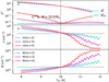 |
Fig. 11 Same as Fig. 9, but for C34S observations of the M = 10 M⊙, Tkin = 10 K model. |
| In the text | |
|
Fig. 12 Estimated χ2 for combined CS and C34S observations of a BE sphere with M = 0.5 M⊙ and Tkin = 10 K. The columns correspond to the assumed C34S abundances (correct and with ±50% errors). The first row shows results for the J = 1 − 0 line, and each subsequent row adds one more rotational transition. |
| In the text | |
|
Fig. 13 Results for 13CO spectra of the M = 2 M⊙ BE model with ⟨Tkin⟩ = 10 K. The case is similar to that of Fig. 4, except that Tkin increases outwards. |
| In the text | |
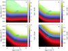 |
Fig. 14 Same as Fig. 13, but with Tkin decreasing outwards. |
| In the text | |
|
Fig. 15 Values of χ2 as function of density and column density for a non-isothermal 2M⊙ model with ⟨Tkin⟩ = 10 K and Tkin increasing outwards. Frame a is based on the fit to 12CO J = 1–0 spectra, and each subsequent frame includes to the analysis one further rotational level. |
| In the text | |
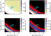 |
Fig. 16 Same as Fig. 15, but with Tkin decreasing outwards in the model cloud. |
| In the text | |
|
Fig. 17 Example of a clump extracted from the MHD model. The frames show the 13CO(2-1) line-area maps at the full resolution (frame a) and for observations with FWHM = 0.31 pc (frame b) and FWHM = 0.61 pc (frame c) beam sizes. The fractional abundance is spatially constant. |
| In the text | |
|
Fig. 18 PEP results for a MHD clump, using the Tkin value given in frame a. Each frame shows χ2 for one molecule and its first three rotational transitions. The cyan circles indicate the beam-averaged model mean densities and column densities (sizes in order of increasing FWHM). The χ2 values are based on the medium beam size. The blue, cyan, magenta, and red contours correspond to χ2 = 1, 2, 10, and 100. |
| In the text | |
|
Fig. 19 Same as Fig. 18 but for a model with density-dependent abundances. The reference values are shown without (cyan circles) and with the weighting by fractional abundances (magenta circles). The circle sizes correspond to the three beam sizes, in order of increasing FWHM. The χ2 values correspond to observations with the intermediate beam size. |
| In the text | |
|
Fig. 20 Comparison of EPF estimates and reference values for 12CO spectra observed with the intermediate beam size. Frames a and b correspond, respectively, to the constant and variable abundance cases. The marker colours show the χ2 ratio between the rref and rest positions. In frame b, the red text refers to one outlier with ratios greater than 10. |
| In the text | |
|
Fig. 21 Same as Fig. 20 but for the 13CO observations. Blue text in frame b refers to one outlier with both ratios below 0.05. |
| In the text | |
|
Fig. 22 Same as Fig. 21, but using estimates from the global χ2 minimum instead of the closest position rest along the χ2 valley. |
| In the text | |
|
Fig. 23 EPF analysis of the first three 13CO transitions observed from an MHD clump. Results are shown for five Tkin values around the reference value Tref. The images show the χ2 planes for noiseless observations but assuming 20% error estimates. The contours are drawn at χ2 = 1 (blue contour) and χ2 = 2 (cyan contour). The minimum χ2 values (average over the three transitions) are quoted in the frames. The white dots correspond to the χ2 minima for 50 noise realisations consistent with the 20% observational noise. |
| In the text | |
|
Fig. 24 Examples of χ2 distributions in PEP and LOC analysis CS and C34S spectra of a BE model with M = 2 M⊙ and Tkin = 15 K. The upper frames show the general shape of the χ2 = 24 surfaces. The lower frames show cross-sections at the correct temperature of Tkin = 15 K. The white contours are drawn at χ2 = 7, 16, 32 and the magenta contours at χ2 = 64 and 128, where the χ2 values are the direct average over the included transitions (J = 1–0, 2–1, and 3–2 for CS and C34S). |
| In the text | |
|
Fig. A.1 Comparison of EPF results for N2H+ when the HFS of the J = 1 − 0 line is taken into account (Sect. A) or is ignored. Frame a shows the Tex and TR values for Tkin = 20 K, with n(H2) = 105 cm−3 and N(N2H+) = 1014 cm−2 (cyan circle in frame b). The assumed line width is FWHM = 1 km s−1. Frame b shows the ratio of Tex(1-0) values when the HFS is taken into account and when it is ignored. |
| In the text | |
|
Fig. A.2 Results from LOC runs with homogeneous spherical models and the N2H+ molecule. Frames a and b show, respectively, the mean Tex(1 − 0) values when the J = 1 − 0 hyperfine structure is ignored or is taken into account. Frame c shows their ratio and is analogous to the PEP results in Fig. A.1. The axes are the mean values of the model cloud density n(H2) and N2H+ column density. The gas kinetic temperature is Tkin = 20 K. |
| In the text | |
|
Fig. B.1 Examples of PEP run times. Frame a shows the run time on CPU (blue curve) and GPU (red curve) as a function of the number of parameter combinations (n, N) for Tkin=15 K. The calculations included the first 20 rotational levels of the CO molecule. The black dashed line indicates the slope of a one-to-one relation. Frame b shows how the number of iterations needed to reach the selected convergence criteria. |
| In the text | |
|
Fig. C.1 Synthetic 12CO spectra for 1D BE models. |
| In the text | |
|
Fig. C.2 Synthetic 13CO spectra for 1D BE models. |
| In the text | |
|
Fig. C.3 Synthetic 13CO spectra for 1D BE models. |
| In the text | |
|
Fig. C.4 Synthetic CS spectra for 1D BE models. |
| In the text | |
|
Fig. C.5 Synthetic HCO+spectra for 1D BE models. |
| In the text | |
|
Fig. C.6 Same as Fig. 5 but for 12CO (left frames) and 13CO (right frames), for the cloud model with 10M⊙ and Tkin=20 K. |
| In the text | |
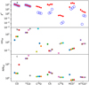 |
Fig. C.7 Same as Fig. 7, but for the M = 0.5M⊙ model with Tkin=10 K |
| In the text | |
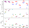 |
Fig. C.8 Same as Fig. 7, but for the M = 0.5M⊙ model with Tkin=50 K |
| In the text | |
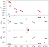 |
Fig. C.9 Same as Fig. 7, but for the M = 10M⊙ model with Tkin=10 K |
| In the text | |
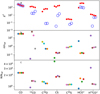 |
Fig. C.10 Same as Fig. 7, but for the M = 10M⊙ model with Tkin=50 K |
| In the text | |
|
Fig. C.11 Same as Fig. 8, but for 13CO spectra of the isothermal BE model with M = 2M⊙ and Tkin=20 K. |
| In the text | |
|
Fig. C.12 Same as Fig. 12, but for the 2M⊙ cloud model with Tkin=10 K (left frames) and Tkin=20 K (right frames). |
| In the text | |
|
Fig. C.13 Results for BE models with M = 0.5 M⊙ and ⟨Tkin⟩=10 K, for Tkin increasing outwards. The frames from left to right correspond to the combination of 1-4 lowest rotation transitions of CS and C34S. The rows correspond to three assumptions of the C34S abundance (middle row with the correct value). Contours are drawn at χ2=1, 2, 10, and 100 (red, cyan, magenta, and blue colours, respectively). The cyan circles indicate the reference values for the central line of sight (smallest circle), for the FWHM = R0/3 beam (as used for the input synthetic observations), and for the FWHM = R0 beam (largest circle). |
| In the text | |
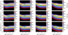 |
Fig. C.14 Same as Fig. C.13, but with Tkin decreasing outwards in the model cloud. |
| In the text | |
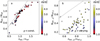 |
Fig. D.1 Same as Fig. 20, but for models with five times higher volume density. |
| In the text | |
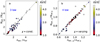 |
Fig. D.2 Same as Fig. 20, but for the HCO+molecule. |
| In the text | |
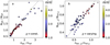 |
Fig. D.3 HCO+results similar to Fig. D.2, but for models with five times higher volume density. |
| In the text | |
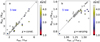 |
Fig. D.4 Same as Fig. 20, but for the H13CO+molecule. |
| In the text | |
 |
Fig. D.5 H13CO+results. Same as Fig. D.4, but for models with five times higher density. |
| In the text | |
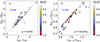 |
Fig. D.6 Same as Fig. 20, but for the CS molecule. |
| In the text | |
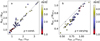 |
Fig. D.7 CS results similar to Fig. D.6, but for models with five times higher volume density. |
| In the text | |
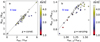 |
Fig. D.8 Same as Fig. 20, but for the C34S molecule. |
| In the text | |
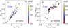 |
Fig. D.9 C34S results similar to Fig. D.8, but for models with five times higher volume density. |
| In the text | |
Current usage metrics show cumulative count of Article Views (full-text article views including HTML views, PDF and ePub downloads, according to the available data) and Abstracts Views on Vision4Press platform.
Data correspond to usage on the plateform after 2015. The current usage metrics is available 48-96 hours after online publication and is updated daily on week days.
Initial download of the metrics may take a while.