| Issue |
A&A
Volume 696, April 2025
|
|
|---|---|---|
| Article Number | A163 | |
| Number of page(s) | 19 | |
| Section | Interstellar and circumstellar matter | |
| DOI | https://doi.org/10.1051/0004-6361/202452974 | |
| Published online | 25 April 2025 | |
From filament to clumps and cores
A multiscale study of fragmentation and the role of the magnetic field and gas velocity in the infrared dark cloud SDC18.624-0.070
1
Academia Sinica, Institute of Astronomy and Astrophysics, No. 1, Sec. 4, Roosevelt Rd., Taipei, Taiwan
2
Department of Physics, National Taiwan University, No. 1, Sec. 4, Roosevelt Rd., Taipei, Taiwan
3
Jodrell Bank Centre for Astrophysics, Department of Physics and Astronomy, The University of Manchester, Manchester M13 9PL, UK
4
I. Physikalisches Institut, Universität zu Köln, Zülpicher Str. 77, 50937 Köln, Germany
5
Intituto de Astrofísica de Andalucía (CSIC), Glorieta de la Astronomía s/n, 18008 Granada, Spain
6
Cardiff Hub for Astrophysics Research & Technology, School of Physics & Astronomy, Cardiff University, Queens Buildings, The parade, Cardiff CF24 3AA, UK
★ Corresponding author.
Received:
13
November
2024
Accepted:
24
February
2025
Abstract
Aims. Fragmentation is a multiscale process forming structures with sizes that vary by several orders of magnitude. However, multiscale investigations of the magnetic field characterizing its properties across the physical scales relevant to the fragmentation process (filaments and clouds, clumps, and cores) are elusive. In this work, we present a multiscale study of the magnetic field using polarization continuum observations with various resolutions.
Methods. We made use of data from the JCMT and the SMA at 850 μm and 1.3 millimeter (mm) wavelengths to study the filamentary infrared dark cloud SDC18.624-0.070. Our observations cover filament (~ 10 pc), filament-embedded clump (~ 1 pc), isolated clump (~ 0.1 pc), and clump-embedded core (~ 0.01) scales, which are key to investigating the impact of the magnetic field on fragmentation.
Results. We found a magnetic field that is predominantly perpendicular to the major axes of all structures (filament, clumps, and cores). While its circular mean orientations are preserved within about 20°, a systematically increasing field dispersion toward smaller scales indicates the growing impact of gravity. Velocity gradients traced by N2H+, with a resolution similar to that of the polarization observations, also tend to be perpendicular to the filament’s major axis. All these features suggest that the magnetic field constrains the direction of accretion and initial contraction, as predicted by strong-field models.
Conclusions. We argue that the observed magnetic field and velocity gradient can result from a combination of converging flows, based on a detected SiO component along the filament, and rotation, based on the measured N2H+ specific angular momentum profile. A multiscale energy analysis of gravity, magnetic field, and turbulence quantifying their relative importance shows that SDC18-S, despite displaying less fragmentation, has a larger field strength than SDC18-N, which harbors more fragments. A faster (SDC18-N) and slower evolution (SDC18-S) to a gravity-dominated regime has been found to explain the different fragmentation at clump-embedded core scale, with the stronger magnetic field in SDC18-S suppressing fragmentation to a greater extent.
Key words: ISM: clouds / ISM: magnetic fields / ISM: individual objects: SDC18.624-0.070
© The Authors 2025
 Open Access article, published by EDP Sciences, under the terms of the Creative Commons Attribution License (https://creativecommons.org/licenses/by/4.0), which permits unrestricted use, distribution, and reproduction in any medium, provided the original work is properly cited.
This article is published in open access under the Subscribe to Open model. This email address is being protected from spambots. You need JavaScript enabled to view it. to support open access publication.
1 Introduction
Interstellar filaments play an important role in star formation. Herschel observations have demonstrated that molecular clouds are highly filamentary and most of the star-forming clumps and cores form within filaments through fragmentation (e.g., André et al. 2014; Hacar et al. 2023). Understanding how fragmentation occurs is crucial, especially for the case of high-mass star formation. This is because massive stars are believed to form prevailingly in a clustered environment where significant fragmentation is expected to take place (McKee & Ostriker 2007; Rathborne et al. 2015; Pineda et al. 2023). Theoretical models predict the properties of fragments, for instance, the number, mass, size, and distribution are determined by the interplay of physical mechanisms such as gravity, magnetic field, and turbulence (e.g., Commerçon et al. 2011; Howard et al. 2016; Federrath et al. 2017). Observationally, the role of the magnetic field in star formation is still elusive compared to other mechanisms. A linear polarization of the dust continuum is often used to trace magnetic field orientations, rotated by 90 degrees, assuming the alignment of the minor axis of dust grains with the magnetic field (e.g., Hildebrand et al. 1984; Lazarian & Hoang 2007). However, while the fragmentation is a multiscale process forming structures with sizes differing by several orders of magnitude, multiscale investigations of the magnetic field, characterizing its properties across the physical scales relevant to the fragmentation process (clouds, clumps, and cores) remain limited (e.g., Li et al. 2015; Ching et al. 2017; Tang et al. 2019; Pattle et al. 2023).
Within the various phases of the interstellar medium (ISM), infrared dark clouds (IRDCs) are dense molecular clouds that were first detected as high-extinction dark features against the bright Galactic near- and mid-infrared background. They are cold (T < 25K), very massive (M ~ 103 - 105 M⊙), and very dense (nH2 ≥ 103 cm−3). They are also considered to be the sites of massive star formation at an early evolutionary stage (Peretto & Fuller 2010; Ragan et al. 2011). SDC18.624-0.070 (hereafter SDC18) is a filamentary IRDC at a distance of 3.7 kpc (Sridharan et al. 2002) with a north–south elongation around 10 pc that has been extensively studied with multiwavelength data (Sridharan et al. 2002; Beuther et al. 2002, 2010, 2015; Beuther & Steinacker 2007; Fallscheer et al. 2009; Peretto & Fuller 2009; Tackenberg et al. 2014, also see Figure 1). The Planck polarization data display a uniform large-scale magnetic field perpendicular to the major axis of the filament (Figure 1, Planck Collaboration Int. XLII 2016). Using N2H+ (1–0) line data from the Plateau de Bure Interferometer (PdBI), Beuther et al. (2015) found a velocity gradient perpendicular to the major axis of the filament. SDC18 harbors objects at various evolutionary stages from starless to protostellar clumps (Beuther et al. 2010), where the two most evolved ones, SDC18-N and SDC18-S, have garnered significant interest. SDC18-N (or IRAS18223-1243) is a highmass protostellar object (HMPO) that is detected up to the IRAC 3.5 μm band (Sridharan et al. 2002). It is reported to be the host of an ultra-compact HII region and have HCO+ (1–0) infall signatures (Kavak et al. 2021; Liu et al. 2020). SDC18-S (or IRDC18223-3) is likely to be a less evolved object that is bright at 24 μm and known to drive an outflow but shows no emission in the IRAC bands (Beuther & Steinacker 2007; Fallscheer et al. 2009). All the other sources are quiescent and have weak or no emission at 24 μm. These diverse properties of clumps in SDC18 provide a good testing bed for studying the effect of the magnetic field on high-mass star formation.
In this work, we present a multiscale magnetic field study of SDC18 using dust polarization continuum observations with three different resolutions from the James Clerk Maxwell Telescope (JCMT) and the Submillimeter Array (SMA). Our observations cover filament (∼10 pc), filament-embedded clump (~ 1 pc), isolated clump (~ 0.1 pc), and clump-embedded core (~ 0.01 pc) scales, which are key to investigating and understanding the fragmentation processes in this star-forming region. These results, combined with the gas kinematics from N2H+ observations with similar resolutions, reveal the evolution of the relative importance of gravity, magnetic field, and turbulence over scale, along with its impact on the structure formation toward smaller scales. Altogether, this offers insights into the possible formation mechanism of the SDC18 filament. The paper is organized as follows. In Section 2, we describe the observations and data reduction. Section 3 presents the results of our polarization observations and their connection with the N2H+ line observations. Section 4 discusses fragmentation and possible trends together with gravity, magnetic, and turbulent energies, as well as their implications for the formation mechanism of SDC18. Finally, our conclusions are given in Section 5.
2 Observations and data reduction
2.1 JCMT/POL-2
Continuum polarization observations toward SDC18 were carried out using the POL-2 polarimeter on the Submillimeter Common User Bolometer Array 2 (SCUBA-2) of the JCMT 15 m telescope in July 2017. The continuum polarization observations were conducted at 450 and 850 μm wavelengths simultaneously, but this work focuses on the 850 μm data, which have an angular resolution of 14.6ʺ. We adopted the POL-2 DAISY scan mode, which covered two fully sampled circular fields of 11ʹ centered on (α, δ) = (18h25m10.62s, – 12°42ʹ44ʹʹ.2) and (18h25m08.33s, – 12°45ʹ23ʹʹ.2). All the data were taken in band 1 weather with a 225 GHz opacity τ225 < 0.05. The total integration time was 4.6 hr.
The POL-2 data were reduced with the pol2map command in the Starlink package1 following the standard procedure. The detailed algorithms of the SCUBA-2 reduction process are described in Chapin et al. (2013). The skyloop algorithm was invoked to reduce uncertainties due to combining multiple observations simultaneously. The POL-2 data reduction was done with a 4′′ pixel size, but the output Stokes I, Q, and U maps were binned to a pixel size of 7′′ to improve the sensitivity while preserving the Nyquist sampling. A POL-2 flux conversion factor (FCF) of 725 Jy beam−1 pW−1 at 850 μm was used for the three Stokes I, Q, and U parameters (Friberg et al. 2016). This resulted in noise levels of 4.2 mJy beam−1 for Stokes Q and U and 6.4 mJy beam−1 for Stokes I near the center of the map. The uncertainty increases away from the center of the field and becomes a factor of ~2 higher at the edge. The debiased polarization intensity PI, its uncertainty σPI, the polarization fraction P, and its uncertainty σP were derived using the equations:
 (1)
(1)
 (2)
(2)
 (3)
(3)
 (4)
(4)
where σI, σQ, and σU are the uncertainties of the Stokes I, Q, and U parameters. The polarization angle θ and its uncertainty σθ were calculated as
 (5)
(5)
and
 (6)
(6)
2.2 SMA
The SMA polarization observations towards SDC18-N and SDC18-S were carried out in subcompact, compact, and extended array configurations at 1.3 mm between June 2021 and July 2022. In total, five tracks were executed. The phase reference centers were at (α, δ) = (18h25m10.61s, – 12°42ʹ25ʹʹ.0) for SDC18-N and (α, δ) = (18h25m08.49s, – 12°45ʹ22ʹʹ.0) for SDC18-S. The details of the observations are listed in Table 1. The full polarization mode of the SMA Wideband Astronomical ROACH2 Machine (SWARM) receiver was used (Primiani et al. 2016). The SWARM receiver has a bandwidth of 12 GHz per sideband with a fixed channel width of 140 kHz separated by an intermediate frequency (IF) of 4–8 GHz. The frequency ranges covered were 209.3–221.3 GHz and 229.3–241.3 GHz for the lower and upper sidebands. Both continuum and line data such as 13CO (2–1) and C18O (2–1) were obtained. This work focuses on the continuum. Instrumental polarization calibration, self-calibration for Stokes I, and imaging were performed in the MIRIAD package (Sault et al. 1995). The model derived from the self-calibration of the Stokes I component was then applied to the calibration of the Stokes Q and U components. The Stokes I, Q, and U data were independently deconvolved using the MIRIAD task CLEAN. The polarized intensity, polarization position angle, and polarization fraction along with their uncertainties were derived from the Stokes I, Q, and U maps using the MIRIAD task IMPOL. The resulting flux density calibration is accurate to within 10%, based on a comparison between the measured flux densities of quasars in each track with the reported fluxes in the SMA observatory database.
To probe the magnetic field at different spatial scales, two data sets with different resolutions were generated from different combinations of tracks. The data with baselines shorter than 50kλ in all five tracks were used, along with a Gaussian taper of a 2.2ʺ full-width-half-maximum (FWHM) to produce lowerresolution maps with a synthesized beam of 4.41ʺ × 3.32ʺ. The largest recovered angular scale θLAS is 52.2ʺ, which is estimated by  , where λ is the observing wavelength and Bmin is the length of the shortest baseline. This results in an root mean square (rms) noise of 0.79 mJy beam−1 for Stokes I and 0.21 mJy beam−1 for Stokes Q and U maps. We note that the cut of 50kλ is a compromise between sensitivity and beam size, optimized to image the clump-scale magnetic field in this source. All the data in the compact and three extended tracks, where the uv-baseline coverage is between 9.9 to 163.3 kλ, were combined to produce higher-resolution maps with a synthesized beam of 1.45ʺ × 1.25ʺ. The θLAS here is 25.6ʺ. This leads to a difference in resolution by a factor of about 8 in area, which allows us to distinguish among the larger clumps and the smaller cores to probe fragmentation. The rms noise levels in the higher-resolution maps are 0.38 mJy beam−1 for Stokes I and 0.19 mJy beam−1 for Stokes Q and U.
Summary of SMA observations.
2.3 Molecular line data
We additionally observed the J = 2–1 transition of silicon monoxide (SiO) toward SDC18 using the IRAM-30m telescope. This observation was motivated as a probe of possible converging flows (see Section 4.1.1). The observations were performed in September 2022 using the on-the-fly (OTF) mapping mode toward the center (α, δ) = (18h25h10.00h, – 12°44ʹ00ʹʹ.0) with a map size of 7.2ʹ × 2.4ʹ and a beam size of 30ʺ. The EMIR receiver was used along with the VESPA spectrometer to provide a spectral resolution of 20 kHz (0.07 km s−1). The data were reduced with the standard procedure using the CLASS package of the GILDAS software and binned to a velocity resolution of 0.28 km s−1 to improve the sensitivity. The typical rms noise was 0.03 K ( ) per 0.28 km s−1 channel.
The gas kinematics in SDC18 from filament to clumps and cores were traced by observations with N2H+, a dense gas tracer (Bergin & Tafalla 2007), at three different resolutions similar to those of the dust continuum polarization. Using the same gas tracer helps minimize the systematic uncertainty when observing gas with different physical properties with different molecular species. The pc-scale gas dynamics of the filament is seen in N2H+ (1–0) with the IRAM-30m with a resolution of 27ʺ (Peretto et al. 2015). The sub-pc scale gas is mapped in N2H+ (1–0) with the PdBI with a resolution of 5.77ʺ × 3.39ʺ, where the uv-baselines range from 4.6 to 53.7 kλ (Beuther et al. 2015). N2H+ (3–2) is used in SDC18-S to probe a 0.01 pc scale with the SMA with a resolution of 2.28ʺ × 1.11ʺ with uv-baselines ranging from 11 to 189 kλ (Fallscheer et al. 2009). There are currently no N2H+ observations with a similarly high resolution available for SDC18-N. The structures covered in continuum using the SMA and in gas probed with N2H+ are similar in the available data. All the interferometric data suffer from missing the flux at scale larger than 52ʺ and 26ʺ for clumps and cores, respectively. However, the sizes of the dense clumps and cores are about 20ʺ and 15ʺ, respectively. The impact of recovery of the largest angular scales of the interferometric data on our results is negligible.
3 Results
In this section, we present the observational results obtained from the JCMT and SMA observations. We refer to the 10 pc scale as the entire SDC18 filament with the length of about 10 pc, the 1 pc scale as filament-embedded clumps identified by the dendrogram with sizes of about 1 pc in the JCMT data, the 0.1 pc scale as isolated clumps seen in the lower-resolution SMA data with sizes around 0.1 pc where the extended structures are filtered out, and the 0.01 pc scale as clump-embedded cores seen in the higher-resolution SMA data revealing fragments with sizes around 0.01 pc within larger clumps. More details on the properties of polarized emission for both the JCMT and SMA observations are given in Appendix A.
3.1 JCMT dust continuum and polarized emission – Filament and filament-embedded clumps
The JCMT/POL-2 850 μm continuum emission (Stokes I component) of SDC18 is presented in panel (a) of Figure 2. This total intensity map clearly depicts the 10 pc long filament along the north–south direction as well as the two filament-embedded clumps, SDC18-N and SDC18-S (marked as orange contours in Figure 1) residing in its northern and southern parts with a separation of ∼3ʹ (∼3.2 pc). We estimated the orientation of SDC18 by eye to be about 12° from north to east, taking advantage of its simple filamentary geometry. To determine the boundaries of SDC18-N and SDC18-S in the JCMT map for a comparison with clump properties at smaller scale seen in the higher-resolution SMA maps (Section 3.2), we performed a dendrogram analysis (Rosolowsky et al. 2008) on the JCMT total intensity map using the Python package astrodendro. We set a lower limit of 3σI and a minimum area of one JCMT beam (14.6ʺ) for the dendrogram to identify structures. The minimum difference for structures to be separated as independent entity is also set to be 3σI. The resulting boundaries of SDC18-N and SDC18-S are shown in orange contours in Figure 1, which roughly enclose the same regions as the 500 mJy beam−1 contours.
The segments in panel (a) of Figure 2 show the plane-ofsky (POS) magnetic (B-)field orientations, inferred from a 90° rotation of the polarization orientations in SDC18. The median uncertainties of polarization orientations detected with a S/N of 2σP and 3σP are 9.1° and 7.2°, respectively. Overall, the Bfield is perpendicular to the major axis of the filament (~ 12°), with an estimated circular mean position angle of 115° over the entire filament. Panel (a) of Figure 3 shows the circular mean and dispersion of field position angles for different regions along the filament, averaged within boxes of 100ʺ × 100ʺ along the filament ridge. Most of the regions have mean field orientations similar to the overall mean of 115° except for the northernmost area. The magnetic field is rather ordered within the filament- embedded clumps, with a circular mean and angular dispersion of 96±16° for SDC18-N and 131±11°for SDC18-S (Table C.1).
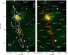 |
Fig. 1 Spitzer images of SDC18 at 24 μm (red), 8 μm (green), and 5.8 μm (blue), together with JCMT/POL-2 850μm dust continuum contours (left panel) and magnetic field structures (right panel). The contours denote the 50, 500, and 1000 mJy beam−1 of the JCMT total intensity. Orange contours are the boundaries of SDC18-N and SDC18-S at filament-embedded clump scale determined by the dendrogram analysis. The JCMT/POL-2 magnetic field orientations with P> 3σP are in yellow and in red for 3σP > P > 2σP. White segments are the larger-scale Planck magnetic field orientations inferred from 90° rotation of polarization at 353 GHz (∼ 5ʹ) in a pixel size of 103ʺ. |
3.2 SMA dust continuum and polarized emission – Isolated clumps and clump-embedded cores
Panel (b) and (c) of Figure 2 show the 1.3 mm dust continuum emission of SDC18-N and SDC18-S from the SMA with a resolution of ~4ʺ overlapped with the POS magnetic field orientations selected with I > 15σI and P > 2σP. The uncertainties of the magnetic field position angles with a S/N of 2σP and 3σP are 7.2° and 6.4°, respectively. At this resolution, both clumps are single-peaked, but extended (except for the small secondary peak located south-west of the main peak in SDC18-S), while the larger-scale emission is filtered out. This allows us to study the clumps isolated from the larger-scale filamentary surrounding. We derived a position angle of 169° for SDC18-N and 21° for SDC18-S by fitting an ellipse to their boundaries defined by a 15σI flux level (see Section 4.2). The magnetic field at this isolated clump scale has a circular mean orientation and angular dispersion of 93±37° for SDC18-N and 130 19° for SDC18-S (Figure 3 (b), Figure 3 (c); see Table C.1). Both orientations are nearly perpendicular to the elongation of the clumps and fairly well aligned with the larger scale magnetic field seen in the JCMT/POL-2 data. This suggests that the B-field preserves its mean orientation during the fragmentation from a filament to a clump scale (see also Figure 9). However, the magnetic field in individual sub-regions of the clumps shows more distinct patterns that are different from the overall mean orientation. This is reflected by larger angular dispersion values, namely, 37° and 19°, as compared to 16° and 11° in the larger scale JCMT data. Pinched magnetic field structures, possibly tracing an hourglass- like magnetic field geometry, are found in the northern and southern parts of SDC18-N, as well as on the western side of SDC18-S. Significant depolarization is found in the eastern part of SDC18-S. These features may be further linked to the fragmentation and magnetic field structures at even smaller scale, as described in the following.
The higher resolution (~ 1.3ʺ) SMA dust continuum observations at 1.3mm for SDC18-N and SDC18-S are shown in panels (d) and (e) of Figure 2 together with magnetic field orientations for I > 7σI and P > 2σP. The uncertainties of the B-field position angles are 11.0° for 2σP and 7.6° for 3σP detection. We note that we have applied different total intensity thresholds when selecting polarization detections from observations of three different resolutions due to their different sensitivities and dynamic ranges. While this is not yet resolved in the 4ʺ SMA maps, SDC18-N now appears further fragmented once observed at higher resolution; namely, multiple and clearly spatially separated cores form along the major axis of the clump (Figure 2, panel (d)). On the other hand, SDC18-S shows no further fragmentation with emission mostly concentrated on its main peak (Figure 2, panel (e)). At this higher resolution, we can observe the cores as they are embedded in the larger clumps. The magnetic field shows circular mean orientations and angular dispersion values of 97±38° and 135±38° for all cores together in SDC18-N and SDC18-S, respectively. This continues the trend seen from the filament-embedded clump to isolated-clump scales where the magnetic field has retained a similar overall mean orientation, while displaying an increasingly larger dispersion toward smaller scale.
Individual cores on the SMA higher-resolution (1.3ʺ) maps are identified and shown in panel (d) and (e) of Figure 3. Cores in SDC18-N were identified using the dendrogram analysis with a lower limit of 7σI, a minimum area of one beam (1.3ʺ), and a minimum difference for structures to be separated as independent entity of 3σI. For SDC18-S where no further fragmentation is seen, we took the 7σI contours as the boundaries of the main and secondary core. We calculated the position angles of the major axes of the individual cores by fitting ellipses on the core boundaries, in the same way as we did at the larger scale. The mean magnetic field within each individual core is estimated, except for core 2 in SDC18-N (Figure 3(d)) where no polarization is detected. The major axes and the mean magnetic field orientations of the individual cores are plotted in Figure 3(d) and Figure 3(e), demonstrating that the magnetic field orientations are close to perpendicular to the individual cores’ major axes. The only exception is the southernmost core in SDC18-N (core 4 in Figure 3(d)), where the core’s major axis is rather aligned with its mean magnetic field orientation with an angle of about 20°. In the following sections, our analysis at clump-embedded core scale is focused on the cores with significant polarization detections (N–1, N–3, and S–1).
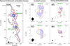 |
Fig. 2 (a): SDC18 continuum emission at 850 μm with an angular resolution of 14.6ʺ with JCMT/POL-2 in contours and magnetic field segments, capturing the entire filament and the filament-embedded clumps, SDC18-N and SDC18-S (green boxes), zoomed in the middle and right panels. The contours are 50, 500, and 1000 mJy beam−1. (b), (c): Continuum emission at 1.3 mm in contours and magnetic field segments of SDC18-N (b) and SDC18-S (c) with an angular resolution of 4.41ʺ × 3.32ʺ with the SMA, capturing the isolated clumps resolving out diffuser and more extended emission. Solid black contours represent the Stokes I flux levels at 15, 40, and 80σI, while dashed black contours show -5σI. (d), (e): The same as the middle panels but with an angular resolution of 1.45ʺ × 1.25ʺ, capturing the clump-embedded cores revealing fragmentation of the larger clump. Solid black contours are 7, 30, and 45σI Stokes I flux levels, while dashed black contours are -7σI. The segments in all panels show magnetic field orientations with P > 3σP detections in blue and 3σP > P > 2σP detections in red. The right panels display magnetic field segments gridded at half of the synthesized beam resolution. The segments in the middle panels are overgridded for a sharper visualization, but only data at half of the synthesized beam are used for the further analysis. |
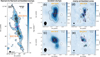 |
Fig. 3 Circular mean magnetic field orientations in different regions and scales of SDC18. The black segments in panel (a) show the magnetic field orientations averaged within boxes of 100ʺ × 100ʺ along the filament ridge, overplotted on the JCMT continuum map. The intersection angles of the grey segments are the dispersion values of the field orientations. The locations of the segments are the average locations of the detected polarization signals within each box. The purple segment and intersection angle of the violet segments show the overall circular mean of 115° with its dispersion of 45° of the magnetic field orientations within the entire filament. The red and green segments in all panels present the mean magnetic field orientations and position angles of the major axes for the clumps and cores at different scales. Magenta contours mark the boundaries of the individual cores in the SMA 1.3ʺ resolution maps for SDC18-N (panel (d)) and SDC18-S (panel (e)) identified in Section 3.2. |
3.3 Gas kinematics across multiple scales
Figure 4 shows the centroid velocity and velocity dispersion maps of N2H+ at multiple scales. The molecular line parameters are derived from hyperfine line fittings on the N2H+ data cubes using the Python package PySpecKit (Ginsburg & Mirocha 2011). The hyperfine line transitions of N2H+ are modelled by the built-in routine “n2hp_vtau” which fits multiple Gaussians to the spectra. The IRAM-30m observation traces the whole filament region such as the JCMT dust continuum observation, while the PdBI observation is centered on the spine of the filament. Both centroid velocity maps (Figure 4 panel (a) and (c)) reveal a velocity gradient across the filament in east-west orientation. In the southern part of the filament, where the gas is red-shifted to the east and blue-shifted to the west, the velocity gradient from the IRAM-30m data is ~2 km s−1 pc−1. However, toward the northern section of the filament above Dec = – 12°43ʹ00ʹʹ.0, the velocity gradient appears to be reversed in direction with the eastern side blue-shifted and the western side red-shifted with a smaller magnitude of ~0.8 km s−1 pc−1. This flip in the direction of gas motion can possibly be a signpost of ongoing star-formation activities of evolved high-mass protostellar objects in SDC18-N, where either the outflow or the expanding HII region can affect the large-scale gas dynamics (Beuther et al. 2015). On the other hand, velocity gradients with opposite directions, perpendicular to a filament’s axis, can also be a signpost of filament formation by turbulent converging flows. In this scenario, the inhomogenous nature of the accreting material means that its angular momentum is not constant along the length of the filament. Thus, different regions in the filament may locally rotate in directions independent of each other, leading to a flipping of radial velocity gradient directions. This has been seen both in simulated (Clarke et al. 2018) and observed filaments formed by converging flows (e.g., Schneider et al. 2010). More details of the converging flow scenario are discussed in Section 4.1.1.
From the SMA N2H+ (3–2) data, Fallscheer et al. (2009) reported a velocity gradient along a northeast-southwest direction, which is perpendicular to the reported outflow axis with a position angle of 135°. This is suggestive of core rotation. We discuss this case further in Section 4.1.2.
At the filament scale, the magnetic field and velocity gradient are both prevailingly perpendicular to the filament’s major axis and aligned with each other. To illustrate this alignment, we compute the absolute differences in position angles between the magnetic field and velocity gradient by rebinning the JCMT 14ʹʹ.6 polarization data to match the lower-resolution (27ʺ) IRAM-30m N2H+ velocity data. In the left panel of Figure 5, we show the histogram of these local differences (from every location with a matched magnetic field–velocity gradient pair). With a circular mean of 20°, this prevailing overall alignment between magnetic field and velocity gradient is suggestive of a scenario where either the gas motion toward the filament is guided by the magnetic field or, alternatively, the strong gas flow is entraining the magnetic field. To test which mechanism is more dominant, we calculated the energetics of the magnetic field and gas motion quantified by the magnetic pressure, PB, and ram pressure, Pram = ρV, at the filament scale. We took the gas velocity as V = 0.75 km s−1, which is the velocity difference from the ridge to the edge of the filament, from the IRAM 30m N2H+ map. Estimates of the other parameters are given in Section 4.2. We find PB = 8.13 10−9 dyn cm−2 and Pram = 2.41 10−10 dyn cm−2. The higher magnetic pressure suggests that the gas motion is likely to be controlled by the magnetic field. This is consistent with an interpretation of a dynamically important magnetic field model (see Sections 4.1 and 4.3 for more discussion).
To further investigate the spatial distribution of the magnetic field-velocity gradient alignment, we also present a map of this alignment in the right panel of Figure 5. We find that larger angle differences tend to reside on the outskirt of the filament. This is a feature that is also seen in, for example, the G34.43 filamentary cloud which also displays perpendicular magnetic field and velocity gradients (Tang et al. 2019). This might be a sign indicating that the alignment is further enhanced by gravity when the gravitational pull becomes stronger toward the higher-density regions and clumps of the filament.
On a smaller scale, the outflow and rotation axis of SDC18S (panel (e) in Figure 4) is along the clump-scale mean magnetic field (panel (c) in Figure 3). This might suggest efficient magnetic braking and could be a factor suppressing fragmentation because a significant amount of angular momentum will be transferred out of the central part of the clump. In return, this can then facilitate the accretion of material onto a single object (Hennebelle et al. 2011). Indeed, in the presented higher resolution SMA data, SDC18-S does not seem to fragment further. We defer a deeper interpretation of the gas kinematics to Section 4.
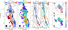 |
Fig. 4 SDC18 N2H+ centroid velocity and dispersion maps at various scales. Panels (a) and (b) show the IRAM-30m N2H+ (1–0) centroid velocity and velocity dispersion map with a resolution of 27ʺ. The black dashed line in the first panel marks Dec = – 12°43ʹ00ʹʹ.0 where the direction of the velocity gradient flips. Panels (c) and (d) are the N2H+ (1–0) centroid velocity and velocity dispersion map with a beam size of 5.77ʺ × 3.39ʺ from the PdBI. Panels (e) and (f) are the N2H+ (3–2) centroid velocity and velocity dispersion map of SDC18-S observed by the SMA with a beam size of 2.28ʺ × 1.11ʺ. The same black contours representing JCMT total intensity levels at 50, 500, and 1000 mJy beam−1, identical to the left panel of Figure 2, are shown in the first four panels. The SMA total intensity contours of 7, 30, and 45σ (identical to the lower right panel of Figure 2) are shown in the two maps on the very right. In panel (e), a black dot and arrow mark the continuum peak and the outflow orientation in SDC18-S reported by Fallscheer et al. (2009). |
3.4 Extended SiO emission along the 10 pc filament
We present SiO (2–1) observations to investigate the spatial distribution of SiO along the SDC18 filament. The implication of the presence of SiO will be discussed in Section 4.1.1. The integrated intensity (moment 0) map of SiO is shown in Figure 6 along with representative spectra extracted from selected positions. The SiO emission consists of two components. A spatially extended but spectrally narrower component is detected toward the central and the northern part of the filament, with typical FWHM line widths of 3–5 km s−1 obtained from single-Gaussian fits (upper and middle right panels in Figure 6). Additionally, a spatially compact component with a broader linewidth larger than 10 km s−1 has been found to coexist with the narrower-linewidth component in the area of SDC18-S. An example of such a spectrum where the linewidths of the broader and narrower components are measured by a twocomponent Gaussian fit is shown in the bottom right panel in Figure 6.
4 Analyses and discussion
4.1 Filament formation mechanism and dynamics
At the filament scale, the POL-2 polarization data show that the mean magnetic field is prevailingly perpendicular to the major axis of SDC18. Moreover, the N2H+ line observations also suggest a velocity gradient perpendicular to the filament major axis, as reported by Beuther et al. (2015). Hence, a prevailing alignment between local magnetic field orientations and local velocity gradients is found (Section 3.3). In this section, we discuss the possible interpretation of these observed characteristics of SDC18. It is worth noting that the perpendicular velocity gradient may arise from multiple mechanisms related to the filament formation process. In short, combining all the observational evidence, we will suggest that the SDC18 filament can be formed in a post-shock layer compressed by large-scale converging flows with a non-zero impact parameter.
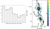 |
Fig. 5 Histogram (left panel) and map (right panel) of absolute differences in position angles between magnetic field orientations and velocity gradients. The black contours are the same JCMT total intensity levels at 50, 500, and 1000 mJy beam−1, as in the left panel of Figure 2. |
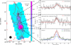 |
Fig. 6 Left: SDC18 SiO (2–1) integrated intensity map from the IRAM-30m. The 3σ intensity level is marked by the black contour. Red contours show the same JCMT total intensity levels of 50, 500, and 1000 mJy/beam as in panel (a) in Figure 2. Right: Spectra extracted from several positions marked by the black dashed lines. In the upper two panels, the red lines are the single-Gaussian fits, while in the bottom panel, the red line is the combination of a two-component Gaussian fit including a broader and narrower component in green and blue, respectively. |
4.1.1 Observational evidences of converging flow models
Large-scale turbulent converging flows generating dense postshock regions are suggested to be one of the major channels responsible for the formation of filaments (Pineda et al. 2023). In the post-shock layer, anisotropic accretion proceeding preferentially along the magnetic field lines leads to magnetic field orientations and velocity gradients perpendicular to a filament’s major axis, as shown in the Serpens South region in Chen et al. (2020). In this scenario, continuous accretion of matter from the converging flows induces low-velocity shocks. This can leave chemical fossil records of shock tracers, such as SiO, which can then be released from dust grains (Schilke et al. 1997). Due to the extended nature and low velocity (<10 km s−1) of the colliding flows, SiO emission in regions formed by converging flows will be widespread (>1 pc2) and have relatively narrow (≲3–6 km s−1) line widths. This extended SiO emission due to colliding flows is seen both in simulations (Louvet et al. 2016) and observational surveys of IRDCs (e.g., Jiménez-Serra et al. 2010; Cosentino et al. 2018, 2020; Armijos-Abendaño et al. 2020; Kim et al. 2023).
In contrast to the scenario of converging flows, the SiO emission produced by outflows can span size scales from sub-pc to about 1 pc and is associated with young stellar objects (e.g., Gibb et al. 2007; Sánchez-Monge et al. 2013; Liu et al. 2021). Outflows have velocities ranging from 10 to 100 km s−1 or higher, so the SiO emission associated with outflows can also have a larger line width.
Given these characteristics, the spatially extended SiO emission in SDC18 of a few pc with relatively narrow linewidths, not clearly associated with young stellar objects, is likely pointing at the existence of colliding flows. The spatially compact and spectrally broader component detected toward SDC18-S is likely to arise from the outflow of a source reported by Fallscheer et al. (2009).
Turbulence driven by the accretion flow converts a fraction of the kinetic energy of the accreted material into turbulent energy (Clarke et al. 2017). The mass accretion rate, therefore, can be estimated from the observed property of the shocked gas traced by the SiO line and serve as a probe of whether the converging flow scenario is valid. Heitsch (2013) shows that the velocity dispersion σacc driven by accretion can be calculated as
 (7)
(7)
where ϵ is the efficiency of accretion energy converting into turbulent energy, Rf is the filament radius, vacc is the inflow velocity of the accreting gas, Mline is the filament mass per unit length, and Ṁline is the filament mass accretion rate. We adopt an efficiency ϵ = 0.1, as proposed by Clarke et al. (2017). The velocity dispersion σacc driven by accretion is measured from the widespread SiO component to be 3 km s s−1 (Section 3.4). The mass per unit length of SDC18 is estimated to be ~313 M⊙ pc−1 by dividing the filament mass by the filament length of 10 pc and the filament radius is estimated to be 0.23 pc. The detailed derivation of these parameters is presented in Section 4.2 and listed in Table C.1. Assuming a typical inflow velocity of 5–10 km s−1 that can release SiO from dust grains (Louvet et al. 2016), we obtain a mass accretion rate of 140–580 M⊙ pc−1 Myr−1, which is similar to the values found in other accreting massive IRDCs (e.g., Williams et al. 2018; Chen et al. 2019). This indicates that SDC18 can accrete its current mass in 0.5–2 Myr, which is in the range of the typical filament formation timescale (Pineda et al. 2023). In conclusion, combining the properties of the magnetic field, gas dynamics, and the estimated formation timescale of the filament, our observational results support a scenario where the SDC18 IRDC can be formed through converging flows.
4.1.2 Rotation signature and converging flows with non-zero impact parameter
Aside from accretion flows, the observed velocity gradients perpendicular to the major axis of SDC18 could also be reminiscent of rotation. An observational feature of rotating objects is the dependence of their specific angular momentum on radius ( j(r) ∝ ra). This dependence can vary as the size of the rotating structures changes (Belloche 2013). For clouds, clumps, and cores with scales larger than ~0.01 pc, the specific angular momentum is found to decrease with radius with a power-law index a ~ 1.4–1.6 (Goldsmith & Arquilla 1985; Goodman et al. 1993; Tatematsu et al. 2016).
In order to investigate how the specific angular momentum, j, evolves across different scales in SDC182, we measure it as a function of radius, j(r) = r × Vrot, from the N2H+ data at different resolutions. Vrot = |V(r) - Vc| is the rotational velocity calculated as the difference between the velocity at radius r, V(r), and the velocity at the center, Vc, assuming the velocity gradients trace rotation. The radial angular momentum profile is averaged along the ridge defined in Section 4.2 for the IRAM-30m and PdBI data. For the SMA data the rotational velocity is calculated in northeast-southwest direction and averaged along the outflow axis. In Figure 7, we show the radial specific angular momentum profile in log-log scale, where the bin sizes are taken to be one- third of the beams for each data set. A linear fit on the profile for a combination of all data sets gives a power-law index a of 1.35 ± 0.10 ( j(r) r1.35±0.10), which is consistent with the angular momentum relation of rotating cloud samples from previous studies (e.g., Goldsmith & Arquilla 1985). On the other hand, the best-fit a from a combination of the SMA and PdBI data (sampling the smaller scales at r<0.19 pc) and from the IRAM-30m data only (sampling the larger scales at r≥0.19 pc) is 1.64 and 1.91, respectively.
We emphasize that the above analysis of the specific angular momentum assumes that the velocity gradients exclusively trace rotation. In reality, the velocity gradients likely originate from a combination of rotation (likely dominating at smaller scales) and from accretion flows (likely dominating at larger scales). Indeed, we observe differences in their respective power-law indices when fitting only for larger or smaller scales. In particular, we find a tentative deviation in the power-law index of the specific angular momentum as a function of radius (a ~ 1.9) from the typical range (a = 1.4–1.6) when fitting the large-scale gas dynamics from the IRAM-30m data only. The presence of a (different) rotational velocity component on such a large scale is a natural consequence of converging flows in a non-head-on collision scenario (Balfour et al. 2017). Moreover, such collisions may be statistically more common than the idealized head-on collision in the general simulations of converging flows. In such a scenario, the prestructures collide with a non-zero impact parameter which generates angular momentum via shear motions. This initial angular momentum can then be enhanced later on during the contraction of material and formation of filaments by conservation of angular momentum and render the formed filament in rotation. Such a scenario has indeed been proposed for the IRDC SDC13, where Wang et al. (2022) found a relatively uniform pc-scale magnetic field (from the JCMT), except for an arc-like “U-shaped” feature along the western boundary of the central hub. The larger 10-pc scale magnetic field (from Planck) was found to display a partial spiral-like converging pattern, which is locally aligned with the small-scale field in the northeastern side, but is perpendicular to the U-shape field in the western side. Along with an analysis of the gas dynamics, Wang et al. (2022) argued that the variation of the large- and small-scale field geometry is caused by the collision of large-scale flows with non-zero impact parameters which distorts the magnetic field (see Figure 15 of Wang et al. (2022)). If this is also the case for SDC18, we note that the system should be viewed more edge-on to the collision (i.e., the LOS that is perpendicular to the collision axis) to produce the perpendicular magnetic field in projection. Future studies of this scenario, including MHD simulations with a similar setup, are needed to further investigate the 3D magnetic field and gas dynamics structures with their observational features.
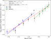 |
Fig. 7 Radial profile of specific angular momentum for SDC18 from N2H+ observations covering different scales. |
4.2 Magnetic field strength-density scaling: From embedded to isolated and fragmenting clumps
In this section, we investigate the physical properties of the entire SDC18 filament, as well as SDC18-N and SDC18-S at the scales we defined; namely, filament (~ 10 pc), filament-embedded clump (~ 1 pc), isolated clump (~ 0.1 pc), and clump-embedded core (~ 0.01 pc) scales, using the data sets with different resolutions described in the previous sections. The resulting physical parameters are summarized in Table C.1. The main goal in this section is then to use these parameters across the different scales to investigate the scaling relation between the density, n, and magnetic field strength, B.
The effective radius (Reff) of the filament can be estimated to be 0.23 pc from averaging fitted 1D Gaussians on the crosssection cuts along the filament ridge. A constant position angle of 12° is assumed for the ridge and cuts are perpendicular to the ridge in every pixel, where the ridge is taken from the continuum peak of SDC18-S toward the upper and lower parts of the entire filament. For the filament-embedded clump (∼1 pc) scale, the effe✓ctive radii of SDC18-N and SDC18-S are calculated as  . Here, a and b are the lengths of the semi-major and semi-minor axes of the elliptical fits of the clump boundaries defined by the dendrogram algorithm applied on the JCMT total intensity map. At smaller scales, the boundaries are defined as the 15σI flux level on the lower resolution (4ʺ) SMA maps for the isolated clump (~ 0.1 pc) scale and as the 7σI flux level on the higher resolution (1.3ʺ) SMA maps for the clump-embedded core (~ 0.01 pc) scale.
For the filament and filament-embedded clump scale, we adopted temperatures (T ) from the dust temperature maps derived from Hi-GAL data using the PPMAP algorithm (Marsh et al. 2017), where the average temperatures are 20 K for the entire SDC18 filament, 22 K for SDC18-N, and 18 K for SDC18-S. The uncertainty on T for these two scales is estimated from the standard deviation of the dust temperature maps. For the isolated clump and clump-embedded core scales, we adopted T=36 K, which is derived from a combination of LTE modeling of several molecular lines (CH3CCH, H2CS and CH3CN) and dust SED modeling for SDC18-S (Lin et al. 2022). As there is no uncertainty of T given at these scales, we assume an uncertainty of 10%, similar to the values obtained for the larger scales. The column density, NH2 , was converted from the JCMT total intensity map, Iν, for the filament and filament-embedded clump scales, and from the SMA total intensity maps, Iν, for isolated clump and clump-embedded core scales as
 (8)
(8)
where Bν(T ) is the Planck function at a temperature, T , while κν = 0.1(ν/1THz)2 cm2/g is the dust opacity per unit mass (Beckwith et al. 1990), μ = 2.8 is the mean molecular weight per hydrogen molecule, and mH is the mass of a hydrogen atom. We adopted an uncertainty of 36% on κν, which comes from a 23% uncertainty of the gas-to-dust ratio and a 28% uncertainty of the dust opacity derived by Sanhueza et al. (2017).
The resulting total masses, M, are derived by integrating the column density within the boundaries of the structures at each scale as defined above. The uncertainty of M is propagated from the errors of the measured intensity, temperature and dust opacity. For the SDC18 filament as a whole, the H2 number density, nH2 , is calculated from the column density divided by the filament width (= 2Reff), which is assuming a line-of-sight (LOS) dimension for the filament equivalent to its POS extension in an east-west direction. For all the smaller scales for SDC18- N and SDC18-S,  , which assumes oblate structures.
The velocity dispersion σv of filament and clumps are averaged within their respective boundaries from the N2H+ velocity dispersion maps at the different resolutions (Section 3.3). For SDC18-N at the clump-embedded core scale where no equivalent high-resolution N2H+ observations are available, NH3 (1,1) line data from VLA with a resolution of ~3ʺ (Lu et al. 2014) are used instead. Previous studies demonstrate that the two molecular species often show similar linewidths (e.g., Hacar et al. 2017), though they have very different critical densities. The nonthermal velocity dispersion (σv,NT) is then calculated as  where k is the Boltzmann constant and m is the mass of either the N2H+ or NH3 molecule. The FWHM of the lines is then derived as
  . As presented in Section 3.3, SDC18 displays a velocity gradient over multiple scales across the filament and clumps. Such kinematics could cause additional line broadening other than thermal and turbulent broadening and affect the calculation of related physical parameters. To remove this effect from the estimated line widths, we assume: (1) the velocity gradient is linear; (2) the intensity distribution of the filament and clumps is uniform; (3) the magnitude of the velocity gradient is the same for both the POS and LOS directions. The above assumptions lead to a uniform distribution in velocity in both the POS and LOS directions. Then, the square of the broadening due to the velocity gradient will be given by the variance of the uniform distribution (e.g., Clapham et al. 2014),
  , where (Vmax −Vmin) is the velocity difference across the density structure due to the velocity gradient. For each scale, the velocity difference is estimated from the velocity gradient obtained from N2H+ maps with different resolutions multiplied by their (linear) beam sizes in the POS, or by the diameters (2Reff) of the structures in LOS directions. The corrected nonthermal velocity dispersion (
 ) is then calculated as
  . We note that the assumption of uniform intensity distribution leads to an upper limit of the estimated broadening, given that the more realistic centrally peaked intensity distribution has a smaller variance. Overall, the broadening from velocity gradients accounts for ~20% of the nonthermal velocity dispersion at most. Hence, the inclusion or exclusion of this effect will not change the results of our analysis or the relative importance of gravity, magnetic field, and turbulence (see Section 4.4).
With all of this taken into consideration, the POS magnetic field strength (Bpos), when adopting the Davis– Chandrasekhar–Fermi (DCF, Davis 1951; Chandrasekhar & Fermi 1953) method, can be derived for every scale as:
 (9)
(9)
where ρ = μmHnH2 is the gas volume density, δϕ is the magnetic field angular dispersion, and Q is a factor accounting for the magnetic field entanglement along the LOS and within the telescope beam, which we assume to be Q = 0.5 (Ostriker et al. 2001). The DCF method assumes that the field angular dispersion solely results from turbulence. While this may be correct at the filament and filament-embedded clump scales, we resolved clear hourglass-like shapes at the isolated clump and clump-embedded core scales (Section 3), which likely arise from gravitational collapse.
In order to isolate the dispersion of a turbulent magnetic field component from other larger-scale distortions, such as gravity, we apply the structure function approach proposed by Houde et al. (2009) which modifies the DCF method. The structure function can be written as:
![Mathematical equation: 1-\langle cos[\Delta \Phi(l)]\rangle\backsimeq\frac{1}{N}\frac{\langle B_t^2\rangle}{\langle B_0^2\rangle}(1-e^{-l^2/2(\delta^2+2W^2)})+al^2,](/articles/aa/full_html/2025/04/aa52974-24/aa52974-24-eq18.png) (10)
(10)
where △Φ(l) is the difference between the polarization angles with a separation of l, Bt is the turbulent magnetic field strength, B0 is the large-scale magnetic field strength, δ is the turbulent correlation length, W is the beam radius, a is the coefficient of the first-order Taylor expansion of the large-scale magnetic field structure, and N is the number of the turbulent cells within the telescope beam. Here  , where Δ′ is the thickness of a structure (filament and clumps), which is taken as 2Reff. The structure function approach assumes that the magnetic field consists of an ordered large-scale component (B0) and a turbulent component (Bt). Their ratio
  , resulting from the fit of Equation (10), replaces the polarization angular dispersion in the DCF method, such that
![Mathematical equation: B_{\rm pos}=\sqrt{4\pi\rho}\sigma^*_{\rm v,NT}\biggl[\frac{\langle B_t^2\rangle}{\langle B_0^2\rangle}\biggr]^{-\frac{1}{2}}.](/articles/aa/full_html/2025/04/aa52974-24/aa52974-24-eq21.png) (11)
(11)
For all scales, except for the filament-embedded clump scale (~ 1 pc), the POS magnetic field strengths are derived using their corresponding structure functions. At the filament-embedded clump scale, the structure function fits using JCMT/POL-2 data within the boundaries of SDC18-N and SDC18-S fail. This is likely due to the lack of a large enough number of polarization segments and the uniformity of the magnetic field within these clumps (see Appendix B). Therefore, the magnetic field strengths are estimated by the classical DCF method (Equation (9), Table C.1). For SDC18-N at clump-embedded core (~ 0.01 pc) scale, the polarization segments outside of the core boundaries are included in the calculation of the magnetic field strength. We divided the polarization segments into two parts. Segments above and below Dec = – 12°42ʹ24ʹʹ.2 are used to calculate the field strengths of SDC18-N-1 and SDC18-N-3, respectively. The resulting structure functions at three scales, except for the 1 pc scale, are plotted in Figure B.1. The best-fit parameters from the structure function analysis are given in Table B.1.
As summarized in Table C.1, several trends can be seen in the parameters estimated from our multiscale observations. From the filament to the clump-embedded core scale, the number densities increase by three orders of magnitude. The POS magnetic field strengths increase along with the densities, by a factor of 4–7 from the largest to the smallest scale. In order to probe these trends further, we derive the power-law index κ for the field strength versus density scaling, B ∝ nκ, from a linear fit in the log-log plot (Figure 8). We find κ =0.35±0.02 for SDC18-N and 0.36 ± 0.09 for SDC18-S. We note that this scaling relation is derived only using the POS field component. Furthermore, the (modified) DCF method yields a Bpos estimate that already depends on the density. This means that the field versus density scaling is not fully independent but correlated to some extent.
4.3 Evolution of the magnetic field morphologies across scales – A strong magnetic field from the filament to clumps and to cores
Figure 9 shows the histograms of the magnetic field position angles in SDC18-N and SDC18-S for the four different scales, illustrating the evolution of the magnetic field morphology from filament and filament-embedded clumps to isolated clumps and onward to clump-embedded cores. The change in the circular mean magnetic field orientations is about 20° or less across the four scales from filament to clump-embedded core scale (solid and dashed lines in the upper panels in Figure 9). In the lower panels of Figure 9, we plot the mean field orientations of the individual clump-embedded cores. They display changes of 20–30° from those of larger scales. Additionally, we calculate the fraction of segments lying within 30° of the mean field orientation. For the whole filament, 52% of segments lie within 30° of the mean field orientation, while at the filament-embedded clump, as well as the isolated clump and clump-embedded core scales, 81%, 68%, and 59% of segments have less than 30° difference with their mean orientations, respectively. More than half of the overall magnetic field segments align closely (i.e., have <30° difference) with their mean orientations for all scales. Within SDC18-N and SDC18-S, the fraction of closely-aligned segments decreases toward smaller scale. This along with the growing dispersion of field position angles (arrows in the upper panels in Figure 9 and broad distributions in the lower panels for individual cores) reveals the increasing complexity of the magnetic field morphology, including the appearance of hourglass-like field patches at smaller scales. While preserving very similar mean field orientations across all scales, the increasingly growing dispersion indicates that the magnetic field is progressively more and more distorted by gravity and turbulence toward smaller scales during the fragmentation process (see also Section 4.4).
Moreover, the magnetic field exhibits a hierarchy along with the density structures in forming subsequently denser entities whose major axes are perpendicular to the magnetic field. This is because such an arrangement provides extra support against gravity but allows collapse parallel to the field lines.
Similar to the evolution of the morphology of the magnetic field, the power-law index of the B − n scaling (Section 4.2) can also be a metric to test the dynamical importance of the magnetic field during the gravitational collapse. The derived κ = 0.35 to 0.36 is within the range κ ≤ 0.5, as predicted for strong field models (Mouschovias & Ciolek 1999), where the gas contracts along the field lines under the flux-freezing condition and in accord with our interpretation of the magnetic field morphology. If the magnetic field were weak, the gas would be compressed isotropically. This would lead to a different magnetic field morphology and a model-predicted κ ~ 0.66, which was not observed.
In other massive star-forming regions, for instance, NGC 6334, multiscale studies of the magnetic field reported analogous self-similar fragmentation results. They were interpreted as a consequence of anisotropic contraction dictated by a strong magnetic field (Li et al. 2015). NGC 6334, one of the nearest massive star-forming clouds (d 1.3 kpc), is a more evolved cloud where a group of HII regions was found (e.g., Russeil et al. 2016). It nevertheless shows a similar magnetic field perpendicular to the orientation of the filament and elongated clumps and cores from 100 pc to 0.01 pc, as probed by optical/infrared and radio polarimetry. This magnetic field morphology, similar to what we find toward SDC18, offers a hint that magnetic fields can be equally dynamically important in both earlier and later stages of star formation in IRDCs.
To summarize, the observed magnetic field features in SDC18 across the different scales – from filament and filamentembedded clumps to isolated clumps and clump-embedded cores (Figure 2 and 9) – are consistent with a strong-field star formation picture (Hull & Zhang 2019; Pattle et al. 2022). In this picture, the magnetic field plays a dynamically important role in regulating fragmentation and the gravitational collapse of material down to the scale of individual cores, where gravity starts to become dominant.
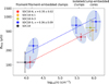 |
Fig. 8 POS magnetic field strength as a function of number density in log-log scale for SDC18-N (red), SDC18-N-1 (orange), SDC18-N- 3 (yellow) and SDC18-S (blue). The data point derived for the entire SDC18 filament is marked in black. Dashed lines are the linear best fits. |
4.4 Relative importance of the magnetic field, gravity, and turbulence from the filament to clumps and to cores
We explore the relative importance of the magnetic field, gravity, and turbulence quantified by the gravitational energy density (uG), magnetic pressure (PB), and turbulent pressure (PT ) and analyze its evolution over the four different scales as introduced in the previous sections. This method is motivated by Tang et al. (2019), who applied it to the three clumps MM1, MM2, and MM3 in the IRDC G34.43+00.24. We defer the comparison with their results to the later part of this section.
The gravitational energy density is derived as
 (12)
(12)
for the SDC18 filament assuming a cylindrical geometry, and as
 (13)
(13)
for SDC18-N and SDC18-S assuming a spherical geometry. The magnetic pressure can be calculated as
 (14)
(14)
Here, we derive the total magnetic field strength (Btotal) from the POS magnetic field strength (Bpos), where we assume  (Crutcher et al. 2004). The factor
  takes into account the statistical averaging of projection effects from 3D onto the 2D POS. The turbulent pressure is estimated as
 (15)
(15)
which assumes that turbulence is isotropic, resulting in the factor 3. All energy densities are derived for the boundaries as defined earlier and listed in the last three columns of Table C.1.
To visualize the evolution of their relative importance, we plot the variation of the three quantities and their ratios as a function of the scales for which they are evaluated in Figure 10. As shown in the left panel of Figure 10, all three quantities are seen to rise when going from large to small scales. This characteristic is also seen in Tang et al. (2019) and expected because they are all functions of density, which increases towards smaller scales. For the ratios measuring their relative importance, we first note that for all four scales and the two clumps, the gravity and magnetic field are more important than turbulence, namely, uG/PT and PB/PT are clearly larger than unity on all scales. This is suggestive of a sub-Alfvénic environment and that turbulence cannot solely prevent gravitational collapse. The relation of gravity and magnetic field is more complicated. At filament and filament-embedded clump scale, the magnetic field dominates over gravity. This is consistent with the morphological interpretation of a strong magnetic field that is dynamically important, as presented in Section 4.3. The evolution of the relative importance then diverges at the isolated clump scale, where SDC18-S continues to be dominated by the magnetic field, while in SDC18-N gravity is dominant. For both SDC18-N and SDC18S, however, uG/PB monotonically increases as the gravitational collapse proceeds and the relative significance of gravity grows toward smaller scales3. At the clump-embedded core scale, the ratio is clearly larger than one in SDC18-N and it is nearly one in SDC18-S. As both clumps will eventually be gravity-dominated, it appears that the transition from magnetic-field-dominated to gravity-dominated can occur in a slower (SDC18-S) or faster (SDC18-N) time frame. Moreover, these possibly different evolutionary paths of the relative importance for these two objects might be linked to their different fragmentation modes, where SDC18-N exhibits an aligned fragmentation pattern, but SDC18S remains highly concentrated (Figure 2). A strong magnetic field can suppress fragmentation as it provides extra support against collapse, creating an isolated massive fragment with no further fragmentation. Indeed, the scaling relation in Figure 8 shows a field strength in SDC18-S about twice larger than in SDC18-N (see also Table C.1), indicating that SDC18-S would be less predisposed to fragmentation. In conclusion, our study of the energy balance suggests a changing relative importance of gravity, magnetic field, and turbulence, further indicating that their interplay at a larger scale can serve as the initial condition of the next level collapse and can affect the outcome of fragmentation on the subsequently smaller scale.
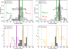 |
Fig. 9 Top: Histograms of the magnetic field position angles (PAs) within the defined boundaries of SDC18-N (left) and SDC18-S (right) at various scales. The gray solid, black solid, and black dashed lines and arrows indicate the circular mean and angular dispersion of the magnetic field at filament-embedded clump (~ 1 pc), isolated clump (~ 0.1 pc), and clump-embedded core (~ 0.01 pc) scale. The solid green line is the circular mean magnetic field orientation over the entire 10 pc filament. The green and red dotted lines mark the PAs of the major axes of the filament and clumps. Bottom: Histograms of the magnetic field PAs in individual clump-embedded cores at 0.01 pc scale from the SMA higher-resolution (~ 1.3ʺ) maps for SDC18-N (left) and SDC18-S (right). Different colors denote different cores marked in Figure 3. The solid and dotted lines mark the circular mean of the magnetic field and the PAs of the cores’ major axes. The angle differences between the mean magnetic field orientations and the major axes of the structures at different scales lie in the range of 90°–100°, signaling the consequence of anisotropic contraction where the B-field regulates the gas motion over multiple scales. The magnetic field also retains its overall mean orientation from filament to clumps and onward to embedded-core scale, with mean PA changes within about 20° to 30° across all scales for both SDC18-N and SDC18-S. Note: all PAs range from 0° to 180°, north to east. 0° and 180° mark identical orientations because of the 0° / 180° ambiguity for circular quantities such as PAs. |
4.5 Comparison with other clumps
The connection between fragmentation and magnetization of clumps has also been observed toward other clouds. Añez-López et al. (2020) studied two hubs (Hub-N and Hub-S) in IRDC G14.225-0.506, which display different fragmentation levels, where Hub-N is more fragmented than Hub-S. Similar to the case presented here, they also find that the less fragmented Hub-S has a higher magnetic field strength (about 0.8 mG) than Hub-N (about 0.2 mG), using the DCF method. Other methods of estimating magnetic field strengths give slightly different results, but magnetic fields stronger by a factor of 4–7 are always obtained for Hub-S. Palau et al. (2021) studied a sample of 18 massive star-forming clumps from the SMA archival polarization data. They find a tentative correlation between the number of fragments and the mass-to-flux ratio of the clumps, while stronger magnetic fields lead to more compact and less massive fragments.
Despite the above findings, the possible trend where stronger magnetic fields lead to less fragmentation might not yet be conclusive. Tang et al. (2019) study three star-forming clumps (MM1, MM2, and MM3) in the IRDC G34.43+00.24 which show different fragmentation modes (“no fragmentation”, “aligned fragmentation”, and “clustered fragmentation”; see Figure 2 in Tang et al. 2019). They performed a similar multiscale energy density analysis of uG, PB, and PT at 2 pc and 0.6 pc. They found an opposite relation between fragmentation and magnetization, as compared to this work. In particular, MM1 is dominated by gravity but displays no further fragmentation. For MM2, the magnetic field is most important despite the cores within it showing an aligned fragmentation parallel to the clump’s major axis and perpendicular to the field lines. The fragments in MM3 appear more clustered, while the contributions of the gravity, magnetic field, and turbulence are comparable. The result in Tang et al. (2019) is consistent with the 3D MHD simulations of clumps undergoing gravitational collapse by Fontani et al. (2016, 2018), which predict that a highly magnetized clump will produce fragments distributed in an aligned morphology.
With the few case studies available at present, it is not yet possible to determine the exact origin(s) of the differences in fragmentation versus relative importance between Tang et al. (2019) and this work. It should be noted that the energy analysis of Tang et al. (2019) and this work is not conducted in completely the same manner. Tang et al. (2019) derived their parameters of clumps at different scales by selecting different sizes of spatial areas in a single data set, while this work utilizes multiple data sets with various resolutions. The selected areas affect the estimates for most of the clump parameters (e.g., M, Reff, nH2 , and Bpos) and can produce systematic uncertainties. Although at filament scale the areas of SDC18-N and SDC18-S are defined by the dendrogram, at the isolated-clump and clumpembedded core scales, they are determined by chosen intensity thresholds of 15σI and 7σI, respectively. To test the robustness of our estimates on the relative importance, we also probed different thresholds: 10σI and 20σI for the isolated-clump scale as well as 3σI and 12σI for the clump-embedded core scale. While the parameters vary by, for instance, 12–30% for the masses and 4–23% for the magnetic field strength, we find that the relative importance among the three constituents for both clumps remains the same. We also find that the relative importance does not change if we exclude the polarization detections between 2σP and 3σP when estimating the magnetic field strengths, although their uncertainties at the clump-embedded core scale become comparable to the field strengths themselves.
One possible factor that might explain the above noted differences in fragmentation versus relative importance is the evolutionary stage of clumps. A commonality between MM2 in G34 and SDC18-N in SDC18, which both show a similar aligned fragmentation pattern, is that they both contain ultracompact HII regions and are the most evolved objects in their parental cloud (Shepherd et al. 2004; Kavak et al. 2021). Ideally, a correlation between fragmentation and evolutionary stage is expected because more fragments can form as time evolves. Observations toward clumps at the very early evolutionary stages discover signs of limited fragmentation from clump to core scale because fragmentation has not yet developed (Csengeri et al. 2017). However, as the source becomes more evolved and hosts active star formation, the feedback from young stellar objects, such as protostellar heating and outflows, may modify the physical environment of the clump and complicate the expected correlation in reality (e.g., Hennebelle et al. 2020; Mathew & Federrath 2021). The comparison of our results with Tang et al. (2019) suggests that there could be additional factors affecting the fragmentation process other than the relative importance of gravity, turbulence, and magnetic field. Further investigations toward more sources will be needed for a more detail study.
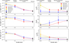 |
Fig. 10 Left panels: uG, PB, and PT as a function of scale on which they are estimated for SDC18-N (red), SDC18-N-1 (orange), SDC18-N-3 (yellow), SDC18-S (blue), and the SDC18 filament (black). Right panels: Ratios of the three quantities uG, PB, and PT as a function of scale. Black dashed lines mark the loci where the ratios are unity, indicating equal contributions of two agents among gravity, magnetic field, and turbulence. We note that the indicated scales on the horizontal axes are assigned numbers. They are meant to represent the scales for the defined boundaries over which the energies are calculated. Error bars indicate 1σ errors propagated through the equations with uncertainties, as described in Section 4.2. |
5 Conclusions
We present a multiscale investigation of the magnetic field toward the filamentary IRDC SDC18 and its two clumps SDC18- N and SDC18-S using polarization observations from the JCMT and the SMA at 850 μm and 1.3 mm. Our observations cover filament (~ 10 pc), filament-embedded clump (~ 1 pc), isolated clump (~ 0.1 pc), and clump-embedded core (~ 0.01 pc) scales, which are crucial for the study of the fragmentation process in high-mass star formation. Along with the continuum polarization observations, our analyses also include gas kinematic information obtained from N2H+ line observations from the IRAM 30m, PdBI, and the SMA, with resolutions similar to the dust continuum polarizarion observations. Our main conclusions are the following:
The JCMT total intensity map depicts the 10 pc long SDC18 filament. The two clumps SDC18-N and SDC18-S appear to be single-peaked but extended in the lower resolution (~ 4ʺ) SMA maps except for the small secondary peak located south-west of the main peak in SDC18-S. The higher- resolution (~ 1.3ʺ) SMA observations display the next level fragmentation. SDC18-N is further fragmented with cores spatially resolved along the major axis of the clump. On the other hand, SDC18-S shows no further fragmentation with its emission mostly concentrated on its main peak. The circular mean magnetic field orientations are perpendicular to the major axes of structures within about 20°or less (filament, filament-embedded clumps, isolated clumps, and clump-embedded cores). To a large extent (>50% of segments) the magnetic field segments at all scales are closely aligned with the circular mean field orientations. The magnetic field dispersion is found to become increasingly larger towards smaller scales.
Larger-scale N2H+ gas kinematics observations from the IRAM 30m and PdBI show a velocity gradient perpendicular to the filament’s major axis and parallel to the prevailing magnetic field orientation. This supports an interpretation where material moves along the magnetic field and can be accreted from the outer diffuse regions to the filament. The direction of the large-scale velocity gradient across the filament is reversed around Dec = – 12°43ʹ00ʹʹ.0, which may be understood a signpost for filament formation via converging flows. The smaller-scale N2H+ data from the SMA show a velocity gradient perpendicular to the outflow axis and magnetic field orientation in SDC18-S.
The observed magnetic field and velocity gradient largely perpendicular to the major axis of the SDC18 filament can be interpreted as a result from either converging flows or filament rotation. In support of a converging-flow scenario, a spectrally narrow, but spatially extended SiO component has been detected toward the central and northern parts of SDC18. The mass accretion rate, estimated from the measured SiO velocity dispersion, suggests that SDC18 would have been able accrete its mass within 0.5–2 Myr, consistently with the typical filament formation timescale. For a filament-rotation scenario, we derived a power-law index of around 1.35 for the specific angular momentum profile across all scales. When isolating the largest scales, a steeper index of 1.9 is found. A varying contribution to velocity gradient and a change in the power-law index is naturally expected in non-head-on converging flow collisions.
We investigated the scaling between density and magnetic field strength from the filament to embedded clumps, isolated clumps, and onward to the clump-embedded cores. Power-law indices of 0.35 and 0.36 are found for SDC18N and SDC18-S, respectively. These are consistent with expectations from a strong-magnetic-field model. A larger magnetic field strength is derived for SDC18-S, which does not appear to fragment further, while a smaller field strength is seen in SDC18-N which is fragmenting into more cores aligned perpendicular to the larger clump-scale magnetic field. The magnetic field also preserves its circular mean orientations within about 20° or less across all scales, while displaying an increasingly larger dispersion towards smaller scales. These features also suggest a strong-magnetic-field scenario, where the field can control the direction of gas flow and the initial direction of a gravitational collapse, until it will be overcome by gravity at a smaller scale. This then leads to the observed growing field dispersion and more complex field morphologies.
A multiscale study of the relative importance of gravity, magnetic field, and turbulence using energy density estimates for the four scales (filament, filament-embedded clumps, isolated clumps, clump-embedded cores) suggests that over all scales and both in SDC18-N and SDC18-S, the gravity and magnetic field are more important than turbulence. As to gravity versus magnetic field, we find that gravity overtakes faster in SDC18-N from the isolated clump scale, while gravity slowly gains over the magnetic field in SDC18-S, approaching equilibrium at the clump-embedded core scale. This faster and slower transition to a gravitydominated regime may explain the different fragmentation outcomes at core scale, with the stronger magnetic field in SDC18-S suppressing fragmentation to a greater extent.
Acknowledgements
This project is supported by the National Science and Technology Council (NSTC) in Taiwan. YWT acknowledges support through NSTC grant NSTC 112-2112-M-001-066 and 111-2112-M-001-064-. PMK acknowledges support from NSTC grants NSTC 113-2112-M-001-016-, NSTC 112-2112-M-001-049-, NSTC 111-2112-M-001-070-, and NSTC 110-2112-M- 001-057-. G.A.F. acknowledges financial support from the State Agency for Research of the Spanish MCIU through the AYA 2017-84390-C2-1-R grant (co-funded by FEDER), through the “Center of Excellence Severo Ochoa” award for the Instituto de Astrofísica de Andalusia (SEV-2017-0709) and grant PID2020-114461GB-I00, funded by MCIN/AEI/10.13039/5011000110. G.A.F. also acknowledges support from the Collaborative Research Centre 956, funded by the Deutsche Forschungsgemeinschaft (DFG) project ID 184018867. The James Clerk Maxwell Telescope is operated by the East Asian Observatory on behalf of The National Astronomical Observatory of Japan; Academia Sinica Institute of Astronomy and Astrophysics; the Korea Astronomy and Space Science Institute; the National Astronomical Research Institute of Thailand; Center for Astronomical Mega-Science (as well as the National Key R&D Program of China with No. 2017YFA0402700). The SMA is a joint project between the Smithsonian Astrophysical Observatory and the Academia Sinica Institute of Astronomy and Astrophysics, and is funded by the Smithsonian Institution and the Academia Sinica. This work is based on observations carried out under project number 054-22 with the IRAM-30m telescope. IRAM is supported by INSU/CNRS (France), MPG (Germany), and IGN (Spain).
References
- André, P., Di Francesco, J., Ward-Thompson, D., et al. 2014, in Protostars and Planets VI, eds. H. Beuther, R. S. Klessen, C. P. Dullemond, & T. Henning, 27 [Google Scholar]
- Añez-López, N., Busquet, G., Koch, P. M., et al. 2020, A&A, 644, A52 [NASA ADS] [CrossRef] [EDP Sciences] [Google Scholar]
- Armijos-Abendaño, J., Banda-Barragán, W. E., Martín-Pintado, J., et al. 2020, MNRAS, 499, 4918 [Google Scholar]
- Balfour, S. K., Whitworth, A. P., & Hubber, D. A. 2017, MNRAS, 465, 3483 [NASA ADS] [CrossRef] [Google Scholar]
- Beckwith, S. V. W., Sargent, A. I., Chini, R. S., & Guesten, R. 1990, AJ, 99, 924 [Google Scholar]
- Belloche, A. 2013, in EAS Publications Series, 62, eds. P. Hennebelle, & C. Charbonnel, 25 [Google Scholar]
- Bergin, E. A., & Tafalla, M. 2007, ARA&A, 45, 339 [Google Scholar]
- Beuther, H., & Steinacker, J. 2007, ApJ, 656, L85 [NASA ADS] [CrossRef] [Google Scholar]
- Beuther, H., Schilke, P., Menten, K. M., et al. 2002, ApJ, 566, 945 [Google Scholar]
- Beuther, H., Henning, T., Linz, H., et al. 2010, A&A, 518, L78 [NASA ADS] [CrossRef] [EDP Sciences] [Google Scholar]
- Beuther, H., Ragan, S. E., Johnston, K., et al. 2015, A&A, 584, A67 [NASA ADS] [CrossRef] [EDP Sciences] [Google Scholar]
- Chandrasekhar, S., & Fermi, E. 1953, ApJ, 118, 116 [Google Scholar]
- Chapin, E. L., Berry, D. S., Gibb, A. G., et al. 2013, MNRAS, 430, 2545 [Google Scholar]
- Chen, H.-R. V., Zhang, Q., Wright, M. C. H., et al. 2019, ApJ, 875, 24 [Google Scholar]
- Chen, C.-Y., Mundy, L. G., Ostriker, E. C., Storm, S., & Dhabal, A. 2020, MNRAS, 494, 3675 [Google Scholar]
- Ching, T.-C., Lai, S.-P., Zhang, Q., et al. 2017, ApJ, 838, 121 [Google Scholar]
- Clapham, C., Nicholson, J., & Nicholson, J. 2014, The Concise Oxford Dictionary of Mathematics, Oxford Paperback Reference (OUP Oxford) [Google Scholar]
- Clarke, S. D., Whitworth, A. P., Duarte-Cabral, A., & Hubber, D. A. 2017, MNRAS, 468, 2489 [Google Scholar]
- Clarke, S. D., Whitworth, A. P., Spowage, R. L., et al. 2018, MNRAS, 479, 1722 [Google Scholar]
- Commerçon, B., Hennebelle, P., & Henning, T. 2011, ApJ, 742, L9 [CrossRef] [Google Scholar]
- Cosentino, G., Jiménez-Serra, I., Henshaw, J. D., et al. 2018, MNRAS, 474, 3760 [NASA ADS] [Google Scholar]
- Cosentino, G., Jiménez-Serra, I., Henshaw, J. D., et al. 2020, MNRAS, 499, 1666 [NASA ADS] [CrossRef] [Google Scholar]
- Crutcher, R. M., Nutter, D. J., Ward-Thompson, D., & Kirk, J. M. 2004, ApJ, 600, 279 [Google Scholar]
- Csengeri, T., Bontemps, S., Wyrowski, F., et al. 2017, A&A, 600, L10 [NASA ADS] [CrossRef] [EDP Sciences] [Google Scholar]
- Davis, L. 1951, Phys. Rev., 81, 890 [Google Scholar]
- Fallscheer, C., Beuther, H., Zhang, Q., Keto, E., & Sridharan, T. K. 2009, A&A, 504, 127 [NASA ADS] [CrossRef] [EDP Sciences] [Google Scholar]
- Federrath, C., Krumholz, M., & Hopkins, P. F. 2017, in Journal of Physics Conference Series, 837, 012007 [Google Scholar]
- Fontani, F., Commerçon, B., Giannetti, A., et al. 2016, A&A, 593, L14 [NASA ADS] [CrossRef] [EDP Sciences] [Google Scholar]
- Fontani, F., Commerçon, B., Giannetti, A., et al. 2018, A&A, 615, A94 [NASA ADS] [CrossRef] [EDP Sciences] [Google Scholar]
- Friberg, P., Bastien, P., Berry, D., et al. 2016, SPIE Conf. Ser., 9914, 991403 [Google Scholar]
- Gibb, A. G., Davis, C. J., & Moore, T. J. T. 2007, MNRAS, 382, 1213 [Google Scholar]
- Ginsburg, A., & Mirocha, J. 2011, PySpecKit: Python Spectroscopic Toolkit, Astrophysics Source Code Library [record ascl:1109.001] [Google Scholar]
- Goldsmith, P. F., & Arquilla, R. 1985, in Protostars and Planets II, eds. D. C. Black, & M. S. Matthews, 137 [Google Scholar]
- Goodman, A. A., Benson, P. J., Fuller, G. A., & Myers, P. C. 1993, ApJ, 406, 528 [Google Scholar]
- Hacar, A., Tafalla, M., & Alves, J. 2017, A&A, 606, A123 [NASA ADS] [CrossRef] [EDP Sciences] [Google Scholar]
- Hacar, A., Clark, S. E., Heitsch, F., et al. 2023, in Astronomical Society of the Pacific Conference Series, 534, Protostars and Planets VII, eds. S. Inutsuka, Y. Aikawa, T. Muto, K. Tomida, & M. Tamura, 153 [Google Scholar]
- Heitsch, F. 2013, ApJ, 769, 115 [Google Scholar]
- Hennebelle, P., Commerçon, B., Joos, M., et al. 2011, A&A, 528, A72 [NASA ADS] [CrossRef] [Google Scholar]
- Hennebelle, P., Commerçon, B., Lee, Y.-N., & Chabrier, G. 2020, ApJ, 904, 194 [NASA ADS] [CrossRef] [Google Scholar]
- Hildebrand, R. H., Dragovan, M., & Novak, G. 1984, ApJ, 284, L51 [NASA ADS] [CrossRef] [Google Scholar]
- Houde, M., Vaillancourt, J. E., Hildebrand, R. H., Chitsazzadeh, S., & Kirby, L. 2009, ApJ, 706, 1504 [Google Scholar]
- Howard, C. S., Pudritz, R. E., & Harris, W. E. 2016, MNRAS, 461, 2953 [Google Scholar]
- Hull, C. L. H., & Zhang, Q. 2019, Front. Astron. Space Sci., 6, 3 [Google Scholar]
- Jiménez-Serra, I., Caselli, P., Tan, J. C., et al. 2010, MNRAS, 406, 187 [Google Scholar]
- Kavak, Ü., Sánchez-Monge, Á., López-Sepulcre, A., et al. 2021, A&A, 645, A29 [NASA ADS] [CrossRef] [EDP Sciences] [Google Scholar]
- Kim, W. J., Urquhart, J. S., Veena, V. S., et al. 2023, A&A, 679, A123 [NASA ADS] [CrossRef] [EDP Sciences] [Google Scholar]
- Lazarian, A., & Hoang, T. 2007, MNRAS, 378, 910 [Google Scholar]
- Li, H.-B., Yuen, K. H., Otto, F., et al. 2015, Nature, 520, 518 [Google Scholar]
- Lin, Y., Wyrowski, F., Liu, H. B., et al. 2022, A&A, 658, A128 [NASA ADS] [CrossRef] [EDP Sciences] [Google Scholar]
- Liu, T., Evans, N. J., Kim, K.-T., et al. 2020, MNRAS, 496, 2790 [Google Scholar]
- Liu, M., Tan, J. C., Marvil, J., et al. 2021, ApJ, 921, 96 [NASA ADS] [CrossRef] [Google Scholar]
- Louvet, F., Motte, F., Gusdorf, A., et al. 2016, A&A, 595, A122 [NASA ADS] [CrossRef] [EDP Sciences] [Google Scholar]
- Lu, X., Zhang, Q., Liu, H. B., Wang, J., & Gu, Q. 2014, ApJ, 790, 84 [NASA ADS] [CrossRef] [Google Scholar]
- Marsh, K. A., Whitworth, A. P., Lomax, O., et al. 2017, MNRAS, 471, 2730 [Google Scholar]
- Mathew, S. S., & Federrath, C. 2021, MNRAS, 507, 2448 [CrossRef] [Google Scholar]
- McKee, C. F., & Ostriker, E. C. 2007, ARA&A, 45, 565 [Google Scholar]
- Mouschovias, T. C. & Ciolek, G. E. 1999, in NATO Advanced Study Institute (ASI) Series C, 540, The Origin of Stars and Planetary Systems, eds. C. J. Lada, & N. D. Kylafis, 305 [Google Scholar]
- Ostriker, E. C., Stone, J. M., & Gammie, C. F. 2001, ApJ, 546, 980 [Google Scholar]
- Palau, A., Zhang, Q., Girart, J. M., et al. 2021, ApJ, 912, 159 [NASA ADS] [CrossRef] [Google Scholar]
- Pattle, K., Fissel, L., Tahani, M., Liu, T., & Ntormousi, E. 2023, in Astronomical Society of the Pacific Conference Series, 534, Protostars and Planets VII, eds. S. Inutsuka, Y. Aikawa, T. Muto, K. Tomida, & M. Tamura, 193 [Google Scholar]
- Pattle, K., Fissel, L., Tahani, M., Liu, T., & Ntormousi, E. 2022, [arXiv:2203.11179] [Google Scholar]
- Peretto, N., & Fuller, G. A. 2009, A&A, 505, 405 [NASA ADS] [CrossRef] [EDP Sciences] [Google Scholar]
- Peretto, N., & Fuller, G. A. 2010, ApJ, 723, 555 [NASA ADS] [CrossRef] [Google Scholar]
- Peretto, N., Gaudel, M., Louvet, F., et al. 2015, in EAS Publications Series, 75, 167 [CrossRef] [EDP Sciences] [Google Scholar]
- Pineda, J. E., Arzoumanian, D., André, P., et al. 2023, in Protostars and Planets VII, eds. S. Inutsuka, Y. Aikawa, T. Muto, K. Tomida, & M. Tamura, Astronomical Society of the Pacific Conference Series, 534, 233 [NASA ADS] [Google Scholar]
- Planck Collaboration Int. XLII 2016, A&A, 596, A103 [NASA ADS] [CrossRef] [EDP Sciences] [Google Scholar]
- Primiani, R. A., Young, K. H., Young, A., et al. 2016, J. Astron. Instrum., 5, 1641006 [NASA ADS] [CrossRef] [Google Scholar]
- Ragan, S. E., Bergin, E. A., & Wilner, D. 2011, ApJ, 736, 163 [NASA ADS] [CrossRef] [Google Scholar]
- Rathborne, J. M., Longmore, S. N., Jackson, J. M., et al. 2015, ApJ, 802, 125 [Google Scholar]
- Rosolowsky, E. W., Pineda, J. E., Kauffmann, J., & Goodman, A. A. 2008, ApJ, 679, 1338 [Google Scholar]
- Russeil, D., Tigé, J., Adami, C., et al. 2016, A&A, 587, A135 [NASA ADS] [CrossRef] [EDP Sciences] [Google Scholar]
- Sánchez-Monge, Á., López-Sepulcre, A., Cesaroni, R., et al. 2013, A&A, 557, A94 [NASA ADS] [CrossRef] [EDP Sciences] [Google Scholar]
- Sanhueza, P., Jackson, J. M., Zhang, Q., et al. 2017, ApJ, 841, 97 [Google Scholar]
- Sault, R. J., Teuben, P. J., & Wright, M. C. H. 1995, in Astronomical Society of the Pacific Conference Series, 77, Astronomical Data Analysis Software and Systems IV, eds. R. A. Shaw, H. E. Payne, & J. J. E. Hayes, 433 [Google Scholar]
- Schilke, P., Walmsley, C. M., Pineau des Forets, G., & Flower, D. R. 1997, A&A, 321, 293 [NASA ADS] [Google Scholar]
- Schneider, N., Csengeri, T., Bontemps, S., et al. 2010, A&A, 520, A49 [CrossRef] [EDP Sciences] [Google Scholar]
- Shepherd, D. S., Nürnberger, D. E. A., & Bronfman, L. 2004, ApJ, 602, 850 [Google Scholar]
- Sridharan, T. K., Beuther, H., Schilke, P., Menten, K. M., & Wyrowski, F. 2002, ApJ, 566, 931 [Google Scholar]
- Tackenberg, J., Beuther, H., Henning, T., et al. 2014, A&A, 565, A101 [NASA ADS] [CrossRef] [EDP Sciences] [Google Scholar]
- Tang, Y.-W., Koch, P. M., Peretto, N., et al. 2019, ApJ, 878, 10 [Google Scholar]
- Tatematsu, K., Ohashi, S., Sanhueza, P., et al. 2016, PASJ, 68, 24 [NASA ADS] [CrossRef] [Google Scholar]
- Wang, J.-W., Koch, P. M., Tang, Y.-W., et al. 2022, ApJ, 931, 115 [NASA ADS] [CrossRef] [Google Scholar]
- Williams, G. M., Peretto, N., Avison, A., Duarte-Cabral, A., & Fuller, G. A. 2018, A&A, 613, A11 [NASA ADS] [CrossRef] [EDP Sciences] [Google Scholar]
Appendix A Polarization
A map of the detected JCMT/POL-2 polarization orientations, scaled with their percentages, is shown in Figure A.1. We apply a threshold I > 5σI and P > 2σP when selecting polarized emission. The unweighted mean and median polarization percentages are 6.2% and 5.0% with a standard deviation, maximum and minimum of 4.7%, 27.9%, and 0.5%, respectively. The blue segments in Figure A.1 denote polarization detections with P > 3σP, while green segments are detections with 3σP > P > 2σP. Besides the main filament SDC18 located in the centre of the map, Figure A.1 further reveals two smaller clouds in its north-west and several minor structures scattered within the field-of-view of the JCMT observations.
Figure A.2 shows the observed polarization percentage, P, as a function of the total intensity I for both the JCMT and SMA data. A linear fit in log-log space yields a power-law index α = – 0.86 0.02 for P ∝ Iα for the 10 pc filament revealed with the JCMT/POL-2. From the SMA data, α of SDC- 18N is −0.89 ± 0.06 and −0.90 ± 0.05, and −0.53 ± 0.06 and −0.86 ± 0.08 for SDC18-S, for the coarser 4ʹʹ.41 × 3ʹʹ.32 and higher resolution 1ʹʹ.45 × 1ʹʹ.25 observations, respectively.
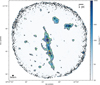 |
Fig. A.1 JCMT total intensity Stokes I map overlaid with polarization segments at 850 μm over the entire field of view (11’) of the JCMT. Blue segments show the polarization orientations with I > 5σI and P > 3σP, while green segments are I > 5σI and 3σP > P > 2σP. The lengths of the segments are proportional to |

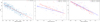 |
Fig. A.2 Polarization fraction as a function of total intensity for JCMT POL-2 data (left panel), lower-resolution (4ʺ) SMA data (middle panel) and higher-resolution (1.3ʺ) SMA data (right panel). The data are selected with I > 5σI and P > 2σP. Solid lines are linear fits in log-log space with power-law indices given in the legends. |
Appendix B Structure function
Table B.1 lists the parameters derived from the structure function analysis at each scale. The resulting structure function as a function of distance l with the best fits are shown in the top panels of Figure B.1. Additionally, the turbulent correlated components of the structure function are shown in the bottom panels of Figure B.1. At 1 pc scale, the structure function fit fails because (statistically) there are not enough segments and morphologically the segments are highly uniformly distributed within the boundary of clumps we defined for the 1 pc scale, such that the large-scale components are not present in the observed structure functions. It has been tested in simulations that the availability of the structure function fit closely depends on the existence of the large-scale ordered components which appear as plateaus or shallow slopes at large l after the turnover from steadily increasing turbulent correlated component at small l. In simulation, the fitted parameters of the structure function become highly fluctuate even with a small change of the structure function profiles in absence of the large-scale component. A more detailed test on the application of the structure function analysis will be presented in a forthcoming paper (Clarke et al. in prep.).
Structure function fit parameters.
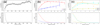 |
Fig. B.1 Top panels: Magnetic field structure functions as a function of distance l of SDC18 (black) at filament scale (black) in panel (a), and of SDC18-N (red) and SDC18-S (blue) at isolated clump scale in panel (b), and of SDC18-N-1 (orange), SDC18-N-3 (yellow) and SDC18-S-1 (cyan) at clump-embedded core scale in panel (c). Solid lines are the best fits of Equation 10. Dashed lines show the ordered component ( |


Appendix C Parameters across multiple scales in SDC18
Parameters across multiple scales in SDC18.
Note: the rotation axes of the structures at various scales might have different inclination angles, and the projection effects are not taken into account in the specific angular momentum profile.
Note: the estimated Bpos strength using DCF methods tends to be larger than the measured field strength along the LOS using Zeeman measurements (see recent review by Pattle et al. 2022). However, due to the large scatter in both Zeeman and DCF measurements at a given density, no quantitative estimate or correction has yet been attempted. Assuming that the Zeeman estimate is the ‘true’ field strength, a systematic down-scatter from this value by a factor of 2 or 3 will yield a factor 4 to possibly 10 smaller energy estimates (PB B2). While this will bring the related curves down in Figure 10 (and, e.g., uG/PB will transition earlier across 1 for SDC18-S), the overall relative trends will remain.
All Tables
All Figures
|
Fig. 1 Spitzer images of SDC18 at 24 μm (red), 8 μm (green), and 5.8 μm (blue), together with JCMT/POL-2 850μm dust continuum contours (left panel) and magnetic field structures (right panel). The contours denote the 50, 500, and 1000 mJy beam−1 of the JCMT total intensity. Orange contours are the boundaries of SDC18-N and SDC18-S at filament-embedded clump scale determined by the dendrogram analysis. The JCMT/POL-2 magnetic field orientations with P> 3σP are in yellow and in red for 3σP > P > 2σP. White segments are the larger-scale Planck magnetic field orientations inferred from 90° rotation of polarization at 353 GHz (∼ 5ʹ) in a pixel size of 103ʺ. |
| In the text | |
|
Fig. 2 (a): SDC18 continuum emission at 850 μm with an angular resolution of 14.6ʺ with JCMT/POL-2 in contours and magnetic field segments, capturing the entire filament and the filament-embedded clumps, SDC18-N and SDC18-S (green boxes), zoomed in the middle and right panels. The contours are 50, 500, and 1000 mJy beam−1. (b), (c): Continuum emission at 1.3 mm in contours and magnetic field segments of SDC18-N (b) and SDC18-S (c) with an angular resolution of 4.41ʺ × 3.32ʺ with the SMA, capturing the isolated clumps resolving out diffuser and more extended emission. Solid black contours represent the Stokes I flux levels at 15, 40, and 80σI, while dashed black contours show -5σI. (d), (e): The same as the middle panels but with an angular resolution of 1.45ʺ × 1.25ʺ, capturing the clump-embedded cores revealing fragmentation of the larger clump. Solid black contours are 7, 30, and 45σI Stokes I flux levels, while dashed black contours are -7σI. The segments in all panels show magnetic field orientations with P > 3σP detections in blue and 3σP > P > 2σP detections in red. The right panels display magnetic field segments gridded at half of the synthesized beam resolution. The segments in the middle panels are overgridded for a sharper visualization, but only data at half of the synthesized beam are used for the further analysis. |
| In the text | |
|
Fig. 3 Circular mean magnetic field orientations in different regions and scales of SDC18. The black segments in panel (a) show the magnetic field orientations averaged within boxes of 100ʺ × 100ʺ along the filament ridge, overplotted on the JCMT continuum map. The intersection angles of the grey segments are the dispersion values of the field orientations. The locations of the segments are the average locations of the detected polarization signals within each box. The purple segment and intersection angle of the violet segments show the overall circular mean of 115° with its dispersion of 45° of the magnetic field orientations within the entire filament. The red and green segments in all panels present the mean magnetic field orientations and position angles of the major axes for the clumps and cores at different scales. Magenta contours mark the boundaries of the individual cores in the SMA 1.3ʺ resolution maps for SDC18-N (panel (d)) and SDC18-S (panel (e)) identified in Section 3.2. |
| In the text | |
|
Fig. 4 SDC18 N2H+ centroid velocity and dispersion maps at various scales. Panels (a) and (b) show the IRAM-30m N2H+ (1–0) centroid velocity and velocity dispersion map with a resolution of 27ʺ. The black dashed line in the first panel marks Dec = – 12°43ʹ00ʹʹ.0 where the direction of the velocity gradient flips. Panels (c) and (d) are the N2H+ (1–0) centroid velocity and velocity dispersion map with a beam size of 5.77ʺ × 3.39ʺ from the PdBI. Panels (e) and (f) are the N2H+ (3–2) centroid velocity and velocity dispersion map of SDC18-S observed by the SMA with a beam size of 2.28ʺ × 1.11ʺ. The same black contours representing JCMT total intensity levels at 50, 500, and 1000 mJy beam−1, identical to the left panel of Figure 2, are shown in the first four panels. The SMA total intensity contours of 7, 30, and 45σ (identical to the lower right panel of Figure 2) are shown in the two maps on the very right. In panel (e), a black dot and arrow mark the continuum peak and the outflow orientation in SDC18-S reported by Fallscheer et al. (2009). |
| In the text | |
|
Fig. 5 Histogram (left panel) and map (right panel) of absolute differences in position angles between magnetic field orientations and velocity gradients. The black contours are the same JCMT total intensity levels at 50, 500, and 1000 mJy beam−1, as in the left panel of Figure 2. |
| In the text | |
|
Fig. 6 Left: SDC18 SiO (2–1) integrated intensity map from the IRAM-30m. The 3σ intensity level is marked by the black contour. Red contours show the same JCMT total intensity levels of 50, 500, and 1000 mJy/beam as in panel (a) in Figure 2. Right: Spectra extracted from several positions marked by the black dashed lines. In the upper two panels, the red lines are the single-Gaussian fits, while in the bottom panel, the red line is the combination of a two-component Gaussian fit including a broader and narrower component in green and blue, respectively. |
| In the text | |
|
Fig. 7 Radial profile of specific angular momentum for SDC18 from N2H+ observations covering different scales. |
| In the text | |
|
Fig. 8 POS magnetic field strength as a function of number density in log-log scale for SDC18-N (red), SDC18-N-1 (orange), SDC18-N- 3 (yellow) and SDC18-S (blue). The data point derived for the entire SDC18 filament is marked in black. Dashed lines are the linear best fits. |
| In the text | |
|
Fig. 9 Top: Histograms of the magnetic field position angles (PAs) within the defined boundaries of SDC18-N (left) and SDC18-S (right) at various scales. The gray solid, black solid, and black dashed lines and arrows indicate the circular mean and angular dispersion of the magnetic field at filament-embedded clump (~ 1 pc), isolated clump (~ 0.1 pc), and clump-embedded core (~ 0.01 pc) scale. The solid green line is the circular mean magnetic field orientation over the entire 10 pc filament. The green and red dotted lines mark the PAs of the major axes of the filament and clumps. Bottom: Histograms of the magnetic field PAs in individual clump-embedded cores at 0.01 pc scale from the SMA higher-resolution (~ 1.3ʺ) maps for SDC18-N (left) and SDC18-S (right). Different colors denote different cores marked in Figure 3. The solid and dotted lines mark the circular mean of the magnetic field and the PAs of the cores’ major axes. The angle differences between the mean magnetic field orientations and the major axes of the structures at different scales lie in the range of 90°–100°, signaling the consequence of anisotropic contraction where the B-field regulates the gas motion over multiple scales. The magnetic field also retains its overall mean orientation from filament to clumps and onward to embedded-core scale, with mean PA changes within about 20° to 30° across all scales for both SDC18-N and SDC18-S. Note: all PAs range from 0° to 180°, north to east. 0° and 180° mark identical orientations because of the 0° / 180° ambiguity for circular quantities such as PAs. |
| In the text | |
|
Fig. 10 Left panels: uG, PB, and PT as a function of scale on which they are estimated for SDC18-N (red), SDC18-N-1 (orange), SDC18-N-3 (yellow), SDC18-S (blue), and the SDC18 filament (black). Right panels: Ratios of the three quantities uG, PB, and PT as a function of scale. Black dashed lines mark the loci where the ratios are unity, indicating equal contributions of two agents among gravity, magnetic field, and turbulence. We note that the indicated scales on the horizontal axes are assigned numbers. They are meant to represent the scales for the defined boundaries over which the energies are calculated. Error bars indicate 1σ errors propagated through the equations with uncertainties, as described in Section 4.2. |
| In the text | |
|
Fig. A.1 JCMT total intensity Stokes I map overlaid with polarization segments at 850 μm over the entire field of view (11’) of the JCMT. Blue segments show the polarization orientations with I > 5σI and P > 3σP, while green segments are I > 5σI and 3σP > P > 2σP. The lengths of the segments are proportional to |
| In the text | |
|
Fig. A.2 Polarization fraction as a function of total intensity for JCMT POL-2 data (left panel), lower-resolution (4ʺ) SMA data (middle panel) and higher-resolution (1.3ʺ) SMA data (right panel). The data are selected with I > 5σI and P > 2σP. Solid lines are linear fits in log-log space with power-law indices given in the legends. |
| In the text | |
|
Fig. B.1 Top panels: Magnetic field structure functions as a function of distance l of SDC18 (black) at filament scale (black) in panel (a), and of SDC18-N (red) and SDC18-S (blue) at isolated clump scale in panel (b), and of SDC18-N-1 (orange), SDC18-N-3 (yellow) and SDC18-S-1 (cyan) at clump-embedded core scale in panel (c). Solid lines are the best fits of Equation 10. Dashed lines show the ordered component ( |
| In the text | |
Current usage metrics show cumulative count of Article Views (full-text article views including HTML views, PDF and ePub downloads, according to the available data) and Abstracts Views on Vision4Press platform.
Data correspond to usage on the plateform after 2015. The current usage metrics is available 48-96 hours after online publication and is updated daily on week days.
Initial download of the metrics may take a while.