| Issue |
A&A
Volume 695, March 2025
|
|
|---|---|---|
| Article Number | A37 | |
| Number of page(s) | 29 | |
| Section | Planets, planetary systems, and small bodies | |
| DOI | https://doi.org/10.1051/0004-6361/202452328 | |
| Published online | 03 March 2025 | |
Photometric modelling of self-gravity wakes and overstable oscillations in Saturn’s rings
Space Physics and Astronomy Research unit, University of Oulu,
90014
Oulu,
Finland
★ Corresponding author; heikki.salo@oulu.fi
Received:
20
September
2024
Accepted:
23
December
2024
Context. We present a detailed survey of the effect of various dynamical parameters on the photometric properties of Saturn’s rings. Our numerical simulations include the mutual impacts and self-gravity of particles and cover the range of parameters leading to axisymmetric viscous overstabilities and/or trailing self-gravity wake structures.
Aims. Our goal is to place constraints on the physical parameters of ring particles (internal density, ρ, elasticity, ϵn, size distribution width, W), based on a comparison with Hubble Space Telescope observations of the ring’s azimuthal brightness asymmetry. The best fit models are also compared to B and A ring opacity and viscosity measurements.
Methods. Photometric modelling uses Monte Carlo (MC) ray tracing of simulated particle fields. Dynamical simulations are performed in a message passage interface (MPI) environment with the novel SoftIS code, which incorporates the treatment of impacts in terms of visco-elastic forces with a Rebound code using tree-based gravity calculation. Besides fully self-gravitating simulations, we performed simulations in which self-consistent planar gravity was combined with an enhanced frequency of vertical oscillations, Ωz/Ω > 1. Such ‘hybrid’ simulations mimic additional sticking forces in the sense that they lead to vertically more flattened self-gravity wake structures.
Results. Our models demonstrate the close correspondence between the strength of wake structures, measured by gravitational viscosity, and the amplitude of azimuthal variations in brightness, I/F, and optical depth, τphot. Trailing self-gravity wakes connect to I/F and τphot minima ~20° before the ansae, where the wakes are viewed along their long axis. No abrupt change in asymmetry amplitude is seen between overstability- or wake-dominated systems. The clearest sign of axisymmetric overstability is the shift in the longitude of minimum towards ring ansae. In the weak gravity regime, the simulated minimum can occur even after the ring ansa, due to the presence of shear-induced leading density enhancements; however, the associated amplitude is a few percents at most and is thus hidden if wakes or overstabilities are present. Our models emphasise the importance of size distribution: in the weak gravity regime, the inclusion of an extended size distribution shifts an overstable system to a wake-dominated one, as self-gravity becomes more effective due to the increased filling factor inside the wakes. In the case of strong gravity, size distribution reduces the asymmetry amplitude, the more uniformly distributed small particles partially hiding the wakes, which however remain dynamically strong among large particles. The best overall match to various observations is obtained with extended size distribution models, for ρ ~ 250 kg m−3; however, hybrid models leading to flatter and thus weaker wakes can match larger ρ better.
Conclusions. Size distribution models with self-gravity and inelastic collisions can match the constraints set by azimuthal brightness asymmetry, and reproduce well the A and B ring opacity versus elevation profiles. However, models that include only self-gravity forces indicate very low internal density of particles. Additional sticking forces, in this study mimicked as extra vertical compression, are thus likely to be important, allowing for an internal density closer to the solid ice density. Photometric comparisons similar to the ones in the current study but based on simulations including realistic sticking forces are clearly needed.
Key words: methods: numerical / planets and satellites: rings
© The Authors 2025
 Open Access article, published by EDP Sciences, under the terms of the Creative Commons Attribution License (https://creativecommons.org/licenses/by/4.0), which permits unrestricted use, distribution, and reproduction in any medium, provided the original work is properly cited.
This article is published in open access under the Subscribe to Open model. Subscribe to A&A to support open access publication.
1 Introduction
Self-gravity wakes – the transient local density enhancements caused by the competition between the ring particles’ mutual gravity and the orbital shear (Salo 1992; Toomre & Kalnajs 1991; Salo 1995) – manifest in several ways in observations of Saturn’s rings. This stems from the systematic orientation that wakes have with respect to local orbital motion (trailing on average by about 20°), so that even if individual wakes, rapidly forming and dissolving filamentary structures ranging from a few tens of metres to a hundred metres in scale, are too small to be resolved in direct images, they can yield a global signature affecting the amount of sunlight reflected and transmitted by the rings. Most importantly, they explain the A-ring azimuthal brightness asymmetry, the appearance of bi-symmetric brightness minima at ~20° before ring ansae, which was already being discovered and analysed in the pre-mission era (Camichel 1958; Colombo et al. 1976; Lumme et al. 1977; Thompson et al. 1981) before being more quantitatively assessed from the Voyager flyby-images, both in transmitted (Franklin et al. 1987) and in reflected light (Dones et al. 1993). A thorough study of reflected light asymmetry was performed by French et al. (2007) using an extensive Hubble Space Telescope (HST) dataset covering the full range of observing geometries accessible from Earth. A representative sub-image of the east ansa of Saturn’s rings, which was analysed in that study, is shown in Fig. 1.
Besides brightness variations, the presence of self-gravity wakes was also deduced from Arecibo radar observations (Nicholson et al. 2005) and from observations of Saturn’s microwave radiation transmitted through the rings (Dunn et al. 2004). In both French et al. (2007) and Nicholson et al. (2005), a weaker asymmetry was also observed in the B ring. However, the most detailed picture of self-gravity wakes has been provided by the ring opacity profiles from Cassini Ultraviolet Imaging Spectograph (UVIS) and Visual and Infrared Mapping Spectrometer (VIMS) stellar occultations (Colwell et al. 2006, 2007; Hedman et al. 2007; Jerousek et al. 2016), Radio Science Subsystem (RSS) radio occultation measurements (Thomson et al. 2007), and UVIS Solar occultations (Jarmak et al. 2022). According to these observations, wakes are present practically everywhere in the A and B rings, wherever the ring is sufficiently transparent for a signal to be detected. Moreover, the good resolution of the occultation measurements makes it possible to resolve individual wakes (Jerousek et al. 2024). Wakes also manifest in Cassini Composite Infrared Spectrometer (CIRS) thermal emission measurements (Ferrari et al. 2009; Morishima et al. 2014).
While the presence of self-gravity wakes has been inferred from many type of observations, the evidence for viscous overstabilities is sparser. Viscous overstability, in the form of spontaneous growth of axisymmetric oscillations (Schmit & Tscharnuter 1995; Schmidt et al. 2001; Schmidt & Salo 2003; Latter & Ogilvie 2008; Schmidt et al. 2009) arises naturally in N-body simulations in a similar manner to self-gravity wakes, although compared to wakes, the parameter range leading to overstability is narrower, requiring a high impact frequency and moderately weak self-gravity (Salo et al. 2001). Like self-gravity wakes, overstable oscillations lead to a longitude-dependent brightness of the rings, but due to their axisymmetric nature the expected longitude of minimum brightness is shifted towards ring ansae (in ground-based geometries). According to simulations, the axisymmetric oscillations may co-exist with the inclined self-gravity wake structures, a combination that can lead to complicated photometric behaviour as a function of illumination and viewing geometries.
Regular axisymmetric density undulations with 100–200 metre radial wavelengths have been detected in the occultation profiles of the inner A ring (Thomson et al. 2007; Colwell et al. 2007; Hedman et al. 2007) and in several locations in the B ring, including the inner edge of the B ring. Observations by Hedman et al. (2014) indicate that the structures maintain their azimuthal coherence over thousands of kilometres, supporting their interpretation as axisymmetric overstable oscillations. The maximum distance at which overstability is detected (~ 124 000 km) provides an important constraint for the strength of self-gravity in the B and A rings. There is also indirect evidence for the interplay of wakes and overstability: the pitch angle assigned for self-gravity wakes from UVIS occultation observations is closer to tangential in the outer B ring (Colwell et al. 2007), compared to what would be expected for pure self-gravity wakes. A similar trend is seen in the minimum longitude of HST reflected light observations (French et al. 2007). Very recently, Jerousek et al. (2024) have directly demonstrated the co-existence of wakes and overstability in the inner A-ring region, by conducting an auto-correlation analysis utilising multiple UVIS stellar occultation profiles.
The comparison of the extensive above-mentioned HST dataset to the predictions of N-body models provided a good match to many observed characteristics of azimuthal asymmetry (French et al. 2007). The modelling was based on Monte Carlo (MC) ray tracing of particle fields obtained from dynamical simulations, calculated for a few representative distances and optical depths in Saturn’s rings (Salo & Karjalainen 2003; Salo et al. 2004). For example, the models in French et al. (2007) accounted well for the observed elevation angle dependence of the A-ring brightness asymmetry, with maximum amplitude at elevation B ~ 10° – 15°, corresponding to the maximum contrast between the visibility of bright wakes and rarefied inter-wake regions. Likewise, the small shifts in the observed location of the minimum, depending on the Sun and observer longitudes, were well matched. However, what remained puzzling was the fact that while simple identical particle models seem to agree very well with the longitude of minimum brightness, the presumably more realistic models with a size distribution (with range of 10 in radii) clearly yielded a worse agreement. Likewise, although dynamical models assuming porous ice particles with an internal density of around 450 kg m−3 were able to account for both a strong asymmetry in the A ring (with ±25% brightness variations) and a much weaker asymmetry in the B ring (±5%), the observed rapid rise in amplitude from the inner to mid A ring and the similar decline towards the outer A ring remained a mystery. This asymmetry peak was originally discovered in Voyager data (Dones et al. 1993) and was fully confirmed by HST observations (French et al. 2007).
Compared to the pre-2007 N-body simulations, we can now use nearly two orders of more particles (N ~ 106 instead of 104), which allows one to model higher dynamical optical depths and more extended size distributions than the ones explored in French et al. (2007). To achieve this, we used the recently developed SoftIS-code (Mondino-Llermanos & Salo 2022; Mondino-Llermanos & Salo 2023). This code is based on the public domain REBOUND-code (Rein & Liu 2012) and works in a multi-processor environment. The advantage of SoftIS is its description of impacts with a linear visco-elastic force model (Salo 1995), which makes it possible to simulate dense and strongly self-gravitating systems in which it becomes increasingly difficult to describe the evolution as a sequence of well-separated binary impacts. For example, SoftIS can be used to study gravitational accretion in instances in which the traditional instantaneous impact method fails (Mondino-Llermanos & Salo 2022).
Our goal is to present a reasonably thorough study of the photometric consequences of self-gravity wakes and axisymmetric viscous oscillations, based on the newly extended simulations, while using the same photometric methods as in French et al. (2007). Section 2 describes our dynamical and photometric simulation methods, while Sect. 3 illustrates how wakes and overstabilities are expected to affect the ring observations for ground-based geometries. Sections 4–6 explore the influence of dynamical optical depth, particle elasticity, and size distribution, assuming different strengths of self-gravity. The strength is measured via the rh parameter, the ratio of mutual Hill radius for a pair of particles compared to the sum of their physical radii. This provides a convenient way to combine the effects of varying internal density and Saturnocentric distance into a single dimensionless parameter. Most of our simulations model impacts with a constant coefficient of restitution, ϵn = 0.1, implying a low steady-state velocity dispersion that promotes both the formation of wakes and overstabilities. However, we also make a comparison with dynamically hotter systems achieved with velocity-dependent ϵn, and discuss the possible effects of additional sticking forces via the ‘hybrid’ simulation method introduced in Mondino-Llermanos & Salo (2023). In this method, self-consistent planar gravity is combined with an enhanced vertical force, which leads to more flattened self-gravity wakes compared to standard simulations. In Sect. 7, we apply our survey to Saturn’s rings: we re-address the French et al. (2007) HST observations, comparing our new models to a full range of Saturnocentric distances. It turns out that when larger optical depth and extended size distribution are included, an even smaller internal density, ρ ~ 250 kg m−3, would agree best with the HST observations. The same models, indicating quite weak self-gravity in the B-ring region, also agree with Cassini opacity measurements. However, a larger ρ is also possible if the wakes are more flattened than in purely gravitational simulations. In Sect. 8, we readdress the problem of why the observed asymmetry amplitude drops much more rapidly in the outer A ring than the modelled strength of wakes, and explore a toy model for hiding the wakes behind an impact-generated debris population. Finally, Sect. 9 gives a summary of our results.
 |
Fig. 1 Illustrative example of the azimuthal asymmetry in the A-ring brightness, seen in HST observations of Saturn’s ring east ansa (left), and its re-projection onto a rectangular co-ordinate system (right), with the ring longitude spanning ±50° around the eastern elongation. Figure reproduced from French et al. (2007). |
2 Methods
We analysed the expected observational signatures of self-gravity wakes and overstable oscillations by a combination of dynamical and photometric simulations. The dynamical simulations, including the effects of particle impacts and mutual gravitational forces, were performed with the local method, whereby the evolution in a small co-moving region in the rings is followed. From these simulations, we stored representative snapshots of 3D particle positions at various time steps and fed them as inputs into photometric MC ray tracing simulations. These simulations follow a large number of photon paths through successive scatterings: what happens in individual scatterings is specified with the assumed particle phase function and single scattering albedo. As an output, we obtained the brightness and opacity of the particle field for the specified illumination and viewing directions.
We concentrated on a comparison to HST observations, which have a uniform coverage of all geometries accessible from Earth. They also have the advantage that, for a given observation, the viewing and illumination geometries are practically the same for all ring locations, avoiding complications that arise when one tries to model radial trends in space probe data, that usually combines a range of somewhat varying geometries.
2.1 Dynamical simulations
Our dynamical simulations use a local sliding-brick method, first applied in the planetary ring context by Wisdom & Tremaine (1988). The basic idea is to restrict all collisional and gravitational calculations to a small region inside the rings, co-moving with the local mean orbital motion of particles. Linearised dynamical equations are employed, and the particles leaving the simulation system due to differential rotation are handled by using periodic boundary conditions which take into account the systematic velocity shear. The method thus assumes that the calculation region is surrounded by regions which are statistically similar to the actual region. As discussed in Wisdom & Tremaine (1988) and Salo (1991) the results are independent of the size of the calculation area as long as it is large compared to the mean free path between impacts. This applies to cases where the system remains uniform in spatial directions; in the case of self-gravity wakes or overstable oscillations, the size of the region must also be large compared to the size of the structures (see Salo et al. 2018).
For the calculation of impacts, we employed the visco-elastic ‘shock absorber’ method adapted in Salo (1995). In this method, the particle motion is integrated through each collision, instead of describing impacts as instantaneous velocity jumps. During the impact, the colliding pair of particles feels a repulsive force, linearly proportional to the amount of mutual overlap ξ. Additionally, they feel a viscous force linearly proportional to  , the normal component of particles’ velocity difference. Together these force components ensure that the colliding particles bounce apart with a reduced post-collisional perpendicular velocity difference. The two parameters contained in this linear force model can be written in terms of the desired coefficient of restitution ϵn=|v′n|/|vn| specifying the ratio of post and pre-collisional velocity differences, and the duration of the impact Tdur. The advantage of linear method is that the simulated impact duration can be made longer than the physical duration, which speeds up the calculations as larger timesteps can be used. However, Tdur must still be small compared to orbital period Torb. Typically we use Tdur/Torb = 0.00125−0.0025, together with an integration time step (0.05–0.08)Tdur. With these values the typical maximum penetration is less than 1% of particle radius.
In our experiments, we employed both a constant ϵn and a velocity-dependent model,
![${_{\rm{n}}}\left( {{v_{\rm{n}}}} \right) = \min \left[ {1,{{\left( {{{\rm{v}}_{\rm{n}}}/{{\rm{v}}_{\rm{c}}}} \right)}^{ - 0.234}}} \right],$](/articles/aa/full_html/2025/03/aa52328-24/aa52328-24-eq2.png) (1)
(1)
where the scale parameter vc equals vB = 0.0077 cm s−1 in Bridges et al. (1984) measurements. For metre-sized particles at the Saturnocentric distance a = 100 000 km, this elasticity model with vc = vB yields results that are fairly close to using a constant ϵn ~ 0.5.
The important advantage of the force method compared to the more-standard treatment in terms of instantaneous impacts is its ability to handle multiple simultaneous impacts and gravitational sticking of particles without leading to artificial overlaps of particles. In Mondino-Llermanos & Salo (2022) the force method, originally developed for a single-processor system in Salo (1995), was successfully implemented to the publicly available Rebound-code (Rein & Liu 2012), enabling parallelised simulations in a multiprocessor environment. In most applications, the resulting speed-up of the new code (“SoftIS”) is nearly linearly proportional to the number of processors. Comparisons performed in Mondino-Llermanos & Salo (2022) indicate that the results of collisional simulations are practically indistinguishable from those calculated with the independent single processor code. The same applies also to self-gravitating simulations, even if different methods are used for the inclusion of gravity forces: a combination of particle-particle and FFT-grid gravity in the former code (see Salo et al. 2018), and the original Rebound tree-method in SoftIS. In what follows, we shall use both codes interchangeably: SoftIS in large particle number (N up to 2000 000) multi-processor experiments, and the older scalar code for small N, and also in experiments with velocity-dependent ϵn.
2.2 Photometric simulations
The goal of photometric modelling is to calculate the brightness of the particle field, as a function of illumination elevation, B′, the viewing elevation, B, and the corresponding azimuthal angles, ϕ′ and ϕ. The brightness is measured with the ring reflectivity, I/F, defined as the observed brightness normalised by the brightness of an ideal Lambert surface illuminated with an incident flux, πF. In the case of homogeneous particle fields, I/F depends only on elevation angles and the phase angle, α, between the solar illumination and observer directions,
![$\alpha = {\cos ^{ - 1}}\left[ {\cos \left( {\phi - {\phi ^\prime }} \right)\cos B\cos {B^\prime } + \sin B\sin {B^\prime }} \right],$](/articles/aa/full_html/2025/03/aa52328-24/aa52328-24-eq3.png) (2)
(2)
but in the case of non-homogeneous structures such as self-gravity wakes or overstabilities, the azimuths themselves matter. Another quantity of interest is the photometric optical depth, related to the fraction of light passing through the ring at a given direction, defined as
 (3)
(3)
In the case of homogeneous multilayer rings with a low filling factor, τphot is independent of B and ϕ, and equals the dynamical (or geometric) optical depth, τdyn, defined as the total cross-section of particles per area,
 (4)
(4)
Here, Ri stands for the particle radius, while Lx and Ly are the radial and tangential widths of the co-moving simulation region. However, in the case of vertically flattened rings with a homogeneous distribution in the horizontal directions the ratio τphot/τdyn is typically larger than unity, with the ratio increasing as the filling factor increases (Salo & Karjalainen 2003). In contrast, for non-homogeneous rings τphot/τdyn can drop below unity due to light passing more easily through the less dense parts of the ring (Salo et al. 2004; Robbins et al. 2010).
Our photometric calculations use the method developed in Salo & Karjalainen (2003) and Salo et al. (2004), based on following a large number of photons through particle fields stored from dynamical simulations. Since the particles are much larger than the visible wavelengths, geometric ray tracing is used. The particle field is illuminated by a parallel beam of photons, and the path of each photon is followed through its successive scatterings from particle surfaces, until the photon escapes the particle field or its weight has dropped below a given threshold. When modelling low elevation angle observations, the photon paths typically cross the periodic boundaries several times, which needs to be accurately taken into account. In each scattering event, the new photon direction is selected by MC sampling of the particle phase function, P, and the photon weight is reduced by the single scattering albedo, ϖ. The brightness, I/F, in a chosen observing direction is obtained by adding together the contributions of all individual scatterings that are visible from the observing direction (not blocked by the particle itself or by any other particle, including the periodic image particles). Compared to direct MC estimates based on tabulating the directions of escaped photons, this indirect method, utilising each scattering event, significantly reduces the variance in the results (see Salo & Karjalainen 2003). Also, by setting single-scattering albedo to unity during the calculations and storing separately the contributions, ∆Ik, from each scattering order, the final I can be calculated afterwards for any choice of albedo as
 (5)
(5)
Here, k = 1 corresponds to singly scattered flux Iss, while the sum over k ≥ 2 gives the multiply scattered flux Ims.
In the current study, two different particle phase functions are used1: the spherical-particle Lambert law,
![${P_L}(\alpha ) = {8 \over {3\pi }}[\sin \alpha + (\pi - \alpha )\cos \alpha ],$](/articles/aa/full_html/2025/03/aa52328-24/aa52328-24-eq7.png) (6)
(6)
and a power-law phase function,
 (7)
(7)
where cn is a normalisation constant following from ∫4π P(α) dΩ = 1. For ns = 3.09, the latter formula gives a good match to the phase function of Callisto (Dones et al. 1993). Both equations describe strongly backward-scattering particles. Throughout our study, we use Eq. (7), unless otherwise indicated. The Lambert phase function is briefly used in Sect. 4.1, to address the role of multiple scattered light on the amplitude of azimuthal asymmetry. Namely, although the amount of multiple scattering itself for a given albedo is not strongly dependent on the phase function, the fractional contribution Ims/(Iss + Ims) will depend on P, as a different ϖ is needed for a given phase function model to match the low a observations dominated by Iss. For example, the HST ring brightness observed in F555W filter can be matched with the above ns = 3.09 power-law phase function if ϖ ~ 0.4 is adopted (French et al. 2007; Salo & French 2010). Since the Lambert phase function is less back-scattering than this power-law phase function, a larger ϖ ~ 0.7–0.75 is needed to obtain a similar low α brightness. As a consequence of the larger ϖ, the role of multiple scattering is slightly more important when using the Lambert phase function.
2.3 Range of simulations
The dynamical behaviour of the simulation system is determined by the dynamical optical depth, τdyn, the assumed elasticity model, and the internal density and size distribution of particles. These quantities determine the local energy balance established between collisional dissipation and viscous gain of energy from the systematic velocity field. The timescale to achieve this energy balance is short, corresponding to a few tens of impacts per particle, meaning just a few orbital periods for optical depths of the order of unity. On the other hand, the radial evolution of the ring takes place on a longer timescale, determined by the rate of angular momentum transport characterised by the ring viscosity.
For a constant ϵn ≲ 0.6, a non-gravitating ring flattens to a near monolayer state, H ~ R, corresponding to a minimum radial velocity dispersion cr ~ RΩ, where H denotes the vertical thickness and R the particle radius (or the maximum radius in the case of power-law size distribution). The same is true for the Bridges et al. (1984) velocity-dependent elasticity model. In the case of such strongly flattened ring the viscosity is dominated by the collisional (or ‘nonlocal’) viscosity vnl associated with the angular momentum transport at impacts between particles having slightly different mean distances. On the other hand, if the scale factor vc >> RΩ in the Bridges-type elasticity law, the steady-state corresponds to a vertically thick ring, with thickness H/R ~ c/(RΩ) ∝ vc/(RΩ). In this case the angular momentum transport is dominated by the local viscosity, vl, associated with radial excursions of particles between impacts. Both vl and vnl are measured for each simulation, using the method devised by Wisdom & Tremaine (1988).
The inclusion of self-gravity leads to the formation of self-gravity wakes, provided that the radial velocity dispersion maintained by impacts alone (cr ~ RΩ) is less than or close to the critical velocity dispersion ccr (Toomre 1964). This closeness is measured with the Toomre parameter,
 (8)
(8)
Wakes start to form if Q ≲ 2–3 and they will heat the system until the state Q ~ 2–3 is attained. Here Σ is the surface density, G the gravitational constant, and κ ≈ Ω the epicyclic frequency. The wakes are temporary density enhancements caused by the competition between gravitational aggregation and the disruption due to velocity dispersion and shear. Individual wakes are created and destroyed on a timescale of the order of one orbital period. For Keplerian velocity field, the wakes trail on average by 15° – 25° with respect to tangential direction and have a typical radial spacing approximated by the Toomre critical wavelength,
 (9)
(9)
The importance of self-gravity, characterised by the dimension-less parameters Q and λcr/R, can be encapsulated into a single parameter, rh, defined as the mutual Hill radius of a particle pair divided by the sum of their physical radii,
 (10)
(10)
Here, M1 and M2 stand for the masses of the particles, and Mplan stands for the mass of the central body. For Saturn’s rings at distance α, assuming particles with internal density ρ and mass-ratio µ = M1/M2 = (R1/R2)3,
 (11)
(11)
where ƒ(µ) = 22/3(1 + µ)1/3/(1 + µ1/3). The factor ƒ(µ) = 1 for identical particles, while in the case of a small particle on the surface of much larger particle, rh is larger by a factor of 22/3 ≈ 1.59.
In what follows, we use rh(µ = 1) (denoted hereafter simply as rh) to label the strength of gravity, instead of defining a and ρ separately: a simulation result obtained for some rh can be associated with an array of distances depending on the adopted value of ρ. Although this rh scaling is exact only in the case of constant ϵn, it applies very well also in the standard case with the Bridges et al. velocity-dependent ϵn (Karjalainen & Salo 2004). We note that we also use the same labelling with identical particle rh in the case of size distribution, although when µ ≠ 1 the pair of particles in contact is actually more strongly affected by their mutual gravity than a pair of identical particles.
In terms of rh, we can write
 (12)
(12)

Regardless of the initial values in simulations, the wake structure attains a statistical steady-state in a few to a few tens of orbital periods. It is important to note that there is no strict threshold for the appearance of wakes: the larger the rh, the stronger the wake structure is2. The wakes also mediate the transport of angular momentum. An often-used fitting formula for the gravitational component of viscosity is
 (14)
(14)
This formula was found in Daisaka et al. (2001) to fit simulations using Bridges elasticity well, for τdyn = 0.5–1.0 and rh ≳ 0.7. They also found that the vl ≈ vɡraυ >> vnl, so that the total viscosity given by the equation is vtot( = vl + vnl + vɡraυ ~ 2vɡraυ. The above formula can be recast in a dimensional form (Daisaka et al. 2001),
 (15)
(15)
Here, the Σ2 dependence is similar to the standard fluid dynamical spiral torque formula (Lynden-Bell & Kalnajs 1972), while the  dependence approximates the extra effects arising due to the corpuscular character of the system. We have used Eq. (14) as a useful guide, although the actual viscosity values measured from simulations can deviate by a factor ~2 depending on the dynamical parameters.
In contrast to wake structure, the development of viscous overstabilities requires a certain minimum optical depth, or even more to the point, that the central plane filling factor FF(0) exceeds a threshold value. The threshold FF(0) ~ 0.45 in the non-gravitating case (Rein & Latter 2013; Mondino-Llermanos & Salo 2023), decreasing to roughly 0.35 when stronger and stronger self-gravity is included (Mondino-Llermanos & Salo 2023). In overstable case, such filling factor values are typically attained at τdyn ~ 1–2. However, once rh ≳ 0.65 the wakes are strong enough to suppress overstable oscillations at all τdyn: in Mondino-Llermanos & Salo (2023) this suppression of overstability was identified with the limit where gravitational viscosity becomes comparable to the collisional viscosity, vɡraυ/vnl ≳ 0.4. The shortest overstable wavelengths, if overstability is present, are of the order of 100 particle radii, typically close to 2λcr.
In the survey of viscous overstabilities performed in Mondino-Llermanos & Salo (2023) calculation regions with sizes Lx × Ly = 10λcr × 5λcr or 20λcr × 5λcr were used to ascertain that the self-gravity wakes were sufficiently covered and that overstabilities had room to grow. Moreover, the simulations usually extended to 200 or 400 orbital periods. The needed number of simulation particles grows rapidly with τdyn and rh. From Eq. (13),
 (16)
(16)
for identical particles. In the case of size distribution, an even larger number of particles is needed. We use power-law size distributions,
 (17)
(17)
For a power-law index, we used q = 3 and varied the width of the distribution W = Rmax/Rmin typically between 1 to 20; also a few simulations with W = 100 were performed. In size distribution runs, we fixed the surface density, Σ, to the same value as in the corresponding identical particle run with particle radius, R, and optical depth, τdyn,
 (18)
(18)
by choosing for each W the appropriate Rmin and Rmax. For example, with W = 20 the required N is increased by a factor of 6.7, while Rmin = 0.1577R and Rmax = 3.153R. For W = 100, roughly fifty times as many particles are needed compared to identical particle runs (see Appendix A for details about the implementation of size distribution in simulations, and Appendix B for the measurement of viscosity components, both in the case of identical particles and size distribution).
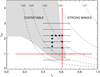 |
Fig. 2 Conducted simulations in rh, τdyn parameter space. Contours indicate the number of simulation particles in the 10λcr × 5λcr runs when identical particles are used (see Eq. (16)). Thick red lines indicate surveys illustrated in Figs. 5 and 7 in Mondino-Llermanos & Salo (2023), while black lines indicate range of other surveys made. Shaded region (from Fig. 10 in Mondino-Llermanos & Salo 2023) indicates the regime where overstability is obtained in simulations with identical particles with ϵn = 0.1. Circles stand for size distribution runs with W = Rmax/Rmin = 20, q = 3, with filled circles indicating overstable cases. In experiments with W = 20, the number of particles is ~7 times larger than indicated by the contours (see Appendix A). |
3 Illustrative examples of wakes and overstability
Before presenting results from systematic surveys over the parameter space, we illustrate in Fig. 3 examples of the expected photometric signatures in the presence of inclined self-gravity wakes and/or axisymmetric overstable oscillations. The upper-most row shows cartoons of how inclined wakes and axisymmetric structures would appear at different ring longitudes θ, counted from sub-observer direction. The self-gravity wake example (left frames of the figure) is selected to represent rather strong wakes obtained for rh = 0.8, corresponding to, say, a Saturnocentric distance of a = 123 000 km for an internal density of ρ = 450 kg m−3. The other example (right frames of the figure) with rh = 0.58 corresponds to the regime where weak self-gravity wakes are embedded among strong overstable oscillations (for example, ρ = 300 kg m−3 and a = 102 000 km). In both cases, identical particles are assumed with τdyn = 1 and ϵn = 0.1.
In the rh = 0.8 case, the individual wakes appear rather twisted, with a large spread in their instantaneous orientations. Nevertheless, the time-averaged autocorrelation function indicates a well defined pattern, corresponding to an average wake pitch angle ϕw = 20°, counted counter-clockwise from the direction of mean orbital velocity. Thus, when the simulation system is placed in the ring longitudes θ = 90° − ϕw = 70° or θ = 270° − ϕw = 250°, they are viewed along the average direction of wakes, as depicted in the ring cartoon. For low viewing elevations, the reflecting area is then minimised, due to optimal visibility of rarefied inter-wake regions. Similarly, on longitudes θ = 180° − ϕw = 160° and θ = 360° − ϕw = 340° the wakes are viewed more or less side-on, hiding the gaps and thus corresponding to maximum reflecting area and maximum expected brightness. The actual photometric modelling, shown in the two lowermost frames quantifies these expectations, indicating a broad minimum of I/F around ring longitude θmin = 250° (together with a similar minimum at θ = 70°). Likewise, τphot has a minimum for light rays passing through the system at the same longitudes.
For weaker self-gravity, rh = 0.58, the trailing self-gravity wakes are still visible in snapshots but are much less pronounced. Instead, the system is dominated by axisymmetric overstable oscillations. Compared to case of strong wakes, the density contrasts are much weaker, consistent with the smaller I/F variations with longitude. Photometric modelling indicates that the minimum I/F is attained at θ = 261° (and 81°), which would formally correspond to effective ϕw = 9°. However, the connection of brightness minimum to auto-correlation function is now less clear, since the latter is almost totally dominated by the regular axisymmetric pattern due to overstability. Rather, the effective pitch angle corresponds to the pitch angle of the weak wakes in the rarefied zones between the density crests of overstable oscillations: these wakes appear more tangential than the strong wakes in rh = 0.8 case. In the τphot profiles the signature of over-stability is clearer than in I/F, since even a small difference in the number of transmitted photons matters. The minimum τphot is likewise achieved closer to ansae than in the rh = 0.8 case, although the shift is smaller than for the longitude of minimum I/F. Also note the overall larger mean τphot compared to the strong wake case even if the τdyn are the same.
In the surveys of Sects. 4 and 5, the amplitude of I/F variations is measured with the full amplitude
 (19)
(19)
where Imax and Imin are the global maximum and minimum I/F over all ring longitudes. However, when comparing the models to French et al. (2007) HST observations in Sect. 7, the amplitude
 (20)
(20)
is used. This quantity was used in French et al. (2007) since typically only a partial ring patch around the minimum is accessible in observations. For example, in HST observations with B = 15° the maximum Aasym = 0.28 at the mid A ring (128 000 km), while the corresponding A40 = 0.17 (French et al. 2007). To quantify the variations in ring transparency we use a definition similar to Eq. (19),
 (21)
(21)
where Tmax and Tmin are the maximum and minimum fractions of photons, I/I0, transmitted through the ring along the viewing elevation B, related to τmin and τmax, respectively, via Eq. (3).
In most of the figures, we measure the ring longitude with ∆θ = θ − 90° or θ − 270°, the longitude with respect to ansa.Similarly, we define ∆θmin to be the longitude of minimum brightness (or minimum τphot) with respect to ring ansa. For the geometry in Fig. 3, ∆θmin ≈ −ϕw in the case of strong self-gravity wakes. However, in general the location of the minimum depends on observing geometry: for small phase angle HST observations French et al. (2007) found that the minimum of I/F falls halfway between the ring longitudes where the wakes are viewed or illuminated along their long axis, corresponding to
 (22)
(22)
where ∆λ⊙ is the longitude of Subsolar point with respect to Subobserver direction. The longitude of minimum I/F depends also on elevation angles, in HST observations shifting slightly closer to ansa for smaller viewing elevation. This can be interpreted in terms of the auto-correlation function, which becomes less inclined at the outer parts, which dominate more and more of the reflected light at low viewing angles (Salo et al. 2004; French et al. 2007).
In the current study, we limit to a fixed geometry B = B′ = 12°, ∆λ⊙ = 0° (except in Sect. 7.3 when comparing ring transmission as a function of elevation). Photometric comparisons with fixed geometry makes it easier to see what is the effect of varying the dynamical parameters.
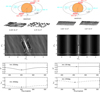 |
Fig. 3 Illustration of two simulations, representing strong (rh = 0.80; left) and intermediate strength of self-gravity (rh = 0.58; right). The former case leads to prominent wake structure, the latter to overstable oscillations with weak embedded wakes. The cartoon in the uppermost row illustrates how such systems would appear at different ring longitudes, when viewed from B = 12° elevation. Orbital motion is counter-clockwise in the figure. The next row shows the normalised density autocorrelation function from these experiments: in the left the shading, from white to black corresponds to 0.5 to 1.5 (contours mark 0.8, 0.9, 1.1, 1.4), while in the right the range 0.75 to 1.25 is shown (contours 0.8, 0.95, 1.1, 1.2). The white curve near the bottom of the frames is a radial cut of the autocorrelation at ∆y = 0. The last two rows display the modelled I/F and τphot versus ring longitude, for B = B′ = 12° and ∆λ⊙ = 0°. Symbols mark the minimum of modelled I/F and τphot. Both the autocorrelation plots and the photometric curves are averages over 40 snapshots; for each snapshot 105 photons were followed for 36 ring longitudes separated by 10°. |
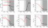 |
Fig. 4 Photometric quantities extracted from τdyn = 1, ϵn = 0.1 simulations, performed for various values of rh. The simulations marked with black symbols, for rh ≥ 0.61 are the same simulations as displayed in Fig. 7 of Mondino-Llermanos & Salo (2023), with the calculation size of 5λcr × 10λcr. The red symbols indicate simulations with rh < 0.61: to have a better statistics in photometric calculations, the simulated region does not scale with λcr but has a fixed size of 350 × 175 particle radii (this corresponds to 5λcr × 10λcr at rh = 0.61). The upper row shows quantities related to the azimuthal I/F profiles: the minimum and maximum brightness, the amplitude Aasym defined in Eq. (19) and ∆θmin, the longitude of I/F minima wrt to ansae. In the case of self-gravity wakes, their pitch angle ϕw = −∆θmin. In the middle upper panel, the dashed curve corresponds to Lambert-phase function with ϖ = 0.7; in other cases Callisto phase function with ϖ = 0.4 is assumed. The lower row displays similar quantities derived from the optical depth profiles. Light shading (rh = 0.5–0.6) indicates the regime where overstability emerges and grows in amplitude, while the dark shading marks the regime where wakes suppress overstability (rh > 0.65). |
4 Photometric survey: Identical particles
In this section, we highlight how the I/F and τphot azimuthal variations depend on the strength of self-gravity, measured with the rh parameter, as well as on the assumed elasticity and dynamical optical depth. Unless otherwise indicated, the dynamical simulation models use identical particles with τdyn = 1 and ϵn = 0.1.
4.1 Survey over rh
Figure 4 displays how various photometric quantities depend on the strength of self-gravity, measured with the rh parameter. The size of the calculation region is selected so that it covers at least 10 × 5 critical wavelengths, thus Lx and Ly increase in physical units proportional to rh3. However, for rh < 0.61 we have fixed the particle numbers and calculation region to that with rh = 0.61, in order to assure that there are enough particles (N ∼ 20 000) to give statistically accurate MC results. In the figure the black and red colours distinguish these parameter regimes; this is convenient because it also highlights the wake-dominated regime rh ≳ 0.6. On the other hand, overstable oscillations are present for 0.5 ≲ rh ≲ 0.65 (see Fig. 7 in Mondino-Llermanos & Salo 2023).
The upper row of Fig. 4 shows quantities related to I/F brightness profiles, while the lower row collects corresponding quantities for τphot profiles. In the case of weak self-gravity, rh ≲ 0.6, the ring brightness is nearly independent of the viewing longitude, but for rh ≳ 0.6 the asymmetry amplitude rises rapidly as self-gravity wakes get stronger, with a peak of Aasym ≈ 0.6 at rh ≈ 0.8. For still larger rh the amplitude slowly declines, which relates to increasing clumpiness of the wakes, so that their reflecting area is less dependent on viewing azimuth (Salo et al. 2004; French et al. 2007). For rh ∼ 1.1–1.2 the asymmetry would vanish as wakes collapse to gravitational aggregates. The overstable oscillations for rh = 0.5–0.6 have no clear effect in I/F or Aasym, but on the other hand, the overall τphot decreases in the overstable regime and Atrans grows, reaching a peak amplitude 0.8 at rh = 0.65, corresponding to τphot-range 0.7 – 1.0. We note that the peak Atrans has no specific significance: the minimum τphot, determined by the prominence of gaps between the wakes, is still decreasing with rh, reaching τphot ∼ 0.15 for rh ≳ 0.7.
The two curves in the middle upper panel illustrate the small effect the choice of the phase function has on brightness asymmetry: the dashed curve corresponds to Lambert-phase function which leads to a larger contribution from multiple scattering and thus to slightly increased brightness contrast between dense wakes and rarefied inter-wake regions. The effect is so small that we shall not explore it further in relation to other quantities (for further examples, see French et al. 2007).
What is quite interesting is the strong trend in the longitude of I /F minimum with rh. In the wake dominated region the inferred pitch angle (ϕw = −∆θmin) increases from about ϕw = 15° to 20° when rh increases from 0.6 to 0.9. In the overstable regime (rh = 0.5–0.6) ϕw is close to zero, as expected when axisymmetric oscillations become important. However, what is quite unexpected is the large positive values of ∆θmin in the regime where no overstability nor significant wakes are present: the minimum I/F occurs even 40° after the ansa for rh ≲ 0.3. Although the amplitude of these ‘anomalous’ I/F variations is very small (∼1%) they indicate the persistent presence of weak leading density features in the particle field. Similar leading signal is seen in τphot minimum longitude, with amplitude Atrans = 0.65 at rh → 0. In spite of the high relative amplitude, the effect is quite subtle: the minimum τphot ≈ 1.4 for rh → 0 corresponds to a maximum transmission of only about 0.1% for B = 12°. We analyse this unexpected small rh behaviour in more detail in the next subsection.
4.2 ‘Anomalous’ asymmetry at rh → 0
In principle, such ‘anomalous’ τphot variations seen in nongravitating and weakly gravitating simulations could be an artifact, resulting from a small number of ‘leaked’ photons through uniformly distributed particle fields. For instance, this could happen due to inaccuracies in the treatment of periodic boundaries or in the search of photon path intersections with particles. However, several tests with a varied calculation region size and aspect ratio all gave consistent results. Also, tracking the locations of photon paths passing through the system indicated no relation to periodic boundaries. Similarly, tests with truly uniform particle fields (random placement except with no overlaps between particles or image particles) showed no trace of such behaviour.
Figure 5 shows the I/F and τphot profiles for weakly gravitating systems with rh = 0–0.61. At rh close to zero, there is a maximum in I/F and τphot at ∆θ ∼ −40°, which is gradually superseded by the minimum associated with overstability and/or wakes. This superposition of variations creates the appearance of a smoothly varying minimum longitude, shifting from ∆θmin = 40° to ∆θmin = −20° as rh increases from zero to 0.61. A similar gradual change is seen in the τphot profiles.
We conclude that the simulated τphot and I/F variation is real, resulting from a low-level leading polarisation of the particle field. Indeed, in the case of small velocity dispersion the distribution of impact directions is not fully isotropic, but because of the shear the impacts concentrate on the leading quadrants of the particles. After impact the particles separate but with a reduced relative speed, which causes a slight over-density on the leading quadrants, making the system’s reflectance weakly dependent on the orientation. Moreover, the significantly non-zero τphot amplitude suggests that there are preferential orientations for photons to pass through the layer. The lower frames of Fig. 5 shows examples of auto-correlation functions, both for the particle positions (similar to those in Fig. 3 except now concentrating on the very central part), and for the transparency of the system (as seen from perpendicular direction). A non-gravitating rh = 0 case is chosen, to fully eliminate any disturbances caused by weak wake-structures. In the density autocorrelation function (left) we see clearly the density enhancements related to impacting particles in temporary contact: the red circles have radii of 1R, 2R and 4R. The arrow marks the viewing direction corresponding to minimum of I/F azimuthal profiles: the density enhancements, in particular those at ∼4R, are most elongated along this direction. Apparently the low B cross-section in this direction is sufficiently reduced to yield the slight 0.5% drop in brightness. In the lower right panel, the autocorrelation function of transmission is shown for B = 90°. Again, the arrow marks the direction of minimum of τphot.
The central peak of the transmission autocorrelation function is clearly elongated in the same direction.
Figure 6 illustrates the smooth change in the density autocorrelation function taking place when rh increases and the system starts to develop overstabilities and wakes. The leading-quadrant condensations of particles, similar to those depicted in Fig. 5 for rh = 0 are always present, and in fact get stronger with stronger gravity as would be expected. However, they are overwhelmed by the global structures, first due to overstability (middle frame for rh = 0.56) and eventually by growing gravity wakes (right frame with rh = 0.61).
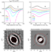 |
Fig. 5 ‘Anomalous’ asymmetry at weakly gravitating systems. Upper row: I/F and τphot profiles in simulations with rh = 0–0.61. Error bars indicate the error of the mean, calculated from the RMS values over 20 snapshots. Arrows mark the location of the minimum I/F and τphot in non-gravitating rh = 0 run. Lower row: autocorrelation functions of density and transmission for rh = 0. Only the central parts are show: circles correspond to 1, 2, 4 particle radii. The density autocorrelation was constructed from number density of particle centres. The transmission autocorrelation was calculated from a binary table constructed by illuminating the particle field vertically with 25 ⋅ 106 photons, and assigning values 0 and 1 for locations where photons were intersected/not intersected by any particle, respectively (resolution of the grid was 0.3 particle radii). In both cases a normalised autocorrelation is displayed, the grey scale extending from 0.9 (black) to 1.1 (white). Arrows indicate the viewing directions corresponding to the minimum of I/F and τphot. |
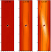 |
Fig. 6 Density autocorrelation functions for rh = 0.40, 0.56, and 0.61. The central 30 × 120 particle radii regions are shown, while λcr/R = 9.7, 29.4, and 34.2, respectively. Contours mark overdensities of 1.1, 1.2, and 1.3; for clarity contours are not shown for the central region. In all runs τdyn = 1.0 and ϵn = 0.1. |
4.3 Effect of particles’ elasticity law
The above survey of rh was performed with ϵn = 0.1. In the case of such dissipative impacts, the steady-state velocity dispersion maintained by impacts is small, cr ∼ RΩ, making the system susceptible to both formation of self-gravity wakes and viscous overstable oscillations (according to Eq. (12), Q ≲ 2 for rh ≳ 0.3 when τdyn = 1). Figure 7 extends the models of Fig. 4 to ϵn = 0.50 and to velocity-dependent ϵn with vc/vB = 5, which yields roughly 1.5 and 3.5 times larger steady-state velocity dispersions in the non-gravitating case compared to ϵn = 0.1. Clearly, for more elastic particles the rise in Aasym amplitudes is shifted towards larger rh values. For a fixed distance, a, this means that a larger internal density would yield a similar Aasym. For example, for ϵn = 0.50 the small ∆rh ≈ 0.03 shift in Aasym vs rh curve would be compensated by about 10% increase in ρ, while for vc/vB = 5 a nearly doubled ρ would be needed.
In the case of constant ϵn = 0.5 the rh region where overstability develops is fairly similar to that of ϵn = 0.1, except that the amplitude of overstability is weaker. A very similar behaviour is obtained with velocity-dependent elasticity, using vc/vB = 1. In contrast, for vc/vB = 5 there is no sign of overstability for any rh, consistent with the fact that FF(0) never exceeds about 0.22 (maximum attained at rh ≈ 0.6). For comparison, at rh = 0.61, FF(0) = 0.40 for ϵn = 0.1 and FF(0) = 0.37 for ϵn = 0.5. On the other hand, even with vc /vB = 5 self-gravity wakes are present, although a larger rh is needed before they grow to sufficient strength to cause significant asymmetry.
We also carried out simulations with vc/vB = 20 (for clarity not shown in the figure), implying a dynamically hot steadystate with no self-gravity wakes (in this case the steady-state Q ≳ 5). When rh is small, such systems remain uniform, but for rh ≳ 0.7 they exhibit viscous instability; that is, collisions lead to the amplification of random density fluctuations. This follows from the dominant role of local viscosity, and the fact that due to high-steady state velocity dispersion, the dynamic viscosity is now a decreasing function of density (see Salo et al. 2018). Interestingly, stronger self-gravity enhances this tendency for viscous instability and is able to flip a marginally stable system at small rh to an unstable one when rh is sufficiently large. The end result of viscous instability is a saturation state where the system is separated into dynamically cool dense ringlets and dynamically hot rarefied zones, with the dense regions exhibiting embedded self-gravity wake structures (see Salo & Schmidt 2010). Wakes appear, as the growth of density and the reduction of velocity dispersion inside the ringlets has reduced Q sufficiently for wakes to form. However, such a combination of viscous instability and embedded wakes is probably a curiosity, unlikely to have observational counterparts as such an elasticity law with vc/vB >>1 would not allow for viscous overstability to take place at any distance.
Besides comparing elasticity models, Fig. 7 collects photometric results for ‘hybrid’ simulation models explored in Mondino-Llermanos & Salo (2023). In such models the vertical and planar self-gravity are separated: planar components of gravity are calculated self-consistently whereas the vertical field is treated as in Wisdom & Tremaine (1988), assuming an enhanced vertical frequency, Ωz/Ω > 1. Such a separation of vertical forces gives a handle to the flattening of the system, while keeping the self-consistent calculation of planar gravity. With the values adopted in Fig. 7, the system is strongly flattened, with FF(0) ∼ 0.50–0.55 for rh ≲ 0.75 when Ωz/Ω = 4.4. Accordingly, such simulations develop overstable oscillations even in the absence of planar self-gravity. For a given rh this extra vertical flattening weakens the self-gravity wakes, as the planar forces exerted by strongly flattened wakes are reduced compared to what they would be if the wakes had a typical less flattened crosssections (see Fig. 21 in Sect. 7). As a consequence, the system behaves as having a smaller effective rh. Because of this, the regime of strong wakes is shifted to rh ≳ 0.75 when Ωz/Ω = 4.4. For Ωz/Ω = 7.5 the shift in rh is even more pronounced. Due to reduced planar gravity, overstable oscillations can take place for larger values of rh before being suppressed by strong wakes.
In Mondino-Llermanos & Salo (2023), we argue that at least to some degree this ‘hybrid’ method with Ωz/Ω > 1 mimics the inclusion of particle sticking forces such as included in simulations of Ballouz et al. (2017), which likewise allowed the overstability to survive in simulations with increased rh. According to Fig. 7, there is a substantial shift in asymmetry amplitude: the peak Aasym is achieved at rh ∼ 1 when Ωz /Ω = 4.4, compared to rh ∼ 0.75 in the self-consistent case with the same ϵn = 0.1 and τdyn = 1.0. Beyond rh ∼ 0.8 the overstability is suppressed in the hybrid simulations: this corresponds to the same νgrav /νnl ≳ 0.4 limit that is reached with rh > 0.65 in the standard ϵn = 0.1 simulations (see Appendix B).
Simulations of Sect. 4.1 indicated pronounced anomalous asymmetry for rh → 0 in case ϵn = 0.1. For less dissipative and thus dynamically hotter and vertically more extended systems, one would expect reduced variations. Figure 8 confirms this expectation, comparing the strength of anomalous variations in the case in which the system’s geometric thickness is increased via assuming more elastic particles. Again, we focus on rh = 0 to eliminate the effect of any overstabilities and/or wakes. The polarisation was relatively weak even at ϵn = 0.1 case, and becomes rapidly weaker when larger ϵn or a velocity dependent ϵn(vn) are assumed. When using ϵn = 0.5 instead of ϵn = 0.1, the τphot amplitude is reduced from 0.2 to 0.1. In this case the system effectively translates from a double layer (H/R ∼ 4) to a three-layer system (H/R ∼ 6). The other two profiles shown in the figures are from runs with velocity dependent ϵn, in which case the steady-state H ∝ vc/Ω for vc >> vB. For example with vc/vB = 20 the system is a multilayer with H/R ∼ 30, and the anomalous amplitude is fully insignificant. The figure also highlights how τphot /τdyn increases significantly from unity when the geometric thickness of the system approaches the size of particles (Salo & Karjalainen 2003).
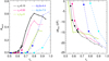 |
Fig. 7 Photometric quantities extracted from τdyn = 1 simulations, using different elasticity laws, ϵn = 0.1, 0.5, and Bridges-formula with vc /vB = 5. Additionally, dashed line indicates results from simulations with a ‘hybrid’-method, with Ωz/Ω = 4.4 and 7.5, both using ϵn = 0.1. Filled circles denote runs developing overstability. |
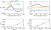 |
Fig. 8 Dependence of ‘anomalous’ asymmetry on ring thickness. Upper row: I/F and τphot profiles in non-gravitating rh = 0 runs, using different elasticity models. In each case τdyn = 1.0. The numbers next to τphot profiles indicate the H/R ratio, where |

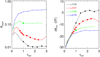 |
Fig. 9 Asymmetry properties as a function of dynamical optical depth, for the transition region between overstability/wakes, rh = 0.58–0.70. The large solid symbols indicate simulations that develop prominent overstable oscillations, while wake structure is present in all cases. |
4.4 Effect of τdyn
In the above simulations with τdyn = 1, the transition from overstable to wake-dominated systems was very smooth, characterised by a gradual increase in the asymmetry amplitude and a similarly gradual shift in the minimum longitude as rh increased. We also made simulations where τdyn was varied in simulations with a fixed rh, concentrating on the rh region where the transition from overstable oscillations to self-gravity wakes takes place. According to Fig. 10 in Mondino-Llermanos & Salo (2023), in non-gravitating case overstability sets in at τdyn ≳ 2 for rh ≲ 0.2 when identical particles with ϵn = 0.1 are simulated (see also our Fig. 2). For stronger self-gravity the threshold value gradually decreases reaching τdyn = 0.7–0.8 for rh = 0.5–0.65. For still larger rh the strong wakes suppress completely the formation of overstable oscillations. As mentioned earlier, rh ∼ 0.6 to 0.65 is an interesting regime where overstability first appears at intermediate τdyn but is then killed by wakes for larger τdyn.
The results for photometric calculations are collected to Fig. 9, for rh = 0.58 to 0.70. In the figure, filled circles indicate simulations leading to overstable oscillations. Self-gravity wakes are clearly present in all simulations, including the τdyn = 0.1 cases. Not surprisingly, in the case of strong wakes the minimum I/F is substantially reduced at all τdyn’s, consistent with the larger Aasym. Also, for τdyn ≳ 1, the ring brightness I/F and Aasym are practically independent of τdyn. Interestingly, in the case of weak self-gravity wakes (rh = 0.58 and 0.61), Aasym drops with τdyn. This reduction of amplitude manifests a photometric saturation effect for a nearly uniform particle layer. In contrast, in the case of strong gravity the effect of rarefied gaps becomes dominant with increasing τdyn.
For small τdyn ≲ 1, the effective pitch angle (ϕw = −∆θmin) is practically independent of rh, approaching ϕw ∼ 30° when τdyn = 0.1. This corresponds to direction of the centre-most part of wake autocorrelation function (see e.g. Fig. 5 in Salo et al. 2004). For τdyn > 1, ϕw varies in the range 0° – 20°, depending whether the system is dominated by overstable oscillations or by wakes. However, the transition between these cases is quite smooth. Also, the suppression of overstability and transition to wake-dominated system for rh = 0.61 when τdyn > 2–2.5 causes just a small upward turn in Aasym curve and a similarly modest increase in ϕw.
The parameter region of Fig. 9 was deliberately chosen to avoid the anomalous asymmetry, which partially hides the effect of wakes and overstability in the range rh = 0.4–0.5. A few additional experiments with rh = 0 showed that the amplitude of anomalous I/F asymmetry stays in a similar Aasym ≈ 0.01 level for τdyn = 2 as for τdyn = 1 in Fig. 5. For τdyn = 0.5 and 0.25, the amplitude is even slightly higher, Aasym ∼ 0.02 and 0.03, respectively. In τphot the anomalous asymmetry drops from Atrans = 0.6 at τdyn = 1 to Atrans = 0.05 at τdyn = 0.25.
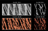 |
Fig. 10 Examples of how size distribution affects the ring structure/asymmetry. In the left 10λcr × 4λcr simulations with rh = 0.61, both with identical particles (W = 1) and with size distribution (W = 20). In the right, comparison to rh = 0.80 simulations with W = 1 and W = 20; the calculation size is 4λcr × 4λcr. Other parameters are τdyn = 1.0, ϵn = 0.1. |
5 Power-law size distribution
So far, all the presented models have assumed identical particles. Even in the absence of self-gravity wakes or overstable oscillation, the photometric properties of particle fields are sensitive to the width of the particle size distribution, W = Rmax /Rmin. Namely, the contribution to the amplitude and angular extent of the opposition brightness peak, arising from reduced mutual shadowing between particles when α → 0°, depends on W (Salo & French 2010). To eliminate this dependence we perform our size distribution models for exact opposition α = 0°, similarly to the identical particle models of the previous section, and thus avoid any effects caused by different magnitude of opposition brightening.
5.1 Competing effects of size distribution
When wakes or overstabilities are present, there are competing dynamical effects related to size distribution. Firstly, the smaller particles achieve a larger steady-state velocity dispersion than the large particles, which tends to reduce the density contrast of wakes and rarefied inter-wake regions among the population of small particles (Salo et al. 2004; French et al. 2007). The increased vertical thickness associated with increased velocity dispersion is also most likely the factor that shifts the onset of overstability to larger τdyn when size distribution is included, compared to identical particles. This stems from the implied reduced space density of particles, which needs to be compensated for by larger τdyn before overstability sets in. For example, for rh = 0.61 the central plane filling factor FF(0) at τdyn = 1 decreases from 0.40 to 0.32 when W changes from 1 to 20, the reduction of which is enough to convert an overstable system to a stable system (see Fig. 2). However, for τdyn = 1.4, W = 20 the filling factor FF(0) rises to about 0.39 and the system becomes again overstable.
Secondly, inclusion of size distribution promotes the formation of gravity-bound particle pairs and aggregates, as the effective rh for the small-large particle interaction is larger than for pairs of identical particles (see Eq. (11)). Also the maximum filling factor inside self-gravity wakes is increased, since small particles can fit into the voids between large particles. For example, self-gravity wakes start to collapse to gravitational aggregates at smaller distance with size distribution compared to simulations with identical particles. In simulations of Karjalainen & Salo (2004) the use of W = 10 reduced the rh leading to gravitational accretion from about rh = 1.2 to rh = 1.1 when Bridges-elasticity law was assumed.
The relative importance of these competing dynamical effects depends on the rh-regime: in the τdyn = 0.5 A-ring models with strong wakes studied in French et al. (2007), the reduced density contrast between wakes and inter-wake regions dominated and thus the inclusion of size distribution led to smaller asymmetry amplitude. However, our current extended survey with a larger range of τdyn indicates that the opposite is possible in the case of weaker gravity: the extra boost from larger effective rh and the larger maximum filling factor inside wakes for W>>1 can lead to substantial increase in the strength of wakes and thus to larger Aasym. It can also turn an overstable system to a wake-dominated system.
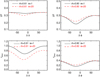 |
Fig. 11 I/F and τphot versus ring longitude, for weak (rh = 0.61; left frames) and strong self-gravity (rh = 0.8; right frames). Colours indicate profiles for identical particles (W = 1) and for W = 20 size distribution. |
5.2 Effects of size distribution in weak and strong gravity regimes
The competing effects of the size distribution are illustrated in Figs. 10 and 11. In the former figure the snapshots in the right column show a simulation with strong wakes (rh = 0.80), resembling the runs used in French et al. (2007) to model the maximum A-ring asymmetry. Using W = 20 instead W = 1 reduces Aasym for τdyn = 1 by nearly a factor of two, from 0.63 to 0.35. Additional experiments with rh = 0.85, τdyn = 0.5 (Appendix C; these are even closer to models in French et al. 2007) indicated even stronger reduction, from Aasym = 0.48 to 0.23. The I/F and τphot profiles in Fig. 11 (right frames) confirm that the reduced amplitude stems from the more shallow minimum in the case of W = 20, reflecting the more uniform distribution of smaller particles, which leads to increased optical depth of the gaps. Another factor is the more clumpy and twisted morphology of wakes.
On the other hand, the snapshots in the left frames of Fig. 10 correspond to weaker gravity (rh = 0.61), leading to overstable oscillations and weak embedded wakes when W = 1. However, when W = 20, the system develops strong wakes, with no trace of overstable oscillations. The asymmetry amplitude is over three-fold compared to W = 1 simulations (0.14 instead of 0.04). In the I/F profiles (shown in Fig. 11), the depth of the minimum has become substantially deeper due to appearance of inter-wake gaps. The increased transparency of the system also reflects in the overall reduction of τphot.
Figure 12 (upper frames), explores systematically the effect of the size distribution width on Aasym and ∆θmin, for the same rh = 0.61 and rh = 0.80 values as in the previous figures. Besides the ϵn = 0.1 simulations displayed in the figure, also simulations with ϵn = 0.5 were conducted, as more elastic impacts can lead to larger differences between small and large particle velocity dispersions (see Fig. 19 in Salo et al. 2018). Nevertheless, except for a generally smaller Aasym for ϵn = 0.5 the trends with W are similar: for strong wakes larger W suppresses Aasym effectively while the opposite takes place for weaker gravity. Clearly, the drop in Aasym for rh = 0.80 continues even beyond the distribution with W = 20 illustrated in Fig 10. See Appendix C for additional examples, displaying snapshots for systems with different W up to 100.
For weaker self-gravity, the growth of Aasym with W is more modest, with no essential difference between W = 10 and W = 100. This is understandable, as there is a limit of how much the effective packing density can increase in the presence of small particles: even if the packing density would rise from 0.704 (identical spheres) to unity, this only corresponds to 10% increase in effective rh. Additional simulations indicate that these competing effects on Aasym, due to increased velocity dispersion and due to a larger effective filling factor in case W >>1, more or less cancel each other at rh ≈ 0.7 (see the next section).
Also shown in Fig. 12 (upper right frame) is the effect of W on the location of the brightness minimum. In all cases, there is a systematic increase on the effective pitch angle when W increases, reaching values ϕw = −∆θmin = 20° – 25°. However, the reason for this behaviour is somewhat different in weak and strong rh regimes. For rh = 0.61 the increased ϕw is related to the distinct transition from axisymmetric overstable oscillations to a wake-dominated system (see Fig. 10). In contrast, for rh = 0.80 the wake structures from W = 1 and W = 20 simulations appear superficially quite similar. Nevertheless, the wakes are shorter and more patchy when W increases, increasing the effective ϕw. This clumpiness probably stems from the large relative size of the largest particles compared to the separation between wakes, which is of the order of λcr: for W = 20, Rmax/λcr ∼ 0.1. In this sense extended size distribution runs resemble simulations with smaller τdyn < 1, which also have a large R/λcr ratio. According to Fig. 9, τdyn < 1 leads to increased ϕw. The increased patchiness and its connection to ϕw is further illustrated by the examples in Appendix C; see in particular the τdyn = 0.5, rh = 0.85 example where ϕw reaches even 35° with W = 100.
6 Asymmetry amplitude and gravitational viscosity
The surveys of previous sections have explored the azimuthal brightness and opacity variations arising in the presence of self-gravity wakes, and to a lesser extent due to overstable oscillations. From the same dynamical simulations, also various contributions to viscosity were tabulated. In particular, the measured νɡrav provides a quantitative gauge for the strength of wakes. In the lower frames of Fig. 12, total viscosities and various contributions to viscosity are depicted against the width of size distribution, for weak and strong self-gravity cases. At rh = 0.61, nonlocal contribution dominates viscosity, comprising two-thirds of the total for identical particles and nearly half for W = 100. As W increases, the νɡrav contribution also rises, reflecting the increased prominence of wake structures, as evidenced by the larger Aasym. However, the substantial decline of Aasym for rh = 0.80 with increasing W does not imply that the wakes disappear: in this case νɡrav is about the same for all W. This supports our view that the wakes remain dynamically strong but become increasingly shrouded by more evenly distributed population of smaller particles. In cases of strong wakes, the contribution from νnl is negligible irrespective of W. For local viscosity, the relation νl ∼ νɡrav holds well for strong wakes, though the actual value of νɡrav can be larger than implied by Eq. (14).
The measured viscosities of the experiments of Sect. 4.3 at different rh are compared in Fig. 13. Also shown are asymmetry amplitudes, but now measured with A40, as this is the quantity that will be compared with observations in the next section. Both identical and extended size distribution simulations with W = 20 are shown, as well as hybrid simulation models with Ωz/Ω = 4.4 and 7.5. Additional models (with varied τdyn and with ϵn = 0.5) are shown in Appendix B.
Comparison of A40 versus rh (left frames) shows that for W = 20 the asymmetry amplitude rises to an 1% level already at rh ≈ 0.5, compared to identical particles where this takes place at rh ≈ 0.6. The amplitude curves for W = 1 and W = 20 cross at rh ∼ 0.7, beyond which the size distribution leads to a smaller A40 than identical particles. This behaviour is consistent with that illustrated in Figs. 10 and 12. These trends in A40 are reflected on the νɡrav vs rh curves (middle frame), in the sense that the rise of νɡrav is similarly delayed with W = 1. However, for rh ≳ 0.75, νɡrav is no longer affected by the width of the size distribution.
For the hybrid Ωz/Ω = 4.4 and 7.5 simulations, much larger rh are required before the asymmetry amplitude becomes significant, compared to simulations with self-consistent vertical field. These trends in A40 are again reflected on the νɡrav vs rh curves. It should be noted, however, that the total viscosity (right frame) for a given rh ≲ 0.7 is largest for the hybrid simulations, due to a strongly enhanced non-local contribution (see also Appendix B).
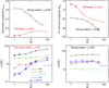 |
Fig. 12 Effect of size distribution on azimuthal asymmetry and ring viscosity. Upper frames: Aasym and ∆θmin in the case of strong (rh = 0.80) and weak (rh = 0.61) self-gravity. The width of size distribution is varied, while keeping τdyn and Σ fixed by a suitable choice of Rmin and Rmax (see Appendix A). Filled circles indicate overstable simulations. Lower frames: total viscosities and various contributions to viscosity as a function of W, for weak (left) and strong (right) self-gravity. Box symbols denote νgrav calculated from density autocorrelation function (see Appendix B). The viscosities are normalised with ΩRo2 where Ro in the case of size distribution denotes the identical particle size, R, that yields the same τdyn and Σ. Dashed lines in the right axis indicate the νɡrav from Daisaka et al. (2001) viscosity formula, Eq. (14). In all simulations τdyn = 1, ϵn = 0.1. |
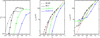 |
Fig. 13 Comparison A40 and νɡrav as a function of rh, collecting different simulation series as indicated by the labels (unless otherwise indicated, τdyn = 1, ϵn = 0.1, W = 1). In the middle frame, νɡrav is shown, while in the right, νtot is. The dash-dotted red curve in the middle frame shows the νɡrav calculated from Eq. (14), while in the right it indicates 2νɡrav. |
7 Applications to Saturn’s rings
In the above sections, we have made a systematic exploration of the influence of various dynamical quantities on the expected photometric properties of the simulation system, both in overstability-dominated and self-gravity wake- dominated regimes. In this section our goal is to constrain the range of plausible models via comparisons to HST observations of asymmetry amplitude. Additionally, we compare to the Cassini measurements of ring transparency and estimate the kinematic viscosity in the B and A rings. Finally, a toy-model is presented for the decline of asymmetry amplitude in the outermost A ring due to impact-released debris.
An important constraint for the modelling is provided by the range of ring locations where evidence of overstable oscillations have been detected. In Cassini RSS occultations (Thomson et al. 2007), clear periodic radial density variations were detected for the inner A ring at a = 123 100–123 400 km and a = 123 600– 124 600 km, manifesting as symmetric diffraction side-bands around the direct signal. Wavelengths inferred from the frequency offsets were ∼160 and ∼220 metres, respectively, with ∼0° cant angle. These findings were confirmed by Hedman et al. (2014) high radial resolution VIMS occultation of the star γ Cru- cis covering the region 124 000–125 000 km, showing also that there are systematic variations in the strength and wavelength of the pattern, though these were not directly connected to local optical depth. However, the smallest τ ∼ 0.8 where overstability was detected is in agreement with dynamical experiments (see Fig. 11 in Hedman et al. 2014). The VIMS measurements also confirmed that the opacity variations remain azimuthally coherent at least for 3000 km. In the B ring, Thomson et al. (2007) detected similar periodic signals in three regions, at a = 92 100–92 600 km, 99 000–104 500 km and in a more muted form between 110 000–115 000 km, with inferred wavelengths of 115, 150, and 250 metres, respectively. In the regions were signal was detected the typical τ ∼ 1–1.5. The high radial resolution UVIS occultation of α Leonis (Colwell et al. 2007) confirmed the existence of almost perfectly azimuthal variations at a = 114 500 km. Most recently, Jerousek et al. (2024) carried out autocorrelation analysis of UVIS occultations, confirming the presence of overstabilities in the above-mentioned B ring regions. Also, their analysis of the inner A ring confirmed the simultaneous existence of wakes and overstabilities (see their Fig. 26a for a = 123 220 km).
7.1 Comparison to French et al. (2007) HST observations
French et al. (2007) made an exhaustive analysis of azimuthal asymmetry based on HST UBVRI imaging covering a complete Saturn season, with B ∼ B′ = 4°–27° and −7° < ∆λ⊙ < 7°. This study also contained a detailed comparison to photometric models calculated from dynamical models for self-gravity wakes. Although at that time the range of parameters in dynamical simulations was rather limited, many observed trends were extremely well accounted for. These included the dependence of the A-ring asymmetry amplitude on the elevation angle, the dependence of θmin on ∆λ⊙ (Eq. (22)), and the lack of a significant dependence of asymmetry on the wavelength, consistent with ring reflection being dominated by singly scattered flux. The HST observations provided evidence of asymmetry also in the inner B ring, quite similar in shape and location to the peak in the mid A ring, except with an amplitude about a factor of five smaller. What remained problematic was the rapid rise in the asymmetry amplitude from the inner to mid A ring, peaking at around a = 129 000 km, and the similarly rapid drop in amplitude beyond that distance. Also, the models made with identical particles yielded a very good match with the location of minimum I/F at the peak of asymmetry (∆θmin ∼ −21°), whereas the agreement with size distribution models was poor as they predicted ∆θmin ∼ −25°. These are factors we re-address with our new models covering a larger range of rh, τdyn, ϵn and a more extended size-distribution.
The main emphasis of the models in French et al. (2007) was modelling the maximum asymmetry in the mid A ring. Using models with τdyn = 0.5 and Bridges elasticity it was concluded that the best overall match is attained with internal density ρ ≈ 450 kg m−3. For this choice the models with identical particles matched also well the shape of I/F profiles at different elevations. The blue curves in Fig. 14 (upper frame) correspond to a model similar to that adopted in French et al. (2007), using three different assumed values of ρ for converting rh to distance a. The shading in the background shows the observed HST asymmetry amplitude. The choice of ρ ≈ 450 kg m−3 (highlighted with thick blue line) is qualitatively consistent with the maximum asymmetry amplitude in the A-ring region, also yielding a reasonable overall match with the inner B-ring asymmetry. In particular, a substantially larger ρ closer to solid ice density (900 kg m−3) would shift the asymmetry maximum to the B-ring region.
In the current study we prefer higher τdyn and more inelastic particles, since this is the combination that allows for viscous overstability to occur throughout the B ring and in the innermost A ring. The red curves in 14 (upper frame) corresponds to the identical particle model with τdyn = 1, ϵn = 0.1. In this case, the internal density roughly matching the A-ring asymmetry maximum is substantially smaller, about 250 kg m−3 (thick red line). For the moment, we ignore the fact that the model implies continuous rise of asymmetry amplitude well beyond the A-ring region (see Sect. 7.7).
To separate the effects of different τdyn and ϵn, the lower frame of Fig. 14 shows τdyn = 0.5 and 1.0 both with ϵn = 0.1 and ϵn = 0.5, the latter elasticity model giving practically identical results compared to vc /vB = 1 model used in French et al. (2007). Here the models are shown as a function of rh while the distances of HST observations have been converted to rh assuming ρ = 250 kg m−3. According to the figure, both the increase in τdyn and reducing ϵn increases the slope of the amplitude in the A-ring region. In fact, with our current standard parameter values (τdyn = 1, ϵn = 0.1) the rise of amplitude at the inner A-ring region is nearly as steep as observed. However, with the same model the inner B-ring asymmetry is absent: as we shall soon show that this defect can be alleviated by taking into account the particle size distribution, which according to Sect. 5 boosts asymmetry in the weak gravity regime.
A simultaneous comparison to HST asymmetry amplitude A40 and minimum longitude ∆θmin is done in Fig. 15. The curves show quantities from photometric models for different τdyn, both for identical particles (upper row) and for W = 20 size distribution simulations (lower row). Internal density ρ = 250 kg m−3 is assumed for converting the radial distances of HST observations to rh values. Also shown are the τPPS profiles from Voyager PPS stellar occultation experiment, compared to τphot in models with B = 28.7°, θ = 107°. The arrows in the ∆θmin frame mark regions where overstability is seen in UVIS, RSS, and VIMS observations (Colwell et al. 2006, 2007; Thomson et al. 2007; Hedman et al. 2014; Jerousek et al. 2024). With the chosen ρ the outermost distance where overstability has been observed, a ≈ 124, 000 km, corresponds to rh ≈ 0.65, a bit high but still marginally consistent with the largest rh allowing overstability to develop in ϵn = 0.1, W = 1 simulations (see Fig. 2). Similarly, the inner edge of the B ring corresponds to rh ≈ 0.5, consistent with the presence of overstability.
In the case of the inner and mid A-ring region, the W = 1 runs with τdyn ≳ 1 yield steeper slopes for the rise of A40 than the τdyn = 0.5 curve, though the slope of A40 vs rh does not increase much for τdyn ≳ 1–1.5. Increasing τdyn moves the minimum closer to ansa, but the maximal effect is similarly reached already for τdyn ∼ 1.5. For τdyn > 1, ∆θmin is in range −15° to −18°, deviating clearly from observations, which indicate ∆θmin ≈ −21° at a = 129 000 km. Thus, even if the steep rise of A40 is more or less satisfactorily accounted for by higher τdyn ≳ 1, none of these single-sized particle models is truly satisfactory.
On the other hand, a better match for ∆θmin is obtained by taking into account a particle size distribution (see the τdyn = 1, W = 20 model in Fig. 15, lower row). The same model also agrees reasonably well with the mid A-ring values of A40 and τpps. A drawback of the W = 20 model, compared to single-sized models with τdyn ≥ 1, is the fairly shallow slope of A40 with distance, similar to that in the case of lower τdyn = 0.5, W = 1. Additionally, to obtain overstability with such a size distribution model, a somewhat larger τdyn ≳ 1.5 would be needed (see Fig. 2). Nevertheless, this W = 20, τdyn = 1, ϵn = 0.1 model gives a quite good overall match for the observed asymmetry in the mid A ring, including the τpps profile shown in the rightmost frame.
Continuation of the identical particle models to the B-ring region accounts well the range of τpps measurements. However, none of the W = 1 models with τdyn ≳ 1 is able to account for the inner B-ring asymmetry. Taking into account the size distribution helps, as we are now in the weak self-gravity regime where the asymmetry gets stronger with increasing W. Concentrating on the regions within the ranges a = 95 000–99 000 km and a = 101 000–104 000 km, all three quantities (A40, ∆θmin, and τpps) are simultaneously well matched for W = 20 models with τdyn = 0.75 and τdyn = 2.2, respectively. Extrapolating such models to τdyn = 3–4 would most likely fit well also the third B ring region at a = 110 000–115 000 km having a nonzero A40. The other parts of the B ring are clearly too opaque to give observable asymmetry amplitude.
In summary, the current self-gravitating simulation models indicate a relatively good match to the A and B ring asymmetry amplitude and minimum longitude in HST observations. However, this is achieved only when assuming quite a low internal density of particles. In the previous sections we showed that the inclusion of an extra vertical force can shift the growth of self-gravity wakes to larger r′h s. Consequently, it is possible, at least in principle, to match the same radial trends of asymmetry amplitude with particles having larger ρ, by inclusion of such hybrid treatment. We shall return to this when comparing in Sect. 7.5 the viscosities of models to observations.
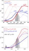 |
Fig. 14 Comparison of asymmetry amplitude A40 in simulations with different dynamical parameters. Upper frame: Blue curves assume to τdyn = 0.5 and velocity-dependent ϵn with vc = vB, as in models of French et al. (2007), while red curves assume τdyn = 1, ϵn = 0.1. Different internal densities ρ = 650, 450, and 250 kg m−3 are compared. Lower frame; comparison of the τdyn = 1.0 and τdyn = 0.5 simulations for ϵn = 0.1 and ϵn = 0.5; the latter elasticity law gives practically identical results to using velocity-dependent ϵn with vc = vB. The models correspond to B = B′= 12° and the HST values are weighted averages of 10° and 15° observations (see Fig. 20 in French et al. 2007). |
7.2 Trends between photometric quantities
Besides trying to match the trends of various observed quantities as a function of distance, which is very sensitive to the assumed internal density, it is also of interest to look at their relations with each other, both in observations and models. Figure 16, upper frame, compares the A40 amplitude with τpps. The B and A ring measurements are both shown, and the colour coding corresponds to the various regions defined in Colwell et al. (2009), indicated in the small insert figure. Also shown in the figure are the W = 20 photometric models used in the previous figure, reproducing quite well the trends in observations. Overall, there is a nearly linear drop of log(A40) with τpps. This is not unexpected, as both A40 and τpps are sensitive to the fraction of area covered by wakes. Denoting with f the fraction of inter-wake gaps, and assuming completely transparent gaps and complete opaque wakes, would imply  and T ∝ f, leading to
  , where k denotes a proportionality factor accounting for the non-zero vertical thickness of the wakes, the difference between A40 and full amplitude, etc. The thin dashed line shows this relation, with k = 0.3. Clearly the observed overall relation is quite well accounted by this very simple estimate. In the lower frame of Fig. 16, the longitude of minimum I/F is compared with τpps, showing how the minimum shifts towards ansae with increasing optical depth. Again, a similar trend in seen in observations and the W = 20 size distribution models. This trend is consistent with the overstability associated with high optical depths at moderate rh values.
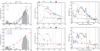 |
Fig. 15 Comparison of photometric models to HST asymmetry amplitude A40, minimum longitude ∆θmin, and the PPS optical depth τpps measurements. Both identical particle (upper frames) and W = 20 size distribution models (lower frames) are shown, for various τdyn values indicated by the legends. In all cases ϵn = 0.1 andρ = 250 kg m−3 is assumed. Filled circles indicate simulations leading to overstability. The HST measurements are from French et al. (2007). Arrows mark regions where overstable oscillations have been observed in various studies quoted in the text. |
7.3 Comparison to A and B ring occultation measurements
Although our current study concentrates on brightness asymmetry on ground-based geometries, we had a brief look at how the above favoured models for A and B ring regions compare with the Cassini opacity measurements, and wake structural analysis based on simplified slab models for the self-gravity wakes. Robbins et al. (2010) made an extensive grid of dynamical simulations with various τdyn and ρ, for two distances characterising Saturn’s B ring (a = 100 000 km) and A ring (a = 130 000 km), both with identical particles and with W = 10 size distribution. The Bridges et al. (1984) elasticity law with vc = vB was assumed. They found that all of their models yielded a quite low τphot ≲ 2.1, even for the highest τdyn = 4 accessed with simulations. They concluded that the actual τdyn must be much higher than 4 to yield the measured B-ring optical depths (or the observational lower limits in the case of the most opaque parts of the B ring). Consequently, this implied large surface density and very large estimated mass of the B ring.
However, in terms of the rh parameter, the range of parameters studied in Robbins et al. (2010) is actually quite limited, spanning the interval rh = 0.65 to rh = 1.05. The limits correspond to their simulations with ρ = 450 kg m−3, a = 100 000 km and to ρ = 850 kg m−3, a = 130 000 km. According to our surveys, this range of rh already corresponds to very strong selfgravity, and, importantly, prevents overstability from evolving. In contrast, our best matches for the azimuthal asymmetry suggest that rh is rather in the range 0.5–0.6 in the B-ring region, which is also consistent with the presence of overstability throughout the B ring and even in the inner parts of the A ring.
In Figure 17, we compare τphot versus τdyn in our identical particle models for rh =0.40, 0.58, and 0.70. The shaded regions indicate the span of τphot over the range of ring longitudes. Clearly, for weak or moderate strength of self-gravity, there is no problem for the system to achieve any high τphot. For strong self-gravity (rh = 0.70) the accessible τphot range is limited, in full agreement with the results in Robbins et al. (2010). In the figure two different elevations, B = 12° and B = 25° are shown. When wakes are strong (rh = 0.70), the τphot obtained from T via Eq. (3) becomes smaller for smaller B. Also, the variation with ring longitude increases. When wakes are weak (rh = 0.58), then τphot approaches τdyn. Finally, when wakes are practically absent (rh = 0.40) τphot can even exceed τdyn in the case of vertically flattened systems. This dependence of τphot/τdyn on τdyn, B and H/R in the non-gravitating limit was explored in detail in Salo & Karjalainen (2003).
Figure 18 shows the transmitted fraction T (upper row) and the corresponding τphot (lower row) versus elevation for two of the W = 20 size distribution models shown in Fig 15. They are selected to represent our preferred models for the B ring and A ring, with rh = 0.58, τdyn = 2.2 and rh = 0.68, τdyn = 1.0, respectively. The two curves denote the minimum and maximum over ring longitudes. Also shown are the same UVIS observations, which were used in the comparisons of Robbins et al. (2010). Clearly, for both A and B rings the overall correspondence of models to occultation observations is reasonably good.
7.4 Slab-model wake parameters
It is also of interest to compare the above B and A ring simulation models to the self-gravity wake parameters deduced from Cassini occultation profiles, done in terms of idealised geometric models. For example, the analysis of UVIS occultations in Colwell et al. (2006) described the local ring structure with an alternating sequence of dense wakes and rarefied interwake regions, modelling the wakes as parallel, infinitely long slabs with a rectangular cross-section, separated by some fixed distances (‘granola bar’ models). The interpretation of VIMS occultations in Hedman et al. (2007) followed a rather similar strategy, except for assuming elliptical rather than rectangular cross-section. The fitted functions for rectangular and elliptical cross-sections are (Colwell et al. 2007; Hedman et al. 2007)
![$T = {T_{{\rm{gap }}}}\left( {1 - {H \over \lambda }{{\sin \left| {\theta - {\theta _{\rm{w}}}} \right|} \over {\tan |B|}}\left[ {1 + {w \over H}{{\tan |B|} \over {\sin \left| {\theta - {\theta _{\rm{w}}}} \right|}}} \right]} \right),$](/articles/aa/full_html/2025/03/aa52328-24/aa52328-24-eq28.png) (23)
(23)
![$T = {T_{{\rm{gap }}}}\left( {1 - {H \over \lambda }{{\sin \left| {\theta - {\theta _{\rm{w}}}} \right|} \over {\tan |B|}}{{\left[ {1 + {{\left( {{w \over H}{{\tan |B|} \over {\sin \left| {\theta - {\theta _{\rm{w}}}} \right|}}} \right)}^2}} \right]}^{{1 \over 2}}}} \right).$](/articles/aa/full_html/2025/03/aa52328-24/aa52328-24-eq29.png) (24)
(24)
Here, T ≡ T(θ, B; H/λ, w/λ, Tgap, θw) is the total transmission through ring longitude θ at elevation angle B; H and w stand for the vertical thickness and radial width of the wakes, λ for the spacing between wake centres, Tgap = exp(−τgap / sin B) is the transmission through gaps, and θw is the ring longitude where wakes are seen end-on. These formulae assume that the wakes are so dense that no light is able to penetrate through them. Denoting by S /λ = 1 − w/λ the width of the gaps, the former equation corresponds to Eq. (4) in Colwell et al. (2007).
We have fitted the transmission profiles of the simulations shown in Fig. 18 to both of these equations, to obtain the parameter values shown as labels in the figure. In our fit, seven elevation angles, each with 19 equally spaced ring azimuths, were used. Except for the aspect ratio H/w, both fit functions gave nearly identical parameter values; inspection of the implied wake shapes (see Fig. 21 below) shows that the difference in thickness follows just from the different geometrical meaning of the parameter. Although the cross-section of simulated wakes is closer to elliptical, we report the rectangular cross-section parameters as they have been preferentially used in literature.
Our simulation models have a good qualitative agreement with the granola bar fits made in Jerousek et al. (2016) to Cassini UVIS and VIMS occultation measurements. For the A ring, our modelled wakes are a bit too vertically thick, having H/w = 0.31 compared to measured H/w = 0.2–0.25 (see Fig. 7 in Jerousek et al. 2016). Likewise, the gaps in our model are somewhat more opaque (τgap = 0.22 compared to the measured τgap = 0.1–0.15), which is compensated for by larger gap widths (S/W = 2.1 compared to measured S/W ≈ 1.5). In contrast to A-ring models, the simulated B-ring wakes are much flatter (H/w = 0.08) and the gaps are narrower and more opaque, qualitatively consistent with Fig. 8 in Jerousek et al. (2016).
More detailed photometric modelling and comparisons to UVIS and other datasets, taking accurately into account the optical depth, distance, and occultation geometry, are left for a future study. In any case, the current models reproduce the observations much closer than the models in Robbins et al. (2010), supporting our view that the strength of self-gravity wakes in Saturn’s rings is significantly weaker than implied by the parameter range assumed in their study.
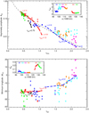 |
Fig. 16 French et al. (2007) HST measurements, A40 (upper frame) and ∆θmin (lower frame) plotted as a function of τpps. The measurements (both Beff = 10° and 15°) are colour-coded according to the ring regions B1-B4 and A1-A2 defined in Colwell et al. (2009); see the insert frames. Thick dashed lines indicate B = B′ = 12° photometric models with W = 20 size distribution, for τdyn = 0.75, 1.0 and 2.2. The thin dashed line in the upper frame corresponds to simple estimate A40 = 0.3T /(1 − T) discussed in the text. |
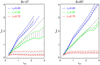 |
Fig. 17 Comparison of simulations with different values of rh, for two elevation angles. The relation between τphot and τdyn depends on the strength of gravity wakes. The shaded region corresponds to a range of τphot for different ring longitudes; the thick dashed line corresponds to ring ansae. Identical particles with ϵn = 0.1 were assumed. |
7.5 Implications for ring viscosity
In Sect. 6, we compared in Fig. 13 the rh dependence of asymmetry amplitude and viscosity (normalised by R2Ω) in simulations with different dynamical parameters. Figure 19 displays the same quantities but now converted to dimensional form. For the W = 1 and W = 20 runs with self-consistent gravity, rh is converted to Saturnocentric distance a by assuming ρ = 250 kg m−3, which was found to give the best match to HST asymmetry amplitude at a = 129 000 km. For hybrid runs with Ωz/Ω = 4.4 and 7.5, ρ = 450 kg m−3 and 750 kg m−3 are assumed, respectively; these values are chosen to match the A40 amplitude profile in hybrid models to the self-consistent W = 1 model (left frame). After converting to dimensional quantities the order of νɡrav curves is reversed compared to Fig. 13: the implied νɡrav in hybrid models increases with the assumed Ωz/Ω when ρ is chosen to match the asymmetry amplitude (middle frame).
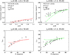 |
Fig. 18 Models for the B ring (rh = 0.58, τdyn = 2.2, left) and the A ring (rh = 0.68, τdyn = 1, right) transparency versus elevation. The upper frame shows the transmission fraction T over sin B, as in Robbins et al. (2010), while the lower frames display the same as τphot versus B, following Colwell et al. (2007). Curves correspond to modelled maximum and minimum transmission over full range of ring longitudes. Size distribution models with W = 20 and ϵn = 0.1 were used. Points stand for B and A ring UVIS occultation data for different ring longitudes, traced from Figs. 5 and 6 in Robbins et al. (2010). Original UVIS data from Colwell et al. (2006, 2007). |
7.5.1 B ring
A constant surface density, Σ = 650 kg m−2, is used in Fig. 19 (middle frame), representing a typical value of B ring surface density (Hedman & Nicholson 2016). For other choices, the νɡrav and νtot would scale by a factor (Σ/650 kg m−2)2. Although the curves are based on τdyn = 1 simulations, they apply to other τdyn’s as well. For example, assuming a larger τdyn would not change the implied νɡrav if Σ is kept fixed, although in the non- dimensional form gravitational viscosity has a  dependence. Namely, for a given Σ, increasing τdyn requires R ∝ 1/τdyn, exactly cancelling the increased τdyn. The same is directly seen from the dimensional form of νɡrav, Eq. (15). In principle, the other viscosity components may have different τdyn dependence, but Fig B.1 implies that in practice the νtot /(R2 Ω) follows more or less the same τdyn dependence.
The values of νtot (Fig. 19, right frame) implied by the different simulation models, including the hybrid simulations, all fall into the interval (10–40) ⋅ 10−4 m2 s−1 in the B-ring region. This range is much narrower than that of νɡrav. Such a difference follows from the dominant role of nonlocal viscosity in this weak self-gravity regime. For the A-ring region, the corresponding νtot range in the figure is (20–60) ⋅ 10−4 m2 s−1, assuming a mean Σ = 350 kg m−2 (Tiscareno & Harris 2018). For the A ring, the νtot follows closely the νɡrav as the nonlocal contribution is minor so that νtot ≈ 2νɡrav. The simulated B-ring viscosities, based on our asymmetry amplitude matching agree well with ν = (24– 30) ⋅ 10−4 m2 s−1 estimated in Tajeddine et al. (2017), based on balancing the viscous angular momentum flux with the torques exerted at various first order satellite resonances (dashed blue line in the right frame).
7.5.2 A ring
Figure 20 shows a more detailed comparison to A-ring viscosity measurements. In the left frame the symbols denote the Tiscareno et al. (2007) measurements of A ring viscosity, which were based on fitting the damping of density waves associated with weak satellite resonances. According to these measurements, the ring viscosity rises by about a factor ∼10 from the inner to mid A ring (a = 125 000 to 132 000 km). The same measurements also gave estimates of the A-ring surface densities at the same locations, fitted with a linear rise from about 350 to 450 kg m−2 at the above interval. The measurements are compared to νtot ≈ 2νɡrav curves from the Daisaka-formula, Eq. (15), assuming various internal densities and the same linear fit for Σ. The closest agreement is for ρ ≈ 900 kg m−3, although the measurements suggest an even steeper rise of viscosity than predicted by Eq. (15). Also note that substantial part of the model slope is due to the assumed increase in Σ with distance. Later measurements in Tiscareno & Harris (2018) in fact suggest that surface density is more nearly constant at Σ ≈ 350 kg m−2. For a fixed Σ, Eq. (15) implies νɡrav ∝ r19/2. The slope indicated by this relation is shown by the dash-dotted curve, for ρ = 250 kg m−3, being much shallower than suggested by Tiscareno et al. (2007) measurements.
The right frame of Fig. 20 shows the νtot in simulation models of Fig 19. A fixed surface density, Σ = 350 kg m−2, is adopted. In the curves for W = 1 and W = 20, ρ = 250 kg m−3 is assumed. Although the νtot exceeds by a factor of three that estimated from Eq. (15) when W = 20, it falls short of the values measured in Tiscareno et al. (2007). A somewhat larger νtot is obtained in hybrid simulation models, which assume a larger ρ in order to match the A-ring peak asymmetry amplitude. Nevertheless, the simulated viscosities are in all cases substantially smaller than implied by Tiscareno et al. (2007) measurements.
Indeed, as is discussed in detail in Tajeddine et al. (2017), it is likely that the viscosities measured from density wave damping are not representative of the viscosities in non-perturbed regions, such as the ones that our local simulation models refer to. In their study Tajeddine et al. (2017) estimated much smaller viscosities (marked with shaded region) for the A ring, with maximum values ∼50 ⋅ 104 m2/s at a = 125, 000 km, falling gradually to about 20 ⋅ 104 m2/s at a = 132 000 km – a value an order of magnitude less than obtained from the damping of density waves at resonance locations. Our simulated values are comparable, though they show an opposite trend with distance.
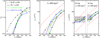 |
Fig. 19 Similar to Fig. 13 except using dimensional values for viscosities. Left frame: A40 vs distance a, assuming ρ = 250 kg m−3 for self-consistent runs with W = 1 and W = 20, and 450 kg m−3 and 750 kg m−3 in hybrid-method simulations with Ωz/Ω = 4.4 and 7.5, respectively. Middle frame: νɡrav, assuming ring surface density Σ = 650 kg m−2, representing typical B ring value (Hedman & Nicholson 2016). Dash-dotted red lines indicate Daisaka et al. (2001) formula (Eq. (14)) for νɡrav, for ρ = 250 kg m−3 and ρ = 900 kg m−3. In the right frame, the shaded regions highlight modeled total viscosities for the B and A ring regions, using Σ = 650 kg m−2 and Σ = 350 kg m−2, respectively. Dash-dotted red curves stand now for Daisaka et al. (2001) formula with νtot = 2νgrav. The dashed purple curve indicates the B ring viscosity estimated in Tajeddine et al. (2017). |
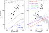 |
Fig. 20 Comparison to Tiscareno et al. (2007) and Tajeddine et al. (2017) estimates of A-ring viscosities. Left frame: symbols denote viscosities measured from damping of density waves (Tiscareno et al. 2007), while dashed lines show νD, the Daisaka et al. (2001) formula estimates (Eq. 14) assuming different internal densities of particles, ρ = 250, 450, and 900 kg m−3). In these estimates the same linear trend Σ = 337 + 13 × (a − 124) is adopted as in Tiscareno et al. (2007), where Σ is in units of kg m−2 and a in units of 1000 km. For comparison, the dash-dotted line uses a fixed Σ = 350 kg m−2 (Tiscareno & Harris 2018). Right frame: simulated total viscosities for the same models and internal densities as in Fig. 19, assuming a fixed surface density Σ = 350 kg m−3. The dashed region indicates the Tajeddine et al. (2017) viscosity estimate from angular momentum flux. |
7.6 Vertical thickness of self-gravity wakes
As was described in previous sections, increasing the vertical self-gravity via using Ωz/Ω > 1 reduces the strength of selfgravity wakes. This is indicated both by reduced νɡrav and A40. The upper frame of Fig. 21 compares systems with rh = 0.70. In the case of self-consistent vertical gravity, the system develops strong wake structure as expected, but when Ωz/Ω = 4.4 or 7.5 is used, the system becomes increasingly dominated by overstable oscillations. The edge-on snapshots illustrate the strong flattening of the system with increased Ωz/Ω (note that the vertical aspect ratio is exaggerated by a factor of five). In the examples show, νɡrav/(R2Ω) = 5.67, 0.28, 0.04, respectively.
The lower frame of Fig. 21 studies the flattening of the wakes in more quantitative way, by comparing self-consistent and hybrid method simulations that lead to strong wakes with approximately the same νtot ≈ 100 – 200 ⋅ 10−4 m2/s. The self-consistent run corresponds to rh = 0.76, while the two hybrid runs have rh = 0.9 and 1.1 for Ωz/Ω = 4.4 and 7.5, respectively. In the face-on projection, the wake structure appears superficially fairly similar in all cases, although there are fewer particles in the inter-wake regions in the hybrid models with larger rh. The significant difference is again in the vertical thickness of wakes. In the simulations with enhanced vertical force the typical wake cross-section is much more flattened: slabmodels with Eq. (23) indicate H/w = 0.20 and 0.12 for the Ωz/Ω = 4.4 and 7.5 models, respectively, compared to H/w = 0.35 in the model with self-consistent vertical gravity (corresponds to effective Ωz/Ω = 2.5). More flattened profile leads to reduced planar forces exerted by the wakes, with a reduction roughly proportional to H/w, here compensated by larger internal density of particles so that νɡrav is nearly the same.
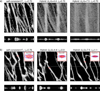 |
Fig. 21 Effect of extra vertical force on the self-gravity wakes. In a) three examples of simulation with self-consistent vertical forces (left), and with hybrid method, using Ωz/Ω = 4.5 and 7.5 (middle and right frames). A fixed rh = 0.70 is assumed. In b) similar examples for strong wakes, but with varying rh so that they yield roughly the same νtot ≈ 100–160 ⋅ 10−4m2/s, when internal densities ρ = 250 kg m−3, 450 kg m−3 and 750 kg m−3 are assumed, respectively. Note that since Σ = 350 kg m−2 is fixed, the particle size R ∝ 1/ρ. The upper frames show face-on snapshots of the system, limited to 4λcr × 4λcr regions. In the edge-on snapshots, the vertical scale is exaggerated by a factor of 5. The insert images in b) show cuts in xz plane through the positions indicated by the short vertical bars in the upper frames. The blue rectangles and ellipses indicate the size and shape of the fitted slab models, using Eqs. (23) and (24), assuming wake separation λ = λcr; the labels indicate the wake’s height/width ratio for Eq. (23). The vertical projections in the lower frames are calculated by sampling only particles around the grey y = 0 line marked in the upper snapshots. |
7.7 Outer A-ring asymmetry: Suppression by debris
As is seen in models of Fig. 15, the steep rise of amplitude from inner to mid A ring can be at least partly accounted for as a transition from overstable system to a system with strong wakes, taking place in a rather narrow interval of rh. The behaviour is similar in all self-consistent models as well in the hybrid simulations, although the exact rh range depends on the model. By choosing an appropriate internal density, the rh transition can be matched with the inner A-ring region. On the other hand, the rapid decline of asymmetry in the outer A ring remains problematic as the degradation of wakes to particle clumps takes place over quite a broad rh interval, when fixed particle properties are assumed. The same applies to both self-consistent and hybrid models. A promising possibility is that particle properties or the size distribution vary at the outer A ring. According to our simulations, small changes in τdyn or ϵn would have a rather minor effect. In contrast, the width of size distribution has a dramatic effect on the strength of asymmetry in the strong wake regime, even if the underlying wake structure is not much affected. Rather, the reduction of asymmetry then follows from small particles hiding the wakes by increasing optical depth of the inter-wakes gaps, τgap. An even more efficient way to reduce the asymmetry would be an increased contribution of more uniformly distributed population of small particles, accounting also for the increased optical depth at the outermost A ring.
An interesting question is what might cause sufficiently large change in W or/and τgap. A candidate mechanism, already proposed in Salo & Schmidt (2007), is a release of small debris grains from the surfaces of regolith-covered ring particles due to increased maximum impact velocities when self-gravity gets stronger. Namely, as rh increases, the distribution of impact velocities acquires a high velocity tail, due to splashing together of wake filaments: a nice illustration of such splashing is provided by Ohtsuki et al. (2020)3.
Following a fully self-consistent dynamical model of regolith covered particles, with the release and re-absorption of debris, is beyond our computational capacities. Therefore, we have devised a simple toy-model for the release of debris and its influence on brightness asymmetry. The model is based on tabulating the distribution of impact velocities in a series of self-consistent dynamical simulations performed for different distances, and adding a uniformly distributed debris population to particle snapshots stored from the simulations. The chosen optical depth of the debris population varies from simulation to simulation, depending on the amount of high-velocity impacts. We assume that release of debris takes place in fast particle impacts with vn > vthresh, detaching the regolith layers normally attached to the surfaces of impactors. Furthermore, we assume that the debris grains are rapidly re-absorbed in subsequent impacts with ring particles. This leads to steady-state debris distribution, with an optical depth of
 (25)
(25)
where fimp and ffast denote the impact frequency and the frequency of fast impacts, and τregolith is the total optical depth of the regolith grains bound to particles. We furthermore assume that the total optical depth of regolith particles, normally attached to particle surfaces, is a factor Y times larger than τdyn. The factor of 4 in the equation follows from different cross-section for impacts in particle-particle and particle-debris impacts.
Examples of such a toy model are shown in Fig. 22, using two different ad hoc values, vthresh = 0.5 and 1.0 cm/s: for one- metre particles these correspond to ∼(25–50)RΩ, much larger than the escape velocities of ring particles, or typical mutual velocities inside wakes. With increased distance, the relative amount of fast impacts increases rapidly as the increasingly strong wakes develop and frequently splash against each other. For vthresh = 0.5 and 1.0 cm/s this happens for a ≳ 120 000 km and a ≳ 130 000 km, respectively. The underlying dynamical model is similar to the τdyn = 0.5, ρ = 450 kg m−3 models in French et al. (2007), yielding a broad A40 maximum at the mid A ring. With the inclusion of debris population, the asymmetry amplitude is suppressed, with the degree of suppression depending on the assumed parameters vthresh and Y. Clearly, such a model could at least in principle explain the observed decay of asymmetry at the outer A ring.
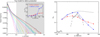 |
Fig. 22 Toy-model for suppression of azimuthal asymmetry due to impact-released debris. The frame in the left shows the distribution of impact velocities in a series of dynamical simulations, performed with τdyn = 0.50, ϵn = 0.5, for rh = 0.72–0.98. Assuming ρ = 450 kg m−3, this corresponds to Saturnocentric distances 110–150 000 km. Shaded regions indicate the frequency of impacts with vn greater than 0.5 and 1.0 cm s−1 : their relative amount increases rapidly, while the mean of impact velocity is nearly constant with distance. The modelled A40 amplitudes are shown in the right frame with a dashed line, while the grey points denote the HST measurements. The red and green curves indicate toy-models with different values for the parameters vthresh and Y: the insert in the left frame displays the amount of free debris as a function of distance following from Eq. (25), while the curves in the right indicate A40 amplitudes in photometric models where the uniform debris population has been added. |
8 Summary and discussion
We have carried out a reasonably thorough survey of the effects of the main dynamical parameters (rh, ϵn, τdyn, W) on the expected photometric properties of self-gravitating planetary rings, together with observational comparisons, mainly to HST azimuthal asymmetry measurements. Compared to similar modelling and comparisons made in Salo et al. (2004); French et al. (2007), the range of dynamical models has been significantly expanded, due to the maximum number of simulation particles increasing one hundred-fold, thanks to our use of the new multiprocessor SoftIS code (Mondino-Llermanos & Salo 2022). However, our impact model does not include adhesive forces between particles, which could, in principle, shift the regime in which self-gravity wakes suppress overstability to significantly larger rh values, as is shown by Ballouz et al. (2017). To mimic such effects, we augmented our fully self-consistent simulations with the hybrid simulations introduced in Mondino-Llermanos & Salo (2023). In these simulations, the vertical force is described with an enhanced vertical frequency, Ωz/Ω > 1, combined with self-consistently calculated planar self-gravity. Enhancing the vertical force leads to a vertically more flattened cross-section of wakes compared to those with self-consistent vertical gravity; this flattening weakens the planar component exerted by the wakes, leading to qualitatively similar shifts in behaviour with respect to rh, as is seen by Ballouz et al. (2017).
8.1 Parameter surveys
The dynamical simulation survey over the rh parameter, measuring the strength of self-gravity relative to central shear, indicates a relatively rapid but still smooth transition from overstability-dominated systems to wake-dominated ones. With our standard identical particle model (τdyn = 1.0, ϵn = 0.1, W = 1), the system becomes overstable at rh ≈ 0.5, while for rh ≳ 0.65, inclined self-gravity wakes suppress overstable oscillations (Mondino-Llermanos & Salo 2023). The presence of overstability throughout the B ring and also in the inner A ring sets a strong observational constraint for the strength of self-gravity in Saturn’s rings when identified with this range of rh parameter.
In the strong wake regime (rh ≳ 0.65), photometric models indicate that the overall ring brightness drops as the gaps between wakes reduce the reflecting area. The I/F becomes also longitude-dependent, since at a slanted view the visibility of gaps depends on the viewing direction with respect to the mean direction of wakes. In our standard identical particle model, the amplitude of brightness variations reaches a maximum Aasym ≈ 0.6 at rh = 0.80 (see Fig. 4). For even larger rh, the increased twisting and clumpiness reduces Aasym, and eventually self-gravity wins over the shear and the wakes collapse to gravity-bound aggregates (see Fig. 23 in Salo et al. 2018). Similar behaviour is seen in τphot calculated from the line-of- sight transparency. In the overstability-dominated regime, the asymmetry amplitude is small, only a few percent. At the transition from overstability to wakes, the ring longitude of minimum I/F changes from ansa to roughly 20° before the ansa. This behaviour is accordance with the picture sketched in Fig. 3.
For rings with more elastic particles, the behaviour with rh is qualitatively similar compared to ϵn = 0.1, but delayed to larger rh’s (see Fig. 7). For ϵn = 0.5 or for ϵn(vn) with vc/vB = 1 the shift is very small, but if the steady-state velocity dispersion is larger (the case vc /vB = 5 in the figure) the delay is substantial. The maximum asymmetry amplitude also drops, and importantly, such a system does not exhibit overstability at any rh. In the above-mentioned hybrid method simulations the delay in evolution with rh increases with increasing Ωz/Ω. This is true both for the transition from overstable to wake-dominated systems, and for the value of rh corresponding to maximum Aasym. For Ωz/Ω ≳ 2 hybrid simulations lead to overstability even at the limit rh → 0.
Overstable oscillations arise only when the central plane filling factor FF (0) exceeds a critical value: FF(0) ≳ F Fcrit, where F Fcrit ≈ 0.45 in the non-gravitating or weakly gravitating case (Rein & Latter 2013), decreasing to F Fcrit ≈ 0.39 when rh increases from 0.2 to 0.65 (Mondino-Llermanos & Salo 2023). Up to rh ≈ 0.4, the reduction of F Fcrit stems from increased vertical self-gravity, whereas beyond that planar gravity further promotes overstability by reducing F Fcrit (see Fig. D1 in Lehmann & Salo 2024 and Fig. C1 in Mondino-Llermanos & Salo 2023). These critical filling factors are achieved when τdyn exceeds a threshold value that depends on the vertical extent of the system.
In contrast to overstability, self-gravity wakes do not have any threshold density, but they grow gradually in strength with increasing τdyn and rh. A convenient measure of the wake strength is given by gravitational viscosity, νɡrav. At low τdyn ≲ 0.5, the stronger wakes always lead to larger Aasym (see Fig. 9). However, for larger τdyn the behaviour differs between strong (rh ≳ 0.65) and weak (rh ≲ 0.65) self-gravity regimes: in the former case Aasym grows until saturating for τdyn ≳ 1.5 whereas in the latter case Aasym drops with τdyn. This drop is due to development of overstability once the threshold τdyn ∼ 0.7 is exceeded: in the case of overstability, the density contrast between density maxima and minima is never as large as in the case of wakes. The longitude of I/F minimum depends also sensitively on τdyn, corresponding to wake pitch angles ϕw ∼ 30° at the limit τdyn → 0. For τdyn ≳ 1.5 the inferred ϕw varies from 0° – 10° (prominent overstable oscillations) to 15° – 25° (prominent wakes).
The inclusion of an extended size distribution can have a drastic effect on the behaviour of the simulation system. Again, the effect in strong and weak self-gravity regimes differ: in the former case a larger width of the distribution reduces Aasym although the wake structure remains strong, while in the latter case the system can shift from overstability-dominated system to a wake-dominated system, leading to enhanced Aasym. The effective pitch angle ϕw increases significantly with the width of the size distribution.
8.2 Anomalous asymmetry
An unexpected finding in current simulations and photometric models was that also non-gravitating and weakly self-gravitating systems (rh ≲ 0.4) can exhibit longitude variations in I/F and τphot. In this case, the minimum longitude is shifted to after the ring ansa, indicating the presence of leading particle enhancements. However, the amplitude of I/F variation is small, just ∼0.01 for ϵn = 0.1, explaining why such a phenomenon has escaped earlier attention. Autocorrelation analysis confirms that the origin of this ’anomalous’ asymmetry is in the temporary crowding of particles at the leading quadrants with respect to shear. In retrospect, it is easy to understand the presence of such mild polarisation in a low velocity dispersion ring, arising due to combination of shear flow and the substantial reduction of relative velocities in impacts, which occur preferentially in the leading quadrants. When velocity dispersion is larger, the distribution of impact directions gets more isotropic and the effect disappears. Such polarisation is present also in more strongly self-gravitating systems, but its effect is completely washed out by the axisymmetric overstable structures and eventually by the trailing wakes (see Fig. 6). Also, for dynamically hotter systems the effect decreases rapidly, with amplitude proportional to (H/R)−1.
We examined the question of whether such leading features could be detected in Saturn ring observations; for example, in the C ring, where the strength of self-gravity wakes is expected to be negligible. However, the small expected amplitude makes it implausible that such brightness variations could be separated from other variations; for example, due to Saturn-shine; the longitude dependent illumination by Saturn’s globe that becomes important close to the planet (see Dones et al. 1993). The prospects are better in occultation measurements, as the τphot variations can be even of the order of 20%. Since the modelled amplitude of variations depends strongly on ring velocity dispersion via ϵn, detecting (or ruling out) such variations could in principle offer a diagnostic for estimating the local ring thickness.
8.3 Ring viscosity
In the case of strong wakes the main contributions to ring viscosity arise from gravitational viscosity and the local viscosity, which in turn is closely connected to the systematic motions induced by the wakes. The standard fitting formula from Daisaka et al. (2001) assumes νl ∼ νɡrav and νtot ∼ 2νɡrav, in agreement with our simulations (see the rh = 0.8 case in Fig. 12). However, the actual magnitude of νɡrav can be even a factor 2–3 larger than implied by this formula, for example in the case of an extended size distribution (see Appendix A). In the weak gravity regime, and in particular if ϵn is small or if the hybrid method with Ωz/Ω>>1 is used, νnl may also dominate, in which case νtot>>νɡrav (see rh = 0.61 case in Fig. 12). Nevertheless, for Saturn’s A ring with a prominent wake structure the measured total viscosity should be a close proxy to νɡrav. On the other hand, in the B ring, the presence of overstabilities indicates that non-local viscosity is dominant: simulations in Mondino-Llermanos & Salo (2023) indicate that wakes suppress overstability if νɡrav ≳ 0.4νnl. A similar limit applies to hybrid method simulations and to simulations with a self-consistent vertical field.
8.4 Comparison to Hubble Space Telescope data
We have carried out a systematic comparison of our photometric models with the extensive HST dataset in French et al. (2007). These observations provide simultaneous coverage of the full range of Saturnocentric radii with a uniform observing geometry, ideal for comparison with the simulated radial trends in asymmetry amplitude and the longitude of the brightness minimum. The radial resolution of the HST observations, ∼1000 km, does not allow for the spiral density waves to be resolved, although the strongest waves induce a local dip in amplitude and a small shift in the ∆θmin profiles (see Fig. 21 in French et al. 2007, showing the effect of the Janus 4:3, Janus 5:4, and Mimas 5:3 density waves). Most likely, the overall effect of underlying unresolved density waves is very small, supported by the fact that the trends in ∆θmin in the HST imaging data agree very well with similar trends in UVIS and VIMS stellar occultation observations (see Fig. 57 in Salo et al. 2018). We may thus safely assume that the HST data provide a reliable signature of the wake structure as it appears in the unperturbed regions of Saturn’s rings.
Our re-analysis of French et al. (2007) HST asymmetry observations suggests even smaller internal density, ρ ∼ 250 kg m−3, than the value ρ ∼ 450 kg m−3 preferred in French et al. (2007). The difference follows from extending the models to larger optical depth (τphot = 1 instead of 0.5) and using more dissipative particles (ϵn = 0.1 instead of 0.5; see Fig. 14).
With ρ = 250 kg m−3 the asymmetry peak at 129 000 km corresponds to rh ∼ 0.7, indicating strong self-gravity wakes. Likewise, the inner A-ring region with observed overstability (a = 124 000 km) corresponds to rh ∼ 0.65, which according to simulations is about the largest value where overstability can take place. With the same ρ, the inner edge of the B ring (92 000 km) corresponds to rh = 0.5, still marginally in the overstable regime.
The inclusion of a size distribution improves the match to observations significantly. In the A ring at a = 129 000 km, the modelled ϕw ∼ 17° for single-sized particles with τdyn ∼ 1, which is ∼4° smaller than observed4. This disagreement disappears with W ∼ 20, which yields ϕw ∼ 21°. A radial trend in W, in the sense that W decreases with a could account for the otherwise puzzling systematic gradient in observed ϕw, which decreases 24° → 20° between a = 125 000 km and a = 130 000 km. This is seen in Fig. 15 for B = 12°; observations show exactly the same gradient for all elevation angles (see Fig. 20 in French et al. 2007). According to photometric models in Fig. 12 such a change could occur if W = 50 → 10. Such a change in W would also steepen the rise of asymmetry amplitude, taking place at the same a interval.
For the B ring with weak self-gravity, the modelled asymmetry amplitudes are much stronger when W = 20 size distribution is included, and agree quite well with the observed amplitudes. The fact that wakes are weak in the B ring also manifests in that asymmetry amplitude is largest when optical depth is smallest. For example, at the region a = 94 000–98 000 km, the asymmetry is very similar the A-ring asymmetry (ϕw ∼ 20–25), except for smaller amplitude. In this region τpps is of the order of unity, below the τthresh for overstability in the case of extended size distribution. On the other hand, at a = 110 000–114 000 km, τpps ∼ 1.5–2, so that wakes embedded with overstability are expected; indeed the observed Aasym is smaller and ϕw ∼ 10°.
The inferred small internal density of particles is quite a robust result in models where only self-gravity is considered, not likely to be altered if an even larger range of τdyn, ϵn or W combinations were considered than already covered by the current study. However, the possibility remains that the ring particles are strongly affected by sticking forces, in which case the particles could have significantly larger ρ. For example in terms of our hybrid model, simulations with Ωz/Ω = 4.4 and 7.5, combined with ρ = 450 kg m−3 and 750 kg m−3, respectively, lead to very similar radial Aasym profiles as the standard 250 kg m−3 model. Clearly, photometric modelling of dynamical simulations with realistic inclusion of sticking forces, like in Ballouz et al. (2017), would be desirable. Nevertheless, our modeled small internal densities are in accordance with the large porosities of ring particles (even 75–90%) inferred from microwave Very Large Array (VLA) observations (Zhang et al. 2017, 2019).
8.5 Comparison to Cassini opacity measurements
Comparison to Cassini stellar occultation measurements provided an independent check of our best fitting HST asymmetry amplitude models. We compared the photometric MC models both directly to the observed data points of ring transparency versus elevation, and to the fitted parameters derived from simplified analytical models, describing wakes as regularly spaced slabs with either rectangular or ellipsoidal cross-sections (Colwell et al. 2006; Hedman et al. 2007). For the comparisons two typical models were selected, one for weak self-gravity (rh = 0.58; B ring) and the other for strong gravity (rh = 0.68; A ring). Both comparisons gave satisfactory match, for example in the sense that the B-ring simulated wakes had more narrow and opaque gaps than the A-ring wakes, having also smaller H/w ratios (Fig. 18). We note that in our fits to dynamical simulations, MC models covering a regular grid of B and ring longitudes was used, whereas the data used in observational fits has been dictated by the geometry of available occultation profiles. Clearly, a future comparison to specific occultation geometries would be desirable.
Perhaps the most important conclusion from our photometric transparency models is that there is no principal problem in matching the high τphot in the B ring, as long as self-gravity is weak (rh ≲ 0.6). In this case τphot ∼ τdyn. In earlier simulation modelling (Robbins et al. 2010) unrealistically strong wakes in B ring were assumed, leading to the conclusion that the underlying τdyn must be extremely high.
8.6 Comparison to Saturn ring viscosity estimates
We also checked what are the predicted kinematic viscosities of the models best matching the HST asymmetry data. To account for the possibility that the actual internal density is higher than the ρ = 250 kg m−3, also hybrid models with larger ρ we included. The implied viscosities for the B ring were in range νtot = (10–40) ⋅ 10−4 m2 s−1, when adopting a typical B-ring surface density of Σ = 650 kg m−2 (Hedman & Nicholson 2016). Similarly, using Σ = 350 kg m−2 (Tiscareno & Harris 2018) for the A ring gave νtot = (20–60) ⋅ 10−4 m2 s−1. The B-ring values agree quite well with the results in Tajeddine et al. (2017), whereas our A-ring values are nearly a factor of ten smaller than the measurements in Tiscareno et al. (2007). On the other hand, Tajeddine et al. (2017) obtained values which are comparable or even lower than our values toward the outer part of the A ring. Tajeddine et al. (2017) attributes the difference compared to Tiscareno et al. (2007) to the difference in viscosities in perturbed versus non-perturbed ring regions. Indeed, a better agreement to Tajeddine et al. (2017) is to be expected, as our local simulation values correspond to non-perturbed ring shear flow.
Interestingly, the Tiscareno et al. (2007) measurements for resonance regions indicate a slope of νtot which is considerably steeper that the distance-dependence predicted for νɡrav - dominated total viscosity. One possibility that would bring the slope down is that the inner A-ring viscosities are in fact underestimated. Namely, according to Schmidt et al. (2016), near the overstability-boundary the viscous damping of density waves is not as efficient as assumed by the standard formulas: density waves can have very long damping lengths, or in fact be overstable. This could lead to a too small viscosity estimate at the region a = 125–126 000 km explaining the very strong slope, though not explaining why the viscosities derived for resonance sites are so high to start with.
Another hypothetical way to increase the νtot slope would be to assume that the importance of particle sticking depends on distance. Let’s assume that in the inner A ring the adhesion is sufficient to keep the wakes vertically flattened, even if the particles had a internal density close to solid ice. This small H/w aspect ratio would reduce the strength of planar self-gravity and keep gravitational viscosity small. Let’s further assume that with increasing distance, sticking forces would gradually lose their hold, so that the wakes transform back to a less flattened state, like our self-consistent wakes in the absence of any extra vertical force. This increases the strength of wakes and thus also νɡrav. For example, with ρ ∼ 900 kgm−3, the viscosity in the mid A ring would then be about tenfold compared to that for the ρ = 250 kgm−3 model in Fig. 20, or close to what was measured by Tiscareno et al. (2007). Such a scenario would also help to increase the slope of asymmetry amplitude in the inner to mid A ring, and moreover a particle density close to solid ice would also bring the outer edge of rings close to the classical Roche limit. However, the above-mentioned small but systematic reduction in the effective ϕw in the region a = 125 000–130 000 km would be difficult to reconcile with this scenario. Namely, the effect of moving from the hybrid model to the self-consistent model while keeping ρ (rh) fixed should increase the ϕw (see Fig. 7), contrary to what is seen in observations.
8.7 Debris release from regolith-covered ring particles
In Sect. 7.7, a toy-model for the suppression of azimuthal asymmetry in the outer A ring was examined, based on hiding the self-gravity wakes with a population of small debris particles. The debris was suggested to originate from surface regolith grains released in high-velocity impacts between particles when shearing gravity wakes collide. The fraction of fast impacts increases with distance, resulting in similarly increasing steadystate background τdebris. Exact values in our toy-model depend on the assumed threshold velocity for debris release and amount of regolith material released. With background τdebris ∼ 0.2–0.3 substantial drop in asymmetry is in principle possible. Such values fall on the range of theoretical models in Bodrova et al. (2012), where adhesion and release of debris in impacts were described in terms of bimodal carrier particle/debris particle populations. An increased amount of sub-cm particles for the outermost A ring have also been inferred from UVIS stellar (Becker et al. 2016; Jerousek et al. 2016) and VIMS solar occultation studies (Harbison et al. 2013).
A quite similar debris-release toy-model was found to be essential for a successful match of the I/F of A-ring propeller features in Sremčević et al. (2007). In that case the enhanced impact velocities were assigned to moonlet-induced perturbations. Likewise, in Salo & Karjalainen (2003) a simple model in terms of increased number of small particles in the vicinity of Mimas 5:3 density wave explained successfully the observed (Dones et al. 1993) contrast reversal between low and phase angle observations.
9 Conclusions
The presented dynamical and photometric models, though by no means fully satisfactory, provide useful insights into the self-gravity wakes and overstabilities in Saturn’s rings.
The comparison of gravity-only models to HST measurements in French et al. (2007) suggested a low internal density of particles, ρ ∼ 250 kg m−3. With the inclusion of size distribution, both the inner B-ring azimuthal asymmetry and the steep rise of asymmetry amplitude in mid A ring can be accounted for.
The same models agree well with the Cassini opacity measurements (Colwell et al. 2007). Most importantly, the problem in explaining the high photometric optical depth of the B ring (Robbins et al. 2010) is shown to be due to assuming too strong a wake structure in this ring.
A larger ρ closer to the one of solid ice is possible if there are additional forces leading to vertically flattened and thus weaker self-gravity wakes. Such a flattening could be attributed to adhesive forces that are counteracted by shear in planar directions but not in the vertical. Our hybrid simulations with enhanced vertical forces lead in this respect to similar behaviour as the simulations of Ballouz et al. (2017), which included sticking forces between particles.
The weakness of self-gravity wakes in the B ring is evidenced by the fact that viscous overstabilities have been observed throughout the ring. This implies that gravitational viscosity is not a dominant source of viscosity in the B-ring region. The estimated B-ring viscosity is νtot = (10–40) ⋅ 10−4 m2 s−1, assuming a typical surface density, Σ = 650 kg m−2. This agrees well with estimates made in Tajeddine et al. (2017).
Self-gravity wakes are strong in the mid and outer A ring. The estimated A-ring viscosity is νtot = (20–60) ⋅ 10−4 m2s−1, assuming a surface density of Σ = 350 kg m−2. Compared to estimates based on damping of weak density waves (Tiscareno et al. 2007), our simulated viscosities are about a factor of ∼10 smaller. They are closer to estimates by Tajeddine et al. (2017), although the simulated trend of increased ν with distance is opposite to their estimate.
For the suppression of asymmetry in the outer A ring, a simple toy model of increased impact-released debris is suggested. In this model, the wakes are still dynamically strong but shrouded by the small particle background.
In dynamically cold simulation systems, auto-correlation analysis reveals a tendency for weak shear-induced leading density enhancements. Their photometric signature is weak and easily hidden by axisymmetric overstable oscillations and/or trailing self-gravity wakes. If observable, this might provide a diagnostic tool for estimating the ring velocity dispersion.
Combining dynamical and photometric simulations is a powerful way to model the unresolved fine structure in Saturn’s rings. The puzzling fact that gravity-only models imply such low internal particle densities emphasises the need for similar modelling in the case in which particle-particle sticking forces are realistically included. Also, changes in the size distribution should be allowed in a self-consistent way. An obvious further extension would be to apply similar photometric models to the wide range of Cassini measurements, which involve observing geometries that are far more diverse than the ones analysed in this study.
Appendix A Size distribution
In Sect. 5 we performed simulations with a q = 3 power-law size distributions, with varied W = Rmax/Rmin. In each set of simulations with varied W, the dynamical optical depth and surface density were kept constant, which was achieved by the proper choice of particle number and size range.
Let’s denote by R0 and N0 the radius and number of particles in the case of identical particles, corresponding to τ0 and Σ0. For identical particles
 (A.1)
(A.1)
where the area of the simulation region A = LxLy and ρ is the internal density of particles. We fix q and want to change W while keeping the τ and Σ fixed to the above values, which requires that Rmin, Rmax, and N are modified. The power-law size distribution is defined as
 (A.2)
(A.2)
where dN/dR is the number of particles in size range [R, r + dR] and C0 is a normalisation constant determined by the total number of particles in the simulation. For this distribution
 (A.3)
(A.3)
 (A.4)
(A.4)
 (A.5)
(A.5)
where the shorthand abbreviations stand for
 (A.6)
(A.6)
Setting τ and Σ to same values as for identical particles yields
 (A.7)
(A.7)
from which Rmax /R0 is obtained. Inserting this ratio and the normalisation constant C0 solved from Eq. A.4 to Eq. A.4 yields the N/N0 ratio. Altogether we have
 (A.8)
(A.8)
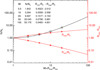 |
Fig. A.1 Number of simulation particles in size-distribution runs with q=3, compared to identical particles runs. |
Figure A.1 displays the particle number and size range for q = 3 power law distributions. For convenience, the values corresponding to W = 2.5 – 100, used in simulations of Sect. 5 are given.
The realisation of the particle size distribution is made by choosing the radii of N particles, Ri = Rmin, …, Rmax with the formula
![${R_i} = {\left( {{{(i - 1)} \over {N - 1}}\left[ {R_{\max }^{(1 - q)} - R_{\min }^{(1 - q)}} \right] + R_{\min }^{(1 - q)}} \right)^{1/(1 - q)}}\quad i = 1, \ldots ,N$](/articles/aa/full_html/2025/03/aa52328-24/aa52328-24-eq40.png) (A.9)
(A.9)
We note that we do not use random numbers but use smooth increments between particle radii: this avoids spurious variations between runs caused by slightly different numbers of the largest particles.
Appendix B Calculation of viscosities
The calculation of local and nonlocal viscosity components is done following the standard method introduced in Wisdom & Tremaine (1988), extended to the case of unequal particle masses, and to the use of visco-elastic force model for impacts (see Salo et al. (2018)). We have
 (B.1)
(B.1)
where the bar denotes average over the particle ensemble and brackets stand for averaging over time. Here cx and cy stand for shear corrected-velocities of particles, where the mean shear ( ) has been subtracted. For the nonlocal component
 (B.2)
(B.2)
 (B.3)
(B.3)
where the first form applies to instantaneous impact method, while the second form the change of velocity is written in terms of impact forces. In the sum over impacts, taken over the time interval ∆T, the symbols m> and (δcy)> stand for the mass and tangential velocity change of the particle with the larger radial co-ordinate, while ∆x> is the absolute radial difference between the colliding particles. In Eq. B3, Fij> denotes the tangential component of the impact force exerted on particle j by particle i; for non-colliding particle pairs, Fij> = 0.
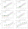 |
Fig. B.1 Viscosity measurements as a function of rh (or τdyn in the last frame) in series of simulations with different dynamical parameters. Unless otherwise indicated τdyn = 1.0, ϵn = 0.1, W = 1, rh = 0.61. Filled squares for νtot indicate runs leading to overstability. Dashed lines indicate the νgrav estimate from Eq. 14. |
The calculation of gravitational viscosity is made following (Daisaka et al. 2001),
 (B.4)
(B.4)
where |rj − rj | is the distance between particles. This equation has the same form as Eq. B.3, except for replacing impact forces with gravity. In principle, calculating Eq. B.4 is quite time-consuming as it contains a double summation over all particles. However, in tree-method utilised by SoftIS the collection of νɡrav can be done simultaneously with the construction of gravitational forces.
Besides Eq. B.4 we also utilised the autocorrelation function in estimating the gravitational viscosity. We may write
 (B.5)
(B.5)
where ζ2D is the normalised autocorrelation function of density, and Σ0 is the mean density of the system,

In practice this provides a much faster way of estimating νɡrav since the integration over the autocorrelation function needs to be done only once. This formula applies also in the case of size distribution: examples of νɡrav calculated with Eqs. B.4 and B.5 were given in Fig. 12, indicating quite good agreement between the methods.
Figure B.1 collects viscosity measurements with various dynamical parameters. The three frames in the left column compare standard self-gravity runs with hybrid method simulations with enhanced Ωz/Ω = 4.4 and 7.5; in self-consistent runs the effective Ωz/Ω ≈ 2 – 2.5. It demonstrates the strong reduction in νɡrav when Ωz/Ω increases, due to vertically more flattened wakes. Flatter wakes exert weaker planar gravity compared to more circular wakes in the standard runs (see Fig. 21). At the same time, νnl is somewhat increased in the hybrid runs, but not nearly enough to compensate for the reduced νɡrav. The filled symbols in the plot indicate runs leading to overstability: clearly, the empirical condition found in Mondino-Llermanos & Salo (2023), νɡrav/νnl ≳ 0.5 for suppression of overstability by wakes applies to the hybrid runs.
The other frames in Fig. B.1 highlight the influence of ϵn, W, and τdyn. In particular, the difference between using ϵn = 0.5 and ϵn = 0.1 is very small. In the case of W = 20, the viscosities are about a factor of 2 larger for rh ≈ 0.6 - 0.7 but the difference becomes insignificant for rh = 0.8. In the case of W = 20, the νɡrav exceeds that given by Eq. 14 by about a factor of 2.
Appendix C Size distribution comparisons
Figure C.1 highlights the effect of size distribution width on weak and strong self-gravity regimes. The upper frames correspond to rh = 0.61 simulations as in Figs. 10 and 12, for W =2, 10, and 100, displaying a transition from overstable system with mild wakes to a a system with strong wakes (see the levels of the autocorrelation plot). In this transition the asymmetry amplitude first increases but saturates at W ≳ 10. Also the effective pitch angle increases from 13° to 22°.
The lowermost three frames display simulations with strong wakes (rh = 0.85) where the increase in W leads to strong reduction in asymmetry, although based on autocorrelation plot the wake amplitude itself is not affected. The shift in effective pitch angle is from 25° to 35°. The larger ϕ’s compared to simulations in Figs. 10 and 12 arise from the small τdyn = 0.5. For W = 100 the ratio λcr/Rmax ≈ 10, so that ’wakes’ are rather fragmentary collections of smaller particles around the largest particles, with large deviation from tangential direction.
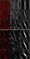 |
Fig. C.1 Examples of simulations with increases width of size distribution, W = 2, 10 and 100. In a) rh = 0.61, τdyn = 1.0 while in b) rh = 0.85, τdyn = 0.5. For each simulation the leftmost frame shows a MC ray tracing image of a typical snapshot, seen from B = 90° viewing direction and illuminated from B′= 25°. A 4λcr × 4λcr region is displayed. The middle frame displays a slice of the same snapshot through the equatorial plane, with the label indicating the A40 asymmetry amplitude calculated for the simulations. The rightmost frames shows a time-averaged surface density autocorrelation function: the label and the red line indicates the effective wake pitch angle calculated from the longitude of minimum I/F. The contour levels correspond to 10%, 30% and 50% overdensities. In all simulations ϵn = 0.1. |
References
- Ballouz, R.-L., Richardson, D. C., & Morishima, R. 2017, AJ, 153, 146 [NASA ADS] [CrossRef] [Google Scholar]
- Becker, T. M., Colwell, J. E., Esposito, L. W., et al. 2016, Icarus, 279, 20 [CrossRef] [Google Scholar]
- Bodrova, A., Schmidt, J., Spahn, F., & Brilliantov, N. 2012, Icarus, 218, 60 [NASA ADS] [CrossRef] [Google Scholar]
- Bridges, F., Hatzes, A., & Lin, D. 1984, Nature, 309, 333 [NASA ADS] [CrossRef] [Google Scholar]
- Camichel, H. 1958, Ann. Astrophys., 21, 231 [NASA ADS] [Google Scholar]
- Colombo, G., Goldreich, P., & Harris, A. W. 1976, Nature, 264, 344 [NASA ADS] [CrossRef] [Google Scholar]
- Colwell, J. E., Esposito, L. W., & Sremcevic, M. 2006, Geophys. Res. Lett., 33, L07201.1 [CrossRef] [Google Scholar]
- Colwell, J. E., Esposito, L. W., Sremcevic, M., Stewart, G. R., & McClintock, W. E. 2007, Icarus, 190, 127 [NASA ADS] [CrossRef] [Google Scholar]
- Colwell, J. E., Cooney, J. H., Esposito, L. W., & Sremcevic, M. 2009, Icarus, 200, 574 [CrossRef] [Google Scholar]
- Daisaka, H., Tanaka, H., & Ida, S. 2001, Icarus, 154, 296 [NASA ADS] [CrossRef] [Google Scholar]
- Dones, L., Cuzzi, J. N., & Showalter, M. R. 1993, Icarus, 105, 184 [NASA ADS] [CrossRef] [Google Scholar]
- Dunn, D. E., Molnar, L. A., Niehof, J. T., de Pater, I., & Lissauer, J. J. 2004, Icarus, 171, 183 [NASA ADS] [CrossRef] [Google Scholar]
- Ferrari, C., Brooks, S., Edgington, S., et al. 2009, Icarus, 199, 145 [CrossRef] [Google Scholar]
- Franklin, F. A., Cook, A. F., Barrey, R. T. F., et al. (1987), Icarus, 69, 280 [NASA ADS] [CrossRef] [Google Scholar]
- French, R. G., Salo, H., McGhee, C. A., & Dones, L. 2007, Icarus, 189, 493 [NASA ADS] [CrossRef] [Google Scholar]
- Harbison, R. A., Nicholson, P. D., Hedman, M. M. 2013, Icarus 226, 1225 [NASA ADS] [CrossRef] [Google Scholar]
- Hedman, M. M., & Nicholson, P. D. 2016, Icarus, 279, 109 [NASA ADS] [CrossRef] [Google Scholar]
- Hedman, M. M., Nicholson, P. D., Salo, H., et al. 2007, AJ, 133, 2624 [NASA ADS] [CrossRef] [Google Scholar]
- Hedman, M. M., Nicholson, P. D., & Salo, H. 2014, AJ, 148, 1 [NASA ADS] [CrossRef] [Google Scholar]
- Jarmak, S. G., Becker, T. M., Colwell, J. E., Jerousek, R. G., & Esposito, L. W. 2022, Icarus, 388, 115237 [NASA ADS] [CrossRef] [Google Scholar]
- Jerousek, R. G., Colwell, J. E., Esposito, L. W., Nicholson, P. D., & Hedman, M. M. 2016, Icarus, 279, 36 [CrossRef] [Google Scholar]
- Jerousek, R. G., Colwell, J. E., Esposito, L. W., Tiscareno, M. S., Lewis, M. C., Pohl, L., & Benavides, D. A., 2024, Icarus, 415, 116069 [NASA ADS] [CrossRef] [Google Scholar]
- Karjalainen, R., & Salo, H. 2004, Icarus, 172, 328 [NASA ADS] [CrossRef] [Google Scholar]
- Latter, H. N., & Ogilvie, G. I. 2008, Icarus, 195, 725 [NASA ADS] [CrossRef] [Google Scholar]
- Lehmann, M., & Salo, H. 2024, MNRAS, 528, 634 [NASA ADS] [CrossRef] [Google Scholar]
- Lumme, K., Esposito, L. W., Irvine, W. M., & Baum, W. A. 1977, ApJ, 216, L123 [NASA ADS] [CrossRef] [Google Scholar]
- Lynden-Bell, D., & Kalnajs, A. 1972, MNRAS, 157, 1 [NASA ADS] [CrossRef] [Google Scholar]
- Mondino-Llermanos, A. E., & Salo, H. 2022, MNRAS, 513, 4711 [NASA ADS] [CrossRef] [Google Scholar]
- Mondino-Llermanos, A. E., & Salo, H. 2023, MNRAS, 521, 638 [NASA ADS] [CrossRef] [Google Scholar]
- Morgado, B. E., Sicardy, B., Braga-Ribas, F., et al. 2023, Nature, 614, 239 [NASA ADS] [CrossRef] [Google Scholar]
- Morishima, R., Spilker, L., & Turner, N. 2014, Icarus, 228, 247 [CrossRef] [Google Scholar]
- Nicholson, P. D., French, R. G., Campbell, D. B., et al. 2005, Icarus, 177, 32 [NASA ADS] [CrossRef] [Google Scholar]
- Ohtsuki, K., Kawamura, H., Hirata, N., Daisaka, H., & Kimura, H. 2020, Icarus, 344, 113346 [NASA ADS] [CrossRef] [Google Scholar]
- Rein, H., & Latter, H. N. 2013, MNRAS, 431, 145 [NASA ADS] [CrossRef] [Google Scholar]
- Rein, H., & Liu, S.-F. 2012, A&A, 537, A128 [NASA ADS] [CrossRef] [EDP Sciences] [Google Scholar]
- Robbins, S. J., Stewart, G. R., Lewis, M. C., Colwell, J. E., & Sremcevic, M. 2010, Icarus, 206, 431 [NASA ADS] [CrossRef] [Google Scholar]
- Salo, H. 1991, Icarus, 92, 367 [NASA ADS] [CrossRef] [Google Scholar]
- Salo, H. 1992, Nature, 359, 619 [Google Scholar]
- Salo, H. 1995, Icarus, 117, 287 [NASA ADS] [CrossRef] [Google Scholar]
- Salo, H., & French, R. G. 2010, Icarus, 210, 785 [NASA ADS] [CrossRef] [Google Scholar]
- Salo, H., & Karjalainen, R. 2003, Icarus, 164, 428 [NASA ADS] [CrossRef] [Google Scholar]
- Salo, H. J., & Schmidt, J. 2007, in AAS/Division for Planetary Sciences Meeting Abstracts, 39, 10.02 [NASA ADS] [Google Scholar]
- Salo, H., & Schmidt, J. 2010, Icarus, 206, 390 [NASA ADS] [CrossRef] [Google Scholar]
- Salo, H., Schmidt, J., & Spahn, F. 2001, Icarus, 153, 295 [NASA ADS] [CrossRef] [Google Scholar]
- Salo, H., Karjalainen, R., & French, R. G. 2004, Icarus, 170, 70 [NASA ADS] [CrossRef] [Google Scholar]
- Salo, H., Ohtsuki, K., & Lewis, M. C. 2018, in Planetary Ring Systems. Properties, Structure, and Evolution, eds. M. S. Tiscareno, & C. D. Murray (Cambridge University Press), 434 [CrossRef] [Google Scholar]
- Schmit, U., & Tscharnuter, W. 1995, Icarus, 115, 304 [NASA ADS] [CrossRef] [Google Scholar]
- Schmidt, J., & Salo, H. 2003, Phys. Rev. Lett., 90, 061102 [NASA ADS] [CrossRef] [Google Scholar]
- Schmidt, J., Salo, H., Spahn, F., & Petzschmann, O. 2001, Icarus, 153, 316 [NASA ADS] [CrossRef] [Google Scholar]
- Schmidt, J., Ohtsuki, K., Rappaport, N., Salo, H., & Spahn, F. 2009, in Saturn from Cassini-Huygens, eds. M. K. Dougherty, L. W. Esposito, & S. M. Krimigis, 413 [CrossRef] [Google Scholar]
- Schmidt, J., Colwell, J. E., Lehmann, M., et al. 2016, ApJ, 824, 33 [NASA ADS] [CrossRef] [Google Scholar]
- Sremčević, M., Schmidt, J., Salo, H., et al. 2007, Nature, 449, 1019 [CrossRef] [Google Scholar]
- Tajeddine, R., Nicholson, P. D., Longaretti, P.-Y., El Moutamid, M., & Burns, J. A. 2017, ApJS, 232, 28 [NASA ADS] [CrossRef] [Google Scholar]
- Thompson, W. T., Lumme, K., Irvine, W. M., Baum, W. A., & Esposito, L. W. 1981, Icarus, 46, 187 [NASA ADS] [CrossRef] [Google Scholar]
- Thomson, F. S., Marouf, E. A., Tyler, G. L., French, R. G., & Rappoport, N. J. 2007, Gephys. Res. Lett., 34, 24203 [NASA ADS] [Google Scholar]
- Tiscareno, M. S., & Harris, B. E. 2018, Icarus, 312, 157 [NASA ADS] [CrossRef] [Google Scholar]
- Tiscareno, M. S., Burns, J. A., Nicholson, P. D., Hedman, M. M., & Porco, C. C. 2007, Icarus, 189, 14 [NASA ADS] [CrossRef] [Google Scholar]
- Toomre, A. 1964, Astrophys. J., 139, 1217 [NASA ADS] [CrossRef] [Google Scholar]
- Toomre, A., & Kalnajs, A. J. 1991, in Dynamics of Disc Galaxies, eds. B. Sundelius (Almquist-Wiksell, Göteborg), 341 [Google Scholar]
- Wisdom, J., & Tremaine, S. 1988, Astron. J., 95, 925 [CrossRef] [Google Scholar]
- Zhang, Z., Hayes, A. G., Janssen, M. A., et al. 2017, Icarus, 294, 14 [CrossRef] [Google Scholar]
- Zhang, Z., Hayes, A. G., de Pater, I., et al. 2019, Icarus, 317, 518 [NASA ADS] [CrossRef] [Google Scholar]
This holds until rh ∼ 1, when the wakes start to become more and more twisted and clumpy, before collapsing to gravitational aggregates at rh ≳ 1.1–1.2. However, pairwise aggregation does not start if the ϵn (vc ) law implies a sufficiently high collisionally maintained velocity dispersion, exceeding the mutual escape velocity of particles. In this case, aggregate formation can in principle be avoided even well outside the classical Roche limit, as has been demonstrated by N-body simulations presented for the Quaoar ring in Morgado et al. (2023).
Most of the impacts take place inside the wakes, and thus the mean velocity remains of the order of RΩ (Karjalainen & Salo 2004; Ohtsuki et al. 2020).
In French et al. (2007) the problem was that with size distribution ϕw ∼ 25° was obtained, larger than observed ϕw ∼ 21°; however the large ϕw followed from the small τdyn used in the models; see Fig. 9.
All Figures
|
Fig. 1 Illustrative example of the azimuthal asymmetry in the A-ring brightness, seen in HST observations of Saturn’s ring east ansa (left), and its re-projection onto a rectangular co-ordinate system (right), with the ring longitude spanning ±50° around the eastern elongation. Figure reproduced from French et al. (2007). |
| In the text | |
|
Fig. 2 Conducted simulations in rh, τdyn parameter space. Contours indicate the number of simulation particles in the 10λcr × 5λcr runs when identical particles are used (see Eq. (16)). Thick red lines indicate surveys illustrated in Figs. 5 and 7 in Mondino-Llermanos & Salo (2023), while black lines indicate range of other surveys made. Shaded region (from Fig. 10 in Mondino-Llermanos & Salo 2023) indicates the regime where overstability is obtained in simulations with identical particles with ϵn = 0.1. Circles stand for size distribution runs with W = Rmax/Rmin = 20, q = 3, with filled circles indicating overstable cases. In experiments with W = 20, the number of particles is ~7 times larger than indicated by the contours (see Appendix A). |
| In the text | |
|
Fig. 3 Illustration of two simulations, representing strong (rh = 0.80; left) and intermediate strength of self-gravity (rh = 0.58; right). The former case leads to prominent wake structure, the latter to overstable oscillations with weak embedded wakes. The cartoon in the uppermost row illustrates how such systems would appear at different ring longitudes, when viewed from B = 12° elevation. Orbital motion is counter-clockwise in the figure. The next row shows the normalised density autocorrelation function from these experiments: in the left the shading, from white to black corresponds to 0.5 to 1.5 (contours mark 0.8, 0.9, 1.1, 1.4), while in the right the range 0.75 to 1.25 is shown (contours 0.8, 0.95, 1.1, 1.2). The white curve near the bottom of the frames is a radial cut of the autocorrelation at ∆y = 0. The last two rows display the modelled I/F and τphot versus ring longitude, for B = B′ = 12° and ∆λ⊙ = 0°. Symbols mark the minimum of modelled I/F and τphot. Both the autocorrelation plots and the photometric curves are averages over 40 snapshots; for each snapshot 105 photons were followed for 36 ring longitudes separated by 10°. |
| In the text | |
|
Fig. 4 Photometric quantities extracted from τdyn = 1, ϵn = 0.1 simulations, performed for various values of rh. The simulations marked with black symbols, for rh ≥ 0.61 are the same simulations as displayed in Fig. 7 of Mondino-Llermanos & Salo (2023), with the calculation size of 5λcr × 10λcr. The red symbols indicate simulations with rh < 0.61: to have a better statistics in photometric calculations, the simulated region does not scale with λcr but has a fixed size of 350 × 175 particle radii (this corresponds to 5λcr × 10λcr at rh = 0.61). The upper row shows quantities related to the azimuthal I/F profiles: the minimum and maximum brightness, the amplitude Aasym defined in Eq. (19) and ∆θmin, the longitude of I/F minima wrt to ansae. In the case of self-gravity wakes, their pitch angle ϕw = −∆θmin. In the middle upper panel, the dashed curve corresponds to Lambert-phase function with ϖ = 0.7; in other cases Callisto phase function with ϖ = 0.4 is assumed. The lower row displays similar quantities derived from the optical depth profiles. Light shading (rh = 0.5–0.6) indicates the regime where overstability emerges and grows in amplitude, while the dark shading marks the regime where wakes suppress overstability (rh > 0.65). |
| In the text | |
|
Fig. 5 ‘Anomalous’ asymmetry at weakly gravitating systems. Upper row: I/F and τphot profiles in simulations with rh = 0–0.61. Error bars indicate the error of the mean, calculated from the RMS values over 20 snapshots. Arrows mark the location of the minimum I/F and τphot in non-gravitating rh = 0 run. Lower row: autocorrelation functions of density and transmission for rh = 0. Only the central parts are show: circles correspond to 1, 2, 4 particle radii. The density autocorrelation was constructed from number density of particle centres. The transmission autocorrelation was calculated from a binary table constructed by illuminating the particle field vertically with 25 ⋅ 106 photons, and assigning values 0 and 1 for locations where photons were intersected/not intersected by any particle, respectively (resolution of the grid was 0.3 particle radii). In both cases a normalised autocorrelation is displayed, the grey scale extending from 0.9 (black) to 1.1 (white). Arrows indicate the viewing directions corresponding to the minimum of I/F and τphot. |
| In the text | |
|
Fig. 6 Density autocorrelation functions for rh = 0.40, 0.56, and 0.61. The central 30 × 120 particle radii regions are shown, while λcr/R = 9.7, 29.4, and 34.2, respectively. Contours mark overdensities of 1.1, 1.2, and 1.3; for clarity contours are not shown for the central region. In all runs τdyn = 1.0 and ϵn = 0.1. |
| In the text | |
|
Fig. 7 Photometric quantities extracted from τdyn = 1 simulations, using different elasticity laws, ϵn = 0.1, 0.5, and Bridges-formula with vc /vB = 5. Additionally, dashed line indicates results from simulations with a ‘hybrid’-method, with Ωz/Ω = 4.4 and 7.5, both using ϵn = 0.1. Filled circles denote runs developing overstability. |
| In the text | |
|
Fig. 8 Dependence of ‘anomalous’ asymmetry on ring thickness. Upper row: I/F and τphot profiles in non-gravitating rh = 0 runs, using different elasticity models. In each case τdyn = 1.0. The numbers next to τphot profiles indicate the H/R ratio, where |
| In the text | |
|
Fig. 9 Asymmetry properties as a function of dynamical optical depth, for the transition region between overstability/wakes, rh = 0.58–0.70. The large solid symbols indicate simulations that develop prominent overstable oscillations, while wake structure is present in all cases. |
| In the text | |
|
Fig. 10 Examples of how size distribution affects the ring structure/asymmetry. In the left 10λcr × 4λcr simulations with rh = 0.61, both with identical particles (W = 1) and with size distribution (W = 20). In the right, comparison to rh = 0.80 simulations with W = 1 and W = 20; the calculation size is 4λcr × 4λcr. Other parameters are τdyn = 1.0, ϵn = 0.1. |
| In the text | |
|
Fig. 11 I/F and τphot versus ring longitude, for weak (rh = 0.61; left frames) and strong self-gravity (rh = 0.8; right frames). Colours indicate profiles for identical particles (W = 1) and for W = 20 size distribution. |
| In the text | |
|
Fig. 12 Effect of size distribution on azimuthal asymmetry and ring viscosity. Upper frames: Aasym and ∆θmin in the case of strong (rh = 0.80) and weak (rh = 0.61) self-gravity. The width of size distribution is varied, while keeping τdyn and Σ fixed by a suitable choice of Rmin and Rmax (see Appendix A). Filled circles indicate overstable simulations. Lower frames: total viscosities and various contributions to viscosity as a function of W, for weak (left) and strong (right) self-gravity. Box symbols denote νgrav calculated from density autocorrelation function (see Appendix B). The viscosities are normalised with ΩRo2 where Ro in the case of size distribution denotes the identical particle size, R, that yields the same τdyn and Σ. Dashed lines in the right axis indicate the νɡrav from Daisaka et al. (2001) viscosity formula, Eq. (14). In all simulations τdyn = 1, ϵn = 0.1. |
| In the text | |
|
Fig. 13 Comparison A40 and νɡrav as a function of rh, collecting different simulation series as indicated by the labels (unless otherwise indicated, τdyn = 1, ϵn = 0.1, W = 1). In the middle frame, νɡrav is shown, while in the right, νtot is. The dash-dotted red curve in the middle frame shows the νɡrav calculated from Eq. (14), while in the right it indicates 2νɡrav. |
| In the text | |
|
Fig. 14 Comparison of asymmetry amplitude A40 in simulations with different dynamical parameters. Upper frame: Blue curves assume to τdyn = 0.5 and velocity-dependent ϵn with vc = vB, as in models of French et al. (2007), while red curves assume τdyn = 1, ϵn = 0.1. Different internal densities ρ = 650, 450, and 250 kg m−3 are compared. Lower frame; comparison of the τdyn = 1.0 and τdyn = 0.5 simulations for ϵn = 0.1 and ϵn = 0.5; the latter elasticity law gives practically identical results to using velocity-dependent ϵn with vc = vB. The models correspond to B = B′= 12° and the HST values are weighted averages of 10° and 15° observations (see Fig. 20 in French et al. 2007). |
| In the text | |
|
Fig. 15 Comparison of photometric models to HST asymmetry amplitude A40, minimum longitude ∆θmin, and the PPS optical depth τpps measurements. Both identical particle (upper frames) and W = 20 size distribution models (lower frames) are shown, for various τdyn values indicated by the legends. In all cases ϵn = 0.1 andρ = 250 kg m−3 is assumed. Filled circles indicate simulations leading to overstability. The HST measurements are from French et al. (2007). Arrows mark regions where overstable oscillations have been observed in various studies quoted in the text. |
| In the text | |
|
Fig. 16 French et al. (2007) HST measurements, A40 (upper frame) and ∆θmin (lower frame) plotted as a function of τpps. The measurements (both Beff = 10° and 15°) are colour-coded according to the ring regions B1-B4 and A1-A2 defined in Colwell et al. (2009); see the insert frames. Thick dashed lines indicate B = B′ = 12° photometric models with W = 20 size distribution, for τdyn = 0.75, 1.0 and 2.2. The thin dashed line in the upper frame corresponds to simple estimate A40 = 0.3T /(1 − T) discussed in the text. |
| In the text | |
|
Fig. 17 Comparison of simulations with different values of rh, for two elevation angles. The relation between τphot and τdyn depends on the strength of gravity wakes. The shaded region corresponds to a range of τphot for different ring longitudes; the thick dashed line corresponds to ring ansae. Identical particles with ϵn = 0.1 were assumed. |
| In the text | |
|
Fig. 18 Models for the B ring (rh = 0.58, τdyn = 2.2, left) and the A ring (rh = 0.68, τdyn = 1, right) transparency versus elevation. The upper frame shows the transmission fraction T over sin B, as in Robbins et al. (2010), while the lower frames display the same as τphot versus B, following Colwell et al. (2007). Curves correspond to modelled maximum and minimum transmission over full range of ring longitudes. Size distribution models with W = 20 and ϵn = 0.1 were used. Points stand for B and A ring UVIS occultation data for different ring longitudes, traced from Figs. 5 and 6 in Robbins et al. (2010). Original UVIS data from Colwell et al. (2006, 2007). |
| In the text | |
|
Fig. 19 Similar to Fig. 13 except using dimensional values for viscosities. Left frame: A40 vs distance a, assuming ρ = 250 kg m−3 for self-consistent runs with W = 1 and W = 20, and 450 kg m−3 and 750 kg m−3 in hybrid-method simulations with Ωz/Ω = 4.4 and 7.5, respectively. Middle frame: νɡrav, assuming ring surface density Σ = 650 kg m−2, representing typical B ring value (Hedman & Nicholson 2016). Dash-dotted red lines indicate Daisaka et al. (2001) formula (Eq. (14)) for νɡrav, for ρ = 250 kg m−3 and ρ = 900 kg m−3. In the right frame, the shaded regions highlight modeled total viscosities for the B and A ring regions, using Σ = 650 kg m−2 and Σ = 350 kg m−2, respectively. Dash-dotted red curves stand now for Daisaka et al. (2001) formula with νtot = 2νgrav. The dashed purple curve indicates the B ring viscosity estimated in Tajeddine et al. (2017). |
| In the text | |
|
Fig. 20 Comparison to Tiscareno et al. (2007) and Tajeddine et al. (2017) estimates of A-ring viscosities. Left frame: symbols denote viscosities measured from damping of density waves (Tiscareno et al. 2007), while dashed lines show νD, the Daisaka et al. (2001) formula estimates (Eq. 14) assuming different internal densities of particles, ρ = 250, 450, and 900 kg m−3). In these estimates the same linear trend Σ = 337 + 13 × (a − 124) is adopted as in Tiscareno et al. (2007), where Σ is in units of kg m−2 and a in units of 1000 km. For comparison, the dash-dotted line uses a fixed Σ = 350 kg m−2 (Tiscareno & Harris 2018). Right frame: simulated total viscosities for the same models and internal densities as in Fig. 19, assuming a fixed surface density Σ = 350 kg m−3. The dashed region indicates the Tajeddine et al. (2017) viscosity estimate from angular momentum flux. |
| In the text | |
|
Fig. 21 Effect of extra vertical force on the self-gravity wakes. In a) three examples of simulation with self-consistent vertical forces (left), and with hybrid method, using Ωz/Ω = 4.5 and 7.5 (middle and right frames). A fixed rh = 0.70 is assumed. In b) similar examples for strong wakes, but with varying rh so that they yield roughly the same νtot ≈ 100–160 ⋅ 10−4m2/s, when internal densities ρ = 250 kg m−3, 450 kg m−3 and 750 kg m−3 are assumed, respectively. Note that since Σ = 350 kg m−2 is fixed, the particle size R ∝ 1/ρ. The upper frames show face-on snapshots of the system, limited to 4λcr × 4λcr regions. In the edge-on snapshots, the vertical scale is exaggerated by a factor of 5. The insert images in b) show cuts in xz plane through the positions indicated by the short vertical bars in the upper frames. The blue rectangles and ellipses indicate the size and shape of the fitted slab models, using Eqs. (23) and (24), assuming wake separation λ = λcr; the labels indicate the wake’s height/width ratio for Eq. (23). The vertical projections in the lower frames are calculated by sampling only particles around the grey y = 0 line marked in the upper snapshots. |
| In the text | |
|
Fig. 22 Toy-model for suppression of azimuthal asymmetry due to impact-released debris. The frame in the left shows the distribution of impact velocities in a series of dynamical simulations, performed with τdyn = 0.50, ϵn = 0.5, for rh = 0.72–0.98. Assuming ρ = 450 kg m−3, this corresponds to Saturnocentric distances 110–150 000 km. Shaded regions indicate the frequency of impacts with vn greater than 0.5 and 1.0 cm s−1 : their relative amount increases rapidly, while the mean of impact velocity is nearly constant with distance. The modelled A40 amplitudes are shown in the right frame with a dashed line, while the grey points denote the HST measurements. The red and green curves indicate toy-models with different values for the parameters vthresh and Y: the insert in the left frame displays the amount of free debris as a function of distance following from Eq. (25), while the curves in the right indicate A40 amplitudes in photometric models where the uniform debris population has been added. |
| In the text | |
|
Fig. A.1 Number of simulation particles in size-distribution runs with q=3, compared to identical particles runs. |
| In the text | |
|
Fig. B.1 Viscosity measurements as a function of rh (or τdyn in the last frame) in series of simulations with different dynamical parameters. Unless otherwise indicated τdyn = 1.0, ϵn = 0.1, W = 1, rh = 0.61. Filled squares for νtot indicate runs leading to overstability. Dashed lines indicate the νgrav estimate from Eq. 14. |
| In the text | |
|
Fig. C.1 Examples of simulations with increases width of size distribution, W = 2, 10 and 100. In a) rh = 0.61, τdyn = 1.0 while in b) rh = 0.85, τdyn = 0.5. For each simulation the leftmost frame shows a MC ray tracing image of a typical snapshot, seen from B = 90° viewing direction and illuminated from B′= 25°. A 4λcr × 4λcr region is displayed. The middle frame displays a slice of the same snapshot through the equatorial plane, with the label indicating the A40 asymmetry amplitude calculated for the simulations. The rightmost frames shows a time-averaged surface density autocorrelation function: the label and the red line indicates the effective wake pitch angle calculated from the longitude of minimum I/F. The contour levels correspond to 10%, 30% and 50% overdensities. In all simulations ϵn = 0.1. |
| In the text | |
Current usage metrics show cumulative count of Article Views (full-text article views including HTML views, PDF and ePub downloads, according to the available data) and Abstracts Views on Vision4Press platform.
Data correspond to usage on the plateform after 2015. The current usage metrics is available 48-96 hours after online publication and is updated daily on week days.
Initial download of the metrics may take a while.