| Issue |
A&A
Volume 694, February 2025
|
|
|---|---|---|
| Article Number | A69 | |
| Number of page(s) | 17 | |
| Section | Interstellar and circumstellar matter | |
| DOI | https://doi.org/10.1051/0004-6361/202450779 | |
| Published online | 04 February 2025 | |
Emergence of high-mass stars in complex fiber networks (EMERGE)
V. From filaments to spheroids: the origin of the hub-filament systems
1
Department of Astrophysics, University of Vienna,
Türkenschanzstrasse 17,
1180
Vienna,
Austria
2
Center for Astrophysics | Harvard & Smithsonian,
60 Garden St.,
Cambridge,
MA
02138,
USA
3
Department of Astronomy, Harvard University,
60 Garden St.,
Cambridge,
MA
02138,
USA
4
University of Cologne, I. Physical Institute,
Zülpicher Str. 77,
50937
Cologne,
Germany
5
Department of Physics, Stanford University,
Stanford,
CA
94305,
USA
6
Kavli Institute for Particle Astrophysics & Cosmology,
PO Box 2450, Stanford University,
Stanford,
CA
94305,
USA
7
Universitäts-Sternwarte, Ludwig-Maximilians-Universität München,
Scheinerstrasse 1,
81679
Munich,
Germany
8
Excellence Cluster ORIGINS,
Boltzmannstrasse 2,
85748
Garching,
Germany
9
Max-Planck Institute for Extraterrestrial Physics,
Giessenbachstrasse 1,
85748
Garching,
Germany
10
Istituto di Astrofisica e Planetologia Spaziali (INAF-IAPS),
Via Fosso del Cavaliere 100,
00133,
Rome,
Italy
11
Chalmers University of Technology, Department of Space, Earth and Environment,
412 93
Gothenburg,
Sweden
12
SUPA, School of Physics and Astronomy, University of St Andrews,
North Haugh,
St Andrews
KY16 9SS,
UK
★ Corresponding author; This email address is being protected from spambots. You need JavaScript enabled to view it.
Received:
18
May
2024
Accepted:
7
November
2024
Abstract
Context. Identified as parsec-size, gas clumps at the junction of multiple filaments, hub-filament systems (HFS) play a crucial role during the formation of young clusters and high-mass stars. These HFS still appear to be detached from most galactic filaments when compared in the mass–length (M–L) phase space.
Aims. We aim to characterize the early evolution of HFS as part of the filamentary description of the interstellar medium (ISM).
Methods. Combining previous scaling relations with new analytic calculations, we created a toy model to explore the different physical regimes described by the M–L diagram. Despite its simplicity, our model accurately reproduces several observational properties reported for filaments and HFS, such as their expected typical aspect ratio (A), mean surface density (Σ), and gas accretion rate (ṁ). Moreover, this model naturally explains the different mass and length regimes populated by filaments and HFS, respectively.
Results. Our model predicts a dichotomy between filamentary (A ≥ 3) and spheroidal (A < 3) structures connected to the relative importance of their fragmentation, accretion, and collapse timescales. Individual filaments with low accretion rates are dominated by an efficient internal fragmentation. In contrast, the formation of compact HFS at the intersection of filaments triggers a geometric phase-transition, leading to the gravitational collapse of these structures at parsec-scales in ~1–2 Myr. In addition, this process also induces higher accretion rates.
Key words: stars: formation / ISM: clouds / ISM: kinematics and dynamics / ISM: structure
© The Authors 2025
 Open Access article, published by EDP Sciences, under the terms of the Creative Commons Attribution License (https://creativecommons.org/licenses/by/4.0), which permits unrestricted use, distribution, and reproduction in any medium, provided the original work is properly cited.
This article is published in open access under the Subscribe to Open model. This email address is being protected from spambots. You need JavaScript enabled to view it. to support open access publication.
1 Introduction
The filamentary nature of the interstellar medium (ISM) was recognized since more than a century ago (Barnard 1907; Schneider & Elmegreen 1979). Filaments at different scales are formed as part of the hierarchical gas organization of the ISM (see Hacar et al. 2023, for a discussion). Organized in complex networks, filaments also play a key role in the ISM evolution, promoting the conditions for star formation inside molecular clouds (see André et al. 2014; Pineda et al. 2023, for recent reviews). Characterizing the origin and evolution of this filamentary organization of the ISM is therefore of paramount importance for our current description of the star formation process in our Galaxy.
So-called hub-filament systems (HFS) define the central massive clumps found at the apparent junction (nodes) of multiple filamentary structures radiating away from its center.
HFS were first identified in both nearby and galactic plane star-forming regions (Myers 2009). After this seminal work, HFS have been systematically found in high-mass star-forming regions and infrared dark clouds (e.g., Schneider et al. 2010; Galván-Madrid et al. 2010; Hennemann et al. 2012; Peretto et al. 2014; Dewangan et al. 2020; Liu et al. 2021; Panja et al. 2023). The characterization of HFSs has been undertaken in multiple galactic (Kumar et al. 2020; Peretto et al. 2022; Morii et al. 2023) and extragalactic (Tokuda et al. 2023) surveys, as well as dedicated, high-resolution studies (Peretto et al. 2013; Williams et al. 2018; Hacar et al. 2017a; Lu et al. 2018; Treviño-Morales et al. 2019; Anderson et al. 2021; Zhou et al. 2024). Classical HFS show characteristic full width at half maximum (FWHM = 2 × R, with R as the radius) of ~1 pc, total masses of >100 M⊙, and peak gas column densities of Σ > 1022 cm−2 (see Myers 2009, and references therein). Analogous arrangements of filaments are also found at sub-parsec scales (Wiseman & Ho 1998; Hacar et al. 2018; Zhang et al. 2020; Cao et al. 2022; Chung et al. 2021; Liu et al. 2023; Álvarez-Gutiérrez et al. 2024) suggesting a self-similar organization of the gas at different scales.
Overall, HFS are prime locations for star formation. Young clusters and high-mass stars are preferentially found at the center of these systems according to recent studies (Myers 2009; Schneider et al. 2012; Peretto et al. 2013; Tigé et al. 2017; Motte et al. 2018). Likewise, the most massive clumps in the Galactic Plane appear to be located at the center of HFS (Kumar et al. 2020). In all cases, HFS show higher column densities than their surrounding filaments. Gas inflows along multiple filaments feeding their central HFS lead to total mass accretion rates of ṁ ~ 50-2500 M⊙ pc−1 Myr−1 (Kirk et al. 2013; Peretto et al. 2013; Hacar et al. 2017a; Hu et al. 2021; Zhou et al. 2022), much higher than those observed in individual filaments at similar scales (with ṁ ~ 10-100 M⊙ pc−1 Myr−1 ; see Palmeirim et al. 2013; Bonne et al. 2020; Schisano et al. 2020). These enhanced accretion rates appear crucial for the fast formation of massive clusters, which harbor high-mass stars, on timescales of ~1 Myr.
From an observational perspective, HFS are characterized by a low aspect ratio (A) (Myers 2009), usually estimated from the ratio of the longest and shortest FWHM obtained from a 2D Gaussian fit to the dust column density distribution (e.g., Kumar et al. 2020). Similarly, the aspect ratio in filaments is determined by the relation between their length L and radial FWHM, namely, A = L/F WHM (e.g., Arzoumanian et al. 2019). While filaments usually show large A ≥ 3 (Arzoumanian et al. 2019; Schisano et al. 2020), HFS exhibit more prolate shapes, typically characterized by aspect ratios of A = 1.2 ± 0.4 (Kumar et al. 2020). Most of the HFS identification at parsec scales has been carried out either visually on optical or IR images (Myers 2009; Anderson et al. 2021) or extracted from the location of nodes identified by filament-finding algorithms (Kumar et al. 2020). Novel attempts to characterize these HFS include a quantification of the number of converging filaments per object in a more systematic way (Peretto et al. 2022).
Despite their key role in star formation, the origin of these HFS is yet unclear. Multiple formation mechanisms were proposed over the years including the regular fragmentation of a compressed gas layer (Myers 1983), converging flows (Schneider et al. 2010; Galván-Madrid et al. 2010), cloud-cloud collisions (Duarte-Cabral et al. 2010, 2011; Nakamura et al. 2014) and/or between filaments at different scales (Nakamura et al. 2012; Kirk et al. 2013; Peretto et al. 2014; Clarke et al. 2017; Hacar et al. 2018; Kumar et al. 2020; Hoemann et al. 2021, 2024), and as a result of the global hierarchical collapse of molecular clouds (Vázquez-Semadeni et al. 2017, 2019; Camacho et al. 2023). Regardless of their origin, the central clumps in these HFS appear to evolve differently than their radiating filaments. Molecular line observations reveal signatures of gravitational collapse on scales of a parsec as denoted by the presence of converging linear (Kirk et al. 2013; Peretto et al. 2013; Álvarez-Gutiérrez et al. 2024; Sen et al. 2024) and accelerated (Hacar et al. 2017a; Williams et al. 2018; Zhou et al. 2022, 2023; Zhang et al. 2024) velocity gradients in the gas flowing along the filaments feeding the central HFS. The transition between filaments and HFS seems however smooth in column density (Peretto et al. 2022; Zhou et al. 2022).
In this paper, we characterize the physical processes leading to the formation and early evolution of HFS as part of the filamentary structure of the ISM. We discuss how recent studies have pointed out the apparent dichotomy between the observed properties of isolated filaments (Sect. 2.1) and HFS (Sect. 2.2). Using a simplified toy model (Sect. 2.3) we demonstrate that the observed properties of HFS (mass, length, aspect ratio, accretion rates, and evolutionary timescales) may be explained by the change from a filamentary to a spheroidal geometry during the ISM evolution at parsec scales (Sects. 2.4–3). This phase-transition induces the gravitational collapse of these HFS and triggers the large accretion rates observed in these objects (Sects. 4 and 4.3).
This work is part of the Emergence of high-mass stars in complex fiber networks1 (EMERGE) series (Paper I; Hacar et al. 2024). Previous papers (II–IV) of this series describe the internal gas substructure in HFS such as the OMC-1 down to 2000 au resolution using ALMA observations (Bonanomi et al. 2024; Socci et al. 2024a,b). A key interest in this new work (paper V) we aim to explore the physical origin of HFS at parsec scales and provide direct theoretical predictions for future observations.
2 From filaments to spheroids
2.1 Filamentary ISM: Scaling relations
In a recent meta-analysis, Hacar et al. (2023) have reviewed the physical properties of the filamentary ISM using a comprehensive catalog of more than 22 000 Galactic filaments collected from 49 independent works using different observational techniques and extraction algorithms. We display the mass (M) and length (L) distributions of this catalog of Galactic filaments in Fig. 1. Molecular filaments (~20 000; grey dots) cover more than eight orders of magnitude in mass (M ~ 0.01-5 × 10⁶ M⊙), four orders of magnitude in length (L ~ 0.03–300 pc), and four orders of magnitude in terms of line mass (m = M/L ~ 1-104 M⊙ pc−1). These filaments are however not uniformly distributed across the mass–length (M–L) phase space. Instead, most molecular filaments are primarily found along a main sequence in this plane indicating a physical correlation between the M and L of these objects.
The origin of the observed distribution of filaments in the M–L parameter space is connected to the hierarchical structure of the molecular gas in the ISM and its fractal nature (e.g., Larson 1981; Elmegreen & Falgarone 1996). Cloud-scale filaments, usually studied at low-resolution, harbour parsec-size filaments that further break down into smaller filaments at sub-parsec scales when observed at increasing resolution and sensitivity. The Orion A cloud appears as paradigmatic example of this nested gas organization. This ~100 pc filamentary cloud (Großschedl et al. 2018) identified in large-scale surveys (Lombardi et al. 2011; Nishimura et al. 2015) resolves into a series of ~1-10 pc-long filaments using dedicated molecular (Nagahama et al. 1998) and continuum (Johnstone & Bally 1999; Schuller et al. 2021) observations which further fragment into even smaller filaments at sub-parsec scales when observed at interferometric resolutions (Wiseman & Ho 1998; Hacar et al. 2018; Monsch et al. 2018). Hacar et al. (2023) identified a series of fundamental scaling relations describing this hierarchical organization. These scaling relations are analogous to the so-called Larson’s relations (Larson 1981) associated with the inertial turbulent regime in molecular clouds. Compared to the original Larson’s work, who assumed molecular clouds to be spherical (i.e. 2R = L or A = 1), these new description is applied to elongated geometries in which the length L and radius R of filaments can vary independently.
First, Hacar et al. (2023) found that the total mass (M) and length (L) in most filamentary structures in the ISM (grey dots) follow a fundamental M–L relation such as
 (1)
(1)
where the slope α = 0.5 is set by the turbulent fragmentation of the gas at different scales (see also Sect. 3.1). As illustrated in Fig. 1, Eq. (1) describes the global mass–length dependence among filaments at different scales (solid blue line)2.
The correlation described by Eq. (1) for filaments is similar to the mass-size dependence observed in molecular clouds (R ∝ M0.5; Solomon et al. 1987) and is expected from the combination of the first (σ ∝ R0.38) and second (σ ∝ M0.20) Larson’s relations (Larson 1981; Kauffmann et al. 2010). The filament M–L correlation is observed over almost three orders of magnitude in length in individual, high-dynamic range surveys such as Hi-GAL (Schisano et al. 2020) and it is extended towards both larger and smaller scales by other dedicated Galactic Plane and interferometric surveys, respectively (see Hacar et al. 2023, for a full discussion). Resolution and sensitivity limitations cause observations to selectively sample different regimes of this M–L main sequence. For instance, comparisons between overlapping surveys demonstrate how low-sensitivity, ground-based observations (e.g., ATLASGAL; see Schuller et al. 2009; Li et al. 2016) selectively sample filaments with larger masses at similar scales with respect to high-sensitivity, space-based studies (i.e., Herschel; see Fig. 28 in Schisano et al. 2020). These massive filaments correspond to those targets with the highest surface densities (and thus observationally brightest) at a given scale that, although following the same M–L relation described by Eq. (1), are found to be described by lower normalization values a. These results suggest a potential systematic dependence of the M–L scaling relation with the gas surface density in analogy to the expected variations reported for the original Larson’s relations (Heyer et al. 2009; Camacho et al. 2023).
Second, the M–L relation described by Eq. (1) is accompanied by a similar the density–length (n–L) relation following (see Fig. 4 in Hacar et al. 2023)3
 (2)
(2)
with b0 ~ 104 cm−2, and where
 (3)
(3)
describes the average density of a filament derived in the reduced number of targets where simultaneous FWHM (=2R), length, and mass measurements are reported in the literature. The scaling relations described by Eqs. (1) and (2) can be understood as a consequence of the self-similar nature of the gas organization in the ISM, where shorter and less massive filaments are representative of deeper levels in the hierarchy where the typical densities are higher. Derived from a limited sample of filaments (see Sect. 4 in Hacar et al. 2023, for a discussion), we remark that the slope in this density scaling relation (Eq. (2)) is the most relevant source of uncertainty in our derivations.
Third, molecular line observations show that the gas kinematics inside filaments obeys a velocity dispersion-size (σ–L) relation such as (see Fig. 6 in Hacar et al. 2023)
 (4)
(4)
similar to the first Larson’s scaling relation (Larson 1981), where σtot refers to the total velocity dispersion (i.e. thermal plus nonthermal motions) along the line of sight and  denotes the gas sound speed with a gas kinetic temperature, TK , with k the Boltzmann constant. Its combination with the expected line-mass (m = M/L) for an isothermal filament in hydrostatic equilibrium (Stodólkiewicz 1963; Ostriker 1964) defines the virial mass
 (5)
(5)
with G as the gravitational constant. Eq. (5) describes the state of energy equipartition in filaments (i.e. balance between gravitational and kinetic energy, |E𝑔|/EK = 2). While evolving over time, and not in equilibrium (Ballesteros-Paredes 2006), sub- virial filaments (m ≲ mvir and thus |E𝑔| ≲ 2 EK) are expected to remain radially stable. Instead, supervirial filaments (m > mvir, or |E𝑔| > 2EK) are unstable under gravity and will collapse into a spindle on timescales comparable to their free-fall time (i.e. τcol ~ τff ; see Inutsuka & Miyama 1997). We show the expected values for mvir derived from Eq. (5) at TK = 10 K in Fig. 1 (red solid line)4.
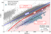 |
Fig. 1 Distribution of molecular (grey dots) and atomic (HI) filaments (grey triangles) in the M–L phase space. Most data are taken from all the public surveys included in Hacar et al. (2023) (and references therein) plus some additional values from Socci et al. (2024a). Superposed to our data, we also display the M-L distribution of ATLASGAL clumps (Urquhart et al. 2018, light blue diamonds; with L = 2 × RAGAL in our notation) and their corresponding power-law fit (dashed black line). HFS are also highlighted in this plot (blue crosses; Table A.1). Overall, most filaments follow a M-L scaling relation such as L ∝ M0.5 (dotted blue line). We indicate the virial line mass mvir for equipartition reported for filaments which separates the subvirial and supervirial regimes (solid red line; Eq. (5)) as well as lines of constant line mass m = [10, 100, 103] M⊙ pc−1 (dotted grey lines). We also include the mass threshold for high-mass star formation MHM = 870 M⊙ ⋅ (Reff /pc)1.33 (dotted purple line; Kauffmann & Pillai 2010), for which we assumed L = 2 × Reff. |
2.2 HFS as precursors of young star clusters
In Fig. 1, we display the position of different HFS reported in the literature and compiled in Appendix A (see Table A.1 and reference therein). The HFS included in our sample show typical masses of MHFS ~ 100−2 × 10⁴ M⊙ and sizes up to LHFS ~ 5 pc. The above observables translate into HFS line masses of  and average surface densities
  as expected for these systems (Myers 2009; Kumar et al. 2020).
The HFS explored in our work populate a parameter space similar to the most massive gas clumps identified in different Galactic surveys (e.g., Urquhart et al. 2014, 2018; Barnes et al. 2021; Elia et al. 2017, 2021; Peretto et al. 2023). In particular, the properties of these HFS mimic those of the most massive ATLASGAL clumps (Urquhart et al. 2014) with median values of MAGAL ~ 2 × 10³ M⊙, RAGAL ~ 0.95 pc, ΣAGAL ~ 4 × 1022 cm−2, and AAGAL ~ 1.38, respectively. Their distribution also roughly follows the same M–L relation (dashed black line) derived for the complete ATLASGAL clump sample (light blue diamonds; Urquhart et al. 2018) as well as from other Galactic Plane clump surveys such as Hi-GAL (not shown; Elia et al. 2021). These similarities suggest that some of these apparently compact clumps might resolve into HFS when observed at high resolution (e.g., see Anderson et al. 2021, for some recent examples). Likewise, most of the HFS compiled in our sample lie above the mass threshold for high-mass star-formation proposed in previous studies (dotted purple line; see Kauffmann & Pillai 2010) which denotes the potential of these regions to form massive stars.
Different studies have proposed a direct connection between HFS and the origin of young star clusters (e.g., Myers 2009; Peretto et al. 2013; Zhou et al. 2022; Kumar et al. 2020). Analogous to the ATLASGAL clumps (see also Urquhart et al. 2014, 2018), our results postulate these HFS as potential gas precursors of typical Milky Way proto-clusters with embedded stellar masses between M⋆ ~ 50–2000 M⊙ (assuming a fiducial star formation efficiency of ϵSF < 10%, i.e. M⋆ ~ ϵSF ⋅ MHFS, in a first order approximation) and thus contain up to a few massive stars (Kroupa & Boily 2002). We note however that different gas conditions may be needed to explain the origin of young massive clusters with M⋆ > 104 M⊙ (see Longmore et al. 2014; Krumholz & McKee 2020, for a discussion).
Remarkably, these HFS (as well as most of the ATLASGAL and Hi-GAL clumps) depart from the scaling relation described by Eq. (1) and show systematically higher total (M) and line (m) masses than regular filaments on scales of ~0.5–5 pc populating the lower right side of the M–L diagram (blue crosses). Also, while most of the ISM filaments can be classified as as subvirial (m < mvir), all HFS appear to be supervirial (m > mvir, beneath the red line) in opposition to filaments with similar masses.
2.3 A toy model to explore the M–L parameter space
We aim to understand and characterize the different locations of filaments and HFS throughout the M–L parameter space. For that, we create a toy model that describes a generalized form of Eq. (1) with different normalization values a. As suggested by Hacar et al. (2023), this normalization value is likely connected to the mean column density of these filaments since denser filaments appear to be on the lower side of this relation. To explore this hypothesis we can estimated the (average) surface density of a filament as
 (6)
(6)
For convenience, and similar to Pon et al. (2012), we also defined the aspect ratio of a filament A = L/FWHM as function of its radius (R = FWHM/2) as
 (7)
(7)
Inserting Eqs. (2) and (7) in Eq. (6), it follows that
 (8)
(8)
which links the observed (average) surface density of filaments with their (typical) aspect ratio.
Coming back to the M–L relation, we can replace Eq. (1) assuming a constant density coefficient b0 in Eq. (2) such as
 (9)
(9)
and combine it with Eq. (7) to express the normalization parameter a by means of aspect ratio A as
 (10)
(10)
Alternatively, by using Eq. (8), this parameter can also be written as
 (11)
(11)
Equations (10) and (11) connect the normalization of the M–L relation in filaments with their (typical) aspect ratio A and average surface density Σ, respectively (an alternative derivation of these equations can be found in Appendix B). In particular, filaments with smaller A, and therefore higher Σ, are expected to follow a M–L relation with a lower normalization value, while filaments with a longer A, and consequently lower Σ, are predicted to exhibit higher normalization values, which cause them to lie higher up in the M–L plane. Spheroidal clouds can be described as the asymptotic limit of filaments when A → 1. Starting from Eq. (6), it is trivial to demonstrate that the classical assumption of spherical symmetry (i.e. 2R = L) leads to clouds with roughly constant Σ (e.g., Larson 1981). Instead, different surface density values are allowed in filaments with varying A > 1 according to Eq. (8), where spheres appear in the asymptotic limit when A →1.
Combined with Eq. (1), Eq. (11) also leads to an additional and direct consequence of our model: the average column density in filaments should scale with their mass and length such as
 (12)
(12)
which is different from the expected correlation for a uniform sphere  . The correlation described by Eq. (12) may be intuitively clear when comparing filaments with the same mass M, where shorter filaments are expected to show higher surface densities. Likewise, filaments of the same length and increasing mass should correspond to higher surface densities.
It is worth emphasizing that the above derivations assume a constant density coefficient, b0 , and a variable normalization parameter, a (see also Appendix B). Inverting these assumptions, that is, having a variable b0 and constant a, would lead to a direct proportionality between the filament surface density and aspect ratio, such as Σ ∝ A (also following the same Eqs. (1) and (6)). This possibility seems to be ruled out given the anticorrelation seen between Σ and L in Fig. 3, which closely follows the predictions of Eq. (12) (see Sect. 2.4 for a full discussion).
Equations (1)–(11) provide an idealized framework to explore the correspondence between the observed mass and length of filaments and HFS and additional physical parameters such as A and Σ. While oversimplified by the use of symmetries and average properties, the next sections will prove this toy model as a useful tool to describe the different physical regimes of the filamentary ISM.
2.4 Comparison with observations
In Fig. 2, we show the corresponding M–L scaling relations expected for aspect ratios A = 3, 10, and 30 (black lines) describing typical values for filamentary geometries obtained combining Eqs. (1) and (10). We also show the corresponding line for A = 1.5 (dashed orange line) characteristic of prolate objects such as HFS (e.g., Kumar et al. 2020). According to these model predictions, standard filaments should present mass and length values corresponding with A > 3 and (average) surface densities of Σ < 8 × 1021 cm−2 (see Eq. (8)). Previous observations reported molecular filaments that show typical A = 5-15 and maximum values of A ~ 30, with corresponding peak surface densities between Σ0 = 8 × 10²⁰−8 × 1021 cm−2 (e.g., Arzoumanian et al. 2019; Schisano et al. 2020). These results are in close agreement with our model5.
In Fig. 3, we directly compare the prediction of Eq. (12) with the filament properties obtained by Schisano et al. (2020) from the analysis of the Herschel Hi-GAL survey (Molinari et al. 2010) which obtained a census of >18 000 filaments across the Galactic Plane. For each filament in this survey, we display the filament average column density Σ and compare it with their corresponding M0.5/L ratio. Figure 3 shows a clear correlation between these observables along more than an order of magnitude in each axis. A linear fit to the Hi-GAL filaments (in log-log space) leads to  for all datapoints (dashed black line) and shows a good agreement (within the noise) with the expected Σ ∝ M0.5/L dependence of our model (dotted red line). A better fit, with
  , can be obtained if we only consider those filaments with Σ > 1021 cm−2, where the Hi-GAL sample is expected to be less affected by completeness (dotted black line; see Schisano et al. 2020, for a discussion of this threshold). A roughly similar dependence (with
  ) has been reported by Schisano et al. (2020) (see their Fig. 26) for these Hi-GAL filaments as well as by Arzoumanian et al. (2019) (see their Fig. 10, panel a) in the case of the Herschel Gould Belt Survey (HGBS) in nearby clouds.
As an additional consequence of Eq. (12), our model predicts a stratified distribution of the ISM filaments in the M–L phase space. In particular, molecular filaments are expected to populate the M–L plane following a similar functional dependence (L = a ⋅ M0.5; Eq. (1)) but with different normalization values, a, depending on their mean column densities (i.e. a ∝ 1 /Σ, as per Eq. (11)). We explored these predictions in Fig. 4 by displaying, once again, the M–L distribution of ISM filaments this time (and when available) color-coding each target by its corresponding average column density Σ (see the color bar). Gaps in this diagram correspond to different observational biases and incompleteness affecting our filament sample (see Hacar et al. 2023, for a discussion). A systematic variation is seen as function of Σ across this plot, where filaments with similar column densities define parallel bands of different colors and where filaments with larger column densities are preferentially located towards the lower side of this distribution (see also Appendix C). When including the unavoidable data noise, the column density values predicted by our model are in good agreement with the observed filament column densities across the entire M–L space.
Likewise, and according to Eqs. (8) and (10), the filament aspect ratio and mean column density should be anti-correlated A ∝ Σ−1 leading to a scaling relation such as L ∝ A ⋅ M0.5. Lines of constant A at different L values would suggest that the filament FWHM is therefore not constant; rather, it may vary significantly when comparing filaments on different scales (L ∝ A ⋅ M0.5 → FWHM ∝ M0.5). We have tested this hypothesis in Fig. 5 by comparing the M–L distribution of those resolved filaments identified by the HGBS (solid triangles; Arzoumanian et al. 2019, ; priv. communication) as well as in different fiber surveys (solid circles; Hacar et al. 2013, 2017b; Socci et al. 2024a) and show them color-coded by their mean column density Σ (left panel) and aspect ratio A (right panel), respectively. Inversely proportional to the previously discussed dependence with Σ (left panel; similar to Fig. 4), these resolved filaments show a tentative stratification as function of A (right panel) with filaments with lower aspect ratios populating the lower part of these diagrams roughly following our model predictions (see legend and color bar). While undoubtedly less systematic, we note that observational, selection, and algorithmic biases between these surveys (see André et al. 2019; Hacar et al. 2023, for relevant discussions) make these A estimates intrinsically noisier than direct Σ measurements. Unfortunately, these comparisons cannot be extended to the Hi-GAL sample given the limited resolution of Herschel to resolve most Galactic filaments at kpc distances. Additional high-resolution data are needed to confirm this predicted FWHM ∝ M0.5 dependence6.
Continuing the above trend, the predicted values from Eq. (10) for A = 3 separate most of the ISM filaments (A > 3)7 from the location of the most massive and compact HFS (A < 34) in Fig. 4. This transition at A = 3 corresponds to regions with Σ = 8 × 1021 cm−2 (Eq. (8); solid black line) and an average density n > 104 cm−3 at scales of ~1 pc (Eq. (2)). The location of the observed HFS coincides with the expected parameter space for spheroids with low aspect ratios A ≤ 1.5 and high column densities Σ > 2 × 1022 cm−2 (dashed orange line), in close agreement with observational results (Myers 2009; Kumar et al. 2020; Morii et al. 2023). Our findings suggest a change of the gas geometry, between filamentary to spheroidal, during the formation of these compact HFS as driver for their formation.
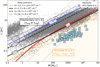 |
Fig. 2 Model predictions (Sect. 2.3) compared to the location of the ISM filaments in the M–L phase space (see also Fig. 1). For simplicity, we display only those molecular filaments. Using Eq. (10), different lines indicate the expected normalization values for characteristic filamentary (A = 30, 10, and 3; black lines) and prolate spheroids (A < 3, orange shaded area) geometries. We added also the typical A observed for HFS (A ≤ 1.5; orange dashed line; e.g., Kumar et al. 2020). We also indicate their corresponding surface densities according to Eq. (11) in the legend. |
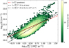 |
Fig. 3 Comparison between the average column density Σ and the M0.5/L ratio observed in the Hi-GAL filaments (> 18 000 filaments; Schisano et al. 2020) displayed using a hexagonal 2D density plot (see color bar). Overplotted on these data, we display the prediction from Eq. (12) (dotted red line) as well as different fits to the data (dashed and dotted black lines; see legend). |
 |
Fig. 4 Mass-Length (M-L) distribution of molecular filaments (circles) similar to Fig. 1, this time color-coded by their average column density Σ (see color bar). The majority of these Σ measurements (> 18 000) were obtained by the Hi-GAL survey (Schisano et al. 2020), while a few additional datapoints (152) have been taken from our Paper III (Socci et al. 2024a). Analogously to Fig. 2, the different lines indicate the predicted distribution of filaments with a mean column density of Σ = [0.8, 2, 8, 16] ⋅ 1021 cm−2 (see legend) according to Eqs. (1) and (11). This corresponds to aspect ratios of A = [30, 10, 3, 1.5], respectively, following Eq. (10). The location of all HFS (grey crosses) are indicated in this plot for comparison. We note that the position of the HFS would correspond with the expected location for prolate (A ≲ 1.5) and high-column density (Σ > 1022 cm−2) structures according to the predictions of our model. See also Fig. C.1. |
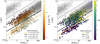 |
Fig. 5 M–L distribution of the nearby HGBS filaments (triangles; Arzoumanian et al. 2019, ; priv. commun.) and fibers (circles Hacar et al. 2023; Socci et al. 2024a,b) color-coded by their mean column density Σ (left panel) and aspect ratio A (right panel). Labels and lines are similar to those in Fig. 4. |
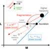 |
Fig. 6 Schematic description of the evolution of sub-critical filaments in the M–L phase space experiencing hierarchical fragmentation. See text for a description. |
3 Evolutionary timescales and accretion rates
3.1 Relevant timescales
The evolution of radially stable filamentary structures (i.e. subvirial or m ≲ mυir) in the M–L plane can be described by the combined effect of three independent processes, each with a specific signature in this parameter space (see top left corner in Fig. 6): (a) fragmentation (splitting an object into pieces of smaller M and L, and thus moving them diagonally downwards in the M–L space); (b) accretion (moving objects horizontally towards higher M at constant L); and (c) longitudinal collapse (moving objects downwards in L at constant M). We can then characterize the relative importance of these three independent processes by comparing their corresponding timescales (see Hacar et al. 2023, for a full discussion).
First, the fragmentation timescale (τf raɡ) is defined as (Larson 1985; Inutsuka & Miyama 1992)
 (13)
(13)
When applying Eq. (2), this can be re-written as8
 (14)
(14)
Second, the accretion timescale (τacc) is defined as the time to double the mass of a filament given an accretion rate ṁ (in units of M⊙ pc−1 Myr−1 ):
 (15)
(15)
A connection between the filament line mass m = M/L and the gas accretion rate ṁ may be expected if accretion would be gravitationally driven (e.g., Heitsch 2013), although we remark that this condition is not imposed in our model. Instead, our generic definition of τacc aims to describe the timescale in which accretion has a noticeable influence in the filament gas dynamics irrespective of its nature (e.g., turbulent accretion; see Padoan et al. 2020).
Third, the timescale for longitudinal collapse (τlonɡ), or the time for collapse along the main filament axis, can be described as a function of the free-fall time  as (Pon et al. 2012; Toalá et al. 2012; Hoemann et al. 2023)
 (16)
(16)
The combination of Eqs. (13) and (16) to eliminate the density dependence gives
 (17)
(17)
which demonstrates that the time for longitudinal collapse τlonɡ of filaments (A > 3) is longer than the fragmentation timescale (i.e. τlonɡ >> τ f raɡ) and therefore is dynamically subdominant in elongated geometries (see also Pon et al. 2012; Toalá et al. 2012).
3.2 Low accretion rates in filaments
Following Sect. 3.1, the distribution of filaments in the M–L phase space is determined by the competition between fragmentation and accretion processes (A > 3 → τlonɡ ≫ τfraɡ ∼ τacc). We illustrate these results in Fig. 6 (see also Hacar et al. 2023, for a full discussion). At any point of its hierarchy, a filament of mass M and length L (higher hierarchy level) will fragment into several sub-structures of lower M and shorter L (lower hierarchy level) in a timescale τfraɡ (Eq. (14)). Driven by a fast turbulent fragmentation, the connection between two hierarchical levels is expected to statistically follow a random-walk realization such as L ∝ M0.5 (similar to Eq. (1)) with a normalization value determined by the higher level of this hierarchy (dashed red line). Simultaneously, each sub-structure is expected to accrete mass from their surroundings at a rate given by their local ṁ increasing its mass by a factor of two in a timescale τacc (Eq. (15)). This mass gain (black arrow) can continue a maximum timescale comparable to τacc ≥ τfraɡ (solid blue line) in which this structure is expected to fragment again into a lower hierarchy level. This balance can be estimated equating Eqs. (14) and (15):
 (18)
(18)
Our model therefore predicts the location of hierarchical filaments in the M–L phase space to be bracketed between the correlations defined by Eq. (1) (upper bound) and Eq. (18) (lower bound).
Equation (18) defines a power-law relationship in the M–L diagram (see Fig. 6), crossing this plot from its lower left to the upper right, with lower normalization values for higher accretion rates, ṁ. This can be seen after re-arranging Eq. (18) as follows:
 (19)
(19)
demonstrating how M and m appear to be good proxies of ṁ according to our model. A similar correlation between ṁ and m has been recently found in simulations, which suggests that the line mass of filaments is largely determined by their accretion rates (Feng et al. 2024; Zhao et al. 2024).
We display some characteristic values of ṁ predicted using Eq. (18) in the M–L diagram in Fig. 7 (solid lines; see also color bar). In agreement to our model predictions, observations in nearby filaments report accretion rates ṁ ~ 10– 30 M⊙ pc−1 Myr−1 (e.g., Palmeirim et al. 2013; Bonne et al. 2020), with higher accretion rates of ṁ ≤ 100 M⊙ pc−1 Myr−1 typically associated with star-forming filaments according to Galactic Plane surveys (Schisano et al. 2014). Our model satisfactorily reproduces the specific M and L distributions of hierarchical filaments in regions such as Musca, Taurus, and Orion (see Fig. 9 in Hacar et al. 2023). The relatively low range of accretion rates ṁ ~ 10 – 100 M⊙ pc−1 Myr−1 found in filaments explains how these structures show a similar and continuous M–L relation across several orders of magnitude in mass and length.
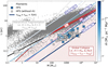 |
Fig. 7 Μ–L plot similar to Fig. 1, this time showing curves where τfraɡ = τacc for different accretion rates, namely ṁ = [10,100,103,104] M⊙ pc−1 Myr−1 (straight blue lines), using different colors (see individual labels and color bar). We display those HFS with accretion measurements using the same color-code (see color bar on the right). We highlight the region with expected global (radial + longitudinal) collapse (shaded brown area; where τlonɡ ~ τff ~ τfraɡ) corresponding to the area where both spheroidal (A ≤ 3; black line) and supervirial (m > mυir; red curve) conditions are satisfied (see also Fig. 2). |
3.3 High accretion rates in HFS
The different locations of filaments and HFS in the M–L phase space translate into different accretion rates ṁ according to Eq. (18). As seen in Fig. 7, HFS are consistent with accretion rates of ṁ ≳ 200–300 M⊙ pc−1 Myr−1, that is much higher than those expected for most ISM filaments (Sect. 3.2).
Previous observational works have independently investigated the total accretion rate in HFS using mass flows along filaments feeding the HFS (e.g., Kirk et al. 2013; Peretto et al. 2013; Hacar et al. 2017a; Williams et al. 2018) and/or infall motions along the line of sight associated with the gas around these objects (e.g., Walsh et al. 2006; Schneider et al. 2011; Yang et al. 2023). We have compiled some of these studies in Table A.1 (see references therein)9. Accretion rates in HFS are estimated to be in the range between ṀHFS ~ 20–4500 M⊙ Myr−1 with a mean value of ṀHFS ~ 1000 M⊙ Myr−1. For comparison, the typical accretion rates onto dense cores at scales of ∼0.1 pc is estimated between Ṁ ~ 10 M⊙ Myr−1 (Lee et al. 2001) and Ṁ ~ 100 M⊙ Myr−1 (Wells et al. 2024).
We find a direct correlation between the observed HFS masses MHFS and their corresponding accretion rates ṀHFS . We illustrate this correlation in Fig. 8 (upper panel) where a fit to these data retrieves an almost linear proportionality between these quantities following  (red dashed line). The above correlation is steeper than the one found for massive clumps (Traficante et al. 2023; Zhou et al. 2024) and cores (Wells et al. 2024).
We converted the above ṀHFS values into equivalent accretion rates per unit length ṁHFS assuming ṁHFS = ṀHFS /LHFS. In Fig. 7, we color-coded the above the estimated rates ṁHFS similar to our model predictions (see color bar). As expected, observations report accretion rates between ṁHFS ≳ 50–2000 M⊙ pc−1 Myr−1 in HFS of M > 100 M⊙.
We further illustrate the relative good agreement between these estimates in Fig. 8 (lower panel) where we display the individual observed mass accretion rates ṁHFS against the corresponding predictions for ṁpred from Eq. (19) given the MHFS and LHFS values in Table A.1. We note that the predictions derived from Eq. (19) only assume that the accretion timescale is equal to the fragmentation timescale (Eq. (18)) as working hypothesis of our toy model (Sect. 2). We observed a positive correlation between ṁHFS and ṁpred (dashed grey line;  ), although our model seems to slightly overpredict the actual accretion rates by a factor of ∼3. Similarly to Fig. 8 (upper panel), a comparison between the observed mHFS and ṁHFS (not shown) also retrieves a positive and tight correlation between these observables close to our expectations where
  (albeit again with some scatter). The obvious limitations of our toy model together with observational biases such as projection effects and large uncertainties on the mass estimates can hamper these comparisons. Given its simplicity and basic assumptions, however, this close correspondence between these observed and predicted accretion rates reinforces the validity of these estimates, at least in a first-order approximation.
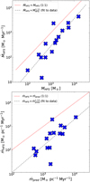 |
Fig. 8 Accretion rates in HFS. Upper panel: comparison between observed total accretion rates (ṀHFS) and the HFS mass (MHFS) reported in the literature for HFS (see also Table A.1). Lower panel: comparison between observed accretion rates per-unit-length (ṁHFS) and those predicted following Eq. (19) (ṁpred). A red dotted line shows the expected 1:1 correlation between these values. A grey dashed line indicates a fit to the data (in log-log space) in both panels (see legend). |
4 Inducing gravitational collapse
4.1 A geometric phase-transition
Mergers and collisions between filaments (Duarte-Cabral et al. 2011; Nakamura et al. 2014; Jiménez-Serra et al. 2014; Beltrán et al. 2022; Kumar et al. 2022) and more generally converging flows (Heitsch et al. 2008; Schneider et al. 2010; Galván-Madrid et al. 2010) and cloud-cloud collisions (Higuchi et al. 2010; Fukui et al. 2014; Wang et al. 2022; Zhou et al. 2023), have been suggested as the potential origin of parsec-size HFS leading to the formation of clusters in the Solar neighborhood (Nakamura et al. 2012; Duarte-Cabral et al. 2010), massive IRDCs (Schneider et al. 2010; Galván-Madrid et al. 2013; Panja et al. 2023), as well as superclusters in both the Milky Way (Fukui et al. 2016) and the Magellanic Clouds (Fukui et al. 2015; Saigo et al. 2017). Different kinematic (Duarte-Cabral et al. 2011; Torii et al. 2017; Haworth et al. 2015) and chemical (Jiménez-Serra et al. 2010; Sanhueza et al. 2013) features have been proposed as observational signatures of these collisions. Kinematic studies reveal clear signatures of global inward motions as signature of the gravitational collapse of these HFS after formation (Myers 2009; Peretto et al. 2013; Hacar et al. 2017a; Williams et al. 2018; He et al. 2023; Zhou et al. 2024; Zhang et al. 2024). As expected for gravitationally dominated systems, magnetic fields appear to be sub-dominant in HFS once their collapse has started (Pattle et al. 2017; Wang et al. 2020; Arzoumanian et al. 2021). Alongside these works, our toy model provides a simple and testable analytic framework aiming to capture the main physical properties of these HFS.
Compared to filaments, and according to Eq. (17), τlonɡ becomes comparable to τfraɡ in more prolate geometries ( A < 3; Pon et al. 2012; Toalá et al. 2012) and should therefore be considered for their evolution (τlonɡ < τfraɡ). For regions where also m > mvir (i.e. supervirial) the radial collapse timescale (τcol ~ τff) becomes comparable to the fragmentation timescale (τcol ~ τfraɡ; e.g., Inutsuka & Miyama 1997). Filamentary clouds located towards the right, lower corner of Fig. 7 simultaneously satisfy both conditions, namely, they are spheroidal with A ≲ 3 and are supervirial with m > mυir. They are therefore prone to collapse. This transition from a filamentary (A > 3) to a spheroidal (A ≲ 3) geometry can therefore induce the global (longitudinal + radial) collapse of a object since in these regions all timescales are comparably fast, i.e. τlonɡ ~ τfraɡ ~ τcol. We have indicated the parameter space for this (gravitational) global collapse in Fig. 7 (shaded brown area) defined as the area where both spheroidal and supervirial conditions are satisfied (see also Fig. 2).
A geometric phase-transition between a filamentary and a spheroidal (A = 3) configuration could explain the origin of HFS. As shown in Fig. 7, HFS are identified as supervirial structures (m > mυir) with sphere-like aspect ratios ( A < 3), displaying high mass accretion rates (ṁ > 300 M⊙ pc−1 Myr−1, Sect. 3.3). Unlike filaments, these objects satisfy the conditions for global collapse on scales of 0.5–2 pc in timescales of ~ 1 Myr (see above). We notice that, although it is not required by our analytic calculations, the transition into collapse at A ≤ 3 occurs at an average surface density of Σ ≥ 8 × 1021 cm−2 (or AV ~ 8 mag), which is coincident with the threshold for star formation observed in nearby clouds (Lada et al. 2010).
The notion of induced gravitational collapse after merging (see models and references above) is reinforced by the comparison between the properties of the HFS and their individual filaments. In Fig. 9, we display those regions in our sample for which mass and length measurements of their connecting, pc- scale filaments are available (color coded, see legend; see also references in Table A.1). As discussed in Sect. 2.3, the predicted line for A = 3 separates these (sub)virial filamentary structures from their supervirial HFS also in individual targets. In all cases the local line mass (see dotted black lines) of the HFS (mHFS) is also more than three times higher than the corresponding line mass of any of their individual filaments mf , even in extreme cases such as DR21 (Schneider et al. 2011; Hennemann et al. 2012) or Mon-R2 (Treviño-Morales et al. 2019; Rayner et al. 2017). As discussed by Hacar et al. (2023), the segmentation of a filament would preserve its line mass leading to changes along constant m values and consequently mHFS ~ mf,i. On the contrary, correlations such as mHFS > mf,i indicate that HFS locally (≲1 pc) gathered additional mass via merging of filaments (e.g. mHFS,0 ~ ∑imf,i); this, in turn, triggers high accretion rates (Sect. 3.3) due to the induced gravitational collapse of these supervirial regions.
The observed HFS mass MHFS is expected to combine the contributions of the initial HFS mass MHFS ,0 and the mass accreted over time τ such as MHFS (τ) = MHFS,0 + M ⋅ τ or, similarly, mHFS (τ) = mHFS ,0 + ṁHFS ⋅ τ, if written in terms of line mass. In a simplified configuration in which a newly formed HFS condenses all the mass of the merger, so mHFS,0 ~ ∑imf,i, the line mass of a HFS over time could be described as
 (20)
(20)
The final value of mHFS can be further amplified by the collapse of these regions reducing L. The results shown in Fig. 9, where several targets show mHFS > ∑imf,i, suggest that the currently observed mass accretion rates after merging ṁHFS (Sect. 3.3) could significantly contribute to the mass of these regions within the typical evolutionary times for HFS of τ ~ 1–2 Myr (Myers 2009).
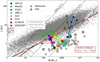 |
Fig. 9 M–L plot comparing those HFS (crosses) with their pc-scale filaments (circles). Individual regions, where filaments and HFS are connected by segments, are color coded in the plot (see legend; see references in Table A.1). Lines and labels are similar to Fig. 7. We highlight different diagonal lines defining individual m = M/L values (=[10,100,100] M⊙ pc−1; dotted black lines). |
4.2 Filamentary vs spherical accretion
Increasing observational evidence demonstrates the presence of significant filamentary accretion flows onto HFS (e.g., Kirk et al. 2013; Chen et al. 2019; Baug et al. 2018; Dewangan et al. 2020; Ma et al. 2023; Panja et al. 2023; Rawat et al. 2024). These findings have led to the proposal of formation scenarios for high- mass stars involving multiple-scale processes in HFS such as the clump-fed (Tigé et al. 2017; Motte et al. 2018; Peretto et al. 2020) and the inertial-inflow models (Padoan et al. 2020).
Following a simplified merging scenario (Sect. 4.1), our description assumes that most of the mass in a HFS can be originally associated with filamentary structures at larger scales. Different CO surveys included in our HFS sample such as G326 (He et al. 2023), G323.46 (Ma et al. 2023), G6.55 (Sen et al. 2024), or G148.24 (Rawat et al. 2024), as well as other studies targeting HFS (Anderson et al. 2021; Peretto et al. 2023), appear to support this working hypothesis. However, the actual gas organization inside and outside HFS is likely more complex. The gas in molecular clouds is known to be multi-fractal and combines diffuse (Gaussian) and filamentary (non-Gaussian) contributions at all scales (Robitaille et al. 2020). HFS may thus accrete material from both filaments and diffuse gas simultaneously.
The distinction between these collimated (filamentary) and spherical (diffuse gas) accretion modes in HFS is customary in other astrophysical problems such as the study anisotropic accretion onto galaxies via cold streamers (e.g., Dekel et al. 2009). The relative importance of these two accretion modes can be evaluated using geometrical considerations. The total mass accretion Ṁ can be parameterized from the gas mass flux over the solid angle Ω produced by gas at a density n with an accretion velocity, υacc, such as Ṁ = n ⋅ Ω ⋅ υacc (e.g., Kirk et al. 2013; Peretto et al. 2013; Hu et al. 2021). At a radius, r, from the center of a HFS, the total filamentary accretion funnelled by Nf filaments of radius Rf, cross section  , and density nf, over a solid angle
  is then
 (21)
(21)
On the other hand, the maximum spherical accretion produced by the background gas of density nbɡ outside filaments can be estimated as
 (22)
(22)
Assuming that both gas components experience the same accretion velocity υacc (e.g., free-fall), the relative contribution of these filamentary and spherical accretions to the evolution of the HFS can be evaluated as
 (23)
(23)
To be dynamically relevant (i.e. Ṁbɡ ~ Ṁf), the density of the diffuse gas around the HFS must be
 (24)
(24)
Using Eq. (24), it is easy to demonstrate that at the short radii r ≲ 2Rf (~RHFS ) expected at the intersection of Nf = 2 filaments, the density of the diffuse gas needs to be comparable to the gas density in filaments (nbɡ > nf /7) to influence the mass growth of HFS. This background density should be even higher if more filaments Nf > 2 contribute to the filamentary inflow. On the other hand, diffuse accretion may become more relevant at larger radii outside the central HFS where the minimum density contrast required by Eq. (24) decreases rapidly via  at r >> Rf .
As discussed in Sect. 3.2, diffuse gas accretion determines the evolution and mass load of individual filaments. On the contrary, the accretion of diffuse gas onto HFS may play a secondary role with respect to the mass accreted throughout filaments (Ṁf > Ṁbɡ) unless embedded in a high density environment. Given the high column density contrast seen in HFS (Myers 2009; Kumar et al. 2020), mass accretion in HFS is then expected to be dominated by filamentary flows, in agreement to simulations (Gómez & Vázquez-Semadeni 2014; Vázquez-Semadeni et al. 2019).
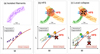 |
Fig. 10 Illustrative cartoon describing the configuration (top panels) and location of filaments and HFS in the M–L phase space (bottom panels). From left to right: (a) hierarchical fragmentation of isolated filaments (circles) into sub-filaments (triangles); (b) formation of a HFS system at the intersection of multiple filaments; and (c) local gravitational collapse of the resulting parsec-scale clump. Black arrows indicate how this collapse may lead into the shrink of both the central clump and subfilaments in the HFS moving these objects downwards in the M–L phase space. Similarly to Fig. 8, a brown line in these plots indicates the transition between hierarchical fragmentation (above the line) and global collapse (beneath the line). |
4.3 A dichotomy in the M–L phase space
In addition to previous formation models (see Sect. 4.1), we aim to explain how HFS may evolve outside the main sequence of filaments seen in the M–L plane generated by their turbulent fragmentation (Sect. 3.2) and populate a different regime of this phase space (see Fig. 1). To facilitate our description, we summarize these differences in three characteristic configurations shown by corresponding cartoons in Fig. 10 motivated by our previous observational results and models (Figs. 7–9). These diagrams are made for illustrative purposes only, acknowledging the strong (over)simplifications of these cartoons. Detailed simulations are needed to explore more realistic, self-consistent evolutionary tracks for different filament and HFS configurations (e.g., Feng et al. 2024).
Multiple mechanisms generate parsec-size, elongated (A >> 3) structures as part of the intrinsic filamentary nature of the ISM (see Hacar et al. 2023, and references therein). Usually showing a low column density (Σf ) and subvirial state (mf < mυir), these parsec-size filaments (circles) typically fragment creating a hierarchical sub-structure of smaller filaments (triangles) that move diagonally towards the lower left corner of this M–L diagram, following a relation such as L ∝ M0.5, as described by Eq. (1) (Fig. 10, panel a; see also Sect. 3.2 and Fig. 6). Given their relatively low accretion rates ṁ ~ 10–100 M⊙ pc−1 Myr−1, isolated filaments are therefore unable to reach the conditions for the formation of high-mass stars.
On the other hand, HFS are created at the junction of several of these parsec-size filaments (Fig. 10, panel b). With typical cross sections of ∼1 pc, these filament junctions generate prolate regions (A ≤ 3), which rapidly increase both the total (MHFS ) and line (mHFS > mf ) masses as well as the clump surface density (ΣHFS > Σf). This shifts the HFS towards the lower right direction in the M–L diagram with respect to their initial filaments (mHFS > mf ), as shown in Fig. 9.
If the merging of filaments is efficient enough, the high accretion rates ṁ ≳ 300 M⊙ pc−1 Myr−1 in these junctions (Sect. 3.3) could make them locally supervirial (mHFS > mυir). The resulting HFS would then collapse by its own gravity (τfraɡ ~ τlonɡ; Sect. 4). Upon shrinking in size and gaining mass (while also fragmenting inside, triangles to the left), this runaway process may continue moving the HFS downwards in the M–L phase space, away from the main distribution of filaments (Fig. 10, panel c). This global collapse may explain the apparent gap between HFS and filaments in the M–L phase space. Other gas structures inside these HFS (e.g., cores and sub-filaments) would likely experience additional compression induced by the parsec-scale collapse (moving down in this M–L diagram). Unlike any filament fragmentation process (where mf < mυir), the collapse induced during the transition from elongated to prolate geometries marks a physical change (phase-transition) on the evolution of these HFS and the only way to agglomerate enough mass to form large stellar clusters (M⋆ > 100 M⊙), and eventually high-mass stars, in timescales of ≲1 Myr (Motte et al. 2018).
Panels b and c in Fig. 10 resemble the early stages I plus II proposed by Kumar et al. (2020) for the evolution of HFS. In addition to this previous qualitative description, our model provides the physical foundations for some of the early steps on the evolution of HFS as well as direct quantitative predictions for future observations (i.e., M, L, A, Σ, and ṁ). Our analytic description (Sect. 2) also suggests a dichotomy between the dominant physical mechanisms governing the evolution isolated filaments and HFS. Individual, parsec-size filaments primarily evolve in a top-down manner (Sect. 3.2) dominated by an internal turbulent fragmentation ( fray and fragment model; Tafalla & Hacar 2015) populating the main diagonal of the M–L phase space (Fig. 10, panel a). On the other hand, HFS might only emerge from a fast, bottom-up process triggered by the agglomeration of filaments (Sect. 4) and the gravitational collapse of these regions on parsec scales ( gather and fray model; Smith et al. 2016) (Fig. 10, panels b and c).
In models of global hierarchical collapse (e.g., Vázquez- Semadeni et al. 2019; Camacho et al. 2023), HFS appear as the manifestation of a fast local collapse within a much slower large-scale contraction of gravitationally bound clouds. A multiscale organization of HFS including gas flows from cloud to core scales has been proposed to explain the origin of these systems in different high-mass star-forming regions (Zhou et al. 2023; Zhou & Davis 2024). Instead, the observed separation in the M– L phase space appears to not only separate the HFS from their parental filaments, but it suggests that only the former may satisfy the supercritical conditions (m > mυir) for local collapse. Restricted to a volume comparable to the initial merger crosssection, the gravitational collapse in HFS is likely to be limited to a few parsecs within the lifetime of this structures. Our analysis supports recent results indicating that the gas clumps leading to the formation of clusters, analogously to our HFS (Sect. 2.2), may be dynamically decoupled from their molecular clouds at scales of few parsecs (Peretto et al. 2023). The transition to global collapse corresponds with a change on the virial properties (αυir < 1) of these clumps observed at Σ ~ 300 M⊙ cm−2 (or Σ ~ 1.4 × 1022 cm−2) (Kauffmann et al. 2013; Traficante et al. 2020; Peretto et al. 2023) in close agreement with our analytic predictions for HFS with A = 1.5 and Σ ~ 1.6 × 1022 cm−2 (see Eq. (11) and Fig. 2). Our results favor the ideas introduced by the inertial-inflow model for star formation (Padoan et al. 2020), applied here to parsec-size, cluster-forming HFS.
5 Possible scale-free process
Given the fractal, scale-free nature of the filamentary ISM (Falgarone et al. 1991; Elmegreen & Falgarone 1996; Hacar et al. 2023), it would be interesting to explore whether the same transition between filamentary and spherical geometries could also explain the formation of distinct collapsing regions at different scales. High-resolution observations report the existence of hub-like structures created by the interaction of small filaments (aka fibers) at sub-parsec scales in regions such as SDC335- MM1 (Peretto et al. 2013; Xu et al. 2023), NGC 1333 IRAS 3 (Hacar et al. 2017b), G035.39 (Henshaw et al. 2014), OMC-1 Ridge and OMC-2 FIR-4 (Hacar et al. 2018), and OMC-3 MM7 in Orion (Ren et al. 2021), which currently comprise the most massive protostars in these clouds. Translated to smaller masses of M ≲ 100 M⊙, the same physical mechanism operating in the parsec-scale HFS discussed above could also explain the origin of overdensities on subparsec scales if these (mini)hubs would become gravitationally unstable (by entering the shaded area in Fig. 7).
Particularly relevant for this discussion is the origin of high-mass cores (M ~ 10–100 M⊙). Theoretical considerations derive mass accretion rates onto massive stars of Ṁ⋆ = 1– 6 × 10⁻⁴ M⊙ yr−1 (McKee & Tan 2002), consistent with the infall values derived for their parental star-forming clumps at scales of ~0.1 pc (Fuller et al. 2005), that is, ṁ ~ 1– 6 × 10³ M⊙ pc−1 Myr−1. As shown in Fig. 7, the line ṁ = 103 M⊙ pc−1 Myr−1 almost coincides with the relation defining the mass threshold for high-mass star formation with MHM = 870 M⊙ ⋅ (Reff /pc)1.33 (dashed purple line; Kauffmann & Pillai 2010) and similar revised estimates (MHM = 1282 M⊙· (Reff /pc)1.42; Baldeschi et al. 2017). In analogy to the large HFS, the merging of filaments at sub-parsec scales inducing junctions (or forks) with masses below this line could trigger the formation of such massive cores, a possibility currently explored in simulations (Smith et al. 2011; Clarke et al. 2017; Hoemann et al. 2021; Kashiwagi et al. 2023; Hoemann et al. 2024). While locally collapsing, these massive cores could still fragment and form a binary (multiple) star system at smaller scales.
Continuing towards lower masses, the process could also be extended to dense (solar-like) cores with typical sizes of L~ 0.1 pc and masses M ~ 3 M⊙ (Myers 1983). Formed out of the quasi-static fragmentation of some of sub-pc filaments at the end of the turbulent cascade (Hacar & Tafalla 2011), the change in geometry from filamentary into a prolate structure (with A = 1.5, see dashed orange line in Fig. 2; Myers et al. 1991) could trigger local collapse in dense cores if τlonɡ ~ τcol (e.g., Heigl et al. 2016). A comparison between our models and the average mass and length properties (M ~ 4.1 M⊙ and L~ 0.12 pc; Myers 1983) as well as accretion rates in dense cores (Ṁ > 10 M⊙ Myr−1 or ṁ > 100 M⊙ pc−1 Myr−1, Lee et al. 2001) appear to support this hypothesis.
The lower mass end of the area defining global collapse is shaped by the sonic (thermal) limit expressed in Eq. ((5)), when  . Low-mass (<2 M⊙) spheroidal ( A < 3) structures could therefore exist without necessarily collapsing (see lower left corner of the M–L phase space). This could explain the existence of small, pressure-confined but still starless cores reported in different star-forming regions (Lada et al. 2008; Kirk et al. 2017). In this low-mass regime, comparatively lower L values (i.e. increasingly higher densities following Eq. (2)) are needed to trigger collapse as expected by the Jeans criterion (MJ ∝ n−1/2). Further observational and theoretical studies are needed to explore the alluring ideas presented in this section.
6 Conclusions
In this paper (Paper V), we introduce an analytic formulation to explore the origin and early evolution of hub-filament systems (HFS) within of the filamentary structure of the ISM. The results of our work can be summarized below:
We investigated the properties of HFS with masses MHFS ~ 100−2 × 10⁴ M⊙ and sizes up to LHFS ~ 5 pc as likely precursors of typical Milky Way clusters with up to a few thousand solar masses in stars (Sect. 2);
The enhanced mass in HFS set these objects apart from the fundamental M–L scaling relation (L ∝ M0.5) governing the filamentary structure of the ISM at similar scales;
Using a simple analytic formulation, we created a toy model to explore the evolution of different filamentary structures in the M–L phase space. Despite its simplicity, our toy model provides direct predictions of the filament aspect ratio (A), average gas column density (Σ), relevant timescales (i.e., τcol, τlonɡ, τfraɡ, τacc), and accretion rates (ṁ). These predictions are in close agreement with observations;
Our model predicts an inverse proportionality between the aspect ratio A and total gas surface density Σ of filaments at different scales. Once fixed, the value of A (or Σ) determines the normalization value a for their expected L = a ⋅ M0.5 correlation;
Most of the molecular filaments in the ISM are bracketed between the model predictions for A ≤ 30 (or Σ = 8 × 1020 cm−2) and A ≥ 3 (or Σ = 8 × 1021 cm−2). On the other hand, HFS occupy the expected parameter space for A < 1.5 (or Σ > 1.6 × 1022 cm−2). Our results suggests that the observed differences between filaments and HFS may arise from the spheroidal geometry of these later objects;
Our model predicts a dichotomy between the dominant physical mechanisms governing the evolution of isolated filaments and HFS (Sect. 3). Filamentary structures with large aspect ratios (A > 3) fragment in timescales much shorter than their longitudinal contraction (τfraɡ < τlonɡ). In contrast, the combination of high line masses (m > mυir) and spheroidal shapes ( A < 3) seen in HFS makes these structures prone to global (radially + longitudinally) collapse (τfraɡ ~ τlonɡ ~ τcol) on timescales of ~ 1 Myr (Sect. 3);
Our analytic calculations predict the fast evolution of HFS to be favored by the high accretion rates (ṁ ≳ 300 M⊙ pc−1 Myr−1) originated at the junction of multiple parsec-scale filaments. Despite its simplicity, our model predictions reproduce the observed variations of Ṁ across more than an order of magnitude in M in HFS;
The change from a filamentary into spheroidal gas organization may induce geometrical phase-transition triggering the (global) gravitational collapse of the HFS at parsec scales (Sect. 4). This transition seems to occur at column densities of Σ ~ 8 × 1021 cm−2, coincident with the previously proposed threshold for star formation;
This gravitational collapse would make these HFS to shrink in size detaching these objects from most ISM filaments in the M–L phase space. Thus, the initial conditions for the formation of high-mass stars and clusters would be set;
We speculate that a similar process might also operate at sub-parsec scales, explaining the formation of similar minihubs and cores connected to the formation of individual stars (Sect. 5).
The geometric phase transition indicated by these results and summarized by our toy model suggests that the origin of clusters may arise as an emergent phenomenon within the filamentary structure of the ISM. Additional systematic surveys of both filaments and HFS, including homogeneous measurements of M, L, A, Σ, Ṁ and ṁ, are needed to confirm these promising results.
Acknowledgements
The authors thank D. Arzoumanian for kindly sharing their data for this analysis. A.H., F.B., and A.S. received funding from the European Research Council (ERC) under the European Union’s Horizon 2020 research and innovation programme (Grant agreement no. 851435). D.S. acknowledges support of the Bonn-Cologne Graduate School, which is funded through the German Excellence Initiative as well as funding by the Deutsche Forschungs- gemeinschaft (DFG) via the Collaborative Research Center SFB 1601 “Habitats of massive stars across cosmic time” (subprojects B4 and B6). Furthermore, the project is receiving funding from the programme “Profilbildung 2020”, an initiative of the Ministry of Culture and Science of the State of Northrhine Westphalia. E.S. acknowledge financial support from European Research Council via the Horizon 2020 Framework Programme ERC Synergy “ECOGAL” Project GA-855130. This work made use of Astropy:10 a community-developed core Python package and an ecosystem of tools and resources for astronomy (Astropy Collaboration 2013, 2018, 2022). This work made intensive use of the python packages Matplotlib (Hunter 2007) and Numpy (Harris et al. 2020).
Appendix A Literature results
The mass (M), length (L), and mass accretion rate (ṁ) for those parsec-scale HFS available in the literature are reported in Table A.1.
Hub-Filament Systems (HFS) at parsec scales: Literature results ordered by mass.
Appendix B Alternative derivation
Equations 8-11 can be also derived from the expected correlation between mass and density with in gas surface density in connection with different scaling relations. In particular, Eq. 6 can be rewritten as
 (B.1)
(B.1)
where in order to fulfil Eq. 1 it requires that
 (B.2)
(B.2)
On the other hand, the average density can be recalculated as
 (B.3)
(B.3)
which again – to satisfy Eq. 2 – necessitates that
 (B.4)
(B.4)
which can be also reordered to get Eq. 8. Introducing Eq. B.4 into Eq. B.2 leads back to Eq. 10 or Eq. 11 depending whether Σ or A is replaced.
Appendix C Observational data
The large number of datapoints (> 20 000 filaments) hampers the visualization of the Σ variations in Fig. 4. In addition to this figure in the main text, in Fig. C.1 we show the different groups of filaments displayed in four ranges of average column density (Σ) similar to those defined by our models (see legend). We note that each of these groups populates a different part of the M–L phase space depending on their corresponding Σ following the predictions of our models (Sect. 2).
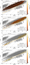 |
Fig. C.1 Same as Fig. 4 but where we display different filament populations grouped in four ranges of average column density (Σ) similar to our models (see also legend). From top to bottom: (a) Σ < 2 × 1021 cm−2, (b) 2 × 1021 cm−2 ≤ Σ < 8 × 1021 cm−2, (c) 8 × 1021 cm−2 ≤ Σ < 1.6 × 1022 cm−2, and (d) Σ > 1.6 × 1022 cm−2. |
References
- Álvarez-Gutiérrez, R. H., Stutz, A. M., Sandoval-Garrido, N., et al. 2024, A&A, 689, A74 [NASA ADS] [CrossRef] [EDP Sciences] [Google Scholar]
- Anderson, M., Peretto, N., Ragan, S. E., et al. 2021, MNRAS, 508, 2964 [NASA ADS] [CrossRef] [Google Scholar]
- André, P., Di Francesco, J., Ward-Thompson, D., et al. 2014, in Protostars and Planets VI, eds. H. Beuther, R. S. Klessen, C. P. Dullemond, & T. Henning, 27 [Google Scholar]
- André, P., Arzoumanian, D., Könyves, V., Shimajiri, Y., & Palmeirim, P. 2019, A&A, 629, L4 [Google Scholar]
- André, P. J., Palmeirim, P., & Arzoumanian, D. 2022, A&A, 667, L1 [CrossRef] [EDP Sciences] [Google Scholar]
- Arzoumanian, D., André, P., Könyves, V., et al. 2019, A&A, 621, A42 [NASA ADS] [CrossRef] [EDP Sciences] [Google Scholar]
- Arzoumanian, D., Furuya, R. S., Hasegawa, T., et al. 2021, A&A, 647, A78 [NASA ADS] [CrossRef] [EDP Sciences] [Google Scholar]
- Astropy Collaboration (Robitaille, T. P., et al.) 2013, A&A, 558, A33 [NASA ADS] [CrossRef] [EDP Sciences] [Google Scholar]
- Astropy Collaboration (Price-Whelan, A. M., et al.) 2018, AJ, 156, 123 [Google Scholar]
- Astropy Collaboration (Price-Whelan, A. M., et al.) 2022, ApJ, 935, 167 [NASA ADS] [CrossRef] [Google Scholar]
- Baldeschi, A., Elia, D., Molinari, S., et al. 2017, MNRAS, 466, 3682 [NASA ADS] [CrossRef] [Google Scholar]
- Ballesteros-Paredes, J. 2006, MNRAS, 372, 443 [NASA ADS] [CrossRef] [Google Scholar]
- Barnard, E. E. 1907, ApJ, 25, 218 [NASA ADS] [CrossRef] [Google Scholar]
- Barnes, A. T., Henshaw, J. D., Fontani, F., et al. 2021, MNRAS, 503, 4601 [CrossRef] [Google Scholar]
- Baug, T., Dewangan, L. K., Ojha, D. K., et al. 2018, ApJ, 852, 119 [NASA ADS] [CrossRef] [Google Scholar]
- Beltrán, M. T., Rivilla, V. M., Kumar, M. S. N., Cesaroni, R., & Galli, D. 2022, A&A, 660, L4 [NASA ADS] [CrossRef] [EDP Sciences] [Google Scholar]
- Bonanomi, F., Hacar, A., Socci, A., Petry, D., & Suri, S. 2024, A&A, 688, A30 [NASA ADS] [CrossRef] [EDP Sciences] [Google Scholar]
- Bonne, L., Bontemps, S., Schneider, N., et al. 2020, A&A, 644, A27 [EDP Sciences] [Google Scholar]
- Busquet, G., Zhang, Q., Palau, A., et al. 2013, ApJ, 764, L26 [NASA ADS] [CrossRef] [Google Scholar]
- Camacho, V., Vázquez-Semadeni, E., Palau, A., & Zamora-Avilés, M. 2023, MNRAS, 523, 3376 [NASA ADS] [CrossRef] [Google Scholar]
- Cao, Y., Qiu, K., Zhang, Q., & Li, G.-X. 2022, ApJ, 927, 106 [NASA ADS] [CrossRef] [Google Scholar]
- Chen, H.-R. V., Zhang, Q., Wright, M. C. H., et al. 2019, ApJ, 875, 24 [Google Scholar]
- Chung, E. J., Lee, C. W., Kim, S., et al. 2021, ApJ, 919, 3 [NASA ADS] [CrossRef] [Google Scholar]
- Clarke, S. D., Whitworth, A. P., Duarte-Cabral, A., & Hubber, D. A. 2017, MNRAS, 468, 2489 [Google Scholar]
- Dekel, A., Birnboim, Y., Engel, G., et al. 2009, Nature, 457, 451 [Google Scholar]
- Dewangan, L. K., Ojha, D. K., Sharma, S., et al. 2020, ApJ, 903, 13 [Google Scholar]
- Duarte-Cabral, A., Fuller, G. A., Peretto, N., et al. 2010, A&A, 519, A27 [NASA ADS] [CrossRef] [EDP Sciences] [Google Scholar]
- Duarte-Cabral, A., Dobbs, C. L., Peretto, N., & Fuller, G. A. 2011, A&A, 528, A50 [NASA ADS] [CrossRef] [EDP Sciences] [Google Scholar]
- Elia, D., Molinari, S., Schisano, E., et al. 2017, MNRAS, 471, 100 [NASA ADS] [CrossRef] [Google Scholar]
- Elia, D., Merello, M., Molinari, S., et al. 2021, MNRAS, 504, 2742 [NASA ADS] [CrossRef] [Google Scholar]
- Elmegreen, B. G., & Falgarone, E. 1996, ApJ, 471, 816 [NASA ADS] [CrossRef] [Google Scholar]
- Falgarone, E., Phillips, T. G., & Walker, C. K. 1991, ApJ, 378, 186 [NASA ADS] [CrossRef] [Google Scholar]
- Feng, J., Smith, R. J., Hacar, A., Clark, S. E., & Seifried, D. 2024, MNRAS, 528, 6370 [NASA ADS] [CrossRef] [Google Scholar]
- Fukui, Y., Ohama, A., Hanaoka, N., et al. 2014, ApJ, 780, 36 [Google Scholar]
- Fukui, Y., Harada, R., Tokuda, K., et al. 2015, ApJ, 807, L4 [NASA ADS] [CrossRef] [Google Scholar]
- Fukui, Y., Torii, K., Ohama, A., et al. 2016, ApJ, 820, 26 [Google Scholar]
- Fuller, G. A., Williams, S. J., & Sridharan, T. K. 2005, A&A, 442, 949 [NASA ADS] [CrossRef] [EDP Sciences] [Google Scholar]
- Galván-Madrid, R., Zhang, Q., Keto, E., et al. 2010, ApJ, 725, 17 [Google Scholar]
- Galván-Madrid, R., Liu, H. B., Zhang, Z. Y., et al. 2013, ApJ, 779, 121 [CrossRef] [Google Scholar]
- Gómez, G. C., & Vázquez-Semadeni, E. 2014, ApJ, 791, 124 [Google Scholar]
- Großschedl, J. E., Alves, J., Meingast, S., et al. 2018, A&A, 619, A106 [Google Scholar]
- Hacar, A., & Tafalla, M. 2011, A&A, 533, A34 [NASA ADS] [CrossRef] [EDP Sciences] [Google Scholar]
- Hacar, A., Tafalla, M., Kauffmann, J., & Kovács, A. 2013, A&A, 554, A55 [NASA ADS] [CrossRef] [EDP Sciences] [Google Scholar]
- Hacar, A., Alves, J., Tafalla, M., & Goicoechea, J. R. 2017a, A&A, 602, L2 [NASA ADS] [CrossRef] [EDP Sciences] [Google Scholar]
- Hacar, A., Tafalla, M., & Alves, J. 2017b, A&A, 606, A123 [NASA ADS] [CrossRef] [EDP Sciences] [Google Scholar]
- Hacar, A., Tafalla, M., Forbrich, J., et al. 2018, A&A, 610, A77 [NASA ADS] [CrossRef] [EDP Sciences] [Google Scholar]
- Hacar, A., Clark, S. E., Heitsch, F., et al. 2023, in Astronomical Society of the Pacific Conference Series, 534, Protostars and Planets VII, eds. S. Inutsuka, Y. Aikawa, T. Muto, K. Tomida, & M. Tamura, 153 [NASA ADS] [Google Scholar]
- Hacar, A., Socci, A., Bonanomi, F., et al. 2024, A&A, 687, A140 [NASA ADS] [CrossRef] [EDP Sciences] [Google Scholar]
- Harris, C. R., Millman, K. J., van der Walt, S. J., et al. 2020, Nature, 585, 357 [NASA ADS] [CrossRef] [Google Scholar]
- Haworth, T. J., Tasker, E. J., Fukui, Y., et al. 2015, MNRAS, 450, 10 [NASA ADS] [CrossRef] [Google Scholar]
- He, Y.-X., Liu, H.-L., Tang, X.-D., et al. 2023, ApJ, 957, 61 [NASA ADS] [CrossRef] [Google Scholar]
- Heigl, S., Burkert, A., & Hacar, A. 2016, MNRAS, 463, 4301 [NASA ADS] [CrossRef] [Google Scholar]
- Heitsch, F. 2013, ApJ, 769, 115 [Google Scholar]
- Heitsch, F., Hartmann, L. W., Slyz, A. D., Devriendt, J. E. G., & Burkert, A. 2008, ApJ, 674, 316 [NASA ADS] [CrossRef] [Google Scholar]
- Hennemann, M., Motte, F., Schneider, N., et al. 2012, A&A, 543, L3 [NASA ADS] [CrossRef] [EDP Sciences] [Google Scholar]
- Henshaw, J. D., Caselli, P., Fontani, F., Jiménez-Serra, I., & Tan, J. C. 2014, MNRAS, 440, 2860 [Google Scholar]
- Heyer, M., Krawczyk, C., Duval, J., & Jackson, J. M. 2009, ApJ, 699, 1092 [Google Scholar]
- Higuchi, A. E., Kurono, Y., Saito, M., & Kawabe, R. 2010, ApJ, 719, 1813 [NASA ADS] [CrossRef] [Google Scholar]
- Hoemann, E., Heigl, S., & Burkert, A. 2021, MNRAS, 507, 3486 [NASA ADS] [CrossRef] [Google Scholar]
- Hoemann, E., Heigl, S., & Burkert, A. 2023, MNRAS, 525, 3998 [NASA ADS] [CrossRef] [Google Scholar]
- Hoemann, E., Socci, A., Heigl, S., Burkert, A., & Hacar, A. 2024, MNRAS, 532, L42 [NASA ADS] [CrossRef] [Google Scholar]
- Hu, B., Qiu, K., Cao, Y., et al. 2021, ApJ, 908, 70 [NASA ADS] [CrossRef] [Google Scholar]
- Hunter, J. D. 2007, Comput. Sci. Eng., 9, 90 [NASA ADS] [CrossRef] [Google Scholar]
- Inutsuka, S.-I., & Miyama, S. M. 1992, ApJ, 388, 392 [CrossRef] [Google Scholar]
- Inutsuka, S.-i., & Miyama, S. M. 1997, ApJ, 480, 681 [NASA ADS] [CrossRef] [Google Scholar]
- Jiménez-Serra, I., Caselli, P., Tan, J. C., et al. 2010, MNRAS, 406, 187 [Google Scholar]
- Jiménez-Serra, I., Caselli, P., Fontani, F., et al. 2014, MNRAS, 439, 1996 [Google Scholar]
- Johnstone, D., & Bally, J. 1999, ApJ, 510, L49 [Google Scholar]
- Kashiwagi, R., Iwasaki, K., & Tomisaka, K. 2023, ApJ, 954, 129 [NASA ADS] [CrossRef] [Google Scholar]
- Kauffmann, J., & Pillai, T. 2010, ApJ, 723, L7 [Google Scholar]
- Kauffmann, J., Pillai, T., Shetty, R., Myers, P. C., & Goodman, A. A. 2010, ApJ, 712, 1137 [NASA ADS] [CrossRef] [Google Scholar]
- Kauffmann, J., Pillai, T., & Goldsmith, P. F. 2013, ApJ, 779, 185 [NASA ADS] [CrossRef] [Google Scholar]
- Kirk, H., Myers, P. C., Bourke, T. L., et al. 2013, ApJ, 766, 115 [Google Scholar]
- Kirk, H., Friesen, R. K., Pineda, J. E., et al. 2017, ApJ, 846, 144 [Google Scholar]
- Kroupa, P., & Boily, C. M. 2002, MNRAS, 336, 1188 [Google Scholar]
- Krumholz, M. R., & McKee, C. F. 2020, MNRAS, 494, 624 [NASA ADS] [CrossRef] [Google Scholar]
- Kumar, M. S. N., Palmeirim, P., Arzoumanian, D., & Inutsuka, S. I. 2020, A&A, 642, A87 [EDP Sciences] [Google Scholar]
- Kumar, M. S. N., Arzoumanian, D., Men’shchikov, A., et al. 2022, A&A, 658, A114 [NASA ADS] [CrossRef] [EDP Sciences] [Google Scholar]
- Lada, C. J., Muench, A. A., Rathborne, J., Alves, J. F., & Lombardi, M. 2008, ApJ, 672, 410 [Google Scholar]
- Lada, C. J., Lombardi, M., & Alves, J. F. 2010, ApJ, 724, 687 [Google Scholar]
- Larson, R. B. 1981, MNRAS, 194, 809 [Google Scholar]
- Larson, R. B. 1985, MNRAS, 214, 379 [NASA ADS] [Google Scholar]
- Lee, C. W., Myers, P. C., & Tafalla, M. 2001, ApJS, 136, 703 [NASA ADS] [CrossRef] [Google Scholar]
- Li, G.-X., Urquhart, J. S., Leurini, S., et al. 2016, A&A, 591, A5 [NASA ADS] [CrossRef] [EDP Sciences] [Google Scholar]
- Liu, X.-L., Xu, J.-L., Wang, J.-J., et al. 2021, A&A, 646, A137 [NASA ADS] [CrossRef] [EDP Sciences] [Google Scholar]
- Liu, H.-L., Tej, A., Liu, T., et al. 2023, MNRAS, 522, 3719 [NASA ADS] [CrossRef] [Google Scholar]
- Lombardi, M., Alves, J., & Lada, C. J. 2011, A&A, 535, A16 [NASA ADS] [CrossRef] [EDP Sciences] [Google Scholar]
- Longmore, S. N., Kruijssen, J. M. D., Bastian, N., et al. 2014, in Protostars and Planets VI, eds. H. Beuther, R. S. Klessen, C. P. Dullemond, & T. Henning, 291 [Google Scholar]
- Lu, X., Zhang, Q., Liu, H. B., et al. 2018, ApJ, 855, 9 [Google Scholar]
- Ma, Y., Zhou, J., Esimbek, J., et al. 2023, A&A, 676, A15 [NASA ADS] [CrossRef] [EDP Sciences] [Google Scholar]
- McKee, C. F., & Tan, J. C. 2002, Nature, 416, 59 [CrossRef] [Google Scholar]
- Molinari, S., Swinyard, B., Bally, J., et al. 2010, A&A, 518, L100 [NASA ADS] [CrossRef] [EDP Sciences] [Google Scholar]
- Monsch, K., Pineda, J. E., Liu, H. B., et al. 2018, ApJ, 861, 77 [NASA ADS] [CrossRef] [Google Scholar]
- Morii, K., Sanhueza, P., Nakamura, F., et al. 2023, ApJ, 950, 148 [NASA ADS] [CrossRef] [Google Scholar]
- Motte, F., Bontemps, S., & Louvet, F. 2018, ARA&A, 56, 41 [NASA ADS] [CrossRef] [Google Scholar]
- Myers, P. C. 1983, ApJ, 270, 105 [Google Scholar]
- Myers, P. C. 2009, ApJ, 700, 1609 [Google Scholar]
- Myers, P. C., Fuller, G. A., Goodman, A. A., & Benson, P. J. 1991, ApJ, 376, 561 [NASA ADS] [CrossRef] [Google Scholar]
- Nagahama, T., Mizuno, A., Ogawa, H., & Fukui, Y. 1998, AJ, 116, 336 [NASA ADS] [CrossRef] [Google Scholar]
- Nakamura, F., Miura, T., Kitamura, Y., et al. 2012, ApJ, 746, 25 [NASA ADS] [CrossRef] [Google Scholar]
- Nakamura, F., Sugitani, K., Tanaka, T., et al. 2014, ApJ, 791, L23 [NASA ADS] [CrossRef] [Google Scholar]
- Nishimura, A., Tokuda, K., Kimura, K., et al. 2015, ApJS, 216, 18 [NASA ADS] [CrossRef] [Google Scholar]
- Ostriker, J. 1964, ApJ, 140, 1056 [Google Scholar]
- Padoan, P., Pan, L., Juvela, M., Haugbølle, T., & Nordlund, Å. 2020, ApJ, 900, 82 [NASA ADS] [CrossRef] [Google Scholar]
- Palmeirim, P., André, P., Kirk, J., et al. 2013, A&A, 550, A38 [NASA ADS] [CrossRef] [EDP Sciences] [Google Scholar]
- Panja, A., Dewangan, L. K., Baug, T., et al. 2023, ApJ, 958, 17 [NASA ADS] [CrossRef] [Google Scholar]
- Panopoulou, G. V., Clark, S. E., Hacar, A., et al. 2022, A&A, 657, L13 [NASA ADS] [CrossRef] [EDP Sciences] [Google Scholar]
- Pattle, K., Ward-Thompson, D., Berry, D., et al. 2017, ApJ, 846, 122 [Google Scholar]
- Peretto, N., Fuller, G. A., Duarte-Cabral, A., et al. 2013, A&A, 555, A112 [NASA ADS] [CrossRef] [EDP Sciences] [Google Scholar]
- Peretto, N., Fuller, G. A., André, P., et al. 2014, A&A, 561, A83 [NASA ADS] [CrossRef] [EDP Sciences] [Google Scholar]
- Peretto, N., Rigby, A., André, P., et al. 2020, MNRAS, 496, 3482 [NASA ADS] [CrossRef] [Google Scholar]
- Peretto, N., Adam, R., Ade, P., et al. 2022, in European Physical Journal Web of Conferences, 257, mm Universe @ NIKA2 – Observing the mm Universe with the NIKA2 Camera, 00037 [NASA ADS] [CrossRef] [EDP Sciences] [Google Scholar]
- Peretto, N., Rigby, A. J., Louvet, F., et al. 2023, MNRAS, 525, 2935 [NASA ADS] [CrossRef] [Google Scholar]
- Pineda, J. E., Arzoumanian, D., Andre, P., et al. 2023, in Astronomical Society of the Pacific Conference Series, 534, Protostars and Planets VII, eds. S. Inutsuka, Y. Aikawa, T. Muto, K. Tomida, & M. Tamura, 233 [NASA ADS] [Google Scholar]
- Pon, A., Toalá, J. A., Johnstone, D., et al. 2012, ApJ, 756, 145 [NASA ADS] [CrossRef] [Google Scholar]
- Rawat, V., Samal, M. R., Walker, D. L., et al. 2024, MNRAS, 528, 2199 [NASA ADS] [CrossRef] [Google Scholar]
- Rayner, T. S. M., Griffin, M. J., Schneider, N., et al. 2017, A&A, 607, A22 [NASA ADS] [CrossRef] [EDP Sciences] [Google Scholar]
- Ren, Z., Zhu, L., Shi, H., et al. 2021, MNRAS, 505, 5183 [CrossRef] [Google Scholar]
- Robitaille, J. F., Abdeldayem, A., Joncour, I., et al. 2020, A&A, 641, A138 [NASA ADS] [CrossRef] [EDP Sciences] [Google Scholar]
- Saigo, K., Onishi, T., Nayak, O., et al. 2017, ApJ, 835, 108 [NASA ADS] [CrossRef] [Google Scholar]
- Sanhueza, P., Jackson, J. M., Foster, J. B., et al. 2013, ApJ, 773, 123 [NASA ADS] [CrossRef] [Google Scholar]
- Schisano, E., Rygl, K. L. J., Molinari, S., et al. 2014, ApJ, 791, 27 [Google Scholar]
- Schisano, E., Molinari, S., Elia, D., et al. 2020, MNRAS, 492, 5420 [Google Scholar]
- Schneider, S., & Elmegreen, B. G. 1979, ApJS, 41, 87 [Google Scholar]
- Schneider, N., Csengeri, T., Bontemps, S., et al. 2010, A&A, 520, A49 [CrossRef] [EDP Sciences] [Google Scholar]
- Schneider, N., Bontemps, S., Simon, R., et al. 2011, A&A, 529, A1 [NASA ADS] [CrossRef] [EDP Sciences] [Google Scholar]
- Schneider, N., Csengeri, T., Hennemann, M., et al. 2012, A&A, 540, L11 [NASA ADS] [CrossRef] [EDP Sciences] [Google Scholar]
- Schuller, F., Menten, K. M., Contreras, Y., et al. 2009, A&A, 504, 415 [NASA ADS] [CrossRef] [EDP Sciences] [Google Scholar]
- Schuller, F., André, P., Shimajiri, Y., et al. 2021, A&A, 651, A36 [NASA ADS] [CrossRef] [EDP Sciences] [Google Scholar]
- Sen, S., Mookerjea, B., Güsten, R., Wyrowski, F., & Ishwara-Chandra, C. H. 2024, ApJ, 967, 151 [Google Scholar]
- Smith, R. J., Glover, S. C. O., Bonnell, I. A., Clark, P. C., & Klessen, R. S. 2011, MNRAS, 411, 1354 [NASA ADS] [CrossRef] [Google Scholar]
- Smith, R. J., Glover, S. C. O., Klessen, R. S., & Fuller, G. A. 2016, MNRAS, 455, 3640 [Google Scholar]
- Socci, A., Hacar, A., Bonanomi, F., Tafalla, M., & Suri, S. 2024a, A&A, 690, A375 [NASA ADS] [CrossRef] [EDP Sciences] [Google Scholar]
- Socci, A., Hacar, A., Bonanomi, F., Tafalla, M., & Suri, S. 2024b, A&A, 690, A376 [NASA ADS] [CrossRef] [EDP Sciences] [Google Scholar]
- Solomon, P. M., Rivolo, A. R., Barrett, J., & Yahil, A. 1987, ApJ, 319, 730 [Google Scholar]
- Stodólkiewicz, J. S. 1963, Acta Astron., 13, 30 [NASA ADS] [Google Scholar]
- Tafalla, M., & Hacar, A. 2015, A&A, 574, A104 [NASA ADS] [CrossRef] [EDP Sciences] [Google Scholar]
- Tigé, J., Motte, F., Russeil, D., et al. 2017, A&A, 602, A77 [Google Scholar]
- Toalá, J. A., Vázquez-Semadeni, E., & Gómez, G. C. 2012, ApJ, 744, 190 [CrossRef] [Google Scholar]
- Tokuda, K., Harada, N., Tanaka, K. E. I., et al. 2023, ApJ, 955, 52 [NASA ADS] [CrossRef] [Google Scholar]
- Torii, K., Hattori, Y., Hasegawa, K., et al. 2017, ApJ, 835, 142 [NASA ADS] [CrossRef] [Google Scholar]
- Traficante, A., Fuller, G. A., Duarte-Cabral, A., et al. 2020, MNRAS, 491, 4310 [Google Scholar]
- Traficante, A., Jones, B. M., Avison, A., et al. 2023, MNRAS, 520, 2306 [NASA ADS] [CrossRef] [Google Scholar]
- Treviño-Morales, S. P., Fuente, A., Sánchez-Monge, Á., et al. 2019, A&A, 629, A81 [NASA ADS] [CrossRef] [EDP Sciences] [Google Scholar]
- Urquhart, J. S., Moore, T. J. T., Csengeri, T., et al. 2014, MNRAS, 443, 1555 [Google Scholar]
- Urquhart, J. S., König, C., Giannetti, A., et al. 2018, MNRAS, 473, 1059 [Google Scholar]
- Vázquez-Semadeni, E., González-Samaniego, A., & Colín, P. 2017, MNRAS, 467, 1313 [NASA ADS] [Google Scholar]
- Vázquez-Semadeni, E., Palau, A., Ballesteros-Paredes, J., Gómez, G. C., & Zamora-Avilés, M. 2019, MNRAS, 490, 3061 [Google Scholar]
- Walsh, A. J., Bourke, T. L., & Myers, P. C. 2006, ApJ, 637, 860 [NASA ADS] [CrossRef] [Google Scholar]
- Wang, J.-W., Koch, P. M., Galván-Madrid, R., et al. 2020, ApJ, 905, 158 [Google Scholar]
- Wang, J.-W., Koch, P. M., Tang, Y.-W., et al. 2022, ApJ, 931, 115 [NASA ADS] [CrossRef] [Google Scholar]
- Wells, M. R. A., Beuther, H., Molinari, S., et al. 2024, A&A, 690, A185 [NASA ADS] [CrossRef] [EDP Sciences] [Google Scholar]
- Williams, G. M., Peretto, N., Avison, A., Duarte-Cabral, A., & Fuller, G. A. 2018, A&A, 613, A11 [NASA ADS] [CrossRef] [EDP Sciences] [Google Scholar]
- Wiseman, J. J., & Ho, P. T. P. 1998, ApJ, 502, 676 [NASA ADS] [CrossRef] [Google Scholar]
- Xu, F.-W., Wang, K., Liu, T., et al. 2023, MNRAS, 520, 3259 [NASA ADS] [CrossRef] [Google Scholar]
- Yang, D., Liu, H.-L., Tej, A., et al. 2023, ApJ, 953, 40 [NASA ADS] [CrossRef] [Google Scholar]
- Yuan, J., Li, J.-Z., Wu, Y., et al. 2018, ApJ, 852, 12 [Google Scholar]
- Zhang, G.-Y., André, P., Men’shchikov, A., & Wang, K. 2020, A&A, 642, A76 [NASA ADS] [CrossRef] [EDP Sciences] [Google Scholar]
- Zhang, W., Zhou, J., Esimbek, J., et al. 2024, A&A, 688, A99 [NASA ADS] [CrossRef] [EDP Sciences] [Google Scholar]
- Zhao, B., Pudritz, R. E., Pillsworth, R., Robinson, H., & Wadsley, J. 2024, ApJ, 974, 240 [NASA ADS] [CrossRef] [Google Scholar]
- Zhou, J.-W., & Davis, T. 2024, PASA, 41, e076 [NASA ADS] [CrossRef] [Google Scholar]
- Zhou, J.-W., Liu, T., Evans, N. J., et al. 2022, MNRAS, 514, 6038 [NASA ADS] [CrossRef] [Google Scholar]
- Zhou, J. W., Wyrowski, F., Neupane, S., et al. 2023, A&A, 676, A69 [NASA ADS] [CrossRef] [EDP Sciences] [Google Scholar]
- Zhou, J. W., Dib, S., Wyrowski, F., et al. 2024, A&A, 682, A173 [NASA ADS] [CrossRef] [EDP Sciences] [Google Scholar]
EMERGE Project website: https://emerge.univie.ac.at/
Eq. (1) assumes a typical power-law dependence α = 0.5 describing the mean M-L relationship in filaments L ∝ Mα varying between α = 0·5 ± 0·2, according to Hacar et al. (2023) (see their Eq. (14)).
Hacar et al. (2023) reported an n-L dependence that follows n ∝ Lβ, with β = −1.1 ± 0.1 (see their Eq. (13)). To further simplify the analytic calculations, we approximated this exponent as β = −1.
We note that particularly the lower end of the mvir function might shift to higher masses at higher TK values.
We remark that an A ≥ 3 is usually employed as threshold for identifying gas structures in most filament-finding algorithms (e.g., see Arzoumanian et al. 2019).
We note that this FWHM ∝ M0.5 dependence is equivalent to the expected FWHM ∝ L proposed by Hacar et al. (2023) given the M–L scaling in Eq. (1). See also Panopoulou et al. (2022); André et al. (2022) for a discussion.
Our M–L diagram actually displays the observed filament lengths Lobs reported in the literature. De-projection effects (i.e., Lobs = L ⋅ cosθ) would therefore move most filaments upwards by an average factor  where
where 
We note that Hacar et al. (2023) derives a similar correlation but with a slightly different power dependence, that is  , by using the original n ∝ L−1.1 relation rather than its simplified version n ∝ L−1 used in Eq. (2). This small changes has no influence on the final results while simplifying all calculations.
We note that most accretion measurements are affected by projection effects and are therefore subject of relatively large uncertainties (see Peretto et al. 2014, for a discussion).
All Tables
Hub-Filament Systems (HFS) at parsec scales: Literature results ordered by mass.
All Figures
|
Fig. 1 Distribution of molecular (grey dots) and atomic (HI) filaments (grey triangles) in the M–L phase space. Most data are taken from all the public surveys included in Hacar et al. (2023) (and references therein) plus some additional values from Socci et al. (2024a). Superposed to our data, we also display the M-L distribution of ATLASGAL clumps (Urquhart et al. 2018, light blue diamonds; with L = 2 × RAGAL in our notation) and their corresponding power-law fit (dashed black line). HFS are also highlighted in this plot (blue crosses; Table A.1). Overall, most filaments follow a M-L scaling relation such as L ∝ M0.5 (dotted blue line). We indicate the virial line mass mvir for equipartition reported for filaments which separates the subvirial and supervirial regimes (solid red line; Eq. (5)) as well as lines of constant line mass m = [10, 100, 103] M⊙ pc−1 (dotted grey lines). We also include the mass threshold for high-mass star formation MHM = 870 M⊙ ⋅ (Reff /pc)1.33 (dotted purple line; Kauffmann & Pillai 2010), for which we assumed L = 2 × Reff. |
| In the text | |
|
Fig. 2 Model predictions (Sect. 2.3) compared to the location of the ISM filaments in the M–L phase space (see also Fig. 1). For simplicity, we display only those molecular filaments. Using Eq. (10), different lines indicate the expected normalization values for characteristic filamentary (A = 30, 10, and 3; black lines) and prolate spheroids (A < 3, orange shaded area) geometries. We added also the typical A observed for HFS (A ≤ 1.5; orange dashed line; e.g., Kumar et al. 2020). We also indicate their corresponding surface densities according to Eq. (11) in the legend. |
| In the text | |
|
Fig. 3 Comparison between the average column density Σ and the M0.5/L ratio observed in the Hi-GAL filaments (> 18 000 filaments; Schisano et al. 2020) displayed using a hexagonal 2D density plot (see color bar). Overplotted on these data, we display the prediction from Eq. (12) (dotted red line) as well as different fits to the data (dashed and dotted black lines; see legend). |
| In the text | |
|
Fig. 4 Mass-Length (M-L) distribution of molecular filaments (circles) similar to Fig. 1, this time color-coded by their average column density Σ (see color bar). The majority of these Σ measurements (> 18 000) were obtained by the Hi-GAL survey (Schisano et al. 2020), while a few additional datapoints (152) have been taken from our Paper III (Socci et al. 2024a). Analogously to Fig. 2, the different lines indicate the predicted distribution of filaments with a mean column density of Σ = [0.8, 2, 8, 16] ⋅ 1021 cm−2 (see legend) according to Eqs. (1) and (11). This corresponds to aspect ratios of A = [30, 10, 3, 1.5], respectively, following Eq. (10). The location of all HFS (grey crosses) are indicated in this plot for comparison. We note that the position of the HFS would correspond with the expected location for prolate (A ≲ 1.5) and high-column density (Σ > 1022 cm−2) structures according to the predictions of our model. See also Fig. C.1. |
| In the text | |
|
Fig. 5 M–L distribution of the nearby HGBS filaments (triangles; Arzoumanian et al. 2019, ; priv. commun.) and fibers (circles Hacar et al. 2023; Socci et al. 2024a,b) color-coded by their mean column density Σ (left panel) and aspect ratio A (right panel). Labels and lines are similar to those in Fig. 4. |
| In the text | |
|
Fig. 6 Schematic description of the evolution of sub-critical filaments in the M–L phase space experiencing hierarchical fragmentation. See text for a description. |
| In the text | |
|
Fig. 7 Μ–L plot similar to Fig. 1, this time showing curves where τfraɡ = τacc for different accretion rates, namely ṁ = [10,100,103,104] M⊙ pc−1 Myr−1 (straight blue lines), using different colors (see individual labels and color bar). We display those HFS with accretion measurements using the same color-code (see color bar on the right). We highlight the region with expected global (radial + longitudinal) collapse (shaded brown area; where τlonɡ ~ τff ~ τfraɡ) corresponding to the area where both spheroidal (A ≤ 3; black line) and supervirial (m > mυir; red curve) conditions are satisfied (see also Fig. 2). |
| In the text | |
|
Fig. 8 Accretion rates in HFS. Upper panel: comparison between observed total accretion rates (ṀHFS) and the HFS mass (MHFS) reported in the literature for HFS (see also Table A.1). Lower panel: comparison between observed accretion rates per-unit-length (ṁHFS) and those predicted following Eq. (19) (ṁpred). A red dotted line shows the expected 1:1 correlation between these values. A grey dashed line indicates a fit to the data (in log-log space) in both panels (see legend). |
| In the text | |
|
Fig. 9 M–L plot comparing those HFS (crosses) with their pc-scale filaments (circles). Individual regions, where filaments and HFS are connected by segments, are color coded in the plot (see legend; see references in Table A.1). Lines and labels are similar to Fig. 7. We highlight different diagonal lines defining individual m = M/L values (=[10,100,100] M⊙ pc−1; dotted black lines). |
| In the text | |
|
Fig. 10 Illustrative cartoon describing the configuration (top panels) and location of filaments and HFS in the M–L phase space (bottom panels). From left to right: (a) hierarchical fragmentation of isolated filaments (circles) into sub-filaments (triangles); (b) formation of a HFS system at the intersection of multiple filaments; and (c) local gravitational collapse of the resulting parsec-scale clump. Black arrows indicate how this collapse may lead into the shrink of both the central clump and subfilaments in the HFS moving these objects downwards in the M–L phase space. Similarly to Fig. 8, a brown line in these plots indicates the transition between hierarchical fragmentation (above the line) and global collapse (beneath the line). |
| In the text | |
|
Fig. C.1 Same as Fig. 4 but where we display different filament populations grouped in four ranges of average column density (Σ) similar to our models (see also legend). From top to bottom: (a) Σ < 2 × 1021 cm−2, (b) 2 × 1021 cm−2 ≤ Σ < 8 × 1021 cm−2, (c) 8 × 1021 cm−2 ≤ Σ < 1.6 × 1022 cm−2, and (d) Σ > 1.6 × 1022 cm−2. |
| In the text | |
Current usage metrics show cumulative count of Article Views (full-text article views including HTML views, PDF and ePub downloads, according to the available data) and Abstracts Views on Vision4Press platform.
Data correspond to usage on the plateform after 2015. The current usage metrics is available 48-96 hours after online publication and is updated daily on week days.
Initial download of the metrics may take a while.