| Issue |
A&A
Volume 694, February 2025
|
|
|---|---|---|
| Article Number | L18 | |
| Number of page(s) | 8 | |
| Section | Letters to the Editor | |
| DOI | https://doi.org/10.1051/0004-6361/202452189 | |
| Published online | 18 February 2025 | |
Letter to the Editor
JWST-ALMA study of a hub-filament system in the nascent phase
1
Astronomy & Astrophysics Division, Physical Research Laboratory, Ahmedabad 380009, India
2
Indian Institute of Technology, Gandhinagar 382355, India
3
Satyendra Nath Bose National Centre for Basic Sciences, Block-JD, Sector-III, Salt Lake, Kolkata 700 106, India
4
Institute of Applied Physics of the Russian Academy of Sciences, 46 Ul’yanov Str., 603950 Nizhny Novgorod, Russia
5
Jet Propulsion Laboratory, California Institute of Technology, 4800 Oak Grove Drive, Pasadena, CA 91109, USA
6
Aryabhatta Research Institute of Observational SciencES (ARIES), Manora Peak, Nainital 263001, India
7
College of Humanities and Sciences, Ajman University, Ajman PO Box 346, United Arab Emirates
⋆⋆ Corresponding author; This email address is being protected from spambots. You need JavaScript enabled to view it.
Received:
10
September
2024
Accepted:
30
December
2024
Abstract
Context. Star clusters, including high-mass stars, form within hub-filament systems (HFSs). Observations of HFSs that remain unaffected by feedback from embedded stars are rare yet crucial for understanding the mass inflow process in high-mass star formation. Using the JWST NIRCAM images, a recent study reported that the high-mass protostar G11P1 is embedded in a candidate HFS (G11P1-HFS; < 0.6 pc).
Aims. Utilizing ALMA N2H+(1–0) data, we confirm the presence of G11P1-HFS and study the dense gas kinematics.
Methods. We analyzed the position–position–velocity (PPV) map and estimated on-sky velocity gradient (Vg) and gravity (ℱg) vectors. We examined the spatial distribution of the gas velocity and the H2 column density.
Results. A steep Vg of 5 km s−1 pc−1 and −7 km s−1 pc−1 toward either side of G11P1-hub and a decreasing Vg toward the hub identify G11P1-HFS as a small-scale HFS in its nascent phase. Additionally, the Vg and ℱg align along the filaments, indicating gravity-driven flows.
Conclusions. This work highlights the wiggled funnel-shaped morphology of an HFS in PPV space and suggests the importance of sub-filaments or transverse gas flows in mass transportation to the hub.
Key words: ISM: clouds / dust / extinction / HII regions / ISM: kinematics and dynamics / ISM: structure
Boya Fellow, Kavli Institute for Astronomy and Astrophysics, Peking University, Beijing, 100871, China.
© The Authors 2025
 Open Access article, published by EDP Sciences, under the terms of the Creative Commons Attribution License (https://creativecommons.org/licenses/by/4.0), which permits unrestricted use, distribution, and reproduction in any medium, provided the original work is properly cited.
This article is published in open access under the Subscribe to Open model. This email address is being protected from spambots. You need JavaScript enabled to view it. to support open access publication.
1. Introduction
Molecular clouds possess intricate filamentary features that often intersect, forming web-like structures and creating junctions known as hubs (Myers 2009). Such structures, called hub-filament systems (HFSs), are widely recognized as potential nurseries of star clusters hosting high-mass stars (> 8 M⊙; Treviño-Morales et al. 2019; Dewangan et al. 2020; Kumar et al. 2020). While several studies support that hubs are fed by matter funneled through filaments (e.g., Peretto et al. 2014; Gómez & Vázquez-Semadeni 2014; Yang et al. 2023), the physical mechanisms driving mass assembly within hubs remain poorly understood. This is observationally challenged by the scarcity of pristine HFSs that remain unaffected by feedback from young high-mass stars. Evidence of the widespread existence of HFSs at scales ranging from ∼0.1 pc to greater than 10 pc signifies that self-similar HFSs exist in a multi-scale hierarchy (e.g., Bhadari et al. 2022; Zhou et al. 2022, 2023). This suggests multi-scale accretion processes in massive star formation (MSF; Peretto et al. 2013; Dewangan et al. 2022; Vázquez-Semadeni et al. 2024, and references therein). These processes can be divided into two broad categories based on how stars accrete mass from their parent structures: clump-fed and core-fed accretion. Clump-fed accretion focuses on mass assembly through global clump infall or coherent gas flows and include processes such as competitive accretion (CA; Bonnell & Bate 2006), global hierarchical collapse (GHC; Vázquez-Semadeni et al. 2019), and inertial inflow (I2; Padoan et al. 2020). In contrast, core-fed accretion primarily relies on the collapse of unfragmented high-mass starless cores (turbulent core accretion; McKee & Tan 2003). While most observations support clump-fed scenarios, the role of turbulence and gravity, including the physical scales at which they influence the formation of dense structures leading to MSF, remains debatable (Motte et al. 2018; Hacar et al. 2023).
The Galactic “Snake” (or IRDC G11.11–0.12) is one of the first discovered infrared-dark clouds (Carey et al. 1998) where multiple HFSs at various physical scales are observed (Dewangan et al. 2024, see also, Wang et al. (2014)). Recently, utilizing the James Webb Space Telescope (JWST) NIRCAM images, Dewangan et al. (2024, hereafter, Paper I) reported a potential small-scale infrared-dark HFS (G11P1-HFS; extent ∼0.55 pc) harboring a high-mass protostar G11P1 in the Galactic Snake. They also demonstrated that G11P1 is located within a large-scale HFS (HFS3; extent ∼3–5 pc) that coincides with the interaction zone of two cloud components (VLSR ∼ 29 and 31 km s−1) that form the Snake1. A massive source (∼254 M⊙) identified along the Galactic Snake’s spine using the H2 column density map in Paper I (see Fig. 7 therein) hosts G11P1 and meets the MSF criteria discussed by Kauffmann & Pillai (2010). Figures 1a and b present the near-infrared (NIR) view of the physical environment around G11P1 using the Spitzer and JWST images, respectively. This paper, by utilizing the Atacama Large Millimeter/submillimeter Array (ALMA) N2H+(1–0) data, confirms the direct observational evidence of a small-scale HFS, G11P1-HFS, and improves the general understanding of mass assembly in the hubs.
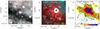 |
Fig. 1. Morphology of G11P1-HFS seen in the Spitzer, JWST, and ALMA observations. a) Spitzer 8 μm image. b) Two-color composite map made of the JWST ratio map (F444W/F356W; inverted scale in red) and Spitzer 8 μm (cyan) emission. Stars show the positions of compact radio continuum sources from Rosero et al. (2014). c) ALMA N2H+(1–0) integrated emission map overlaid with the footprints of structures seen in the JWST ratio map (see text for details). The color scale bar has a unit of Jy beam−1 km s−1. In each panel, a cross represents the position of the 6.7-GHz methanol maser. A dotted contour in panels “b” and “c” mark the Spitzer 8 μm emission feature. In panels “b” and “c”, arrows highlight possible filamentary features (F1–F6). Scale bar represents a physical scale of 0.3 pc at a distance of Galactic Snake (2.92 kpc; Dewangan et al. 2024). |
2. Datasets
This work primarily exploits the N2H+(1–0) line data from the ALMA Band-3 observations of IRDC_G011.11-4 (central coordinates: RA = 18h 10m 28.3s, Dec = −19d 22m 31s) obtained under the project code 2018.1.00424.S (PI: Gieser, Caroline). We retrieved the processed data from the ALMA archive. The angular resolution of the data cube was 4 712 × 2
 588 (0.07 × 0.037 pc2 at d = 2.92 kpc) with a pixel scale of 0
 46 (see observation details in Gieser et al. 2023). To complement the line data, we also utilized the Spitzer 8 μm image (resolution ∼2″; or ∼5840 au) and the JWST NIRCAM images at 3.563 and 4.421 μm (resolution ∼0
 17; or ∼500 au) from Paper I. Since N2H+ has a high critical density (4.4 × 105 cm−3 at 40 K), it can probe the high density regions (e.g., Pirogov et al. 2003). Though consisting of seven hyperfine observationally resolved components (e.g., Caselli et al. 1995; Daniel et al. 2006), N2H+(1–0) spectra show only three lines in our target region, two of which are triplets (see Fig. A.1a).
3. Analysis and results
Figure 1b shows the two-color composite image. The red color shows the JWST ratio map (F444W/F356W), and cyan is used to indicate the Spitzer 8 μm emission map of the G11P1 environment. The Spitzer/JWST ratio map (inverted scale) exhibits a strong morphological correlation with the mid-infrared emission and traces warm dusty features (see Fig. 4 in Bhadari et al. 2020 and Dewangan et al. 2023). At least six elongated structures (F1–F6; filaments, hereafter) are evident that connect to the central region hosting several compact radio continuum sources (CRCSs), including G11P1 and a 6.7 GHz methanol maser emission (see also Rosero et al. 2014). This traces a potential small-scale HFS (∼0.55 pc; Paper I) that needs confirmation through molecular line observations.
3.1. ALMA N2H+(1–0) emission
To compare the morphology of structures seen in the JWST images with the dense gas structures, we present the overlay of the JWST ratio map contours onto the N2H+(1–0) integrated emission map in Fig. 1c. The N2H+(1–0) emission is integrated over a velocity range from 25 to 32 km s−1, considering the major peak of N2H+(1–0) triplets (see Sect. 2). The N2H+(1–0) spectrum averaged over the HFS is shown in Fig. A.1a. To reduce noise and enhance the structures visible in the JWST images, we applied median filtering with a six-pixel width followed by smoothing of the resulting map with a 3 × 3 pixel2 box-car kernel. These parameters were chosen to achieve the optimal image presented in Fig. 1b (see also contours in Fig. 1c). We note that there is a significant similarity between the morphology of N2H+ emission and the structures traced by the JWST. This directly confirms the G11P1-HFS as an HFS seen at a small scale (< 0.6 pc). The N2H+(1–0) moment maps – for example, the integrated intensity, the intensity weighted centroid velocity (VLSR), and the intensity weighted line width, that is, full width at half maximum (FWHM; ΔVLSR) maps – are presented in Figs. A.2a–c, respectively. For comparison, we also present the moment-2 map derived using the N2H+(1–0) singlet F1 F = 01–12 (VLSR = [18, 23] km s−1) in Fig. A.2d.
To disentangle the multiple velocity components, we performed the spectral decomposition of the N2H+(1–0) emission using SCOUSEPY tool (Henshaw et al. 2016, 2019). The fitted centroid velocity in each pixel was used to generate a position-position-velocity (PPV) map, which is shown in Fig. 2. The five potential hub-forming filaments (F1–F5) are marked in the PPV map and in the moment-0 map shown at the bottom face of the PPV cube. A candidate filament, F6, observed in the JWST (Fig. 1b) may be blended with a potential outflow feature (see gas structure in VLSR > 31 and < 28 km s−1), so we excluded it from further analysis. Additionally, the F5 feature is not well resolved in the ALMA N2H+(1–0) map. Therefore, a tentative rectangular box is used for its analysis (see Sect. 3.2). The signature of velocity variations is evident along the filaments joining hub.
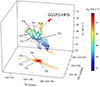 |
Fig. 2. Position–position–velocity map of ALMA N2H+(1–0) derived using the SCOUSEPY. The position-position space at the bottom of the map displays the integrated intensity map for the entire structure. Five filaments comprising G11P1-HFS are marked. The 3D view of the PPV map is available online. |
To quantify the on-sky velocity variation, we first derived the magnitude of velocity gradient (Vg) along the RA (𝒢α) and Dec (𝒢δ) directions as the second order central differences of VLSR. We estimated the resultant magnitude and position angle as  and
and  , respectively (see also Eswaraiah et al. 2020). Figure 3 displays the overlay of velocity gradient vectors2 with 2 × 2 pixel2 averaging on the peak-intensity map. The vectors converge to at least two peak intensity zones in the G11P1-hub, where dendrogram leaves (or cores) #L9 (∼22 M⊙) and #L14 (∼8 M⊙) are also identified (see following text). A noticeable feature is the gradual decrease of vector lengths as one moves toward these cores (or G11P1-hub centers). This feature is further quantified in Sect. 3.2 and Fig. 4. We utilized the Python-based astrodendro package to identify the hierarchical substructures in N2H+(1–0) PPV space. The input parameters, “min_value,” “min_delta,” and “min_npix” were set to be 5 sigma, 1 sigma, and 65 pixels, respectively, where 1 sigma (∼14 mJy beam−1) is the rms of the data. The dendrogram leaves (cores) are overlaid in Fig. 3, and their physical parameters are listed in Table A.1. The dendrogram tree of hierarchical structures (i.e., leaves and branches) is shown in Fig. A.1b.
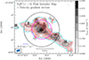 |
Fig. 3. Overlay of velocity gradient (Vg) vectors and dendrogram leaves on the N2H+(1–0) peak intensity map. The arrowheads point to local blueshifted velocity material. The reference Vg vector and ALMA beam are shown in the lower-left corner. The cyan contour presents the N2H+ emission at a level of 0.2 Jy beam−1 km s−1. Two circular regions, radii ∼12″ (∼0.17 pc) and 22″ (∼0.3 pc), typically mark the boundaries of the hub and G11P1-HFS (see text and Fig. 4). |
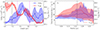 |
Fig. 4. Distribution of N(H2), VLSR, and Vg. (a) Distribution of N(H2) and VLSR along the rectangular strip shown in Fig. A.2a. The dots and shaded regions represent the mean and standard deviation range for each box in the strip. The dashed and solid vertical lines mark the boundary of two concentric circular regions shown in Fig. 3. (b) Radial plots for VLSR and Vg drawn from the center of concentric circles (Fig. 3). The vertical dotted-dashed line shows the boundary of the inner circle in Fig. 3. |
3.2. Gas-kinematics of G11P1-HFS
We derived the N2H+ column density, N(N2H+), and the excitation temperature (Tex) maps by modeling the fine structure components of N2H+(1–0) emission with XCLASS (Möller et al. 2017). The conversion factor 𝒳 = 3 × 10⁻¹⁰ was used to derive the H2 column density, N(H2), from N(N2H+) (Caselli et al. 2002). Figures A.2e and f present the N(H2) and Tex maps, respectively. Following the column density–mass relation (see Eq. (1) in Bhadari et al. 2020), the mass of the elongated feature enclosed by the N(H2) level of 3 × 1022 cm−2 was estimated to be ∼223 M⊙, which agrees with the mass of the dense source hosting G11P1 (see Sect. 1). The derived N(H2) and mass may have uncertainties of about 60–70% due to a potentially lower N2H+ abundance from chemical differentiation (Zinchenko et al. 2009) and high uncertainties itself in the calculation of 𝒳 for both low-mass and high-mass core samples (Caselli et al. 2002; Pirogov et al. 2013).
Figure 4a presents the N(H2) and VLSR distribution along a rectangular strip (from the northeast to southwest direction) marked in Fig. A.2a. A notable feature includes the simultaneous peak and dip in the N(H2) and VLSR profiles at G11P1-HFS center (or #L9), respectively. The steep velocity gradient is estimated to be −7 km s−1 pc−1 and 4.7 km s−1 pc−1 toward northeast and southwest side of the G11P1-HFS center, respectively. This strongly favors the presence of a mass accreting object (e.g., Zhou et al. 2023). We present an azimuthally averaged distribution of VLSR and Vg toward the G11P1-hub region in Fig. 4b. While the steep slope of VLSR indicates material flow toward the hub, the change in Vg might indicate the nature of the converging flows forming a hub (see Sect. 4.2). The N(H2) and VLSR profiles for the hub-joining filaments (F1–F5) are shown in Fig. A.3, and they indicate a significant velocity gradient toward the hub region. Almost all the VLSR profiles (except F1) show a sharp velocity gradient (∼8–15 km s−1 pc−1) up to ∼0.05 pc from the hub (see the last panel in Fig. A.3). This may be indicative of the hub radius; however, it is important to note that the profiles are not drawn from a common center due to the presence of at least two hub centers.
In order to estimate whether the gas flow along the hub composing filaments is driven by local gravity, we estimated the sky-projected gravitational force vectors (ℱg) using N(H2) map following the approach discussed in Wang et al. (2022, see Eq. (3) therein). The low relative angle between on-sky Vg and ℱg vectors along filaments (see Fig. B.1a; and details in Appendix B) hints the supportive role of gravity on mass assembly toward G11P1-HFS (e.g., Wang et al. 2022; Maity et al. 2024).
4. Discussion
4.1. Gas inflow along filaments
Material inflow along filaments is often inferred by the gradual change in gas velocity. Though the knowledge of the actual velocity gradient along filaments is elusive due to the unknown inclination of filaments, the on-sky VLSR variation along filaments is a key proxy that has been used in several studies (e.g., Kirk et al. 2013; Chen et al. 2019). The longitudinal gas flow along filaments may be driven by the self-gravity of embedded clumps (or cores), pressure-driven flows (or turbulence), the role of the magnetic field, or a combination of these factors. At smaller physical scales, the self-gravity of central hubs plays an important role (e.g., Zhou et al. 2022; Maity et al. 2024, and references therein). The signature of the velocity gradient along filaments in G11P1-HFS hints at the mass assembly process. The mass accretion rate along filaments (see boxed regions in Fig. A.2c) was found in the range of 0.92–1.44 M⊙ Myr−1 following the equation  , where ΔVobs, M, and α are the observed velocity gradient along the filament (0.075–0.12 km s−1 pc−1), filament mass (7.47–18.56 M⊙), and inclination angle of the filament in the sky plane (assumed to be 45°), respectively (see details in Kirk et al. 2013). Padoan et al. (2020) find that the mass-flow rate around prestellar cores increases linearly with size, with an average value of ∼10 M⊙ Myr−1 at 0.1 pc and ∼100 M⊙ Myr−1 at 1 pc. Similar results have also been reported in observational studies (e.g., Peretto et al. 2014; Yuan et al. 2018). Our derived values are two orders of magnitude less than the reported values. This discrepancy may be due to missing flux, which affects the mass and size of the filaments. Nevertheless, these results align with the GHC and I2 scenarios, supporting the idea that low-mass prestellar cores grow into high-mass protostars through continuous mass accretion from parent clumps or filamentary structures. Gravity appears to play a dominant role in mass accretion along filaments (see Fig. B.1), which is consistent with both the GHC and I2 models at core scales. However, to unveil the acting scale of gravity and turbulence, a systematic study consisting of interferometric and single-dish line observations can help (e.g., Hacar et al. 2018), but it is beyond the scope of the current work.
4.2. G11P1-HFS: An HFS at the nascent phase
Typically, once a high-mass star forms, it tends to disrupt the parent clump or cloud structure through its energetic feedback processes (e.g., strong ionization through extreme UV photons, stellar winds, and outflows; Motte et al. 2018; Schneider et al. 2020) and thereby diminishes the signature of their formation processes. In this context, tracing the undestroyed HFS hosting a young high-mass protostar becomes important to understanding the mass assembly in MSF processes. G11P1-HFS is one such site where the high-mass protostar G11P1 along with cluster members are embedded in a small-scale HFS. Probing the inner region of the parsec-scale hubs has only been possible with high-resolution ALMA observations (Kumar et al. 2020). Zhou et al. (2022) identified small-scale HFSs (≥0.1 pc) in a large sample of protoclusters using H13CO+(1–0) under the ATOMS survey. These observations are in line with our findings and the discussion of Kumar et al. (2022), which supports that HFSs are self-similar hierarchical structures observed at a physical scale ranging from protostellar envelope to the clump and cloud scales (i.e., ≥0.1 pc; Zhou et al. 2023; Bhadari et al. 2022, and references therein). The “V”-shaped VLSR profile in the direction of the hub, where the N(H2) profile peaks (see Fig. 4a), is a key signature of a spherically symmetric infall motion or mass-accreting hub (Zhou et al. 2023). Furthermore, the gradual decline of Vg toward dense cores (Figs. 3 and 4b) may indicate the coalescing nature of filaments toward the hub. This can be caused by the shock dissipation and the exchange of momentum between filaments with different velocities resulting in low Vg at flow-converging zones (Fukui et al. 2021). The regularly spaced cores #L10, #L8, #L9, #L13, and #L12 along the major filament spine (mean projected separation ∼0.22±0.02 pc; Fig. A.2a) suggest their formation through filament fragmentation processes (Inutsuka & Miyama 1992). This has also been observed in the vicinity of the high-mass protostar W42-MME (Bhadari et al. 2023), hinting that pristine hubs, and thus high-mass stars, form at the centers of their parent gas streams. The higher αvir values (Table A.1) suggest these dendrogram structures are transient, reflecting a dynamic and rapid mass assembly in the HFS.
The absence of extended radio emission, the presence of CRCSs, and mass-accreting structures suggest that G11P1-HFS is in its nascent phase3. In comparison, the nearby Mon R2 HFS (d = 830 pc), which has a similar physical scale (< 0.8 pc; Treviño-Morales et al. 2019; Kumar et al. 2022; Dewangan et al. 2025), appears to be relatively evolved, as it hosts an ultra-compact HII region and an embedded stellar cluster with at least two B-type stars at its hub center.
4.3. Wiggled funnel: Signature of HFSs in PPV space
Regardless of their extents, HFSs are recognized as converging filaments toward the position-position or 2D maps. However, their significance in mass assembly is underscored when these systems exhibit a “V” shape in position-velocity space or a funnel morphology in PPV space(see Fig. 9 in Zhou et al. 2023). The funnel signature may be feeble at cloud scales due to external feedback factors such as turbulence, outflows, and HII region feedback. At core scales, this signature can be discernible during early star-formation stages. G11P1-HFS presents an ideal site for such observations. Diverging from the ideal funnel structure, our observations reveal an azimuthally wiggling funnel structure of G11P1-HFS in PPV space. This idea is also supported by the study of G333, where HFSs display wiggling features in the PPV map, as shown by Zhou et al. (2023, see Fig. 6). These observations suggest the role of sub-filaments that feed the major filament connected to the hub, which are generally observed as transverse structures away from the hub. Figure A.4 presents the schematic diagram of the molecular clouds and the hierarchical filamentary substructures as they appear in PPV space.
5. Conclusions
The ALMA N2H+(1–0) observations confirm the presence of infrared-dark G11P1-HFS (< 0.6 pc) that was previously identified using JWST images. In addition to the V-shaped velocity profile toward the G11P1-hub (i.e., Vg of −7 and 5 km s−1 pc−1), the wiggled funnel feature observed in PPV space indicates the presence of a mass-accreting hub and the role of transverse gas flow. The low relative angle between the on-sky Vg and ℱg vectors hints at the gravity-driven inflow process along filaments.
Data availability
Interactive figure associated to Fig. 2 is available at https://www.aanda.org
We refer to large-scale HFSs with hub sizes of ∼1 pc or more, primarily observed in the Herschel maps (e.g., Kumar et al. 2020). In contrast, small-scale HFSs, observed with ALMA, exhibit clumps or hubs that split into elongated structures at sub-parsec scales, resembling HFSs, as noted by Zhou et al. (2022) in the ATOMS survey and Hacar et al. (2018) in the Orion Integral Filament.
The velocity gradient vectors were intentionally drawn pointing toward a decreasing velocity to make an easy comparison with the PPV map shown in Fig. 2.
We refer to the nascent phase of the HFS, which is at its lower hierarchy and still preserves the signature of multiple accreting filaments.
Acknowledgments
We thank the anonymous reviewer for useful comments and suggestions, which improved the quality of manuscript. The research work at the Physical Research Laboratory is funded by the Department of Space, Government of India. A portion of this research was carried out at the Jet Propulsion Laboratory, California Institute of Technology, under a contract with the National Aeronautics and Space Administration (80NM0018D0004). L.E.P. acknowledges the support of the Russian Science Foundation (project 24-12-00153). A.H.I. acknowledges the support from Ajman University, IRG No: [DGSR Ref. 2024-IRG-HBS-7]. This paper makes use of the following ALMA data: ADS/JAO.ALMA#2018.1.00424.S (https://jvo.nao.ac.jp/portal/alma/archive.do). ALMA is a partnership of ESO (representing its member states), NSF (USA) and NINS (Japan), together with NRC (Canada), MOST and ASIAA (Taiwan), and KASI (Republic of Korea), in cooperation with the Republic of Chile. The Joint ALMA Observatory is operated by ESO, AUI/NRAO and NAOJ. This work is based (in part) on observations made with the NASA/ESA/CSA JWST. The data were obtained from the Mikulski Archive for Space Telescopes at the Space Telescope Science Institute, which is operated by the Association of Universities for Research in Astronomy, Inc., under NASA contract NAS 5-03127 for JWST. These observations are associated with the programme #1182. This research made use of astrodendro, a Python package to compute dendrograms of Astronomical data (http://www.dendrograms.org/). This work made use of Astropy: (http://www.astropy.org) a community-developed core Python package and an ecosystem of tools and resources for astronomy (Astropy Collaboration 2013); astropy:2022.
References
- Astropy Collaboration (Robitaille, T. P., et al.) 2013, A&A, 558, A33 [NASA ADS] [CrossRef] [EDP Sciences] [Google Scholar]
- Astropy Collaboration (Price-Whelan, A. M., et al.) 2022, ApJ, 935, 167 [NASA ADS] [CrossRef] [Google Scholar]
- Bhadari, N. K., Dewangan, L. K., Pirogov, L. E., & Ojha, D. K. 2020, ApJ, 899, 167 [NASA ADS] [CrossRef] [Google Scholar]
- Bhadari, N. K., Dewangan, L. K., Ojha, D. K., Pirogov, L. E., & Maity, A. K. 2022, ApJ, 930, 169 [NASA ADS] [CrossRef] [Google Scholar]
- Bhadari, N. K., Dewangan, L. K., Pirogov, L. E., et al. 2023, MNRAS, 526, 4402 [NASA ADS] [CrossRef] [Google Scholar]
- Bonnell, I. A., & Bate, M. R. 2006, MNRAS, 370, 488 [NASA ADS] [CrossRef] [Google Scholar]
- Carey, S. J., Clark, F. O., Egan, M. P., et al. 1998, ApJ, 508, 721 [Google Scholar]
- Caselli, P., Myers, P. C., & Thaddeus, P. 1995, ApJ, 455, L77 [Google Scholar]
- Caselli, P., Benson, P. J., Myers, P. C., & Tafalla, M. 2002, ApJ, 572, 238 [Google Scholar]
- Chen, H.-R. V., Zhang, Q., Wright, M. C. H., et al. 2019, ApJ, 875, 24 [Google Scholar]
- Daniel, F., Cernicharo, J., & Dubernet, M. L. 2006, ApJ, 648, 461 [NASA ADS] [CrossRef] [Google Scholar]
- Dewangan, L. K., Ojha, D. K., Sharma, S., et al. 2020, ApJ, 903, 13 [Google Scholar]
- Dewangan, L. K., Zinchenko, I. I., Zemlyanukha, P. M., et al. 2022, ApJ, 925, 41 [NASA ADS] [CrossRef] [Google Scholar]
- Dewangan, L. K., Maity, A. K., Mayya, Y. D., et al. 2023, ApJ, 958, 51 [NASA ADS] [CrossRef] [Google Scholar]
- Dewangan, L. K., Bhadari, N. K., Maity, A. K., et al. 2024, MNRAS, 527, 5895 [Google Scholar]
- Dewangan, L. K., Bhadari, N. K., Maity, A. K., et al. 2025, AJ, 169, 80 [NASA ADS] [CrossRef] [Google Scholar]
- Eswaraiah, C., Li, D., Samal, M. R., et al. 2020, ApJ, 897, 90 [Google Scholar]
- Fukui, Y., Inoue, T., Hayakawa, T., & Torii, K. 2021, PASJ, 73, S405 [Google Scholar]
- Gieser, C., Beuther, H., Semenov, D., et al. 2023, A&A, 674, A160 [NASA ADS] [CrossRef] [EDP Sciences] [Google Scholar]
- Gómez, G. C., & Vázquez-Semadeni, E. 2014, ApJ, 791, 124 [Google Scholar]
- Hacar, A., Clark, S. E., Heitsch, F., et al. 2023, in Protostars and Planets VII, eds. S. Inutsuka, Y. Aikawa, T. Muto, K. Tomida, & M. Tamura, ASP Conf. Ser., 534, 153 [NASA ADS] [Google Scholar]
- Hacar, A., Tafalla, M., Forbrich, J., et al. 2018, A&A, 610, A77 [NASA ADS] [CrossRef] [EDP Sciences] [Google Scholar]
- Henshaw, J. D., Longmore, S. N., Kruijssen, J. M. D., et al. 2016, MNRAS, 457, 2675 [Google Scholar]
- Henshaw, J. D., Ginsburg, A., Haworth, T. J., et al. 2019, MNRAS, 485, 2457 [Google Scholar]
- Inutsuka, S.-I., & Miyama, S. M. 1992, ApJ, 388, 392 [CrossRef] [Google Scholar]
- Kauffmann, J., & Pillai, T. 2010, ApJ, 723, L7 [Google Scholar]
- Kirk, H., Myers, P. C., Bourke, T. L., et al. 2013, ApJ, 766, 115 [Google Scholar]
- Kumar, M. S. N., Palmeirim, P., Arzoumanian, D., & Inutsuka, S. I. 2020, A&A, 642, A87 [EDP Sciences] [Google Scholar]
- Kumar, M. S. N., Arzoumanian, D., Men’shchikov, A., et al. 2022, A&A, 658, A114 [NASA ADS] [CrossRef] [EDP Sciences] [Google Scholar]
- Maity, A. K., Inoue, T., Fukui, Y., et al. 2024, ApJ, 974, 229 [NASA ADS] [CrossRef] [Google Scholar]
- McKee, C. F., & Tan, J. C. 2003, ApJ, 585, 850 [Google Scholar]
- Möller, T., Endres, C., & Schilke, P. 2017, A&A, 598, A7 [NASA ADS] [CrossRef] [EDP Sciences] [Google Scholar]
- Motte, F., Bontemps, S., & Louvet, F. 2018, ARA&A, 56, 41 [NASA ADS] [CrossRef] [Google Scholar]
- Myers, P. C. 2009, Astrophysical Journal, 700, 1609 [NASA ADS] [CrossRef] [Google Scholar]
- Padoan, P., Pan, L., Juvela, M., Haugbølle, T., & Nordlund, Å. 2020, ApJ, 900, 82 [NASA ADS] [CrossRef] [Google Scholar]
- Peretto, N., Fuller, G. A., André, P., et al. 2014, A&A, 561, A83 [NASA ADS] [CrossRef] [EDP Sciences] [Google Scholar]
- Peretto, N., Fuller, G. A., Duarte-Cabral, A., et al. 2013, A&A, 555, A112 [NASA ADS] [CrossRef] [EDP Sciences] [Google Scholar]
- Pirogov, L., Zinchenko, I., Caselli, P., Johansson, L. E. B., & Myers, P. C. 2003, A&A, 405, 639 [NASA ADS] [CrossRef] [EDP Sciences] [Google Scholar]
- Pirogov, L., Ojha, D. K., Thomasson, M., Wu, Y. F., & Zinchenko, I. 2013, MNRAS, 436, 3186 [NASA ADS] [CrossRef] [Google Scholar]
- Rosero, V., Hofner, P., McCoy, M., et al. 2014, ApJ, 796, 130 [NASA ADS] [CrossRef] [Google Scholar]
- Schneider, N., Simon, R., Guevara, C., et al. 2020, PASP, 132, 1 [Google Scholar]
- Treviño-Morales, S. P., Fuente, A., Sánchez-Monge, Á., et al. 2019, A&A, 629, A81 [NASA ADS] [CrossRef] [EDP Sciences] [Google Scholar]
- Vázquez-Semadeni, E., Palau, A., Ballesteros-Paredes, J., Gómez, G. C., & Zamora-Avilés, M. 2019, MNRAS, 490, 3061 [Google Scholar]
- Vázquez-Semadeni, E., Gómez, G. C., & González-Samaniego, A. 2024, MNRAS, 530, 3445 [CrossRef] [Google Scholar]
- Wang, K., Zhang, Q., Testi, L., et al. 2014, MNRAS, 439, 3275 [Google Scholar]
- Wang, J.-W., Koch, P. M., Tang, Y.-W., et al. 2022, ApJ, 931, 115 [NASA ADS] [CrossRef] [Google Scholar]
- Yang, D., Liu, H.-L., Tej, A., et al. 2023, ApJ, 953, 40 [NASA ADS] [CrossRef] [Google Scholar]
- Yuan, J., Li, J.-Z., Wu, Y., et al. 2018, ApJ, 852, 12 [Google Scholar]
- Zhou, J.-W., Liu, T., Evans, N. J., et al. 2022, MNRAS, 514, 6038 [NASA ADS] [CrossRef] [Google Scholar]
- Zhou, J. W., Wyrowski, F., Neupane, S., et al. 2023, A&A, 676, A69 [NASA ADS] [CrossRef] [EDP Sciences] [Google Scholar]
- Zinchenko, I., Caselli, P., & Pirogov, L. 2009, MNRAS, 395, 2234 [NASA ADS] [CrossRef] [Google Scholar]
Appendix A: Figures
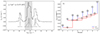 |
Fig. A.1. a) N2H+(1–0) spectrum averaged over the G11P1-HFS region (see the larger circle in Fig. 3). The seven hyperfine components are labeled. The shaded region shows the central peak with VLSR ranging from 25 to 32 km s−1, which is used for the gas kinematics study (Sec. 3.2). b) Dendrogram tree of N2H+(1–0) emission. The leaves and branches are marked (see also Fig. 3). |
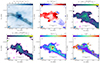 |
Fig. A.2. (a–c) Moment-0/1/2 maps of N2H+(1–0) emission derived using central peak (see shaded area in A.1a). d) Moment-2 map of N2H+(1–0) emission made using singlet F1 F = 01–12. e) H2 column density and f) excitation temperature maps. In panel (e), overlaid contour is of N2H+(1–0) integrated emission at the level of 0.2 Jy beam−1 km s−1. The star and cross symbols are same as shown in Fig. 1. The apertures of identified cores, and a rectangular strip are overlaid in panel (a). In panel (c), rectangular boxes mark areas of hub-composing filaments (F1-F5). A contour in panels (c) and (d) displays structure traced by the JWST (see Fig. 1c). |
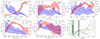 |
Fig. A.3. Distribution of N(H2) and VLSR along the five filaments (F1–F5), from the head (or hub) to the tail (see boxes in Fig. A.2c). The shaded regions are the same as in Fig. 4. The bottom-right panel shows the VLSR profiles of all filaments. Shadowed regions mark the hub center, and the position ranges from 0.04 to 0.055 pc. |
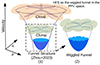 |
Fig. A.4. Schematic diagram of the hierarchical HFSs in PPV space as a funnel structure (1) discussed by Zhou et al. (2023) and a (2) wiggled funnel that reveals the role of sub-filaments. |
Physical parameters of dendrogram leaves for G11P1-HFS.
Appendix B: Distribution of on-sky gravity, velocity, and intensity vectors
The relative orientation between possible pairs of ℱg, Vg, and intensity gradient (Ig; derived using moment-0 map) was estimated neglecting the true vector direction, thereby converging angle difference (Δθi, j) is in the range of 0–90°, where i and j refer to two different parameters (i.e., velocity gradient (v), intensity gradient (i), and gravity (g)). Fig. B.1a displays the spatial distribution of Δθv, g toward G11P1-HFS. To highlight the filament positions, we have overlaid the JWST ratio map contour (see Fig. 1c). Interestingly, along the filament spines, the Δθv, g values are significantly low, indicating that the Vg and ℱg vectors are well aligned in these areas compared to other locations. Fig. B.1b shows the histogram distribution of Δθv, g, Δθi, g, and Δθi, v toward the entire G11P1-HFS. The Δθv, g shown in Fig. B.1b have mean/median values of approximately 41°/39°, highlighting the dominant role of gravity in mass accretion process.
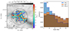 |
Fig. B.1. Distribution of relative orientation between gravity (g), velocity gradient (v), and intensity gradient (i) vectors. a) Spatial distribution of relative orientation between g and v vectors (in color) overlaid on the N2H+ moment-0 map. b) Histogram distribution of relative orientation between g, v, and i vectors toward circular region marked in panel (a). Black and cyan contours are same as the contours shown in Fig. A.2c, and Fig. A.2e, respectively. |
All Tables
All Figures
|
Fig. 1. Morphology of G11P1-HFS seen in the Spitzer, JWST, and ALMA observations. a) Spitzer 8 μm image. b) Two-color composite map made of the JWST ratio map (F444W/F356W; inverted scale in red) and Spitzer 8 μm (cyan) emission. Stars show the positions of compact radio continuum sources from Rosero et al. (2014). c) ALMA N2H+(1–0) integrated emission map overlaid with the footprints of structures seen in the JWST ratio map (see text for details). The color scale bar has a unit of Jy beam−1 km s−1. In each panel, a cross represents the position of the 6.7-GHz methanol maser. A dotted contour in panels “b” and “c” mark the Spitzer 8 μm emission feature. In panels “b” and “c”, arrows highlight possible filamentary features (F1–F6). Scale bar represents a physical scale of 0.3 pc at a distance of Galactic Snake (2.92 kpc; Dewangan et al. 2024). |
| In the text | |
|
Fig. 2. Position–position–velocity map of ALMA N2H+(1–0) derived using the SCOUSEPY. The position-position space at the bottom of the map displays the integrated intensity map for the entire structure. Five filaments comprising G11P1-HFS are marked. The 3D view of the PPV map is available online. |
| In the text | |
|
Fig. 3. Overlay of velocity gradient (Vg) vectors and dendrogram leaves on the N2H+(1–0) peak intensity map. The arrowheads point to local blueshifted velocity material. The reference Vg vector and ALMA beam are shown in the lower-left corner. The cyan contour presents the N2H+ emission at a level of 0.2 Jy beam−1 km s−1. Two circular regions, radii ∼12″ (∼0.17 pc) and 22″ (∼0.3 pc), typically mark the boundaries of the hub and G11P1-HFS (see text and Fig. 4). |
| In the text | |
|
Fig. 4. Distribution of N(H2), VLSR, and Vg. (a) Distribution of N(H2) and VLSR along the rectangular strip shown in Fig. A.2a. The dots and shaded regions represent the mean and standard deviation range for each box in the strip. The dashed and solid vertical lines mark the boundary of two concentric circular regions shown in Fig. 3. (b) Radial plots for VLSR and Vg drawn from the center of concentric circles (Fig. 3). The vertical dotted-dashed line shows the boundary of the inner circle in Fig. 3. |
| In the text | |
|
Fig. A.1. a) N2H+(1–0) spectrum averaged over the G11P1-HFS region (see the larger circle in Fig. 3). The seven hyperfine components are labeled. The shaded region shows the central peak with VLSR ranging from 25 to 32 km s−1, which is used for the gas kinematics study (Sec. 3.2). b) Dendrogram tree of N2H+(1–0) emission. The leaves and branches are marked (see also Fig. 3). |
| In the text | |
|
Fig. A.2. (a–c) Moment-0/1/2 maps of N2H+(1–0) emission derived using central peak (see shaded area in A.1a). d) Moment-2 map of N2H+(1–0) emission made using singlet F1 F = 01–12. e) H2 column density and f) excitation temperature maps. In panel (e), overlaid contour is of N2H+(1–0) integrated emission at the level of 0.2 Jy beam−1 km s−1. The star and cross symbols are same as shown in Fig. 1. The apertures of identified cores, and a rectangular strip are overlaid in panel (a). In panel (c), rectangular boxes mark areas of hub-composing filaments (F1-F5). A contour in panels (c) and (d) displays structure traced by the JWST (see Fig. 1c). |
| In the text | |
|
Fig. A.3. Distribution of N(H2) and VLSR along the five filaments (F1–F5), from the head (or hub) to the tail (see boxes in Fig. A.2c). The shaded regions are the same as in Fig. 4. The bottom-right panel shows the VLSR profiles of all filaments. Shadowed regions mark the hub center, and the position ranges from 0.04 to 0.055 pc. |
| In the text | |
|
Fig. A.4. Schematic diagram of the hierarchical HFSs in PPV space as a funnel structure (1) discussed by Zhou et al. (2023) and a (2) wiggled funnel that reveals the role of sub-filaments. |
| In the text | |
|
Fig. B.1. Distribution of relative orientation between gravity (g), velocity gradient (v), and intensity gradient (i) vectors. a) Spatial distribution of relative orientation between g and v vectors (in color) overlaid on the N2H+ moment-0 map. b) Histogram distribution of relative orientation between g, v, and i vectors toward circular region marked in panel (a). Black and cyan contours are same as the contours shown in Fig. A.2c, and Fig. A.2e, respectively. |
| In the text | |
Current usage metrics show cumulative count of Article Views (full-text article views including HTML views, PDF and ePub downloads, according to the available data) and Abstracts Views on Vision4Press platform.
Data correspond to usage on the plateform after 2015. The current usage metrics is available 48-96 hours after online publication and is updated daily on week days.
Initial download of the metrics may take a while.