| Issue |
A&A
Volume 694, February 2025
|
|
|---|---|---|
| Article Number | A100 | |
| Number of page(s) | 25 | |
| Section | Extragalactic astronomy | |
| DOI | https://doi.org/10.1051/0004-6361/202450426 | |
| Published online | 10 February 2025 | |
The MUSE eXtremely Deep Field
Classifying the spectral shapes of Lyα-emitting galaxies
1
Observatoire de Genève, Université de Genève, Chemin Pegasi 51, 1290 Versoix, Switzerland
2
ESO Vitacura, Alonso de Córdova 3107, Vitacura, Casilla, 19001 Santiago de Chile, Chile
3
Department of Astronomy, The University of Texas at Austin, 2515 Speedway, Stop C1400 Austin, TX 78712-1205, USA
4
Kapteyn Astronomical Institute, University of Groningen, PO Box 800 NL-9700 AV Groningen, The Netherlands
5
National Astronomical Observatory of Japan (NAOJ), 2-21-1 Osawa, Mitaka, Tokyo 181-8588, Japan
6
Department of Physics, ETH Zürich, Wolfgang-Pauli-Strasse 27, Zürich 8093, Switzerland
7
Institute of Science and Technology Austria (IST Austria), Am Campus 1, Klosterneuburg, Austria
8
Univ. Lyon, Univ. Lyon1, ENS de Lyon, CNRS, Centre de Recherche Astrophysique de Lyon UMR5574, 69230 Saint-Genis-Laval, France
9
Department of Astronomy, University of Wisconsin-Madison, 475 N. Charter St., Madison, WI 53706, USA
10
Leibniz-Institut fur Astrophysik Potsdam (AIP), An der Sternwarte 16, 14482 Potsdam, Germany
11
Leiden Observatory, Leiden University, PO Box 9513 2300 RA Leiden, The Netherlands
12
Max Planck Institute for Astronomy, Königstuhl 17, D-69117 Heidelberg, Germany
13
JWST Australian Data Centre, Centre for Astrophysics and Supercomputing, Swinburne University of Technology, Victoria 3122, Australia
14
Institut de Recherche en Astrophysique et Planétologie (IRAP), Université de Toulouse, CNRS, UPS, CNES, 31400 Toulouse, France
⋆ Corresponding author; This email address is being protected from spambots. You need JavaScript enabled to view it.
Received:
17
April
2024
Accepted:
21
November
2024
Abstract
Context. The hydrogen Lyman-alpha (Lyα) line, the brightest rest-frame ultraviolet line of high-redshift galaxies, exhibits a large variety of shapes, which is due to factors at different scales, from the interstellar medium to the intergalactic medium (IGM).
Aims. The aim of this work is to provide a systematic inventory and classification of the spectral shapes of Lyα emission lines to better understand the general population of high-redshift Lyα emitting galaxies (LAEs).
Methods. Using the unprecedentedly deep data from the MUSE eXtremely Deep Field (MXDF; up to 140 hour exposure time), we selected 477 galaxies observed in the ∼2.8−6.6 redshift range, 15 of which have a systemic redshift from nebular lines. We developed a method to classify Lyα emission lines in four spectral and three spatial categories by combining a pure spectral analysis with a narrow-band image analysis. We measured spectral properties, such as the peak separation and the blue-to-total flux ratio for the double-peaked galaxies.
Results. To ensure a robust sample for statistical analysis, we define two unbiased subsets, inclusive and restrictive, by applying thresholds for signal-to-noise ratio, peak separation, and Lyα luminosity, yielding a final unbiased sample of 206 galaxies. Our analysis reveals that between 32% and 51% of the galaxies exhibit double-peaked profiles, with peak separations ranging from 150 km s−1 to nearly 1600 km s−1. The fraction of double-peaked galaxies seems to evolve dependently with the Lyα luminosity, while we do not see a severe decrease in this fraction with redshift, which is expected given the IGM attenuation at high redshift. An artificial increase in the number of double-peaked galaxies at the highest redshifts may cause the observation of a plateau instead of a decrease. A notable number of these double-peaked profiles show blue-dominated spectra, suggesting unique gas dynamics and inflow characteristics in some high-redshift galaxies. The consequent fraction of blue-dominated spectra needs to be confirmed by obtaining new systemic redshift measurements. Among the double-peaked galaxies, 4% are spurious detections, that is, the blue and red peaks do not come from the same spatial location. Around 20% out of the 477 sources of the parent sample lie in a complex environment, meaning there are other clumps or galaxies at the same redshift within a distance of 30 kpc.
Conclusions. Our results suggest that the double-peaked LAE fraction may trace the evolution of IGM attenuation, but the faintest galaxies must be observed at high redshift. We also need more data to confirm the trend seen at low redshift. In addition, it is crucial to obtain secure systemic redshifts for LAEs to better constrain the nature of the Lyα double-peaked lines. Statistical samples of double-peaked and triple-peaked galaxies are a promising probe of the evolution of the physical properties of galaxies across cosmic time.
Key words: galaxies: evolution / galaxies: formation / galaxies: high-redshift / cosmology: observations
© The Authors 2025
 Open Access article, published by EDP Sciences, under the terms of the Creative Commons Attribution License (https://creativecommons.org/licenses/by/4.0), which permits unrestricted use, distribution, and reproduction in any medium, provided the original work is properly cited.
This article is published in open access under the Subscribe to Open model. This email address is being protected from spambots. You need JavaScript enabled to view it. to support open access publication.
1. Introduction
The Lyman-alpha (Lyα, λ1216 Å) line of hydrogen, as the brightest ultraviolet (UV) line of star-forming galaxies (Partridge & Peebles 1967), is a key spectral feature in the observation of high-redshift galaxies, and is often the only detected signal (e.g. Rhoads et al. 2004; Malhotra & Rhoads 2004; Maseda et al. 2018). A remarkable characteristic of this line is the wide diversity of spectral shapes reported in the literature, at every redshift (e.g. Kulas et al. 2012; Henry et al. 2015; Yang et al. 2016; Leclercq et al. 2017; Kerutt et al. 2022). The archetypical Lyα shape is easily identifiable, showing a single red asymmetric line profile (e.g. Shapley et al. 2003; Tapken et al. 2007), but over the last decade, double-peaked Lyα lines have been observed (Henry et al. 2015; Hu et al. 2016; Matthee et al. 2018; Songaila et al. 2018; Meyer et al. 2021; Hayes et al. 2021) as well as triple-peaked ones (e.g. Vanzella et al. 2016, 2018; Naidu et al. 2017; Izotov et al. 2018; Rivera-Thorsen et al. 2019). The observation of this wide diversity of line shapes has become possible thanks to the emergence of instruments such as the Cosmic Origins Spectrograph on board the Hubble Space Telescope (HST/COS, Green et al. 2012), which observed low-z Lyα-emitting galaxies, the Multi-Unit Spectroscopic Explorer at the Very Large Telescope (VLT/MUSE, Bacon et al. 2010), which has unveiled a large population of faint star-forming galaxies at z = 3 − 6 (Bacon et al. 2023), and the Near-Infrared Spectrograph on board the James Webb Space Telescope (JWST/NIRSpec), which is already pushing the limits of Lyα-line observation towards higher redshifts (Bunker et al. 2023). The wavelength coverage of these instruments, ranging from UV to infrared (IR), enables the scientific community to observe the evolution of galaxies over a time span of approximately 13 Gyr using the same indicator: the Lyα line.
The observed diversity of spectral shapes arises from the resonant nature of the Lyα line (see e.g. Dijkstra 2017, for a review on Lyα radiation transfer effects in galaxies). Therefore, depending on the sightline, the shape of the Lyα line profile may vary drastically (Blaizot et al. 2023). The observed Lyα line profiles encode information on the gas velocity and its density distribution as the Lyα photons travel through the interstellar medium (ISM). For double-peaked Lyα lines (hereafter referred to as double-peaks), in particular, Verhamme et al. (2015) suggest that the separation between the two peaks of the Lyα line correlates with the neutral hydrogen column density. Indeed, a relationship between the Lyα peak separation and the Lyman-continuum (LyC) escape fraction has been found empirically for low-z LyC leakers (Verhamme et al. 2017; Izotov et al. 2021; Flury et al. 2022) and has been used at higher redshift on samples of Lyα-emitting galaxies (LAEs) to select LyC-leaking candidates (Naidu et al. 2022; Kramarenko et al. 2024). Nevertheless, Kerutt et al. (2024) could not confirm this relationship with their LAE sample at z = 3 − 4. The value of the blue-to-total flux ratio (B/T), another spectral property containing physical information, characterises the gas exchanges between the galaxy and its surrounding environment. In simulations, expanding shells produce red-dominated Lyα lines (i.e. B/T < 0.5, Verhamme et al. 2006), whereas blue-dominated spectra are seen when gas falls into the galaxy (Blaizot et al. 2023). The brightest Lyα phases of galaxies seem to be outflow phases (Blaizot et al. 2023). In observations, more red-dominated spectra have been observed than blue-dominated ones (Kulas et al. 2012; Trainor et al. 2015). A detailed analysis has only been done for a few blue-dominated objects (Mukherjee et al. 2023; Furtak et al. 2022; Marques-Chaves et al. 2022). Finally, the intergalactic medium (IGM) transmission decreases with increasing redshift, preferentially suppressing flux on the blue part of the Lyα line (Laursen et al. 2011; Garel et al. 2021; Hayes et al. 2021). To quantify the inflow and outflow phases, constrain the duty cycle of galaxies, and to study LyC leakers across different redshifts, it is important to measure the peak separation and the B/T flux ratio for a large number of galaxies over a large redshift range.
Until now, the diversity of the Lyα line profile has been quantified by dedicated surveys targeting previously detected LAEs. Kulas et al. (2012) found 30% of their UV-selected galaxy sample at z = 2 − 3 to be double-peaks and Yamada et al. (2012) found a fraction of double-peaks of 50% for z = 3.1 equivalent width (EW)-selected LAEs. Kerutt et al. (2022) found 33% of double-peaks for LAEs with z < 4 in the MUSE-Wide blind survey (Urrutia et al. 2019). The way the double-peaks are identified among a population of LAEs introduces biases. Indeed, most of the time the double-peaks are visually identified (e.g. Sobral et al. 2018) or a combination of a detection algorithm and visual inspection is used (Kulas et al. 2012). In this study, we use for the first time an automatic algorithm on a blind survey without pre-selection to quantify the diversity of the Lyα lines, both spectrally and spatially.
This paper is structured as follows. In Sect. 2, we describe the MUSE-Deep data and the sample selection. Section 3 is dedicated to the description of the method developed for identifying and characterising the spectral profiles of the Lyα lines of our sample of galaxies. In Sect. 4, we present the results of the classification and the fraction of double-peaks. The results are discussed in Sect. 5. Finally, we present a summary of our findings and our conclusions in Sect. 6. Throughout this paper, we assume a ΛCDM cosmology with Ωm = 0.3, ΩΛ = 0.7, and H0 = 67.4 km s−1 Mpc−1.
2. Data and sample definition
We constructed a sample of z-selected galaxies from the Data Release 2 (DR2) catalogue (Bacon et al. 2023, hereafter B23) of the MUSE eXtremely Deep Field (hereafter MXDF) to identify and characterise their Lyα emission line λ1216 Å based on publicly available spectra1. Our data set is described in Sect. 2.1. Sect. 2.2 is dedicated to our sample selection and finally, the choice of spectral extraction is discussed in Sect. 2.3.
2.1. Data set
The MXDF data were taken as part of the MUSE guaranteed time observations (GTO) program between August 2018 and January 2019. All observations were performed using the MUSE ground-layer adaptive optics (GLAO) mode. Details about the MXDF data processing and the production of the source catalogues can be found in the survey paper B23. In summary, a single pointing with the deepest exposure time of 140 hours was achieved. The final MXDF field of view has a circular shape designed to minimise systematics, with the following centre coordinates: 53 16467, −27
 78537 (J2000 FK5). The exposure time of the field exceeds 100 hours in the inner 31″ radius, which represents an area of 0.84 arcmin2, while it reaches around ten hours at a radius of 41″ (area of 1.47 arcmin2, Fig. 1). The 50% Lyα detection completeness, in the deepest 140-hour area, is achieved for an AB magnitude of 28.7 (F775W) at z = 3.2 − 4.5. The field overlaps partially with the other MUSE Hubble Ultra Deep Fields (HUDF, Bacon et al. 2017) of 31-hour (1 × 1 arcmin2) and 10-hour (3 × 3 arcmin2) total exposure times, called UDF-10 and MOSAIC, respectively. The 50% completeness is reached at 26.5 mag and 25.5 mag (z ∼ 4) in HST F775W, in UDF-10 and MOSAIC, respectively. The MXDF is two orders of magnitude deeper than UDF-10.
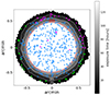 |
Fig. 1. Exposure time map of the MXDF. The blue circles are the MXDF-selected objects, the pink triangles indicate the UDF-10-selected targets and the green squares the MOSAIC-selected objects (see Sect. 2.2). The field is coloured by exposure time in hours, from 0 h to 140 h. The red contour represents the 100 h limit of the field. The solid and dashed white contours show the 30 h and 10 h exposure time of the MXDF, respectively. The UDF-10-selected objects present in the deepest part of the field have their Lyα line in the AO gap. |
The MXDF data cover a wavelength range from 4700 Å to 9350 Å excluding an adaptive optics (AO) gap from 5800 Å to 5966.25 Å due to the notch filter that blocks the bright light from the four sodium laser guide stars. Both the UDF-10 and MOSAIC fields were observed without AO and therefore do not have any AO gap in wavelength. In the MXDF, the full-width at half maximum (FWHM) of the Moffat point spread function (Moffat PSF, Moffat 1969) is 0.6″ at 4700 Å and 0.4″ at 9350 Å. The line spread function (LSF) of the MXDF is constant in the field and larger in the outer parts. The mean MXDF LSF over the wavelength range is 2.6 Å, which corresponds to a LSF of ≈150 km s−1 at z = 3 and ≈90 km s−1 at z = 6 (see details in Sect. 4.2.2 of B23).
The data reduction process performed on the DR2 survey is similar to the one for the Data Release 1 survey and is described in Bacon et al. (2017). However, some improvements have been made, especially in the sky-subtraction process (Appendix B of B23). The output data of the MXDF is a 3D datacube with dimensions of 3721 × 470 × 470 pixels, meaning that for each spatial pixel of  , a spectrum divided into 3721 pixels of 1.25 Å width is available. On top of the signal datacube, a variance datacube is provided.
2.2. Catalogue and data-set selection
The DR2 catalogue compiles all sources observed in the three MUSE Ultra Deep fields: MOSAIC (9 arcmin2), UDF-10 (1 arcmin2) and MXDF (1.47 arcmin2) (see Fig. 2 of B23). This catalogue contains 2221 sources, from nearby galaxies (z < 0.25) to high-redshift galaxies (up to z ≈ 6.64). The Lyα line is observable by MUSE in the redshift range z = 2.87 − 6.64. While a total of 1308 DR2 sources have their redshift in this range, not all have a strong Lyα line. Indeed, the Lyα emission can be faint, not detected, or in absorption.
For this study, we decided to restrict our analysis to the deepest data available, that is the MXDF field, to develop our method. The analysis of MOSAIC and UDF-10 will be the subject of future work. The first step in building our parent sample consists of selecting the objects detected in the 1.47 arcmin2MXDF field of view, with a spectroscopic redshift above 2.87. This reduces the number of galaxies from 1308 to 504. We did use the MOSAIC or UDF-10 data sets of a given source if (i) the data depth is deeper than in the MXDF data set at the location of the source (i.e. higher signal-to-noise ratio, hereafter S/N), which corresponds to 53 sources, or (ii) the Lyα line falls in the MXDF AO gap (five sources, see Fig. 1). After a cautious examination, 26 objects were removed from the parent sample because of misclassification in the DR2 catalogue. In addition, a last source has also been removed because the segmentation map used to extract the spectrum is on another galaxy. The distribution of our 477 galaxies is as follows (see Table 1):
-
419 galaxies have their deepest observations in the MXDF data set (blue circles in Fig. 1).
-
34 sources have their deepest observations in the UDF-10 data set (with a maximum of 30 hours of observations, pink triangles in Fig. 1).
-
24 have their deepest observations in the MOSAIC field (green squares in Fig. 1), accumulating a total of ten hours of integration.
In the DR2 catalogue, the redshift confidence parameter, ZCONF, indicates the reliability of the redshift solution (see B23). This parameter can range from zero to three, zero being the least confident redshift solution, and three the most secure one (see Sect. 5.3.7 of B23). Generally, when a source with a Lyα line is assigned a ZCONF = 2 or 3, it means that the S/N of the Lyα line is above five or seven, respectively. If a source can be matched to an HST counterpart, it adds confidence to the detection. In addition, if the photometric redshift of Rafelski et al. (2015) is reliable and matches with the MUSE redshift, this also increases the confidence of the redshift measurement. The presence of other nebular lines (such as C IV, He II, [O II] and [O III]) with reliable S/N in the spectrum also increases the confidence level of the redshift. If a source is assigned a redshift confidence level of one, there can be various reasons. It could be either due to a low S/N of the lines, noisy observations, other potential redshift solutions, or the presence of additional lines with good enough S/N in the spectrum but unexplained by the proposed redshift solution. In the specific case of low S/N spectra with a single emission line, to avoid misclassifications, B23 estimated the expected fraction of Lyα and [O II] emitters as other emission lines are much less likely because of the small accessible volume. The likelihood of misclassified lines is less than 10%, even for the faintest galaxies (i.e. fainter than F775W = 28.5, B23). Out of the 477 sources:
-
170 have a secure redshift, ZCONF = 3
-
161 sources have a confident redshift, ZCONF = 2
-
146 sources do not have a reliable spectroscopic redshift solution, ZCONF = 1.
To be inclusive, we did not make any selection based on the redshift confidence level. Only three of the sources with ZCONF = 1 passed the selection to be part of the unbiased sample (Sect. 4.1.3). Two of them are single-peak and one is a double-peak. Hence their inclusion in the unbiased parent sample does not impact our findings on the fraction of double-peaked LAEs, as detailed in Sect. 4.3.1. We still verified the impact of the ZCONF = 1 objects on the different distributions shown in Fig. 8 and confirmed that their inclusion or rejection does not modify these distributions.
2.3. Spectral extraction
Since MUSE is an integral-field unit spectrograph, the produced data format is a 3D datacube, from which spectra can be extracted in different ways. Bacon et al. (2023) used three different methods to extract the spectra of their MUSE sources (see their Sect. 5.8.1) that we briefly describe below:
-
ODHIN (Optimal Deblending of Hyperspectral ImagiNg, Bacher 2017, see also Appendix C of B23): HST-prior spectral extraction. This is a source de-blending method using HST broadband images, three different HST catalogues, and the MUSE datacube. However, this method misses flux if the Lyα emission extends far beyond the detection in the HST broadband (e.g., Leclercq et al. 2017). ODHIN is not optimised for LAE detection as it is blind to any source undetected by HST.
-
ORIGIN (detectiOn and extRactIon of Galaxy emIssion liNes, Mary et al. 2020): blind source detection software performing optimal spectral extraction. This method automatically detects spatial-spectral emission signatures and is particularly efficient at detecting faint Lyα emitters in the MUSE datacube. The produced spectra are optimized in S/N. It has been proven to be the method with the most secure identification of sources and the most reliable estimate of purity.
-
NBEXT (Narrow-Band EXTraction method, B23): an alternative to the ORIGIN extraction method. It is used for a few objects in particular cases, especially when ORIGIN is not able to distinguish between two sources. This method of extraction usually provides lower S/N. We refer the reader to B23 for more detailed explanations.
Each source has been assigned a reference extraction in B23, preferentially ORIGIN for high-z galaxies because of the higher S/N of the spectra but, in case of strong contamination, ODHIN was preferred, even if it does not capture all the Lyα emission. For this study focusing on the classification of the Lyα line profile of high-z galaxies, we need spectra with the best S/N so we use the extracted spectra selected in B23 as the reference ones (hereafter, REF spectra). We now investigate and describe the diversity of the Lyα profiles among our parent sample of 477 objects.
3. Identification and classification method
When exploring the spectral properties of the Lyα emitters observed with MUSE, we noticed the wide diversity of profiles in the Lyα line. We thus developed a method aiming at characterising their spectral profiles. This section is dedicated to its step-by-step description. An overview of the method can be seen in Fig. 2.
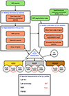 |
Fig. 2. Flowchart of the method. The input data are indicated by green boxes at the top of the figure. Black boxes refer to the different steps of the method. The corresponding sections of the paper are shown in blue. The orange boxes inside the black ones indicate the output data. The visual classification is shown by a triangle (see Sect. 3.4). The GOLD, SILVER, and BRONZE categories are illustrated by a gold, a grey, and a brown rectangle, respectively. The spectral shapes of the Lyα emission are indicated by circles, black for single- and triple-peaks and red for double-peaks. The box at the bottom presents the Lyα spectral parameters (black) and the spectral parameters measured for double-peak objects (red), detailed in Sect. 3.5. |
3.1. Building rest-frame Lyα spectra
To characterise the whole Lyα emission of each source in our parent sample, we consider a ±2000 km s−1 window around the Lyα line peak wavelength. Indeed, previous studies have shown multi-peaked Lyα lines with peak separations larger than 1000 km s−1 (Kerutt et al. 2022), even reaching values around 1800 km s−1 (Kulas et al. 2012). We use the following formula to convert wavelengths into velocities (in km s−1):
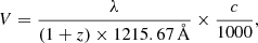 (1)
(1)
where λ is the wavelength in vacuum in Å, z is the redshift given by the Lyα wavelength in the DR2 catalogue and c is the speed of light in vacuum in m s−1 given by astropy.constants2. Before using this equation, our data are corrected using the air-to-vacuum correction function3 of the Python package MPDAF (MUSE Python Data Analysis Framework, Piqueras et al. 2019). Among the 477 sources of the parent sample, 15 have their Lyα line located near a MUSE wavelength edge, which limits the information we have to correctly process them:
-
Five objects have their Lyα line at the blue edge of the instrumental spectral range (λ ≈ 4700 Å, corresponding to z ≈ 2.8).
-
Ten of them have their Lyα line close to the AO gap (5800 Å–5966.25 Å, corresponding to redshifts between 3.8 to 3.9).
We still run the classification on these 15 objects, but we flag them as potentially missing information for reliable classification (Sect. 4.1.3).
The extracted spectra provided by the ORIGIN, ODHIN or NBEXT methods are not continuum subtracted and some sources show a stellar continuum. To accurately analyse the Lyα emission line using our classification method, we subtract the continuum following the protocol used in Kusakabe et al. (2022) adapted to the DR2 data (top left black box in Fig. 2). Briefly, the continuum spectra are estimated from spectral median filtering of the original spectra in a 100 pixel spectral window. At the end of this step, we now have a continuum-subtracted rest-frame spectrum centred on the DR2 spectroscopic redshift and over the same rest-frame wavelength window for all 477 objects of the parent sample.
3.2. Signal detection of the Lyα line
The goals of this step are, for each source, to (i) generate bootstrapped spectra to obtain their S/N spectra, (ii) run the classification method on the S/N spectra to obtain a detection spectrum, and (iii) determine the areas of signal by applying a threshold of N = 40 on the detection spectrum. This step is summarised in Fig. 2.
For each source, we generate 100 realizations of the 1D-extracted spectrum where the flux value of each pixel is randomly drawn from a normal distribution centred on its original flux value with a standard deviation given by its variance. Then, we determine their S/N spectra by dividing the flux by the square root of the variance provided by the variance datacube. For each of the one hundred S/N spectra, a peak is detected when the S/N value per pixel is above one for at least two adjacent pixels. Assuming that the noise of adjacent pixels is not correlated, the false-positive detection rate for an S/N = 2 pixel or for two adjacent pixels with an S/N = 1 is similar (∼2.3% and ∼2.5%). We choose to use a criterion of S/N ≥ 1 for at least two adjacent pixels to avoid noise spikes of 1-pixel width and to allow the detection of faint (S/N ≈ 2) Lyα emission. For each pixel of the 100 generated spectra, a value of one is assigned if this pixel belongs to a peak, otherwise, a value of zero is set. For every generated spectrum, we thus have a list of zero and one. We then sum these lists for the 100 spectra and we obtain a single list with values between zero and 100, resulting in the detection spectrum (see solid line in panel a of Fig. 3). The detection spectrum reaches 100 when a pixel belongs to a peak in 100% of the generated spectra and zero when a pixel never belongs to a peak.
Finally, to select the final areas of signal, we apply a detection threshold of N = 40 on those detection spectra (solid spectrum above the horizontal dashed green line in panel a of Fig. 3) and each pixel above this threshold is considered as real signal (shaded areas in panel a of Fig. 3). The value of N = 40 has been chosen empirically and is discussed in Appendix A.
The number of peaks of each Lyα line corresponds to the number of areas of signal.
In certain instances, an area of signal might encompass a double-peak with some flux present in the trough between the peaks. Consequently, the detection spectrum in the signal area does not fall below N = 40 (for example see Fig. 13 in Sect. 5.1). To detect such double-peaks, we conduct a flux variation analysis. This analysis consists in comparing the flux value pixel per pixel, starting from the highest value of the area of signal, which corresponds to the peak of the line. The method analyses the flux variation on both sides of the peak until reaching the edges of the area of signal. If the flux value of the pixel n + 1 is higher than the value of the pixel n, then a secondary peak is detected by the method, as illustrated in panel a of Fig. 13. This flux variation analysis is performed when there is only one area of signal detected or when, after the spatial confirmation of Lyα emission, only one area of signal remained. In the latter case, the flux variation analysis is performed and if a secondary peak is detected, this object goes through the spatial confirmation of Lyα emission phase to confirm this secondary peak.
3.3. Spatial confirmation of Lyα emission
The nature of the MUSE data allows us to investigate the spatial distribution of the Lyα peaks detected as described in the previous section (Sect. 3.2). To confirm that the emission is coming from the targeted source and to discard ‘fake’ multi-peaks caused by neighbours, we proceed to a narrow-band image inspection (see right side of Fig. 2).
For each area of signal, we extract from the MUSE cubes a 50 × 50 kpc2 narrow-band (NB) image with the same width as the area of signal, so two pixels minimum, as shown in panels b and c of Fig. 3. We then use the photutils.SourceFinder class to detect and deblend sources in our images, using a threshold of 2-σ and a minimum number of connected pixels of three for the signal search. Panels d and e of Fig. 3 show the NB images extracted from the two areas of signal A and B. We also notice the detections of SourceFinder through the segmentation maps in coloured pixels, numbered from zero. As explained in Sect. 2.3, we use reference spectra from B23 in this study. Those spectra are extracted from the MUSE datacubes using specific segmentation maps for each type of extraction (see Fig. 18 of B23). Thus, the location of the peak of the SourceFinder segmentation map (i.e. the brightest coloured pixels of SourceFinder segmentation map ‘1’ in Fig. 3) inside the reference segmentation map of B23 confirms the detection of the peak from the area of signal and has been taken into consideration during the spectral extraction. When the SourceFinder segmentation maps are located outside the reference segmentation map, they are not considered because they do not contribute to the MUSE reference spectrum.
This NB image verification is a crucial step to discard false peak detections, meaning peaks without coherent spatial counterparts. We visually inspect the NB images and the extracted spectra to determine whether the area of signal is emitting inside the segmentation map used to extract the reference spectrum in B23 or if it is noise or simply if the emission is too faint to be detected by SourceFinder with our criteria. In the example given in Fig. 3, panels d and e, we see that only one SourceFinder segmentation map is located inside the reference segmentation map. These blue segmentation maps labelled with number ‘1’ give the blue spectra on each panel and have the same shape as the reference spectrum in black. We also notice that the other SourceFinder segmentation maps (labelled ‘0’, ‘2’, and ‘3’) are located outside the reference segmentation map and their spectra are noise. The choice of using a threshold of 2-σ is discussed in Appendix A.
Out of 708 areas of signal, 89 have been discarded (i.e. 12.6%) because their SourceFinder segmentation map was outside the reference segmentation map or because nothing was detected on the NB image. This false-positive detection rate value is higher than the 2.5% false-positive detection rate expected in an ideal case, that is, when the source is isolated, without any contamination, and when the pixels are not correlated (see Sect. 3.2). This higher false-positive detection rate is thus expected given that the noise in MUSE data is correlated (Weilbacher et al. 2020; Bacon et al. 2023) and galaxies are rarely isolated in MXDF. This step enables us to classify the galaxies in three different categories following the spatial distribution of their Lyα emission, as explained in the following Sect. 3.4.
3.4. Final classification
This final step aims at providing a trustworthy classification of each Lyα line profile, taking into account the spatial distribution. We divide the parent sample into three qualitative spatial categories:
-
GOLD: when all areas of signal have only one emission located inside the reference segmentation map, and at the same spatial location. Illustration of a GOLD galaxy can be seen in panels d and e of Fig. 3 and in left panel of Fig. 4.
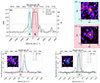
Fig. 3. ID 3240, double-peak, GOLD category. (a): Example of a detection spectrum in black obtained from the 100 realizations of the original spectrum (Sect. 3.2). The S/N spectrum of the original spectrum is plotted in dotted black. The horizontal dashed green line shows our detection threshold of N = 40 defining areas of signal. The blue A and red B shaded areas correspond to the areas of signal obtained by the crossing of the detection spectrum with the threshold line of N = 40. (b) and (c): 50 × 50 kpc2 NB images of the area of signal A and the area of signal B, respectively. The black cross represents the centre coordinates of the source. The white contours correspond to a S/N level of 2. (d) and (e): Spectra extracted from the photutils.SourceFinder segmentation maps (Sect. 3.3). The colour of each spectrum matches the NB image segmentation map colour inserted in the plot. Only the blue spectrum extracted from the blue SourceFinder segmentation map number ‘1’ contributes to the Lyα line. The reference spectrum (Sect. 2.3) in black dashed line is displayed as a reference. The dashed contours on the NB images represent the reference segmentation maps used in B23. The grey dashed contour is the segmentation map of the targeted source, the green ones correspond to other objects.
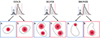
Fig. 4. Illustrations of GOLD, SILVER and BRONZE double-peaked galaxies. Left panel: Illustration of a GOLD double-peaked galaxy. The emission of each peak (red circle) is located inside the segmentation map (black contour) at the same spatial location. Middle panel: SILVER category. Each peak of the double-peaked Lyα line is coming from two different locations inside the segmentation map. Right panel: Case of a BRONZE galaxy. The blue peak (A) is emitted in a certain region and the red peak (B) is emitted in a different region of the segmentation map.
-
SILVER: when the peak emission arises from several distinct regions contained within the segmentation map, as illustrated in the middle panel of Fig. 4 and shown in Appendix B.
-
BRONZE: for double- and triple-peaked galaxies when peaks are emitted distinctly from different visual locations of the reference segmentation map. An example of this category is shown in Fig. 4, right panel.
Discarding areas of signal after spatial confirmation (Sect. 3.3) results in the declassification of double-peaks and triple-peaks into single-peaks or double-peaks. That way, the spectral classification obtained in Sect. 3.2 is different from this classification taking into account NB images. The fact that the classification changes highlights how not doing the NB verification can lead to misclassifying the line profiles. This also highlights the importance of a careful analysis of the spatial distribution of the Lyα emission to unveil the complexity of its spatial emission on top of the spectral one (see Sects. 5.1 and 5.2).
3.5. Spectral measurements on the Lyα profiles
For all categories, the following parameters are measured on the reference spectra:
-
Lyα flux (FLyα): obtained by summing the pixel flux values inside each area of signal. If the Lyα line is composed of several areas of signal, the flux of each area of signal is summed to obtain the total Lyα flux of the line. The error on the flux is determined using the variance of the spectra (i.e. the square root of the sum of the variance).
-
Lyα luminosity (LLyα): derived from the total flux of the Lyα line (FLyα, tot) and the spectroscopic redshift. The error on the Lyα luminosity is derived from the Lyα flux errors.
-
Integrated S/N: Lyα flux divided by the square root of the total variance over all the areas of signal and in between.
-
FWHM: we locate the maximum of the area of signal, we take half of this maximum value and find the two points on the spectrum corresponding to it, rounded to the nearest pixel. The error estimations of the FWHM values are determined by generating one hundred noise spectra (as explained in Sect. 3.2) for each source. Then, the standard deviation of the one hundred FWHM measurements is used to estimate the error on the FWHM. We note that the FWHM of each Lyα peak is measured.
For the double-peak objects, specific spectral measurements are determined. We refer to the peak on the left (i.e. at the bluer wavelength) as the blue peak and the one on the right (i.e. at redder wavelengths) as the red peak (but see Sect. 5.3 for discussion):
-
Blue-to-total flux ratio (B/T): the integrated flux of the blue peak is divided by the total integrated flux of the Lyα line. The error on the flux ratio is derived using the Lyα flux errors.
-
Peak separation (vsep): the velocity distance between the maxima of the blue and red peaks. The unit is km s−1. The error on the peak separation is determined by generating one hundred noise spectra for each double-peak source. Then, the standard deviation of the one hundred peak separations is taken to be the error on the peak separation.
Tables containing the measurements described above can be found in Appendix C.
3.6. Test of the method on background spectra
In order to test the reliability of the classification method on the detection of noise spikes as signal, we applied the method on 100 spectra at z = 3 and 100 at z = 6. We selected 100 random places in the continuum-subtracted MXDF cube and extracted the spectra in a two arcseconds diameter circular aperture. We selected two zones on each spectrum, one zone of ±2000 km s−1 window around the Lyα line peak wavelength as if it were emitted at z = 3, and another one as if the Lyα line peaked at z = 6. We then reproduced the exact same procedure described in Sects. 3.2 and 3.3. A summary of the results is given in Table 2.
At z = 3, over the whole selection of background spectra, 91 of them do not have any peak detected by the method. First, 52 do not pass the first part of the method (Sect. 3.2). No peaks are detected on the detection spectra. For the remaining 48 background spectra, 12 of them are discarded throughout the NB image verification (Sect. 3.3). Finally, the last step of extracting the spectra of the SourceFinder segmentation maps enables to eliminate 27 background spectra. Only six background spectra remain with a noise peak detected, one with two noise peaks. One background spectrum is clearly contaminated by a neighbouring galaxy and one last spectrum presents a clear emission line (the S/N of the peak of the line peaks above five). In total, the method detects noise peaks in 7% of the background spectra at z = 3.
At z = 6, over the whole selection of background spectra, 87 of them do not have any peak detected by the method. During the first step (Sect. 3.2), 24 spectra do not pass. Then, 16 more background spectra are discarded throughout the NB image verification. Finally, the last step of extracting the spectra of the SourceFinder segmentation maps enables to eliminate 47 background spectra. Overall, the spectra are much noisier than at z = 3. A total of 11 background spectra remain with a noise peak detected, one with two noise peaks. One background spectrum is clearly contaminated by a neighbouring galaxy. In total, the method detects noise peaks in 12% of the background spectra at z = 6.
As a result of this exercise, we estimate that around 10% of the peaks detected are spurious peaks but we decide to not make the method more selective: 10% of spurious peaks (∼76 over 760 detected peaks) is a necessary trade-off for getting an inclusive method. We keep this in mind when discussing trends in Sects. 4 and 5.
3.7. Method limitations
The method described has been designed to analyse the MUSE data (spectrum + image) and the thresholds used have been fixed following the characteristics of the MXDF. We discuss our threshold choices and characterize their impact on our results in Appendix A.
In special cases when one of the two peaks is located on the tail of the main Lyα peak, such as illustrated in Fig. 13 below, the spectral measurements done on the faintest peak contain part of the flux of the main Lyα peak. Deciphering the flux of each peak is a difficult task as we do not know the proportion of flux that is belonging to a peak or another in each pixel. In this paper, we do not attempt to deblend the peaks and we assume that each area of signal contains only one peak. Modelling such configurations could help estimate the flux ration belonging to each peak but is out of the scope of this paper.
4. Results
The first part of this section is devoted to the definition of an unbiased sample, cleaned from observational limitations. Then, we describe the physical parameter distributions of the unbiased sample regarding their Lyα line shapes. Finally, we determine the fraction of double-peaks and consider its evolution with Lyα luminosity and redshift.
4.1. Unbiased samples definitions
4.1.1. Classification of the parent sample
As explained in the previous section, we classified our galaxies in two steps. We first assign a spectral classification to ease the comparison with previous classifications that were done on spectroscopic data only (Yamada et al. 2012; Kulas et al. 2012; Hashimoto et al. 2015). We then present our final classification refined by inspecting the NB images.
The distribution of the different Lyα line shapes emergent from the signal detection of the Lyα line (Sect. 3.2), over the full parent sample, is:
-
No-peak: Lyα line is not detected, in other words, not distinguishable from the noise. Seven objects fall in this category, representing ≈1.5% of the parent sample. Three of them are Lyα absorbers (one of them, MID 103, is presented in Kusakabe et al. 2022). Six have a low confidence (ZCONF = 1) redshift B23.
-
Single-peak: 155 objects, 32.5% of the parent sample is composed of single-peaked galaxies.
-
Double-peaks: 271 have a double Lyα line. The proportion of double-peaks among the parent sample is 57%. This is the most common category.
-
Triple-peaks: 44 objects have three peaks, representing ≈9% of the parent sample.
The final step of the classification is the visual classification (Sect. 3.4) performed on each object of the parent sample taking into consideration the spatial distribution of the Lyα emission peaks (Sect. 3.3). The final classification is shown in Table 3.
Overview of the final classification.
Two objects have been added to the no-peak category, both with a ZCONF of one (which signals an unreliable redshift measurement). The spectral classification being inclusive, and therefore not fully optimized for individual cases, their NB image shows noise spikes inside the reference segmentation map resulting in extracted spectra not showing any significant peak. Spectral examples of each category are shown in Fig. 5, except for the nine ‘no-peak’ objects, shown in Appendix D. All the single-peaks, double-peaks, and triple-peaks are shown in Appendix D.
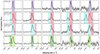 |
Fig. 5. Examples of the different spectral shape categories (Sect. 4.1), except the ‘no-peak’ category (see Appendix D). First row: spectra of single-peak galaxies. Second and third rows: spectra from sources belonging to the double-peak category, red and blue dominated spectra, respectively. Last row: spectra showing triple-peak Lyα lines. We note that the y-axis shows the flux normalized to the maximum of each line. |
4.1.2. Observational limitations
Our study aims at quantifying the diversity of LAE spectral shapes, and in particular, to give a fraction of double-peaked spectra among a population of LAEs. However, our parent sample suffers from several observational limitations, preventing us from detecting double-peaks accurately depending on their spectral characteristics (e.g. close peak separations or extreme B/T values, are harder to detect). In Sect. 4.3.1, we attempt to determine the fraction of double-peaked LAEs based on a sample cleaned from the observational biases presented below. We also do not take into consideration double-peaked BRONZE objects since the two peaks are coming from two different spatial locations, meaning the double-peak Lyα line is not produced by radiation transfer processes (see Sect. 3.4). We thus only consider the GOLD and SILVER double-peaks to determine the double-peak fraction.
Our ability to detect double peaks is expected to strongly depend on the S/N. We show on Fig. 6 the cumulative fraction of double-peaked objects with increasing S/N. Above S/N = 7, the fraction of detected double-peaks reaches a plateau of 53%, but for Lyα lines with S/N < 7, the fraction of detected double-peaks is lower (at S/N = 5, the fraction is 42%). A minimum S/N of seven is therefore required to be able to detect most of the double-peaks. We discuss below in this section the consequences of this cut on measurable B/T flux ratios.
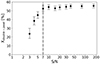 |
Fig. 6. Cumulative fraction of double-peaks with increasing S/N. The vertical dash-dotted line represents the S/N cut used to prevent missing the detection of double-peaks at lower S/N as the fraction of double-peaks drops below this value. |
Because of redshift dimming, only the brightest galaxies can be observed among the population of most distant galaxies, but thanks to the depth of the MXDF, we detect much fainter LAEs than in previous GTO surveys (B23), which allows us to investigate the evolution of Lyα properties with redshift with better statistics. We show in the left panel of Fig. 7 the Lyα luminosity distribution of our parent sample as a function of redshift. The lowest luminosity reached at z > 6.5 is LLyα = 3 × 1040 erg s−1. Applying a Lyα luminosity cut at LLyα = 3 × 1040 erg s−1 enables us to minimize the redshift dependence on the luminosity. A total of 414 LAEs match this Lyα luminosity constraint, corresponding to about 86% of the parent sample.
 |
Fig. 7. Figures illustrating the observational limitations of our sample. GOLD, SILVER, and BRONZE objects are represented by triangles, crosses, and squares symbols, respectively. Left: Lyα luminosity as a function of redshift for the parent sample. The horizontal black dash-dotted line represents the luminosity cut (LLyα = 3 × 1040 [erg s−1]) used to mitigate the redshift dependence. Middle: B/T flux ratio as a function of S/N (calculated as described in Sect. 3.5) for the whole double-peak sample. B/T ≈ 0 objects can be seen in Appendix D. They have a very small blue peak. The horizontal grey dashed line at B/T = 0.5 marks the blue-dominated versus red-dominated dividing line. The vertical black dash-dotted line represents the S/N cut (S/N = 7) made to balance the demands of being able to detect extreme B/T and keeping a representative subsample of double-peaks. The dashed lines mark boundaries of 1/(S/N) < B/T < 1–1/(S/N). Three objects have a B/T > 1 because the total flux is smaller than the flux in the blue peak because the continuum is negative between the peaks (see Appendix D). Right: Peak separation as a function of redshift for the whole double-peak sample. The horizontal black dash-dotted line represents the vsep cut (vsep = 150 km s−1) used to account for the spectral resolution of MUSE. For both the Lyα luminosity and the vsep, the observational sensitivity and spectral resolution curves are not straight lines. The ones shown in the plots are our selection limits. |
We should also keep in mind that the MUSE + VLT total efficiency rapidly declines after 7500 − 8000 Å, which makes it more challenging to detect the highest redshift objects4.
Our ability to detect B/T ranges is expected to strongly depend on the S/N (calculated as described in Sect. 3.5) of the Lyα spectra, as illustrated on the middle panel of Fig. 7. In principle, we can detect extreme B/T values only for spectra with high S/N, or, for a given S/N, we can measure B/T values in the range: 1/(S/N) < B/T < 1–1/(S/N). We choose empirically a S/N of seven, allowing the detection of double-peaks in the range 0.15 < B/T < 0.85, illustrated by a black dash-dotted vertical line in the middle panel of Fig. 7, as a compromise between being able to detect extreme B/T and keeping a statistically significant subsample. The number of galaxies having a total S/N above seven is 200, which corresponds to 46% of the parent sample.
The MUSE spectral resolution varies with wavelength, ranging from ≈150 km s−1 to ≈90 km s−1, at the blue edge (4700 Å) and the red end (9350 Å), respectively. Hence, a narrow blue peak will be less contrasted and possibly not detected at low-z while the same peak could be identified at higher redshift, where the resolution is at its maximum5. We see the smallest peak separation values evolving with redshift: when the redshift increases, the minimum peak separation decreases, from ≈150 km s−1 at z ≈ 3 to ≈90 km s−1 at z > 6 (right panel of Fig. 7). We clearly see the instrumental and redshift effects on the minimum measurable peak separation. The minimum peak separation measurable at all redshifts is vsep = 150 km s−1. The fraction of GOLD and SILVER double-peak LAEs having a Lyα peak separation above this value represents ∼76% of the double-peak sample (186/248).
4.1.3. Unbiased samples
If we take into account the observational limitations presented in the previous section (see Sect. 4.1.2), the parent sample is reduced to 214 objects. These galaxies have a Lyα luminosity above LLyα = 3 × 1040 erg s−1 and a S/N above seven. Among these 214 sources, 108 have a double-peaked Lyα line with a peak separation above 150 km s−1. These double-peaked LAEs are either GOLD or SILVER as we discarded the BRONZE ones due to the nature of their Lyα emission (Sect. 3.4). We also removed eight sources that have their Lyα line close to a spectral edge (either the AO gap or the blue edge of the MUSE spectral range, see details in Sect. 3.1), including two double-peaked objects, due to the uncertainties on their line shapes. From 214, the sample is reduced to 206 objects, 105 of them being double-peaked. The 206 remaining galaxies form the unbiased sample (U) and the 105 double-peak objects are called the inclusive unbiased double-peak sample (UDPI), as summarised in Table 4.
Overview of the samples used in this paper and the number of sources contained in each of them.
We also define a restrictive unbiased double-peak sample UDPR in which only double-peaks with a significant secondary peak are kept as double-peaks, the ones discarded being considered as single-peaks (only in this section and they are considered as double-peaks in the rest of the paper). As described at the end of Sect. 3.2, some double-peaks are contained in only one area of signal and flux variation analysis is applied on it to detect such double-peaks. This method being very basic and including no conditions on the width or the strength of the secondary peak in order to be inclusive, 145 objects in the double-peak sample (i.e. over 248, see Table 4 for reference) have been identified with this flux variation analysis. In the UDPI, this number rises to 61. In order to test the significance of the secondary peaks detected with the flux variation analysis, we implemented the following condition:
 (2)
(2)
Fpeak is the flux value at the maximum of the secondary peak, Ftrough is the flux value of the trough between the two peaks and σΔF represents the uncertainty on ΔF. Fluxes are in 10−20 erg s−1 cm−2 Å−1. We applied this condition on the UDPI and obtain a reduced number of double-peaks of 66, named UDPR. With this condition, only the obvious double-peaks remain. The discarded double-peaks are thus considered as single-peaks and stay in the unbiased sample U. An overview of the samples described above can be seen in Table 4. The inclusive and restrictive samples will be used to get an upper and a lower limit of the fraction of double-peaks, respectively (see Sect. 4.3).
4.2. Physical parameter distributions
In this section, we describe the distributions of the different physical properties measured on the Lyα lines of the unbiased sample U, presented in Fig. 8. For a better comparison, the distributions show the unbiased double-peak samples UDPI and UDPR as defined in Sect. 4.1.3 and the unbiased sample without the unbiased double-peak samples, which will be called U ∖ {UDPI} and U ∖ {UDPR} hereafter.
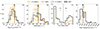 |
Fig. 8. Physical parameter distributions of the unbiased samples. (a): Logarithmic Lyα luminosity distribution. (b): FWHM distribution of the peak of the Lyα line with the strongest flux. (c): B/T distribution measured on the Lyα emission lines of the double-peaked objects. B/T = 0.5 is represented by a black dash-dotted line. The numbers written in black and orange correspond to the number of galaxies having a B/T value below 0.5 (N = 57 for UDPI and N = 51 for UDPR) and above 0.5 (N = 48 for UDPI and N = 15 for UDPR). (d): Peak separation distribution of the double-peak samples. In orange are represented the restrictive samples: U ∖ {UDPR} in dashed lines and UDPR in solid line. In black are represented the inclusive samples: U ∖ {UDPI} in dotted lines and UDPI in solid line. |
4.2.1. Lyα luminosity distribution
Panel a of Fig. 8 shows the Lyα luminosity distribution for the U ∖ {UDP} and UDP for both the restrictive (in orange) and inclusive (in black) samples. The Lyα luminosity of the samples ranges from log(LLyα [erg s−1]) = 40.57 to 43.03. Thanks to the unprecedented depth of the MXDF data, our sample reaches one order of magnitude lower in terms of Lyα luminosity compared to the LAE sample of Kerutt et al. (2022) containing MUSE-Wide and MUSE-Deep (MOSAIC and UDF-10) LAEs. The two samples U ∖ {UDPI} (dotted black histogram) and U ∖ {UDPR} (dashed orange histogram) show a similar distribution, with more objects in the U ∖ {UDPR} as the number of double-peaks in UDPR is smaller than in UDPI. For the unbiased double-peak samples, UDPR in solid orange and UDPI in solid black, the distributions also show similarities. They span over the same luminosity range. The mean value of UDPR is log(LLyα [erg s−1]) = 41.83 while the mean value of UDPI is log(LLyα [erg s−1]) = 41.78. Despite the condition applied to get the restrictive unbiased double-peak sample UDPR, the Lyα luminosity distribution of UDPR and UDPI show similar trends. Due to the strong constraint on Lyα luminosity applied on the parent sample to obtain the unbiased samples, the distributions of the U ∖ {UDP} and the UDP, for both the inclusive and restrictive samples, are very similar, especially their mean Lyα luminosity. Nevertheless, the luminosity distributions of the U ∖ {UDPI} and the U ∖ {UDPR} samples tend to slightly peak at a fainter luminosity than their respective unbiased double-peak samples UDPI and UDPR.
4.2.2. Full width at half maximum distribution
The FWHM is broadened by radiation transfer effects and has been proposed as a proxy for the peak shift of the Lyα line that can be used to recover systemic redshift when only Lyα is detected (Verhamme et al. 2018). Panel b of Fig. 8 displays the FWHM distributions of the peak of the Lyα line with the strongest flux for the different unbiased samples. The two distributions U ∖ {UDPI} and U ∖ {UDPR} peak between 200 and 300 km s−1 while the two double-peak samples, UDPI and UDPR, peak between 300 and 400 km s−1. Double-peaked Lyα lines tend to have wider profiles than the other Lyα lines of the unbiased samples. The mean FWHM values of UDPI (332 ± 9 km s−1) and UDPR (347 ± 11 km s−1) are similar, taking into account the errors. These measurements are consistent with other results obtained for LAEs observed with MUSE (Kerutt et al. 2022; Leclercq et al. 2017).
4.2.3. Blue-to-total flux ratio distribution
Concerning the unbiased double-peak samples only, we measure the B/T flux ratio (see Sect. 3.5) where the distributions of UDPI and UDPR are shown in panel c of Fig. 8. For the inclusive unbiased double-peak sample UDPI, a bit more than half of the sample (54%, 57/105) is red-peak dominated (i.e. B/T < 0.5) while the other half is blue-peak dominated. We observe 82 objects with extreme B/T values as defined in Blaizot et al. (2023), that is, between 0 < B/T ≤ 0.1 and 0.6 ≤ B/T < 1, and 23 objects between B/T = [0.1−0.6]. We use the term ‘extreme’ for B/T > 0.6 because of the rareness of such objects in the literature. We show in the middle panel of Fig. 7 the B/T flux ratio versus the S/N. The extreme B/T values have high S/N, which seems to indicate that the shape of this distribution is not due to noise. This distribution is surprising since so far, very few blue-peak-dominated galaxies have been reported in the literature, from LAEs (Kulas et al. 2012; Wofford et al. 2013; Erb et al. 2014; Trainor et al. 2015; Izotov et al. 2020; Kerutt et al. 2022; Furtak et al. 2022; Marques-Chaves et al. 2022; Mukherjee et al. 2023) and for other types of sources such as AGNs or extended Lyα nebulae (Martin et al. 2015; Vanzella et al. 2017; Ao et al. 2020; Daddi et al. 2021; Li et al. 2022). Blue-dominated spectra are also rare according to simulations, as described in Blaizot et al. (2023). Indeed, they found that less than 20% of the Lyα lines are blue-dominated in their work. We discuss our high B/T values in Sect. 5.3. For the restrictive unbiased double-peak sample UDPR, we observe a drastic decrease of the number of blue peak dominated: from 48 for UDPI to 15 for UDPR. The fraction of the sample that is red-peak dominated is 23%, which is close to the fraction measured in Blaizot et al. (2023). For B/T flux ratios between 0.1 and 0.6, the distributions of UDPR and UDPI remain the same. For extreme B/T values, the distributions are different, UDPR having much less of this kind of values. This difference is explained by the condition applied to get UDPR, as explained in Sect. 4.1.3. We discarded double-peaks with a non significant secondary peak compared to the trough between the two peaks. By definition, double-peaked Lyα lines with extreme B/T values tend to have more non significant secondary peaks compared to the double-peaks with intermediate B/T values ([0.1−0.6]).
4.2.4. Peak separation distribution
The peak separation distribution of the unbiased double-peak samples (Fig. 8, panel d) ranges from 150 km s−1 to almost 1600 km s−1. The mean value of UDPI (in black) is 447 ± 22 km s−1 and the mean value of UDPR (in orange) is 534 ± 28 km s−1, which is coherent with the mean peak separation measured by Kerutt et al. (2022) for MUSE-Wide and MUSE-Deep LAEs (481 ± 244 km s−1), z ≈ 2.2 LAEs from Hashimoto et al. (2015) (500 ± 56 km s−1) or even z ≈ 2 galaxies from Matthee et al. (2021) (500 km s−1). We notice that the restrictive sample (UDPR) has Lyα double-peaks with wider peak separations than the inclusive sample. A drop of the number of peak separations below 400 km s−1 is observed for the UDPR sample compared to the UDPI one. This is explained by the condition (described in Sect. 4.1.3) applied on the double-peaks detected with the flux variation analysis. This flux variation analysis is applied inside one area of signal (see Sect. 3.2), which results most of the time on the detection of close by peaks. Thus, Lyα double-peaks with small peak separations (< 400 km s−1) have more non significant secondary peaks than Lyα double-peaks with bigger peak separations. The distributions of both UDPR and UDPI are similar above 700 km s−1 with a severe drop above 800 km s−1, similarly to Kulas et al. (2012), Trainor et al. (2015) and Kerutt et al. (2022). The results are consistent with the overall literature, as we can see in Fig. 9 that compiles the peak separation measurements and redshifts of double-peaked Lyα lines reported in the literature.
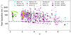 |
Fig. 9. Peak separation plotted against the redshift for our double-peak sample and for several studies (Kulas et al. 2012; Yamada et al. 2012; Hashimoto et al. 2015; Matthee et al. 2018; Songaila et al. 2018; Bosman et al. 2020; Meyer et al. 2021; Naidu et al. 2022). Our double-peak sample represented in purple shows three different symbols for the three categories GOLD (triangle), SILVER (cross), and BRONZE (square). A horizontal black dash-dotted line at 150 km s−1 represents the peak separation threshold made in Sect. 4.1.2 to obtain the fraction of double-peaks. The peak separations are in discrete lines due to the fact that the minimal peak separation measured is two spectral bins and depends on redshift. |
4.3. Towards a determination of a double-peak fraction
4.3.1. Fractions of double-peak
The double-peak fraction (XDP), for the inclusive and restrictive samples are:
 (3)
(3)
and
 (4)
(4)
respectively.
Our fraction of double-peaked galaxies XDP I is an upper limit given the probability of spurious detections of 10% (see Sect. 3.6), while XDP R gives a lower limit due to the restrictive nature of the sample UDPR. This range of the fraction of double-peaks (32%≤XDP ≤ 51%) is consistent with most of the fractions reported in the literature. Indeed, Kulas et al. (2012) and Sobral et al. (2018) find fractions of 30% and 25%, for z = 2 − 3 LAEs, Cao et al. (2020) find an average fraction of 20% for lensed galaxies and Kerutt et al. (2022) find 33% for the MUSE-Wide and MUSE-Deep LAEs. Moreover, Trainor et al. (2015) with a fraction of 40% at redshift ∼2.7 or Yamada et al. (2012) finding 50% of double-peaks for their LAEs at z = 3.1.
It is important to note that the fractions given in the literature are not corrected for observational biases, which could lead to an underestimation of the double-peak fraction. Additionally, double-peaks in the literature are detected either visually (Yamada et al. 2012; Kerutt et al. 2022) or with an algorithm (Trainor et al. 2015) completed by a visual inspection only on the spectra (Kulas et al. 2012), the spatial data being unavailable for most studies.
4.3.2. Fraction of double-peak evolution with Lyα luminosity
To investigate if the fraction of double-peaks varies with luminosity, we divide our unbiased samples into four Lyα luminosity bins with the same number of objects. Figure 10 shows XDP I and XDP R for each of the four luminosity bins. The fraction of double-peaks from the inclusive sample evolves from around 34% for the faintest luminosities to nearly 60% for the brightest bin (41.7 < log(LLyα [erg s−1]) < 43). Concerning the evolution of the fraction of double-peaks for the restrictive sample, we observe a similar trend as for the inclusive sample, meaning an increase towards the brighter luminosities, except for the brightest bin in which XDP R is smaller than in the previous bin. The fraction evolves from 17% to 37% with a peak at 43% for the third bin (41.4 < log(LLyα [erg s−1]) < 41.7). As both samples are the lower and upper limits of our study, we might consider the real fraction of double-peaks per bin of Lyα luminosity between the two trends shown in Fig. 10 delimited by the grey area. Moreover, as the trends remain the same whatever the restrictions applied on the double-peak sample, they are robust. Brighter galaxies seem to have more double-peaked Lyα lines, as seen in the Lensed Lyman-Alpha MUSE Arcs Sample of Claeyssens et al. (in prep.). However, since it is easier to detect double-peaks for bright galaxies, this trend may still be due to observational biases. We explore the bright end of the MUSE GTO samples in forthcoming work by applying our classification method to wider surveys. The evolution of the fraction of double-peaks per spatial category (GOLD and SILVER), in the unbiased sample, is described in Appendix E.
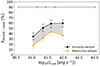 |
Fig. 10. Fraction of double-peaked LAEs plotted against the logarithmic Lyα luminosity. The unbiased sample U has been divided into four luminosity bins with the same number of objects (51 or 52). The fraction of double-peaks has been derived in each bin for both UDPI and UDPR. The results are positioned at the median Lyα luminosity of each bin. The fractions of inclusive double-peaks are represented in black colour. The XDP R of the restrictive sample are in orange. The horizontal black line at the top of the figure shows the size of each Lyα luminosity bin. |
Blaizot et al. (2023) find an anti correlation between the Lyα luminosity and the B/T flux ratio of the Lyα line in their simulations. The higher the luminosity (i.e. face-on galaxy), the lower the B/T is. In the top panel of Fig. 11, we plot the B/T distribution for the inclusive unbiased double-peak sample (UDPI) split into two luminosity bins with the same number of objects. The sample is cut at LLyα = 3.7 × 1041 erg s−1. We notice that the bright subsample (grey histogram in top panel of Fig. 11) populates more the red peak dominated regime (i.e. B/T < 0.5) than the blue peak dominated one (i.e. B/T > 0.5). On the contrary, the faint subsample (black histogram) is more dominant in the intermediate B/T range and high B/T range. Our results are in line with what Blaizot et al. (2023) find in their simulations. The lower panel of Fig. 11 shows the same plot but for the restrictive unbiased double-peak sample (UDPR) and a Lyα luminosity cut at cut at LLyα = 3.9 × 1041 erg s−1. The bright subsample (orange histogram) shows more clearly a strong presence at the lower B/T values and a small number of objects at B/T > 0.5 compared to UDPI. The presence of the faint subsample at high B/T values is comparable with the simulations in Blaizot et al. (2023). Nevertheless, an important number of faint galaxies also have smaller values of B/T.
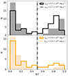 |
Fig. 11. B/T flux ratio distributions shown for bright and faint galaxies. Top panel: B/T flux ratio distributions of the inclusive unbiased double-peak sample (UDPI) divided into two Lyα luminosity bins with the same number of objects (53 and 52). The faint subsample (LLyα < 3.7 × 1041 erg s−1) is in black and the bright one (LLyα > 3.7 × 1041 erg s−1) is in grey. Bottom panel: B/T flux ratio distributions of the restrictive unbiased double-peak sample (UDPR) divided into two Lyα luminosity bins with the same number of objects (33 and 33). The faint subsample (LLyα < 3.9 × 1041 erg s−1) is in stepped orange and the bright one (LLyα > 3.9 × 1041 erg s−1) is in orange. B/T = 0.5 is represented by a black dash-dotted line in both panels. |
4.3.3. Fraction of double-peak evolution with redshift
According to theoretical predictions, the IGM attenuation increases with redshift, absorbing the blue part of the Lyα emission (Laursen et al. 2011; Garel et al. 2021). Hayes et al. (2021) indeed find for stacked spectra that the fraction of flux bluewards of the main (red) peak decreases with redshift. This trend has also been reproduced by Kramarenko et al. (2024) by stacking MUSE-Wide LAE spectra. We therefore expect the double-peak fraction to decrease with redshift.
Figure 12 shows the evolution of the fraction of double-peaks with redshift for the inclusive (restrictive) sample in black (orange): we report a global decrease from  (
( ) at z ∼ 3 down to
  (
( ) at z > 5.5, but above z = 4, the data are compatible with a plateau around 40% (20%). Since we report on Fig. 10 a strong evolution of the fraction of double-peaks with luminosity, these plateaux might be caused by the high mean luminosity (represented by stars on Fig. 12) in the last three bins, artificially raising the fraction of double-peaks. At low redshift (z < 3.5), we see an interesting increase in the double-peak fraction. If this trend is confirmed with more data, it could indicate an intrinsic evolution of the LAE population towards cosmic noon. If such a possible evolution is confirmed, it could make less pertinent the use of the double-peak fraction to probe the opacity of the IGM at this redshift range.
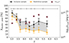 |
Fig. 12. Fractions of double-peaked LAEs plotted against the redshift. The unbiased sample has been divided into eight redshift bins with the same number of objects (25 or 26). The fraction of double-peaks has been derived in each bin. The results are positioned at the median redshift of each bin. The fractions of inclusive double-peaks are represented in black colour. The XDP of restrictive objects are in orange. The horizontal black line at the top of the figure shows the size of each redshift bin. The black stars surrounded in red represent the mean Lyα luminosity of each bin. |
The two evolutions of the fraction of double-peaks, one inclusive and the other one restrictive, give us the lower and upper limits of the XDP range (shaded area on Fig. 12) our sample truly have. Additionally, the trend of the evolution of the fraction of double-peaks is conserved regardless of the way the double-peaks are spectrally detected. Our classification is robust. The evolution of the fraction of double-peaks with redshift per spatial category (GOLD and SILVER), in the unbiased sample, is discussed in Appendix E.
5. Discussion
5.1. Contaminants to the multi-peak sample
In this subsection, we describe the physical interpretation of the BRONZE category defined in Sect. 3.4. As a recap, 11 objects belong to the BRONZE category: ten double-peaks and one triple-peak (Sect. 4.1.1).
Figure 13 illustrates an interesting case where the NB images show a well centred Lyα emission (b1) plus another small compact emission offset from the centre of the central source. This compact emission, named b2 in panels b–d is significantly detected on the NB image B and not detected on the NB image A. Interestingly, there is no HST counterpart (panel d of Fig. 13) and no detection in the MUSE DR2 catalogue. The spectra extracted from b1 and b2 apertures show that b2 contributes to most of the red peak of the Lyα line. We interpret this compact emission b2 as a satellite. Among these ten double-peaks, nine of them present a similar configuration like in Fig. 13. In the last BRONZE double-peaked LAE, the blue peak is artificially created by the Lyα halo of a neighbouring galaxy, as illustrated in Fig. 14. Panels b and d show that peak A is emitted by a neighbouring galaxy (ID 8455) that is included in the reference segmentation map of our targeted galaxy. Follow-up observations in the infrared are necessary to confirm the hypothesis of the satellites but it may be challenging, given the fact that our targets are very faint.
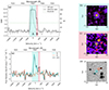 |
Fig. 13. ID 399, double-peak, BRONZE category. Example of a LAE surrounded by a satellite discovered thanks to our method. (a)–(c): Same as Fig. 3. The cyan circle b1 and the orange circle b2 represent the apertures used to extract two spectra at the indicated locations. The size of the circles represent a 0.5″ diameter aperture. (d): 50 × 50 kpc2 HST F125W image with the two locations of the extraction (cyan and orange circles). (e): Spectra extracted from the two circles. The orange dash-dotted line corresponds to the spectrum extracted at the position of b2. The spectrum extracted from b1 is shown as a cyan dashed line. The black line is the summed spectrum of the blue and orange spectra. The spectrum extracted at the position b2, that is the position of the satellite, contributes mainly to the peak B. |
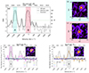 |
Fig. 14. ID 8439, double-peak, BRONZE category. Same as Fig. 3. Peaks A and B come from two different spatial locations. Peak A is the Lyα emission of the halo of ID 8455 (contained in the reference segmentation map of ID 8439). Peak B is the Lyα emission coming from the targeted galaxy. |
The BRONZE category contains galaxies showing a double-peak Lyα profile on the spectra but not on the NB images of each peak. Indeed, the NB image of only one of the peaks contains a small compact emission offset from the centre of the galaxy (as shown in panels b and c of Fig. 13), discarding the fact that these Lyα lines originate from radiative transfer processes. We call the ten double-peaked BRONZE sources fake double-peaks. The fraction of fake double-peaks among the total number of double-peaked galaxies (248, Sect. 4.1.1), XFDP, is:
 (5)
(5)
Spectral only classification would consider these objects as double-peaked LAEs whereas they are not. As a note, even galaxies that are spatially unresolved in MUSE may have multiple unresolved spatial components associated with different spectral components. As such, the distinction between ‘fake’ and ‘real’ multi-peak LAEs may be blurry. Thus, XFDP represents a lower limit.
5.2. Galaxy pairs identification and prospects
Interacting galaxies are not limited to the BRONZE category, as we explain below. This BRONZE category contains only galaxies that are in interaction with other objects in a very small area, meaning inside the reference segmentation map used in DR2 (see Sect. 3.3). These objects do not show a particular trend in their B/T values.
The SILVER category (see Sect. 3.4 for details) contains objects for which more than one SourceFinder detection is located inside the reference segmentation map. These detections correspond sometimes to well-identified objects in the MUSE DR2 catalogues (10/38), but sometimes not (28/38) as illustrated in Fig. B.1. Nevertheless, the SILVER galaxies are interpreted as being in interaction since very close by clumps are visible. With the data we have in hand, we are not yet able to identify if the SILVER objects are coming from two clumps of the same source, or from two different objects. Additional data detecting other lines could help in this differentiation.
Finally, visually inspecting the NB images enabled us to discover complex systems. We discovered 40 galaxies lying in pairs (20 pairs), meaning two galaxies at a similar redshift and very close (less than 25 kpc, see Fig. 15 for example). Among those pairs, ten galaxies are SILVER. Moreover, three other systems have been identified. In all cases, three galaxies of similar redshifts are located within a distance of 25 kpc. We call them triplet systems. One if the triplet system is shown in Fig. 16. The pairs and triplet systems are flagged in Appendix C. Given their proximity, all these systems are consistent with interacting systems.
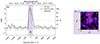 |
Fig. 15. ID 7817, single-peak, GOLD category. Example of a pair of galaxies. The galaxy ID 8271 has the same redshift as ID 7817 (z ≈ 4.14). |
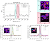 |
Fig. 16. ID 412, double-peak, GOLD category. Same as Fig. 3. Example of a triplet system of galaxies (ID 412, 6698 and 8355) at z ≈ 4.13. Interestingly, in panel e, two galaxies have a similar red-dominated double-peaked Lyα line profile while the third one, labelled 1, shows a blue-dominated double-peak line. |
As a summary, in our parent sample, the BRONZE objects, the SILVER ones, the 40 galaxies in pairs as well as the nine galaxies in triplet systems are interpreted as being in interaction. The fraction of such systems, called Xinteraction, is:
 (6)
(6)
Interacting galaxies are usually discarded from Lyα studies although they represent a significant fraction of our sample. A more detailed analysis of the effect of the environment on the spectral diversity of LAEs is beyond the scope of this paper. The pairs and the three triplet systems will be the subject of another study (Vitte et al., in prep.).
5.3. Lack of systemic redshift
The Lyα line is resonant, and radiative transfer effects can result in a double-peaked profile, with peaks on each side of the resonance frequency (Neufeld & McKee 1990; Dijkstra et al. 2006; Dijkstra 2017). Based on this assumption, methods have been developed to retrieve the systemic redshift of a galaxy using the Lyα line shape (Verhamme et al. 2018), or the escape fraction of the ionizing radiation using the Lyα peak separation (Verhamme et al. 2015). Moreover, the B/T measurements can provide information about the gas kinematic configuration (inflows/outflows), as demonstrated in Blaizot et al. (2023).
Throughout this study, we call ‘blue peak’ the peak with the shortest wavelength and ‘red peak’ the one at the longer wavelength, although we do not know the systemic redshift (zsys) of most of our galaxies. Our population of double-peaked LAEs may differ from what is usually called a double-peak in the sense that the blue (red) peak might not be bluer (redder) than the resonant frequency of the central object. In the same way, single-peaked lines are by default presumed being on the red side of the resonant frequency, since we do not know their systemic redshift. But this assumption for single-peaked lines does not impact the results presented in this paper.
In this section, we investigate the spectral parameters of a subsample of galaxies with known systemic redshift whose spectra are shown in Appendix F. Fifteen objects have a secure systemic redshift measured from nebular lines detected in their MUSE spectra. One of those (ID 53), was studied in detail in Matthee et al. (2022) and its systemic redshift is well constrained. Five others were studied in Kusakabe et al. (2022) (MID 106, MID 118, MID 149, MID 6700 and MID 7089). One last (ID 6666) has its redshift measured by the K-band Multi Object Spectrograph (VLT/KMOS) in Boogaard et al. (2021). Eight sources of this subsample with systemic redshift are double-peaked, three are single-peaked and the last four are triple-peaked. They all belong in the GOLD category. The luminosities of those galaxies do not go lower than log(LLyα [erg s−1]) = 40 but they populate the bright end of the distribution with a mean logarithmic Lyα luminosity of 42.25 (panel a). This is expected as fainter galaxies usually only have their Lyα line detected. Most of the objects have a FWHM of the peak of the Lyα line with the strongest flux within the range 250−550 km s−1. Only one galaxy has a small FWHM of 129 km s−1. Only one galaxy has a B/T above 0.5 and it is as well the only one having both the blue and red peaks on the red side of the systemic (see ID 263 in Appendix F and Fig. 17). Four of the double-peaks have a small B/T (less than 0.1). The three last galaxies of this subsample have a B/T that does not exceed 0.4. Concerning the peak separation distribution of the double-peaked LAEs having a systemic redshift, the distribution is concentrated in a small range, between 400 and 800 km s−1. The mean peak separation is 578 km s−1. This is 1.3 times higher than the mean value of the unbiased double-peak sample (447 ± 29 km s−1). Figure 17 shows a graphical summary of peak velocities for the eight double-peaked galaxies having a systemic redshift. The mean values of our sample are:
-
Blue peak: −333 ± 47 km s−1.
-
Trough: −70 ± 74 km s−1.
-
Red peak: 253 ± 79 km s−1.
Our sample has a similar mean red peak shift than the LAE sample of Trainor et al. (2015) (200 km s−1) although their sample is NB-selected whereas our survey is blind. It has on average broader peak separations than the Green Peas studied in Orlitová et al. (2018), which have a mean peak separation of ±400 km s−1 and some are known to leak LyC. However, compared to the Lyman-break galaxies (LBGs) of Kulas et al. (2012), our sample has narrower peak separations. The mean peak separation of the LBGs is 770 km s−1. As LBGs are more massive galaxies (1010 − 11 M⊙, Carilli et al. 2008) than LAEs (108 − 9 M⊙, Ouchi et al. 2020), this might explain the large peak separations measured by Kulas et al. (2012), as, on average, the Lyα photons have to scatter more through the LBGs to escape. Looking at the position of the trough, we notice it is mostly located bluewards with respect to the systemic velocity. Together with the red dominated characteristic, this is expected in the framework of radiation transfer through an outflowing medium (Fig. 14 in Verhamme et al. 2006). Orlitová et al. (2018) have a mean position of the trough centred on the systemic velocity while Kulas et al. (2012) have a mean trough at 143 km s−1.
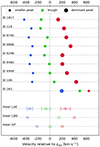 |
Fig. 17. Velocities of every peak and trough for the double-peaked galaxies having a systemic redshift (Sect. 5.3). Each line corresponds to a source, where the blue (red) circle shows the bluer (redder) peak and the green square indicates the position of the trough. The larger circle represents the peak with the highest flux. The first line of the bottom part of the figure shows the mean positions of the trough and the blue and red peaks of the objects shown above (without taking into account ID 263). The mean LBG and mean Green Pea (GP) are drawn from the literature, Kulas et al. (2012) and Orlitová et al. (2018), respectively. |
Only one galaxy has the bluer peak dominant (ID 263, B/T = 0.98, Fig. 17). This is also the only galaxy with the two peaks located on the red side of the systemic redshift. Such a configuration has already been observed in Kulas et al. (2012) and Trainor et al. (2015). In this case, the double-peak profile does not emerge from radiative transfer processes, and thus it is not possible to retrieve the escape fraction of ionizing radiation from the peak separation, nor to interpret the bluer peak dominance as inflowing gas (Zheng & Miralda-Escudé 2002; Dijkstra et al. 2006; Verhamme et al. 2006; Blaizot et al. 2023). To be able to retrieve these parameters, we need to know the systemic redshift as highlighted in Blaizot et al. (2023). A dedicated VLT/KMOS proposal (113.2682.001(A), PI: Vitte) has been approved and will observe during Period 113 a total of 21 galaxies from MUSE-Deep (Bacon et al. 2023; Inami et al. 2017) and MUSE-Wide (Urrutia et al. 2019) fields to precisely measure their systemic redshift.
6. Summary and conclusion
In this paper, we present the diversity of the Lyα line shapes among a population of MUSE LAEs. We constructed a parent sample of 477 redshift-selected (z = 2.87 − 6.64) sources from a blind, extremely deep MUSE GTO survey, the MXDF (up to 140 hours of integration time; Bacon et al. 2023). The main results of our work are summarised as follows:
-
We developed a method to detect and characterise the Lyα emission lines in both spectral and spatial dimensions (Sect. 3).
-
The Lyα lines from the sources of the parent sample are quantitatively classified into four different spectral categories: no-peak (9), single-peak (198), double-peak (248), and triple-peak (22); see Sect. 4.1.1 and Fig. 5.
-
Our analysis of the spatial distribution of the Lyα peaks enabled us to divide the parent sample into three different categories: GOLD, SILVER, and BRONZE (Sect. 3.4 and Fig. 4). An object is classified as GOLD if all the peaks originate from the same spatial location. When the peak emission arises from several distinct regions contained within the reference segmentation map, the object is thus classified as a SILVER object. Finally, for double- and triple-peaks, an object can be classified BRONZE. In that case, each peak has an emission coming from a distinct spatial location, which means the peaks are coming from different sources. Among the 248 double-peaks, 238 are GOLD or SILVER objects (i.e. considered as double-peaks coming from radiative transfer processes). The last ten cannot be considered as such given their spatial distribution (i.e. BRONZE objects).
-
We identified several observational limitations: the fainter the source, the harder it is to detect multi-peaks; the minimum peak separation detectable varies with redshift; the detectable range of B/T ratios depends on the S/N (see Sect. 4.1.2). Taking into account these limitations, we built an unbiased sample of 206 galaxies, with Lyα luminosities of above 3 × 1040 erg s−1, peak separations of larger than 150 km s−1 and S/N of above 7.
-
For each object, we measured spectral properties, such as the Lyα flux, the Lyα luminosity, the S/N, and the FWHM, and we also measured the peak separation and blue-to-total flux ratio (B/T) for double-peaks. Our study reaches fainter luminosities (log(LLyα [erg s−1]) = 39.5) thanks to the depth of our data. Our derived FWHM and the peak separation values from the unbiased sample are comparable to other studies in the literature, whereas the B/T distribution shows an important fraction of blue-dominated spectra (Sect. 4.2.3).
-
We found a fraction of double-peaks XDP oscillating between 32% and 51% within two double-peak unbiased samples, one restrictive – giving the lower limit – and one inclusive – giving the upper limit (Sect. 4.3.1). This fraction seems to evolve dependently with the Lyα luminosity (Sect. 4.3.2).
-
This fraction of double-peaks shows a global decrease with redshift, stagnating at high redshift (Sect. 4.3.3). This plateau might be due to the high mean Lyα luminosity of each redshift bin, knowing that brighter galaxies seem to have more double-peaked Lyα lines. Nevertheless, if the increase in the XDP at lower redshift is confirmed with more data, the use of the double-peaked fraction to probe the opacity of the IGM becomes less pertinent.
-
The double-peaks identified by the method are not necessarily double-peaks originating from radiative transfer (BRONZE category, see Sect. 5.1), but could come from satellites. Indeed, the NB images of the Lyα peaks detected by the method show a wide variety of environments for galaxies. This method unveils the detection of satellites (companions) of main targeted galaxies and also interactions between galaxies (pairs, triplet systems) independently of the spectral category (Sect. 5.2). A detailed characterisation of the environment of the pairs and triplet galaxies studied here will be the subject of an upcoming study (Vitte et al., in prep.).
-
Peak separation and B/T flux ratio have a physical meaning (i.e. they are tracers of the escape of ionizing photons for peak separation of < 400 km s−1 and infalling gas for B/T > 0.5) only if the systemic velocity is located between the blue and the red peaks. We were able to measure a systemic redshift for a subsample of 15 galaxies from the MUSE data (Sect. 5.3). The only blue dominant peak with a systemic redshift has its two peaks located on the red side of the systemic redshift. This spectrum thus cannot be considered as tracing infalling gas. More systemic redshift measurements are needed in order to interpret our distributions further. A recently approved VLT/KMOS proposal (113.2682, PI: Vitte, 60 h) will allow us to increase this subsample of systemic redshifts.
The aim of this paper is to describe the method we developed to classify Lyα emission lines from high-redshift galaxies and its application to a blind sample from MUSE GTO surveys. A more detailed study of the completeness will be the scope of future work. We plan to apply the method developed and used for this work to other data sets, which will give us a more general view of the fraction of double-peaks among LAEs and how it evolves with redshift. We will also use existing data (e.g. FRESCO, JADES, Oesch et al. 2023; Eisenstein et al. 2023, respectively) and obtain new data (VLT/KMOS proposal, 113.2682, PI: Vitte, 60 h) obtain the systemic redshift of more galaxies of the MXDF in order to constrain the distributions we found during this study.
The infrared instruments such as VLT/KMOS and JWST/NIRSpec allow us to perform a multi-wavelength study to explore the possible physical peculiarities of the different categories of LAEs. In the longer term, this work can be pursued at lower redshift – for example down to z ≈ 2 – thanks to the upcoming BlueMUSE (Richard et al. 2019), allowing us to unveil the evolution of the diversity of the LAE population with time, over three more gigayears of galaxy evolution.
Data availability
Figures of Appendices D and F are available at https://zenodo.org/records/14235906
Full Tables C.1–C.3 are available at the CDS via anonymous ftp to cdsarc.cds.unistra.fr (130.79.128.5) or via https://cdsarc.cds.unistra.fr/viz-bin/cat/J/A+A/694/A100
Acknowledgments
EV and AV acknowledges the support from the SNF grants PP00P2 176808 and 211023. HK acknowledges support from Japan Society for the Promotion of Science (JSPS) Overseas Research Fellowship as well as JSPS Research Fellowships for Young Scientists. JP acknowledges funding by the Deutsche Forschungsgemeinschaft, Grant Wi 1369/31-1. This work is based on observations taken by VLT, which is operated by European Southern Observatory. This research made use of ASTROPY, which is a community-developed core Python package for Astronomy (Astropy Collaboration 2013, 2018, 2022), and other software and packages: MPDAF (Piqueras et al. 2019), PHOTUTILS (Bradley 2023), NUMPY (van der Walt et al. 2011), SCIPY (Virtanen et al. 2020). The plots in this paper were created using MATPLOTLIB (Hunter 2007).
References
- Ao, Y., Zheng, Z., Henkel, C., et al. 2020, Nat. Astron., 4, 670 [NASA ADS] [CrossRef] [Google Scholar]
- Astropy Collaboration (Robitaille, T. P., et al.) 2013, A&A, 558, A33 [NASA ADS] [CrossRef] [EDP Sciences] [Google Scholar]
- Astropy Collaboration (Price-Whelan, A. M., et al.) 2018, AJ, 156, 123 [Google Scholar]
- Astropy Collaboration (Price-Whelan, A. M., et al.) 2022, ApJ, 935, 167 [NASA ADS] [CrossRef] [Google Scholar]
- Bacher, R. 2017, Ph.D. Thesis [Google Scholar]
- Bacon, R., Accardo, M., Adjali, L., et al. 2010, in Ground-based and Airborne Instrumentation for Astronomy III, eds. I. S. McLean, S. K. Ramsay, & H. Takami, SPIE Conf. Ser., 7735, 773508 [Google Scholar]
- Bacon, R., Conseil, S., Mary, D., et al. 2017, A&A, 608, A1 [NASA ADS] [CrossRef] [EDP Sciences] [Google Scholar]
- Bacon, R., Brinchmann, J., Conseil, S., et al. 2023, A&A, 670, A4 [NASA ADS] [CrossRef] [EDP Sciences] [Google Scholar]
- Blaizot, J., Garel, T., Verhamme, A., et al. 2023, MNRAS, 523, 3749 [NASA ADS] [CrossRef] [Google Scholar]
- Boogaard, L. A., Bouwens, R. J., Riechers, D., et al. 2021, ApJ, 916, 12 [NASA ADS] [CrossRef] [Google Scholar]
- Bosman, S. E. I., Kakiichi, K., Meyer, R. A., et al. 2020, ApJ, 896, 49 [Google Scholar]
- Bradley, L. 2023, https://doi.org/10.5281/zenodo.7946442 [Google Scholar]
- Bunker, A. J., Saxena, A., Cameron, A. J., et al. 2023, A&A, 677, A88 [NASA ADS] [CrossRef] [EDP Sciences] [Google Scholar]
- Cao, X., Li, R., Shu, Y., et al. 2020, MNRAS, 499, 3610 [NASA ADS] [CrossRef] [Google Scholar]
- Carilli, C. L., Lee, N., Capak, P., et al. 2008, ApJ, 689, 883 [NASA ADS] [CrossRef] [Google Scholar]
- Daddi, E., Valentino, F., Rich, R. M., et al. 2021, A&A, 649, A78 [NASA ADS] [CrossRef] [EDP Sciences] [Google Scholar]
- Dijkstra, M. 2017, ArXiv e-prints [arXiv:1704.03416] [Google Scholar]
- Dijkstra, M., Haiman, Z., & Spaans, M. 2006, ApJ, 649, 14 [NASA ADS] [CrossRef] [Google Scholar]
- Eisenstein, D. J., Willott, C., Alberts, S., et al. 2023, ApJS, submitted [arXiv:2306.02465] [Google Scholar]
- Erb, D. K., Steidel, C. C., Trainor, R. F., et al. 2014, ApJ, 795, 33 [Google Scholar]
- Flury, S. R., Jaskot, A. E., Ferguson, H. C., et al. 2022, ApJS, 260, 1 [NASA ADS] [CrossRef] [Google Scholar]
- Furtak, L. J., Plat, A., Zitrin, A., et al. 2022, MNRAS, 516, 1373 [NASA ADS] [CrossRef] [Google Scholar]
- Garel, T., Blaizot, J., Rosdahl, J., et al. 2021, MNRAS, 504, 1902 [NASA ADS] [CrossRef] [Google Scholar]
- Green, J. C., Froning, C. S., Osterman, S., et al. 2012, ApJ, 744, 60 [NASA ADS] [CrossRef] [Google Scholar]
- Hashimoto, T., Verhamme, A., Ouchi, M., et al. 2015, ApJ, 812, 157 [Google Scholar]
- Hayes, M. J., Runnholm, A., Gronke, M., & Scarlata, C. 2021, ApJ, 908, 36 [Google Scholar]
- Henry, A., Scarlata, C., Martin, C. L., & Erb, D. 2015, ApJ, 809, 19 [Google Scholar]
- Hu, E. M., Cowie, L. L., Songaila, A., et al. 2016, ApJ, 825, L7 [Google Scholar]
- Hunter, J. D. 2007, Comput. Sci. Eng., 9, 90 [NASA ADS] [CrossRef] [Google Scholar]
- Inami, H., Bacon, R., Brinchmann, J., et al. 2017, A&A, 608, A2 [NASA ADS] [CrossRef] [EDP Sciences] [Google Scholar]
- Izotov, Y. I., Worseck, G., Schaerer, D., et al. 2018, MNRAS, 478, 4851 [Google Scholar]
- Izotov, Y. I., Schaerer, D., Worseck, G., et al. 2020, MNRAS, 491, 468 [NASA ADS] [CrossRef] [Google Scholar]
- Izotov, Y. I., Worseck, G., Schaerer, D., et al. 2021, MNRAS, 503, 1734 [NASA ADS] [CrossRef] [Google Scholar]
- Kerutt, J., Wisotzki, L., Verhamme, A., et al. 2022, A&A, 659, A183 [NASA ADS] [CrossRef] [EDP Sciences] [Google Scholar]
- Kerutt, J., Oesch, P. A., Wisotzki, L., et al. 2024, A&A, 684, A42 [NASA ADS] [CrossRef] [EDP Sciences] [Google Scholar]
- Kramarenko, I. G., Kerutt, J., Verhamme, A., et al. 2024, MNRAS, 527, 9853 [Google Scholar]
- Kulas, K. R., Shapley, A. E., Kollmeier, J. A., et al. 2012, ApJ, 745, 33 [Google Scholar]
- Kusakabe, H., Verhamme, A., Blaizot, J., et al. 2022, A&A, 660, A44 [NASA ADS] [CrossRef] [EDP Sciences] [Google Scholar]
- Laursen, P., Sommer-Larsen, J., & Razoumov, A. O. 2011, ApJ, 728, 52 [Google Scholar]
- Leclercq, F., Bacon, R., Wisotzki, L., et al. 2017, A&A, 608, A8 [NASA ADS] [CrossRef] [EDP Sciences] [Google Scholar]
- Li, Z., Steidel, C. C., Gronke, M., Chen, Y., & Matsuda, Y. 2022, MNRAS, 513, 3414 [NASA ADS] [CrossRef] [Google Scholar]
- Malhotra, S., & Rhoads, J. E. 2004, ApJ, 617, L5 [NASA ADS] [CrossRef] [Google Scholar]
- Marques-Chaves, R., Schaerer, D., Álvarez-Márquez, J., et al. 2022, MNRAS, 517, 2972 [CrossRef] [Google Scholar]
- Martin, C. L., Dijkstra, M., Henry, A., et al. 2015, ApJ, 803, 6 [Google Scholar]
- Mary, D., Bacon, R., Conseil, S., Piqueras, L., & Schutz, A. 2020, A&A, 635, A194 [EDP Sciences] [Google Scholar]
- Maseda, M. V., Bacon, R., Franx, M., et al. 2018, ApJ, 865, L1 [Google Scholar]
- Matthee, J., Sobral, D., Gronke, M., et al. 2018, A&A, 619, A136 [NASA ADS] [CrossRef] [EDP Sciences] [Google Scholar]
- Matthee, J., Sobral, D., Hayes, M., et al. 2021, MNRAS, 505, 1382 [NASA ADS] [CrossRef] [Google Scholar]
- Matthee, J., Feltre, A., Maseda, M., et al. 2022, A&A, 660, A10 [NASA ADS] [CrossRef] [EDP Sciences] [Google Scholar]
- Meyer, R. A., Laporte, N., Ellis, R. S., Verhamme, A., & Garel, T. 2021, MNRAS, 500, 558 [Google Scholar]
- Moffat, A. F. J. 1969, A&A, 3, 455 [NASA ADS] [Google Scholar]
- Mukherjee, T., Zafar, T., Nanayakkara, T., et al. 2023, A&A, 680, L5 [NASA ADS] [CrossRef] [EDP Sciences] [Google Scholar]
- Naidu, R. P., Oesch, P. A., Reddy, N., et al. 2017, ApJ, 847, 12 [NASA ADS] [CrossRef] [Google Scholar]
- Naidu, R. P., Matthee, J., Oesch, P. A., et al. 2022, MNRAS, 510, 4582 [CrossRef] [Google Scholar]
- Neufeld, D. A., & McKee, C. F. 1990, in NASA Conference Publication, eds. D. J. Hollenbach, J. Thronson, & A. Harley, 3084, 243 [NASA ADS] [Google Scholar]
- Oesch, P. A., Brammer, G., Naidu, R. P., et al. 2023, MNRAS, 525, 2864 [NASA ADS] [CrossRef] [Google Scholar]
- Orlitová, I., Verhamme, A., Henry, A., et al. 2018, A&A, 616, A60 [Google Scholar]
- Ouchi, M., Ono, Y., & Shibuya, T. 2020, ARA&A, 58, 617 [Google Scholar]
- Partridge, R. B., & Peebles, P. J. E. 1967, ApJ, 147, 868 [Google Scholar]
- Piqueras, L., Conseil, S., Shepherd, M., et al. 2019, in Astronomical Data Analysis Software and Systems XXVI, eds. M. Molinaro, K. Shortridge, & F. Pasian, ASP Conf. Ser., 521, 545 [Google Scholar]
- Rafelski, M., Teplitz, H. I., Gardner, J. P., et al. 2015, AJ, 150, 31 [Google Scholar]
- Rhoads, J. E., Xu, C., Dawson, S., et al. 2004, ApJ, 611, 59 [NASA ADS] [CrossRef] [Google Scholar]
- Richard, J., Bacon, R., Blaizot, J., et al. 2019, arXiv e-prints [arXiv:1906.01657] [Google Scholar]
- Rivera-Thorsen, T. E., Dahle, H., Chisholm, J., et al. 2019, Science, 366, 738 [Google Scholar]
- Shapley, A. E., Steidel, C. C., Pettini, M., & Adelberger, K. L. 2003, ApJ, 588, 65 [Google Scholar]
- Sobral, D., Matthee, J., Darvish, B., et al. 2018, MNRAS, 477, 2817 [Google Scholar]
- Songaila, A., Hu, E. M., Barger, A. J., et al. 2018, ApJ, 859, 91 [Google Scholar]
- Tapken, C., Appenzeller, I., Noll, S., et al. 2007, A&A, 467, 63 [NASA ADS] [CrossRef] [EDP Sciences] [Google Scholar]
- Trainor, R. F., Steidel, C. C., Strom, A. L., & Rudie, G. C. 2015, ApJ, 809, 89 [NASA ADS] [CrossRef] [Google Scholar]
- Urrutia, T., Wisotzki, L., Kerutt, J., et al. 2019, A&A, 624, A141 [NASA ADS] [CrossRef] [EDP Sciences] [Google Scholar]
- van der Walt, S., Colbert, S. C., & Varoquaux, G. 2011, Comput. Sci. Eng., 13, 22 [Google Scholar]
- Vanzella, E., de Barros, S., Vasei, K., et al. 2016, ApJ, 825, 41 [NASA ADS] [CrossRef] [Google Scholar]
- Vanzella, E., Balestra, I., Gronke, M., et al. 2017, MNRAS, 465, 3803 [Google Scholar]
- Vanzella, E., Nonino, M., Cupani, G., et al. 2018, MNRAS, 476, L15 [Google Scholar]
- Verhamme, A., Schaerer, D., & Maselli, A. 2006, A&A, 460, 397 [NASA ADS] [CrossRef] [EDP Sciences] [Google Scholar]
- Verhamme, A., Orlitová, I., Schaerer, D., & Hayes, M. 2015, A&A, 578, A7 [NASA ADS] [CrossRef] [EDP Sciences] [Google Scholar]
- Verhamme, A., Orlitová, I., Schaerer, D., et al. 2017, A&A, 597, A13 [NASA ADS] [CrossRef] [EDP Sciences] [Google Scholar]
- Verhamme, A., Garel, T., Ventou, E., et al. 2018, MNRAS, 478, L60 [Google Scholar]
- Virtanen, P., Gommers, R., Oliphant, T. E., et al. 2020, Nat. Meth., 17, 261 [Google Scholar]
- Weilbacher, P. M., Palsa, R., Streicher, O., et al. 2020, A&A, 641, A28 [NASA ADS] [CrossRef] [EDP Sciences] [Google Scholar]
- Wofford, A., Leitherer, C., & Salzer, J. 2013, ApJ, 765, 118 [NASA ADS] [CrossRef] [Google Scholar]
- Yamada, T., Matsuda, Y., Kousai, K., et al. 2012, ApJ, 751, 29 [NASA ADS] [CrossRef] [Google Scholar]
- Yang, H., Malhotra, S., Gronke, M., et al. 2016, ApJ, 820, 130 [NASA ADS] [CrossRef] [Google Scholar]
- Zheng, Z., & Miralda-Escudé, J. 2002, ApJ, 568, L71 [Google Scholar]
Appendix A: Method limitations
A.1. Threshold determination for detection spectra
To disentangle the Lyα emission peaks from the noise spikes, a detection threshold had to be chosen to apply to detection spectra (Fig. 3). We chose a threshold of N = 40, meaning that a pixel is assigned as containing Lyα emission if it has been at least detected in 40 out of the 100 generated spectra (explained in detail in Sect. 3.2). It is an empirical value based on the data used in this work.
To test this threshold, we also performed the classification method with a threshold of N = 30 and N = 50. The corresponding classification results, before and after the NB image verification, are given in Table A.1 and Table A.2, respectively. In Table A.1, we notice strong differences between the fraction of the different line shapes. The number of single-peaks more than doubles between both extreme threshold values while the fraction of triple-peaks increases by five between a threshold of N = 50 and N = 30. The NB image verification done in Sect. 3.3 tends to homogenise the fractions between the thresholds, especially between N = 30 and N = 40, as seen in Table A.2. It appears that a threshold of N = 30 selects noise peaks on the spectra, which is well seen in the fraction of triple-peaks and double-peaks of Table A.1 and the NB image verification performed cleans these noise peaks to reach fraction values similar to the ones of the N = 40 threshold. On the contrary, a threshold of N = 50 is too restrictive and tends to discard small bumps, as shown in Fig. A.1. Indeed, the area of signal B would be discarded with a threshold of N = 50 (red dashed line in panel (a) of Fig. A.1). Specifically, the NB image corresponding to the area of signal B displayed panel (e) of Fig. A.1 shows SourceFinder detection at the centre with a significant orange extracted spectrum (see Sect. 3.3).
Comparison of the classification results with different threshold values (N = 30, 40 and 50) before performing the NB image verification described in Sect. 3.2.
Comparison of the classification results with different threshold values (N = 30, 40 and 50) after performing the NB image verification described in Sect. 3.3.
Finally, we measured spectral parameters on the Lyα lines with the different thresholds. With a threshold of N = 30, we tend to measure more flux but with lower S/N, which is expected as we increase the width of the areas of signal. With a threshold of N = 50, the spectral measurements are very similar to the ones at N = 40. The values measured at N = 30 and N = 50 are inside the error bars of the measurements done with the N = 40 threshold. As a result of these tests, a detection threshold of N = 40 has been chosen.
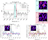 |
Fig. A.1. ID 7299, double-peak, GOLD category. Same as Fig. 3. A threshold of 50 (red dashed line in panel (a)) discards peak B while panel (e) shows a significant detection in the NB image (labelled 0) as well as an extracted spectrum in orange having the same shape as the reference spectrum. |
A.2. Threshold determination on NB images
In order to detect emission on NBs, a threshold of 2σ on three connected pixels has been chosen (Sect. 3.3). This choice has been made for two reasons. The first reason is to be coherent with the criterion used to detect areas of signal on the spectrum (Sect. 3.2): we used a minimum S/N of one per pixel for at least two adjacent pixels, which is similar to only one pixel with a S/N of 2. The second reason why we did not choose more strict parameters to avoid false detections, like the ones in Fig. 3 (detections labelled ’0’, ’2’ and ’3’), is to be able to detect compact and faint objects such as in the BRONZE category. Using a threshold of 2σ on the NB is thus a valid choice as we want to be consistent and inclusive.
We tested two different configurations on the parent sample: without the deblending function and with the default parameters of the deblending function6 of SourceFinder. While not using the deblending function, emission from other galaxies present on the NB image and close enough to our source is blended with the actual emission of our source. When looking at the same galaxies with the deblending function on, in this configuration, the different emissions are well differentiated. For this study, we choose to use the deblending function of photutils.SourceFinder, which will differentiate sources with a 7.5 magnitude difference (contrast = 0.001, default value).
Appendix B: SILVER category
Example of SILVER category with two detections in the reference segmentation map for each peak.
 |
Fig. B.1. ID 163, double-peak, SILVER category. Same as Fig. 3. We notice in panel (b) two clumps that are detected by SourceFinder in panel (d). The two clumps have the same spectral shape. |
Appendix C: Tables
First ten lines of the single-peaks table. The full table will be available online.
First ten lines of the double-peaks table. The full table will be available online.
First ten lines of the triple-peaks table. The full table will be available online.
Appendix D: Spectra
In this appendix we show the spectra of the whole parent sample categorised by their spectral classification: no-peak, single-peak, double-peak and triple-peak (see Sect. 4.1 and Table 3). The images are available at the following link: https://zenodo.org/records/14235906.
Appendix E: Evolution of the fraction of double-peaks for the GOLD and SILVER galaxies in the unbiased sample
As our sample is divided by spatial category (GOLD, SILVER and BRONZE) in addition to the spectral ones, it is interesting to see if the evolution of the fraction of double-peaks changes in function of the spatial category of the galaxies. In order to observe this evolution, we use the inclusive unbiased double-peak sample UDPI, which contains more double-peaks (i.e. more statistics) than the restrictive unbiased double-peak sample UDPR. It is important to note here that the inclusive unbiased double-peak sample UDPI only contains GOLD and SILVER galaxies. We refer the reader to Sect. 4.1.3 for more details.
To investigate if the fraction of double-peaks of the different categories varies with luminosity, we apply the same procedure as in Sect. 4.3.2. We divide our unbiased sample into four Lyα luminosity bins with the same number of objects. Left panel of Fig. E.1 shows the fraction of double-peaks for each of the four luminosity bins for U and for the GOLD and SILVER categories (in yellow and grey in the figure, respectively). The fraction of GOLD double-peaks evolves from around 34% for the faintest luminosities to 56% for the brightest bin (41.7 < log(LLyα [erg s−1]) < 43). On the other hand, there is no double-peaked SILVER objects at the faintest luminosities. Their fraction reaches almost 10% for intermediate Lyα luminosities (41.2 < log(LLyα [erg s−1]) < 41.7) before dropping to 4% the higher values, due to the significant lack of objects in our parent sample at such luminosities. SILVER double-peaks appear to not be faint objects but rather luminous ones. The fraction of GOLD double-peaks shows a similar trend as the fraction of the whole sample (black dots in left panel of Fig. E.1), mainly explained by the high number of GOLD galaxies populating the sample compared to the SILVER ones.
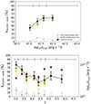 |
Fig. E.1. Fraction of double-peaked LAEs plotted against the logarithmic Lyα luminosity and the redshift. Left panel: Fraction of double-peaked LAEs plotted against the logarithmic Lyα luminosity. The unbiased sample U has been divided into four luminosity bins with the same number of objects (51 or 52). The fraction of double-peaks has been derived in each bin. The results are positioned at the median Lyα luminosity of each bin. The horizontal black line at the top of the figure shows the size of each Lyα luminosity bin. Right panel: Fraction of double-peaked LAEs plotted against the redshift. The unbiased sample U has been divided into eight redshift bins with the same number of objects (25 or 26). The fraction of double-peaks has been derived in each bin. The results are positioned at the median redshift of each bin. The black stars surrounded in red represent the mean Lyα luminosity of each bin. The black dots represents the total fraction of double-peaks (NUDPI/NU). The UDPI is composed of GOLD and SILVER double-peaks. The yellow dots show the fraction of GOLD double-peaks (NUDPI GOLD/NU) among U. The fraction of SILVER double-peaks (NUDPI SILVER/NU) is represented by the grey dots. |
We also repeat the same procedure to the evolution of the double-peak fraction with redshift. Right panel of Fig. E.1 shows the evolution of the fraction of double-peaks with redshift for U in black, the GOLD double-peaks in yellow (NUDPI GOLD/NU) and the SILVER double-peaks in grey (NUDPI SILVER/NU). At low redshift (z < 3.5), we see an interesting increase in the double-peak fraction driven by the SILVER sample. If this trend is confirmed with more data, it could indicate an intrinsic evolution of the LAE population towards cosmic noon, as SILVER objects are composed of multiple clumps of Lyα emission. If such a possible evolution is confirmed, it could make less pertinent the use of the double-peak fraction to probe the opacity of the IGM at this redshift regime. At redshift above 5, no more SILVER objects are observed, the double-peak fraction being entirely driven by the GOLD sample.
Appendix F: Objects with systemic redshift
From nebular lines also observed in MUSE spectra, 15 galaxies from the parent sample have a secure systemic redshift. We refer the reader to Sect. 5.3 for more details. The image is available at the following link: https://zenodo.org/records/14235906.
All Tables
Overview of the samples used in this paper and the number of sources contained in each of them.
Comparison of the classification results with different threshold values (N = 30, 40 and 50) before performing the NB image verification described in Sect. 3.2.
Comparison of the classification results with different threshold values (N = 30, 40 and 50) after performing the NB image verification described in Sect. 3.3.
First ten lines of the single-peaks table. The full table will be available online.
First ten lines of the double-peaks table. The full table will be available online.
First ten lines of the triple-peaks table. The full table will be available online.
All Figures
|
Fig. 1. Exposure time map of the MXDF. The blue circles are the MXDF-selected objects, the pink triangles indicate the UDF-10-selected targets and the green squares the MOSAIC-selected objects (see Sect. 2.2). The field is coloured by exposure time in hours, from 0 h to 140 h. The red contour represents the 100 h limit of the field. The solid and dashed white contours show the 30 h and 10 h exposure time of the MXDF, respectively. The UDF-10-selected objects present in the deepest part of the field have their Lyα line in the AO gap. |
| In the text | |
|
Fig. 2. Flowchart of the method. The input data are indicated by green boxes at the top of the figure. Black boxes refer to the different steps of the method. The corresponding sections of the paper are shown in blue. The orange boxes inside the black ones indicate the output data. The visual classification is shown by a triangle (see Sect. 3.4). The GOLD, SILVER, and BRONZE categories are illustrated by a gold, a grey, and a brown rectangle, respectively. The spectral shapes of the Lyα emission are indicated by circles, black for single- and triple-peaks and red for double-peaks. The box at the bottom presents the Lyα spectral parameters (black) and the spectral parameters measured for double-peak objects (red), detailed in Sect. 3.5. |
| In the text | |
|
Fig. 3. ID 3240, double-peak, GOLD category. (a): Example of a detection spectrum in black obtained from the 100 realizations of the original spectrum (Sect. 3.2). The S/N spectrum of the original spectrum is plotted in dotted black. The horizontal dashed green line shows our detection threshold of N = 40 defining areas of signal. The blue A and red B shaded areas correspond to the areas of signal obtained by the crossing of the detection spectrum with the threshold line of N = 40. (b) and (c): 50 × 50 kpc2 NB images of the area of signal A and the area of signal B, respectively. The black cross represents the centre coordinates of the source. The white contours correspond to a S/N level of 2. (d) and (e): Spectra extracted from the photutils.SourceFinder segmentation maps (Sect. 3.3). The colour of each spectrum matches the NB image segmentation map colour inserted in the plot. Only the blue spectrum extracted from the blue SourceFinder segmentation map number ‘1’ contributes to the Lyα line. The reference spectrum (Sect. 2.3) in black dashed line is displayed as a reference. The dashed contours on the NB images represent the reference segmentation maps used in B23. The grey dashed contour is the segmentation map of the targeted source, the green ones correspond to other objects. |
| In the text | |
|
Fig. 4. Illustrations of GOLD, SILVER and BRONZE double-peaked galaxies. Left panel: Illustration of a GOLD double-peaked galaxy. The emission of each peak (red circle) is located inside the segmentation map (black contour) at the same spatial location. Middle panel: SILVER category. Each peak of the double-peaked Lyα line is coming from two different locations inside the segmentation map. Right panel: Case of a BRONZE galaxy. The blue peak (A) is emitted in a certain region and the red peak (B) is emitted in a different region of the segmentation map. |
| In the text | |
|
Fig. 5. Examples of the different spectral shape categories (Sect. 4.1), except the ‘no-peak’ category (see Appendix D). First row: spectra of single-peak galaxies. Second and third rows: spectra from sources belonging to the double-peak category, red and blue dominated spectra, respectively. Last row: spectra showing triple-peak Lyα lines. We note that the y-axis shows the flux normalized to the maximum of each line. |
| In the text | |
|
Fig. 6. Cumulative fraction of double-peaks with increasing S/N. The vertical dash-dotted line represents the S/N cut used to prevent missing the detection of double-peaks at lower S/N as the fraction of double-peaks drops below this value. |
| In the text | |
|
Fig. 7. Figures illustrating the observational limitations of our sample. GOLD, SILVER, and BRONZE objects are represented by triangles, crosses, and squares symbols, respectively. Left: Lyα luminosity as a function of redshift for the parent sample. The horizontal black dash-dotted line represents the luminosity cut (LLyα = 3 × 1040 [erg s−1]) used to mitigate the redshift dependence. Middle: B/T flux ratio as a function of S/N (calculated as described in Sect. 3.5) for the whole double-peak sample. B/T ≈ 0 objects can be seen in Appendix D. They have a very small blue peak. The horizontal grey dashed line at B/T = 0.5 marks the blue-dominated versus red-dominated dividing line. The vertical black dash-dotted line represents the S/N cut (S/N = 7) made to balance the demands of being able to detect extreme B/T and keeping a representative subsample of double-peaks. The dashed lines mark boundaries of 1/(S/N) < B/T < 1–1/(S/N). Three objects have a B/T > 1 because the total flux is smaller than the flux in the blue peak because the continuum is negative between the peaks (see Appendix D). Right: Peak separation as a function of redshift for the whole double-peak sample. The horizontal black dash-dotted line represents the vsep cut (vsep = 150 km s−1) used to account for the spectral resolution of MUSE. For both the Lyα luminosity and the vsep, the observational sensitivity and spectral resolution curves are not straight lines. The ones shown in the plots are our selection limits. |
| In the text | |
|
Fig. 8. Physical parameter distributions of the unbiased samples. (a): Logarithmic Lyα luminosity distribution. (b): FWHM distribution of the peak of the Lyα line with the strongest flux. (c): B/T distribution measured on the Lyα emission lines of the double-peaked objects. B/T = 0.5 is represented by a black dash-dotted line. The numbers written in black and orange correspond to the number of galaxies having a B/T value below 0.5 (N = 57 for UDPI and N = 51 for UDPR) and above 0.5 (N = 48 for UDPI and N = 15 for UDPR). (d): Peak separation distribution of the double-peak samples. In orange are represented the restrictive samples: U ∖ {UDPR} in dashed lines and UDPR in solid line. In black are represented the inclusive samples: U ∖ {UDPI} in dotted lines and UDPI in solid line. |
| In the text | |
|
Fig. 9. Peak separation plotted against the redshift for our double-peak sample and for several studies (Kulas et al. 2012; Yamada et al. 2012; Hashimoto et al. 2015; Matthee et al. 2018; Songaila et al. 2018; Bosman et al. 2020; Meyer et al. 2021; Naidu et al. 2022). Our double-peak sample represented in purple shows three different symbols for the three categories GOLD (triangle), SILVER (cross), and BRONZE (square). A horizontal black dash-dotted line at 150 km s−1 represents the peak separation threshold made in Sect. 4.1.2 to obtain the fraction of double-peaks. The peak separations are in discrete lines due to the fact that the minimal peak separation measured is two spectral bins and depends on redshift. |
| In the text | |
|
Fig. 10. Fraction of double-peaked LAEs plotted against the logarithmic Lyα luminosity. The unbiased sample U has been divided into four luminosity bins with the same number of objects (51 or 52). The fraction of double-peaks has been derived in each bin for both UDPI and UDPR. The results are positioned at the median Lyα luminosity of each bin. The fractions of inclusive double-peaks are represented in black colour. The XDP R of the restrictive sample are in orange. The horizontal black line at the top of the figure shows the size of each Lyα luminosity bin. |
| In the text | |
|
Fig. 11. B/T flux ratio distributions shown for bright and faint galaxies. Top panel: B/T flux ratio distributions of the inclusive unbiased double-peak sample (UDPI) divided into two Lyα luminosity bins with the same number of objects (53 and 52). The faint subsample (LLyα < 3.7 × 1041 erg s−1) is in black and the bright one (LLyα > 3.7 × 1041 erg s−1) is in grey. Bottom panel: B/T flux ratio distributions of the restrictive unbiased double-peak sample (UDPR) divided into two Lyα luminosity bins with the same number of objects (33 and 33). The faint subsample (LLyα < 3.9 × 1041 erg s−1) is in stepped orange and the bright one (LLyα > 3.9 × 1041 erg s−1) is in orange. B/T = 0.5 is represented by a black dash-dotted line in both panels. |
| In the text | |
|
Fig. 12. Fractions of double-peaked LAEs plotted against the redshift. The unbiased sample has been divided into eight redshift bins with the same number of objects (25 or 26). The fraction of double-peaks has been derived in each bin. The results are positioned at the median redshift of each bin. The fractions of inclusive double-peaks are represented in black colour. The XDP of restrictive objects are in orange. The horizontal black line at the top of the figure shows the size of each redshift bin. The black stars surrounded in red represent the mean Lyα luminosity of each bin. |
| In the text | |
|
Fig. 13. ID 399, double-peak, BRONZE category. Example of a LAE surrounded by a satellite discovered thanks to our method. (a)–(c): Same as Fig. 3. The cyan circle b1 and the orange circle b2 represent the apertures used to extract two spectra at the indicated locations. The size of the circles represent a 0.5″ diameter aperture. (d): 50 × 50 kpc2 HST F125W image with the two locations of the extraction (cyan and orange circles). (e): Spectra extracted from the two circles. The orange dash-dotted line corresponds to the spectrum extracted at the position of b2. The spectrum extracted from b1 is shown as a cyan dashed line. The black line is the summed spectrum of the blue and orange spectra. The spectrum extracted at the position b2, that is the position of the satellite, contributes mainly to the peak B. |
| In the text | |
|
Fig. 14. ID 8439, double-peak, BRONZE category. Same as Fig. 3. Peaks A and B come from two different spatial locations. Peak A is the Lyα emission of the halo of ID 8455 (contained in the reference segmentation map of ID 8439). Peak B is the Lyα emission coming from the targeted galaxy. |
| In the text | |
|
Fig. 15. ID 7817, single-peak, GOLD category. Example of a pair of galaxies. The galaxy ID 8271 has the same redshift as ID 7817 (z ≈ 4.14). |
| In the text | |
|
Fig. 16. ID 412, double-peak, GOLD category. Same as Fig. 3. Example of a triplet system of galaxies (ID 412, 6698 and 8355) at z ≈ 4.13. Interestingly, in panel e, two galaxies have a similar red-dominated double-peaked Lyα line profile while the third one, labelled 1, shows a blue-dominated double-peak line. |
| In the text | |
|
Fig. 17. Velocities of every peak and trough for the double-peaked galaxies having a systemic redshift (Sect. 5.3). Each line corresponds to a source, where the blue (red) circle shows the bluer (redder) peak and the green square indicates the position of the trough. The larger circle represents the peak with the highest flux. The first line of the bottom part of the figure shows the mean positions of the trough and the blue and red peaks of the objects shown above (without taking into account ID 263). The mean LBG and mean Green Pea (GP) are drawn from the literature, Kulas et al. (2012) and Orlitová et al. (2018), respectively. |
| In the text | |
|
Fig. A.1. ID 7299, double-peak, GOLD category. Same as Fig. 3. A threshold of 50 (red dashed line in panel (a)) discards peak B while panel (e) shows a significant detection in the NB image (labelled 0) as well as an extracted spectrum in orange having the same shape as the reference spectrum. |
| In the text | |
|
Fig. B.1. ID 163, double-peak, SILVER category. Same as Fig. 3. We notice in panel (b) two clumps that are detected by SourceFinder in panel (d). The two clumps have the same spectral shape. |
| In the text | |
|
Fig. E.1. Fraction of double-peaked LAEs plotted against the logarithmic Lyα luminosity and the redshift. Left panel: Fraction of double-peaked LAEs plotted against the logarithmic Lyα luminosity. The unbiased sample U has been divided into four luminosity bins with the same number of objects (51 or 52). The fraction of double-peaks has been derived in each bin. The results are positioned at the median Lyα luminosity of each bin. The horizontal black line at the top of the figure shows the size of each Lyα luminosity bin. Right panel: Fraction of double-peaked LAEs plotted against the redshift. The unbiased sample U has been divided into eight redshift bins with the same number of objects (25 or 26). The fraction of double-peaks has been derived in each bin. The results are positioned at the median redshift of each bin. The black stars surrounded in red represent the mean Lyα luminosity of each bin. The black dots represents the total fraction of double-peaks (NUDPI/NU). The UDPI is composed of GOLD and SILVER double-peaks. The yellow dots show the fraction of GOLD double-peaks (NUDPI GOLD/NU) among U. The fraction of SILVER double-peaks (NUDPI SILVER/NU) is represented by the grey dots. |
| In the text | |
Current usage metrics show cumulative count of Article Views (full-text article views including HTML views, PDF and ePub downloads, according to the available data) and Abstracts Views on Vision4Press platform.
Data correspond to usage on the plateform after 2015. The current usage metrics is available 48-96 hours after online publication and is updated daily on week days.
Initial download of the metrics may take a while.