| Issue |
A&A
Volume 691, November 2024
|
|
|---|---|---|
| Article Number | A66 | |
| Number of page(s) | 9 | |
| Section | Extragalactic astronomy | |
| DOI | https://doi.org/10.1051/0004-6361/202347958 | |
| Published online | 29 October 2024 | |
Spatially resolved spectroscopic analysis of Lyα haloes
Radial evolution of the Lyα line profile out to 60 kpc
1
Univ Lyon, Univ Lyon1, Ens de Lyon, CNRS, Centre de Recherche Astrophysique de Lyon UMR5574, F-69230 Saint-Genis-Laval, France
2
Leibniz-Institut fur Astrophysik Potsdam (AIP), An der Sternwarte 16, 14482 Potsdam, Germany
3
Observatoire de Geneve, Universite de Geneve, 51 Ch. des Maillettes, 1290 Versoix, Switzerland
4
Leiden Observatory, Leiden University, P.O. Box 9513 2300 RA Leiden, The Netherlands
5
Department of Physics, ETH Zürich, Wolfgang-Pauli-Strasse 27, 8093 Zürich, Switzerland
6
Department of Astronomy, University of Texas at Austin, 2515 Speedway, Austin, TX 78712, USA
7
Max Planck Institute for Astronomy, Königstuhl 17, 69117 Heidelberg, Germany
8
Observatoire de Genève, Université de Genève, Ch. Pegasi 51, CH-1290 Versoix, Switzerland
9
Instituto de Astrofísica e Ciências do Espaço, Universidade do Porto, CAUP, Rua das Estrelas, PT4150-762 Porto, Portugal
10
Departamento de Física e Astronomia, Faculdade de Ciências, Universidade do Porto, Rua do Campo Alegre 687, PT4169-007 Porto, Portugal
11
National Astronomical Observatory of Japan (NAOJ), 2-21-1, Osawa, Mitaka, Tokyo 181-8588, Japan
⋆ Corresponding author; This email address is being protected from spambots. You need JavaScript enabled to view it.
Received:
13
September 2023
Accepted:
26
July 2024
Abstract
The extended Lyα haloes (LAHs) have been found to be prevalent around high-redshift star-forming galaxies. However, the origin of the LAHs is still a subject of debate. The spatially resolved analysis of Lyα profiles provides an important diagnostic. We analyse the average spatial extent and spectral variation of the circumgalactic LAHs by stacking a sample of 155 Lyα emitters (LAEs) at redshifts of 3 < z < 4 in the MUSE Extremely Deep Field. Our analysis reveals that, with respect to the Lyα line of the target LAE, the peak of the Lyα line at large distances becomes increasingly more blueshifted up to a projected distance of 60 kpc (≈3× virial radius), with a velocity offset of ≈250 km/s. This trend is evident in both the mean and median stacks, suggesting that it is a general property of our LAE sample, which typically has a Lyα luminosity of ≈1041.1 erg s−1. However, due to the absence of systemic redshift data, it remains unclear whether the Lyα line peak at large projected distances is less redshifted compared to the inner regions or truly blueshifted with respect to the systemic velocity. We explore various scenarios to explain the large-scale kinematics of the Lyα line.
Key words: galaxies: evolution / galaxies: formation / galaxies: high-redshift / intergalactic medium / cosmology: observations
© The Authors 2024
 Open Access article, published by EDP Sciences, under the terms of the Creative Commons Attribution License (https://creativecommons.org/licenses/by/4.0), which permits unrestricted use, distribution, and reproduction in any medium, provided the original work is properly cited.
This article is published in open access under the Subscribe to Open model. This email address is being protected from spambots. You need JavaScript enabled to view it. to support open access publication.
1. Introduction
The exchange of mass, momentum, and energy between a galaxy and the intergalactic medium (IGM) plays a crucial role in regulating galaxy evolution. The circumgalactic medium (CGM), which forms the transition region between the galaxy and the IGM, offers a detailed record of the relevant physical processes at play (e.g. Tumlinson et al. 2017). Throughout the epoch of galaxy evolution, the CGM is continuously enriched and depleted by galactic outflows, inflows, and mergers. Investigating the different components of the CGM and understanding their connection to the galaxy’s star formation activity and interstellar medium (ISM) are of critical importance for understanding galaxy evolution (e.g. Hopkins et al. 2018; Thompson & Heckman 2024).
The hydrogen Lyα line is a powerful tool for tracing the galaxies at high redshift and mapping their CGM and IGM. Large samples of star-forming galaxies at z ≳ 2 characterised by strong Lyα emission, known as Lyα emitters (LAEs), have been efficiently identified in deep narrow-band (NB) imaging (e.g. Gronwall et al. 2007; Ouchi et al. 2008; Shibuya et al. 2012; Kikuta et al. 2023) and spectroscopic observations (e.g. Rauch et al. 2008; Guo et al. 2020a; Richard et al. 2021). The spatially integrated Lyα emission line is almost always redshifted relative to the systemic velocity (e.g. Yamada et al. 2012; Chonis et al. 2013), which is thought to be due to the scattering of Lyα photons in a galactic outflow (e.g. Ahn et al. 2003; Erb et al. 2014; Shibuya et al. 2014). The Lyα emission extended at the circumgalactic scale, known as Lyα haloes (LAHs), is detected individually (e.g. Rauch et al. 2008; Wisotzki et al. 2016) and through stacking (e.g. Hayashino et al. 2004; Momose et al. 2014; Wisotzki et al. 2018). The integral field unit (IFU) facilities, such as the ESO-VLT instrument Multi Unit Spectroscopic Explorer (MUSE, Bacon et al. 2010) and the Keck Cosmic Web Imager (KCWI, Martin et al. 2010; Morrissey et al. 2012) have enhanced the efficiency of detecting LAHs around galaxies at 2 ≲ z ≲ 6. We now know that the star-forming galaxies are ubiquitously surrounded by LAHs that are observed to be several to tens of times larger than the stellar continuum, indicating the presence of a significant amount of neutral hydrogen in the circumgalactic gas (e.g. Steidel et al. 2011; Ouchi et al. 2020; Kusakabe et al. 2022). Recent deep observations and stacking analyses have detected extended Lyα emission around LAEs out to hundreds of kiloparsecs (kpc), achieving a surface brightness level of ≈10−20 erg s−1 cm−2 arcsec−2 (e.g. Kikuchihara et al. 2022; Lujan Niemeyer et al. 2022; Guo et al. 2024).
Despite the fact that most studies of LAHs focus on mapping the surface brightness of the extended Lyα emission, the spatially resolved spectral variation is still poorly constrained. Observing the spectral variation of the LAHs is of vital importance in understanding their physical nature, because it is related to physical properties of the CGM, such as geometry, gas column density, covering fraction, kinematics, and dust content (e.g. Verhamme et al. 2006; Dijkstra 2014; Chang et al. 2023). IFU observations of LAHs have so far only been performed on a few gravitationally lensed (Patrício et al. 2016; Claeyssens et al. 2019; Solimano et al. 2022) and unlensed (Erb et al. 2018, 2023; Leclercq et al. 2020) LAHs, which, restricted by S/N, can only be used to study the luminous outliers at small impact parameters (10–30 kpc). In terms of how the Lyα profile varies with distance, Claeyssens et al. (2019) and Leclercq et al. (2020) found a trend whereby the peak of the Lyα line is shifted to redder wavelengths at large distances (≈20 kpc) from the central galaxy, and that there is a strong correlation between this peak velocity shift and line width, which can be explained by models of Lyα resonant scattering in outflows. However, several other observations give contradictory results. For example, in a single case study of an LAE with a particular double-peaked Lyα profile, Erb et al. (2018) found higher blue-to-red peak ratios and narrower separations of the two peaks at larger radii (≲30 kpc). Erb et al. (2023) extended the study by analysing a sample of 12 double-peaked LAEs, and found similar trends in peak ratios and separations to Erb et al. (2018). Models have been used to reproduce the spatially resolved Lyα profiles (e.g. Zheng & Miralda-Escudé 2002; Song et al. 2020). From the simulation point of view, the variety of the Lyα line shapes depends not only on the complicated radiative transfer effect in the galaxy’s ISM and CGM, but also on the galaxy’s evolutionary phase and the positional angle looking at the galaxy (Blaizot et al. 2023).
Despite previous spectroscopic observations of bright LAHs, the characteristic pattern in the spatial variations of the Lyα line profile across the LAH population remains unclear. Elucidating this problem requires a large sample of LAEs in order to average out the variation between individual LAEs and deep observations to detect the very low-surface-brightness emission, which is difficult and expensive for current observing facilities. We thus have to rely on data stacking. The pioneering MUSE stacking analysis (Gallego et al. 2021) suggests that the peak of the Lyα emission is bluer at large radii, although with high noise in the spectra. More representative samples of LAEs are needed to investigate the faint LAE population. Higher S/N spectra are also needed to precisely understand the average Lyα line profile and its velocity shift.
In this work, we aim to obtain a comprehensive understanding of the average spectral variations of LAHs, particularly for the collective population of MUSE-detected LAEs, the majority of which have low Lyα luminosity and a single redshifted Lyα peak. We make use of the dataset of MUSE eXtremely Deep Field survey (MXDF, Bacon et al. 2023), which is the deepest spectroscopic datacube ever obtained. The MXDF is at least three to ten times deeper than the datasets used in Gallego et al. (2021), allowing the identification of a population of much fainter LAEs and the detection of diffuse Lyα emission at an unprecedentedly low surface-brightness limit. In our previous work (Guo et al. 2024, hereafter Paper I), we measured the median Lyα surface brightness profiles out to 270 kpc. In this paper, we focus on the evolution of the Lyα spectral profiles with distance. We adopt the standard ΛCDM cosmology with H0 = 70 km s−1 Mpc−1, Ωm = 0.3, and Ωλ = 0.7. All distances are proper, unless noted otherwise.
2. Data description and analysis
The MXDF (Bacon et al. 2023) has a field of view of 1′ in diameter, with the longest exposure time being approximately 140 hours, and the shortest exposure time being several hours, reaching an unresolved emission line median 1σ surface brightness limit of < 10−19 erg s−1 cm−2 arcsec−2. The very deep exposure of the MXDF enables studies of extremely low-surface-brightness emission, such as the detection of a cosmic web in Lyα emission on scales of several comoving megaparsecs (cMpc) shown in Bacon et al. (2021). The survey design, sky coverage, and data reduction of the MXDF are described in Bacon et al. (2023). These authors also provide redshifts, multi-band photometry, morphological and spectral properties, and measurements of the stellar mass and star formation rate of all the galaxies discovered by the deep MUSE observations in the Hubble ultradeep field (HUDF).
A total of 420 LAEs have been detected in the MXDF at 3 ≲ z ≲ 6.5. In this study, we focus on LAEs in the redshift range of 3 < z < 4, where the cosmological surface brightness dimming is relatively weak, the IGM absorption is low, the efficiency of MUSE is high, and there is no strong atmospheric OH emission. There are 155 LAEs in this redshift range. The distribution of redshift, Lyα luminosity, Lyα line rest-frame FWHM, and S/N of Lyα line of the LAE sample can be found in Fig. 1 of Paper I. The median redshift is 3.41. The median Lyα luminosity (LLyα) of these LAEs is approximately 1041.1 erg s−1, with a 90th percentile of 1041.8 erg s−1 and a 10th percentile of 1040.6 erg s−1. The median stellar mass (M*) is approximately 107.6 M⊙. These characteristics make our sample representative of the fainter and lower mass populations of LAEs compared to previous studies (e.g. Leclercq et al. 2020; Gallego et al. 2021; Erb et al. 2023). More details of this LAE sample are presented in Bacon et al. (2023) and Paper I. In Paper I, we estimate the typical virial radius (rvir) of this LAE sample based on the rvir – UV magnitude relation predicted by the semi-analytic model of Garel et al. (2015). The typical virial radius rvir of the sample is approximately 20 kpc. The median M* of the LAE sample also corresponds to a similar estimation of rvir ≈ 23 kpc based on the stellar-to-halo mass relation given in Girelli et al. (2020). In the wavelength range corresponding to 3 < z < 4, the spectral resolution of MUSE is approximately 150 km/s.
We produce a 21″ × 21″ MUSE mini-datacube centred on each LAE. We mask all areas with an exposure time of less than 110 hours to achieve a high S/N. We remove the continuum by performing spectral median filtering using a wide spectral window of 200 Å. This approach provides a fast and efficient way to remove continuum sources in the search for extended line emission, as presented in previous studies (e.g. Wisotzki et al. 2016; Guo et al. 2020b; Borisova et al. 2016). We note that the major conclusions of this paper do not change if we change the spectral window of median filtering from 100 Å to 300 Å. We also mask all the emission and absorption lines from neighbouring objects based on the line catalogue and segmentation maps provided by Bacon et al. (2023).
To study the average spatially resolved spectra of the LAHs, we adopt a full 3D stacking procedure. We shift individual mini-datacubes and rebin them to a common (rest-frame) wavelength frame based on the peak wavelength of the Lyα line. For LAEs with double-peaked Lyα lines, we use the wavelength of the red peak. We produce stacked datacubes using both mean and median stacking.
3. Results
3.1. The large-scale kinematics of Lyα line
In Figure 1 we present the Lyα pseudo-NBs in a series of velocity bins of 200 km/s, with the full velocity coverage from –700 km/s to 700 km/s. These Lyα maps are extracted from the median-stacked datacube. The width of the pseudo-NBs (200 km/s) corresponds to approximately 0.8 Å at rest frame, and about 2–4 wavelength layers in the original MUSE datacubes. The middle velocity bin is centred on the Lyα line peak of the central galaxy. To improve the visualization of large-scale features, we spatially smoothed the NBs with a Gaussian filter with a FWHM of 2.3″.
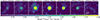 |
Fig. 1. Surface brightness maps of the median-stacked Lyα emission. Each panel shows the Lyα pseudo-NB in a velocity interval of 200 km/s. The zero velocity corresponds to the peak of the Lyα line. The NBs have been smoothed using a Gaussian kernel of width of 2.3″. The grey contours correspond to Lyα significance levels of 2, 4, and 6σ (dotted, dashed, and solid, respectively). |
In Figure 1 we clearly see that the Lyα emission extends to several tens of kpc. The most extended Lyα emission does not reside at the peak of the Lyα line, but in the velocity range of [–300 km/s, –100 km/s], suggesting that the extended Lyα emission at large radii becomes bluer relative to the peak of the central Lyα line.
To confirm this blueshift trend of the extended Lyα emission (with respect to the Lyα red peak of the central galaxy), we measured the azimuthally averaged profiles of the Lyα line. The stacked spectra are shown in Figure 2. Different rows show different radial distances. In both mean (left) and median (right), the Lyα line shifts from approximately 0 km/s in the centre to approximately –250 km/s at ≈60 kpc. We note that the typical virial radius of the LAE sample is about 20 kpc, and so we are observing the large-scale Lyα kinematics out to approximately 3 rvir.
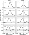 |
Fig. 2. Lyα line profiles at different distances from the central galaxy. The spectra in the left and right columns are derived from the mean- and median-stacked datacubes. Different rows show different radial bins ranging from 1″ (7 kpc) to 8″ (59 kpc). The vertical dashed lines denote the peak of the central Lyα line. The horizontal grey shaded regions show the 1σ error range. |
This blueshift trend of the Lyα line (with respect to the Lyα peak of the central galaxy) naturally produces different behaviours of the Lyα surface brightness profiles on the red and blue sides of the Lyα line peak. As is presented in Figure A.1, at large distances (tens of kpc), the bulk of the Lyα emission is bluer than the Lyα peak of the central galaxy, producing a flattening trend in the Lyα surface brightness profile. This flattening trend would be easily erased if the width of the pseudo-NB were too small. In Paper I, we measured the Lyα surface brightness profile using reasonably wide pseudo NBs (with a width of 920 km/s at z = 3), thus including most of the extended Lyα emission.
3.2. Error estimation
In Figure 2, we derive the noise of the spectra using the velocity range of ±1000–1500 km/s. In the largest radial bin (29–59 kpc), the peak S/N of the Lyα line is ≈3.2, and the accumulated S/N is ≈7.2. For the spectrum in each radial bin, we reproduced 200 mock spectra based on the noise distribution. We used these mock spectra to estimate the error of the Lyα peak velocity. The values are shown in each panel of Figure 2.
When we discuss the velocity shift, we must take into account the spectral resolution of MUSE, which is approximately 150 km/s in the wavelength range corresponding to 3 < z < 4, which is smaller than the measured Lyα line shift. While the low spectral resolution may limit the measurement accuracy of the peak velocity, it cannot produce the smooth trend of Lyα peak shift we see from 0 kpc to 60 kpc. To further eliminate its influence, in Appendix B we perform the stacking for LAEs at 4 < z < 5 following the same procedures as in Section 2. In this wavelength range, the spectral resolution of MUSE is slightly higher (approximately 110 km/s; see Fig. 15 of Bacon et al. 2017). We see very similar trends as in Figure B.1, but with lower S/N.
Another source of uncertainty comes from the measurement of the Lyα peak wavelength of the central galaxy. Bacon et al. (2023) provides the measurement errors for the Lyα peak wavelength. The median value of this error over the LAE sample is approximately 165.1 km/s. When considering the average over 155 LAEs, the stacked error should be approximately 14 km/s, which is evidently smaller than the velocity shift observed for the largest radial bin.
We also ensured that the stacking is not dominated by a few outliers, performing the following analysis. We randomly removed 15% of objects in the sample, and repeated the data stacking procedure. This process was iterated 100 times, and for each stack, we measured the Lyα peak velocity at 29–59 kpc. The resulting median velocity and its standard error are approximately –259 km/s and 18 km/s, respectively.
In summary, we detect a ≈250 km/s blueshift of the Lyα line (compared to the Lyα red peak of the central galaxy) from the galaxy out to 60 kpc (3 rvir). This blueshift trend is clearly observed in both mean and median stacks, and is not dominated by a few outliers. Hence, it is a common phenomenon for the population of LAEs.
3.3. Where is the systemic velocity?
In our previous analysis, we used the Lyα peak redshift (zLyα) of the target LAE as a reference for spectral realignment and data stacking. Due to the resonant nature of Lyα photons, the Lyα line usually deviates from the systemic redshift (zsys; e.g. McLinden et al. 2011; Erb et al. 2014; Shibuya et al. 2014; Muzahid et al. 2020). It is crucial to understand how the Lyα line profile evolves radially with respect to the systemic velocity. However, in our sample, we lack direct measurements of zsys.
We used the estimated zsys provided by Bacon et al. (2023). This estimate is based on the empirical relation established by Verhamme et al. (2018), which uses the Lyα peak separation (if two peaks of the Lyα line are detected) or the FWHM of the Lyα line (if only one peak is detected) to estimate the velocity offset between zLyα and zsys. We then realigned the mini-datacubes to the systemic velocity, and repeated the mean and median data stacking. The Lyα spectra in different radial bins are shown in Figure 3. In the inner ≈10 kpc, Lyα is redshifted by about 170 km/s relative to zsys. With increasing distance, the Lyα line shifts to shorter wavelengths. For the final radial bin (29–59 kpc), the peak of the Lyα line is slightly bluer than zsys, with a value of ≈–70 km/s. This trend can be seen in both the mean and median stacks.
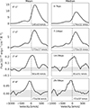 |
Fig. 3. As Figure 2, except that here all the mini-datacubes are realigned by the estimated zsys instead of zLyα. |
The scatter of the zsys estimate of Verhamme et al. (2018) is about 72 km/s. For a stack of 155 LAEs, the final error attributed to the zsys estimate should be only a few km/s. However, due to the noise level and the resolution of the spectra, the Lyα peak velocity in the final radial bin has a large uncertainty. We cannot confirm whether or not the Lyα peak at large distances (29–59 kpc) is more blueshifted than the systemic velocity.
4. Discussion
4.1. Average spectral morphology of the LAHs
Characterising the spatially resolved spectroscopic features of the LAHs is important for understanding the physical nature of these systems. Due to the faintness of the emission, previous work has mainly focused on a few bright or unique systems (e.g. Claeyssens et al. 2019; Leclercq et al. 2020; Erb et al. 2018, 2023). These latter authors found that the spectral morphology of the extended Lyα emission varies significantly between different LAHs, and even between different regions of an extended halo. However, a statistically robust general trend across the LAH population is still largely unknown.
In this study, we stacked a sample of LAEs at 3 < z < 4 observed by MUSE to study the typical spatial and spectral properties of the LAHs. We detect extended Lyα emission out to the largest radius of ≈60 kpc (approximately 3 rvir), and find an increasing blueshift trend of the Lyα line with respect to the central Lyα peak (Figures 2 and 3).
In Figure 4, we plot the Lyα peak velocity (with respect to the central Lyα peak) as a function of radial distance. The open circles and squares with error bars represent the mean and median stacks in Figure 2. The small symbols connected by dotted lines show the same trend, but with smaller radial bins. Although such a gradual trend of the Lyα line shifting blueward with increasing radius is robust, we cannot confirm whether the Lyα line at the largest radius (29–59 kpc) is truly bluer than the zsys because of the noise and the spectral resolution in the spectra, as discussed in Section 3.3.
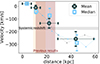 |
Fig. 4. Radial evolution of the Lyα peak velocity with respect to the Lyα line of the central LAE. The open circles and squares show the Lyα peak velocity shift in the mean and median stacks (Figure 2). The small symbols connected by dotted lines show the same results extracted with smaller radial bins. The grey horizontal shadow shows the median systemic redshift of the central LAE, as is shown in Figure 3, based on the empirical relations established by Verhamme et al. (2018). The orange and maroon vertical shadows show the maximum radii of the LAHs from previous MUSE (Leclercq et al. 2020; Claeyssens et al. 2019) and KCWI (Erb et al. 2018, 2023) analysis. |
In Figure 4, we also plot the maximum detection radii of the LAHs from the literature (Erb et al. 2018, 2023; Claeyssens et al. 2019; Leclercq et al. 2020). Before comparing our results with the literature, we note that we detect Lyα line profiles at much larger scales, not only in physical distance, but also with respect to the rvir of the system. The LAEs in these latter studies have much larger rvir than our LAE sample, because they are based on more luminous or more massive systems. For example, the LAE sample of Leclercq et al. (2020) has a median UV magnitude of approximately –19.2 mag, which, based on the rvir–UV magnitude relation given in Leclercq et al. (2017) and Garel et al. (2015), corresponds to rvir ≈ 50 kpc. The LAE sample of Erb et al. (2018, 2023) has a median stellar mass of 109.13 M⊙, corresponding to rvir ≈ 70 kpc based on the stellar-to-halo mass relation given in Girelli et al. (2020). Although this estimate of rvir is subject to large uncertainties, it does provide an indication of the different physical scales we are discussing: The maximum detection radii of the LAHs in Leclercq et al. (2020) and Erb et al. (2023) are approximately 19 kpc and 27 kpc, respectively, which means that they observe the Lyα lines within 50% of the rvir, namely the inner CGM. Our stack, however, reaches a much larger scale with respect to the typical virial radius of the system (60 kpc, or approximately 3 rvir), and thus we are analysing the physical processes that occur far beyond the inner CGM.
This large-scale velocity shift of the Lyα line shown in Figure 4 does not agree well with several previous analyses of individual LAHs, such as those of Claeyssens et al. (2019) and Leclercq et al. (2020). These authors find a trend that the Lyα line in the halo is redder compared to the Lyα line in the centre, although the trend has a large scatter. Limited by the S/N, the maximum radii of the LAHs in Claeyssens et al. (2019) and Leclercq et al. (2020) are about 9–19 kpc. As shown in Figure 4, the average Lyα peak shift within this radius is not obvious. This weak signal is difficult to distinguish because of the poor S/N and the intrinsic variation of the small sample.
The KCWI observations of Erb et al. (2018, 2023) on 13 double-peaked LAEs at z ∼ 2.3 reveal a similar trend to our work, in that the Lyα line becomes more blue-dominated with increasing radius, up to a maximum distance of ≈18–26 kpc. An advantage of Erb et al. (2018, 2023) is that they have a secure measurement of zsys from rest-frame optical emission lines, and so they find that the blue component (with respect to the systemic velocity) becomes more prominent at larger radii. The LAEs in Erb et al. (2018, 2023) are specifically selected to have low metallicity and high ionisation by extreme nebular emission line ratios, or to have very strong Lyα emission. It is therefore unclear whether we can generalise their conclusions to the LAE population. There are clear differences between our LAE sample and the LAEs in Erb et al. (2018, 2023). Their LAEs have a 2 dex higher median LLyα and a 1.5 dex higher median stellar mass than our sample. These differences in turn imply that at they are probing the inner CGM (≲0.5 rvir), while we are probing the very extended CGM out to approximately 3 rvir. This is likely the main origin of the difference between our results.
All the LAEs in Erb et al. (2018, 2023) have double peaked Lyα lines. Within the distance range of 11–26 kpc, the LAHs in Erb et al. (2018, 2023) always have two individual Lyα peaks on either side of the systemic velocity, while the relative strength of the two peaks changes with distance. Similarly, at the distance of ≲0.5 rvir, our stack finds a broad Lyα component bluer than the systemic velocity (top two rows of Figure 3), which results from the stacking of many blue Lyα lines at different velocities. However, at distances of greater than 14 kpc, we observe only a single Lyα peak. This single peak cannot solely be attributed to the lower spectral resolution of MUSE: The peak separation of Erb et al. (2018, 2023) at their largest radial bin ranges from approximately 300–800 km/s. If the MXDF LAEs have a similar peak separation to Erb et al. (2018, 2023), the two peaks could be resolved by MUSE.
The IGM absorption could remove the flux bluer than the systemic velocity, leading to underestimation of the Lyα blue peak flux. This systematic suppression of the Lyα blue peak with increasing redshift has been well analysed in previous work (e.g. Hayes et al. 2021). At the median redshift of z ∼ 3.4 of our LAE sample, the typical IGM transmission of Lyα is ≈60% (Laursen et al. 2011; Inoue et al. 2014). The poorly constrained zsys complicates our analysis: At large distances (29–59 kpc in Figure 3), if the Lyα line were still redder than the systemic velocity, the Lyα flux would not be strongly affected by the IGM transfer. However, if the opposite were true, the part of the Lyα flux that is bluer than the systemic velocity would be suppressed by IGM absorption by an average factor of 0.6.
4.2. Physical nature of the LAHs
Several physical mechanisms have been proposed to explain the production and propagation of Lyα photons in LAHs. Their relative importance may vary with radial distance (e.g. Mitchell et al. 2021; Byrohl et al. 2021). Here we explore several speculative considerations regarding the underlying physics responsible for the observed spectral shift of the Lyα line out to a distance of 60 kpc (approximately 3 rvir). Notably, a successful physical model should also account for the observed Lyα surface brightness profile, which shows a power-law decrease within 20 kpc and a tentative flat trend at 30–50 kpc (paper I).
The strongest peak of the Lyα line in most LAEs is observed to be redshifted relative to the systemic velocity (e.g. Yamada et al. 2012; Erb et al. 2014), which is commonly attributed to the complicated radiative transfer in outflows (e.g. Verhamme et al. 2006; Dijkstra & Kramer 2012; Blaizot et al. 2023). Models of Lyα photons scattering from a central source into an outflowing medium have successfully reproduced a large number of spatially integrated Lyα spectra (e.g. Hashimoto et al. 2015; Gronke 2017; Chang et al. 2023). Several previous works have attempted to explain the spatially resolved features of LAHs (e.g. Zheng & Miralda-Escudé 2002; Song et al. 2020). To account for the observed large-scale blueshift trend of the Lyα line with respect to the central LAE, one possibility is a gradually decelerating outflow, which is expected because of the increasing importance of gravitational deceleration towards larger radii. The decelerating outflow is expected to produce a Lyα line with a less-redshifted velocity offset with respect to the systemic velocity (e.g. Song et al. 2020; Garel et al., in prep.), but is unlikely to be able to produce a Lyα line bluer than systemic velocity. Radiative transfer modelling of Erb et al. (2023) finds a gradual deceleration or constant-velocity phase of the outflow at large radii, which can recover the increase in Lyα blue peak flux with distance. The LAEs of Erb et al. (2023) are double-peaked; most of their Lyα blue peaks at large radii are fainter than the red ones.
The simulations of Blaizot et al. (2023) suggest an alternative scenario where the strongest resonant scattering effects (broadening and redshifting of the line) occur in the inner CGM, where gas densities are high. Instead, the more extended CGM (between 0.2 and 3 rvir) is often dominated in volume by a hot and highly ionised outflow, which acts as a screen that intercepts blue Lyα photons from the galaxy and re-emits them approximately isotropically. This process is expected to produce a profile that increasingly moves blueward towards larger distances with respect to the central Lyα line.
Another scenario considers the role of inflows. Chung et al. (2019) simulate an LAH around a galaxy with a stellar mass of 1010.5 M⊙ (rvir ≈ 95 kpc based on Girelli et al. 2020) and suggest that galactic outflows primarily affect the Lyα properties within ≈50 kpc, while cold accretion flows dominate at larger radii. Based on the observation of an enormous Lyα blob, Li et al. (2022) provide a model in which the Lyα photons are produced by star formation in the galaxy and propagate outwards within multi-phase clumpy outflows. Near the blob outskirts, infalling cool gas shapes the observed blue-dominated Lyα line, albeit with a very small contribution to the total Lyα luminosity. This combination of outflows and inflows is also inferred from the H I absorption by Chen et al. (2020). These latter authors observe an asymmetry in the Lyα absorption line and explain it as infilling by blueshifted Lyα emission relative to zsys. They also claim a transition between outflow-dominated (r ≲ 50 kpc) and accretion-dominated flows (r ≳ 100 kpc) for galaxies with z ≈ 2.2 and M* ≈ 1010 M⊙ by comparing their observations with models. If we assume that the Lyα line at large distances (Figure 3) is indeed blueshifted with respect to the systemic velocity, then a scenario of large-scale gas inflows becomes reasonable, in which a non-negligible fraction of Lyα photons is propagated in gas inflows, and the gradual transition of the Lyα line from redshift to blueshift out to tens of kpc indicates a transition in the dominance of gas outflows to inflows.
From the perspective of the Lyα flux budget, scattering models in which all Lyα photons are scattered from a central source inherently predict a monotonically decreasing Lyα surface brightness profile, while our observations (Appendix A and Paper I) find a flattening trend at large distances. Paper I suggests that this trend requires additional sources of Lyα photons instead of scattering from the central galaxy; for example, in situ production of Lyα photons at large distances. The power source could be cooling radiation that converts gravitational energy into kinetic and thermal energy through collision (e.g. Haiman et al. 2000; Dijkstra et al. 2006; Rosdahl & Blaizot 2012). Fluorescence from the nearby galaxies or from the UV background can also produce Lyα photons at large radii (e.g. Gould & Weinberg 1996; Cantalupo et al. 2005; Mas-Ribas & Dijkstra 2016). If the in situ-produced Lyα photons are emitted from a static medium and escape directly without scattering, the Lyα line should be at exactly the systemic velocity. However, if the bulk of the locally produced Lyα photons are scattered in the CGM, the kinematics of the CGM gas would strongly influence the Lyα line profiles, with the gas inflows and outflows producing blue- and red-skewed Lyα profiles with respect to the systemic velocity.
Neighbouring galaxies could also contribute to the observed properties of LAHs, whether they are unresolved satellite galaxies (e.g. Momose et al. 2016; Mas-Ribas et al. 2017; Mitchell et al. 2021) or more massive nearby systems (e.g. Byrohl et al. 2021). Considering that the Lyα emission from the neighbouring galaxies is also regulated by similar mechanism(s) to the target galaxy, the Lyα emission escaping from these galaxies should also be redshifted on average relative to the systemic velocity. Assuming either radial infalling or virialised motions of the satellite galaxies, it is difficult to find a physical model that would systematically produce a radial blueshift (or less-redshift) trend in the stack. However, under the assumption that the unresolved satellites have lower star-formation rates and possibly drive weaker winds, we could expect smaller Lyα velocity offsets from satellite galaxies (Muzahid et al. 2020).
Overall, our observed Lyα peak shift appears to be a generic property of LAHs according to the MXDF data. A possible scenario would be that the Lyα line emerging at small projected radii results from the propagation of centrally emitted photons in outflowing gas, whereas the signal at the outskirts is more likely due to radiative transfer effects in infalling gas or decelerating outflows. Distinguishing between the two kinematic patterns requires a more robust measurement of zsys, which is not available at the time of this work. The Lyα photons in the outskirts are likely to be produced in situ by collision, fluorescent emission, or satellites. To investigate the physical nature of the LAHs, a better understanding of both the flux budget and the kinematic behaviour of the LAHs is required.
5. Summary
The main focus of this paper is to report a large-scale blueshift of diffuse Lyα emission (with respect to the Lyα line of the central LAE). This paper is based on a statistical analysis of a representative galaxy sample with a typical Lyα luminosity of 1041.1 erg s−1. Our results represent a common phenomenon across the LAE population down to its faint end. Thanks to the extremely deep MXDF survey and data stacking, we are able to detect the Lyα line profile out to 60 kpc (approximately 3 rvir), which is much further than any previous analyses based on a few bright LAEs (e.g. Leclercq et al. 2020; Erb et al. 2023). Our main results can be summarised as follows:
From the galaxy out to ≈60 kpc, we detect a ≈250 km/s blueshift of the Lyα emission line with respect to the Lyα peak of the target LAE. However, we cannot determine the relative velocity offset between the Lyα line at the large distance and the systemic velocity, and so we are unable to tell whether it is bluer or redder than zsys. We demonstrate that the stacking of the LAE sample is not dominated by outliers. The blueshift trend with respect to the central Lyα red peak is thus ubiquitous among LAEs at 3 < z < 4 with a median Lyα luminosity of LLyα = 1041.1 erg s−1.
We discuss the mechanisms that might explain the blueshift of the Lyα emission. Our observations favour a scenario in which the inner part of the LAH is dominated by resonant-scattered Lyα photons from the outflowing gas, while at large distances the outflows become gradually decelerated or inflows start to emerge out to ≈60 kpc. However, at large distances, we cannot rule out the contribution from other scenarios, such as fluorescent emission or satellites.
This work is clearly limited by the absence of zsys. The key to tackling this problem is to obtain the rest-frame optical spectra. Spatially and spectrally resolved analytical models and simulations would also allow a more informed interpretation of the observational data.
Acknowledgments
Y.G., R.B. and L.W. acknowledge support from the ANR/DFG grant L-INTENSE (ANR-20-CE92-0015, DFG Wi 1369/31-1). L.W. acknowledges support by the ERC Advanced Grant SPECMAG-CGM (GA101020943). J.Brinchmann acknowledges support by Fundação para a Ciência e a Tecnologia (FCT) through the research grants UID/FIS/04434/2019, UIDB/04434/2020, UIDP/04434/2020 and PTDC/FIS-AST/4862/2020. J.Brinchmann acknowledges support from FCT work contract 2020.03379.CEECIND.
References
- Ahn, S.-H., Lee, H.-W., & Lee, H. M. 2003, MNRAS, 340, 863 [Google Scholar]
- Bacon, R., Accardo, M., Adjali, L., Anwand, H., & Bauer, S. 2010, SPIE Conf. Ser., 7735, 773508 [NASA ADS] [Google Scholar]
- Bacon, R., Conseil, S., Mary, D., et al. 2017, A&A, 608, A1 [NASA ADS] [CrossRef] [EDP Sciences] [Google Scholar]
- Bacon, R., Mary, D., Garel, T., et al. 2021, A&A, 647, A107 [NASA ADS] [CrossRef] [EDP Sciences] [Google Scholar]
- Bacon, R., Brinchmann, J., Conseil, S., et al. 2023, A&A, 670, A4 [NASA ADS] [CrossRef] [EDP Sciences] [Google Scholar]
- Blaizot, J., Garel, T., Verhamme, A., et al. 2023, MNRAS, 523, 3749 [NASA ADS] [CrossRef] [Google Scholar]
- Borisova, E., Cantalupo, S., Lilly, S. J., et al. 2016, ApJ, 831, 39 [Google Scholar]
- Byrohl, C., Nelson, D., Behrens, C., et al. 2021, MNRAS, 506, 5129 [NASA ADS] [CrossRef] [Google Scholar]
- Cantalupo, S., Porciani, C., Lilly, S. J., & Miniati, F. 2005, ApJ, 628, 61 [Google Scholar]
- Chang, S.-J., Yang, Y., Seon, K.-I., Zabludoff, A., & Lee, H.-W. 2023, ApJ, 945, 100 [NASA ADS] [CrossRef] [Google Scholar]
- Chen, Y., Steidel, C. C., Hummels, C. B., et al. 2020, MNRAS, 499, 1721 [NASA ADS] [CrossRef] [Google Scholar]
- Chonis, T. S., Blanc, G. A., Hill, G. J., et al. 2013, ApJ, 775, 99 [NASA ADS] [CrossRef] [Google Scholar]
- Chung, A. S., Dijkstra, M., Ciardi, B., Kakiichi, K., & Naab, T. 2019, MNRAS, 484, 2420 [NASA ADS] [CrossRef] [Google Scholar]
- Claeyssens, A., Richard, J., Blaizot, J., et al. 2019, MNRAS, 489, 5022 [Google Scholar]
- Dijkstra, M. 2014, PASA, 31, e040 [Google Scholar]
- Dijkstra, M., & Kramer, R. 2012, MNRAS, 424, 1672 [NASA ADS] [CrossRef] [Google Scholar]
- Dijkstra, M., Haiman, Z., & Spaans, M. 2006, ApJ, 649, 14 [NASA ADS] [CrossRef] [Google Scholar]
- Erb, D. K., Steidel, C. C., Trainor, R. F., et al. 2014, ApJ, 795, 33 [Google Scholar]
- Erb, D. K., Steidel, C. C., & Chen, Y. 2018, ApJ, 862, L10 [Google Scholar]
- Erb, D. K., Li, Z., Steidel, C. C., et al. 2023, ApJ, 953, 118 [NASA ADS] [CrossRef] [Google Scholar]
- Gallego, S. G., Cantalupo, S., Sarpas, S., et al. 2021, MNRAS, 504, 16 [NASA ADS] [CrossRef] [Google Scholar]
- Garel, T., Blaizot, J., Guiderdoni, B., et al. 2015, MNRAS, 450, 1279 [Google Scholar]
- Girelli, G., Pozzetti, L., Bolzonella, M., et al. 2020, A&A, 634, A135 [NASA ADS] [CrossRef] [EDP Sciences] [Google Scholar]
- Gould, A., & Weinberg, D. H. 1996, ApJ, 468, 462 [Google Scholar]
- Gronke, M. 2017, A&A, 608, A139 [NASA ADS] [CrossRef] [EDP Sciences] [Google Scholar]
- Gronwall, C., Ciardullo, R., Hickey, T., et al. 2007, ApJ, 667, 79 [NASA ADS] [CrossRef] [Google Scholar]
- Guo, Y., Jiang, L., Egami, E., et al. 2020a, ApJ, 902, 137 [CrossRef] [Google Scholar]
- Guo, Y., Maiolino, R., Jiang, L., et al. 2020b, ApJ, 898, 26 [Google Scholar]
- Guo, Y., Bacon, R., Wisotzki, L., et al. 2024, A&A, 688, A37 [NASA ADS] [CrossRef] [EDP Sciences] [Google Scholar]
- Haiman, Z., Spaans, M., & Quataert, E. 2000, ApJ, 537, L5 [Google Scholar]
- Hashimoto, T., Verhamme, A., Ouchi, M., et al. 2015, ApJ, 812, 157 [Google Scholar]
- Hayashino, T., Matsuda, Y., Tamura, H., et al. 2004, AJ, 128, 2073 [Google Scholar]
- Hayes, M. J., Runnholm, A., Gronke, M., & Scarlata, C. 2021, ApJ, 908, 36 [Google Scholar]
- Hopkins, P. F., Wetzel, A., Kereš, D., et al. 2018, MNRAS, 480, 800 [NASA ADS] [CrossRef] [Google Scholar]
- Inoue, A. K., Shimizu, I., Iwata, I., & Tanaka, M. 2014, MNRAS, 442, 1805 [NASA ADS] [CrossRef] [Google Scholar]
- Kikuchihara, S., Harikane, Y., Ouchi, M., et al. 2022, ApJ, 931, 97 [NASA ADS] [CrossRef] [Google Scholar]
- Kikuta, S., Ouchi, M., Shibuya, T., et al. 2023, ApJS, 268, 24 [NASA ADS] [CrossRef] [Google Scholar]
- Kusakabe, H., Verhamme, A., Blaizot, J., et al. 2022, A&A, 660, A44 [NASA ADS] [CrossRef] [EDP Sciences] [Google Scholar]
- Laursen, P., Sommer-Larsen, J., & Razoumov, A. O. 2011, ApJ, 728, 52 [Google Scholar]
- Leclercq, F., Bacon, R., Wisotzki, L., et al. 2017, A&A, 608, A8 [NASA ADS] [CrossRef] [EDP Sciences] [Google Scholar]
- Leclercq, F., Bacon, R., Verhamme, A., et al. 2020, A&A, 635, A82 [NASA ADS] [CrossRef] [EDP Sciences] [Google Scholar]
- Li, Z., Steidel, C. C., Gronke, M., Chen, Y., & Matsuda, Y. 2022, MNRAS, 513, 3414 [NASA ADS] [CrossRef] [Google Scholar]
- Lujan Niemeyer, M., Komatsu, E., Byrohl, C., et al. 2022, ApJ, 929, 90 [NASA ADS] [CrossRef] [Google Scholar]
- Martin, C., Moore, A., Morrissey, P., et al. 2010, SPIE Conf. Ser., 7735, 77350M [Google Scholar]
- Mas-Ribas, L., & Dijkstra, M. 2016, ApJ, 822, 84 [Google Scholar]
- Mas-Ribas, L., Dijkstra, M., Hennawi, J. F., et al. 2017, ApJ, 841, 19 [Google Scholar]
- McLinden, E. M., Finkelstein, S. L., Rhoads, J. E., et al. 2011, ApJ, 730, 136 [Google Scholar]
- Mitchell, P. D., Blaizot, J., Cadiou, C., et al. 2021, MNRAS, 501, 5757 [Google Scholar]
- Momose, R., Ouchi, M., Nakajima, K., et al. 2014, MNRAS, 442, 110 [NASA ADS] [CrossRef] [Google Scholar]
- Momose, R., Ouchi, M., Nakajima, K., et al. 2016, MNRAS, 457, 2318 [NASA ADS] [CrossRef] [Google Scholar]
- Morrissey, P., Matuszewski, M., Martin, C., et al. 2012, SPIE Conf. Ser., 8446, 844613 [NASA ADS] [Google Scholar]
- Muzahid, S., Schaye, J., Marino, R. A., et al. 2020, MNRAS, 496, 1013 [Google Scholar]
- Ouchi, M., Shimasaku, K., Akiyama, M., et al. 2008, ApJS, 176, 301 [Google Scholar]
- Ouchi, M., Ono, Y., & Shibuya, T. 2020, ARA&A, 58, 617 [Google Scholar]
- Patrício, V., Richard, J., Verhamme, A., et al. 2016, MNRAS, 456, 4191 [Google Scholar]
- Rauch, M., Haehnelt, M., Bunker, A., et al. 2008, ApJ, 681, 856 [NASA ADS] [CrossRef] [Google Scholar]
- Richard, J., Claeyssens, A., Lagattuta, D., et al. 2021, A&A, 646, A83 [EDP Sciences] [Google Scholar]
- Rosdahl, J., & Blaizot, J. 2012, MNRAS, 423, 344 [Google Scholar]
- Shibuya, T., Kashikawa, N., Ota, K., et al. 2012, ApJ, 752, 114 [Google Scholar]
- Shibuya, T., Ouchi, M., Nakajima, K., et al. 2014, ApJ, 788, 74 [Google Scholar]
- Solimano, M., González-López, J., Aravena, M., et al. 2022, ApJ, 935, 17 [NASA ADS] [CrossRef] [Google Scholar]
- Song, H., Seon, K.-I., & Hwang, H. S. 2020, ApJ, 901, 41 [NASA ADS] [CrossRef] [Google Scholar]
- Steidel, C. C., Bogosavljević, M., Shapley, A. E., et al. 2011, ApJ, 736, 160 [NASA ADS] [CrossRef] [Google Scholar]
- Thompson, T. A., & Heckman, T. M. 2024, ARA&A, 62, 529 [NASA ADS] [CrossRef] [Google Scholar]
- Tumlinson, J., Peeples, M. S., & Werk, J. K. 2017, ARA&A, 55, 389 [Google Scholar]
- Verhamme, A., Schaerer, D., & Maselli, A. 2006, A&A, 460, 397 [NASA ADS] [CrossRef] [EDP Sciences] [Google Scholar]
- Verhamme, A., Garel, T., Ventou, E., et al. 2018, MNRAS, 478, L60 [Google Scholar]
- Wisotzki, L., Bacon, R., Blaizot, J., et al. 2016, A&A, 587, A98 [NASA ADS] [CrossRef] [EDP Sciences] [Google Scholar]
- Wisotzki, L., Bacon, R., Brinchmann, J., et al. 2018, Nature, 562, 229 [Google Scholar]
- Yamada, T., Matsuda, Y., Kousai, K., et al. 2012, ApJ, 751, 29 [NASA ADS] [CrossRef] [Google Scholar]
- Zheng, Z., & Miralda-Escudé, J. 2002, ApJ, 578, 33 [NASA ADS] [CrossRef] [Google Scholar]
Appendix A: The Lyα surface brightness profile
In Figure A.1, we present the Lyα surface brightness profile measured from the median-stacked datacube. We use a pseudo-NB of [-600, 600] km/s with the centroid at the central Lyα line peak. In the left panel of Figure A.1, we also compare this work with the previous analysis and the PSF of MUSE. The Lyα surface brightness profile agrees well with Paper I, which is based on the same data sample but adopt a different stacking strategy: Paper I stack the Lyα surface brightness profiles of individual galaxies extracted from pseudo-NB images, while this work stacks the datacube directly. The Lyα surface brightness profile has similar shape to that of Wisotzki et al. (2018) but with different scaling. Wisotzki et al. (2018) is based on a brighter LAE sample. The interpretation of the shape of the Lyα surface brightness profile is beyond the scope of this paper. We refer the readers to Paper I and Wisotzki et al. (2018) for a detailed analysis and comparison with other literature results.
In the right panel of Figure A.1, we present the Lyα surface brightness profiles from the bluer and redder wavelengths relative to the central Lyα line peak. The profiles are extracted by pseudo-NB with width of 600 km/s, and multiplied by a factor of 2 for better visualization. The blueshift of Lyα line with respect to the central Lyα line peak naturally produce different behaviour of Lyα surface brightness profiles: the blue surface brightness profile dominates the large distances, and produces a flattening trend.
Appendix B: The spectral morphology of the LAHs at 4 < z < 5
In Figure B.1, we present the stack of 128 MXDF LAEs at 4 < z < 5. The stack shows a similar large-scale pattern as in 3 < z < 4 (Figure 2), but with a lower S/N.
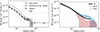 |
Fig. B.1. The Lyα surface brightness profile. Left: The black symbols show the Lyα surface brightness profile extracted within a pseudo-NB of [-600, 600] km/s, with the centroid of the pseudo-NB at the Lyα peak of the target LAE. The grey shadow indicates the error range. The open squares show the Lyα surface brightness profile in Paper I. The dashed line shows the Lyα surface brightness profile in Wisotzki et al. (2018). The grey dashed line shows the PSF profile. Right: The black curve corresponds to the black symbols in the left panel. The red and blue dots with error ranges present the Lyα surface brightness profile extracted by pseudo-NB [0, 600] km/s and [-600, 0] km/s, respectively. These two profiles are multiplied by a factor of 2 for better visualisation. |
All Figures
|
Fig. 1. Surface brightness maps of the median-stacked Lyα emission. Each panel shows the Lyα pseudo-NB in a velocity interval of 200 km/s. The zero velocity corresponds to the peak of the Lyα line. The NBs have been smoothed using a Gaussian kernel of width of 2.3″. The grey contours correspond to Lyα significance levels of 2, 4, and 6σ (dotted, dashed, and solid, respectively). |
| In the text | |
|
Fig. 2. Lyα line profiles at different distances from the central galaxy. The spectra in the left and right columns are derived from the mean- and median-stacked datacubes. Different rows show different radial bins ranging from 1″ (7 kpc) to 8″ (59 kpc). The vertical dashed lines denote the peak of the central Lyα line. The horizontal grey shaded regions show the 1σ error range. |
| In the text | |
|
Fig. 3. As Figure 2, except that here all the mini-datacubes are realigned by the estimated zsys instead of zLyα. |
| In the text | |
|
Fig. 4. Radial evolution of the Lyα peak velocity with respect to the Lyα line of the central LAE. The open circles and squares show the Lyα peak velocity shift in the mean and median stacks (Figure 2). The small symbols connected by dotted lines show the same results extracted with smaller radial bins. The grey horizontal shadow shows the median systemic redshift of the central LAE, as is shown in Figure 3, based on the empirical relations established by Verhamme et al. (2018). The orange and maroon vertical shadows show the maximum radii of the LAHs from previous MUSE (Leclercq et al. 2020; Claeyssens et al. 2019) and KCWI (Erb et al. 2018, 2023) analysis. |
| In the text | |
|
Fig. B.1. The Lyα surface brightness profile. Left: The black symbols show the Lyα surface brightness profile extracted within a pseudo-NB of [-600, 600] km/s, with the centroid of the pseudo-NB at the Lyα peak of the target LAE. The grey shadow indicates the error range. The open squares show the Lyα surface brightness profile in Paper I. The dashed line shows the Lyα surface brightness profile in Wisotzki et al. (2018). The grey dashed line shows the PSF profile. Right: The black curve corresponds to the black symbols in the left panel. The red and blue dots with error ranges present the Lyα surface brightness profile extracted by pseudo-NB [0, 600] km/s and [-600, 0] km/s, respectively. These two profiles are multiplied by a factor of 2 for better visualisation. |
| In the text | |
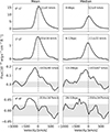 |
Fig. B.2. Same as Figure 2, but for LAEs at 4 < z < 5. |
| In the text | |
Current usage metrics show cumulative count of Article Views (full-text article views including HTML views, PDF and ePub downloads, according to the available data) and Abstracts Views on Vision4Press platform.
Data correspond to usage on the plateform after 2015. The current usage metrics is available 48-96 hours after online publication and is updated daily on week days.
Initial download of the metrics may take a while.