| Issue |
A&A
Volume 690, October 2024
|
|
|---|---|---|
| Article Number | A343 | |
| Number of page(s) | 16 | |
| Section | Extragalactic astronomy | |
| DOI | https://doi.org/10.1051/0004-6361/202451318 | |
| Published online | 23 October 2024 | |
The intrinsic distribution of Lyman-α halos
1
Leibniz Institut für Astrophysik (AIP), An der Sternwarte 16, 14482 Potsdam, Germany
2
Univ. Lyon, Univ. Lyon1, ENS de Lyon, CNRS, Centre de Recherche Astrophysique de Lyon UMR5574, 69230 Saint-Genis Laval, France
3
Aix Marseille Université, CNRS, CNES, LAM (Laboratoire d’Astrophysique de Marseille), UMR 7326, 13388 Marseille, France
4
National Astronomical Observatory of Japan (NAOJ), 2-21-1 Osawa, Mitaka, Tokyo 181-8588, Japan
5
Observatoire de Genève, Université de Genève, Chemin Pegasi 51, 1290 Versoix, Switzerland
6
Department of Astrophysics, Vietnam National Space Center, Vietnam Academy of Science and Technology, 18 Hoang Quoc Viet, Hanoi, Vietnam
Received:
1
July
2024
Accepted:
5
September
2024
Abstract
The emission and escape of Lyman-α photons from star-forming galaxies is determined through complex interactions between the emitted photons and a galaxy’s interstellar and circumgalactic gas. This causes Lyman-α emitters (LAEs) to commonly appear not as point sources but in spatially extended halos with complex spectral profiles. We developed a 3D spatial-spectral model of Lyman-α halos (LAHs) to replicate LAH observations in integral field spectroscopic studies, such as those made with VLT/MUSE. The profile of this model is a function of six key halo properties: the halo- and compact-source exponential scale lengths (rsH and rsC), the halo flux fraction (fH), the compact component ellipticity (q), the spectral line width (σ), and the spectral line skewness parameter (γ). Placing a series of model LAHs into datacubes that reflect observing conditions in the MUSE UDF-Mosaic survey, we tested their detection recoverability and determine that σ, rsH, and fH are expected to have the most significant effect on the detectability of the overall LAH at a given central wavelength and intrinsic line luminosity. We developed a general selection function model that spans a grid of these halo parameters. Using it with a sample of 145 LAHs with measured halo properties observed in the UDF-Mosaic survey, we derived completeness-corrected, intrinsic distributions of the values of σ, rsH, and fH for 3 < z < 5 LAHs. We present the best-fit functional forms of the distributions as well as a σ distribution corrected for instrumental line-spread function broadening, and thereby show the physical line-spread distribution of the intrinsic population. Finally, we discuss possible implications for these distributions for the nature of Lyα emission through the circumgalactic medium, finding that observations may undercount LAHs with extended halo scale lengths compared to the intrinsic population.
Key words: galaxies: evolution / galaxies: high-redshift / galaxies: luminosity function / mass function
Corresponding author; This email address is being protected from spambots. You need JavaScript enabled to view it.
© The Authors 2024
 Open Access article, published by EDP Sciences, under the terms of the Creative Commons Attribution License (https://creativecommons.org/licenses/by/4.0), which permits unrestricted use, distribution, and reproduction in any medium, provided the original work is properly cited.
This article is published in open access under the Subscribe to Open model. This email address is being protected from spambots. You need JavaScript enabled to view it. to support open access publication.
1. Introduction
The Lyman alpha (Lyα) emission line of hydrogen is one of the most effective and commonly used observational tools in the study of galaxy evolution. High-energy photons from young, massive stars ionize neutral hydrogen in a galaxy’s interstellar gas, and when the ionized hydrogen and electron recombine, a Lyα photon is very likely to be emitted (Partridge & Peebles 1967). The emitted Lyα photon can be absorbed or scattered by any neutral hydrogen it encounters, and therefore the Lyα photon’s travel from its origin in the galaxy’s interstellar medium (ISM) through the surrounding circumgalactic medium (CGM) and intergalactic medium will be influenced by the properties of the gas it encounters. The path the photon traverses through these media to the point of observation is determined by complicated radiative transfer pathways that depend on the density, temperature, composition, and kinematic properties of the several phases of intervening gas (Ouchi et al. 2020). Consequently, Lyα emission is a possible tracer of a galaxy’s star formation rate (Sobral & Matthee 2019), characteristics of the baryonic matter in the CGM (Muzahid et al. 2021; Banerjee et al. 2023; Galbiati et al. 2023; Lofthouse et al. 2023), and the ionization of the intergalactic medium (Malhotra & Rhoads 2006; Stark et al. 2010; Matthee et al. 2022; Goovaerts et al. 2023), making the detection of Lyα-emitting galaxies, or Lyman-α emitters (LAEs), a powerful probe of several critical phases of galaxy evolution.
At high redshifts, LAEs and their contributions to reionization are analyzed via population studies, such as with the construction of luminosity functions (LFs; Malhotra & Rhoads 2004; Ouchi et al. 2008; Finkelstein et al. 2012; Drake et al. 2017; Sobral et al. 2018; Herenz et al. 2019; Wold et al. 2022; Thai et al. 2023, which characterize the numerical distribution of LAEs as a function of the Lyα line luminosity in a given redshift epoch (e.g., Johnston 2011) and in a representative volume of the universe: dN = Φ(L)dLdV. Through observation of a population of LAEs at given redshifts, this differential LF can then be evaluated to determine the number density distribution of LAEs as a function of luminosity (or another LAE property) for a given redshift epoch. The form this LF takes is commonly parameterized with the Press-Schechter function (Press & Schechter 1974; Schechter 1976), but it can also be estimated non-parametrically.
Analyses that require knowledge of the intrinsic LAE population – for example, LFs, LAE clustering properties (Herrero Alonso et al. 2023a), and cosmic star formation rate densities (Sobral & Matthee 2019) – require not just measurement of the observed LAEs but also careful consideration of the completeness of the flux-limited observations (see, for example, Drake et al. 2017). The faint LAE population is difficult to consistently detect at high redshifts, especially with spectroscopy, and so luminosity-dependent formalizations of the LF will suffer from a detection bias toward intrinsically brighter sources. Many nonparametric methods for estimating the LF have been developed to address this problem. In this work, we focus on the 1/Vmax estimator (Schmidt 1968; Felten 1976), given generically as
 (1)
(1)
where Vmax, i is the maximum possible volume that the ith observed galaxy can subtend in a survey that detects N galaxies and still be detected by the given observations. To determine a LF, this estimator can then be evaluated for bins of luminosity, but since the generic form is nonparametric, it can be evaluated as a function of other galaxy characteristics as well.
The fractional completeness of galaxy detections is known as the completeness function, or selection function. Differing methods for calculating the selection function can dramatically impact the resulting corrected LAE distribution. We focused on the 1/Vmax method because its nonparametric form for the LF is easily adaptable to include a selection function dependent on the intrinsic luminosity and redshift. However, Herenz et al. (2019) show that in addition to the intrinsic line luminosity of the LAE, the shape of the Lyα halo (LAH) profile can impact the detectability and therefore the measurement completeness of an LAE subpopulation.
Given its complicated escape pathways, Lyα emission is typically not observed tracing the relatively compact stellar population of its host galaxy (Malhotra et al. 2012), but is instead found in a spatially extended LAHs (Matsuda et al. 2012; Momose et al. 2014; Wisotzki et al. 2016; Leclercq et al. 2017; Kusakabe et al. 2022; Guo et al. 2024b; Herrero Alonso et al. 2023b). The Lyα photon’s radiative transfer properties also often create broad, complicated spectroscopic profiles (Verhamme et al. 2006; Erb et al. 2018, 2023; Claeyssens et al. 2019; Blaizot et al. 2023), which can even feature two separate “blue” and “red” peaks, where the observed emission is shifted to lower and higher wavelengths than the Lyα line center predicted by the galaxy’s systemic redshift. Integral field unit (IFU) spectroscopy has proven very successful as a method for probing this 3D spatial and spectral profile, especially with observations from the Multi-Unit Spectroscopic Explorer (MUSE) instrument on the Very Large Telescope (VLT; Bacon et al. 2010, 2017, 2023; Inami et al. 2017; Vitte et al. 2024; Claeyssens et al., in prep.).
At a given redshift and intrinsic line luminosity, the exact spectral shape and spatial distribution of the LAH can significantly affect the rate of LAE detection by effectively spreading the same level of Lyα emission across a broader area, reducing the surface brightness and detected signal-to-noise ratio (S/N). Furthermore, since Lyα escape is determined at least in part by the physical properties of the CGM (e.g., Gronke et al. 2015; Li et al. 2022; Li & Gronke 2022; Blaizot et al. 2023), the distribution of LAH properties can hold valuable information on the typical CGM conditions in different eras of cosmic galaxy evolution. Therefore, the advantage gained by studying the properties and distributions of LAHs is twofold: first, by improving standard techniques for correcting incompleteness in LAE observations, the analysis of LAE populations at high-z can be made more accurate; and second, by uncovering the intrinsic distributions of the physical parameters of LAHs at a given redshift range, we can gain insights into the nature of the CGM, Lyα escape, and other key questions of galaxy evolution.
We have developed a 3D spatial-spectral LAH model that can be used to replicate the observation of an LAH with given halo properties under specific survey conditions. With this model, we can test the relative importance of different halo characteristics to LAH detectability, and thereby produce a grid of models that represent the range of LAH selection functions in a given survey. We applied this to a sample of 3 < z < 5 LAEs studied by Leclercq et al. (2017, hereafter L17) from the Hubble Ultra Deep Field (UDF) Mosaic survey (hereafter “UDF-Mosaic”), conducted with the VLT/MUSE instrument. We used our selection functions and the 1/Vmax completeness estimator to recover intrinsic distributions of the most important LAH parameters, and we discuss their implications for further LAH observations and studies.
The paper is organized as follows. In Sect. 2 we describe our methods for constructing the LAH model and deriving a model’s expected detectability. In Sect. 3 we derive a generalized model for LAH selection functions and apply it to the observed sample from L17. In Sect. 4 we recover the intrinsic parameter distributions for 3 < z < 5 LAHs and discuss their physical implications and future lines of study. We summarize our results in Sect. 5.
In this work, we use CGS flux units, physical distances, and assume a Λ cold dark matter cosmology with Ωm = 0.3, ΩΛ = 0.7, and H0 = 70 km s−1 Mpc−1.
2. Modeling the Lyman-α halo selection function
2.1. The Lyman-α profile
Determining the selection function for LAHs in a given redshift range and for a given observational setup requires the reproduction of a variety of plausible LAH observations under those conditions. For implementation of this procedure in a MUSE IFU cube, we therefore needed to model the LAH emission in three dimensions, as a miniature datacube consisting of a 2D spatial component and a spectral component covering the extent of the Lyα emission line.
2.1.1. Spatial profile
The LAH spatial profile is commonly modeled as a two-component exponential disk (Wisotzki et al. 2016), with one component representing a compact, continuum-like central source, and the second representing a diffuse, extended halo. Previous MUSE observations of LAEs have found this to be an effective model (e.g., Leclercq et al. 2017), and more recent, high-spatial-resolution studies of lower redshift LAEs have confirmed that more simplified spatial models are insufficient (Runnholm et al. 2023). We therefore described the combined profile as
 (2)
(2)
where ΣC(r) (ΣH(r)) describes the radial flux profile of the compact (halo) component, with a total integrated flux of FC (FH), and which we modeled as an exponential disk. The central flux surface brightnesses of the compact and halo components are given by ΣC0 and ΣH0, and rsC and rsH are their exponential scale lengths. We defined the halo flux fraction fH = FH/(FH + FC) in order to describe the relative contribution of each component to the total Lyα flux. Two example spatial profiles with variations on these parameters are shown in panels a and b of Fig. 1.
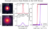 |
Fig. 1. Two example model LAH profiles set in UDF-Mosaic. The left column shows a spatial profile of the model LAH flux, effectively a narrowband image of the Lyα emission, for a model that is spatially relatively compact (panel a) and for a model that is more extended (panel b). The fluxes in each spaxel are log-normalized here to emphasize the distinct shapes. The values of the spatial parameters used for the model are given in the overlaid text. The middle column shows the normalized Lyα spectral profile for a narrow, skewed line (panel c) and for a broader line with no skew (panel d). The right column (panel e) shows the predicted completeness fraction for the compact and extended model LAHs when inserted into UDF-Mosaic observing conditions at different intrinsic fluxes and at a fixed line center of λ0 = 6000 Å. For the range of fluxes Log(FLyα) = − 15 to −19, each model was inserted into a UDF-Mosaic datacube and its S/N measured. For a chosen detection threshold S/Ndet = 5, we then estimated the completeness fraction for each insertion. This is given by the red (compact) and purple (extended) circles and the trend tracked by the solid lines. Dashed lines show error function models of the detectability function, described in Sect. 2.2. Unsurprisingly, the completeness fraction drops rapidly when the intrinsic flux gets low enough to bring the measured S/N below the detection threshold. This behavior can be accurately modeled by an error function, as shown by the dashed lines. This panel also demonstrates the clear effect of the LAH parameters on the expected detectability of the LAE: the spatially compact, narrow-line model is detectable at fluxes almost an order of magnitude fainter than the extended, broad-line model. |
The spatial distribution of the total flux in each component will also depend on its ellipticity, which we measured through the axis ratio, q. We allowed q to vary for the compact component1. The ellipticity of the halo component (qH) was fixed to 1. This is a simplifying assumption that has generally been used for large populations of LAHs observed at high redshift (Wisotzki et al. 2016; Leclercq et al. 2017), where low signals make a proper fitting of the halo ellipticity very difficult, but it will not always be the case for individual LAHs, particularly those exhibiting mergers or substantial gas outflows (Pessa et al. 2024), such as those driven by quasars (Borisova et al. 2016; Arrigoni Battaia et al. 2019). We comment on the potential effects of variable qH and the assumption of qH = 1 in Sect. 3.1.
2.1.2. Spectral profile
The scattering nature of Lyα emission often creates irregular, sometimes double-peaked spectral line shapes, which cannot be adequately replicated with simple Gaussian profiles (Shibuya et al. 2014). Since we were primarily concerned with detectability of the line, we focused on modeling the stronger (and usually redder) peak of Lyα emission (Laursen et al. 2011). Claeyssens et al. (in prep.) find that even when blue peaks are expected to be present, they are unlikely to be detected with MUSE spectral resolution at high redshift. They demonstrate that for a low-z population with blue peak detection rate of 60% in spectra from the Hubble Space Telescope (HST) Cosmic Origins Spectrograph, the rate would drop below 20% with MUSE observations at z > 3, so the blue peak is unlikely to be a strong contributor to the expected observed profiles. Previous MUSE observations and related simulations of Lyα emission suggest the blue-peak-dominated fraction of any sample should be small (Hayes et al. 2021; Kerutt et al. 2022).
Some recent MUSE observations and simulations of LAEs do find significant if small fractions with either blue-peak dominated or double-peaked spectral profiles (Blaizot et al. 2023; Mukherjee et al. 2023; Vitte et al. 2024). From a detectability standpoint, LAEs with a single dominating blue peak will behave functionally very similarly to those with a single red peak, since our spectral model depends on the observed central wavelength of the dominant peak, and not the systemic redshift, for defining the line’s position in the wavelength grid. Lyα spectra with blue and red peaks of comparable flux present a potentially more interesting case, but the inclusion of a second spectral peak would significantly increase the model parameter space to account for a likely small fraction of LAEs. We thus focused on the single-peak case, leaving double peaks to be explored in subsequent work.
The potentially asymmetric profile of a single peak has been modeled as an asymmetric Gaussian (Shibuya et al. 2014), a form used in previous MUSE surveys such as MUSE-WIDE (e.g., Herenz et al. 2017). However, more recent MUSE observations have fit Lyα profiles with a skewed Gaussian function (e.g., Bacon et al. 2023, hereafter B23), which we adopted as well for consistency with the observed halo parameters we used. The functional form of the profile is
 (3)
(3)
Here the critical profile shape parameters are the line width σ, typically measured in km/s, and the skew factor, γ, a dimensionless parameter representing the asymmetry of the line profile. A profile with γ = 0 reduces to a symmetric Gaussian, and as the value of γ increases, the skewness term becomes more dominant, producing a more asymmetric profile. The central wavelength of the profile is given by λ0. Panels c and d of Fig. 1 show the spectral profiles for two specific LAH models, one narrow and heavily skewed, and the other broad and symmetric. More examples of the range of variations in model spectra shapes based on the spectral parameters are shown in Fig. 2.
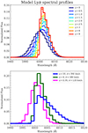 |
Fig. 2. Top: Example model Lyα profiles at the arbitrary and fixed line center λ0 = 6000 Å, with a normalized total line flux and a constant line width σ = 250 km/s. Each color shows a profile with a different skewness factor, γ. The models are resampled to the spectral resolution of VLT/MUSE. Bottom: Three normalized Lyα line profiles determined using the best-fit values of σ and γ for real observed galaxies from B23, demonstrating some of the variety of shapes of observed Lyα spectral profiles. |
2.1.3. Modeling the profile
The spatial and spectral components of the profile combined to contribute six total variable parameters to the LAH model: fH, rsC, rsH, q, σ, and γ. We also varied two line parameters, the intrinsic total LAE flux (log10FLyα) and the central line wavelength (λ0).
For a given set of values of these parameters, we independently modeled the spatial and spectral components of the LAH. First, we used Galfit (Peng et al. 2002, 2010) to convolve the two-component disk profile with a Moffat function (Moffat 1969) representing the point-spread function (PSF) of the observations, using the model spatial parameters and intrinsic line flux. Bacon et al. (2017) measured Moffat profile PSF parameters for UDF-Mosaic, which we have adopted here. We modeled the spatial distribution with the 0.2″ pixel−1 spatial resolution of MUSE, which for the typical halo length scales at 3 < z < 5 fit well in a 51 × 51-pixel spatial array. For each model, we produced such an array, which effectively contained a model narrowband image of the LAH.
We modeled the spectral profile in the observed frame according to the skewed Gaussian form described in Eq. (3), and convolved this profile with the expected broadening of the instrumental line-spread function (LSF). Bacon et al. (2017) determined the LSF through a single-Gaussian model for UDF-Mosaic, according to which the full width at half maximum (FWHM) in Å is
 (4)
(4)
The FWHM evaluated at a given wavelength can then be converted to a Gaussian width and added in quadrature with the “physical” line width, σ0, via  , where σ is the observed line width described in Eq. (3).
We then multiplied each pixel in the 2D spatial profile by the normalized skewed Gaussian spectral profile with given λ0, σ, and γ, distributing the line flux fully in a 3D minicube model of the LAH across the full wavelength MUSE coverage. Here we assumed a constant spectral profile shape across the entirety of the spatial profile, which is not necessarily the case for observed LAHs (Claeyssens et al. 2019; Guo et al. 2024a; Mukherjee et al. 2023). However, these observed spectral variations occur on scales small enough to require substantial stacking or gravitational lensing to confidently observe at high redshift, and can thus be expected to have a small contribution relative to the predominant halo characteristics. As such, the spectral component of our model can be treated as primarily representing the brighter, inner regions of the halo that will dominate the detectability, and the model uses the same values for σ and γ for all spaxels. We then combined this minicube with the variance spectrum and exposure map from the related observations to fully simulate the observing conditions of the model LAH.
2.2. Signal-to-noise estimation and measuring the completeness fraction
To evaluate the detectability of a given LAH emission profile, we used the Line Source Detection and Cataloguing Tool (LSDCat; Herenz & Wisotzki 2017; Herenz 2023), a 3D matched-filtering package for emission line detection developed for IFU observations. LSDCat operates by cross-correlating a 3D emission line template with a continuum-subtracted IFU datacube. For the line template, we used a 3D Gaussian with a spatial width adjusted to the wavelength-dependent PSF and a spectral width of 250 km/s. These template choices have been optimized for Lyα searches with LSDCat and have demonstrated success in previous MUSE surveys (e.g., in MUSE-WIDE; Herenz et al. 2019; Urrutia et al. 2019). After cross-correlation with the cube and its associated variance spectrum, LSDCat returns a S/N cube.
We initially tested the source recovery of the models by inserting LAH models into 51 × 51-pixel UDF-Mosaic-like minicubes at varying levels of intrinsic flux. We ran LSDCat on each minicube and recorded the measured S/N for that model and intrinsic line flux. Setting a threshold level of S/N for detection at S/Ndet = 5, a common observational cutoff for significant detections, we then evaluated the expected completeness fraction fC for each inserted model. This can be seen in panel e of Fig. 1, which shows the expected completeness fraction for the example extended and compact halo models as a function of the intrinsic line flux at a fixed line center of λ0 = 6000 Å. Unsurprisingly, for very bright fluxes, the measured S/N is substantially higher than the threshold, and the expected detectability fraction is essentially 1. At very faint fluxes, the S/N is well below the threshold, and the recovery is essentially 0. In this simple scenario, where we inserted and measured just a single LAH at each flux, the detectability function transitions rapidly from one stage to the other as the intrinsic flux of the models dims and S/N → S/Ndet, with a narrow regime of 0 < fC < 1.
This functional behavior of the completeness fraction has been observed in tests from Herenz et al. (2019) as well, wherein models representing real observed LAHs were inserted and recovered in MUSE-WIDE observing conditions. They also performed multiple insertion tests for each flux level, and so were able to account for variation in the S/N measurement from noise fluctuations across the observed field of view. Since this form is reproduced in both observation-based and analytical models, it is safe to then model the completeness fraction as a function of flux. In the simplest test case we performed above, the transition from fC = 1 to fC = 0 is very narrow, but this assumes a perfect measurement of the S/N, whereas repeated insertion tests of the same models produce a larger spread in the measured recovery function. If the error in measuring the S/N compared to the S/Ndet is assumed to be Gaussian, then the behavior of the resulting detectability function that accounts for the normal distribution of error in the S/N can be described by an error function2. The dashed lines in panel e in Fig. 1 show that this representation closely matches the full-insertion tests.
2.3. Systematic LSDCat insertion and line recovery
Given that the full-model-insertion method described in Sect. 2.2 is well described by an error function, it became possible to replace the time-intensive insertion of the model at every level of intrinsic flux with a more efficient approach: insert the model at a single intrinsic flux, measure the S/N at that level, and then model the S/N, and therefore completeness fraction, for a whole range of possible observable fluxes. This approach is much more practical for attempting to model completeness for a whole LAH population, which may consist of LAHs with a wide range of combinations of halo parameters.
Similarly, it was not necessary to test each model at every possible central wavelength observable by MUSE. With the exception of changing effects of the LSF, the signal measured for a model with a fixed line flux should not change with wavelength, and the LSF effect is generally small relative to the physical line widths, and changes slowly with wavelength. Therefore, the main changes to the S/N measure with wavelength should be expected to depend on the noise properties of the MUSE observations, which has two main drivers: the MUSE sensitivity curve, and the presence of atmospheric skylines. The S/N needed to be measured at a set of wavelengths that accurately accounted for these two factors.
We selected nine separate wavelengths for model LAH insertions: 4930, 5800, 6800, 7116, 7674, 8260, 8563, 9125, and 9193 Å. These wavelengths were chosen to provide a sufficient sampling of the underlying MUSE sensitivity curve (and thus variance spectrum) in relatively skyline-free spectral regions. After sampling the S/N at each of these wavelengths with LSDCat, we interpolated a full S/N curve as a function of wavelength at fixed line flux by using the known variance spectrum for the MUSE UDF-Mosaic survey. This incorporated both the shape of the underlying MUSE sensitivity and the impact of skylines. Then at each wavelength, we modeled fC for a range of intrinsic line fluxes.
This process yielded a selection function for a specific LAH spatial-spectral profile as a function of the intrinsic line flux and the central line wavelength. Examples of this 2D selection function are shown in Fig. 3 for the compact and extended model LAHs depicted in Fig. 1. The selection functions are grids of intrinsic line flux and wavelength, with the value at each grid coordinate the fC expected for that model at the specific flux and wavelength (shown by the color in Fig. 3). Each column in the selection function is the same function as is depicted in panel e of Fig. 1. This immediately demonstrates the impact that variation in the LAH parameters has on Lyα detectability: the compact LAH with a narrow spectral profile is expected to be complete down to almost an order of magnitude fainter intrinsic flux compared to the extended, broad-line halo. To gain a complete understanding of the distribution of LAH properties, it therefore becomes necessary to model this selection function across the range of possible LAH parameters.
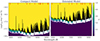 |
Fig. 3. Selection functions for the compact (left) and extended (right) model emitters shown in Fig. 1. The color of each flux-wavelength point on the grid indicates its fC, the detection completeness fraction estimated by the model for UDF-Mosaic. The black and white curves show lines of fC = 0.85 and fC = 0.15. The model in the left column represents a relatively compact LAH, with a halo flux fraction fH = 0.5, a halo scale length rsH = 1.6 kpc, a spectral line width 126 km/s, and a skew parameter γ = 3. The model in the right column is more extended, with a halo flux fraction fH = 0.9, a halo scale length rsH = 5.0 kpc, a spectral line width 316 km/s, and a skew parameter γ = 0. Vertical red lines near the top of the panels indicate the wavelengths where models were inserted into LSDCat. The selection functions predict that these changes will have a substantial effect on the detectability, with the more compact model achieving fC = 1 down to much fainter line fluxes. |
3. A general LAH selection function
3.1. Parameter tests
Determining completeness calculations for the range of possible observed LAHs necessitates a multidimensional grid of selection functions, accounting for variation in each of the six model parameters as well as intrinsic line flux and central wavelength (redshift). Such a grid is potentially very computationally expensive to both generate and analyze. It was thus helpful to consider the relative impact each parameter can have on changes in LAH detectability in order to coarsen or refine the grid resolution in that parameter space accordingly.
We measured this by fixing five of the six LAH parameters to an average value from observed LAHs in MUSE surveys (described in detail in Sect. 3.2), then running the LSDCat recovery test on the observed range of values for the sixth parameter. We tested this in the CANDELS-CDFS-03 field from MUSE-WIDE (Urrutia et al. 2019), a relatively shallow field with well-measured noise properties. The test results are shown in Figs. 4 and 5. We plot the flux at which the modeled completeness fraction fC = 50% as a function of wavelength, yielding a separate “50% curve” for each value of the parameter being tested, shown by different colors. Because the selection function closely resembles an error function, which rapidly changes from 1 to 0, changes in the fC = 0.5 point (F50) will be particularly sensitive to the detectability effects of the changing parameter, making it a useful diagnostic for this test.
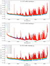 |
Fig. 4. Individual parameter tests for three of the LAH model parameters. Each panel gives the completeness fraction fC = 0.5 as a function of intrinsic line flux and wavelength for a commonly observed range of a given parameter’s values (shown by the colored curves), with the remaining five parameters held fixed at an average value. This demonstrates the variable contribution to the detectability each parameter can make, with γ changing the 50% detection point by only ∼0.05 dex in intrinsic flux, while the q and rsC lead to average changes of 0.08 and 0.13 dex, respectively. |
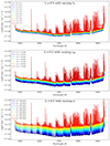 |
Fig. 5. Same as Fig. 4 but for the three remaining LAH model parameters. These parameters have a much more substantial influence on the detectability than the previous set, with fH producing changes of ∼0.12 dex, rsH changing by ∼0.22 dex, and σ generating changes in the fC = 0.5 point of up to 0.5 dex. |
We find the most influential parameters to be the line width, σ, and the halo scale length, rsH (both in Fig. 5). Changes in σ moved the F50 flux by up to 0.5 dex in intrinsic line flux at a given wavelength, and variation in rsH can move F50 by over 0.2 dex. The halo fraction fH and the compact-component scale length rsC had more moderate effects (∼0.12 − 0.13 dex), and the compact ellipticity, q, and the skewness factor, γ, produced relatively small changes in isolation (≤0.1 dex). Here we also tested the possible effects of our assumption of circular halo shape. Fixing average values for the six listed parameters, we checked the F50 curve for qH = 1 and qH = 0.1. This maximal variation produced an average shift of ∼0.07 dex, which is comparable to the effects of γ and q. Given this and the fact that L17, the primary source of our observational constraints, assumed circular halo shapes, we maintained a fixed qH = 1, though we note that more elliptical halos will have slightly improved detectability.
We note as well that this test does not account for possible inherent correlation in the LAH parameters, instead treating them as independent. Consequently, the completeness fractions here as a function of flux should not be considered in absolute terms, but only in the magnitude of the relative change in completeness with the variable parameter. However, even if some correlations between parameters are later discovered, there is initially nothing to indicate that any such connection would cause the detectability properties to change from the smooth, monotonic changes observed in these tests. Potential correlations between halo parameters will be explored further in Sect. 4.4.
3.2. Observational sample: The UDF-Mosaic survey
The main analysis in this work is based on data from UDF-Mosaic (Bacon et al. 2023). The data were obtained between September 2014 and February 2016 with the MUSE/VLT instrument as part of the MUSE consortium guaranteed time observations. The mosaic consists of a grid of nine 10 h observations of 1′×1′ MUSE pointings in the Hubble Deep Field South (HDFS). Overlapping the mosaic is a single 20-h pointing, denoted UDF-10, for a cumulative 30-h of deeper exposure. We note here that though UDF-10 observations contribute to the observed distribution of LAH parameters, the model results in this work will only address the conditions of the mosaic. The UDF data reduction is described in detail in Bacon et al. (2017), and produced a mosaic datacube with a wavelength range of 3750 < λ < 9350, and average resolution of R ∼ 3000, and a spatial resolution of 0.2″ × 0.2″ per pixel. The PSF and LSF characteristics of the observations are well studied, as described in Sect. 2.1.3.
This dataset is convenient for our purposes because the observation depth should be able to probe a range for each LAH parameter, necessary for a comprehensive analysis of the detectability. L17 performed Lyα halo measurements for 145 continuum-faint galaxies in UDF-Mosaic and UDF-10, providing a catalog of rsH, rsC, and halo- and compact-flux measurements from which a halo fraction could be determined. Spectral analysis in B23 provided measures for σ and γ. Distributions of these parameters in the observed sample are shown in Fig. 6. Ellipticity measurements are not commonly available for the L17 sample, especially since many of the continuum-faint sample do not have resolved compact components. In the Lensed Lyman-Alpha MUSE Arcs Sample (LLAMAS), Claeyssens et al. (2022) took advantage of the magnification from gravitational lensing to measure the ellipticity distribution for a comparable LAE sample (Richard et al. 2021). They found half the LAEs consistent with circular compact components (q = 1), with the other half relatively evenly distributed across other values of q. As the lensing magnification provides both improved spatial resolution and access to fainter sources, it is reasonable to use this as a statistically comparable distribution for the ellipticities.
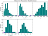 |
Fig. 6. Top: Observed distributions of the compact scale length, halo scale length, and halo fraction in LAHs from the L17 catalog. Bottom: Observed distributions of the line widths and skewness factors for the same sample of LAHs, using the spectral fit results from the B23 catalog. Vertical magenta lines indicate the grid sampling values described in Table 1. |
Grid parameters for UDF-Mosaic.
Prior to fitting the LAH parameters, the L17 sample went through several selection cuts, as described in Sect. 2.2 of that paper. Most selection criteria were for data quality purposes and are unlikely to bias the sample toward or against a particular configuration of halo parameters. The one caveat to note is the removal of LAEs in close pairs (defined as having < 50 kpc projected transverse separation and < 1000 km/s velocity offsets). It is possible that interacting systems have systematically different distributions in one or more of the halo parameters, but determining this would require a large sample of interacting LAEs with well-fit LAH parameters, which is currently not available. The characteristics of this subpopulation will thus be investigated in future work, and the distributions derived in this work will describe the individual LAE population.
3.3. Selection function grids
With the set of LAHs described in Sect. 3.2 as a comparison sample, we designed a parameter grid for which a comprehensive set of selection functions could be generated for LAHs in UDF-Mosaic. The grid design is described in Table 1, and the grid points are shown relative to the observed sample in Fig. 6.
With the potential for a 6D grid to consume substantial computing time, we chose to sample the grid with different step patterns for each parameter based on the parameter’s expected influence on the selection function as measured in the single-variable tests described in Sect. 3.1. We selected the two most influential parameters, σ and rsH, to have finer samplings spanning the observed parameter distributions shown in Fig. 6. Given the distributions show strong peaks at lower values of σ and rsH with long tails at higher values, we opted to sample these parameters in log space, yielding a finer grid where most objects are observed.
We sampled the remaining parameters in linear steps, and with larger step sizes amounting to just two or three sample points per parameter axis. We note as well that for γ, we did not sample the entire observed range, stopping instead at a maximum skewness of γ = 3. As we observe very little change in the selection function for changes in γ beyond γ ⪆ 2 (see Fig. 4), it should suffice for the model to simply test the difference between unskewed (γ ≈ 0) and skewed (γ ⪆ 2) profiles.
Generating a grid to the specifications given in Table 1 produced 2352 individual LAH models and associated selection functions.
3.4. Marginalized selection functions
The relatively coarse sampling of the selection function grid does pose a potential problem for modeling specific LAH profiles that fall between the grid points. This requires a more generalized adaptation of the selection function grid, whereby the selection function for any potential combination of parameter values within the grid ranges can be individually modeled.
To reduce the complexity of the models, we chose to marginalize over the less influential LAH parameters. Selecting q, γ, and rsC as the parameters with the least expected influence on the selection function3, we averaged the completeness curves at each wavelength along the axes of these variables for each set of fixed values of σ, rsH, and fH.
Figure 7 shows a series of example marginalized completeness curves for models with rsH fixed to 5 kpc and fH = 0.9, while varying the line width σ. The marginalization is shown in two possible implementations. First, the dashed curves show flat marginalizations, taking a simple average of completeness curves across models of all values of q, γ, and rsC. However, since we have shown that variations in these parameters can still have some influence on the selection function (see Fig. 4), it would likely produce more accurate results for the marginalization to capture as much of the true distribution of those parameters as possible.
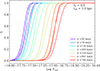 |
Fig. 7. Completeness fraction curves for a series of LAH models that marginalize over the grid axes of the rsC, q, and γ parameters at a fixed central wavelength of λ0 = 6800 Å. These models show fixed values of fH and rsH but variable σ, as indicated by the different colors of the curves. The dashed lines show a flat marginalization, where a simple average is taken over the models of variable rsC, q, and γ at the given fH, rsH, and σ values. The solid lines show the results of a marginalization weighted by the observed distributions of the marginalized parameters (as shown in Fig. 6). This weighted marginalization increases the contribution of models with smaller rsC lengths, resulting in completeness curves that drop off at fainter fluxes. |
We accomplished this via a weighted marginalization, in which the completeness curve average is weighted by the observed distributions of the marginalized parameters as shown in Fig. 6. The primary impact of this is to increase the contribution of models with short rsC values (rsC < 0.5 kpc), which are detected much more frequently and are expected to have the largest impact on detectability out of the remaining three parameters. We weighted the marginalizations along q by the distribution measured by Claeyssens et al. (2022). For the skewness parameter, we weighted by the γ distribution from B23.
The results of this weighted marginalization are shown as solid lines in Fig. 7. The general effect of this marginalization is to shift the completeness curves to fainter fluxes, with the F50 point shifting 0.05−0.1 dex lower in log10FLyα. This makes intuitive sense, given the increased weight to low-rsC models, whose compactness improves their detectability. Of course, weighting the marginalization to observed distributions of the marginalized parameters does potentially induce a bias by under-weighting the contributions of less detectable parameter values (e.g., very extended core scale lengths or very high skewness values). But since we only marginalized the parameters previously determined to have small influences on detectability across their entire observed ranges, such a bias is likely small. LAHs with very high rsC are not so much less detectable than more compact LAHs that missing some will substantially affect the marginalization weights, for example. Thus, we used this set of marginalized models to reduce the parameter space and explore in more detail the distributions of the remaining three LAH parameters.
4. Recovering the intrinsic LAH distribution
4.1. The LAH sample
We used the generalized selection function grid to recover the intrinsic distributions of the line widths, halo scale lengths, and halo flux fractions of 3 < z < 5 LAHs. To begin with, we took a subsample cut of the L17 LAH sample at a S/N level where approximately the full range of observed parameters are still observed. Our fC-based completeness correction can correct a low number of detections to a higher, intrinsic number, but such a correction cannot be applied to zero detections. Ideally, we would make use of as large an observed LAH sample as possible for the best number statistics in assessing the population, but including LAHs at a lower S/N can bias even the corrected distribution, since we could not correct for parameter values that dropped below detection altogether.
We assessed the proper cutoff via S/N diagrams, shown in Fig. 8. Each panel in the figure gives the S/N as a function of σ, rsH, and fH. We needed to select a S/N cut at a level where LAHs were detected across the total observed range of each parameter. For this, we chose S/N = 7, indicated by the dashed red line in Fig. 8. At this approximate level of signal, there is at least one detection even among the rarer LAHs with very high σ or rsH.
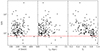 |
Fig. 8. S/N measured from LSDCat for the L17 LAH sample as a function of three LAH parameters: σ, rsH, and fH. Black dots show the individual LAH values, and the dashed red line shows the adopted S/N cutoff at S/N > 7. One feature to note is the S/N behavior of fH, particularly for lower halo fractions. LAHs with low fH are generally not detected with low S/N, despite the detectability advantages for low halo fractions. We discuss this further in Sects. 4.1 and 4.4. |
The one exception is fH, for which no low-S/N LAHs are detected for very low halo flux fractions. There is an apparent anticorrelation between the S/N and fH, with only high-fraction LAHs detected with lower S/N. Given the results of the parameter detectability tests described in Sect. 3.1, which suggest that a lower halo flux fraction increases detectability, this implies that lower-signal low-fH galaxies may simply be intrinsically rarer. This would support findings that lower flux fractions are found with higher intrinsic Lyα luminosities at both low and high redshift (Hayes et al. 2014; Östlin et al. 2014; Wisotzki et al. 2016; Leclercq et al. 2017). Given this, we can take the fH subsample to be complete even if no low-fH LAHs are detected in the sample at S/N = 7.
4.2. The 1/Vmax estimator
The 1/Vmax method is a nonparametric estimator and commonly used completeness metric derived for measuring a galaxy LF (Schmidt 1968; Felten 1976). As a nonparametric method, there is no underlying assumption of distribution shape, so this estimator can be readily adapted to estimate an unknown distribution of galaxies as a function of halo parameters other than luminosity. A generic form of a binned, differential distribution given by the 1/Vmax estimator can be written as
 (5)
(5)
where Xk is a given LAH physical parameter out of a set of k parameters being measured, and each Vmax in the sum is evaluated for the ith out of N galaxies. In this approach, the 1/Vmax, i terms are summed over binned values of Xk, the bin width for which is given by ΔXk.
The term Vmax represents the maximum volume within which a given galaxy can still be detected and included in a given observation (Johnston 2011) and so can be used as a completeness estimator. We used a definition for Vmax modified to account for redshift- and luminosity-dependent detection (Caditz 2016; Herenz et al. 2019):
 (6)
(6)
In this definition, ω is the angular area subtended by the survey, and zmin and zmax are the lower and upper bounds of the redshift range under consideration. For UDF-Mosaic, ω = 9 arcmin2, corresponding to nine 1′×1′ MUSE fields of view. We took zmin = 3 and zmax = 5, corresponding to the redshift range of the L17 sample after our S/N cuts. The dV/dz term is the differential cosmological volume element (Hogg 1999).
The term fc(LLyα, z) represents the selection function, the detection completeness fraction as a function of the intrinsic Lyα line luminosity and the redshift of the observed halo. For each LAH in the L17 sample cut, we used the halo parameters from the L17 and B23 fits to model fc for a specific LAH. We took the total line fluxes measured in L17 for each LAH, converted to the intrinsic Lyα luminosity at the LAH’s measured redshift, and then evaluated the selection function for the model from zmin to zmax in redshift steps equivalent to the MUSE spectral resolution (approximately Δz = 0.001 for the Lyα line center) at fixed intrinsic luminosity.
We then evaluated 1/Vmax for each LAH in the L17 sample cut, integrating the selection function and volume element over the sample redshift range.
4.3. Fitting intrinsic parameter distributions
We evaluated Eq. (6) for binned distributions of σ, rsH, and fH. The results are shown in Fig. 9. Error bars for the 1/Vmax bins account for two major contributions to the uncertainty. First, we included an error term for the Poissonian counting statistics of the 1/Vmax sum (Johnston 2011):
![Mathematical equation: $$ \begin{aligned} \sigma _{\Delta X_k} = \left[\sum _{i=1}^N \left(\frac{1}{V_{\rm max}}\right)^2\right]^{1/2}. \end{aligned} $$](/articles/aa/full_html/2024/10/aa51318-24/aa51318-24-eq8.gif) (7)
(7)
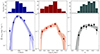 |
Fig. 9. Differential parameter distributions for critical LAH physical characteristics. The panels show distributions for σ (blue), rsH (red), and fH (black), with the top row showing a histogram of input sample LAHs, and the bottom panel the binned 1/Vmax distributions. Individual bins are shown as diamonds with error bars, with the best functional fit shown by the solid or dot-dash lines. Solid lines are lognormal fits, used for the σ and fH distributions, while the rsH distribution was best fit by a broken power law (dot-dash line). The shaded region shows the inter-quartile range of possible fit parameters. The best-fit values are given in Table 2. |
The second major contribution to the error estimation results from errors in binning due to the measurement uncertainties of the halo parameters. We accounted for this with a simple bootstrap resampling, wherein we treated each parameter measurement in the sample as the center of an individual Gaussian distribution with a width equal to the measurement error. Then we resampled each measurement in the sample 1000 times, and performed the same binned 1/Vmax estimation for each of the 1000 new distributions. We took the standard deviation of the 1/Vmax sums in each bin to be the sampling error, and added this error in quadrature with the Poissonian statistics to represent the error in each bin. Typically, the sampling error was on the order of 10% of the counting errors, so the error bars are dominated by the Poissonian term.
The σ and fH distributions are both well fit by a lognormal distribution:
 (8)
(8)
where X represents the mid-bin value for either σ or fH. The free parameters of the fit are the amplitude A, the mean μ, and the standard deviation ν. The best-fit values for these parameters are shown in Table 2. A lognormal function was chosen as the probability distribution that provided the best fit, though a Schechter function also provides a reasonable match.
Best-fit lognormal and smoothly broken power law distributions for halo parameters.
As with the grid construction, we analyzed the 1/Vmax distribution as a function rsH in log space, allowing a finer sampling of the more populated low-r bins. This distribution we fit with a smoothly broken power law, defined as
![Mathematical equation: $$ \begin{aligned} \Phi (R_{\rm H},R_{\rm b},A,\alpha _1,\alpha _2,\Delta ) = A \left(\frac{R_{\rm H}}{R_{\rm b}}\right)^{-\alpha _1} \left\{ \frac{1}{2} \left[1 + \left(\frac{R_{\rm H}}{R_{\rm b}}\right)^{\frac{1}{\Delta }}\right]\right\} ^{(\alpha _1 - \alpha _2)\Delta }. \end{aligned} $$](/articles/aa/full_html/2024/10/aa51318-24/aa51318-24-eq10.gif) (9)
(9)
Here we define RH = log10(rsH), with free parameters Rb (the “break” point between the two power laws), amplitude A, power law indices α1 and α2, and the smoothing parameter Δ. Though we allowed these parameters to fully vary, we obtained the best fits only with a very small smoothing parameter of Δ = 0.003, just above the minimum allowable value of 0.001, resulting in a fit very similar to a simple broken power law.
For each fit, we obtained a confidence interval by repeating the fit over 1000 iterations, varying the values of the input 1/Vmax bins according to a Gaussian resampling with widths equal to the bin measurement errors. The shaded regions shown in Fig. 9 show the interquartile range of possible best-fit parameters from this process. We estimated uncertainty in the fit parameters as well by taking the inter-quartile range of their values from these 1000 perturbed fits. These are also shown in Table 2.
The general forms of the lognormal fits are well constrained, with two caveats: one, the steepness of the drop-offs at low σ or fH could be less constrained due to low-number statistics, and two, the dip as fH → 1 could be consistent with a flat distribution.
The confidence interval for the power law fit shows more features. The bulge around log10(rsH)≈0.8 and some of the other seemingly sharp features in the interval are a result of variation in the free break parameter combined with the fits’ tendencies toward very low smoothness. Compared with the lognormal fits, the edges of the distribution at very low and very high log10(rsH) are less well constrained. However, the downturn at low rsH occurs below what is actually resolvable from the PSF, and so is not a meaningful prediction. At high rsH, it is possible the distribution drops off much more steeply than predicted, but the overall configuration of rising then falling power laws stays the same.
4.4. Implications for the intrinsic LAH population
Next we explored some of the implications of these findings for the intrinsic LAH population at 3 < z < 5, beginning with the flux fraction and halo scale length. We discuss the line width and implications related to the spectral profile in Sect. 4.5. First, we confirm what was suggested above by the parameter tests and S/N distributions: LAHs at 3 < z < 5 with halo flux fractions fH < 0.3 are intrinsically very rare for Lyα luminosities down to 1041.5 erg s−1. As mentioned in Sect. 4.1, this has been hinted at in previous observations that find low-fH galaxies only in small numbers and only at very high Lyα luminosities (e.g., Runnholm et al. 2023, in low-z analogs), an already-rare class of galaxy. But knowing the substantial detectability advantage such galaxies should have, we can now confirm their intrinsic rarity. This also supports previous indications that extended LAHs are essentially ubiquitous around LAEs at this redshift (Wisotzki et al. 2016; Leclercq et al. 2017).
Turning next to the intrinsic distribution of the scale lengths, we find that the most common halo scale length is expected to be around log10(rsH)≈0.7, a scale length of about 5 kpc. This would mean the median halo is extended by factors of 2.5−5 more than the half-light radii measured for galaxies at these redshifts (Bouwens et al. 2004). These scale lengths are not dramatically more common than LAHs with rsH < 4 kpc, but it is notable that they are expected to be the most common scale length in the intrinsic distribution when the observed sample in Fig. 6 shows scale lengths of 1−3 kpc to be more frequent. From the parameter tests, we can expect LAHs with scale length of 2 kpc to be more detectable than those with rsH = 5 by 0.1−0.2 dex in intrinsic flux, a distinction that shapes the difference between the observed and intrinsic distributions.
The distribution drops off sharply at higher scale lengths, though the intrinsic distribution expects LAHs with rsH ≈ 8 kpc to be more common than in the observed distribution by about a factor of 2. The slope of the drop-off is not well constrained, due to the very low number of S/N-sufficient halos, but such extreme extended objects are still expected to be quite rare. Nonetheless, this suggests the importance of the detection of low-surface-brightness galaxies for obtaining a more complete observational sample.
In our initial parameter tests, we operated under the assumption that each variable in the LAH profile can be studied in isolation, independent of the values of the other parameters. There is limited observational testing of this thus far, but L17 (3 < z < 5) and Runnholm et al. (2023, low-z analogs) find little indication that fH correlates meaningfully with the scale length. L17 and Wisotzki et al. (2016) find a significant but relatively weak correlation between the halo and compact-component scale lengths (the Pearson correlation coefficient for the combined sample is ρ = 0.32), albeit with high scatter. So although more extended halo components may be associated with more extended continuum-like components, it is still possible and even common to detect extended halos around more compact continuum-like sources.
Observational tests relating these halo components to physical characteristics of the CGM or host galaxy are similarly limited, due to the small sizes of available samples of LAHs with fit parameters. Here we summarize some results in the literature concerning the halo scale length. With a sample of eight 3 < z < 6 LAEs, Song et al. (2020) find that the halo scale length is significantly driven by the underlying scale length of neutral hydrogen, determined as a fit parameter of the shell radiative transfer model. They find no significant correlation with other shell model parameters. The halo scale length can also correlate with characteristics of the stellar population, such as mass (Zhang et al. 2024), age (Song et al. 2024), and spatial extent of star-forming regions (Rasekh et al. 2022), but the physical connection underlying these correlations must still be explored.
Finally, both simulations and clustering studies suggest that the broad spatial extents of LAHs can be partially explained by contributions from faint LAE satellites (Byrohl et al. 2021; Herrero Alonso et al. 2023b). The L17 sample from which this intrinsic rsH distribution derives was selected to avoid satellites, so this should not be a contributing factor unless the surface brightness contribution from faint satellites below detection limits is significant. The possible impact of such faint satellites will be explored in subsequent work (Kozlova et al., in prep.).
4.5. LSF correction to the line width distribution
Before commenting further on the implications of the intrinsic distribution of spectral line widths, we note that this quantity is not yet measuring a fully physical parameter of the galaxies. In observations, the physical size and shape properties of galaxies are convolved with the effects of observing conditions that alter the observed measurements, spatially through the PSF and spectrally through the LSF. The spatial components such as rsH have already incorporated the PSF information through the Galfit procedure (see Sect. 2.1.3), but spectral components such as σ are still convolved with the LSF.
This LSF was already incorporated into the LAH models used to generate the selection function grid for UDF-Mosaic, such that  . This allowed us to model completeness fractions for observed properties of the L17 LAH sample, for which the σ values fit in B23 give the observed line widths, including the LSF contribution.
For a specific sample of LAHs, such as the L17 subsample, by knowing the emission line wavelengths one can measure the LSF contribution and thereby determine the physical line spread (σ0) for each galaxy. For the recovered intrinsic distribution of σ, however, this is not as straightforward. We could not directly measure the LSF contribution of a galaxy drawn from a predicted distribution, but with our knowledge of the redshift distribution of the observed sample, we could model it.
We took cumulative distributions of the redshifts of the L17 sample and the intrinsic distribution of σ values shown in Fig. 9, which we then normalized into cumulative density distributions. These we sampled one million times, drawing random redshifts and line widths for a mock sample of one million LAHs with statistically similar z and σ distributions.
For this mock sample, since each galaxy was assigned a specific redshift, we could calculate the LSF contribution to its line width and remove it from each mock LAH’s σ value, thereby obtaining σ0 for that mock galaxy. With each mock galaxy deconvolved from its LSF, we took the numerical σ0 distribution and rescaled it to the intrinsic distribution of observed line widths, thereby reconstructing an intrinsic distribution of physical line widths for 3 < z < 5 LAHs.
This reconstructed distribution is shown in Fig. 10, in comparison with the observed intrinsic distribution. Removing the LSF contribution obviously shifts the distribution toward lower σ0 values, but we also found that, while the lognormal distribution described the observed intrinsic distribution well, when applied to the physical σ0 distribution, the fit tended to produce too large a tail at high-σ values. As can be seen in the figure, the lognormal fit is unable to replicate the steeper dropoff at high σ0, instead predicting slightly higher numbers of σ0 > 300 km/s lines in the deconvolved sample than in the uncorrected distribution, an unrealistic scenario.
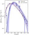 |
Fig. 10. Intrinsic distribution of the line width, σ, in both observed and LSF-corrected forms. Blue diamonds and the blue line and shaded region replicate the distribution from Fig. 9, which is the intrinsic distribution of the observed line widths. This represents a convolution of the physical spread of the line emission with the wavelength-dependent LSF. The purple squares show the intrinsic distribution deconvolved from the LSF, as described in Sect. 4.5. While the observed σ distribution is well fit by a lognormal function, for the LSF-corrected distribution (shown with the solid purple line), this tends to produce a large tail at the high-σ end that is unrealistic for a procedure that reduces the values of σ. A smoothly broken power law function (dot-dash line), as used for the rsH distribution, models the tail end of the distribution more successfully. The LSF deconvolution reduces the σ value of the peak of the distribution from 187 km/s to either 133 km/s (lognormal) or 157 km/s (power law). |
We obtained a superior fit with the smoothly broken power law, previously applied to the rsH distribution. This function is better able to represent the expected steep drop off at high line widths, while still matching the more populated parts of the distribution (see Table 3).
Line width distribution fit parameters.
This choice of functional form does impact the interpretation of the physical line width distribution. Comparing the observed intrinsic fit to the two fits of the intrinsic physical distribution, we find that the peak line width in the LAH population reduces from 187 km/s in the observed intrinsic to 133 km/s (lognormal) or 157 km/s (power law) in the physical reconstruction. The shift of 30 km/s from the observed to physical distributions is very similar to the results of Claeyssens et al. (in prep.), who performed a similar analysis of a sample of lensed LAEs and found an average correction of 20 km/s.
Compared with the spatial parameters discussed above, the Lyα line width has been analyzed more extensively, in both observations and simulations. The intrinsic Lyα line width4 is a key component of the Lyα shell model (Verhamme et al. 2006; Gronke et al. 2015), though its value is often degenerate with other parameters of the model, such as the neutral hydrogen column density. Yang et al. (2017) and Hu et al. (2023) fit Lyα emission from low-redshift LAEs, including “green pea” galaxies, to the shell model, obtaining fit results for the shell model parameters, including the width of the Lyα line. Both are small samples, and both distributions peak at higher line widths (200−250 km/s) than the peaks predicted by the LSF-corrected intrinsic distributions. Subsequent studies of the shell model have noted that it predicts unrealistically broad intrinsic Lyα lines compared to observed Balmer emission Orlitová et al. (2018), indicating that the physically simplistic shell model is not a sufficient representation of the real CGM physics driving LAH spectral properties.
More recent attempts to model Lyα radiative transfer replace the expanding spherical shell model with a clumpy, multiphase medium (Li et al. 2021, 2022). Li & Gronke (2022) compare the two approaches, demonstrating both the existing parameter degeneracies in the shell model and showing that a clumpy model can better fit the broad wings and asymmetric profiles found in observed Lyα spectra without excessively broad intrinsic line widths. Using spatially resolved spectroscopy of 12 z ∼ 2 LAEs from the Keck Cosmic Web Imager, Erb et al. (2023) applied a clumpy, multiphase model to the observed Lyα profiles. They show that the best-fit clump velocity dispersions (one of the six critical parameters in the clumpy model) are found to be ≲150 km/s, which is in line with both the LSF-corrected nebular line widths of their sample and comparable to the peak of our recovered physical line width distribution. In the multiphase clumpy model, intrinsic line widths (prior to radiative transfer) are small, and the velocity dispersion in the neutral gas clumps in the CGM are responsible for broadening the line width in the spectrum. This is a promising connection, and application of this clumpy model to larger LAE samples will further clarify the relationship between the intrinsic distribution of observed line widths and the kinematics of gas clouds in the CGM.
Apart from radiative transfer modeling, many studies have attempted to link Lyα spectral profile characteristics to other observable parameters of LAEs. Yang et al. (2017) find that the width of the observed Lyα red peak (analogous to the spectral feature in our models) correlates with the Lyα escape fraction, and thus anticorrelated with the O32 ratio5, a common diagnostic tracer of ionization in the ISM. This anticorrelation is also observed weakly with a larger sample of 87 low-z LAEs in Hayes et al. (2023), who also observe a weak correlation between O32 and the skewness parameter, but with peak line widths in agreement with the expectation from our distribution (see Fig. 11 in that paper). This could imply a connection between the scattering line width of Lyα emission and the prevalence of ionization channels or ionized outflows in LAEs, although some recent Lyα escape models suggest the photons may be more prone to escape via scattering through higher-density gas than through ionized regions (Almada Monter & Gronke 2024). Ultimately, these are speculative connections in low-z analogs; better comparisons via simulations or high-redshift observations are needed to disentangle the intrinsic line width’s relationship to other characteristics of the halo and galaxy.
There do exist some observational comparisons at higher redshift. González Lobos et al. (2023) find very large (∼500 km/s) line widths associated with strong, large-scale gas outflows in z ∼ 4 LAEs with quasar contributions, but these would be predicted to be an extreme rarity by our intrinsic distribution. L17 also inspected the relationship between the line width and the halo scale length. They measured no overall correlation, but did find that LAHs with rsH < 2 kpc were found to only have narrow lines, while more extended LAHs had line widths across the whole parameter space. Leclercq et al. (2020) measure a significant correlation between line width in the halo component and the halo flux fraction, and a weaker correlation between fH and the ratio of line widths in the halo and the compact component. While not a direct comparison, Claeyssens et al. (2022) also find a significant correlation between the line width and the Lyα 50% light radius. Verhamme et al. (2018) note a correlation between Lyα line width and the line’s velocity offset from systemic redshift among both low- and high-redshift LAEs, and Muzahid et al. (2020) find for z ∼ 3.3 LAEs that this velocity offset also correlates with the host galaxy star formation rate (though this is not found in all studies, e.g., Song et al. 2024). This further hints at connections between the internal dynamics of the host galaxy, the escape pathways available to Lyα emission, the physical extension of the halo gas, and the observed properties of the line. We will explore these possible connections in subsequent work.
5. Conclusions
We have developed a 3D model of the spatial and spectral profiles of 3 < z < 5 LAHs based on six key halo characteristics: the halo and compact exponential scale lengths (rsH and rsC), the halo flux fraction (fH), the compact component ellipticity (q), the spectral line width (σ), and the spectral line skewness parameter (γ). By inserting the model halos into miniature datacubes that mimic specific observations by VLT/MUSE, including the associated variance spectrum, we were able to test detection recovery of different LAH models with LSDCat as a function of the line central wavelength and the intrinsic Lyα line flux. We used this procedure to test the impact on halo detectability of each of the six key parameters in isolation, finding that the line width, σ, the halo scale length, rsH, and the halo flux fraction, fH, influence the line detectability the most.
We used a large sample of 145 LAEs with measured halo spatial properties from the L17 analysis of deep MUSE observations in UDF-Mosaic, reaching LLyα > 41.5 erg s−1. Combining this with spectral properties from the MUSE Hubble Ultra Deep Field Data Release II (Bacon et al. 2023), we had observational measures for the six LAH properties needed for the halo model. We designed a grid of models to span the observed parameter spaces, with finer resolution on the axes of the three most influential parameters. With this spanning grid, we then developed a generalized LAH completeness model that marginalizes over the distributions of the ellipticity, compact scale length, and skewness parameter. This allowed the construction of general selection functions for any LAH based on the input line width, halo scale length, and halo flux fraction.
Taking a subset of the L17 halos for which the subsample was complete for the entire range of observed values for all three key parameters, we reconstructed the intrinsic distributions of these parameters using a version of the 1/Vmax estimator that accounts for variable completeness as a function of intrinsic luminosity and redshift. We present the best-fit functional forms for the intrinsic distributions, finding that the σ and fH distributions are well represented by lognormal functions, while the log10(rsH/kpc) distribution is best fit by a smoothly broken power law with a break at log10(rsH/kpc) = 0.75. We confirm the intrinsic rarity of LAEs with low halo fractions, fH < 0.3, in this redshift-luminosity regime and show that the most common halo scale lengths are toward the middle of the observed distribution (rsH ≈ 5 kpc), though halos with smaller scale lengths are most common in the observations (rsH < 3 kpc). This shows that LAHs tend to be more extended than observed distributions would indicate at first glance, and thus that analyses of LAH populations should carefully account for this less detectable group.
We modeled an LSF deconvolution for the intrinsic σ distribution, developing a distribution that represents the physical line widths without the effects of observational line broadening. This intrinsic physical distribution is best fit by a smoothly broken power law, and it reduced the peak line width from 187 km/s to 157 km/s. We compared these distributions to some basic predictions from shell models, as well as observations from L17 and low-redshift Lyα analogs. There is some evidence of a correlation between the line width and ionization indicators in the interstellar gas, indicating a possible connection between Lyα escape pathways and the physical extension of the emission line. However, this study is still very limited and will have to be expanded upon in subsequent work.
The methods we outline in this work will be applicable to other MUSE surveys, or indeed any contemporary or future IFU observations whose 3D profiles and noise properties can be determined in a similar way. It also provides a framework for modeling and predicting detection results for future Lyα surveys, such as what will be available with the upcoming BlueMUSE instrument, which may be able to detect much larger samples of LAHs in similar observing conditions at lower redshifts.
The axis ratio, q, is related to the other parameters as FC ∝ rsC2ΣC0q; see Peng et al. (2010).
The error function is defined such that  .
.
Though rsC and fH had similar impacts on detectability in the single-parameter tests, observations of fH are more likely to span the full tested range, given the rarity of rsC values greater than 1 kpc as measured from high-resolution HST imaging, and the limitations of measuring low-rsC with a seeing-limited PSF. Therefore, we expect the practical effects of fH to be more substantial.
In radiative transfer studies of Lyα, the intrinsic line width typically refers to the width of the line prior to resonant scattering in the CGM, making this a distinct measure from the observed Lyα line width or even the LSF-deconvolved physical line width described above.
Commonly defined as log10([OIII]4959, 5007/[OII]3727, 3729).
Acknowledgments
We thank the anonymous referee for their helpful suggestions. JP and LW acknowledge funding by the Deutsche Forschungsgemeinschaft, Grant Wi 1369/31-1. TU acknowledges funding from the ERC-AdG grant SPECMAP-CGM, GA 101020943. R.B. and L.W. acknowledge support from the ANR/DFG grant L-INTENSE (ANR-20-CE92-0015, DFG Wi 1369/31-1). Tran Thi Thai was funded by Vingroup JSC and supported by the Master, PhD Scholarship Programme of Vingroup Innovation Foundation (VINIF), Institute of Big Data, code VINIF.2023.TS.108. The authors would like to thank Constanza Muñoz López for helpful consultation on proper parentheses placement.
References
- Almada Monter, S., & Gronke, M. 2024, MNRAS, 534, L7 [NASA ADS] [CrossRef] [Google Scholar]
- Arrigoni Battaia, F., Hennawi, J. F., Prochaska, J. X., et al. 2019, MNRAS, 482, 3162 [NASA ADS] [CrossRef] [Google Scholar]
- Bacon, R., Accardo, M., Adjali, L., et al. 2010, SPIE Conf. Ser., 7735, 773508 [Google Scholar]
- Bacon, R., Conseil, S., Mary, D., et al. 2017, A&A, 608, A1 [NASA ADS] [CrossRef] [EDP Sciences] [Google Scholar]
- Bacon, R., Brinchmann, J., Conseil, S., et al. 2023, A&A, 670, A4 [NASA ADS] [CrossRef] [EDP Sciences] [Google Scholar]
- Banerjee, E., Muzahid, S., Schaye, J., Johnson, S. D., & Cantalupo, S. 2023, MNRAS, 524, 5148 [NASA ADS] [CrossRef] [Google Scholar]
- Blaizot, J., Garel, T., Verhamme, A., et al. 2023, MNRAS, 523, 3749 [NASA ADS] [CrossRef] [Google Scholar]
- Borisova, E., Cantalupo, S., Lilly, S. J., et al. 2016, ApJ, 831, 39 [Google Scholar]
- Bouwens, R. J., Illingworth, G. D., Blakeslee, J. P., Broadhurst, T. J., & Franx, M. 2004, ApJ, 611, L1 [Google Scholar]
- Byrohl, C., Nelson, D., Behrens, C., et al. 2021, MNRAS, 506, 5129 [NASA ADS] [CrossRef] [Google Scholar]
- Caditz, D. M. 2016, ApJ, 831, 50 [NASA ADS] [CrossRef] [Google Scholar]
- Claeyssens, A., Richard, J., Blaizot, J., et al. 2019, MNRAS, 489, 5022 [Google Scholar]
- Claeyssens, A., Richard, J., Blaizot, J., et al. 2022, A&A, 666, A78 [NASA ADS] [CrossRef] [EDP Sciences] [Google Scholar]
- Drake, A. B., Garel, T., Wisotzki, L., et al. 2017, A&A, 608, A6 [NASA ADS] [CrossRef] [EDP Sciences] [Google Scholar]
- Erb, D. K., Steidel, C. C., & Chen, Y. 2018, ApJ, 862, L10 [Google Scholar]
- Erb, D. K., Li, Z., Steidel, C. C., et al. 2023, ApJ, 953, 118 [NASA ADS] [CrossRef] [Google Scholar]
- Felten, J. E. 1976, ApJ, 207, 700 [NASA ADS] [CrossRef] [Google Scholar]
- Finkelstein, S. L., Papovich, C., Ryan, R. E., et al. 2012, ApJ, 758, 93 [NASA ADS] [CrossRef] [Google Scholar]
- Galbiati, M., Fumagalli, M., Fossati, M., et al. 2023, MNRAS, 524, 3474 [NASA ADS] [CrossRef] [Google Scholar]
- González Lobos, V., Arrigoni Battaia, F., Chang, S.-J., et al. 2023, A&A, 679, A41 [NASA ADS] [CrossRef] [EDP Sciences] [Google Scholar]
- Goovaerts, I., Pello, R., Thai, T. T., et al. 2023, A&A, 678, A174 [NASA ADS] [CrossRef] [EDP Sciences] [Google Scholar]
- Gronke, M., Bull, P., & Dijkstra, M. 2015, ApJ, 812, 123 [Google Scholar]
- Guo, Y., Bacon, R., Wisotzki, L., et al. 2024a, A&A, 688, A37 [NASA ADS] [CrossRef] [EDP Sciences] [Google Scholar]
- Guo, Y., Bacon, R., Wisotzki, L., et al. 2024b, A&A, in press, https://doi.org/10.1051/0004-6361/202347958 [Google Scholar]
- Hayes, M., Östlin, G., Duval, F., et al. 2014, ApJ, 782, 6 [NASA ADS] [CrossRef] [Google Scholar]
- Hayes, M. J., Runnholm, A., Gronke, M., & Scarlata, C. 2021, ApJ, 908, 36 [Google Scholar]
- Hayes, M. J., Runnholm, A., Scarlata, C., Gronke, M., & Rivera-Thorsen, T. E. 2023, MNRAS, 520, 5903 [NASA ADS] [CrossRef] [Google Scholar]
- Herenz, E. C. 2023, Astron. Nachr., 344 [CrossRef] [Google Scholar]
- Herenz, E. C., & Wisotzki, L. 2017, A&A, 602, A111 [NASA ADS] [CrossRef] [EDP Sciences] [Google Scholar]
- Herenz, E. C., Urrutia, T., Wisotzki, L., et al. 2017, A&A, 606, A12 [NASA ADS] [CrossRef] [EDP Sciences] [Google Scholar]
- Herenz, E. C., Wisotzki, L., Saust, R., et al. 2019, A&A, 621, A107 [NASA ADS] [CrossRef] [EDP Sciences] [Google Scholar]
- Herrero Alonso, Y., Miyaji, T., Wisotzki, L., et al. 2023a, A&A, 671, A5 [NASA ADS] [CrossRef] [EDP Sciences] [Google Scholar]
- Herrero Alonso, Y., Wisotzki, L., Miyaji, T., et al. 2023b, A&A, 677, A125 [NASA ADS] [CrossRef] [EDP Sciences] [Google Scholar]
- Hogg, D. W. 1999, ArXiv e-prints [arxiv:astro-ph/9905116] [Google Scholar]
- Hu, W., Martin, C. L., Gronke, M., et al. 2023, ApJ, 956, 39 [CrossRef] [Google Scholar]
- Inami, H., Bacon, R., Brinchmann, J., et al. 2017, A&A, 608, A2 [NASA ADS] [CrossRef] [EDP Sciences] [Google Scholar]
- Johnston, R. 2011, A&ARv, 19, 41 [NASA ADS] [CrossRef] [Google Scholar]
- Kerutt, J., Wisotzki, L., Verhamme, A., et al. 2022, A&A, 659, A183 [NASA ADS] [CrossRef] [EDP Sciences] [Google Scholar]
- Kusakabe, H., Verhamme, A., Blaizot, J., et al. 2022, A&A, 660, A44 [NASA ADS] [CrossRef] [EDP Sciences] [Google Scholar]
- Laursen, P., Sommer-Larsen, J., & Razoumov, A. O. 2011, ApJ, 728, 52 [Google Scholar]
- Leclercq, F., Bacon, R., Wisotzki, L., et al. 2017, A&A, 608, A8 [NASA ADS] [CrossRef] [EDP Sciences] [Google Scholar]
- Leclercq, F., Bacon, R., Verhamme, A., et al. 2020, A&A, 635, A82 [NASA ADS] [CrossRef] [EDP Sciences] [Google Scholar]
- Li, Z., & Gronke, M. 2022, MNRAS, 513, 5034 [NASA ADS] [CrossRef] [Google Scholar]
- Li, Z., Steidel, C. C., Gronke, M., & Chen, Y. 2021, MNRAS, 502, 2389 [CrossRef] [Google Scholar]
- Li, Z., Steidel, C. C., Gronke, M., Chen, Y., & Matsuda, Y. 2022, MNRAS, 513, 3414 [NASA ADS] [CrossRef] [Google Scholar]
- Lofthouse, E. K., Fumagalli, M., Fossati, M., et al. 2023, MNRAS, 518, 305 [Google Scholar]
- Malhotra, S., & Rhoads, J. E. 2004, ApJ, 617, L5 [NASA ADS] [CrossRef] [Google Scholar]
- Malhotra, S., & Rhoads, J. E. 2006, ApJ, 647, L95 [NASA ADS] [CrossRef] [Google Scholar]
- Malhotra, S., Rhoads, J. E., Finkelstein, S. L., et al. 2012, ApJ, 750, L36 [NASA ADS] [CrossRef] [Google Scholar]
- Matsuda, Y., Yamada, T., Hayashino, T., et al. 2012, MNRAS, 425, 878 [NASA ADS] [CrossRef] [Google Scholar]
- Matthee, J., Naidu, R. P., Pezzulli, G., et al. 2022, MNRAS, 512, 5960 [NASA ADS] [CrossRef] [Google Scholar]
- Moffat, A. F. J. 1969, A&A, 3, 455 [NASA ADS] [Google Scholar]
- Momose, R., Ouchi, M., Nakajima, K., et al. 2014, MNRAS, 442, 110 [NASA ADS] [CrossRef] [Google Scholar]
- Mukherjee, T., Zafar, T., Nanayakkara, T., et al. 2023, A&A, 680, L5 [NASA ADS] [CrossRef] [EDP Sciences] [Google Scholar]
- Muzahid, S., Schaye, J., Marino, R. A., et al. 2020, MNRAS, 496, 1013 [Google Scholar]
- Muzahid, S., Schaye, J., Cantalupo, S., et al. 2021, MNRAS, 508, 5612 [NASA ADS] [CrossRef] [Google Scholar]
- Orlitová, I., Verhamme, A., Henry, A., et al. 2018, A&A, 616, A60 [Google Scholar]
- Östlin, G., Hayes, M., Duval, F., et al. 2014, ApJ, 797, 11 [CrossRef] [Google Scholar]
- Ouchi, M., Shimasaku, K., Akiyama, M., et al. 2008, ApJS, 176, 301 [Google Scholar]
- Ouchi, M., Ono, Y., & Shibuya, T. 2020, ARA&A, 58, 617 [Google Scholar]
- Partridge, R. B., & Peebles, P. J. E. 1967, ApJ, 147, 868 [Google Scholar]
- Peng, C. Y., Ho, L. C., Impey, C. D., & Rix, H.-W. 2002, AJ, 124, 266 [Google Scholar]
- Peng, C. Y., Ho, L. C., Impey, C. D., & Rix, H.-W. 2010, AJ, 139, 2097 [Google Scholar]
- Pessa, I., Wisotzki, L., Urrutia, T., et al. 2024, A&A, in press, https://doi.org/10.1051/0004-6361/202450547 [Google Scholar]
- Press, W. H., & Schechter, P. 1974, ApJ, 187, 425 [Google Scholar]
- Rasekh, A., Melinder, J., Östlin, G., et al. 2022, A&A, 662, A64 [NASA ADS] [CrossRef] [EDP Sciences] [Google Scholar]
- Richard, J., Claeyssens, A., Lagattuta, D., et al. 2021, A&A, 646, A83 [EDP Sciences] [Google Scholar]
- Runnholm, A., Hayes, M. J., Lin, Y.-H., et al. 2023, MNRAS, 522, 4275 [NASA ADS] [CrossRef] [Google Scholar]
- Schechter, P. 1976, ApJ, 203, 297 [Google Scholar]
- Schmidt, M. 1968, ApJ, 151, 393 [Google Scholar]
- Shibuya, T., Ouchi, M., Nakajima, K., et al. 2014, ApJ, 788, 74 [Google Scholar]
- Sobral, D., & Matthee, J. 2019, A&A, 623, A157 [NASA ADS] [CrossRef] [EDP Sciences] [Google Scholar]
- Sobral, D., Santos, S., Matthee, J., et al. 2018, MNRAS, 476, 4725 [Google Scholar]
- Song, H., Seon, K.-I., & Hwang, H. S. 2020, ApJ, 901, 41 [NASA ADS] [CrossRef] [Google Scholar]
- Song, Z., Reddy, N. A., Chen, Y., et al. 2024, ApJ, 969, 103 [NASA ADS] [CrossRef] [Google Scholar]
- Stark, D. P., Ellis, R. S., Chiu, K., Ouchi, M., & Bunker, A. 2010, MNRAS, 408, 1628 [Google Scholar]
- Thai, T. T., Tuan-Anh, P., Pello, R., et al. 2023, A&A, 678, A139 [NASA ADS] [CrossRef] [EDP Sciences] [Google Scholar]
- Urrutia, T., Wisotzki, L., Kerutt, J., et al. 2019, A&A, 624, A141 [NASA ADS] [CrossRef] [EDP Sciences] [Google Scholar]
- Verhamme, A., Schaerer, D., & Maselli, A. 2006, A&A, 460, 397 [NASA ADS] [CrossRef] [EDP Sciences] [Google Scholar]
- Verhamme, A., Garel, T., Ventou, E., et al. 2018, MNRAS, 478, L60 [Google Scholar]
- Vitte, E., Verhamme, A., Hibon, P., et al. 2024, A&A, submitted [Google Scholar]
- Wisotzki, L., Bacon, R., Blaizot, J., et al. 2016, A&A, 587, A98 [NASA ADS] [CrossRef] [EDP Sciences] [Google Scholar]
- Wold, I. G. B., Malhotra, S., Rhoads, J., et al. 2022, ApJ, 927, 36 [NASA ADS] [CrossRef] [Google Scholar]
- Yang, H., Malhotra, S., Gronke, M., et al. 2017, ApJ, 844, 171 [NASA ADS] [CrossRef] [Google Scholar]
- Zhang, H., Cai, Z., Liang, Y., et al. 2024, ApJ, 961, 63 [NASA ADS] [CrossRef] [Google Scholar]
All Tables
Best-fit lognormal and smoothly broken power law distributions for halo parameters.
All Figures
|
Fig. 1. Two example model LAH profiles set in UDF-Mosaic. The left column shows a spatial profile of the model LAH flux, effectively a narrowband image of the Lyα emission, for a model that is spatially relatively compact (panel a) and for a model that is more extended (panel b). The fluxes in each spaxel are log-normalized here to emphasize the distinct shapes. The values of the spatial parameters used for the model are given in the overlaid text. The middle column shows the normalized Lyα spectral profile for a narrow, skewed line (panel c) and for a broader line with no skew (panel d). The right column (panel e) shows the predicted completeness fraction for the compact and extended model LAHs when inserted into UDF-Mosaic observing conditions at different intrinsic fluxes and at a fixed line center of λ0 = 6000 Å. For the range of fluxes Log(FLyα) = − 15 to −19, each model was inserted into a UDF-Mosaic datacube and its S/N measured. For a chosen detection threshold S/Ndet = 5, we then estimated the completeness fraction for each insertion. This is given by the red (compact) and purple (extended) circles and the trend tracked by the solid lines. Dashed lines show error function models of the detectability function, described in Sect. 2.2. Unsurprisingly, the completeness fraction drops rapidly when the intrinsic flux gets low enough to bring the measured S/N below the detection threshold. This behavior can be accurately modeled by an error function, as shown by the dashed lines. This panel also demonstrates the clear effect of the LAH parameters on the expected detectability of the LAE: the spatially compact, narrow-line model is detectable at fluxes almost an order of magnitude fainter than the extended, broad-line model. |
| In the text | |
|
Fig. 2. Top: Example model Lyα profiles at the arbitrary and fixed line center λ0 = 6000 Å, with a normalized total line flux and a constant line width σ = 250 km/s. Each color shows a profile with a different skewness factor, γ. The models are resampled to the spectral resolution of VLT/MUSE. Bottom: Three normalized Lyα line profiles determined using the best-fit values of σ and γ for real observed galaxies from B23, demonstrating some of the variety of shapes of observed Lyα spectral profiles. |
| In the text | |
|
Fig. 3. Selection functions for the compact (left) and extended (right) model emitters shown in Fig. 1. The color of each flux-wavelength point on the grid indicates its fC, the detection completeness fraction estimated by the model for UDF-Mosaic. The black and white curves show lines of fC = 0.85 and fC = 0.15. The model in the left column represents a relatively compact LAH, with a halo flux fraction fH = 0.5, a halo scale length rsH = 1.6 kpc, a spectral line width 126 km/s, and a skew parameter γ = 3. The model in the right column is more extended, with a halo flux fraction fH = 0.9, a halo scale length rsH = 5.0 kpc, a spectral line width 316 km/s, and a skew parameter γ = 0. Vertical red lines near the top of the panels indicate the wavelengths where models were inserted into LSDCat. The selection functions predict that these changes will have a substantial effect on the detectability, with the more compact model achieving fC = 1 down to much fainter line fluxes. |
| In the text | |
|
Fig. 4. Individual parameter tests for three of the LAH model parameters. Each panel gives the completeness fraction fC = 0.5 as a function of intrinsic line flux and wavelength for a commonly observed range of a given parameter’s values (shown by the colored curves), with the remaining five parameters held fixed at an average value. This demonstrates the variable contribution to the detectability each parameter can make, with γ changing the 50% detection point by only ∼0.05 dex in intrinsic flux, while the q and rsC lead to average changes of 0.08 and 0.13 dex, respectively. |
| In the text | |
|
Fig. 5. Same as Fig. 4 but for the three remaining LAH model parameters. These parameters have a much more substantial influence on the detectability than the previous set, with fH producing changes of ∼0.12 dex, rsH changing by ∼0.22 dex, and σ generating changes in the fC = 0.5 point of up to 0.5 dex. |
| In the text | |
|
Fig. 6. Top: Observed distributions of the compact scale length, halo scale length, and halo fraction in LAHs from the L17 catalog. Bottom: Observed distributions of the line widths and skewness factors for the same sample of LAHs, using the spectral fit results from the B23 catalog. Vertical magenta lines indicate the grid sampling values described in Table 1. |
| In the text | |
|
Fig. 7. Completeness fraction curves for a series of LAH models that marginalize over the grid axes of the rsC, q, and γ parameters at a fixed central wavelength of λ0 = 6800 Å. These models show fixed values of fH and rsH but variable σ, as indicated by the different colors of the curves. The dashed lines show a flat marginalization, where a simple average is taken over the models of variable rsC, q, and γ at the given fH, rsH, and σ values. The solid lines show the results of a marginalization weighted by the observed distributions of the marginalized parameters (as shown in Fig. 6). This weighted marginalization increases the contribution of models with smaller rsC lengths, resulting in completeness curves that drop off at fainter fluxes. |
| In the text | |
|
Fig. 8. S/N measured from LSDCat for the L17 LAH sample as a function of three LAH parameters: σ, rsH, and fH. Black dots show the individual LAH values, and the dashed red line shows the adopted S/N cutoff at S/N > 7. One feature to note is the S/N behavior of fH, particularly for lower halo fractions. LAHs with low fH are generally not detected with low S/N, despite the detectability advantages for low halo fractions. We discuss this further in Sects. 4.1 and 4.4. |
| In the text | |
|
Fig. 9. Differential parameter distributions for critical LAH physical characteristics. The panels show distributions for σ (blue), rsH (red), and fH (black), with the top row showing a histogram of input sample LAHs, and the bottom panel the binned 1/Vmax distributions. Individual bins are shown as diamonds with error bars, with the best functional fit shown by the solid or dot-dash lines. Solid lines are lognormal fits, used for the σ and fH distributions, while the rsH distribution was best fit by a broken power law (dot-dash line). The shaded region shows the inter-quartile range of possible fit parameters. The best-fit values are given in Table 2. |
| In the text | |
|
Fig. 10. Intrinsic distribution of the line width, σ, in both observed and LSF-corrected forms. Blue diamonds and the blue line and shaded region replicate the distribution from Fig. 9, which is the intrinsic distribution of the observed line widths. This represents a convolution of the physical spread of the line emission with the wavelength-dependent LSF. The purple squares show the intrinsic distribution deconvolved from the LSF, as described in Sect. 4.5. While the observed σ distribution is well fit by a lognormal function, for the LSF-corrected distribution (shown with the solid purple line), this tends to produce a large tail at the high-σ end that is unrealistic for a procedure that reduces the values of σ. A smoothly broken power law function (dot-dash line), as used for the rsH distribution, models the tail end of the distribution more successfully. The LSF deconvolution reduces the σ value of the peak of the distribution from 187 km/s to either 133 km/s (lognormal) or 157 km/s (power law). |
| In the text | |
Current usage metrics show cumulative count of Article Views (full-text article views including HTML views, PDF and ePub downloads, according to the available data) and Abstracts Views on Vision4Press platform.
Data correspond to usage on the plateform after 2015. The current usage metrics is available 48-96 hours after online publication and is updated daily on week days.
Initial download of the metrics may take a while.