| Issue |
A&A
Volume 693, January 2025
|
|
|---|---|---|
| Article Number | A36 | |
| Number of page(s) | 24 | |
| Section | Extragalactic astronomy | |
| DOI | https://doi.org/10.1051/0004-6361/202451442 | |
| Published online | 03 January 2025 | |
JWST/NIRSpec insights into the circumnuclear region of Arp 220: A detailed kinematic study
1
University of Trento, Via Sommarive 14, I-38123 Trento, Italy
2
Università di Firenze, Dipartimento di Fisica e Astronomia, via G. Sansone 1, 50019 Sesto F.no, Firenze, Italy
3
INAF – Osservatorio Astrofisico di Arcetri, Largo E. Fermi 5, I-50125 Firenze, Italy
4
Centro de Astrobiología (CAB), CSIC–INTA, Cra. de Ajalvir Km. 4, 28850 – Torrejón de Ardoz Madrid, Spain
5
European Space Agency, c/o STScI, 3700 San Martin Drive, Baltimore, MD 21218, USA
6
Department of Physics, University of Oxford, Denys Wilkinson Building, Keble Road, Oxford OX1 3RH, UK
7
Sorbonne Université, CNRS, UMR 7095, Institut d’Astrophysique de Paris, 98 bis bd Arago, 75014 Paris, France
8
Kavli Institute for Cosmology, University of Cambridge, Madingley Road, Cambridge CB3 0HA, UK
9
Cavendish Laboratory – Astrophysics Group, University of Cambridge, 19 JJ Thomson Avenue, Cambridge CB3 0HE, UK
10
European Space Agency, European Space Research and Technology Centre, Keplerlaan 1, 2201 AZ Noordwijk, The Netherlands
11
Department of Physics and Astronomy, University College London, Gower Street London WC1E 6BT, UK
12
Instituto de Física Fundamental, CSIC, Calle Serrano 123, 28006 Madrid, Spain
⋆ Corresponding author; This email address is being protected from spambots. You need JavaScript enabled to view it.
Received:
10
July
2024
Accepted:
28
October
2024
Abstract
The study of starburst and active galactic nuclei (AGN) feedback is crucial for understanding the regulation of star formation and the evolution of galaxies across cosmic time. Arp 220, the closest ultraluminous infrared galaxy (ULIRG), is in an advanced phase of a major merger with two distinct nuclei, and it shows evidence of multiphase (molecular, ionized, and neutral) and multiscale (from < 0.1 to > 5 kpc) outflows. Therefore, it represents an ideal system for investigating outflow mechanisms and feedback phenomena in detail. Using new JWST NIRSpec IFU observations, we investigated the spatially resolved gaseous (in both ionized and hot molecular phases) and stellar kinematics in the innermost 1 kpc. We decoupled the different gas kinematic components through multi-Gaussian fitting, identifying two multiphase outflows, each associated with one nucleus, with velocities up to ∼1000 km s−1. We also resolved two counter-rotating discs around each nucleus embedded in a larger-scale rotational disk. We compute the total (including ionized, cold, and hot molecular) outflow mass (≈107 M⊙), the mass rate (≈15 M⊙ yr−1), and the energetics (Ėout ≈ 1042 erg s−1) for each nucleus, and we found that the ionized and hot molecular outflowing gas contribute around 2-30% of the total mass and the energy of the outflows, as inferred from the combination of multiwavelength information. We discuss the possible origin of the outflows, finding no compelling evidence to prefer a starburst- or AGN-driven scenario. Regardless of their nature, outflows in Arp 220 propagate in multiple directions from parsec to kiloparsec scales, potentially impacting a significant portion of the host galaxy. This contrasts with isolated systems where outflows typically follow a more collimated path or are limited to the central region of the galaxy and hence do not affect the interstellar medium throughout the entire galaxy. This study highlights the importance of investigating merging systems with multiwavelength facilities, including JWST/NIRSpec IFU, to obtain a comprehensive understanding of feedback mechanisms in galaxy evolution.
Key words: ISM: bubbles / ISM: jets and outflows / ISM: kinematics and dynamics / galaxies: individual: Arp 220 / infrared: galaxies
© The Authors 2024
 Open Access article, published by EDP Sciences, under the terms of the Creative Commons Attribution License (https://creativecommons.org/licenses/by/4.0), which permits unrestricted use, distribution, and reproduction in any medium, provided the original work is properly cited.
This article is published in open access under the Subscribe to Open model. This email address is being protected from spambots. You need JavaScript enabled to view it. to support open access publication.
1. Introduction
Ultraluminous infrared galaxies (ULIRGs) with infrared (IR) luminosities LIR > 1012 L⊙ are among the most luminous objects in the local Universe. Their extreme IR luminosity is due to the combination of high star formation rate (SFR) and active galactic nuclei (AGN) activity, coupled with a high dust content, which intercepts the UV photons emitted from either hot young stars or AGN and reemits them at longer wavelengths (Soifer et al. 1984; Sanders & Mirabel 1996; Lonsdale et al. 2006; U et al. 2012 and references therein).
In the starburst-quasar evolutionary scenario (e.g., Sanders et al. 1988; Hopkins et al. 2008), ULIRGs are thought to represent a rapidly growing phase of massive galaxies. Within this framework, the merger of gas-rich galaxies triggers a phase of vigorous star formation (SF), fueling the growth of supermassive black holes (SMBHs) and the eventual onset of AGN activity. As the merger progresses, powerful outflows generated by both starburst and AGN winds shape the galactic environment, influencing subsequent SF and black hole accretion with feedback mechanisms (e.g., Di Matteo et al. 2005; Silk 2013).
Galactic outflows are expected to be more important at high redshift (z ∼ 1 − 2) during the peak of the cosmic SF and SMBHs accretion (Madau & Dickinson 2014), and hence where the feedback mechanisms may be maximized (e.g., Brusa et al. 2015; Talia et al. 2017; Perrotta et al. 2019; Kakkad et al. 2020; Cresci et al. 2023). Remarkably, recent observations have revealed some similarities between local ULIRGs and distant starbursts at redshift z ∼ 2 (e.g., Arribas et al. 2012; Hung et al. 2014; Bellocchi et al. 2022; McKinney et al. 2023) and they highlight the importance of understanding the outflow phenomena occurring in local ULIRGs. In fact, the proximity of these sources allows for more detailed observations that are characterized by angular resolution and signal-to-noise ratios higher than those focusing on more distant galaxies.
Several studies have demonstrated the presence of multiphase (ionized, neutral, and molecular) gas outflows in ULIRGs (e.g., Sturm et al. 2011; Bellocchi et al. 2013; Veilleux et al. 2013; Arribas et al. 2014; Feruglio et al. 2015; Cazzoli et al. 2016; Fluetsch et al. 2021; Perna et al. 2021; Lai et al. 2022; Bohn et al. 2024). In this work, we focus on the closest prototypical ULIRG, Arp 220, where evidence of multiphase outflows has already been obtained from several multiwavelength observations (e.g., Arribas et al. 2001; McDowell et al. 2003; Colina et al. 2004; Perna et al. 2020; Wheeler et al. 2020; Lamperti et al. 2022; Ueda et al. 2022).
Arp 220 is located at a distance of ∼78 Mpc, and has an IR luminosity of log (LIR/L⊙) = 12.2 (Pereira-Santaella et al. 2021), and a stellar mass of log (M*/M⊙)∼10.8 (U et al. 2012). It is a late-stage merger containing two compact (< 150 pc), highly obscured nuclei (east and west) separated by ∼370 pc (1″) that dominate the IR luminosity (e.g., Scoville et al. 2007). The two nuclei are sites of intense SF, with SFR ∼200 − 250 M⊙ yr−1 (e.g., Nardini et al. 2010; Varenius et al. 2016) and extremely high SFR surface densities ΣSFR ∼ 103 − 104 M⊙ yr−1 kpc2, from radio and far-IR (FIR) observations (e.g., Barcos-Muñoz et al. 2015; Pereira-Santaella et al. 2021). There is still no convincing direct evidence for the presence of AGN activity in either of the two nuclei (see Perna et al. 2024 and references therein).
This paper presents a kinematic examination of the nuclear region of Arp 220 observed with the Integral Field Spectrograph (IFS) unit of the Near Infrared Spectrograph (NIRSpec) instrument on board the James Webb Space Telescope (JWST) (Jakobsen et al. 2022; Böker et al. 2022) collected as part of the JWST/NIRSpec IFS Guaranteed Time Observations (GTO) survey: Resolved structure and kinematics of the nuclear regions of nearby galaxies (program lead: Torsten Böker). Our goal is to investigate the spatially resolved gaseous and stellar kinematics in the innermost 1 kpc of Arp 220, and better understand the feedback processes affecting this ULIRG system.
This paper is organized as follows. Section 2 presents the NIRSpec observations and data reduction. Sections 3 and 4 present the spectral fitting analysis and the results through the characterization of the spatially resolved kinematics of the atomic and molecular gas and the identification and study of the different structures found in the central 1.5 × 1.8 kpc of Arp 220. In Sect. 5, we describe the main properties of the interstellar medium (ISM). In Sect. 6, we discuss our results and a comparison with the literature. Finally, Sect. 7 summarizes our conclusions. Throughout this work, we assume Ωm = 0.286 and H0 = 69.9 km s−1 Mpc−1 (Bennett et al. 2014). With this cosmology, 1″ corresponds to 0.368 kpc at the distance of Arp 220.
2. Observation and data reduction
Arp 220 was observed using the JWST/NIRSpec instrument in IFS mode (Böker et al. 2022), as part of the JWST observing program 1267 (PI: D. Dicken), on March 6, 2023. These NIRSpec observations were combined in a single proposal with independent MIRI GTO observations of the same target.
The dataset comprises two distinct pointings, each employing the first four positions of the medium cycling dithering pattern with 15 groups per integration and one integration per exposure, using the NRSIRS2RAPID readout pattern. The first set is centered at the midpoint between the coordinates of the western (W) and eastern (E) nuclei, while the second set is offset by approximately 1″ toward the northwest to encompass the Hα and [N II] emission shell (Lockhart et al. 2015; Perna et al. 2020). Each set has a total integration time of 933 seconds and utilises three high-resolution (R ∼ 2700) configurations: G140H/F100LP, G235H/F170LP, and G395H/F290LP, covering wavelength ranges of 0.97–1.82 μm, 1.66–3.05 μm, and 2.87–5.14 μm, respectively. However, this paper focuses solely on the first two configurations, as our objective is to study the kinematics of the emitting gas, with its strongest transitions occurring at wavelengths below 2.4 μm.
The data reduction of Arp 220 observations is described in detail in Perna et al. (2024). Here we summarize the relevant information. We used the JWST pipeline v1.8.2 with CRDS context 1063. A patch was included to correct some important bugs that affect this specific version of the pipeline; 1/f noise and outliers were corrected following the approaches described in Perna et al. (2023) and D’Eugenio et al. (2023), respectively. The combination of the exposure for the eight dither positions was done with a drizzle weighting method that allowed us to sub-sample the detector pixels (Law et al. 2023), resulting in cube spaxels with a size of 0.05″ (corresponding to ∼20 pc/spaxel) and covering a field of view (FoV) of 5″ × 4″. The absolute astrometric registration was performed using ALMA high-resolution maps of millimeter continuum emission, as described in Perna et al. (2024). The final data cubes showed strong “wiggles”, sinusoidal modulations caused by the undersampling of the point spread function (PSF). We corrected these artifacts by applying the methodology described in Perna et al. (2023).
Figure 1 shows the three synthetic narrow-band images generated from the reduced data cube of Arp 220 obtained for the brightest emission lines in the wavelength range covered by NIRSpec. The positions of the W and E nuclei are marked for visual purposes. This figure illustrates the quality of NIRSpec data and provides a preview of the intricate gas kinematics within the innermost regions of Arp 220.
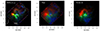 |
Fig. 1. Three-color emission line images of Arp 220. The emission line maps are obtained integrating the continuum-subtracted data-cube around [Fe II] 1.257 μm (left), Paα (center), and H2 1–0 S(1) 2.122 μm (right) in the velocity ranges −400 km s−1 < v < −200 km s−1 (blue), −200 km s−1 < v < 200 km s−1 (green) and 200 km s−1 < v < 400 km s−1 (red), with respect to the median value between zE* and zW*, zm = 0.0181. The red crosses mark the position of the two nuclei. |
3. Spectral fitting analysis: Stellar and gas components
In this section we describe the spectroscopic analysis carried out to study the kinematics and morphology of the nuclear region of Arp 220. We show in Fig. 2 the integrated spectra of the E and W nuclei up to 2.4 μm, extracted from a circular aperture of radius 3 spaxels (corresponding to 0.15″) centered at the positions defined in Perna et al. (2024), reported in Table 1. The spectra are shown in the rest-frame, according to the systemic redshift of each nucleus: z = 0.01840 for the E and z = 0.01774 for the W (Perna et al. 2024, see also Sect. 3.3). The spectra show many hydrogen recombination lines, including Paschen (Pa) and Brackett (Br) transitions, but also many forbidden iron lines ([FeII]), and roto-vibrational transitions of molecular hydrogen (H2). This allowed us to study the physical and kinematic properties of the gas in different phases. The CO absorption bandheads in the spectral ranges 1.5–1.7 μm and 2.2–2.4 μm are prominent, and can be used to measure the stellar kinematics.
 |
Fig. 2. Arp 220 W and E nuclear spectra. The spectra were extracted from a circular aperture of radius 3 spaxels (corresponding to 0.15″) and are reported in units of flux density as a function of rest-frame wavelength. Red dashed vertical lines identify H2 lines; black dashed lines identify ionized gas transitions. Gold-filled areas mark the position of the main CO stellar absorption lines. |
Coordinates and systemic redshift of the two nuclei of Arp 220 from Perna et al. (2024).
The analysis is divided into three steps: the first is the modeling and the subtraction of the stellar continuum, the second is a preliminary fit of the emission lines to build a model that can be used to study the integrated properties of each emission line. The third step is the disentangling of the different kinematic components associated with the most prominent emission lines. These three steps are described in detail in the following sections.
3.1. Modeling of the stellar continuum
To fit the stellar continuum, we used the penalized pixel-fitting routine (pPXF) (Cappellari & Emsellem 2004; Cappellari 2017) to convolve stellar spectra templates with a Gaussian velocity distribution. We did not attempt to extract the Gauss–Hermite terms h3 and h4, since the quality of our data is not sufficient to obtain this information from the fit (see also e.g., Cappellari et al. 2009; Engel et al. 2011; Crespo Gómez et al. 2021). We binned spaxels together using the Voronoi binning scheme of Cappellari & Copin (2003), to achieve a minimum S/N. We established a target minimum S/N = 30 per wavelength channel for each bin (following e.g., Belfiore et al. 2019). We used the MARCS stellar population synthesis templates (Gustafsson et al. 2008) to model the stellar continuum; these templates cover the wavelength range 0.96–20 μm with a constant spectral resolution Δλ/λ = 20 000. We also adopted a third-order multiplicative and additive polynomials to better reproduce the spectral continuum shape. To improve the quality of the fit, we included in the total model the most prominent emission lines (see Table 2) parameterized with two Gaussian components.
Fit emission lines. Vacuum wavelengths are taken from Perna et al. (2024).
We conducted separate fits for the cubes G140H and G235H, with the latter restricted to wavelengths below 2.4 μm, to avoid spaxels affected by the NIRSpec detector gap. Wavelengths falling within the gap in G140H were appropriately masked during the fit procedure. Fig. 3 shows the fit with pPXF of the spectra extracted from the W and E nuclei, highlighting the most important features in absorption (black dashed lines) to constrain stellar kinematics. We note that the pPXF best fits does not perfectly reproduce the observed spectra. However, this does not affect our goal: we do not require a realistic model of the stellar populations in Arp 220, we only need an accurate stellar continuum model and a measurement of the stellar kinematics.
 |
Fig. 3. Arp 220 W and E nuclear spectra with pPXF best-fit models. The CO absorption features are in the 1.5–1.7 μm band (upper panel) and 2.2–2.36 μm (bottom panel). Black and green curves respectively refer to the data and the model of the W nucleus spectrum. Brown and gold curves respectively refer to the data and the model of the E nucleus spectrum. Black dashed vertical lines indicate the position of the main CO absorption lines. |
After constructing the total model, we subtracted the model of the continuum from the cube spaxel by spaxel, rescaling the modeled continuum emission obtained in each Voronoi bin to the median flux of the observed continuum in each spaxel. In this way, we obtained a cube containing only the contribution of the emission lines.
3.2. Multi-Gaussian emission line fit
After the subtraction of the continuum, we smoothed each wavelength map of the cube (i.e., image generated with a spectral pixel wide synthetic filter) with a Gaussian having a dispersion of 1 spaxel (i.e., 0.05″), to enhance the S/N. We then performed separate spectral fits for the atomic and molecular gas line groups listed in Table 2 since each gas phase may be dominated by different kinematic components, as illustrated in Fig. 1 (see also e.g., May & Steiner 2017; Perna et al. 2024). All lines within each group were simultaneously fitted using one, two, or three Gaussian components. We tied the velocity v and the velocity dispersion σ of each Gaussian component among all lines of the group, while the fluxes are left free to vary. Then, we chose the number of Gaussian components for each spaxel by performing a Kolmogorov-Smirnov (KS) test on the distribution of the residuals with N and N + 1 components to define the minimum number of components required to provide an acceptable fit in each spaxel (Marasco et al. 2020). Consequently, the number of Gaussian components is not based on a physical model but it is constrained on just a statistical analysis; a detailed, physical decomposition is presented in Sect. 4.
Figure 4 shows the three moment maps calculated on the whole modeled line profile (consisting of either one, two, or three Gaussians) of the brightest emission lines: H2 1 − 0 S(1) 2.122 μm, Paα, and [Fe II] 1.257. For each transition, we masked spaxels with S/N < 3. These maps allowed us to identify the different kinematic and morphological components of the system, traced by ionized and molecular gas, and described in Sect. 4.
 |
Fig. 4. Moment maps of hot molecular gas (H2 1-0S(1), top) and ionized gas (center: Paα, bottom: [Fe II] 1.257 μm). The moment-1 was computed with respect to zm = 0.0181. An S/N cut of three on the flux of each emission line was applied to the maps. The black “+” symbols mark the position of the E and W nuclei. White contours represent the edges of the masks described in Sect. 4. |
3.3. Systemic velocity
Following Perna et al. (2024), we determined the redshift of the two nuclei from the centroid of the atomic hydrogen lines in the nuclear spectra. The systemic velocities correspond to zEgas = 0.01840 ± 0.00001 and zWgas = 0.01774 ± 0.00001. We also computed the redshift from the stellar continuum model, finding zE* = 0.0183 ± 0.0002 and zW* = 0.0179 ± 0.0003, slightly different from the redshift found for the gas, but still consistent within the errors (see Table 1).
In this work, the large-scale (> 100 pc) stellar and gas kinematics maps are derived by using as a reference the redshift reported in Perna et al. (2020), which corresponds to the median value between zE* and zW*, zm = 0.0181 (e.g., Fig. 4). This redshift allows us to obtain a symmetric stellar velocity gradient, associated with the kiloparsec-scale disk also identified with optical and cold molecular line tracers (see Perna et al. 2020 and references therein). In contrast, the small-scale motions of the ionized and hot molecular gas around the E or W nucleus are measured relative to the zero velocity inferred from zEgas and zWgas, respectively.
4. Spectral fitting analysis: Separating rotations and outflows components
The morphology and kinematics of the nuclear region of Arp 220 are quite complex. Figs. 1 and 4 reveal a superposition of circum-nuclear and large-scale disks as well as multiple outflows that have already been observed in optical and submillimeter tracers (e.g., Scoville et al. 2017; Perna et al. 2020; Lamperti et al. 2022; Ueda et al. 2022). Emission lines often display multipeak and asymmetric spectral profiles, requiring the use of multiple Gaussian components for modeling. Conventional methods usually employed to separate a disk from an outflow structure across the entire galaxy (e.g., based on velocity or velocity dispersion criteria; Tozzi et al. 2021; Venturi et al. 2021), may not be straightforward for Arp 220. Hence, in this work we opted for an alternative approach, focusing on individual regions where the separation of distinct kinematic components is facilitated by dedicated criteria and by the high spatial resolution of NIRSpec data. In particular, we first selected and modeled the most easily distinguishable outflow components, subtracted them, and then gradually move on to the more complex ones.
Our method consists of three steps. The first is the identification of a region with specific morphology and/or kinematics, and hence the construction of a spatial mask to isolate it. We then fitted all spaxels within the selected region with N Gaussians, where N represents the number of the kinematically distinct components we wanted to characterize. As the fit of a complex line profile is subject to degeneracy, the value N is quite critical and depends on the detectability of the morphological and kinematic features we aim to describe. We considered in our model the most intense transitions of the atomic (Paα) and molecular gas (H2 1 − 0 S(1) 2.122 μm, hereafter H2 unless otherwise specified) in the G235H cube. We also included in the fit the HeI 1.869 μm and He 1.870 μm lines since they can contaminate the profile of Paα (see, e.g., Fig. B.3 in Perna et al. 2024). We fitted together the transitions of atomic and molecular gas assuming for each line the same v and σ and varying the fluxes. As we show in the next sections, this is a reasonable assumption for this system. In the second step, we defined a criterion to isolate an outflow among the components identified in the mask. Then, we constructed a model cube containing only the isolated component, used for further analysis presented in the following sections.
This three-step process is iterative, implying that each time we aimed to characterize a specific feature, we initially created a mask and then fitted a new model on the residual cube built by subtracting all previously detected and isolated components. The criteria used to define all masks and outflow components are introduced in the next sections (Sects. 4.1–4.4).
Fig. 5a illustrates the masks for all the identified outflow regions. They encompass a conical outflow launched by the E nucleus (i.e., the southeast outflow, SEO hereinafter), an hourglass-shaped outflow originating from the W nucleus (HGO), and a northwestern bubble (NWB). There is another feature of particular interest that affects just a few spaxels and is therefore not reported in the figure: a compact outflow observed in the W nucleus mainly in the ionized phase (WNO). In the next subsections, we provide detailed analyses of each identified region.
 |
Fig. 5. Arp 220 outflow regions. (a): Composite view of the isolated outflow regions: southeast outflow (red), hour-glass outflow (blue), northwest outflow (green). (b): Channel map between −650 and −300 km s−1 in the H2 transition with respect to the systemic redshift of the E nucleus. The white curve indicates the edges of the SEO mask. (c): Sum of channel maps < − 200 and > 200 km s−1 in the H2 transition with respect to the systemic redshift of the W nucleus. The white curve indicates the edges of the HG region. (d): Sum of H2 and Paα channel maps between −800 and −450 km s−1 with respect to the systemic redshift of the E nucleus. The white curve indicates the edges of the NWB region. |
4.1. Southeast conical outflow from E nucleus
Figure 5b shows H2 emission in the velocity range [ − 650, −300] km s−1 with respect to the systemic velocity of the E nucleus. In this figure, a high-velocity conical region situated southeast of the E nucleus is clearly visible (demarcated by white lines). This region has also elevated velocity dispersion (> 150 km s−1), as shown in the moment-2 maps of both ionized and hot molecular gas in Fig. 4, hence indicating the presence of an outflowing component.
We selected the region with enhanced flux in the [ − 650, −300] km s−1 map (red area in Fig. 5a) and, within this region, fitted both the ionized gas and the molecular gas with three Gaussian components to model: 1) the high-velocity gas, 2) the rotating disk at a large scale that covers the entire FoV, and 3) the emission from the small circum-nuclear disk around the E nucleus. Among these three Gaussian components, we assigned the most blueshifted to the outflow. The flux, the velocity and the velocity dispersion of the SEO in H2 and Paα are reported in Fig. 6. Since we associated only one Gaussian component to the outflow, the velocity and the velocity dispersion is the same for both ionized and hot molecular gas. The velocity varies between −100 km s−1, observed close to the nucleus and at the edges of the cone, and −400 km s−1 at larger distances (∼400 pc). High velocity dispersions (up to 200 km s−1) are observed in the center of the conical outflow and close to the nucleus, while at the edges of the cone σ is about two times lower.
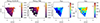 |
Fig. 6. SE conical outflow flux and velocity maps. From left to right: flux of H2 and Paα lines, velocity, and velocity of the Gaussian component attributed to the SE outflow. The velocities are relative to the systemic velocity of the E nucleus. Red crosses indicate the positions of the two nuclei. Green asterisks in the first panel indicate the spaxels presented in Fig. 7. |
Figure 7 shows the spectra of the hot molecular (top) and ionized gas (bottom) extracted from three spaxels within the conical outflow; specifically near the E nucleus, at the center, and at the edge of the cone. In all spaxels, we observe a prominent wing extending toward negative velocities; this wing is reproduced by a Gaussian component with v < −250 km s−1, which we associated with the SEO (red curves in the figure). We also note that the SEO emission is more prominent and contributes more to the total line profile in the hot molecular phase than in the ionized one, especially in the off-nuclear regions. Figure 7 also shows that our multi-Gaussian approach is capable of simultaneously reproducing the profiles of ionized and hot molecular gas, hence supporting the validity of our assumption about the presence of a mixed, multiphase ISM in each kinematic component.
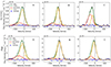 |
Fig. 7. Spectra extracted from the SE outflow cone. The solid black curves represent the line profiles of H2 (top) and Paα (bottom) extracted from the spaxel close to the E nucleus (A), in the central part of the cone (B), and at the edge of the collimated outflow (C), as labeled in Fig. 6. The multi-Gaussian fits are depicted by dashed orange curves for the disk components and solid red curves for the outflow component. The total model for the disk is shown as a solid orange curve, and the combined model for both disk and outflow is displayed in green. The blue dots indicate the residuals. The velocities are computed with respect to the systemic velocity of the E nucleus. |
As explained in Sect. 4, our approach consists of an iterative process: the best-fit model component attributed to the SEO is subtracted spaxel by spaxel from the original data cube before performing new fits to characterize the remaining kinematic structures observed in the NIRSpec data. This method helps in reducing the fit degeneracy.
4.2. Hourglass outflow from the W nucleus
As shown in Fig. 1, both the ionized and molecular gas exhibit a shell-shaped morphology at high redshifted (v > 200 km s−1) velocities in the region north of the W nucleus. Additionally, the hot molecular gas shows a blueshifted shell-like structure in the region southwest of the same nucleus. The blue- and redshifted gas forms an ‘hourglass’ (HG)-like shape, compatible with an outflow launched from the W nucleus. This structure is even clearer in Fig. 5c, showing the sum of H2 spectral channel maps at v < −200 km s−1 and v > 200 km s−1 (with respect to the systemic velocity of the W nucleus), used to define our mask (white contours in the figure).
Within the HG region, we fitted simultaneously the hot molecular and the ionized gas using three Gaussian components, taking into account the large- and small-scale gas rotations as well as the outflow. To assign a Gaussian component to the HG outflow (HGO), we discarded the components with absolute velocities < 180 km s−1. Among the remaining ones, we attributed to the outflow the component with highest absolute velocity. The threshold (180 km s−1) represents a compromise: with a smaller velocity threshold, we would have included in the outflow also part of the rotational disk at larger scales; with a higher value, we would have missed part of the contribution of the outflow.
Figure 8 shows the flux, velocity and velocity dispersion of the gas component attributed to the outflow. The flux is dominated by the hot molecular gas over the ionized one. The velocity field is rather symmetrical with respect to the W nucleus and varies between −300 and 400 km s−1. The highest observed velocity is located to the east in the redshifted shell, corresponding to an increase in molecular gas emission line flux. It is unclear whether this high-velocity gas is still part of the HGO, or whether it may represent a redshifted counterpart of the conical SE outflow associated with the E nucleus (Sect. 4.1).
 |
Fig. 8. HG outflow flux and velocity maps. From left to right: flux of H2 and Paα lines, velocity, and velocity dispersion of the Gaussian component attributed to the HG outflow. The velocities are relative to the systemic velocity of the W nucleus. Red crosses indicate the positions of the two nuclei. Green asterisks in the first panel indicate the spaxels presented in Fig. 9. |
Figure 9 shows the spectra extracted from three spaxels within the HG region (A, B, C in Fig. 8), to illustrate our fitting procedure and the separation of the kinematic components. The red curve refers to the component attributed to the outflow, while the orange curves refer to the other components used for the fit. We note that the line profiles in this region are very broad and multiple components are needed to model them. Nevertheless, despite differences in the line profiles of the hot molecular and ionized gas at specific positions, the multi-Gaussian fits successfully reproduce these profiles, confirming the reliability of our fit decomposition.
 |
Fig. 9. Spectra extracted from the HG outflow region. The solid black curves represent the line profiles of H2 (top) and Paα (bottom) extracted from the spaxels marked in Fig. 8. The red curve refers to the HG outflow. Orange curves identify the additional components used for the fit (orange dashed curves). The combined model is displayed in green. The velocities are computed with respect to the systemic velocity of the W nucleus. |
4.3. Northwest bubble
We identified a large scale bubble in the north west of the NIRSpec FoV, mostly visible in the [Fe II] transitions (Fig. 1). Figure 5d displays the sum of spectral channel maps at v < −450 km s−1 (with respect to the systemic velocity of E nucleus) of Paα and H2. We created the mask for the NW bubble (NWB) by selecting those spaxels with enhanced flux in these velocity channels, excluding the region around the W nucleus (white curve in the figure). This nuclear region was already included in Sect. 4.2, but since its outflow kinematics are slightly different from those of the HG outflow, this region is discussed in Sect. 4.4.
The emission that contributes to the line profiles in this mask comes from the bubble and the large-scale rotating disk. Consequently, we fitted the emission lines with two Gaussian components. No specific boundaries on velocity and velocity dispersion were used during the fit. We assigned the most blueshifted component to the outflow. This Gaussian component also exhibits a higher velocity dispersion with respect to the one associated with the disk.
Figure 10 shows the flux, velocity and velocity dispersion of the gas component attributed to the outflow. In this region, the fluxes of Paα and H2 are very similar, except in the area closest to the W nucleus, where the ionized phase dominates. The velocity ranges between −100 and about −450 km s−1, with velocities dispersion > 150 km s−1.
 |
Fig. 10. NW bubble flux and velocity maps. From left to right: flux of H2 and Paα lines, velocity, and velocity dispersion of the Gaussian component attributed to the outflow. The velocity is referred to the E nucleus. Red crosses indicate the positions of the two nuclei. Green asterisks in the first panel indicate the spaxels presented in Fig. 11. |
Figure 11 shows the fit of Paα and H2 in three spaxels extracted from the bubble. The black dashed curve represents the spectra from the original cube, highlighting the component (red-shaded area) attributed to the HGO that we have already isolated and subtracted. The red curves represent the NWB component, while the orange curves correspond to the other components used in the fit. In all panels, the nature of the Gaussian components is clear: the outflow component is blueshifted and broader than the disk component.
 |
Fig. 11. Spectra extracted from the NW bubble region. Line profiles of H2 (top) and Paα (bottom) are shown at the position of the three spaxels labeled in Fig. 10. The black dashed curves represent the spectra from the original cube, highlighting the contribution attributed to the HGO (red-shaded area) that we have already isolated and subtracted; the black solid lines represent the spectra fitted to identify the NW bubble. The red Gaussian profiles identify the isolated NW bubble, while orange profiles identify the rotating disk component. The combined model is displayed in green. The velocities are computed with respect to the systemic velocity of the E nucleus. |
4.4. Compact outflow from the W nucleus
There is another kinematic feature in the W nuclear region that has not been isolated yet. It is a nuclear outflow (WNO) that is visible in the ionized gas phase (see also Perna et al. 2024). However, it affects just a few spaxels and cannot be isolated in the moment maps (Fig. 4) nor in the velocity channel maps (e.g., Fig. 1). Therefore, once all the features described before (i.e., the SEO, the HGO, and the NWB) have been subtracted, we fitted the residual cube with two components to model the WNO and the perturbed rotating gas (i.e., large-scale rotation over the entire FoV, or small-scale rotating nuclear discs).
We attributed to the WNO the components with σ > 150 km s−1 within a radius of 0.4″ (150 pc) around the nucleus. In the more external regions, we associated both the components to the perturbed rotating gas. Figure 12 shows the three moments of the components attributed to the perturbed disk in H2 and Paα (top and central panels) and of the WNO (bottom panels). The WNO kinematics are characterized by blueshifted velocities up to −200 km s−1 and a velocity dispersion of ∼150 − 200 km s−1.
 |
Fig. 12. Moment maps of the large-scale rotating disk and the W nuclear outflow. Top and middle panels: moment-0 (left), moment-1 (center), and moment-2 (right) maps of H21-0S(1) (top) and Paα (middle) of the Gaussian components attributed to the perturbed disk. The black-dashed line in the velocity maps show the large-scale disc mean kinematic major-axis (PA = 45°). Bottom panels: Paα moments maps of the Gaussian components attributed to the W nuclear outflow. Velocities are referred to zm in the first two rows. Velocity in the zoom-in inset is referred to the systemic velocity of the W nucleus. |
Figure 13 shows the spectrum extracted from a random spaxel (marked in the bottom panel of Fig. 12) to illustrate the fit decomposition for the ionized and hot molecular gas phases. The differences in the line profile of the two gas phases are evident: the broad, blueshifted wing that is observed in Paα is not observed in the molecular gas.
 |
Fig. 13. Spectrum extracted from the WNO. Line profiles of H2 (left) and Paα (right) extracted from a spaxel labeled in the bottom panel of Fig. 12). The two component fits are represented by the dashed orange (disc component) and red (outflow component) curves; the combined model is displayed in green. The velocities are computed with respect to the systemic velocity of the W nucleus. |
4.5. Perturbed rotating disk
The moment maps of hot molecular and ionized gas shown in Fig. 4 already suggested a large-scale rotation pattern, although strongly affected by several outflow features. These additional kinematic components were isolated and subtracted in Sects. 4.1, 4.2, 4.3 and 4.4. The fitting procedure used to separate the compact nuclear outflow (WNO) component from the rotating disk is described in the previous section (Sect. 4.4). After the subtraction of the components associated with the WNO, we assigned to the perturbed rotating gas all the components having σ < 200 km s−1. In fact, the components with higher velocity dispersion might represent residuals of outflowing gas that we did not model in the previous steps. Figure 12 (top and central panels) shows the moment maps of the isolated perturbed rotating gas, with contributions from both circum-nuclear discs in the vicinity of the E and W nuclei and the large-scale disk. The Moment-1 velocities are defined with respect to zm = 0.0181, which is more appropriate for the kiloparsec-scale disk (see Sect. 3.3).
We observe a symmetric velocity gradient with respect to the E nucleus, with velocities from −250 km s−1 (northeast) to +250 km s−1 (southwest). The Moment-1 map in the northwest part of the FoV is instead disturbed due to the non-perfect subtraction of HGO and NWB contributions. Moreover, significant deviations from a large-scale rotational patter are also observed in the vicinity of the W nucleus: this is due to the presence of a small-scale disk surrounding the W nucleus (see also e.g., Scoville et al. 2017). We calculated the position angle (PA)1 of the major kinematic axis of the large-scale disk by fitting the Moment-1 map of Paα and for H2 with the FIT KINEMATIC PA code (Cappellari et al. 2007; Krajnović et al. 2011), obtaining 51 ± 7° and 39 ± 7°, respectively. In Sect. 4.6, we use the average of these two values to construct the position-velocity (PV) diagram.
The Moment-2 of the perturbed rotating disk reaches values up to 150 km s−1, significantly lower than in the moment 2 map obtained before the subtraction of the outflowing features (Fig. 4). Moreover, the kinematics of Paα are more perturbed compared to that of the hot molecular gas, as also seen in Armus et al. (2023). Figure 14 shows three single-spaxel spectra extracted from the HG region (B), the SEO cone (C), and an overlapping region of the HG and NW bubble (D) (See Fig. 12). After the subtraction of the outflow components, the line profiles are now rather symmetrical; the second component used in the fit procedure (red dashed curves) either is much fainter than the first component, or shows similar velocity shifts and line widths. Therefore, the attribution of both components to the disk is well justified.
 |
Fig. 14. Spectra extracted from the kiloparsec-scale disk. Line profiles of H2 (top) and Paα (bottom) at the position of the three spaxels labeled in Fig. 12. The black dashed curves represent the spectra from the original cube, highlighting the contribution attributed to the HGO and SEO (red-shaded area) that we have already isolated and subtracted; the black solid lines represent the spectra fitted to identify the large-scale disk. The red dashed curves show the components associated with the disk model. The total disk model is shown with a solid red curve. Velocities are computed with respect to zm. |
4.6. Stellar kinematics
Figure 15 presents the stellar kinematics maps obtained with pPXF. In particular, they are created from the analysis of the G235H cube, which is less affected by dust attenuation than the G140H cube and shows more prominent CO stellar absorption features in the wavelength range 2.2–2.4 μm (Fig. 2). In Fig. A.1 we show that the maps derived from the G235H and G140H gratings are consistent. As shown in the inset panel of Fig. 15, the stellar velocity field of Arp 220 presents two nuclear discs rotating in opposite directions separated by 1”, with a velocity offset of ∼120 km s−1 (see also Wheeler et al. 2020; Sakamoto et al. 1999). The stellar velocity dispersion is higher in the nuclear positions, and then decreases throughout a region crossing the two nuclei, in correspondence with the bright elongated region observed in the Paα Moment-0 map (Fig. 12). Moreover, in the E nucleus, the velocity dispersion increases toward the east, while in the W nucleus it increases in the south direction. In the outermost regions north of the two nuclei, the velocity dispersion reaches about 200 km s−1, consistent with the values found in Perna et al. (2020).
 |
Fig. 15. Stellar kinematics maps. Top panels: Stellar velocity (left, in the frame zm) and velocity dispersion (right). Bottom panels: Stellar velocity (left) and velocity dispersion (right) around the two nuclei shifted with respect to the rest-frame velocity of each nucleus. Black dashed lines refer to the major axis of the two nuclei (W: PA = 257°, E: PA = 45°). Light blue dashed line refers to the axis of HG outflow (PA = 13°). |
In the next two sub-sections we compare the stellar and gas kinematics making use of PV diagrams.
4.6.1. Stellar and gas kinematics around the W nucleus
In this section we compare the gas and stellar kinematics around the W nucleus. We constructed a PV diagram of both the ionized gas and the hot molecular gas (Fig. 16), centered on the W nucleus with a PA ∼ 257 ± 6° directed along the major axis of rotation of the circumnuclear stellar disk calculated with the FIT KINEMATIC PA code (dashed black line in Fig. 15). We set the zero velocity at the redshift of the W nucleus ( ). The ionized gas (upper panel) reaches blueshifted velocities higher than those of the hot molecular gas (bottom panel). The stellar component (black star symbols in the plots) follows the kinematics of ionized gas, while it appears to rotate faster than the hot molecular gas.
 |
Fig. 16. Position-velocity diagram for ionized gas (top) and hot molecular gas (bottom) of W nucleus with positions varying along the disk major axis (PA = 257°, left, with positive distances toward west), the disk minor axis (PA = 347°, center, with positive distances toward north); and HG outflow axis (PA = 13°, right, with positive distances toward southwest). Black stars represent the stellar velocity. The zero-velocity refers to |

In the PV diagram along the circumnuclear disk’s minor axis (PA ∼ 347 ± 6°), the ionized outflow (WNO), discussed in Sect. 4.4, is evident. It extends about 0.3″ from the W nucleus and exhibits velocities reaching up to 600 km s−1 both in the blue- and redshifted sides. However, this feature is not detected in the hot molecular gas, probably due to the dissociation of the H2 molecules or, more in general, to different physical conditions (e.g., in terms of magnetic field and electron density in the outflowing gas; see, e.g., Kristensen et al. 2023).
We also constructed a PV diagram along the axis of the HG outflow (PA = 13°, left panel of Fig. 16), which is not exactly perpendicular to the axis of rotation of the circumnuclear disk. Ionized gas dominates the emission within 0.5″ radius of the W nucleus, and decreases considerably at larger distances; instead, the H2 emission is more diffuse. The high blue- and redshifted velocities spans a range of −200 km s−1 < v < 300 km s−1 at a distance of about 1.5″ (600 pc), delimiting the HG outflow. To summarize, around the W nucleus we found 1) a relatively good match between stellar and gas kinematics, 2) a strong nuclear ionized outflow (blue and redshifted) in addition to the HG outflow.
4.6.2. Stellar and gas kinematics around the E nucleus
Figure 17 shows the PV diagram along the major axis of the stellar rotational disk centered at the position of E nucleus (PA = 45°). Since it was not possible to decouple the contribution of the small-scale disk surrounding the E nucleus from the large-scale disk, the major axis of the small-scale disk was assumed to be aligned with the one of the large-scale disk computed in the previous subsection. We set the zero velocity at the redshift of the E nucleus ( ).
).
 |
Fig. 17. Position-velocity diagrams of large-scale rotational disk centered on the E nucleus. In the left panels, the positions vary along the mean kinematic major axis (PA = 45°), with positive distances toward south-west. In the right panels, the positions vary along the minor axis (PA = 135°), with positive distances toward north-west. The upper panels show the PV diagrams of Paα, while the lower panels show PV diagrams of H2 1-0 S(1). Black stars identify the stellar kinematics. The zero-velocity refers to |

The stellar component follows the rotation of the gas around the nucleus. In the ionized gas (Fig. 17, top), a peak in the flux is observed at redshifted velocities ∼250 km s−1, representing a bright clump at the north of the E nucleus (NE cluster in Perna et al. 2024), not observed in the hot molecular phase.
A blueshifted nuclear outflow is observed in both the hot molecular gas (bottom) and the ionized gas (top), reaching velocities of about −600 km s−1. This emission forms the vertex of the SE conical outflow we isolated in Sect. 4.1.
5. ISM properties
5.1. Attenuation
We used the emission-line ratios [Fe II] 1.644/1.257, Brγ/Paβ and Paα/Paβ as attenuation diagnostics. We measured the line ratios from each spaxel, and scaled them to calculate E(B − V) as follows (Domínguez et al. 2013):
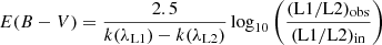 (1)
(1)
where L1 and L2 are the lines used for the diagnostic, and k(λL2) and k(λL1) are the values of the reddening curve evaluated at L1 and L2 wavelengths. The intrinsic ratios are taken respectively from Bautista & Pradhan (1998), Hummer & Storey (1987) and from CLOUDY (Ferland et al. 2017) assuming a temperature of 104 K and a density ne = 100 cm−3. We adopted the Calzetti et al. (2000) attenuation law valid between 0.12 to 2.2 μm with Rv = 4.05 estimated from optical-IR observations of four starburst galaxies.
Figure 18 shows the dust attenuation maps estimated from the different emission line ratios with a cut in S/N (> 3) for each line, as AV = 4.05 × E(B − V). The attenuation AV varies between 2 and 14 mag, reaching higher values in the E nucleus (consistent with Perna et al. 2024) and lower values in the outer part of the FoV. The three attenuation maps computed with different line ratios are consistent. The attenuation computed from Eq. (1) integrating the fluxes in the central region (where the S/N of the faintest line Brγ > 3) varies less than 20% between the three attenuation diagnostics. These values are also consistent with the stellar attenuation computed by Engel et al. (2011) through the K band, Av = 6 − 12, while our values are a factor 2-3 higher than their estimates through Paα/Brγ.
 |
Fig. 18. Dust attenuation maps from the[Fe II] 1.257 μm to [Fe II] 1.640 μm ratio (left), Brγ/Paβ (middle) and Paα/Paβ (right). |
5.2. Star formation
We derived the SFR from the Paα dust corrected luminosity by summing the contribution of the perturbed rotating discs as defined in Sect. 4.5, excluding all the outflow components. We used the Paα flux corrected for the dust attenuation spaxel per spaxel derived from the Paα/Paβ, resulting in an increase of the Paα flux of a factor ∼2.2, and we followed Reddy et al. (2023):
![Mathematical equation: $$ \begin{aligned} \mathrm{SFR} (\mathrm Pa\alpha )\left[\mathrm{M}_{\odot }\, \mathrm{yr}^{-1}\right] = \mathrm C(Pa\alpha ) \times \mathrm L(Pa\alpha ) \left[\mathrm{erg\,s}^{-1}\right] \end{aligned} $$](/articles/aa/full_html/2025/01/aa51442-24/aa51442-24-eq6.gif) (2)
(2)
where C(Paα) = 3.90 × 10−41 assuming an upper mass cutoff of the IMF of 100 M⊙ and a solar metallicity. We derived a total SFR of ∼8 M⊙ yr−1. The value of SFR found with the recombination line is significantly lower than ones computed in a similar area with FIR and radio data (∼200 M⊙ yr−1, from Varenius et al. 2016 and Pereira-Santaella et al. 2021), possibly indicating that a large fraction of the SF is totally blocked by dust at NIR wavelengths (Giménez-Arteaga et al. 2022; Perna et al. 2024).
The largest contribution to the emission of recombination lines comes from the elongated region located between the two nuclei with relatively faint H2 emission. In Fig. 19a we show the ratio of the total Paα flux to the total H2 flux, which peaks up to 30 north of the E nucleus and drops to values less than one in the outermost regions. We also observed blobs in which the ratio reaches values of approximately two (in log: 0.3–0.4 from Fig. 19a); one of the largest is located about 1″ west of the W nucleus. These blobs lie along a preferential NS direction, probably along a filament or dust lane where SF is more intense.
 |
Fig. 19. Maps of ionized over hot molecular gas ratio and SF surface density. (a) Spatially resolved flux ratio log(Paα/H2) computed from the total profile of the two lines. (b): Surface density map of the SFR inferred from Paα after subtraction of the outflowing components. |
Figure 19b shows the SFR surface density map, ΣSFR. The ΣSFR is highest in the elongated region between the two nuclei (10–40 M⊙ yr−1 kpc−2), while the other regions have value < 1 M⊙ yr−1 kpc−2. The ΣSFR calculated over the entire FoV (∼1.5 kpc × 1.5 kpc) has a value of ∼3 M⊙ yr−1 kpc−2. Similar values are reported in a sample of ULIRGs studied with VLT/SINFONI (Piqueras López et al. 2012), ranging between 0.4 and 2 M⊙ yr−1 kpc−2. Based on FIR measurements, the SFR surface densities of the nuclear region of Arp 220 reaches values higher than 103 M⊙ yr−1 kpc−2. As discussed in Perna et al. (2024), this discrepancy may be explained taking into account different factors: the high obscuration caused by the dust, the different scale times of SF that the two bands (FIR and NIR) trace and to the possible presence of AGN that is completely obscured in the NIR. Typical star formation surface density values computed in radio band in ULIRGs are 50 − 1000 M⊙ yr−1 kpc−2 in the nuclear region (< 1 kpc2), and 5 − 500 M⊙ yr−1 kpc−2 on scales of few kiloparsec (Lucatelli et al. 2024).
5.3. Outflows properties and energetics
In this section, we estimate the outflow energetics of the molecular and of the ionized gas. To estimate the mass of the outflowing gas in the hot molecular phase, we followed Scoville et al. (1982) and Mazzalay et al. (2013):
 (3)
(3)
where Mout, H2 is the hot molecular mass traced by H2, DL is the luminosity distance, and A2.2μm is the attenuation at 2.2 μm. This equation assumes thermalized gas conditions and T = 2000 K, with a population fraction in the (ν, J) = (1, 3) level of f(1, 3) = 0.0122. We applied Eq. (3) for each spaxel and then we summed over the region of the spatially resolved outflows (namely, the SEO, the HGO, the NWB, and the WNO) to compute the total masses. We computed A2.2μm as shown in Sect. 5.1 through Paα/Paβ, since it involves the lines with higher S/N among the line ratios considered. However, when computing the properties of the outflow in the spaxels where we could not infer the attenuation due to low S/N < 3 in Paα and Paβ, we assumed AV corresponding to the mean value in the defined region.
To compute the ionized outflow mass, we adopted the simplified model by Genzel et al. (2011), valid for case B recombination of fully ionized gas with T ∼ 104 K. The mass of outflowing gas is given by
 (4)
(4)
where LHα is derived from LPaα corrected for attenuation assuming a theoretical ratio Paα/Hα = 0.11, and ne is the electron density.
The determination of the ionized gas mass is significantly influenced by ne, which can span a few orders of magnitude, from 102 to 104 cm−3 (e.g., Villar Martín et al. 2014; Perna et al. 2017; Förster Schreiber et al. 2019; Isobe et al. 2023). We derived the electron density through the line ratio [Fe II] 1.677 μm/[Fe II] 1.644 μm. We fitted the integrated spectrum around the lines of interest considering in the model also the Br11 line, since it is blended with [Fe II] 1.677 μm. Since the latter line is very faint at spaxel level, we integrated the spectra over the individual outflow regions SEO (Fig. 6), HGO (Fig. 8), NWB (Fig. 10), and WNO (Fig. 12, bottom panels), to infer average electron densities for each outflow. Moreover, due to the low S/N of [Fe II]1.677, we considered the total profile of [Fe II] 1.677 μm and 1.644 μm, without distinguishing the contribution of non-outflowing components. We obtained electron densities in the range log (ne/cm−3) ≈3 − 4 from the relation in Koo et al. (2016).
We found that the region with the highest electron density is the WNO ( cm−3). For the HGO, we found
  cm−3. We also integrated the spectrum and computed the electron density in both the red- and blueshifted region of the HG outflow, separately. We found
  cm−3 for the redshifted and a 3σ upper limit of 5 × 104 cm−3 in the blueshifted part. In the SEO and in the NWB the emission of [Fe II] 1.677 μm is not detected, resulting in upper limits on the electron density: < 1.7 × 104 cm−3, and < 1800 cm−3, respectively. All the inferred values are reported in Table 3.
Properties of the high-velocity molecular and ionized outflows.
The ne estimates through the [Fe II] transitions are higher (a factor ∼10–100) than those found from the [S II] doublet in the optical band with MUSE (170 cm−3, Perna et al. 2020). This may indicate a gas stratification in the nuclear regions of Arp 220, with [Fe II] emission, having higher critical density (Nc ∼104 cm−3), tracing the densest part of the ISM, and [S II] (Nc ∼ 103 cm−3) tracing the more diffuse gas. It is worth noting that using a constant density of ne ∼ 102 cm−3, as the one derived by Perna et al. (2020) using [S II], could lead to an overestimation of the gas masses and the energetics, because this line emission likely traces partially ionized gas with lower densities (Davis et al. 2011; Revalski et al. 2022). On the other side, our estimation of the ne from [Fe II] doublet comes only from the nuclear (WNO) and the most compressed regions (HGO), where the faint [Fe II] 1.677 μm line is detected. Thus, this electron density may not be representative of the density in the full FoV. Therefore, we chose to estimate the outflow properties with electron density estimations from both [Fe II] and [S II] that may represent reasonable lower and upper boundaries.
For each isolated outflow in Sect. 4, we determined the mass outflow rate, Ṁout, at a given radius Rout by using the assumptions of a constant outflow speed vout and spherical (or multiconical) geometry. Following Lutz et al. (2020), we have
 (5)
(5)
where C is a factor that depends on the outflow history. We adopted a constant mass outflow rate (C = 1). We calculated the radius from the flux maps of each outflow. In particular, we measured Rout as the maximum extension from the corresponding nucleus. Specifically, for the HGO and WNO, we calculated the distances from the W nucleus, while for the SEO and NWB we calculated them from the E nucleus. We associated the NWB to the E nucleus, in order to have a more conservative estimation of the mass outflow rate. This choice is also motivated by the fact that the outflows launched by the W nucleus are oriented along the NS direction (Sect. 4.2), while the one of the E nucleus is along the SE direction. Moreover, the 100 pc scale molecular outflow launched by the E nucleus and traced by CO (Wheeler et al. 2020) is similarly oriented along the SE-NW direction.
We used the definition of the outflow velocity in Rupke & Veilleux (2013) as
 (6)
(6)
where vbroad and σbroad are the velocities relative to the systemic velocity of the nucleus from which the outflow originates, and the velocity dispersion of the outflowing component, respectively. We computed the outflow velocities as the flux-weighted average of the outflow velocity of each spaxel. We assigned the standard deviation of the values in that region as the uncertainty on vout. The properties of the ionized and molecular gas outflows for the analyzed regions are reported in Table 3.
The outflow masses and the mass outflow rates of the hot molecular gas vary from 700 M⊙ in the SEO to 2000 M⊙ in the HGO, and from 6 × 10⁻⁴ M⊙ yr−1 for the NWB to 1 × 10⁻² M⊙ yr−1 for the HGO, respectively. For the ionized gas, the outflow mass varies from a minimum of 5 × 10³ M⊙ for the SE outflow to a maximum of 9 × 10⁴ M⊙ fort the WNO, calculated with the density from the [Fe II] doublet. The highest mass outflow rate of ionized gas is measured in the WNO with a value of 8 M⊙ yr−1, estimated using the density from the [S II], while the lowest is measured in the NWB with a value of 0.4 M⊙ yr−1.
We also computed the kinetic energy and the kinetic power of the outflow as  and
and  , respectively. We found that the contribution to the energetics of the ionized outflow is about 1–3 orders of magnitude higher than that of the hot molecular gas, depending on the density used in the computation. The kinetic energy of the ionized gas outflows ranges between 1.7 × 1054 erg for the SEO to 4.6 × 1054 erg for the WNO, estimated with [S II].
5.4. Three-dimensional outflow modeling
To measure the geometrical parameters of SEO, HGO and the NWB outflows we used the modeling framework called Modeling Outflows and Kinematics of AGN in 3D (MOKA3D) presented in Marconcini et al. (2023). By assuming a geometry and a simple constant radial velocity field, the model is able to retrieve the outflow inclination with respect to the line of sight (LOS), and the intrinsic outflow velocity. Full details and the implementations of the model are discussed in Marconcini et al. (2023). Here we just show the results of the model for the hot molecular gas, by using a conical geometry for the SEO and two expanding bubbles for HGO and NWB, assuming a constant radial velocity (See Appendix B). We also assumed an intrinsic dispersion velocity of 30 km s−1 to account for the turbulent nature of the bubbles. Since we found that the ionized gas has a similar kinematics, the results of the model for the ionized phase would be the same. We did not attempt to model the WNO since it is very compact and we could not establish a clear geometry to be assumed.
In Fig. 20 we show the 3D model of the outflows detected in the nuclear region of Arp 220. The geometry parameters derived from MOKA3D are as follows.
-
The aperture of the SEO is 80° with an inclination respect to the LOS of 70° and PA of 230° measured clockwise from north. This is consistent with a conical outflow launched perpendicular from the E circumnuclear disk having an almost edge-on orientation, according to Wheeler et al. (2020). The velocity retrieved for the SEO by MOKA3D is ∼700 km s−1, consistent within < 1σ with the velocities computed as defined as in Eq. (6)), but slightly higher.
-
The HGO has an inclination of −60° with respect to the LOS and a velocity of ∼400 km s−1 for the blueshifted side, and 120° and ∼600 km s−1 for the redshifted side. The discrepancies between the velocity in the redshifted and blueshifted side could be explained by the possible ISM porosity and hence different propagation of the bubbles. The inclination of the W circumnuclear disk is ∼120° with respect to the LOS (Wheeler et al. 2020), which mean that the axis of the bubble is not exactly perpendicular to the disk, but has an offset of about 30°.
-
For the NWB we found an inclination of 68° with respect to the LOS and a velocity of ∼750 km s−1, also in this case slightly higher than our flux-weighted velocity measurement.
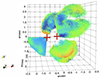 |
Fig. 20. Three-dimensional representation of the hot molecular outflow structures detected in Arp 220 modeled with MOKA3D. The XY represents the plane of the sky, while the Z axis is the LOS. The color intensity represents the intrinsic cloud emission, bluer colors represent lower emission clouds, while redder colors represent high-emission clouds. (See Marconcini et al. 2023 for the details of the model.) |
In all outflows, the velocities defined by Eq. (6) seem to underestimate the velocities found by the MOKA3D even though they are consistent within 1-2σ. This is due to the fact that the model takes into account the intrinsic velocity of the outflow corrected for all projection effects. In conclusion, the kinematic outflow properties inferred with MOKA3D and the method outlined in Sect. 5.3 are consistent within the uncertainties.
6. Discussion
The ubiquity of multiphase outflows in ULIRGs was established through spatially resolved observations in the visible band, thanks to integral field instruments like VIMOS and MUSE (Arribas et al. 2014; Westmoquette et al. 2012; Venturi et al. 2021; Musiimenta et al. 2024), in the near IR band with Gemini/NIFS, Keck/OSIRIS, and VLT/SINFONI (Engel et al. 2011; Riffel et al. 2015; Storchi-Bergmann et al. 2010; Pereira-Santaella et al. 2016; Emonts et al. 2017; U et al. 2019; Schönell et al. 2019), and in the radio band with ALMA (Pereira-Santaella et al. 2016).
Simulations show that outflows likely contain cold, dense clouds that are accelerated by a stream of warm and hot gas (e.g., Wagner et al. 2012; Zubovas & King 2014). However, the direct comparison of outflows identified with different tracers (and facilities), required to test such predictions, has been so far limited to very few targets. A key challenge in studying the direct impact of outflows on the ISM is the need for both high sensitivity and spatial resolution. Ground-based near-IR integral field facilities like SINFONI, OSIRIS and NIFS mainly traced the hot molecular (e.g., H2) and ionized (Brγ) gas with high spatial and spectral resolution. However, due to limitations in sensitivity and the presence of airglow emission lines, it has not always possible to fully characterize these outflows and compute directly their properties (e.g Riffel et al. 2014; Emonts et al. 2017; U et al. 2019; Bianchin et al. 2022). This is critical in order to characterize the connection between the warm molecular and the ionized gas outflow with the cold molecular gas. In fact, thanks to the advent of millimeter/submillimeter telescopes such as ALMA, high-spatial-resolution images of cold molecular gas in nearby galaxies have enabled us to reveal the structure and the morphology of starburst-driven and AGN-driven molecular outflows in high details (e.g Salak et al. 2020; Lamperti et al. 2022; Holden et al. 2024).
6.1. The multiphase outflows
Cold molecular outflows have been detected in the nuclear region of Arp 220 with different emission line tracers, such as HCO+, H2O, H2O+, OH, and OH+ (Sakamoto et al. 2009; González-Alfonso et al. 2012; Veilleux et al. 2013; Tunnard et al. 2015; Martín et al. 2016; Zschaechner et al. 2016). However, most of them are unresolved and therefore their morphology could not be constrained. Spatially resolved outflows studies have been conducted by Barcos-Muñoz et al. (2018) and Wheeler et al. (2020) with ALMA, and Perna et al. (2020) with MUSE. Thanks to the possibility of resolving multiphase outflows with NIRSpec, we can compare the outflow properties of hot molecular and ionized phases derived in this work, with those obtained from previous observations for cold molecular gas and ionized gas at larger scale. This will help us understand the connection between multiphase and multiscale outflows. After discussing the structures of these outflows, we examine the mechanisms responsible for launching them.
6.1.1. W nucleus-driven outflows
Barcos-Muñoz et al. (2018) reported a cold molecular outflow launched by the W nucleus, traced by HCN(1-0), extending for 120 pc, with a deprojected velocity of 850 km s−1 and a lower limit of the H2 mass for the redshifted and blueshifted component of ≳ 8 × 10⁶ M⊙ and ≳ 2 × 10⁶ M⊙, respectively. These lower limits consider the possible presence of additional outflowing material at lower velocities, not accounted due to its overlap with the disk emission. Wheeler et al. (2020) found an upper limit for the total H2 molecular mass of ≲ 2 × 10⁷ M⊙ for the redshifted outflow, and 2 × 10⁶ M⊙ for the blueshifted, traced by CO(3–2) gas. The upper limit here accounts the possible contamination of H13CN (4–3) emission, very close to the CO(3–2) transition.
We detected an HG-shape outflow originating from the W nucleus extending for 600 pc, with a hot H2 outflowing gas mass of 2000 M⊙. The redshifted region accounts for ∼1200 M⊙, while the blueshifted for ∼800 M⊙. This outflow is in the same direction as the cold molecular outflow detected in Wheeler et al. (2020), with receding gas northward and approaching gas southward. Therefore, we can reasonably assume that cold and hot molecular outflows are connected and associated with the same outflow event. Under this assumption, the total mass of the hot and cold molecular gas result in an estimated hot-to-cold molecular gas ratio of ≈10−4, obtained considering both receding and approaching gas. This order-of-magnitude estimate is consistent with the values 1 − 7 × 10⁻⁵ found in nearby ULIRGs (Pereira-Santaella et al. 2016; Emonts et al. 2017; Pereira-Santaella et al. 2018; Lamperti et al. 2022).
After comparing the total outflowing mass of ionized and total molecular gas in the W nucleus and hence accounting for both HGO and WNO, we report a mass outflow ratio between the two phases of 0.16 assuming [S II]-based electron densities (∼6 × 10⁻³ with the density estimated with [Fe II]). This is not unusual since the molecular phase usually dominates the mass outflow rate budget, exceeding the ionized gas phase by one to three orders of magnitude (Rupke & Veilleux 2013; García-Burillo et al. 2015; Carniani et al. 2015; Fiore et al. 2017; Cresci et al. 2023).
Perna et al. (2020) identified an extended structure associated with high-velocity ionized gas (see their Fig. 19, velocity channel 125 km s−1 < |v| < 375 km s−1) from northeast to southwest, that appears to be aligned with the hourglass-shaped outflow launched from the W nucleus. This suggests that the HGO could even be connected to the outflow detected at larger scales. Alternatively, they could trace different ejection events along the same direction.
6.1.2. E nucleus-driven outflows
Wheeler et al. (2020) reported a collimated and extended molecular outflow in the E nucleus traced by CO transitions (J = 3 → 2). The outflow found in the present work (SEO), launched from the E nucleus, is consistent with the direction of the outflow observed in the cold molecular gas, blueshifted toward the south direction. Wheeler et al. (2020) reported a mass for the blueshifted outflow of 2.7 × 10⁶ M⊙, which, under the assumption that the CO outflow is associated with the SE outflow detected in our data, would lead to a hot-to-cold molecular gas ratio of ∼3 × 10⁻⁴. This is compatible with the value we inferred in Sect. 6.1.1 for the outflow launched by the W nucleus.
We attributed the NW bubble to the E nucleus, since this structure could represent the counterpart of the blushifted outflow detected in the SE direction. However, unlike the HGO, in this case there is no clear blushifted and redshifted part of the outflow. This may be due to different gas ejection events, or to the fact that the redshifted part of the outflow is more obscured. Another possibility is that we included part of the redshifted outflow launched from the E nucleus in the HGO, since the two outflows may overlap, as we can see in Fig. 5c. From Fig. 20 we see that MOKA3D assigns a higher flux weight to the clouds of the HGO near the W nucleus. This suggests the possibility of contamination from the redshifted counterpart of the SEO.
We find that the mass of the ionized gas in the NW bubble, assuming ne = 170 cm−3, is ∼6 × 10⁵ M⊙, with a total energy of ∼2 × 1054 erg. Lockhart et al. (2015) estimated the properties of the NW bubble using Hα+[NII] narrow band imaging obtained with HST/WC3 with a resolution of 0.0396″/pixel, corresponding to 15 pc. They used assumptions different from ours on the density, on velocity of the bubble and also on the geometry. In fact, they adopted ne = 10 cm−3, about one order of magnitude lower than that used in this work, a velocity of 250 km s−1, around a factor 2 lower and a shell-like geometry. Despite these different assumptions, their derived outflow mass (3.2 × 10⁶ M⊙) and energy (2.0 × 1054 erg) are in agreement, within a factor of two, with our results.
We also compared the outflows detected with NIRSpec with the larger scale outflows observed with MUSE in Perna et al. (2020). In that case, the most extreme velocities for the ionized outflow are observed along PA = 138°;2 these extreme motions are aligned with X-ray emission and with the minor axis of the stellar disk. The SEO and the NWB are found along the same PA, but at < 1 kpc scales, which might suggest that they are related to the kiloparsec-scale atomic outflow presented in Perna et al. (2020). The ionized, large-scale bubble observed in MUSE (∼10 kpc) and the NW bubble could be, also in this case, the results of different outflow episodes. These multiple bubbles at different distances are very similar to those predicted by the TNG50 cosmological simulation as a result of AGN feedback (Nelson et al. 2019) and to those observed in NGC 1275 (e.g., Fabian et al. 2003; Sanders & Fabian 2007) and in the Tea Cup (Venturi et al. 2023).
6.2. The launching mechanism
The presence of AGN in the Arp 220 nuclei has been investigated in many previous works (e.g., Teng et al. 2015; Paggi et al. 2017; Yoast-Hull & Murray 2019; Perna et al. 2024), but conclusive evidence confirming their existence remains elusive. Furthermore, understanding whether outflows are powered by AGN or starburst presents an even greater challenge; in this section we relate the energetics of the Arp 220 multiphase outflows to the properties of AGN (if present) and SF, and we discuss possible scenarios.
To evaluate the effect of the outflows on the SF activity, we can compare their energetics with the SFR. However, the SFR varies depending on the band in which it is calculated, spanning values from 150 M⊙ yr−1 in the radio band (Varenius et al. 2016) to 0.5 M⊙ yr−1 through Paα (Perna et al. 2024) in the W nucleus, and from 80 to 0.17 M⊙ yr−1 in the E nucleus. Since the SFR measurements obtained from optical and near-IR features may be significantly affected by dust attenuation, leading to underestimation, we focus on the case where the SFR is calculated using the radio band.
Summing all the contributions of the outflows in the ionized and molecular phases in each nucleus, we derive a mass loading factor η of ∼0.13 and 0.15 and a Ėout of 1.1 × 1042 erg s−1 and 9 × 1041 erg s−1 for the W and E nuclei, respectively. We note that these values are only marginally affected by the densities used, since the main contribution comes from the cold molecular gas. These values are similar to those measured in other local ULIRGs (Arribas et al. 2014; Chisholm et al. 2017; Lamperti et al. 2022) and high-z star-forming galaxies (Genzel et al. 2014; Heckman et al. 2015; Newman et al. 2012; Perna et al. 2017, 2018). Moreover, they are in agreement with models where feedback from supernovae is the main outflow driver (e.g., Finlator & Davé 2008; Heckman et al. 2015).
Following Veilleux et al. (2005), we can derive the expected energy outflow rate by assuming proportionality with SFR (measured from radio band) and assuming solar metallicity. We derive ĖSFR = 1 × 1044 erg s−1 for the W nucleus and 6 × 1043 erg s−1for the E nucleus. Comparing these values expected for stellar activities with those obtained in previous paragraph, we find Ėout/ĖSFR of the order of a few percent, in agreement with a starburst-driven outflow expectations.
Paggi et al. (2017) estimated AGN luminosities in the 2 − 10 keV X-ray band of 0.5 × 1042 erg s−1 and 1.6 × 1042 erg s−1 for the W and E nuclei that lead to bolometric luminosities of 2.5 × 1043 erg s−1 and 8.3 × 1043 erg s−1, respectively. We also estimated the AGN luminosity from the total IR luminosity, assuming an AGN contribution of 6% to Lbol (Perna et al. 2021) and using the relative contribution of each nucleus measured in the ALMA continuum maps by Pereira-Santaella et al. (2021): Lbol = 2.5 × 1044 erg s−1 (W) and 1.1 × 1044 erg s−1 (E). It is worth noting that the AGN bolometric luminosity of the W nucleus inferred from FIR measurements is approximately 1 dex higher than the X-ray-based estimate, highlighting the challenges in constraining AGN activity in Arp 220. The outflow energetics computed in this section result in kinetic coupling efficiency values Ėout/LAGN = 0.005 − 0.05 for the W nucleus, and Ėout/LAGN = 0.009 − 0.01 for the W nucleus. These values are consistent with both theoretical predictions of kinetic coupling efficiencies in energy-conserving (∼0.005–0.05, e.g., Hopkins & Quataert 2010; Zubovas & King 2012; Costa et al. 2014; King & Pounds 2015) and radiation pressure-driven outflows (∼0.001–0.01, e.g., Costa et al. 2018; Ishibashi et al. 2018).
These results show that there are no arguments at present to prefer SF- to AGN-driven outflows, since both of the scenario are possible. We note, however, that the typical dynamical timescales tdyn = Rout/vout associated with the outflows in Arp 220 are approximately 1 Myr (see Table 3). In contrast, the SFR ≈ 100 M⊙ yr−1 used to compare outflow energetics with expectations for starburst-driven outflows reflects the SF history over a much longer period (up to 100 Myr; Kennicutt & Evans 2012). Following on these arguments, we consider two scenarios. In the former, we assume that the SFR in the past few million years is ≪100 M⊙ yr−1. This would be consistent with the SFR measured in the host from UV, optical and near-IR observations (e.g., Chandar et al. 2023; Perna et al. 2020, 2024; Giménez-Arteaga et al. 2022), as well as with the emission from supernovae and supernovae remnants at wavelengths from 2 to 18 cm which can be responsible for up to 20% of the total radio emission at GHz frequencies (but see the detailed discussion in Varenius et al. 2019). In this framework, the mass loading factors and outflow energetics would imply the presence of AGN winds, as SF would not provide enough energy to explain the outflow properties (η > 40, Ėout/ĖSFR > 3). In the second scenario, we assume the presence of extremely high attenuation at the position of the two nuclei, of AV > 100: such attenuation is required to match the SFR(PAH 3.3 μm) ∼ 1 M⊙ yr−1 with measurements from FIR and GHz frequencies. With this assumption, both starburst- and AGN-driven winds can be responsible for the observed outflows, according to the outflow energetics computed in this work.
In conclusion, further investigations are required to constrain the current SFR and the AGN activity in the nuclear regions of Arp 220. This information is essential for understanding the mechanisms driving the multiphase and multiscale outflows observed in this galaxy.
7. Conclusions
Using the exceptional JWST/NIRSpec facility, we investigated the complex multiphase structure and kinematics in the nuclear region of the ULIRG merging system Arp 220. We spatially resolved the emission of ionized gas (Paα) and hot molecular gas (H2 1-0 S(1) 2.12 μm) in the central kiloparsec of the nuclear region of Arp 220 in order to identify and disentangle several high-velocity multiphase outflows associated with the two nuclei of the system. We modeled the emission of the outflows with MOKA3D and inferred the intrinsic geometric and kinematic properties, finding agreement with the properties inferred from standard methods. We calculated the outflow mass and energetics of both ionized and hot molecular gas, and compared them with theoretical expectations for outflows driven by SF and AGN activity. In the following, we summarize our main findings.
-
We detected outflowing H2 and ionized gas with an hourglass shape launched by the W nucleus with an inclination of -60° with respect to the LOS as retrieved from MOKA3D and extending out to a distance of 600 pc with velocities of ∼500 km s−1. We also found an ionized compact outflow around the W nucleus, with velocities of up to 550 km s−1 and without a hot molecular gas counterpart.
-
We observed a hot molecular and ionized conical outflow in the southwest direction launched by the E nucleus with an inclination of 70° with respect to the LOS reaching velocities of up to 600 km s−1 and extending to the edges of the NIRSpec FoV (i.e., at least up to 400 pc). We also detected a multiphase blueshifted large-scale (∼1 kpc) bubble in northwest direction with an inclination of 68° with respect to the LOS and with velocities of up to 1100 km s−1. These high-velocity components are aligned with the larger-scale (∼10 kpc) outflow observed with MUSE, suggesting that they are part of the same outflow event originating from the E nucleus.
-
We combined NIRSpec and ALMA outcomes to infer a hot-to-cold molecular gas ratio of ∼10−4 for the outflows launched by the W and E nuclei, which is consistent with previous measurements for other ULIRGs from the literature. Considering the material launched by the E and W nuclei together, the largest contribution to the total outflow mass rate comes from cold molecular gas (∼20 M⊙ yr−1), followed by ionized gas (∼10 M⊙ yr−1, assuming [S II]-based ne) and hot molecular gas (∼0.003 M⊙ yr−1).
-
We discussed the possible origin of the outflows, and we conclude that there are no arguments at present to prefer SF- over AGN-driven outflows since both scenarios are possible. In particular, both recent nuclear activity with SFR ∼ 100 M⊙ yr−1 and AGN luminosity of ∼1043 − 1044 erg s−1 could explain the measured outflow mass loading factors (≈0.1), mass outflow rates (≈20 M⊙ yr−1), and kinetic powers (Ėout ≈ 1042 erg s−1), according to theoretical predictions.
The NIRSpec observations allowed us to connect the 100 pc scale cold molecular outflows revealed by ALMA (e.g., Wheeler et al. 2020) with the greater than 1 kpc scale ionized and neutral outflows identified in the MUSE data cube (e.g., Perna et al. 2020). These findings highlight the significant role that individual outflows launched by each nucleus during a merger could play in the starburst-quasar evolutionary sequence. These outflows propagate in multiple directions on kiloparsec scales, potentially impacting the overall physical and dynamical conditions of the ISM in the host galaxy and are at odds with the more compact, spherical outflows detected in other nearby systems (e.g., Venturi et al. 2021). Simulations predict that multidirectional outflows could lead to more uniform quenching of SF throughout the galaxy. In contrast, collimated outflows may be limited to specific directions and may allow SF to continue in other parts of the galaxy (see, e.g., Wagner et al. 2012; Nelson et al. 2019; Torrey et al. 2020; Sivasankaran et al. 2024).
We also investigated the properties of the ISM not participating in the outflow in terms of recent SF traced by recombination lines and obscuration. Additionally, we compared the stellar and the gas kinematics in both the close surroundings of the two nuclei and across the large-scale disk. The key findings of this analysis are summarized below.
-
Consistent with previous works, we found that SFR calculated with recombination lines (∼8 M⊙ yr−1) differs from the SF computed with FIR and radio (∼230 M⊙ yr−1). This result possibly indicates that a large fraction of the SF is completely obscured at near-IR wavelengths. Alternatively, the FIR measurements of SFR may trace SF on different timescales.
-
We estimated the attenuation from different emission line ratios: [Fe II] 1.644 μm/[Fe II] 1.257 μm, Brγ/Paβ, and Paα/Paβ. These values are consistent within 20%. The highest values are found at the position of the E nucleus, AV ∼ 10 mag, and the lowest values (AV ∼ 2 − 4 mag) are in the outer regions (∼400 pc distance from the nuclei).
-
The stellar and gas kinematics show a relatively good match, with the stellar component following the ionized gas rotation and appearing to rotate faster than the hot molecular gas.
The near-IR, spatially resolved spectroscopic data of Arp 220 presented in this work demonstrates the power of JWST/NIRSpec to disentangle the complex kinematics in the nuclear regions and to understand the interplay between multiphase outflows in the circumnuclear environments of nearby ULIRGs. Moreover, the data shed light on the feedback mechanisms in this peculiar phase of galaxy evolution.
Data availability
The data cube, the spectra shown in Fig. 2, and line maps presented in Fig. 4 are available at the CDS via anonymous ftp to cdsarc.cds.unistra.fr (130.79.128.5) or via https://cdsarc.cds.unistra.fr/viz-bin/cat/J/A+A/693/A36
The position angle is measured on the receding half of the galaxy, taken anticlockwise from the north direction on the sky (east of north).
Measured anti-clockwise from the north.
Acknowledgments
This article was produced while attending the PhD program in Space Science and Technology at the University of Trento, Cycle XXXVIII, with the support of a scholarship financed by the Ministerial Decree no. 351 of 9th April 2022, based on the NRRP – funded by the European Union – NextGenerationEU – Mission 4 “Education and Research”, Component 1 “Enhancement of the offer of educational services: from nurseries to universities” -Investment 4.1 “Extension of the number of research doctorates and innovative doctorates for public administration and cultural heritage” – E63C22001340001. MP, SA, and BRP acknowledge support from the research project PID2021-127718NB-I00 of the Spanish Ministry of Science and Innovation/State Agency of Research (MCIN/AEI/10.13039/501100011033). IL acknowledges support from PID2022-140483NB-C22 funded by AEI 10.13039/501100011033 and BDC 20221289 funded by MCIN by the Recovery, Transformation and Resilience Plan from the Spanish State, and by NextGenerationEU from the European Union through the Recovery and Resilience Facility. GC, AM acknowledge support from PRIN-MUR project “PROMETEUS” (202223XPZM), the INAF Large Grant 2022 “The metal circle: a new sharp view of the baryon cycle up to Cosmic Dawn with the latest generation IFU facilities” and INAF Large Grant 2022 “Dual and binary SMBH in the multi-messenger era”. KF acknowledges support through the ESA research fellowship programme. AJB acknowledges funding from the “FirstGalaxies” Advanced Grant from the European Research Council (ERC) under the European Union’s Horizon 2020 research and innovation program (Grant agreement No. 789056). FDE and RM acknowledge support by the Science and Technology Facilities Council (STFC), by the ERC through Advanced Grant 695671 “QUENCH”, and by the UKRI Frontier Research grant RISEandFALL. RM also acknowledges funding from a research professorship from the Royal Society. MPS acknowledges support from grants RYC2021-033094-I and CNS2023-145506 funded by MICIU/AEI/10.13039/501100011033 and the European Union NextGenerationEU/PRTR.
References
- Armus, L., Lai, T., U, V., et al. 2023, ApJ, 942, L37 [NASA ADS] [CrossRef] [Google Scholar]
- Arribas, S., Colina, L., & Clements, D. 2001, ApJ, 560, 160 [Google Scholar]
- Arribas, S., Colina, L., Alonso-Herrero, A., et al. 2012, A&A, 541, A20 [NASA ADS] [CrossRef] [EDP Sciences] [Google Scholar]
- Arribas, S., Colina, L., Bellocchi, E., Maiolino, R., & Villar-Martín, M. 2014, A&A, 568, A14 [NASA ADS] [CrossRef] [EDP Sciences] [Google Scholar]
- Barcos-Muñoz, L., Leroy, A. K., Evans, A. S., et al. 2015, ApJ, 799, 10 [Google Scholar]
- Barcos-Muñoz, L., Aalto, S., Thompson, T. A., et al. 2018, ApJ, 853, L28 [Google Scholar]
- Bautista, M. A., & Pradhan, A. K. 1998, ApJ, 492, 650 [NASA ADS] [CrossRef] [Google Scholar]
- Belfiore, F., Westfall, K. B., Schaefer, A., et al. 2019, AJ, 158, 160 [CrossRef] [Google Scholar]
- Bellocchi, E., Arribas, S., Colina, L., & Miralles-Caballero, D. 2013, A&A, 557, A59 [NASA ADS] [CrossRef] [EDP Sciences] [Google Scholar]
- Bellocchi, E., Pereira-Santaella, M., Colina, L., et al. 2022, A&A, 664, A60 [NASA ADS] [CrossRef] [EDP Sciences] [Google Scholar]
- Bennett, C. L., Larson, D., Weiland, J. L., & Hinshaw, G. 2014, ApJ, 794, 135 [Google Scholar]
- Bianchin, M., Riffel, R. A., Storchi-Bergmann, T., et al. 2022, MNRAS, 510, 639 [Google Scholar]
- Bohn, T., Inami, H., Togi, A., et al. 2024, arXiv e-prints [arXiv:2403.14751] [Google Scholar]
- Böker, T., Arribas, S., Lützgendorf, N., et al. 2022, A&A, 661, A82 [NASA ADS] [CrossRef] [EDP Sciences] [Google Scholar]
- Brusa, M., Feruglio, C., Cresci, G., et al. 2015, A&A, 578, A11 [NASA ADS] [CrossRef] [EDP Sciences] [Google Scholar]
- Calzetti, D., Armus, L., Bohlin, R. C., et al. 2000, ApJ, 533, 682 [NASA ADS] [CrossRef] [Google Scholar]
- Cappellari, M. 2017, MNRAS, 466, 798 [Google Scholar]
- Cappellari, M., & Copin, Y. 2003, MNRAS, 342, 345 [Google Scholar]
- Cappellari, M., & Emsellem, E. 2004, PASP, 116, 138 [Google Scholar]
- Cappellari, M., Emsellem, E., Bacon, R., et al. 2007, MNRAS, 379, 418 [Google Scholar]
- Cappellari, M., Neumayer, N., Reunanen, J., et al. 2009, MNRAS, 394, 660 [NASA ADS] [CrossRef] [Google Scholar]
- Carniani, S., Marconi, A., Maiolino, R., et al. 2015, A&A, 580, A102 [NASA ADS] [CrossRef] [EDP Sciences] [Google Scholar]
- Cazzoli, S., Arribas, S., Maiolino, R., & Colina, L. 2016, A&A, 590, A125 [NASA ADS] [CrossRef] [EDP Sciences] [Google Scholar]
- Chandar, R., Caputo, M., Linden, S., et al. 2023, ApJ, 943, 142 [NASA ADS] [CrossRef] [Google Scholar]
- Chisholm, J., Tremonti, C. A., Leitherer, C., & Chen, Y. 2017, MNRAS, 469, 4831 [NASA ADS] [CrossRef] [Google Scholar]
- Colina, L., Arribas, S., & Clements, D. 2004, ApJ, 602, 181 [Google Scholar]
- Costa, T., Sijacki, D., & Haehnelt, M. G. 2014, MNRAS, 444, 2355 [Google Scholar]
- Costa, T., Rosdahl, J., Sijacki, D., & Haehnelt, M. G. 2018, MNRAS, 479, 2079 [Google Scholar]
- Cresci, G., Tozzi, G., Perna, M., et al. 2023, A&A, 672, A128 [NASA ADS] [CrossRef] [EDP Sciences] [Google Scholar]
- Crespo Gómez, A., Piqueras López, J., Arribas, S., et al. 2021, A&A, 650, A149 [NASA ADS] [CrossRef] [EDP Sciences] [Google Scholar]
- Davis, C. J., Cervantes, B., Nisini, B., et al. 2011, A&A, 528, A3 [NASA ADS] [CrossRef] [EDP Sciences] [Google Scholar]
- D’Eugenio, F., Perez-Gonzalez, P., Maiolino, R., et al. 2023, arXiv e-prints [arXiv:2308.06317] [Google Scholar]
- Di Matteo, T., Springel, V., & Hernquist, L. 2005, Nature, 433, 604 [NASA ADS] [CrossRef] [Google Scholar]
- Domínguez, A., Siana, B., Henry, A. L., et al. 2013, ApJ, 763, 145 [CrossRef] [Google Scholar]
- Emonts, B. H. C., Colina, L., Piqueras-López, J., et al. 2017, A&A, 607, A116 [NASA ADS] [CrossRef] [EDP Sciences] [Google Scholar]
- Engel, H., Davies, R. I., Genzel, R., et al. 2011, ApJ, 729, 58 [NASA ADS] [CrossRef] [Google Scholar]
- Fabian, A. C., Sanders, J. S., Crawford, C. S., et al. 2003, MNRAS, 344, L48 [NASA ADS] [CrossRef] [Google Scholar]
- Ferland, G. J., Chatzikos, M., Guzmán, F., et al. 2017, Rev. Mex. A&A, 53, 385 [Google Scholar]
- Feruglio, C., Fiore, F., Carniani, S., et al. 2015, A&A, 583, A99 [NASA ADS] [CrossRef] [EDP Sciences] [Google Scholar]
- Finlator, K., & Davé, R. 2008, MNRAS, 385, 2181 [NASA ADS] [CrossRef] [Google Scholar]
- Fiore, F., Feruglio, C., Shankar, F., et al. 2017, A&A, 601, A143 [NASA ADS] [CrossRef] [EDP Sciences] [Google Scholar]
- Fluetsch, A., Maiolino, R., Carniani, S., et al. 2021, MNRAS, 505, 5753 [NASA ADS] [CrossRef] [Google Scholar]
- Förster Schreiber, N. M., Übler, H., Davies, R. L., et al. 2019, ApJ, 875, 21 [Google Scholar]
- García-Burillo, S., Combes, F., Usero, A., et al. 2015, A&A, 580, A35 [Google Scholar]
- Genzel, R., Newman, S., Jones, T., et al. 2011, ApJ, 733, 101 [Google Scholar]
- Genzel, R., Förster Schreiber, N. M., Rosario, D., et al. 2014, arXiv e-prints [arXiv:1406.0183] [Google Scholar]
- Giménez-Arteaga, C., Brammer, G. B., Marchesini, D., et al. 2022, ApJS, 263, 17 [CrossRef] [Google Scholar]
- González-Alfonso, E., Fischer, J., Graciá-Carpio, J., et al. 2012, A&A, 541, A4 [NASA ADS] [CrossRef] [EDP Sciences] [Google Scholar]
- Gustafsson, B., Edvardsson, B., Eriksson, K., et al. 2008, A&A, 486, 951 [NASA ADS] [CrossRef] [EDP Sciences] [Google Scholar]
- Heckman, T. M., Alexandroff, R. M., Borthakur, S., Overzier, R., & Leitherer, C. 2015, ApJ, 809, 147 [Google Scholar]
- Holden, L. R., Tadhunter, C., Audibert, A., et al. 2024, MNRAS, 530, 446 [NASA ADS] [CrossRef] [Google Scholar]
- Hopkins, P. F., & Quataert, E. 2010, MNRAS, 407, 1529 [Google Scholar]
- Hopkins, P. F., Hernquist, L., Cox, T. J., & Kereš, D. 2008, ApJS, 175, 356 [Google Scholar]
- Hummer, D. G., & Storey, P. J. 1987, MNRAS, 224, 801 [NASA ADS] [CrossRef] [Google Scholar]
- Hung, C.-L., Sanders, D. B., Casey, C. M., et al. 2014, ApJ, 791, 63 [NASA ADS] [CrossRef] [Google Scholar]
- Ishibashi, W., Fabian, A. C., & Maiolino, R. 2018, MNRAS, 476, 512 [NASA ADS] [Google Scholar]
- Isobe, Y., Ouchi, M., Nakajima, K., et al. 2023, ApJ, 956, 139 [NASA ADS] [CrossRef] [Google Scholar]
- Jakobsen, P., Ferruit, P., de Oliveira, C. A., et al. 2022, A&A, 661, A80 [NASA ADS] [CrossRef] [EDP Sciences] [Google Scholar]
- Kakkad, D., Mainieri, V., Vietri, G., et al. 2020, A&A, 642, A147 [NASA ADS] [CrossRef] [EDP Sciences] [Google Scholar]
- Kennicutt, R. C., & Evans, N. J. 2012, ARA&A, 50, 531 [NASA ADS] [CrossRef] [Google Scholar]
- King, A., & Pounds, K. 2015, ARA&A, 53, 115 [NASA ADS] [CrossRef] [Google Scholar]
- Koo, B.-C., Raymond, J. C., & Kim, H.-J. 2016, JKAS, 49, 109 [NASA ADS] [Google Scholar]
- Krajnović, D., Emsellem, E., Cappellari, M., et al. 2011, MNRAS, 414, 2923 [Google Scholar]
- Kristensen, L. E., Godard, B., Guillard, P., Gusdorf, A., & Pineau des Forêts, G. 2023, A&A, 675, A86 [NASA ADS] [CrossRef] [EDP Sciences] [Google Scholar]
- Lai, T. S. Y., Armus, L., U, V., et al. 2022, ApJ, 941, L36 [NASA ADS] [CrossRef] [Google Scholar]
- Lamperti, I., Pereira-Santaella, M., Perna, M., et al. 2022, A&A, 668, A45 [NASA ADS] [CrossRef] [EDP Sciences] [Google Scholar]
- Law, D. D., Morrison, J. E., Argyriou, I., et al. 2023, AJ, 166, 45 [NASA ADS] [CrossRef] [Google Scholar]
- Lockhart, K. E., Kewley, L. J., Lu, J. R., et al. 2015, ApJ, 810, 149 [CrossRef] [Google Scholar]
- Lonsdale, C. J., Farrah, D., & Smith, H. E. 2006, in Astrophysics Update 2, ed. J. W. Mason, 285 [CrossRef] [Google Scholar]
- Lucatelli, G., Beswick, R. J., Moldón, J., et al. 2024, MNRAS, 529, 4468 [NASA ADS] [CrossRef] [Google Scholar]
- Lutz, D., Sturm, E., Janssen, A., et al. 2020, A&A, 633, A134 [NASA ADS] [CrossRef] [EDP Sciences] [Google Scholar]
- Madau, P., & Dickinson, M. 2014, ARA&A, 52, 415 [Google Scholar]
- Marasco, A., Cresci, G., Nardini, E., et al. 2020, A&A, 644, A15 [EDP Sciences] [Google Scholar]
- Marconcini, C., Marconi, A., Cresci, G., et al. 2023, A&A, 677, A58 [NASA ADS] [CrossRef] [EDP Sciences] [Google Scholar]
- Martín, S., Aalto, S., Sakamoto, K., et al. 2016, A&A, 590, A25 [NASA ADS] [CrossRef] [EDP Sciences] [Google Scholar]
- May, D., & Steiner, J. E. 2017, MNRAS, 469, 994 [NASA ADS] [CrossRef] [Google Scholar]
- Mazzalay, X., Saglia, R. P., Erwin, P., et al. 2013, MNRAS, 428, 2389 [NASA ADS] [CrossRef] [Google Scholar]
- McDowell, J. C., Clements, D. L., Lamb, S. A., et al. 2003, ApJ, 591, 154 [NASA ADS] [CrossRef] [Google Scholar]
- McKinney, J., Pope, A., Kirkpatrick, A., et al. 2023, ApJ, 955, 136 [NASA ADS] [CrossRef] [Google Scholar]
- Musiimenta, B., Speranza, G., Urrutia, T., et al. 2024, A&A, 687, A111 [NASA ADS] [CrossRef] [EDP Sciences] [Google Scholar]
- Nardini, E., Risaliti, G., Watabe, Y., Salvati, M., & Sani, E. 2010, MNRAS, 405, 2505 [NASA ADS] [Google Scholar]
- Nelson, D., Springel, V., Pillepich, A., et al. 2019, Comput. Astrophys. Cosmol., 6, 29 [CrossRef] [Google Scholar]
- Newman, S. F., Genzel, R., Förster-Schreiber, N. M., et al. 2012, ApJ, 761, 43 [Google Scholar]
- Paggi, A., Fabbiano, G., Risaliti, G., et al. 2017, ApJ, 841, 44 [NASA ADS] [CrossRef] [Google Scholar]
- Pereira-Santaella, M., Colina, L., García-Burillo, S., et al. 2016, A&A, 594, A81 [NASA ADS] [CrossRef] [EDP Sciences] [Google Scholar]
- Pereira-Santaella, M., Colina, L., García-Burillo, S., et al. 2018, A&A, 616, A171 [NASA ADS] [CrossRef] [EDP Sciences] [Google Scholar]
- Pereira-Santaella, M., Colina, L., García-Burillo, S., et al. 2021, A&A, 651, A42 [NASA ADS] [CrossRef] [EDP Sciences] [Google Scholar]
- Perna, M., Lanzuisi, G., Brusa, M., Cresci, G., & Mignoli, M. 2017, A&A, 606, A96 [NASA ADS] [CrossRef] [EDP Sciences] [Google Scholar]
- Perna, M., Sargent, M. T., Brusa, M., et al. 2018, A&A, 619, A90 [NASA ADS] [CrossRef] [EDP Sciences] [Google Scholar]
- Perna, M., Arribas, S., Catalán-Torrecilla, C., et al. 2020, A&A, 643, A139 [NASA ADS] [CrossRef] [EDP Sciences] [Google Scholar]
- Perna, M., Arribas, S., Pereira Santaella, M., et al. 2021, A&A, 646, A101 [EDP Sciences] [Google Scholar]
- Perna, M., Arribas, S., Marshall, M., et al. 2023, A&A, 679, A89 [NASA ADS] [CrossRef] [EDP Sciences] [Google Scholar]
- Perna, M., Arribas, S., Lamperti, I., et al. 2024, A&A, 690, A171 [NASA ADS] [CrossRef] [EDP Sciences] [Google Scholar]
- Perrotta, S., Hamann, F., Zakamska, N. L., et al. 2019, MNRAS, 488, 4126 [Google Scholar]
- Piqueras López, J., Colina, L., Arribas, S., Alonso-Herrero, A., & Bedregal, A. G. 2012, A&A, 546, A64 [NASA ADS] [CrossRef] [EDP Sciences] [Google Scholar]
- Reddy, N. A., Topping, M. W., Sanders, R. L., Shapley, A. E., & Brammer, G. 2023, ApJ, 948, 83 [NASA ADS] [CrossRef] [Google Scholar]
- Revalski, M., Crenshaw, D. M., Rafelski, M., et al. 2022, ApJ, 930, 14 [NASA ADS] [CrossRef] [Google Scholar]
- Riffel, R. A., Storchi-Bergmann, T., & Riffel, R. 2014, ApJ, 780, L24 [Google Scholar]
- Riffel, R. A., Storchi-Bergmann, T., & Riffel, R. 2015, MNRAS, 451, 3587 [Google Scholar]
- Rupke, D. S. N., & Veilleux, S. 2013, ApJ, 768, 75 [Google Scholar]
- Sakamoto, K., Scoville, N. Z., Yun, M. S., et al. 1999, ApJ, 514, 68 [NASA ADS] [CrossRef] [Google Scholar]
- Sakamoto, K., Aalto, S., Wilner, D. J., et al. 2009, ApJ, 700, L104 [Google Scholar]
- Salak, D., Nakai, N., Sorai, K., & Miyamoto, Y. 2020, ApJ, 901, 151 [NASA ADS] [CrossRef] [Google Scholar]
- Sanders, J. S., & Fabian, A. C. 2007, MNRAS, 381, 1381 [Google Scholar]
- Sanders, D. B., & Mirabel, I. F. 1996, ARA&A, 34, 749 [Google Scholar]
- Sanders, D. B., Soifer, B. T., Elias, J. H., et al. 1988, ApJ, 325, 74 [Google Scholar]
- Schönell, A. J., Storchi-Bergmann, T., Riffel, R. A., et al. 2019, MNRAS, 485, 2054 [CrossRef] [Google Scholar]
- Scoville, N. Z., Hall, D. N. B., Ridgway, S. T., & Kleinmann, S. G. 1982, ApJ, 253, 136 [NASA ADS] [CrossRef] [Google Scholar]
- Scoville, N., Aussel, H., Brusa, M., et al. 2007, ApJS, 172, 1 [Google Scholar]
- Scoville, N., Murchikova, L., Walter, F., et al. 2017, ApJ, 836, 66 [Google Scholar]
- Silk, J. 2013, ApJ, 772, 112 [Google Scholar]
- Sivasankaran, A., Blecha, L., Torrey, P., et al. 2024, arXiv e-prints [arXiv:2402.15240] [Google Scholar]
- Soifer, B. T., Rowan-Robinson, M., Houck, J. R., et al. 1984, ApJ, 278, L71 [NASA ADS] [CrossRef] [Google Scholar]
- Storchi-Bergmann, T., Lopes, R. D. S., McGregor, P. J., et al. 2010, MNRAS, 402, 819 [NASA ADS] [CrossRef] [Google Scholar]
- Sturm, E., González-Alfonso, E., Veilleux, S., et al. 2011, ApJ, 733, L16 [NASA ADS] [CrossRef] [Google Scholar]
- Talia, M., Brusa, M., Cimatti, A., et al. 2017, MNRAS, 471, 4527 [NASA ADS] [CrossRef] [Google Scholar]
- Teng, S. H., Rigby, J. R., Stern, D., et al. 2015, ApJ, 814, 56 [Google Scholar]
- Torrey, P., Hopkins, P. F., Faucher-Giguère, C.-A., et al. 2020, MNRAS, 497, 5292 [NASA ADS] [CrossRef] [Google Scholar]
- Tozzi, G., Cresci, G., Marasco, A., et al. 2021, A&A, 648, A99 [NASA ADS] [CrossRef] [EDP Sciences] [Google Scholar]
- Tunnard, R., Greve, T. R., Garcia-Burillo, S., et al. 2015, ApJ, 800, 25 [NASA ADS] [CrossRef] [Google Scholar]
- U, V., Sanders, D. B., Mazzarella, J. M., et al. 2012, ApJS, 203, 9 [Google Scholar]
- U, V., Medling, A. M., Inami, H., et al. 2019, ApJ, 871, 166 [Google Scholar]
- Ueda, J., Michiyama, T., Iono, D., Miyamoto, Y., & Saito, T. 2022, PASJ, 74, 407 [NASA ADS] [CrossRef] [Google Scholar]
- Varenius, E., Conway, J. E., Martí-Vidal, I., et al. 2016, A&A, 593, A86 [NASA ADS] [CrossRef] [EDP Sciences] [Google Scholar]
- Varenius, E., Conway, J. E., Batejat, F., et al. 2019, A&A, 623, A173 [NASA ADS] [CrossRef] [EDP Sciences] [Google Scholar]
- Veilleux, S., Cecil, G., & Bland-Hawthorn, J. 2005, ARA&A, 43, 769 [NASA ADS] [CrossRef] [Google Scholar]
- Veilleux, S., Meléndez, M., Sturm, E., et al. 2013, ApJ, 776, 27 [Google Scholar]
- Venturi, G., Cresci, G., Marconi, A., et al. 2021, A&A, 648, A17 [NASA ADS] [CrossRef] [EDP Sciences] [Google Scholar]
- Venturi, G., Treister, E., Finlez, C., et al. 2023, A&A, 678, A127 [NASA ADS] [CrossRef] [EDP Sciences] [Google Scholar]
- Villar Martín, M., Emonts, B., Humphrey, A., Cabrera Lavers, A., & Binette, L. 2014, MNRAS, 440, 3202 [CrossRef] [Google Scholar]
- Wagner, A. Y., Bicknell, G. V., & Umemura, M. 2012, ApJ, 757, 136 [CrossRef] [Google Scholar]
- Westmoquette, M. S., Clements, D. L., Bendo, G. J., & Khan, S. A. 2012, MNRAS, 424, 416 [NASA ADS] [CrossRef] [Google Scholar]
- Wheeler, J., Glenn, J., Rangwala, N., & Fyhrie, A. 2020, ApJ, 896, 43 [NASA ADS] [CrossRef] [Google Scholar]
- Yoast-Hull, T. M., & Murray, N. 2019, MNRAS, 484, 3665 [NASA ADS] [CrossRef] [Google Scholar]
- Zschaechner, L. K., Ott, J., Walter, F., et al. 2016, ApJ, 833, 41 [CrossRef] [Google Scholar]
- Zubovas, K., & King, A. 2012, ApJ, 745, L34 [Google Scholar]
- Zubovas, K., & King, A. R. 2014, MNRAS, 439, 400 [Google Scholar]
Appendix A: G140H stellar kinematics
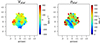 |
Fig. A.1. Stellar kinematics derived from the analysis of the first cube (grating G140H/F100LP). |
Appendix B: MOKA3D
In the Appendix B, we show the comparison of the data and the kinematic model MOKA3D for the SE outflow, HG outflow and NW bubble as discussed in Sect. 5.4.
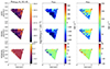 |
Fig. B.1. Comparison between the flux and velocity of H2 (top panels) and MOKA3D weighted model (middle panels) for the SE conical outflow. The bottom panels present the residuals obtained subtracting the model from the data. |
All Tables
Coordinates and systemic redshift of the two nuclei of Arp 220 from Perna et al. (2024).
All Figures
|
Fig. 1. Three-color emission line images of Arp 220. The emission line maps are obtained integrating the continuum-subtracted data-cube around [Fe II] 1.257 μm (left), Paα (center), and H2 1–0 S(1) 2.122 μm (right) in the velocity ranges −400 km s−1 < v < −200 km s−1 (blue), −200 km s−1 < v < 200 km s−1 (green) and 200 km s−1 < v < 400 km s−1 (red), with respect to the median value between zE* and zW*, zm = 0.0181. The red crosses mark the position of the two nuclei. |
| In the text | |
|
Fig. 2. Arp 220 W and E nuclear spectra. The spectra were extracted from a circular aperture of radius 3 spaxels (corresponding to 0.15″) and are reported in units of flux density as a function of rest-frame wavelength. Red dashed vertical lines identify H2 lines; black dashed lines identify ionized gas transitions. Gold-filled areas mark the position of the main CO stellar absorption lines. |
| In the text | |
|
Fig. 3. Arp 220 W and E nuclear spectra with pPXF best-fit models. The CO absorption features are in the 1.5–1.7 μm band (upper panel) and 2.2–2.36 μm (bottom panel). Black and green curves respectively refer to the data and the model of the W nucleus spectrum. Brown and gold curves respectively refer to the data and the model of the E nucleus spectrum. Black dashed vertical lines indicate the position of the main CO absorption lines. |
| In the text | |
|
Fig. 4. Moment maps of hot molecular gas (H2 1-0S(1), top) and ionized gas (center: Paα, bottom: [Fe II] 1.257 μm). The moment-1 was computed with respect to zm = 0.0181. An S/N cut of three on the flux of each emission line was applied to the maps. The black “+” symbols mark the position of the E and W nuclei. White contours represent the edges of the masks described in Sect. 4. |
| In the text | |
|
Fig. 5. Arp 220 outflow regions. (a): Composite view of the isolated outflow regions: southeast outflow (red), hour-glass outflow (blue), northwest outflow (green). (b): Channel map between −650 and −300 km s−1 in the H2 transition with respect to the systemic redshift of the E nucleus. The white curve indicates the edges of the SEO mask. (c): Sum of channel maps < − 200 and > 200 km s−1 in the H2 transition with respect to the systemic redshift of the W nucleus. The white curve indicates the edges of the HG region. (d): Sum of H2 and Paα channel maps between −800 and −450 km s−1 with respect to the systemic redshift of the E nucleus. The white curve indicates the edges of the NWB region. |
| In the text | |
|
Fig. 6. SE conical outflow flux and velocity maps. From left to right: flux of H2 and Paα lines, velocity, and velocity of the Gaussian component attributed to the SE outflow. The velocities are relative to the systemic velocity of the E nucleus. Red crosses indicate the positions of the two nuclei. Green asterisks in the first panel indicate the spaxels presented in Fig. 7. |
| In the text | |
|
Fig. 7. Spectra extracted from the SE outflow cone. The solid black curves represent the line profiles of H2 (top) and Paα (bottom) extracted from the spaxel close to the E nucleus (A), in the central part of the cone (B), and at the edge of the collimated outflow (C), as labeled in Fig. 6. The multi-Gaussian fits are depicted by dashed orange curves for the disk components and solid red curves for the outflow component. The total model for the disk is shown as a solid orange curve, and the combined model for both disk and outflow is displayed in green. The blue dots indicate the residuals. The velocities are computed with respect to the systemic velocity of the E nucleus. |
| In the text | |
|
Fig. 8. HG outflow flux and velocity maps. From left to right: flux of H2 and Paα lines, velocity, and velocity dispersion of the Gaussian component attributed to the HG outflow. The velocities are relative to the systemic velocity of the W nucleus. Red crosses indicate the positions of the two nuclei. Green asterisks in the first panel indicate the spaxels presented in Fig. 9. |
| In the text | |
|
Fig. 9. Spectra extracted from the HG outflow region. The solid black curves represent the line profiles of H2 (top) and Paα (bottom) extracted from the spaxels marked in Fig. 8. The red curve refers to the HG outflow. Orange curves identify the additional components used for the fit (orange dashed curves). The combined model is displayed in green. The velocities are computed with respect to the systemic velocity of the W nucleus. |
| In the text | |
|
Fig. 10. NW bubble flux and velocity maps. From left to right: flux of H2 and Paα lines, velocity, and velocity dispersion of the Gaussian component attributed to the outflow. The velocity is referred to the E nucleus. Red crosses indicate the positions of the two nuclei. Green asterisks in the first panel indicate the spaxels presented in Fig. 11. |
| In the text | |
|
Fig. 11. Spectra extracted from the NW bubble region. Line profiles of H2 (top) and Paα (bottom) are shown at the position of the three spaxels labeled in Fig. 10. The black dashed curves represent the spectra from the original cube, highlighting the contribution attributed to the HGO (red-shaded area) that we have already isolated and subtracted; the black solid lines represent the spectra fitted to identify the NW bubble. The red Gaussian profiles identify the isolated NW bubble, while orange profiles identify the rotating disk component. The combined model is displayed in green. The velocities are computed with respect to the systemic velocity of the E nucleus. |
| In the text | |
|
Fig. 12. Moment maps of the large-scale rotating disk and the W nuclear outflow. Top and middle panels: moment-0 (left), moment-1 (center), and moment-2 (right) maps of H21-0S(1) (top) and Paα (middle) of the Gaussian components attributed to the perturbed disk. The black-dashed line in the velocity maps show the large-scale disc mean kinematic major-axis (PA = 45°). Bottom panels: Paα moments maps of the Gaussian components attributed to the W nuclear outflow. Velocities are referred to zm in the first two rows. Velocity in the zoom-in inset is referred to the systemic velocity of the W nucleus. |
| In the text | |
|
Fig. 13. Spectrum extracted from the WNO. Line profiles of H2 (left) and Paα (right) extracted from a spaxel labeled in the bottom panel of Fig. 12). The two component fits are represented by the dashed orange (disc component) and red (outflow component) curves; the combined model is displayed in green. The velocities are computed with respect to the systemic velocity of the W nucleus. |
| In the text | |
|
Fig. 14. Spectra extracted from the kiloparsec-scale disk. Line profiles of H2 (top) and Paα (bottom) at the position of the three spaxels labeled in Fig. 12. The black dashed curves represent the spectra from the original cube, highlighting the contribution attributed to the HGO and SEO (red-shaded area) that we have already isolated and subtracted; the black solid lines represent the spectra fitted to identify the large-scale disk. The red dashed curves show the components associated with the disk model. The total disk model is shown with a solid red curve. Velocities are computed with respect to zm. |
| In the text | |
|
Fig. 15. Stellar kinematics maps. Top panels: Stellar velocity (left, in the frame zm) and velocity dispersion (right). Bottom panels: Stellar velocity (left) and velocity dispersion (right) around the two nuclei shifted with respect to the rest-frame velocity of each nucleus. Black dashed lines refer to the major axis of the two nuclei (W: PA = 257°, E: PA = 45°). Light blue dashed line refers to the axis of HG outflow (PA = 13°). |
| In the text | |
|
Fig. 16. Position-velocity diagram for ionized gas (top) and hot molecular gas (bottom) of W nucleus with positions varying along the disk major axis (PA = 257°, left, with positive distances toward west), the disk minor axis (PA = 347°, center, with positive distances toward north); and HG outflow axis (PA = 13°, right, with positive distances toward southwest). Black stars represent the stellar velocity. The zero-velocity refers to |
| In the text | |
|
Fig. 17. Position-velocity diagrams of large-scale rotational disk centered on the E nucleus. In the left panels, the positions vary along the mean kinematic major axis (PA = 45°), with positive distances toward south-west. In the right panels, the positions vary along the minor axis (PA = 135°), with positive distances toward north-west. The upper panels show the PV diagrams of Paα, while the lower panels show PV diagrams of H2 1-0 S(1). Black stars identify the stellar kinematics. The zero-velocity refers to |
| In the text | |
|
Fig. 18. Dust attenuation maps from the[Fe II] 1.257 μm to [Fe II] 1.640 μm ratio (left), Brγ/Paβ (middle) and Paα/Paβ (right). |
| In the text | |
|
Fig. 19. Maps of ionized over hot molecular gas ratio and SF surface density. (a) Spatially resolved flux ratio log(Paα/H2) computed from the total profile of the two lines. (b): Surface density map of the SFR inferred from Paα after subtraction of the outflowing components. |
| In the text | |
|
Fig. 20. Three-dimensional representation of the hot molecular outflow structures detected in Arp 220 modeled with MOKA3D. The XY represents the plane of the sky, while the Z axis is the LOS. The color intensity represents the intrinsic cloud emission, bluer colors represent lower emission clouds, while redder colors represent high-emission clouds. (See Marconcini et al. 2023 for the details of the model.) |
| In the text | |
|
Fig. A.1. Stellar kinematics derived from the analysis of the first cube (grating G140H/F100LP). |
| In the text | |
|
Fig. B.1. Comparison between the flux and velocity of H2 (top panels) and MOKA3D weighted model (middle panels) for the SE conical outflow. The bottom panels present the residuals obtained subtracting the model from the data. |
| In the text | |
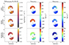 |
Fig. B.2. Same as B.1 for the HG outflow. |
| In the text | |
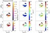 |
Fig. B.3. Same as B.1 for the NW bubble. |
| In the text | |
Current usage metrics show cumulative count of Article Views (full-text article views including HTML views, PDF and ePub downloads, according to the available data) and Abstracts Views on Vision4Press platform.
Data correspond to usage on the plateform after 2015. The current usage metrics is available 48-96 hours after online publication and is updated daily on week days.
Initial download of the metrics may take a while.