| Issue |
A&A
Volume 691, November 2024
|
|
|---|---|---|
| Article Number | A300 | |
| Number of page(s) | 17 | |
| Section | Cosmology (including clusters of galaxies) | |
| DOI | https://doi.org/10.1051/0004-6361/202451064 | |
| Published online | 20 November 2024 | |
XMM-SERVS X-ray extended Galaxy Cluster (XVXGC) catalog
1
Kavli Institute for Astronomy and Astrophysics (KIAA), Peking University,
Beijing
100871,
China
2
National Astronomical Observatories (NAOC), Chinese Academy of Sciences,
Beijing
100101,
China
3
Institute for Frontiers in Astronomy and Astrophysics, Beijing Normal University,
Beijing
102206,
China
4
Department of Astronomy, School of Physics, Peking University,
Beijing
100871,
China
5
School of Astronomy and Space Science, University of Chinese Academy of Science,
Beijing
100049,
China
6
School of Astronomy and Space Science, Nanjing University,
Nanjing,
Jiangsu
210093,
China
7
Key Laboratory of Modern Astronomy and Astrophysics (Nanjing University), Ministry of Education,
Nanjing,
Jiangsu
210093,
China
8
Department of Astronomy and Astrophysics,
525 Davey Lab, The Pennsylvania State University,
University Park,
PA
16802,
USA
9
Institute for Gravitation and the Cosmos, The Pennsylvania State University,
University Park,
PA
16802,
USA
10
Department of Physics, 104 Davey Lab, The Pennsylvania State University,
University Park,
PA
16802,
USA
11
College of Computer Science and Artificial Intelligence, Wenzhou University,
325035
Wenzhou,
China
12
Argelander-Institut für Astronomie (AIfA), Universität Bonn,
Auf dem Hügel 71,
53121
Bonn,
Germany
★ Corresponding author; This email address is being protected from spambots. You need JavaScript enabled to view it.
Received:
11
June
2024
Accepted:
18
September
2024
Abstract
Context. To explain the well-known tension between cosmological parameter constraints obtained from the primary cosmic microwave background (CMB) and those drawn from X-ray-selected galaxy cluster samples identified with early data, we propose a possible explanation for the incompleteness of detected clusters being higher than estimated. Specifically, we suggest that certain types of galaxy groups or clusters may have been overlooked in previous works.
Aims. We aim to search for galaxy groups and clusters with especially extended surface brightness distributions by creating a new X-ray-selected catalog of extended galaxy clusters from the XMM-Spitzer Extragalactic Representative Volume Survey (XMM-SERVS) data, based on a dedicated source detection and characterization algorithm optimized for extended sources.
Methods. Our state-of-the-art algorithm is composed of wavelet filtering, source detection, and characterization. We carried out a visual inspection of the optical image, and spatial distribution of galaxies within the same redshift layer to confirm the existence of clusters and estimated the cluster redshift with the spectroscopic and photometric redshifts of galaxies. The growth curve analysis was used to characterize the detections.
Results. We present a catalog of extended X-ray galaxy clusters detected from the XMM-SERVS data. The XMM-SERVS X-ray eXtended Galaxy Cluster (XVXGC) catalog features 141 cluster candidates. Specifically, there are 53 clusters previously identified as clusters with intracluster medium (ICM) emission (class 3); 40 that were previously known as optical or infrared (IR) clusters, but detected as X-ray clusters for the first time (class 2); and 48 identified as clusters for the first time (class 1). Compared with the class 3 sample, the “class 1 + class 2” sample is systematically fainter and exhibits a flatter surface brightness profile. Specifically, the median flux in [0.5–2.0] keV band for “class 1 + class 2” and class 3 sample is 1.288 × 10⁻¹⁴ erg/s/cm2 and 1.887 × 10⁻¹⁴ erg/s/cm2, respectively. The median values of β (i.e., the slope of the cluster surface brightness profile) are 0.506 and 0.573 for the “class 1 + class 2” and class 3 samples, respectively. The entire sample is available at the CDS.
Key words: catalogs / surveys / X-rays: galaxies: clusters
© The Authors 2024
 Open Access article, published by EDP Sciences, under the terms of the Creative Commons Attribution License (https://creativecommons.org/licenses/by/4.0), which permits unrestricted use, distribution, and reproduction in any medium, provided the original work is properly cited.
This article is published in open access under the Subscribe to Open model. This email address is being protected from spambots. You need JavaScript enabled to view it. to support open access publication.
1 Introduction
Galaxy clusters are the largest gravitationally bound systems in the universe and widely used to constrain cosmology models (e.g., Böhringer et al. 2004; Vikhlinin et al. 2009; Mantz et al. 2010; Allen et al. 2011; Costanzi et al. 2021; Chiu et al. 2023; Bocquet et al. 2024; Ghirardini et al. 2024; Romanello et al. 2024). Such constraints include the components of dark matter and dark energy. In addition, galaxy clusters create a dense environment, affecting the galaxy’s evolution. The statistical research of cluster member galaxies is vital to understanding the environmental effect in the formation and evolution of galaxies (e.g., Butcher & Oemler 1984; Lewis et al. 2002; Peng et al. 2010; Wang et al. 2020). In any case, the identification of galaxy clusters is the basis of all cluster-based research.
Since the identification of the Abell cluster catalog (Abell 1958) with photographic plates, the identification of galaxy clusters has continued to develop for more than 50 years. More photometric data (e.g., Wen et al. 2012) and more accurate spectroscopic data (e.g., Berlind et al. 2006), along with multiband data (e.g., Wen et al. 2018; Böhringer et al. 2004; Planck Collaboration XXVII 2016) are now used to make larger scale and more accurate identifications of galaxy clusters. With N-body simulations or hydro-dynamical simulations, our knowledge of the baryon evolution is expanding rapidly (see references in Borgani & Kravtsov 2011).
Among all the identification methods, the intracluster medium (ICM) emission tends to trace hot plasma inside the gravitational potential well and provides a reliable tracer of massive galaxy clusters, although there is still a cool core bias to account for (Eckert et al. 2011; Andrade-Santos et al. 2017; Rossetti et al. 2017). In this method, the X-ray emission of the cluster comes mostly from the central area and obeys less projection effect compared with other cluster tracers in other wavelengths, such as the Sunyaev-Zel’dovich (SZ) effect (Sunyaev & Zeldovich 1980) of the ICM in micro-wave and member galaxies in the optical and infrared (IR) bands. What is more important (apart from the dark matter), the ICM comprises the most massive baryonic components of the cluster. There have been a large number of X-ray galaxy clusters identified from ROSAT (e.g., Piffaretti et al. 2011), XMM-Newton (e.g., XXL survey, Pacaud et al. 2016; Pierre et al. 2017; Adami et al. 2018; XMM-Newton pointings in the COSMOS, Finoguenov et al. 2007), Chandra (e.g., Cavagnolo et al. 2009), and eROSITA (Bulbul et al. 2024). Besides the X-ray of ICM, its SZ effect is another effective method to identify galaxy clusters, especially for high-redshift clusters, due to its immune to cosmological surface brightness dimming. There are also a large number of galaxy clusters identified from the Planck survey (Planck Collaboration XXVII 2016), South Pole Telescope (SPT; Bleem et al. 2015), and Atacama Cosmology Telescope (ACT, Hilton et al. 2021).
In this paper, we consider clusters identified in the X-ray or micro-wave wavelength (with SZ effect) as “ICM-detected clusters” because their detections have revealed ICM properties. Furthermore, we consider clusters identified in the optical or IR band as “OPT/IR clusters” because they exhibit the properties of member galaxies.
In this work, we aim to search for X-ray extended clusters with the XMM-Spitzer Extragalactic Representative Volume Survey (XMM-SERVS) data (Chen et al. 2018; Ni et al. 2021) based on a wavelet-based algorithm (Pacaud et al. 2006; Xu et al. 2018). The structure of the paper is as follows. Section 2 describes the data briefly. Section 3 presents the methodology. Section 4 shows the cluster catalog and a discussion. In Sect. 5, we present our conclusions.
2 Data
In this work, we use the data products in the soft X-ray band of the XMM-SERVS1 (Chen et al. 2018; Ni et al. 2021). This survey covers ~13 deg2, comprised of XMM-Large-Scale Structure (XMM-LSS, 5.3 deg2), Wide Chandra Deep Field South (W-CDF-S, 4.6 deg2), and ELAIS-S1 (ES1, 3.2 deg2) areas. These three contiguous fields are observed with three EPIC instruments of XMM-Newton (MOS1, MOS2, and PN). It has a comparably uniform X-ray coverage, with total flare-filtered exposure time of 2.7 Ms, 1.8 Ms, and 0.9 Ms, respectively.
The XMM-SERVS survey is designed to make detection of galaxy clusters with mid-deep observations, filling the gap between deep pencil-beam and shallow large coverage X-ray surveys. For the XMM-LSS, W-CDF-S, and ES1 areas, the flux limits of X-ray point sources, are 1.7 × 10⁻¹⁵ erg/s/cm2, 1.9 × 10⁻¹⁵ erg/s/cm2, and 2.5 × 10⁻¹⁵ erg/s/cm2, respectively, in the 0.5-2.0 keV band over 90% of its area. The flux limit is calculated from the sensitivity map. As described in Ni et al. (2021), the sensitivity map is calculated with the minimum source counts of detections minus the background, with the exposure time taken as the weight (i.e., S = (m – B)/texp/EEF/ECF), where the encircled energy fraction (EEF) and energy conversion factor (ECF) are also considered.
In the works of Chen et al. (2018) and Ni et al. (2021), the X-ray images of XMM-SERVS survey were constructed after screening for background flares. Furthermore, the removal of events in the energy ranges overlaps with instrumental background lines and mosaicked together. The exposure maps are vignetting-corrected. In our work, we use the mosaicked MOS1+MOS2+PN images in 0.5-2.0 keV, including the event images, exposure maps, and background images.
There are multi-band resources in the field, such as XMM-Newton point-source catalog for the XMM-LSS Field (Chen et al. 2018), deep Hyper Suprime-Cam images and a forced photometry catalog in W-CDF-S (Ni et al. 2019), XMM-Newton point-source catalogs for the W-CDF-S and ELAIS-S1 Fields (Ni et al. 2021), the multi-band forced-photometry catalog in the ELAIS-S1 field (Zou et al. 2021a), photometric redshifts in the W-CDF-S and ELAIS-S1 Fields based on IR forced photometry (Zou et al. 2021b). Combining the multiband observations has been useful in research on galaxies and active galactic nuclei (AGNs), such as fitting the spectral energy distributions (SEDs) of galaxies and source classification (Zou et al. 2022), the selection and characterization of radio AGN (Zhu et al. 2023), the identification and characterization of distant active dwarf galaxies (Zou et al. 2023), and uncovering a sample of Compton-thick AGN as well as heavily obscured AGNs (Yan et al. 2023).
3 Method
3.1 Source detection
Following the procedure in Pacaud et al. (2006) and Xu et al. (2018), we ran the wavelet filtering (ER_WAVELET) on the X-ray event images in 0.5–2.0 keV, taking the exposure map as the weight. We obtained the reconstructed X-ray image. In this step, the multi-resolution wavelet filtering was used to remove the Poisson noise and the smooth reconstructed X-ray image was obtained for further analysis.
Then the SEXTRACTOR software (Bertin & Arnouts 1996) was used to detect the sources, where the exposure map was taken as the weight map. In this step, the minimum area for detection is set as 3 pixels, while the analysis and detection threshold is set as 3.0σ and 2.0σ. The number of deblend-ing thresholds is 32, while the deblending minimum contrast is 0.001. For the XMM-LSS, W-CDF-S, and ES1 region, there were 2 869, 2 670, and 927 sources detected, respectively.
Finally, the maximum likelihood method was used to characterize detections. In the maximum likelihood fitting, we fit each detection with a point source model and a cluster model with C-statistics (Cash 1979). The β-model is used for the surface-brightness profile of the cluster,
![Mathematical equation: ${S_{\rm{x}}}(r) \propto {\left[ {1 + {{\left( {r/{r_{\rm{c}}}} \right)}^2}} \right]^{ - 3\beta + 0.5}},$](/articles/aa/full_html/2024/11/aa51064-24/aa51064-24-eq1.png) (1)
(1)
where rc is the core radius of the cluster, and β describes the slope of the brightness profile. The β value of 2/3 is taken for a typical cluster. The unit of β is 1 . The extension likelihood, EXT_ML, is calculated as the difference between the detection likelihoods in the fitting of point source model (PNT_DET_ML) and of cluster model (EXT_DET_ML); that is, EXT_ML = EXT_DET_ML - PNT_DET_ML. Finally, the EXTENT is estimated as the core radius in the β-model.
In the point-source model-fitting, we need to reconstruct the point-spread function (PSF) image for each observation of each detection. It comes from the shape variation of PSF with the off-axis angle, instrument, and energy. For each detection, we used the XMM-Newton Science Analysis System (SAS, Gabriel et al. 2004) task PSFGEN to construct the PSF for its every observation in 1 keV and 2 keV observed by MOS1, MOS2, and PN, individually. Then, all these PSF images for the detection were combined with exposure map taken as weight. Figure 1 shows an example of the PSF reconstruction done step by step. All XMM-Newton observations in the XMM-SERVS survey are used.
After that, thresholds were set for the detection likelihood (EXT_DET_ML, PNT_DET_ML), extension likelihood (EXT_ML), EXTENT, and distance to the edge of survey coverage (as in Eq. (2)) to select out extended sources. To avoid the repetitive detections of a single extended source, we only reserved the one detection with the largest EXTENT within 3′. Finally, there are 241, 187, and 89 extended detections in the XMM-LSS, W-CDF-S, and ES1 region, respectively. The positions of these extended sources are shown in Fig. 2, and their distribution in the EXTENT-extension likelihood parameter space is shown in Fig. 3. We refer to these extended detections as “detections” in the following:
 (2)
(2)
The wavelet-based algorithm selects the extended signals and discards the signals with small scales (≲0.5′). This is both the advantage and disadvantage of this algorithm. This means we were able to identify more extended sources, instead of a complete detections of clusters.
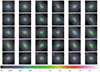 |
Fig. 1 Example of PSF reconstruction of one object, shown in logarithm scale. Panels show the PSF of each observation in the energy of 1 keV and 2 keV, except for the last four panels (panels A, B, C, and D). Panels A and B are the combined PSF weighted with exposure map in 1 keV and 2 keV, separately. In panel C, the PSF image in 1 keV and the PSF image in 2 keV are combined. Panel D shows the combined PSF image multiplied by the source count, as the final PSF image. |
3.2 Redshift estimation
To validate the existence of an X-ray extended cluster, we need to find an over-density of galaxies at the same redshift layer.
When the spatial distribution of this set of galaxies matches the X-ray contour well, we take them as the cluster members and estimate the cluster redshift with their redshifts. The redshifts of galaxies were taken from the literature. The spec-troscopic redshifts of galaxies were obtained from the Herschel Extragalactic Legacy Project (HELP), the Sloan Digital Sky Survey (SDSS) DR17, the Dark Energy Spectroscopic Instrument (DESI), the VIMOS Public Extragalactic Redshift Survey (VIPERS), the Galaxy And Mass Assembly (GAMA), the Two Micron All Sky Survey Photometric Redshift catalog (2MPZ), PRIsm MUlti-object Survey (PRIMUS), the VIMOS VLT Deep Survey (VVDS), the 6dF Galaxy Survey (6dFGS), and the 2dF Galaxy Redshift Survey (2dFGRS). The photometric redshifts of galaxies are obtained from the HELP, SDSS DR17, DESI, the Hubble Ultra Deep Field (UDF) catalog, the Canada-France-Hawaii Telescope Legacy Survey (CFHTLS), and Infrared Space Observatory (ISO). Besides, we gather galaxy redshifts from the NASA Extragalactic Database (NED2). The details and references are listed in Table A.1.
Galaxies with the offset to our detections <1.5′ are considered. To remove repetitive detections across surveys, we only reserve the information of one galaxy, when more than one galaxies with offset <1″ and |∆z| < 0.001 with each other. The redshift priority decreases as the sequence of Table A.1. The galaxies from NED are given the lowest priority. The galaxies within the following areas are included in XMM-SERVS:
 (3)
(3)
The estimation of cluster redshift was estimated in the following way. In the first step, we constructed a redshift histogram of galaxies within the range of 0–1.0 and bin size of 0.01. Four peak bins, including the largest number of galaxies, were selected. For each of the four peak bins, galaxies with redshifts in the range of zpeak ± 0.015 are taken as member candidates. In Zou et al. (2021b), the normalized photometric redshift error, ∆znorm = (zphot – zspec)/(1 + zspec), has a median value of −0.010 for W-CDF-S sources, and −0.013 for ES1 sources. In the present work, the value of ±0.015 was taken as a typical redshift range of member galaxies. Then, the four peak bins were sorted with member numbers. The final average and standard deviation of the redshifts of member galaxies are obtained after the iterative 3σ clipping. The standard deviation of redshift (z_err) is set as 0.005 when it is smaller than 0.005. In this way, we were able to obtain four candidates of the cluster redshift, as well as the errors. Figures 4a and 4b are examples of the spectroscopic and photometric redshift distribution. The four vertical lines label the locations of the four candidates of the cluster redshift.
To find out the final redshift of each detection, we obtained a reconstructed X-ray image (as described in Sect. 3.1), as well as the corresponding X-ray contour. We also obtained the r-band image from Dark Energy Survey (DES). For each of the four candidate redshifts, the position of galaxies within z ± (3 × z_err) together with the X-ray contour were overlaid over the r-band image. This procedure was undertaken for spectroscopic redshifts and photometric redshifts of galaxies respectively. Figures 5a and 5b are shown as an example. The galaxies whose redshifts within ±0.015 around the four candidates of cluster redshift values are labeled with symbols.
In addition, the RGB image combining the 𝑔, r, i bands is downloaded from the DES survey3. The RGB image helps to point out galaxies with similar colors and check whether the galaxies in the specific redshift layer have consistent spatial distribution as the X-ray contour. An example of RGB image is shown in Fig. 6a.
By applying a visual check (as described in Sect. 3.3), we selected the cluster redshift out of the four photometric redshift candidate values, four spectroscopic redshift candidate values, and the redshift of the bright central galaxy. The redshift source information is listed in the column “z_src” of the final catalog, as shown in Table B.1. When we obtained the redshift and its error of the cluster, galaxies with the redshift within z ± (3 × z_err) were taken as cluster members. The number of members is also listed in the final catalog. In Figs. 4c and 5c, examples of the redshift histogram and spatial distributions of member galaxies are shown.
 |
Fig. 2 Class 1, 2, and 3 detections, along with the false detections, shown in orange circles, green diamonds, red squares, and grey dots, respectively. The classification of detections is described in Sect. 3.5. The three regions of XMM-SERVS are shown in sequence. |
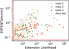 |
Fig. 3 EXTENT-Extension Likelihood distribution of detections. The symbols are the same as in Fig. 2. The selection criteria for the Extension Likelihood and EXTENT listed in Eq. (2) are shown as the vertical and horizontal red lines. |
3.3 Visual check for genuine clusters
We made visual checks of the detections to separate genuine clusters and false detections. We considered the position of members, the position of cluster detections, r-band image overlaid with X-ray contours, and the reconstructed X-ray image overlaid with X-ray contours, as well as the redshift histogram of members. The detections with the following features are taken as genuine clusters:
The X-ray contour has a regular or symmetric shape;
The X-ray emission has a strong signal-to-noise ratio;
The spatial distribution of members matches well with the X-ray contour, and one or several bright members are located at the X-ray peak;
Members have similar colors in the RGB image;
The redshift histogram of members has a Gaussian-like distribution.
An y detections without these listed features were taken to be false detections and discarded from further study. The false detections comprise detections with weak X-ray emission, X-ray emission with irregular contour, and X-ray emission on a small scale, without any obvious central bright galaxies in similar RGB colors within the cluster redshift range and without any obvious overdensity of galaxies in the cluster redshift range.
For the reliability of detected genuine clusters, we discarded also some plausible and ambiguous detections with less credibility. Probably, there are some clusters misclassified as false detections. Thus, the final cluster catalog in this work includes some newly identified clusters with comparable reliable signals, instead of being a complete cluster catalog.
In Figs. 4–7, we show sample figures and plots from the visual check for the cluster labeled “es_1”. Although the locations and redshifts of previously identified clusters are overlaid, this information is only used to classify genuine cluster detections (as described in Sect. 3.5) and not taken into account here to make the distinction between genuine clusters and false detections. In the following, we only focus on the detected genuine clusters and discard any false detections.
3.4 Characterization of genuine clusters
After the source detection, redshift estimation, and removal of false detection, we estimated the physical parameters of the cluster candidates, including the size, flux, luminosity, mass, and slope of the surface brightness profile.
3.4.1 Growth curve analysis
The growth curve analysis is made to characterize cluster detections. The integrated count rate within the radius of rsrc is plotted versus the radius, after the contribution of background and contaminates are removed. Example of the region selection and the growth curve are shown in Fig. 7.
Firstly, we masked off the contamination from the X-ray sources (listed in the last part of Table A.2) using circle masks with a radius of 15”. Some weak or compact X-ray clusters might have beeen identified as X-ray sources (especially clusters with a central AGN), therefore we did not add any masks at the central area with the radius of 20% rsrc.
The background was estimated with the average count rate in the annulus with radius from rsrc to rbgd. We separated the background area into 20 sectors and corrected the count rate in each sector with the ratio of unmasked pixels. In this way, we obtain the median and standard deviation of the total count rate for background sectors. The background sector deviated from the median with >2.3σ was removed. The final estimation of the background count rate was calculated.
In the source area, the region with a radius of 20% rsrc to rsrc is separated into 4 annuli, and further divided into 16 sectors each. In each annulus, sectors with contaminates are removed with the same procedure as the background. In the central area with a radius of 20% rsrc, emission from all pixels is considered in the growth curve. Finally, we obtain the integrated count rate for a set of radii after the removal of the background.
In the process of the growth curve, the rsrc and rbgd are usually taken as 5.0′ and 6.0′, respectively. For some complex systems, the values of rsrc and rbgd were changed manually to obtain a steady growth curve with a flat plateau outside. For some clusters, contaminates were left in the source area, worsening the performance of the growth curve. Thus, we masked off some more sectors manually, which included contaminates that were identified by a visual check.
In the growth curve (shown in Fig. 7b), the integrated count rate increases with the radius and turns into a plateau at the significant radius. Outside the significant radius, the X-ray contribution from the central source is negligible compared with the background fluctuation. Thus, we obtained the significant radius (Rsig) as the inner radius of the plateau area, and the count rate in the plateau (CRsig). These two parameters are used to characterize our clusters, as described in Sect. 3.4.2.
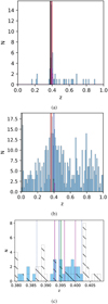 |
Fig. 4 Redshift histogram of galaxies within the offset <1.5′ of the cluster “es_1” for the visual check, as an example. Panel a: spectroscopic redshift within 0-1.0. The bin width is 0.01. The blue, red, brown, and black vertical lines show the location of the four highest bins. The magenta and green histograms are for the redshifts of previous ICM-detected clusters and OPT/IR clusters with offset <3.0′, respectively. Panel b: photometric redshift within 0-1.0. Symbols are the same as in Fig. 4a. Panel c: redshift histogram of member galaxies within zpeak ± 0.015, shown in 30 bins. Blue bins for spectroscopic red-shifts, and black hatched bins for photometric redshifts. The blue solid and blue dotted vertical lines show the cluster redshift and its 1σ range. The magenta and green vertical lines are the redshifts of previous ICM-detected clusters and OPT/IR clusters within 3.0′. |
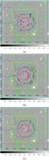 |
Fig. 5 Spatial distribution of galaxies surrounding the cluster “es_1” in a specific redshift layer corresponding to the three panels in Fig. 4, in sequence. Panel a: r-band image in log scale, overlaid with galaxies redshifts within ±0.015 around the four highest redshift bins (blue “x”, red “+”, brown diamond, and black box in sequence) in Fig. 4a, X-ray contour in green, location of previously identified clusters (referring to Sect. 3.5, magenta circle for ICM-detected cluster, blue circle for OPT/IR cluster, radius as the smaller value of 0.5 Mpc and 1.0′), the location of XVXGC cluster (red circle with a radius of “EXTENT” value), and the white box with the size of 5′ × 5′, the yellow box with the size of 3.0′ × 3.0′. Panel b: same as Fig. 5a, but for the photometric redshifts. Panel c: same as Fig. 5a, but overlaid only the location of member galaxies (blue “x” for spectroscopic redshift, red “+” for photometric redshift). |
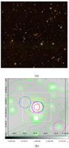 |
Fig. 6 Image of the cluster “es_1” in RGB color and reconstructed X-ray image. Panel a: RGB image combining 𝑔, r, i bands from DES survey, in the size of 10′ × 10′. Panel b: reconstructed X-ray image in log scale, overlaid with X-ray contours in green, and previously identified clusters whose symbols are consistent with Fig. 5a. The size of the white and yellow boxes are the same as Fig. 5a. The size of black box is 10′ × 10′. |
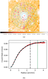 |
Fig. 7 Region selection and growth curve for the cluster “es_1”, as an example. Panel a: the reconstructed X-ray image in log scale, overlaid with the source regions (cyan sectors) and background regions (green sectors) for the growth curve analysis. The red circles outside the central cyan circle, and red dashed sectors are masks for contaminates. Panel b: growth curve plot, with the integrated count rate versus the radius shown in red (1 σ range in pink), where black dot-dashed and green dashed vertical lines label the R500 and the significant radius, and the horizontal dotted line for the count rate in the plateau. The black dashed curve is the best-fitting model for the growth curve, with the β = 0.683 for this source. The model with typical β = 2/3 is plotted in a cyan dotted curve as a comparison. |
3.4.2 Flux, luminosity, and mass estimation
In this subsection, we describe our estimation of the flux, luminosity, and mass for each cluster, with the value of significant radius and the count rate in the plateau from the growth curve analysis. We give our main steps below.
Firstly, we assumed R500 equals the value of Rsig. The reason for this assumption is the X-ray emission within the radius of R500 in general dominates in the observation. With the redshift known, the R500 in the unit of arcmin can be converted to the physical radius in the unit of Mpc. As we know, the definition of R500 is the radius where the included average density is 500 times the critical density of the universe at the redshift. Thus, the total mass within R500 is obtained as
 (4)
(4)
Secondly, we derive the bolometric X-ray luminosity (Lx,bol) and temperature (Tx), using scaling relations from the Eqs. (23)–(26) of Reichert et al. (2011). With the APEC model, we can further obtain the luminosity within R500 in the rest-frame [0.5– 2.0] keV band (L500), as well as the flux in the band (F500), with the k-correction taken into account. Then, the conversion factor between the count rate and flux is obtained by averaging the values for instruments of MOS1, MOS2, and PN with PIMMS4 (Mukai 1993). Thus, we can derive the expected total count rate within R500 as CR500. In this step, the absorption of neutral hydrogen was obtained from the HI4PI survey (HI4PI Collaboration 2016) and the metallicity was fixed as 0.3 Z⊙.
Assuming the typical β-profile (Eq. (1)) with β = 2/3, the expected total count rate within the significant radius (CRsig,est) can be calculated from the value of Rsig, R500, and CR500. Then, we change the value of R500 and iteratively repeat the steps above in this section until the value of CRsig,est equal to the observed value of CRsig. This way, we obtained R500 and CR500. The 1σ error of CRsįg was estimated with the count rate uncertainty in the plateau of the growth curve. Then the error of CR500 was obtained by the linear interpolation of the count rate uncertainty in the growth curve at the radius of R500. The error of R500 was estimated with σR500/R500 = σCR500/CR500. Thus, all values of R500, σR500, CR500, σCR500 were obtained.
In the next step, the M500 value was estimated based on the value of R500 (as in Eq. (4)). Then, the temperature of ICM (Tx) was derived from M500 with the aforementioned scaling relation. In the other way, the F500 in the band of [0.5–2.0] keV was estimated with CR500, then L500 in its rest-frame [0.5–2.0] keV was calculated from F500 with the k-correction. The errors of these parameters were estimated from the errors of R500 and CR500, with the error propagation laws.
3.4.3 β-value from the growth curve
As mentioned in Sect. 3.1, the typical surface-brightness profile of cluster can be described with β-model (Eq. (1)), while the β value reflects the steepness of the profile. The larger β value, the steeper profile. In this section, we describe how we estimated the β value for each detection with the growth curve.
The PSF of XMM-Newton EPIC instruments varies largely with the energy, off-axis angle, and instrument. Read et al. (2011) provided a fully 2D characterization of the PSF as a function of energy and off-axis angle, for each EPIC instrument. The PSF of PN can be described using a 2D King profile (B(r), Eq. (5)); whereas a subsequent 2D Gaussian function (G(r), Eq. (6)) is needed for MOS1 and MOS2 for the excess emission at the core. In the 2D King profile, r0 is the core radius, α is the power-law slope, e is the ellipticity, and θ is the angle of ellipticity. In the 2D Gaussian function, the FWHM is the full width at half maximum and “Norm” is the normalization ratio of the Gaussian peak to the King peak. This is computed as follows:
![Mathematical equation: $B(r) = {A \over {{{\left[ {1 + {{\left( {r/{r_0}} \right)}^2}} \right]}^\alpha }}},$](/articles/aa/full_html/2024/11/aa51064-24/aa51064-24-eq5.png)
![Mathematical equation: $r(x,y,\theta ) = \sqrt {\left[ {{{(x\cos \theta + y\sin \theta )}^2}} \right] + {{{{(y\cos \theta - x\sin \theta )}^2}} \over {{{(1 - )}^2}}}} ,$](/articles/aa/full_html/2024/11/aa51064-24/aa51064-24-eq6.png) (5)
(5)
 (6)
(6)
Some other features are coming from the support structure features, including the radially dependentprimary andsecondary spoke structures, as well as the large-scale azimuthal modulation. However, the X-ray data used in this work is mosaicked from multiple observations of all three EPIC instruments. Thus, it is difficult to model these spatial-dependent features.
As described in Read et al. (2011), the PSF parameters for the MOS1, MOS2, and PN are provided in the ELLBETA parameters of the files, XRT1_XPSF_0016.CCF, XRT2_XPSF_0016.CCF, XRT3_XPSF_0018.CCF. The best sets of PSF parameters are provided across eight energy values (0.1 keV, 1.5 keV, 2.75 keV, 4.25 keV, 6 keV, 8 keV, 10.25 keV, 15 keV) with seven off-axis angles (0′, 1′, 3′, 6′, 9′, 12′, 15′). The off-axis angle of 1′ is not provided for MOS1. The PSF parameters in 1 .5 keV with the off-axis angle of 9′ are taken as the representative PSF of our data.
There are five parameters in the PSF model: r0, α, and ϵ of the 2D King model and the FWHM and Norm of the 2D Gaussian model. The θ value in the 2-D King model is always 0. The values of r0 and α of MOS1, MOS2, and PN, are averaged to obtain their values of final PSF. There is no asymmetric information included in the growth curve, thus the ellipticity is set to 0. However, the ellipticity will systematically enlarge the PSF size in mosaicked images, and might bring some bias to our estimation of β-model parameters in some way. Because only MOS1 and MOS2 have a 2D Gaussian component, we take the average FWHM of MOS1 and MOS2 as the final FWHM parameter and divide the sum of their Norm values by 3 as the final Norm parameter. The final set of PSF parameters are (r0, α, ϵ, FWHM, Norm) = (7.605″, 1.624, 0, 4.304″, 0.582).
In the fitting of the growth curve, the β-model (Eq. (1)) was convolved with the PSF model. The parameters were estimated with the Markov chain Monte Carlo (MCMC) fitting using the EMCEE package5 (Foreman-Mackey et al. 2013). The β value was constrained within the range of 0.3-1.0. We used 50 chains with the original length of 5000 steps each and discarded the first 2000 steps.
The last panel of Fig. 8 shows the posterior distribution of β-value. Although there are peaks at the high and low ends, representing ultra-steep or ultra-flat surface brightness profiles, the newly identified X-ray clusters systematically have lower β-value than previously identified X-ray clusters. This tendency is consistent with the RXGCC sample (Xu et al. 2022). Their flat X-ray profile might be a reason for the incomplete detection in previous works about X-ray cluster identification.
3.5 Classification of genuine clusters
After the detection and characterization, we checked whether cluster candidates had been detected previously. We refer to both X-ray clusters and SZ clusters as “ICM-detected clusters” and refer to both optical and IR clusters as “OPT/IR clusters”. We collected the literature and NED database values for previously identified clusters, listed in Table A.2. For convenience, we refer to clusters from literature or NED as “clusters from the literature” in in this paper.
In the NED database, we take systems with the following types as clusters, cluster of galaxies, group of galaxies. Out of the NED clusters, systems with names beginning with the following were taken as ICM-detected clusters: 3XLSS, ACT-CL, ECDF-S, RCC, RzCS, SMACS, SPT- CL, SXDF, X-CLASS, XLSS, XLSSC, XLSSsC, XMM-LSS, XMMU, XMMXCS, and XXL-N. Otherwise, systems were taken as OPT/IR clusters, with names beginning with 400d, ABELL, CCPC-z, CDFS:[AMI2005], CDGS, CFHT-D CL, CFHT-W CL, CFHTLS CL, CFHTLS c, CFHTLS:[DAC2011] W1, CFHTLS:[SMD2018a] W1, CL, CVB, ClG, G3Cv10, HSCS, JKCS, LCLG, MZ, PGC1, RCS1, redMaPPer, RM, SCG, SL, SWIRE CL, SXDS:[MHE2007], SpARCS, UDSC, WHL, [AMP2011], [DJ2014], [DRV2022], [HMC2016], [LIK2015], [LMR2016], [MOH2018], [MSP2015], [PCG2016], [SCP2009], [TKO2016], [VCB2006], [WH2018], and [YHW2022].
Besides the listed cluster catalogs in Table A.2, there are some more catalogs that ought to be taken into account. However, no clusters from these catalogs are located within the coverage of XMM-SERVS survey (Eq. (3)). These include the catalogs of X-ray clusters identified with ROSAT data (Ebeling et al. 1996; Ledlow et al. 2003; Xu et al. 2022) and those with XMM-Newton and S DS S data (Takey et al. 2011, 2013, 2014, 2016), catalogs of SZ clusters identified using the SPT data (Huang et al. 2020; Bleem et al. 2024), ACT data (Marriage et al. 2011; Hasselfield et al. 2013), and Planck data (Planck Collaboration VIII 2011).
We cross-matched the detections with previously identified galaxy clusters with an offset of <3.0′. In this process, we did not set a threshold of redshift differences, with an aim to avoid the inaccurate estimation of cluster redshift. The position of clusters, together with the X-ray contour and member galaxies, are overlaid on the r-band image. One example is shown in Fig. 5. By visual check, only clusters with positions matching well with the X-ray contour are taken as the counterparts of our detections.
In Fig. 9, we show the distribution of position offsets and redshift differences between our clusters and previously detected cluster counterparts. Most matched clusters have an offset smaller than 0.5′. The redshift differences are always <0.2, except for 5 ICM-detected clusters, and 2 OPT/IR clusters.
With a visual check, as shown in (Figs. 4–7), we classified our detections for genuine clusters into previous ICM-detected clusters (class 3), previous OPT/IR clusters (class 2), and new clusters (class 1). The detections with both previous ICM-detected clusters and OPT/IR clusters as counterparts are classified as class 3. The locations of these detections for genuine clusters are shown in Fig. 2. In Fig. 3, their distribution in EXTENT-Extension likelihood parameter space is shown. Finally, the numbers of clusters in classes are listed in Table 1. We compile the class 1, class 2, and class 3 detections into the final catalog, as described in Sect. 4. In later sections, we only discuss these cluster detections.
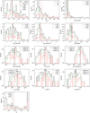 |
Fig. 8 Histogram of parameters. The red dashed histogram for class 3 clusters, and green dotted histogram for the “class 1 + class 2” and the black solid histogram for the whole XVXGC sample. The red dashed, green dotted, and black solid vertical lines give the median values of the corresponding sample. |
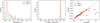 |
Fig. 9 Distribution of position offset and redshift difference for the cross-matched clusters between XVXGC and literature (left and middle panels, respectively). The right panel is the redshift comparison. The “z,literature” in the panels indicates the redshifts from the literature. Red solid histogram and red squares for class 3, green dot histogram, and green diamonds for class 2. |
Cluster numbers in classes and regions.
4 Result and discussion
4.1 The catalog
In this work, we gather detections of 141 X-ray extended galaxy clusters, named the XMM-SERVS X-ray eXtended Galaxy Cluster catalog (XVXGC). The catalog and figures for each source are available at CDS and the XVXGC webpage6 respectively. In Table B.1, the first two entries are shown for the table format. In Figs. 4–7, we show the figure data for the cluster labeled “es_1” in the catalog, as an example.
In the XVXGC catalog, we list the following parameters for each cluster: name, position, the classification, number of member galaxies, redshift, redshift error, redshift source, extension likelihood, EXTENT value, significant radius (Rsig), count rate in the plateau of the growth curve (CRsig) and its error, cluster radius (R500), total count rate within R500 (CR500), total flux (F500), luminosity (L500), temperature of ICM (Tx), and mass within R500 (M500), together with their corresponding 1σ errors. Furthermore, we list the β-value and the core radius Rc, as well as their lower and upper 1σ error. The F500 is estimated in the band of [0.5–2.0] keV and L500 in the rest-frame [0.5–2.0] keV.
In the XVXGC catalog, there are new 48 clusters (class 1), 40 previous OPT/IR clusters (class 2), and 53 previous ICM-detected clusters (class 3). In Fig. 8, we plot the histogram of parameters for the XVXGC sample, “class 1 + class 2”, and class 3 samples, with the median value overlaid. These median values are also listed in Table 2. Besides, the median value of the 1σ error of R500 is 0.028 Mpc, CR500 error as 0.001/s, F500 error as 8.524 × 10⁻¹⁶ erg/s/cm2, L500 error as 3.862 × 1041 erg/s, Tx error as 0.104 keV, and M500 error as 7.512 × 10¹² M⊙. In addition, we show the ratio between the estimated parameter and its error in Table 3. From the figure and tables, we find:
Redshifts of XVXGC sample go from 0.0539 to 0.9784, with most detections with z < 0.6;
The number of members are in range of 8–120, with median value of 27;
The median radius of XVXGC clusters is 0.315’, 2.455’, 1.576’, 0.459 Mpc for Rc, Rsig, R500, and R500;
The median count rate within Rsig and R500 is 9.249 × 10⁻³ count/s and 9.269 × 10⁻³ count/s separately;
The median flux, luminosity, gas temperature, and mass within R500 is 1.447 × 10⁻¹⁴ erg/s/cm2, 5.917 × 1042 erg/s, 1.358 keV, 3.866 × 10¹³ M⊙. The histograms in the logarithm of these parameters are nearly symmetric;
A large fraction of clusters are with M500 < 1014 M⊙, and should be classified as galaxy groups instead of galaxy clusters. However, in this work, we use the term “galaxy clusters” representing both types for convenience;
Except for values at the high and low β value end, representing ultra-steep or ultra-flat surface brightness profiles, the distribution of β-value peaks at the value of ~0.5. It corresponds to a much flatter surface brightness profile than the typical cluster profile;
The class 1, 2, and 3 samples are found to overlap with each other in all parameters generally, but the “class 1+2” sample seems to always take a comparably larger percentage close to the lowest end;
Compared with class 3 clusters, the “class 1 + class 2” sample tends to be less bright and less massive, with a flatter X-ray surface brightness profile.
Median value of parameters.
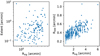 |
Fig. 10 Distribution of radius estimations, Rsig , EXTENT, and R500. The significant radius, Rsig, is the radius when the growth curve turns into a plateau (Sect. 3.4.1). The EXTENT is the estimation of the core radius in the β-model using the maximum likelihood fitting (Sect. 3.1). The R500 value is the radius where the average density inside is 500 times the critical density (Sect. 3.4.2). |
4.2 Distribution of size estimations
In Fig. 10, we show the distribution of size estimations. The significant radius is the outer boundary when the X-ray emission from the cluster is higher than the background fluctuation. The EXTENT value is estimated from the maximum likelihood fitting method, as a characteristic radius for extended sources. It is comparable with the significant radius and has a comparable weak correlation with the significant radius. However, the EXTENT parameter is only used in the separation of extended and point-like sources and the threshold of EXTENT value (4″) is small for the detection of a large fraction of extended sources.
In addition, the R500 is the radius for physical parameters of clusters. In the figure, we find the R500 is always lower than the significant radius. It means in the analysis, all X-ray emission in the region of R500 are considered.
Median ratio between parameters and corresponding error.
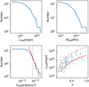 |
Fig. 11 Cumulative number of luminosity, mass, and flux, as well as the relation between luminosity and redshift. In the lower-left panel, the dashed line indicates the line with the slope of –1.5 and normalized at F500 = 4 × 10–14 erg/s/cm2. In the lower-right panel, the dashed and dotted curve corresponds to the F500 of 4 × 10–15 erg/s/cm2, and 4 × 10–14 erg/s/cm2, respectively. |
4.3 Flux function, luminosity function, mass function
In the top-left, top-right, and lower-left panels of Fig. 11, the cumulative number of luminosity, mass, and flux is shown as a representation for the luminosity, mass, and flux function; however, no selection functions have been corrected here. In the lower-left panel, the dashed line indicates the slope of –1.5 for the Euclidean universe where clusters are uniformly distributed. The line is normalized with the curve at 4 × 10–14 erg/s/cm2. It matches with the curve at >4 × 10–14 erg/s/cm2 well, which is shown with the vertical line. This indicates our high completeness for brighter clusters. On the other hand, our detection of fainter clusters has a lower completeness. This catalog is not a complete catalog of bright clusters, but instead a complementary catalog of clusters with some newly identified clusters with our dedicated algorithm. In the histogram of F500 in Fig. 8, there are some “class 1+2” clusters with >4 × 10–14 erg/s/cm2. The newly ICM-detected bright clusters are possible evidence of unexpected incompleteness in previous works.
In addition, the flux of 4 × 10⁻¹⁵ erg/s/cm2, and 4 × 10⁻¹⁴ erg/s/cm2 are overlaid into the relation of luminosity and redshift (lower right panel of Fig. 11). We find XVXGC clusters are mainly within this flux range up to the redshift of ~1.0, with some fainter clusters mainly detected at low redshift of z < 0.5.
4.4 The offset to the X-ray sources
To quantify the effect of X-ray sources on our detections, we cross-matched the XVXGC clusters with X-ray sources identified from XMM-Newton data, listed in the last part of Table A.2. The offset threshold is set as 0.315′, which is the median value of the core radius of XVXGC clusters (Table 2). There are 53 “class 1 + class 2” and 35 ‘class 3’ XVXGC clusters with central X-ray sources and the offset distribution is shown in Fig. 12.
In the work by Ni et al. (2021) and Chen et al. (2018), the average number density of X-ray sources identified in the XMM- SERVS survey is ~0.36 in each square arcmin. Then, the total area of 141 circles with a radius of 0.315’ is ~44 square arcmin. Thus, there are ~16 X-ray sources within an offset of <0.315′ of XVXGC clusters from purely projection effect, assuming the X-ray sources are distributed randomly and without correlation with clusters. Thus, out of the total 88 “class 1+2” clusters, there are 53 ones with central X-ray sources. In these 53 clusters, after removing the ~16 ones with projected X-ray sources, there are 37 “class 1+2” clusters with physical combination with X-ray sources. It means there are roughly 51 newly ICM-detected clusters without central X-ray sources, taking ~58% of “class 1+2”. In Fig. 13, the parameters are compared for the “class 1+2” sample with and without central X-ray sources, and no systematic differences are found between the samples.
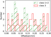 |
Fig. 12 Histogram of offset between XVXGC clusters and X-ray sources. The red solid histogram is for class 3 clusters and the green dotted histogram is for the “class 1 + class 2” clusters. |
4.5 Physical parameter comparison with previous X-ray clusters
We cross-matched the XVXGC clusters with X-ray clusters from the literature, including those identified in (Bulbul et al. 2024; Koulouridis et al. 2021; Finoguenov et al. 2020; Adami et al. 2018; Wen et al. 2018; Finoguenov et al. 2015). The cross-matching criteria are set as offset smaller than 1.0 arcmin for a robust result. In the XMM-LSS, W-CDF-S, and ES1 regions, there are respectively 30, 4, and 4 XVXGC clusters with X-ray detected clusters reported in these works. The comparison of physical parameters of z, R500, log(L500), log(M500), and log(F500) are shown in Fig. 14. We fit the relation between our estimation and literature results with a linear function: Par,XVXGC = k × Par,literature + b. The fitting was done using the Markov chain Monte Carlo (MCMC) technique. The best-fitting parameters and their 1σ error are listed in Table 4. In addition, the Kolmogorov-Smirnov test (K–S test) statistic D and the p-value are also listed in Table 4.
We found that our estimations of z, R500, L500, M500, and F500 are all positively correlated with literature results. In particular, the redshifts are tightly consistent with the literature values, although there are two outliers. These outliers likely result from the different methods to identify member galaxies. In our estimation of R500, clusters with R500 > 0.75 Mpc from literature is under-estimated by ~50%. This is possibly a limitation of our method for parameter estimation with the growth curve analysis, as described in Sect. 3.4.2. In the growth curve analysis, the region area considered is limited, because the projected contaminates are more difficult to remove in a larger region.
However, our estimations of L500, M500, and F500 all have a nice linear relation with the literature results, although there is some scatter involved. The possible reasons for the scatter among the parameters include limitations in the scope of the cross-matched sample, the X-ray data used to identify clusters, parameter estimation methods, and the different scaling relations used. In addition, in the cross-matching with the literature, not all of these parameters are provided by each referenced catalog; thus, the number of data points given in the panels of Fig. 14 varies.
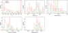 |
Fig. 13 Parameter comparison for the “class 1+2” sample with and without central X-ray sources detected. |
5 Conclusion
In this work, we present the detection of X-ray extended clusters based on the XMM-SERVS data (Chen et al. 2018; Ni et al. 2021) with the wavelet-based detection method (Pacaud et al. 2006; Xu et al. 2018). We identified 141 clusters, named the XMM-SERVS X-ray eXtended Galaxy Cluster (XVXGC) catalog. There are 48 new clusters, 40 previously identified OPT/IR clusters without previous ICM-based identification, and 53 previous ICM-identified clusters. Compared with previous ICM-detected clusters, our newly ICM-detected clusters tend to be fainter, with a flatter X-ray surface brightness profile.
Out of 88 first ICM-detected clusters, there are ~58% without physical correlated central X-ray sources. Thus, there are roughly 51 clusters detected with their ICM emission for the first time. In addition, by comparing physical parameters with counterparts in previous X-ray cluster catalogs, we find XVXGC has a good redshift and physical parameter estimations.
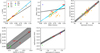 |
Fig. 14 Comparison of physical parameters in XVXGC catalog and other X-ray cluster catalogs. The grey dashed lines show a 1:1 relation. The best-fitting linear function is shown in a black line, with the 1σ error shown in the grey region. The parameter values of the best-fitting linear model and K-S test parameters are shown in Table 4. In the first panel, after removing two outliers at the lower-right part, a second best-fitting model is overlaid as the blue dotted line together with the cyan shade for its 1σ error. In the second panel, the second best-fitting model is also overlaid when the outlier at the upper-left part is removed. |
Data availability
Full Table B.1 is available at the CDS via anonymous ftp to cdsarc.cds.unistra.fr (130.79.128.5) or via https://cdsarc.cds.unistra.fr/viz-bin/cat/J/A+A/691/A300.
Acknowledgements
We acknowledge support from the National Key R&D Program of China (2021YFA1600404, 2022YFF0503403, 2022YFF0503401), National Nature Science Foundation of China (Nos 11988101, 12022306, 12203063), the China Manned Space Project (CMS-CSST-2021-B01, CMS- CSST-2021-A01, CMS-CSST-2021-A05, CMS-CSST-2021-A06, CMS-CSST- 2021-A07), and the National Science Foundation of China (12225301), the support from the Ministry of Science and Technology of China (Nos. 2020SKA0110100), CAS Project for Young Scientists in Basic Research (No. YSBR-062), and the support from K.C. Wong Education Foundation. BL acknowledges financial support from the National Natural Science Foundation of China grant 11991053. CZ acknowledges support from Zhejiang Provincial Natural Science Foundation of China under grant No. LQ24A030001. W.X. thanks Thomas H. Reiprich, Florian Pacaud, Miriam E. Ramos-Ceja, Ang Liu, Mingyang Zhuang, Shi Li for useful discussion during the development of this paper. This paper uses data from the VIMOS Public Extragalactic Redshift Survey (VIPERS). VIPERS has been performed using the ESO Very Large Telescope, under the “Large Programme” 182.A-0886. The participating institutions and funding agencies are listed at http://vipers.inaf.it.
Appendix A Collection of galaxy redshifts, galaxy clusters, and identified X-ray sources
In Table A.1, we list galaxy redshifts from literature and NED database. In Table A.2, the galaxy clusters identified in bands are listed in the first three parts, while the identified X-ray sources are shown in the last part.
Overview of galaxy redshifts from literature and NED database.
Overview of previously identified clusters and X-ray sources.
Appendix B XVXGC cluster catalog
In Table B.1, we show the first two entries of XVXGC catalog for its format. The entire table is released on CDS.
First two entries in the XVXGC catalog as an example.
References
- Abdurro’uf, Accetta, K., Aerts, C., et al. 2022, ApJS, 259, 35 [NASA ADS] [CrossRef] [Google Scholar]
- Abell, G. O. 1958, ApJS, 3, 211 [NASA ADS] [CrossRef] [Google Scholar]
- Abell, G. O., Corwin, Jr., H. G., & Olowin, R. P. 1989, ApJS, 70, 1 [NASA ADS] [CrossRef] [Google Scholar]
- Adami, C., Giles, P., Koulouridis, E., et al. 2018, A&A, 620, A5 [NASA ADS] [CrossRef] [EDP Sciences] [Google Scholar]
- Allen, S. W., Evrard, A. E., & Mantz, A. B. 2011, ARA&A, 49, 409 [Google Scholar]
- Andrade-Santos, F., Jones, C., Forman, W. R., et al. 2017, ApJ, 843, 76 [Google Scholar]
- Baldry, I. K., Liske, J., Brown, M. J. I., et al. 2018, MNRAS, 474, 3875 [Google Scholar]
- Berlind, A. A., Frieman, J., Weinberg, D. H., et al. 2006, ApJS, 167, 1 [Google Scholar]
- Bertin, E., & Arnouts, S. 1996, A&AS, 117, 393 [NASA ADS] [CrossRef] [EDP Sciences] [Google Scholar]
- Bilicki, M., Jarrett, T. H., Peacock, J. A., Cluver, M. E., & Steward, L. 2014, ApJS, 210, 9 [Google Scholar]
- Bleem, L. E., Stalder, B., de Haan, T., et al. 2015, ApJS, 216, 27 [Google Scholar]
- Bleem, L. E., Bocquet, S., Stalder, B., et al. 2020, ApJS, 247, 25 [Google Scholar]
- Bleem, L. E., Klein, M., Abbot, T. M. C., et al. 2024, Open J. Astrophys., 7, 13 [CrossRef] [Google Scholar]
- Bocquet, S., Grandis, S., Bleem, L. E., et al. 2024, Phys. Rev. D, 110, 083510 [NASA ADS] [CrossRef] [Google Scholar]
- Böhringer, H., Schuecker, P., Guzzo, L., et al. 2004, A&A, 425, 367 [NASA ADS] [CrossRef] [EDP Sciences] [Google Scholar]
- Borgani, S., & Kravtsov, A. 2011, Adv. Sci. Lett., 4, 204 [Google Scholar]
- Bulbul, E., Liu, A., Kluge, M., et al. 2024, A&A, 685, A106 [NASA ADS] [CrossRef] [EDP Sciences] [Google Scholar]
- Burenin, R. A., Vikhlinin, A., Hornstrup, A., et al. 2007, ApJS, 172, 561 [Google Scholar]
- Butcher, H., & Oemler, A., J. 1984, ApJ, 285, 426 [NASA ADS] [CrossRef] [Google Scholar]
- Cash, W. 1979, ApJ, 228, 939 [Google Scholar]
- Cavagnolo, K. W., Donahue, M., Voit, G. M., & Sun, M. 2009, ApJS, 182, 12 [Google Scholar]
- Chen, C. T. J., Brandt, W. N., Luo, B., et al. 2018, MNRAS, 478, 2132 [NASA ADS] [CrossRef] [Google Scholar]
- Chiappetti, L., Clerc, N., Pacaud, F., et al. 2013, MNRAS, 429, 1652 [NASA ADS] [CrossRef] [Google Scholar]
- Chiu, I. N., Klein, M., Mohr, J., & Bocquet, S. 2023, MNRAS, 522, 1601 [NASA ADS] [CrossRef] [Google Scholar]
- Clerc, N., Sadibekova, T., Pierre, M., et al. 2012, MNRAS, 423, 3561 [NASA ADS] [CrossRef] [Google Scholar]
- Coil, A. L., Blanton, M. R., Burles, S. M., et al. 2011, ApJ, 741, 8 [Google Scholar]
- Colless, M., Dalton, G., Maddox, S., et al. 2001, MNRAS, 328, 1039 [Google Scholar]
- Costanzi, M., Saro, A., Bocquet, S., et al. 2021, Phys. Rev. D, 103, 043522 [Google Scholar]
- Coupon, J., Ilbert, O., Kilbinger, M., et al. 2009, A&A, 500, 981 [NASA ADS] [CrossRef] [EDP Sciences] [Google Scholar]
- Dehghan, S., & Johnston-Hollitt, M. 2014, AJ, 147, 52 [NASA ADS] [CrossRef] [Google Scholar]
- Ebeling, H., Voges, W., Bohringer, H., et al. 1996, MNRAS, 281, 799 [NASA ADS] [CrossRef] [Google Scholar]
- Eckert, D., Molendi, S., & Paltani, S. 2011, A&A, 526, A79 [NASA ADS] [CrossRef] [EDP Sciences] [Google Scholar]
- Finoguenov, A., Guzzo, L., Hasinger, G., et al. 2007, ApJS, 172, 182 [Google Scholar]
- Finoguenov, A., Watson, M. G., Tanaka, M., et al. 2010, MNRAS, 403, 2063 [NASA ADS] [CrossRef] [Google Scholar]
- Finoguenov, A., Tanaka, M., Cooper, M., et al. 2015, A&A, 576, A130 [NASA ADS] [CrossRef] [EDP Sciences] [Google Scholar]
- Finoguenov, A., Rykoff, E., Clerc, N., et al. 2020, A&A, 638, A114 [NASA ADS] [CrossRef] [EDP Sciences] [Google Scholar]
- Foreman-Mackey, D., Hogg, D. W., Lang, D., & Goodman, J. 2013, PASP, 125, 306 [Google Scholar]
- Gabriel, C., Denby, M., Fyfe, D. J., et al. 2004, in Astronomical Data Analysis Software and Systems (ADASS) XIII, eds. F. Ochsenbein, M. G. Allen, & D. Egret, Astronomical Society of the Pacific Conference Series, 314, 759 [NASA ADS] [Google Scholar]
- Ghirardini, V., Bulbul, E., Artis, E., et al. 2024, A&A, 689, A298 [NASA ADS] [CrossRef] [EDP Sciences] [Google Scholar]
- Gully, H., Hatch, N., Bahé, Y., et al. 2024, MNRAS, 527, 10680 [Google Scholar]
- Hasselfield, M., Hilton, M., Marriage, T. A., et al. 2013, J. Cosmology Astropart. Phys., 7, 008 [CrossRef] [Google Scholar]
- HI4PI Collaboration (Ben Bekhti, N., et al.) 2016, A&A, 594, A116 [NASA ADS] [CrossRef] [EDP Sciences] [Google Scholar]
- Hilton, M., Hasselfield, M., Sifón, C., et al. 2018, ApJS, 235, 20 [Google Scholar]
- Hilton, M., Sifón, C., Naess, S., et al. 2021, ApJS, 253, 3 [Google Scholar]
- Huang, N., Bleem, L. E., Stalder, B., et al. 2020, AJ, 159, 110 [Google Scholar]
- Ilbert, O., Arnouts, S., McCracken, H. J., et al. 2006, A&A, 457, 841 [NASA ADS] [CrossRef] [EDP Sciences] [Google Scholar]
- Jones, D. H., Saunders, W., Colless, M., et al. 2004, MNRAS, 355, 747 [NASA ADS] [CrossRef] [Google Scholar]
- Klein, M., Grandis, S., Mohr, J. J., et al. 2019, MNRAS, 488, 739 [Google Scholar]
- Klein, M., Hernández-Lang, D., Mohr, J. J., Bocquet, S., & Singh, A. 2023, MNRAS, 526, 3757 [NASA ADS] [CrossRef] [Google Scholar]
- Koulouridis, E., Clerc, N., Sadibekova, T., et al. 2021, A&A, 652, A12 [NASA ADS] [CrossRef] [EDP Sciences] [Google Scholar]
- La Franca, F., Gruppioni, C., Matute, I., et al. 2004, AJ, 127, 3075 [NASA ADS] [CrossRef] [Google Scholar]
- Le Fèvre, O., Cassata, P., Cucciati, O., et al. 2013, A&A, 559, A14 [Google Scholar]
- Ledlow, M. J., Voges, W., Owen, F. N., & Burns, J. O. 2003, AJ, 126, 2740 [NASA ADS] [CrossRef] [Google Scholar]
- Lewis, I., Balogh, M., De Propris, R., et al. 2002, MNRAS, 334, 673 [NASA ADS] [CrossRef] [Google Scholar]
- Mantz, A., Allen, S. W., Rapetti, D., & Ebeling, H. 2010, MNRAS, 406, 1759 [NASA ADS] [Google Scholar]
- Marriage, T. A., Acquaviva, V., Ade, P. A. R., et al. 2011, ApJ, 737, 61 [Google Scholar]
- McClintock, T., Varga, T. N., Gruen, D., et al. 2019, MNRAS, 482, 1352 [Google Scholar]
- Mehrtens, N., Romer, A. K., Hilton, M., et al. 2012, MNRAS, 423, 1024 [NASA ADS] [CrossRef] [Google Scholar]
- Mukai, K. 1993, Legacy, 3, 21 [Google Scholar]
- Ni, Q., Timlin, J., Brandt, W. N., & Yang, G. 2019, RNAAS, 3, 5 [NASA ADS] [Google Scholar]
- Ni, Q., Brandt, W. N., Chen, C.-T., et al. 2021, ApJS, 256, 21 [CrossRef] [Google Scholar]
- Oguri, M. 2014, MNRAS, 444, 147 [NASA ADS] [CrossRef] [Google Scholar]
- Oguri, M., Lin, Y.-T., Lin, S.-C., et al. 2018, PASJ, 70, S20 [NASA ADS] [Google Scholar]
- Pacaud, F., Pierre, M., Refregier, A., et al. 2006, MNRAS, 372, 578 [NASA ADS] [CrossRef] [Google Scholar]
- Pacaud, F., Clerc, N., Giles, P. A., et al. 2016, A&A, 592, A2 [NASA ADS] [CrossRef] [EDP Sciences] [Google Scholar]
- Peng, Y.-j., Lilly, S. J., Kovac, K., et al. 2010, ApJ, 721, 193 [NASA ADS] [CrossRef] [Google Scholar]
- Pierre, M., Adami, C., Birkinshaw, M., et al. 2017, Astron. Nachr., 338, 334 [NASA ADS] [CrossRef] [Google Scholar]
- Piffaretti, R., Arnaud, M., Pratt, G. W., Pointecouteau, E., & Melin, J.-B. 2011, A&A, 534, A109 [NASA ADS] [CrossRef] [EDP Sciences] [Google Scholar]
- Planck Collaboration VIII. 2011, A&A, 536, A8 [NASA ADS] [CrossRef] [EDP Sciences] [Google Scholar]
- Planck Collaboration XXIX. 2014, A&A, 571, A29 [NASA ADS] [CrossRef] [EDP Sciences] [Google Scholar]
- Planck Collaboration XXXII. 2015, A&A, 581, A14 [NASA ADS] [CrossRef] [EDP Sciences] [Google Scholar]
- Planck Collaboration XXVII. 2016, A&A, 594, A27 [NASA ADS] [CrossRef] [EDP Sciences] [Google Scholar]
- Rafelski, M., Teplitz, H. I., Gardner, J. P., et al. 2015, AJ, 150, 31 [Google Scholar]
- Read, A. M., Rosen, S. R., Saxton, R. D., & Ramirez, J. 2011, A&A, 534, A34 [NASA ADS] [CrossRef] [EDP Sciences] [Google Scholar]
- Reichert, A., Böhringer, H., Fassbender, R., & Mühlegger, M. 2011, A&A, 535, A4 [NASA ADS] [CrossRef] [EDP Sciences] [Google Scholar]
- Romanello, M., Marulli, F., Moscardini, L., et al. 2024, A&A, 682, A72 [NASA ADS] [CrossRef] [EDP Sciences] [Google Scholar]
- Rossetti, M., Gastaldello, F., Eckert, D., et al. 2017, MNRAS, 468, 1917 [Google Scholar]
- Rykoff, E. S., Rozo, E., Busha, M. T., et al. 2014, ApJ, 785, 104 [Google Scholar]
- Rykoff, E. S., Rozo, E., Hollowood, D., et al. 2016, ApJS, 224, 1 [NASA ADS] [CrossRef] [Google Scholar]
- Sadibekova, T., Arnaud, M., Pratt, G. W., Tarrío, P., & Melin, J. B. 2024, A&A, 688, A187 [NASA ADS] [CrossRef] [EDP Sciences] [Google Scholar]
- Scodeggio, M., Guzzo, L., Garilli, B., et al. 2018, A&A, 609, A84 [NASA ADS] [CrossRef] [EDP Sciences] [Google Scholar]
- Shirley, R., Duncan, K., Campos Varillas, M. C., et al. 2021, MNRAS, 507, 129 [NASA ADS] [CrossRef] [Google Scholar]
- Simpson, C., Martínez-Sansigre, A., Rawlings, S., et al. 2006, MNRAS, 372, 741 [NASA ADS] [CrossRef] [Google Scholar]
- Simpson, C., Rawlings, S., Ivison, R., et al. 2012, MNRAS, 421, 3060 [NASA ADS] [CrossRef] [Google Scholar]
- Sunyaev, R. A., & Zeldovich, I. B. 1980, ARA&A, 18, 537 [Google Scholar]
- Takey, A., Schwope, A., & Lamer, G. 2011, A&A, 534, A120 [NASA ADS] [CrossRef] [EDP Sciences] [Google Scholar]
- Takey, A., Schwope, A., & Lamer, G. 2013, A&A, 558, A75 [NASA ADS] [CrossRef] [EDP Sciences] [Google Scholar]
- Takey, A., Schwope, A., & Lamer, G. 2014, A&A, 564, A54 [NASA ADS] [CrossRef] [EDP Sciences] [Google Scholar]
- Takey, A., Durret, F., Mahmoud, E., & Ali, G. B. 2016, A&A, 594, A32 [NASA ADS] [CrossRef] [EDP Sciences] [Google Scholar]
- Tarrío, P., Melin, J. B., & Arnaud, M. 2018, A&A, 614, A82 [NASA ADS] [CrossRef] [EDP Sciences] [Google Scholar]
- Tarrío, P., Melin, J. B., & Arnaud, M. 2019, A&A, 626, A7 [NASA ADS] [CrossRef] [EDP Sciences] [Google Scholar]
- Vikhlinin, A., Kravtsov, A. V., Burenin, R. A., et al. 2009, ApJ, 692, 1060 [Google Scholar]
- Wang, J., Xu, W., Lee, B., et al. 2020, ApJ, 903, 103 [NASA ADS] [CrossRef] [Google Scholar]
- Wen, Z. L., & Han, J. L. 2013, MNRAS, 436, 275 [Google Scholar]
- Wen, Z. L., & Han, J. L. 2015, ApJ, 807, 178 [Google Scholar]
- Wen, Z. L., Han, J. L., & Liu, F. S. 2009, ApJS, 183, 197 [NASA ADS] [CrossRef] [Google Scholar]
- Wen, Z. L., Han, J. L., & Liu, F. S. 2012, ApJS, 199, 34 [Google Scholar]
- Wen, Z. L., Han, J. L., & Yang, F. 2018, MNRAS, 475, 343 [Google Scholar]
- Xu, W., Ramos-Ceja, M. E., Pacaud, F., Reiprich, T. H., & Erben, T. 2018, A&A, 619, A162 [NASA ADS] [CrossRef] [EDP Sciences] [Google Scholar]
- Xu, W., Ramos-Ceja, M. E., Pacaud, F., Reiprich, T. H., & Erben, T. 2022, A&A, 658, A59 [NASA ADS] [CrossRef] [EDP Sciences] [Google Scholar]
- Yan, W., Brandt, W. N., Zou, F., et al. 2023, ApJ, 951, 27 [NASA ADS] [CrossRef] [Google Scholar]
- Zhu, S., Brandt, W. N., Zou, F., et al. 2023, MNRAS, 522, 3506 [NASA ADS] [CrossRef] [Google Scholar]
- Zou, H., Gao, J., Zhou, X., & Kong, X. 2019, ApJS, 242, 8 [Google Scholar]
- Zou, F., Brandt, W. N., Lacy, M., et al. 2021a, RNAAS, 5, 31 [NASA ADS] [Google Scholar]
- Zou, F., Yang, G., Brandt, W. N., et al. 2021b, RNAAS, 5, 56 [NASA ADS] [Google Scholar]
- Zou, F., Brandt, W. N., Chen, C.-T., et al. 2022, ApJS, 262, 15 [NASA ADS] [CrossRef] [Google Scholar]
- Zou, F., Brandt, W. N., Ni, Q., et al. 2023, ApJ, 950, 136 [NASA ADS] [CrossRef] [Google Scholar]
All Tables
All Figures
|
Fig. 1 Example of PSF reconstruction of one object, shown in logarithm scale. Panels show the PSF of each observation in the energy of 1 keV and 2 keV, except for the last four panels (panels A, B, C, and D). Panels A and B are the combined PSF weighted with exposure map in 1 keV and 2 keV, separately. In panel C, the PSF image in 1 keV and the PSF image in 2 keV are combined. Panel D shows the combined PSF image multiplied by the source count, as the final PSF image. |
| In the text | |
|
Fig. 2 Class 1, 2, and 3 detections, along with the false detections, shown in orange circles, green diamonds, red squares, and grey dots, respectively. The classification of detections is described in Sect. 3.5. The three regions of XMM-SERVS are shown in sequence. |
| In the text | |
|
Fig. 3 EXTENT-Extension Likelihood distribution of detections. The symbols are the same as in Fig. 2. The selection criteria for the Extension Likelihood and EXTENT listed in Eq. (2) are shown as the vertical and horizontal red lines. |
| In the text | |
|
Fig. 4 Redshift histogram of galaxies within the offset <1.5′ of the cluster “es_1” for the visual check, as an example. Panel a: spectroscopic redshift within 0-1.0. The bin width is 0.01. The blue, red, brown, and black vertical lines show the location of the four highest bins. The magenta and green histograms are for the redshifts of previous ICM-detected clusters and OPT/IR clusters with offset <3.0′, respectively. Panel b: photometric redshift within 0-1.0. Symbols are the same as in Fig. 4a. Panel c: redshift histogram of member galaxies within zpeak ± 0.015, shown in 30 bins. Blue bins for spectroscopic red-shifts, and black hatched bins for photometric redshifts. The blue solid and blue dotted vertical lines show the cluster redshift and its 1σ range. The magenta and green vertical lines are the redshifts of previous ICM-detected clusters and OPT/IR clusters within 3.0′. |
| In the text | |
|
Fig. 5 Spatial distribution of galaxies surrounding the cluster “es_1” in a specific redshift layer corresponding to the three panels in Fig. 4, in sequence. Panel a: r-band image in log scale, overlaid with galaxies redshifts within ±0.015 around the four highest redshift bins (blue “x”, red “+”, brown diamond, and black box in sequence) in Fig. 4a, X-ray contour in green, location of previously identified clusters (referring to Sect. 3.5, magenta circle for ICM-detected cluster, blue circle for OPT/IR cluster, radius as the smaller value of 0.5 Mpc and 1.0′), the location of XVXGC cluster (red circle with a radius of “EXTENT” value), and the white box with the size of 5′ × 5′, the yellow box with the size of 3.0′ × 3.0′. Panel b: same as Fig. 5a, but for the photometric redshifts. Panel c: same as Fig. 5a, but overlaid only the location of member galaxies (blue “x” for spectroscopic redshift, red “+” for photometric redshift). |
| In the text | |
|
Fig. 6 Image of the cluster “es_1” in RGB color and reconstructed X-ray image. Panel a: RGB image combining 𝑔, r, i bands from DES survey, in the size of 10′ × 10′. Panel b: reconstructed X-ray image in log scale, overlaid with X-ray contours in green, and previously identified clusters whose symbols are consistent with Fig. 5a. The size of the white and yellow boxes are the same as Fig. 5a. The size of black box is 10′ × 10′. |
| In the text | |
|
Fig. 7 Region selection and growth curve for the cluster “es_1”, as an example. Panel a: the reconstructed X-ray image in log scale, overlaid with the source regions (cyan sectors) and background regions (green sectors) for the growth curve analysis. The red circles outside the central cyan circle, and red dashed sectors are masks for contaminates. Panel b: growth curve plot, with the integrated count rate versus the radius shown in red (1 σ range in pink), where black dot-dashed and green dashed vertical lines label the R500 and the significant radius, and the horizontal dotted line for the count rate in the plateau. The black dashed curve is the best-fitting model for the growth curve, with the β = 0.683 for this source. The model with typical β = 2/3 is plotted in a cyan dotted curve as a comparison. |
| In the text | |
|
Fig. 8 Histogram of parameters. The red dashed histogram for class 3 clusters, and green dotted histogram for the “class 1 + class 2” and the black solid histogram for the whole XVXGC sample. The red dashed, green dotted, and black solid vertical lines give the median values of the corresponding sample. |
| In the text | |
|
Fig. 9 Distribution of position offset and redshift difference for the cross-matched clusters between XVXGC and literature (left and middle panels, respectively). The right panel is the redshift comparison. The “z,literature” in the panels indicates the redshifts from the literature. Red solid histogram and red squares for class 3, green dot histogram, and green diamonds for class 2. |
| In the text | |
|
Fig. 10 Distribution of radius estimations, Rsig , EXTENT, and R500. The significant radius, Rsig, is the radius when the growth curve turns into a plateau (Sect. 3.4.1). The EXTENT is the estimation of the core radius in the β-model using the maximum likelihood fitting (Sect. 3.1). The R500 value is the radius where the average density inside is 500 times the critical density (Sect. 3.4.2). |
| In the text | |
|
Fig. 11 Cumulative number of luminosity, mass, and flux, as well as the relation between luminosity and redshift. In the lower-left panel, the dashed line indicates the line with the slope of –1.5 and normalized at F500 = 4 × 10–14 erg/s/cm2. In the lower-right panel, the dashed and dotted curve corresponds to the F500 of 4 × 10–15 erg/s/cm2, and 4 × 10–14 erg/s/cm2, respectively. |
| In the text | |
|
Fig. 12 Histogram of offset between XVXGC clusters and X-ray sources. The red solid histogram is for class 3 clusters and the green dotted histogram is for the “class 1 + class 2” clusters. |
| In the text | |
|
Fig. 13 Parameter comparison for the “class 1+2” sample with and without central X-ray sources detected. |
| In the text | |
|
Fig. 14 Comparison of physical parameters in XVXGC catalog and other X-ray cluster catalogs. The grey dashed lines show a 1:1 relation. The best-fitting linear function is shown in a black line, with the 1σ error shown in the grey region. The parameter values of the best-fitting linear model and K-S test parameters are shown in Table 4. In the first panel, after removing two outliers at the lower-right part, a second best-fitting model is overlaid as the blue dotted line together with the cyan shade for its 1σ error. In the second panel, the second best-fitting model is also overlaid when the outlier at the upper-left part is removed. |
| In the text | |
Current usage metrics show cumulative count of Article Views (full-text article views including HTML views, PDF and ePub downloads, according to the available data) and Abstracts Views on Vision4Press platform.
Data correspond to usage on the plateform after 2015. The current usage metrics is available 48-96 hours after online publication and is updated daily on week days.
Initial download of the metrics may take a while.