| Issue |
A&A
Volume 690, October 2024
|
|
|---|---|---|
| Article Number | A54 | |
| Number of page(s) | 29 | |
| Section | Numerical methods and codes | |
| DOI | https://doi.org/10.1051/0004-6361/202450198 | |
| Published online | 27 September 2024 | |
SpectroTranslator: Deep-neural network algorithm for homogenising spectroscopic parameters
1
Instituto de Astrofísica de Canarias,
38205
La Laguna,
Tenerife,
Spain
2
Universidad de La Laguna, Dpto. Astrofísica,
38206
La Laguna,
Tenerife,
Spain
3
Université Côte d’Azur, Observatoire de la Côte d’Azur, CNRS, Laboratoire Lagrange,
Bd de l’Observatoire, CS 34229,
06304
Nice cedex 4,
France
4
INAF – Osservatorio Astrofisico di Arcetri,
Largo Enrico Fermi 5,
50125
Firenze,
Italy
5
Space Science Data Centre – ASI,
Via del Politecnico SNC,
00133
Roma,
Italy
Received:
1
April
2024
Accepted:
18
July
2024
Abstract
Context. In modern Galactic astronomy, stellar spectroscopy plays a pivotal role in complementing large photometric and astrometric surveys and enabling deeper insights to be gained into the chemical evolution and chemo-dynamical mechanisms at play in the Milky Way and its satellites. Nonetheless, the use of different instruments and dedicated pipelines in various spectroscopic surveys can lead to differences in the derived spectroscopic parameters.
Aims. Efforts to homogenise these surveys onto a common scale are essential to maximising their scientific legacy. To this aim, we developed the SPECTROTRANSLATOR, a data-driven deep neural network algorithm that converts spectroscopic parameters from the base of one survey (base A) to that of another (base B).
Methods. SPECTROTRANSLATOR is comprised of two neural networks: an intrinsic network, where all the parameters play a role in computing the transformation, and an extrinsic network, where the outcome for one of the parameters depends on all the others, but not the reverse. The algorithm also includes a method to estimate the importance that the various parameters play in the conversion from base A to B.
Results. To demonstrate the workings of the algorithm, we applied it to transform effective temperature, surface gravity, metallicity, [Mg/Fe], and line-of-sight velocity from the base of GALAH DR3 into the APOGEE-2 DR 17 base. We demonstrate the efficiency of the SPECTROTRANSLATOR algorithm to translate the spectroscopic parameters from one base to another, directly using parameters by the survey teams. We were able to achieve a similar performance than previous works that have performed a similar type of conversion but using the full spectrum, rather than the spectroscopic parameters. This allowed us to reduce the computational time and use the output of pipelines optimised for each survey. By combining the transformed GALAH catalogue with the APOGEE-2 catalogue, we studied the distribution of [Fe/H] and [Mg/Fe] across the Galaxy and we found that the median distribution of both quantities present a vertical asymmetry at large radii. We attribute it to the recent perturbations generated by the passage of a dwarf galaxy across the disc or by the infall of the Large Magellanic Cloud.
Conclusions. Several aspects still need to be refined, such as the question of the optimal way to deal with regions of the parameter space meagrely populated by stars in the training sample. However, SPECTROTRANSLATOR has already demonstrated its capability and is poised to play a crucial role in standardising various spectroscopic surveys onto a unified framework.
Key words: methods: data analysis / techniques: spectroscopic / catalogs / stars: abundances / stars: fundamental parameters / Galaxy: abundances
Corresponding author; This email address is being protected from spambots. You need JavaScript enabled to view it.
© The Authors 2024
 Open Access article, published by EDP Sciences, under the terms of the Creative Commons Attribution License (https://creativecommons.org/licenses/by/4.0), which permits unrestricted use, distribution, and reproduction in any medium, provided the original work is properly cited.
This article is published in open access under the Subscribe to Open model. This email address is being protected from spambots. You need JavaScript enabled to view it. to support open access publication.
1 Introduction
Precise physical quantities such as the line-of-sight velocity, stellar atmospheric parameters, and detailed chemical composition1, derived from spectroscopic observations of individual stars, play a crucial role in the field of galactic archaeology by allowing us to constrain the mechanisms that drive the formation and the evolution of the Milky Way and of its neighbours. To date, a plethora of stars have already been observed by large spec-troscopic surveys, either at low or medium spectral resolution, such as the Sloan Extension for Galactic Understanding and Exploration (SEGUE; Yanny et al. 2009), Large sky Area Multi Object fiber Spectroscopic Telescope (LAMOST; Zhao et al. 2012; Yan et al. 2022), RAdial Velocity Experiment (RAVE; Steinmetz et al. 2006), Gaia-RVS (Recio-Blanco et al. 2023), and DESI (Flaugher & Bebek 2014; Cooper et al. 2023); or at high resolution, such as Apache Point Observatory Galactic Evolution Experiment (APOGEE; Abdurro’uf et al. 2022), Galactic Archaeology with HERMES (GALAH; Buder et al. 2021), and Gaia-ESO survey (Gilmore et al. 2022; Randich et al. 2022). This number is going to drastically increase in the coming years with the new generation of large spectroscopic surveys, such as WHT Enhanced Area Velocity Explore (WEAVE; Dalton et al. 2012; Jin et al. 2024), 4-metre Multi-Object Spectrograph Telescope survey (4-MOST; de Jong et al. 2019), and Sloan Digital Sky Survey-V (SDSS-V; Kollmeier et al. 2017), all poised to observe millions of stars at high and medium resolution in both hemispheres, providing a more complete coverage of our Galaxy, as well as a necessary complement to the Gaia mission.
Each of these surveys employ different instruments, of varying wavelength coverage and spectral resolving power, and rely on their own dedicated data reduction and spectral analysis pipelines to yield spectroscopic parameters. Consequently, while many stars may overlap across these surveys, significant systematic differences exist in the derived spectroscopic parameters (e.g. Hegedűs et al. 2023). Even when considering identical data, the use of different pipelines can result in very dissimilar values of spectroscopic parameters due to variations in the methodology for spectral analysis or of the grids of synthetic spectra used (Allende Prieto 2016). These discrepancies are not trivial and can potentially lead to misinterpretations of the observed chemical patterns when parameters derived from different surveys are used jointly (see Jofré et al. 2019, and references within for a review on this problem). This is particularly problematic given that several surveys possess different sky coverage and sample distinct volumes of our Galaxy. They are de facto complementing one another. Therefore, it is crucial to standardise spectroscopic parameters across surveys onto a unified scale.
Efforts have been made in recent years to develop generic data-driven methods capable of deriving spectroscopic parameters from spectra obtained by different surveys, enabling (at least a partial) calibration onto a common scale. Examples include CANNON (Ness et al. 2015; Casey et al. 2016; Ho et al. 2017), PAYNE (Ting et al. 2019), and STARNET (Fabbro et al. 2018; Bialek et al. 2020). For instance, Wheeler et al. (2020) used the CANNON to combine LAMOST and GALAH on the same scale; Nandakumar et al. (2022) used the same method to combine APOGEE and GALAH and Xiang et al. (2019) used the PAYNE to combine LAMOST with APOGEE and GALAH. Guiglion et al. (2024) recently employed a convolutional neural network to derive stellar parameters and individual abundances from the Gaia XP coefficients combined with the public Gaia RVS spectra expressed in the APOGEE base. These methods are typically applied to low-level products in terms of processing (e.g. raw spectra, continuum-subtracted spectra, or the XP coefficients for Gaia) and this requires dealing with large amounts of data and/or a heavy computational load. However, Tsantaki et al. (2022) presented a method applied to one of the end products of the spectroscopic pipelines (i.e. radial velocity measurements) and generated a homogeneous catalogue from six large spectroscopic surveys.
In this paper, we introduce the SPECTROTRANSLATOR, a publicly available data-driven deep neural network algorithm designed to work on high-level spectroscopic information, to translate such parameters from the base of one survey to that of another survey. In Section 2, we present the SPECTROTRANSLATOR algorithm, its architecture, and its range of applications. In Section 3, we present an application of the SPECTROTRANSLATOR algorithm by transforming the effective temperature (Teff), surface gravity (log(𝑔)), metallicity ([Fe/II]), and magnesium abundance ([Mg/Fe]) from the GALAH DR3 survey into the base of APOGEE-2 DR17. The importance of each parameter in the transformation is estimated in Section 3.3.2 using a method initially developed for multi-player cooperative games. We carry out astrophysical validation of the performance of the SPECTROTRANSLATOR algorithm using globular clusters in Section 3.6. In Section 4, we present an example of the science enabled by such homogenisation of spectroscopic catalogues, combining the APoGEE-2 and the transformed GALAH samples to probe the distribution of [Fe/H] and [Mg/Fe] across the Milky Way. Finally, our conclusions are given in Section 5.
2 The SPECTROTRANSLATOR algorithm
The goal of the SPECTROTRANSLATOR algorithm is to ‘translate’ the values of spectroscopic parameters (for example, Teff, log(𝑔), line-of-sight velocity) of stars in catalogue A expressed in the base A, XA, into the base of another catalogue B, XB′ ; or said differently, to homogenise the values of the spectroscopic parameters of both catalogues A and B on the same base (here on the basis of catalogue B). One could make the analogy of translating a sentence written in language A to language B, with the major difference in our case being that each word of the sentence (the spectroscopic parameters) are ordered in the same way and have the same function in both languages.
This ‘translation’ of the spectroscopic parameters from base A to base B can simply be expressed as:
 (1)
(1)
∆XA→B is the value that we aim to determine and it is equal to the difference of each parameter between both bases. This value is derived using stars common to both catalogue A and catalogue B and by ensuring that the spectroscopic parameters translated from base A into base B (XB′) closely align with the original values of those parameters listed in catalogue B (XB) for these stars.
The core of the SPECTROTRANSLATOR algorithm is composed of two independent deep neural networks with the same architecture (described later in this section), trained using the stars in common between both catalogues. one of the networks is dedicated to transform the intrinsic parameters of a star, XA,intr, which in our case are the effective temperature, surface gravity, metallicity, and chemical abundance (that is XA,intr = [Teff,A, log(𝑔)A, [Fe/H]A, [X/Fe]A]); while the other network is dedicated to translate extrinsic parameters, XA,extr (which in our case are only the line-of-sight, los, velocity; hence, XA,extr = Vlos). The reason behind the choice of making two independent networks is that there is no reason a priori for the transformation of the intrinsic parameters from base A to B to be affected by the los velocity2. on the contrary, the transformation of the los velocity from base A to B can be affected by the intrinsic parameters, as shown recently by the Survey-Of-Survey team (SoS, Tsantaki et al. 2022). However, it is interesting to note here that the extrinsic network can also be used to train other parameters, such as individual abundances, since the atmospheric parameters and the metallicity might impact the base transformation of individual elements; however it is unlikely that the abundance of some individual elements would impact the transformation of these parameters.
Therefore, to make it explicit, we have:
 (2)
(2)
and
 (3)
(3)
where XA,intr = [Teff,A, log(𝑔)A, [Fe/H]A, [X/Fe]A] and XA,extr = Vlos,A.
For each translated parameter, i, we define ∆XA→Bi = f(XA,i, …,XAπ,θ), where θ represents the features that are used to determine the transformation from base A to B. Therefore, we allow for each element of the vector ∆XA→B to be dependent on the parameters in XA and additional information contained in θ (e.g. photometric colours) and not necessary linearly. This is motivated, for example, by the recent work of Tsantaki et al. (2022), who showed that the difference between the l.o.s velocity measured by different surveys and the Gaia measurement depends linearly on the metallicity, but quadratically on the effective temperature and on the magnitude G. With respect to the intrinsic network, ∆XA→B,intr = f(XA,intr,θintr), with θintr containing the photometric colours, here (BP − G)0 and (G − RP)0. For the extrinsic network, ∆XA→B,extr = f(XA,extr,θextr), with θextr containing [Teff,A, log(𝑔)A, [Fe/H]A, [X/Fe]A], and the photometric colours.
2.1 Architecture of the network
The transformation from base A to B can be very complex and non-linear, as we show in Sect. 3.2. Neural networks are perfectly suited to handle this non-linear and complex dependence between different parameters. Moreover, neural networks facilitate the creation of a generic model that can be easily adapted to account for the dependence on additional parameters. This opens up an interesting possibility for homogenising more parameters than those presented in this paper, but also to take into account their potential impact in the transformation from one base to another.
Instead of using a more classical multilayer perceptron network, we privileged a residual neural network (RESNET, He et al. 2016) to compute ∆XA→B. This is motivated by the fact that the latter are usually more stable and more robust than the former by limiting the ‘gradient vanishing’ problem (Hochreiter et al. 2001), allowing us to make deeper (and, thus, more complex) models. This ensures that the SPECTROTRANSLATOR is flexible and can be adapted for more complex transformations, by including more parameters for example, than the one presented in this paper. Such flexibility is particularly relevant for the purpose of homogenising high-resolution surveys, which provide individual abundances of many common elements. The upcoming WEAVE and 4-MOSTsurveys are prime examples of programmes that are set to deliver such data for millions of stars and whose legacy would be highly enhanced by this homogenisation, allowing us to study the Galaxy in both hemispheres. In a RESNET, the non-linear part of the network computes only the differences (residuals) between the initial values of the parameters and the values after the transformation, since these residuals are then added to the initial values via a shortcut that connects them to (some of) the inputs. As this architecture and the principles behind it are the same as the objectives of our algorithm (i.e. to compute the transformation from base A to B), this also motivated our decision to use this type of network.
The architecture of the network used by the SPECTROTRANSLATOR algorithm (illustrated in Fig. 1) is strongly inspired by the ACTIONFINDER algorithm presented in Ibata et al. (2021), but with some notable differences. Foremost among these is the fact that, unlike the ACTIONFINDER, the SPECTROTRANSLATOR algorithm is in its entirety designed as a RESNET-type network, with a shortcut connecting XA to the residuals ∆XA→B; these are computed from XA and θ through a fully connected network of depth-n3. The purpose of the initial layer is to take the input features and to increase the number of parameters in preparation of the next layer through a fully connected linear layer4. Deeper layers are a succession of n-blocks constituted of a RESNET-like unit and of a linear layer whose purpose is to connect each block together. The number of features used in each block incrementally increases by a factor of 2, up to a central layer constituted of a unique RESNET-like unit at depth n + 1; then, the number of features (nf) used is at is maximum and equal to nf1 × 2n (512 in the example shown), where nf1 is the number feature in the first hidden layer (64 in the example). After this central layer, the blocks decrease in size symmetrically and a final linear layer takes the output of the last block and computes the residual of each spectroscopic parameter, ∆Xa→b; they are then added to Xa to compute the transformed values expressed on the base of catalogue B (Xb). Following the setup made by Ibata et al. (2021), each RESNET-like unit is constituted as a rectified linear unit (ReLU, Fukushima 1975; Glorot et al. 2011) activation function layer that feeds a fully connected linear layer followed by a weight normalisation layer (Salimans & Kingma 2016) that helps to improve the convergence of the network, all repeated twice. The sketch of a RESNET-like unit is shown on the right side of Fig. 1. It has to be noted that to prevent overfitting, RESNET-like units where nfi ≤ 256 include a ‘dropout’ layer (Hinton et al. 2012; Srivastava et al. 2014) after the two ReLU layers to set randomly half of the weight to zeros.
Technically, the SPECTROTRANSLATOR is built using the PYTHON interface of the KERAS API (Chollet 2015) and the TENSORFLOW2 platform (Abadi et al. 2016). The algorithm has been built to be very flexible, in the choice of parameters that one wants to ‘translate’, but also in its architecture to be able to adapt to the different needs that one can encounter.
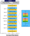 |
Fig. 1 Sketch of the main part of the SPECTROTRANSLATOR algorithm. The difference between the spectroscopic parameters of catalogue A and B (∆Xa→b) are computed in a deep fully connected network, where the inputs are composed of the spectroscopic parameters from catalogue A, and of photometric colours. The deep network of depth-n is made by a series of n blocks of progressively increasing complexity, until a central layer of maximum complexity, before decreasing symmetrically. Each block is composed of a REsNET-like unit (see Sect. 2.1), illustrated on the right part, and of a linear layer that adjust the number of feature (nf ) between each depth. Finally, the difference predicted by the deep network are added to the spectroscopic parameters of catalogue A to compute the parameters values expressed in the base of catalogue B. |
2.2 Range of application of the algorithm
Due to its conception, the SPECTROTRANSLATOR algorithm has to be trained on a subset of stars in common between two surveys, namely, the training set. However, the parameter space covered by this training set is not necessary representative of the individual parameter space covered by these two surveys. This difference between them might lead to misinterpretation when the trained algorithm is applied to the entire catalogue of the input survey, as the coverage of its parameter space is likely larger than the range of parameter space covered by the sample used to train the algorithm. Therefore, it is crucial to estimate the range of parameters in which the transformations obtained by the trained algorithm are valid.
For the SPECTROTRANSLATOR algorithm to be pertinent, it is essential to have a training sample sufficiently populated that represents well the parameter space of the union of the two surveys. This union sample does not necessarily need to be uniformly distributed across the parameter space, although this might require applying a weighting scheme to the data. However, it must adequately sample the full coverage of the parameter space.
It is noteworthy that the application domain of the SPECTROTRANSLATOR is independent of the fraction of the output survey (base B) covered by the training sample, provided the latter is sufficiently populated to encompass the full parameter space of the unions area between the input and output surveys. Indeed, as long as the latter point is correct, stars of the output survey (B) located outside the union area are beyond the scope of any stars from the input survey (base A). This means they do not have counterpart in the input survey and so, they are outside the domain of application of the SPECTROTRANSLATOR by default. It is essential to emphasise, however, that it is important to know the fraction of the output survey covered by the training sample if we intend to analyse data from the input survey (A) transformed by the SPECTROTRANSLATOR algorithm in the same way as for the output survey (B). Nevertheless, such analyses should be conducted on a case-by-case basis, and it is beyond the scope of this paper to present a universal method for performing this analysis.
On the other hand, it is crucial to know how representative is the training sample compared to the entire input catalogue (catalogue A); namely, to know the domain of the parameter space where the algorithm is reliable to transform the data from catalogue A to B. To estimate the domain of validity of the algorithm, we created a bit mask by binning the input parameter space. For the bins occupied by at least stars of the training sample, we can conclude that the transformation done by the algorithm is valid in the range covered by the bin, and their bitmask value is set to 1. For the bins that do not respect that condition, the results given by the algorithm are extrapolated, and they have to be treated carefully, as it is not possible to assert their validity in the range of parameters covered by the bin, and their bitmask values are set to 0.
Binning the data in n-dimensions, where n corresponds to the number of input parameters, can become quickly extremely costly in terms of computational memory, as the number of bins used for this task is proportional to 𝒪(Cn). For this reason, the choice has been made to bin the parameter space for each possible combination of two input parameters, rather than binning the n dimensional parameter space. This simplification comes at the cost of losing information on the correlation between more than two parameters, but has the advantage that the number of bins decreases to 𝒪(n). Thus, with this method, the validity of the transformation predicted by the algorithm for a given star is evaluated for all the possible combinations of two input parameters. In practice, for simplicity, the validity of the transformation is indicated by a boolean flag only if all the parameters are inside the parameter range of the training sample. However, the problematic set(s) of parameters are indicated in one of the columns (QFLAG_COMMENTS, see Appendix A) of the catalogue of transformed values.
In practice, in the SPECTROTRANSLATOR algorithm, the training sample defines the minimum and maximum range of validity of each parameter, as the algorithm is by definition defined between these ranges. Then, to make the different bit-masks, each parameter is decomposed in the same number of bins between these ranges. This number of bins has been set to 30 by default in the SPECTROTRANSLATOR algorithm after having tested different values using the training and validation sample of the test case presented in Section 3. However, a different value might be more suitable for different dataset, depending of the number of stars that they contain, the number of parameters or the range of these parameters. In the example shown in the next section, this leads to a resolution of the application domain where the algorithm is valid for ~110 K for the effective temperature, ~0.15 dex for the surface gravity, ~0.1 dex in metallicity, ~0.07 dex for [Mg/Fe], and ~0.05 mag for the (BP – G) and (G – RP) colours.
Following the same procedure, a series of bitmasks were constructed from all the combinations of the output parameters. As stated above, this was not done to estimate the representativity of the training sample in comparison to the entire output catalogue (catalogue B). Rather, it is meant to help flag the stars located in regions of the parameter space where the SPECTROTRANSLATOR algorithm might not be fully reliable. This is particularly the case for the stars located near the border of the domain of application in the input parameter space.
3 A test case: Transforming GALAH to APOGEE
In the following section, we present an example of an application of the SPECTROTRANSLATOR algorithm to transform the effective temperature (Teff), surface gravity (log(𝑔)), metallic-ity ([M/H]), magnesium abundance ([Mg/Fe]), and line-of-sight velocity (Vlos) from the GALAH catalogue (catalogue A) into the base of the APOGEE-2 catalogue (catalogue B). Note that we have chosen to use the individual abundance ratio [Mg/Fe] instead of the global α-abundance ratio ([α/Fe]). This decision is based on the fact that the [α/Fe] values obtained from GALAH and APOGEE-2 may reflect the abundances of different elements due to their distinct wavelength ranges. In a comparison of values measured between APOGEE and optical measurements for a set of stars in common, Jönsson et al. (2018) found that magnesium exhibits the highest accuracy among α-elements.
Therefore, in this example application of the SPECTROTRANSLATOR, we preferred to use [Mg/Fe] rather than the global [α/Fe] because it refers to the same chemical element between the two surveys and offers a more accurate scientific value for the science case presented in Sect. 4. However, it is always possible to apply the SPECTROTRANSLATOR to transform the global α-abundance ratio.
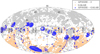 |
Fig. 2 Sky coverage (in Galactic coordinates) of the 16583 stars in common (in blue) between APOGEE-2 DR17 and GALAH DR3 that fullfil the criteria listed in Sect. 3.1, overlaid on the spatial coverage of these two surveys (in grey and orange, respectively). |
3.1 Data
3.1.1 Catalogue A: GALAH DR3
The stellar parameters and chemical abundances we applied the transformation to come from the main catalogue of the third data release of the GALAH survey (Buder et al. 2021). This catalogue contains 588 571 stars observed at high resolution (R ~ 28 000) in four non-continuous wavelength regions in the optical (between 4713 and 7887 Å) using the High Efficiency and Resolution Multi-Element Spectrograph (HERMES, Sheinis et al. 2015) mounted on the 3.9 m Anglo-Australian Telescope (AAT). The data reduction pipeline used to derive the stellar parameters of the GALAH DR3 catalogue is mostly described in Kos et al. (2017), with a few modifications listed in Buder et al. (2021). Following the best practices recommendations for GALAH DR35, and the work of Hegedus et al. (2023), we selected only the stars respecting all the following criteria:
signal-to-noise ratio (S/N> 30) (SNR_C3_IRAF> 30),
VBROAD < 15 km s−1 to remove stars with significant rotation,
have no flagged problems (FLAG_SP=0),
have valid [Fe/H] and [Mg/Fe] estimate (FLAG_FE_H=0 and FLAG_MG_FE=0),
to have a corresponding entry in the Gaia DR3 catalogue, based on the crossmatch provided by the GALAH team.
The application of these criteria lead to a GALAH DR3 sample of 293 314 stars. The input spectroscopic parameters are TEFF, LOGG, FE_H and MG_FE for the intrinsic parameters, and RV_GALAH for the extrinsic network.
3.1.2 Catalogue B: APOGEE-2 DR 17
The data used to define the base B are from the last data release (DR17) of the APOGEE-2 (Apache Point Observatory Galactic Evolution Experiment, Majewski et al. 2017; Abdurro’uf et al. 2022). It contains 733 901 stars observed at high resolution (R ~ 22 500) in near-infrared (15 140–16 940 Å) by the APOGEE spectrographs (Wilson et al. 2019) mounted on the Sloan 2.5 m telescope of the Apache Point Observatory (Gunn et al. 2006) and on the 2.5 m Irénée du Pont telescope (Bowen & Vaughan 1973) at Las Campanas Observatory. The stellar parameters and chemical abundances have been obtained within the APOGEE Stellar Parameters and Chemical Abundances Pipeline (ASPCAP, GARCÍA PÉREZ et al. 2016), from which we use TEFF, LOGG, M_H and MG_FE for the intrinsic network, and VHELIO_AVG as the output of the extrinsic network.
As previously, to compile an APOGEE-2 sample of 455 486 stars, we followed the recommendations for APOGEE DR176 and the work of Hegedus et al. (2023). Thus, we selected only the stars respecting all the following criteria:
S/N>100
are not flagged as STAR_BAD7, FE_H_BAD, and ALPHA_FE_BAD in the APOGEE_ASPCAPFLAG bitmask,
the limitation of the scatter in los velocity VSCATTER < 1 km s−1 in order to eliminate most binaries and other variable stars,
have a Gaia DR3 counter-part, with the cross-identification made by the APOGEE team.
3.2 Training setup
There are 16 583 stars in common between the selected APOGEE-2 and GALAH DR3 samples as selected in Sect. 3.1, which position is shown in Fig. 2. These stars constitute the basis for the training/validation sets. From these, we excluded all the stars located in regions of high extinction (E(B – V) > 0.3) based on the extinction map of Schlegel et al. (1998) recalibrated by Schlafly & Finkbeiner (2011), as the Gaia colour in these regions (mainly located close to the Galactic plane) might be significantly affected by the extinction. Therefore, 13, 664 stars are used to train and validate the algorithm, separated between the training set, composed of 10 931 stars (80% of this initial sample) randomly selected, and of the validation sample composed of the other 2733 stars (20%). We note here that the training set of the intrinsic network can be composed of different stars than the training set of the extrinsic network as these two networks are trained independently.
To illustrate the complex dependency of the parameter transformations from base A to B, mention in Sect. 2, we show in Fig. 3 how the difference between the metallicity (surface gravity) values from GALAH and APOGEE-2 depend on the surface temperature and of the surface gravity (metallicity) for the stars of the training and validation samples that are in common between the two surveys. This high degree of entanglement between the parameters from one base to another justified our choice to base the SPECTROTRANSLATOR on a neural network.
For the intrinsic network, the transformation from base A to В is computed from the spectroscopic parameters from GALAH XA,intr =[TEFF, LOGG, FE_H, MG_FE] and from the extinction corrected colours θintr= [(BP – G)0, (G – RP)0], where the reddening conversion coefficients are adopted from Marigo et al. (2008), following previous works (e.g. Sestito et al. 2019; Thomas & Battaglia 2022). The parameters expressed in base В (here APOGEE-2) are XB =[TEFF, LOGG, M_H and MG_FE] from APOGEE-2.
We note here that all the input and output parameters are normalised to have a distribution with a mean equal to zero and a standard deviation of one with respect to the training sample, done using the STANDARDSCALER of the SCIKIT-LEARN library (Pedregosa et al. 2011). This process is standard when using neural networks, as it increases significantly the stability of the network, and avoids the loss function8 to be dominated by one of the parameters. The values and the parameterisation of the SPECTROTRANSLATOR presented below have been optimised for the base transformation from GALAH to APOGEE-2.
This parameterisation will be used by default for other transformations that we will provide in the future, unless specified otherwise. However, the design of the SPECTROTRANSLATOR is relatively flexible, allowing for adjustments in the number of layers used, the number of neurons per layer, or the loss function employed (see below), to accommodate transformations from other bases or for a different set of parameters to transform. As shown in Fig. 1, the adopted network has a depth of 3, and reaches a maximum of 512 neurones per layer at the central layer. The loss function used here is a mean absolute error (MAE) function due to the potential high number of outliers, in particular at low metallicity where the number of stars is lower than at high metallicity; other loss functions like the mean square error are more sensitive to outliers. The parameters (weights and biases) of each neurone that minimise the loss function are computed iteratively using the adaptive moment estimation optimisation method (also known as Adam, Kingma & Ba 2014). This is a modification of the classical stochastic gradient descent method that prevents it from falling into a local minimum. The algorithm is trained with three successive learning rate hyper-parameters (10−3, 10−4, and 10−5). To limit the amount of time needed to train the algorithm, the training phase is allowed to stop before it reaches the maximum of established epochs (1000 here) if the loss value of the validation set did not improve during the last 20 epochs. In such cases, the trained parameters used correspond to the parameters found at the epoch where the loss function of the validation set reached its minimum. The reason of choosing to monitor the loss function of the validation set instead of the one of the training set was made to prevent overfitting. With these conditions, in this specific case presented here, the intrinsic network needs to be typically trained over ~900 epochs in less than 30 minutes on a 8×1.90 GHz machine, as one can see in Fig. 4.
For the extrinsic network, a similar setup is adopted, with similar input as for the intrinsic network to which the los velocity of GALAH (RV) has been added, and the output corresponds to the average l.o.s velocity of APOGEE-2 (VHELIO_AVG). In addition, we removed the binary candidates listed in the catalogues of either Price-Whelan et al. (2020) or Traven et al. (2020), on top of removing stars with a scatter between different measurement in APOGEE-2 of more than 1 km s−1. Despite these criteria, we found that some stars were having very high discrepancies between the l.o.s. velocity measurement of GALAH and APoGEE-2, which we attributed to potential binaries or other suspicious objects (e.g. pulsating stars). We therefore perform a 5-σ clipping on the difference of measurement between GALAH and APoGEE-2. This let us with a total of 12 266 stars with, 9813 (2453) stars in the training (validation) sample of the extrinsic network.
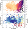 |
Fig. 3 Variation of the metallicity (upper panel) between the APOGEE and GALAH values as function of the effective temperature and colour-coded by the median surface gravity from GALAH, for the stars of the training/validation sample (see Sect. 3.1). The lower panel shows the variation of the surface gravity between the two surveys as function of the effective temperature and median metallicity values from GALAH for the same stars. |
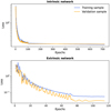 |
Fig. 4 Evolution of the loss function as a function of the epoch for the intrinsic network (on the top panel), and of the extrinsic network (on the bottom panel). The loss of the training sample is shown by the blue curve, while the one of the validation sample is shown by the orange line. |
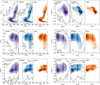 |
Fig. 5 Comparison between the coverage of the parameter space for stars in the training sample using the original GALAH data (in purple, left panels), the original APOGEE-2 data (in blue, middle panels) and the parameters transformed from the GALAH into the APOGEE-2 base by the SPECTROTRANSLATOR algorithm (in orange, right panels). The contours in the right and middle panels depict the 1, 10, and 100 stars per bin limits in the selected GALAH DR3 catalogue (refer to Section 3.1.1) and APoGEE DR17 (refer to Section 3.1.2), respectively. |
3.3 Results of the intrinsic network
3.3.1 Analysis
Fig. 5 presents a comparison of the parameter space covered by the training set using the spectroscopic values of the GALAH catalogue, XA (in purple), of the “original” APOGEE-2 catalogue XB (in blue), and of the values transformed by the SPECTROTRANSLATOR algorithm, X′B (in orange). A visual inspection of this figure shows that the coverage of parameter space for the spectroscopic parameters transformed by the algorithm is more similar to the coverage of the original APoGEE-2 values than of that of the GALAH data, confirming the strength of the algorithm to correctly transform the data from one base to another. This is particularly visible on the [Fe/H]–[Mg/Fe] diagram where the thin and thick (low and high-α) disc separation (around [Mg/Fe]~0.15) is more enhanced with the transformed values than with the initial GALAH data, comparable to the separation visible with the APoGEE-2 data. This enhancement of the thin/thick disc separation is also particularly visible in the log(𝑔)–[Mg/Fe] and Teff–[Mg/Fe] diagrams. In general, one can clearly see that the [Mg/Fe] parameter is the one which is the most affected by the change of base from GALAH to APoGEE-2, and that this change seems to be correctly learned by the algorithm. However, there is also a significant difference in the metallicity between the GALAH and the APoGEE-2 data, which seems to be correlated to the surface gravity, and in particular for the giant stars (log(𝑔) < 3.5), as they cover a wider range of metallicities in APoGEE-2 than in the GALAH at a given log(𝑔). It is interesting to see that despite that difference between the two bases, the SPECTROTRANSLATOR algorithm is able to learn the transformation and to recover the wider spread seen in APoGEE-2. The algorithm is also able to transform correctly the effective temperature and the surface gravity, as attested by the distribution of the red clump stars (around log(𝑔) ≃ 2.5) and of the metal-poor end of the top of the red giant branch (Teff ~ 5000 K and log(𝑔) < 2.3).
This qualitative analysis of the performance of the SPECTROTRANSLATOR algorithm is confirmed quantitatively by comparing Figs. 6 and 7. In Fig. 6, we show the difference between the “original” GALAH (Xa) and the APOGEE-2 (Xb) values for each parameter for the stars in the training/validation sample, while Fig. 7 shows the same relation but with the transformed (XB′) instead of the “original” GALAH value. On these figures, the black points in the left panels correspond to the residuals for the stars of the validation set, while the residuals of the training set are illustrated by the shaded bins, corresponding to 1σ, 2σ, and 3σ around the local mean of the residual. This separated analysis of the residual for the training and validation sets is important, as we can see that the trained algorithm is not subject to overfitting since the trends visible in the variation of the residuals are similar between the training and validation sets for all the parameters. Note here that we do not show the trend of the training set for the region where the number of stars per bin is lower than five due to the poor statistical information that they hold. We can see that the GALAH parameters after the transformation into the APOGEE-2 base  are well in agreement with the original APOGEE-2 values (XB), as for all the parameters, the mean of the residuals is around zero, with a scatter of
  , σ[Fe/H] = 0.065 dex and σ[Mg/Fe] = 0.050 dex, significantly lower than the scatter of the difference between the “original” GALAH and APOGEE-2 values
  , σ[Fe/H] = 0.097 dex, and σ[Mg/Fe] = 0.096 dex). Moreover, for the effective temperature, the surface gravity and the metal-licity, the residual between the transformed and the ‘original’ APOGEE-2 values do not show any trend with the value of the corresponding parameter, while the difference between the ‘original’ GALAH and APOGEE-2 values present clear trends, in particular for the giant stars with low surface gravity and for the most metal-poor stars. For the Mg abundance, we can see that for [Mg/Fe]< −0.15 dex (in the APOGEE-2 base), the transformed abundances are in average higher than in APOGEE-2 by typically 0.1 dex, while for [Mg/Fe]> 0.4 dex we observe the opposite trend. A similar trend, although twice more important, is present between the ‘original’ GALAH and APOGEE-2 values. The fact that the SPECTROTRANSLATOR is not able to completely remove this trend as it does with other parameters is likely the consequence of the low number of stars in the training sample present in these regions, 46 (0.42%) and 47 (0.42%), respectively.
The residuals that we obtained using the SPECTROTRANSLATOR are slightly larger than the residuals obtained by Nandakumar et al. (2022) who used directly the GALAH spectra and trained the CANNON-2 (Ness et al. 2015; Casey et al. 2016) algorithm to obtain the spectroscopic parameters on the APOGEE base (refer to as GCAA in their paper), except for the surface gravity. Indeed, they found a residual between the values estimated by the CANNON algorithm and the ‘original’ APOGEE values of 58 K for the effective temperature, 0.12 dex for the surface gravity, 0.04 dex for the metallicity and 0.02 dex for the [α/Fe] value. However, it is important to note here that they used the values from APOGEE-2 DR16, and their [α/Fe] parameter is the general α-abundance, composed of a combination of several elements. This might explain the differences that we have regarding the [α/Fe]–[Mg/Fe] residual.
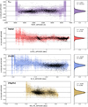 |
Fig. 6 Variation of the residuals between “original” GALAH (XA) and APOGEE-2 (XB) values for each output parameters. Left: validation set shown with black points, while the shaded areas correspond to the 1, 2, and 3σ around the local mean of the residual obtained from the training set. Bins where the number of stars in the training set is lower than five are not shown, due to the poor statistic in them. The horizontal dashed lines correspond to the average 3σ of the residuals. Right panels: the coloured histograms show the difference between the ‘original’ GALAH (XA) and APOGEE-2 (XB), and black curve shows the Gaussian fitted to this histogram used to measure the average mean and standard deviation of the residuals, which are quoted on the right panels of each parameters. |
 |
Fig. 7 Similar to Fig. 6, but with residuals between the transformed |

 |
Fig. 8 Relative importance that each feature has on the transformation of the parameters in the APOGEE-2 base, computed from the mean absolute SHAP values (see Sect. 3.3.2). |
3.3.2 Feature importance
In the previous section, we showed that the SPECTROTRANSLATOR algorithm is able to correctly learn the transformation from the GALAH to the APOGEE-2 base, but we did not explore the contribution of each parameter in this transformation.
Due to their complex non-linear nature, neural networks are in general hard to interpret, in particular regarding the importance that each input parameter (or feature) has. However, in the last years, partly motivated by the ‘right to explanations’ established by the European Union9, a lot of progress has been made in the interpretability of these systems, and feature importance ranking has become an active research area (e.g. Samek et al. 2017; Wojtas & Chen 2020). Many methods are now available to interpret the importance that each input feature has in a deep neural network (e.g. Tulio Ribeiro et al. 2016; Ribeiro et al. 2018). Among them, one of the most popular is the SHapley Additive exPlanations (SHAP, Lundberg & Lee 2017) method, which is based on the optimisation method developed by Shapley (1953) to assign the payouts of each player in cooperative game theory, known as Shapley values. In general, the Shapley values are computationally expensive to measure, as they require retraining 2n times the neural network, where n is the number of input features. The SHAP estimation method encompass a range of different techniques, including the popular LIME method (Tulio Ribeiro et al. 2016), to approximate the Shapley values while reducing significantly the computational cost. The SHAP values indicate the contribution of each input feature (XA, θ) to move the transformed values (XB′) from the mean of the prediction.
To compute the SHAP values and to estimate the importance (Imp) of each input feature, we used the KERNELEXPLAINER method from the SHAP python package10. The ‘typical’ input values of the trained SPECTROTRANSLATOR network are obtained by selecting randomly a subsample of 100 stars from the training set. These typical input values are then used to compute the individual SHAP values at the location in the parameter space of 100 stars randomly selected from the validation sample by performing 100 permutations. This results in a total of 100 × 100 × 100 computations, and take a few minutes on a 8 × 1.90 GHz machine. Then, the average relative importance (Impi,j, expressed in percentage) of an input parameter (i) in the prediction of a given output feature (j) is computed as the mean of the k = 100 individual absolute SHAP values, such as:
 (4)
(4)
We note that we can compute the relative contribution of each input feature in that way because we are working with the standardised input values (mean of zero and standard deviation of one), as otherwise, the SHAP values of the effective temperature will be largely dominant, given its larger spread in numerical values compare to the other input parameters. This also means that these values have to be interpreted with caution, as a change in the scaler method (e.g. from a standard scaler to a min-max scaler) can change the mean absolute SHAP values and so the relative importance of each input feature.
The relative importance that each feature has on the transformation from the GALAH to the APOGEE-2 base for the different spectroscopic parameters are shown in Fig. 8. Before analysing this figure, a few warnings have to be addressed for the reader to not over-interpret it, as SHAP based graphics can lead to misleading interpretation and are not always reliable, as shown by Slack et al. (2019). First, here we are showing the average relative importance of each feature for the global dataset. However, the importance of each input may depend on the location in the parameter space. For example, the effective temperature plays a less important role in the transformation of the metallicity for the metal-poor stars than for the metal rich stars (see Appendix B).
This leads to the second point, that the mean of the average SHAP values are computed using a sample of 100 randomly selected stars from the validation sample. This implies that the relative importance of each input feature is mostly indicative of the sub-sample of stars the most present in the samples, i.e. metal-rich stars ([Fe/H] > −0.5) around the main-sequence turn-off. Finally, the relative importance is given for a given number of input parameters. In other words, if we retrain the SPECTROTRANSLATOR algorithm with fewer input parameters, the precision of the transformation will not necessarily be strongly impacted. For example, in Fig. 8, the two Gaia colours provide 28% of the information to compute the output effective temperature expressed in the APOGEE-2 base. However, retraining the algorithm without the colours leads to a transformation of the effective temperature 17% less precise, as we discuss below.
As already mentioned, in the model presented here, the colours have a lot of weight in the transformation of the effective temperature, as it can penalise stars of a given effective temperature (in the GALAH base) that have Gaia colours different than the average colour of the stars at that temperature. Thus, these stars will have a higher transformation than the others, leading to a larger difference between the input and the output effective temperature. In that way, it might be better to interpret the relative importance of the input features presented in Fig. 8 as the weight that each parameter can have to penalise the transformation GALAH to APOGEE-2. Therefore, given these different caution points, Fig. 8 can and should be used only as an indicative graphics of the relative importance of each input feature.
This important caution point made, Fig. 8 shows that the transformation of the effective temperature is mostly dependent of the input effective temperature expressed in the GALAH base and of the Gaia colour, but we can see a small dependence on the other parameters, and in particular of the metallicity, as indeed, the difference between the GALAH and APOGEE-2 effective temperature is more important for metal-poor stars than for the metal rich ones (Nandakumar et al. 2022), due to smaller and less numerous absorption lines present in the former compared to the latter. Similarly, for the surface gravity transformation, the majority of the information comes from the input surface gravity from GALAH (75%), and the rest is mostly coming from the effective temperature and from the colours, which might be explained by the highest difference between the surface gravity expressed in the GALAH and APOGEE-2 at the cooler and redder end (Teff < 4500 K) of the training sample than in other region. The same reason is likely behind the relatively high importance of the temperature and colours for the transformation of the metallicity. For the [Mg/Fe] transformation, it is interesting to see that the most important information comes from the metallicity and not from the input GALAH [Mg/Fe]. However, this might be explained by the fact that at the high metallicity end, in the APOGEE-2 data, there are two [Mg/Fe] tracks clearly identified, usually attributed to the thick and the thin disc, and that at low metallicity ([Fe/H] < −1.0), there is only a single track but with a wider distribution of [Mg/Fe], and this separation is less visible with the GALAH data. Therefore, a possible interpretation is that the algorithm first uses the metallicity to have an estimation of [Mg/Fe], and then uses the input [Mg/Fe] from GALAH to refine its estimation and to break the degeneracy between the thin and thin disc track if the star is metal-rich. Moreover, the dependence on the surface gravity and the effective temperature is likely linked to the fact that 97% of the metal-poor stars in the training sample are giant stars (log(ɡ) < 3.5). Another possible explanation for the strong dependence of [Mg/Fe] on [Fe/H] is the intrinsic correlation that exists between magnesium abundance and metallicity when using the parameter [Mg/Fe] instead of [Mg/H]. To test this hypothesis, we retrained the SPECTROTRANSLATOR using [Mg/H] instead of [Mg/Fe] for both GALAH and APOGEE-2. We found that the translation of the magnesium abundances is less precise than when using [Mg/Fe] directly, with a scatter between the predicted and the “original” (recomputed) APOGEE-2 [Mg/Fe] values of 0.60 dex, compared to 0.50 dex when using [Mg/Fe] in the translation, with a similar trend in the residuals.
As already mentioned, without the Gaia colours, the transformation of the effective temperature from the GALAH to APOGEE -2 base leads to a higher scatter on the residual of ΔTeff = 89.5 K, than when the colours are used by the SPECTROTRANSLATOR (ΔTeff = 76.3 K). We note that in the former case, the input effective temperature plays a bigger role in the translation of the effective temperature. Regarding the other parameters, without colours, the scatter on the residual of the metallicity is slightly higher (Δ[Fe/H]] = 0.072 dex) than when the colours are used (Δ[Fe/H]] = 0.065 dex), but the scatter on the residual of surface gravity (Δlog(ɡ) = 0.108 dex) and of the Mg abundance (Δ[Mg/Fe]] = 0.051 dex) are very similar in both cases. However, this last point has to be nuanced, as for giant stars (log(ɡ) < 3.0 dex), the inclusion of the colours increase the precision of the surface gravity of 10% and up to 23% for the metallicity.
Intriguingly, we found that the increase in the residual of the effective temperature between the cases with and without using the colours for the translation is dependent on the signal-to-noise ratio (S/N) of the input data (SNR_C3_IRAF), as shown in Fig. 9. This clearly shows that the colours are indeed very useful in complementing the information provided by the effective temperature for the transformation from one base to another, particularly for the stars with the lowest S/N. In this figure, we can note a decrease in the residual with the S/N of the input data. A similar behaviour was observed for all the other parameters, except for the surface gravity. This shows the limitation of the current dataset used here to train the SPECTROTRANSLATOR. This indicates that for future transformations, the S/N should be used to increase the weight of stars with higher S/N when training the SPECTROTRANSLATOR. However, we reserved the analysis of the impact of weighting the training sample for a future work (see also next section).
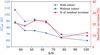 |
Fig. 9 Relation between the residuals of the transformed and the ‘original’ APOGEE-2 values for effective temperature as a function of the S/N of the input data is depicted for two cases: when colours are used for the transformation (circles) and when colours are not used (squares). The red line shows the percentage increase in the residual of the effective temperature for the transformation without colours compared to the transformation using colours. |
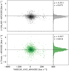 |
Fig. 10 Comparison between the difference of the l.o.s. velocity measured by GALAH and APOGEE-2 on the top panel, as well as the difference of the velocity transformed by the SPECTROTRANSLATOR algorithm and the APOGEE-2 data on the bottom panel, as a function of the l.o.s velocity measured by APOGEE-2. In both cases, the symbols show the stars of the training set. The histograms on the right panels show the distribution of the difference between the l.o.s. velocity measured by GALAH and APOGEE-2 (on top) and between the transformed GALAH l.o.s and the “original” APOGEE-2 values. |
3.4 Results of the extrinsic network
As visible on the upper panel of Fig. 10, the difference between the velocity measured by GALAH and by APOGEE-2 are in average offset by 0.3 km s−1 with a typical scatter of 0.47 km s−1. However, this velocity difference presents several inhomo-geneities, in particular around VHELIO_AVG_APOGEE = 0 km s−1 , where the difference is higher than in other regions. The offset is smaller than the one of 0.52 km s−1 measured by Tsantaki et al. (2022). This difference can be explained by the difference in the data release adopted, as Tsantaki et al. (2022) used APOGEE-2 DR16 and GALAH DR2. It can also be a consequence of the method used to compute the offset, as in Tsantaki et al. (2022), the offsets are given w.r.t Gaia-RVS, using all the stars in common between a given survey and Gaia-RVS, while in our case, we are only using the stars in common between the two surveys.
By comparing the lower to the upper panel of Fig. 10, we can see that the SPECTROTRANSLATOR algorithm is able to correct for most of this bias, but at a cost of a scatter 1.7 times larger than the original data. As such, a simpler linear correction of the bias of 0.313 km s−1 might give better results than the extrinsic network. However, this clearly shows the limitations of using an unbalanced dataset, which does not cover homogeneously the entire parameter space, when training the SPECTROTRANSLATOR. Indeed, the fact that the extrinsic network performs less well than the intrinsic one is likely a consequence of the high concentration of stars between VHELIO_AVG_APOGEE = −50 km s−1 and 50 km s−1 compared to other regions. Therefore, the relation learned by the network is largely influenced by the stars located in this region and less for the stars with different velocities. It might be possible to rebalance the influence of each star of the training sample by imposing that the relative weight on the loss function of the stars at large velocity is more important than that of the stars between VHELIO_AVG_APOGEE = −50 km s−1 and 50 km s−1, either by increasing their number with a Monte Carlo sampling, or directly by including the weights in the loss function11. However, our exploratory tests show that the criteria and the way to perform this rebalancing may strongly influence the results, and it is highly connected to how the boundaries of the parameter space of the training and validation sample are defined. As a consequence, we reserve the exploration of which method is the most suitable for a future work.
It is interesting to see that the distribution of the residuals as function of the velocity is different between the upper and lower panels, indicating that the SPECTROTRANSLATOR not only corrects from the bias in velocity, but also finds some correlation between the difference of velocity of the two surveys and some other parameters. In Fig. 11, we can see that the most important parameter in the transformation is, without surprise, the input l.o.s. velocity from GALAH, with minor contribution of the effective temperature, the colours, the surface gravity, the metallicity and the Mg abundance respectively. This is very interesting, since Tsantaki et al. (2022) found that both surveys display a common trend in metallicity for the l.o.s. velocity compared to Gaia, but only APOGEE-2 reveals a trend in temperature. However, this can be explained by the fact that we are comparing GALAH with APOGEE-2, rather than to a homogenised catalogue, as was done by the SoS. We reserve this latter comparison for future work.
3.5 GALAH transformed to APOGEE-2 catalogue
We applied the trained SPECTROTRANSLATOR algorithm to the ~590 000 stars from GALAH DR3 that have a Gaia DR3 counterpart. We note here that we did not apply any selection criteria contrary to the selection made in Sect. 3.1.1.
We trained the SPECTROTRANSLATOR five times by shuffling the training and validation sets. This set of five trained networks is used to estimate the systematic error on each of the transformed parameters caused by the method itself, and to limit the problem of overfitting. A similar method has been used by Thomas et al. (2019) to estimate the systematic error in the prediction of photometric distances. In practice, the transformed values are obtained using five different machine learnings. Then, the two extreme predictions for each transformed parameter of a given star are discarded. The value of the transformed parameters are given by the mean of the values for the three non-discarded networks, while the standard deviation is considered as the systematic error.
Another source of uncertainty on the transformed parameters is caused by the measurement uncertainties on each of the spectroscopic parameters. The probabilistic distribution function (PDF) of the transformed parameters is obtained by applying the method described above to a set of 100 Monte-Carlo resampling of the input parameters (XA, θ). In the catalogue available online12. we provide the 5, 16, 50, 84, 95-th percentiles of the PDF for each parameter. The systematic error included in the catalogue corresponds to the 50th percentile of the PDF.
Overall, 14% of the stars from the GALAH DR3 catalogue lack measurements for at least one of the input parameters, particularly [Mg/Fe]. In such cases, we set the missing ‘renor-malised’ input value to 0 and proceed with the transformation using this value. Since all input parameters of a network are normalised to have a distribution with a mean of zero and a standard deviation of one with respect to the training sample (see Sect. 3.2), setting a missing value to 0 is equivalent to assigning it the average value of the parameters in the physical (non-renormalised) space. In such instances, a flag indicating that an input was missing is raised. The provided catalogue includes a flag for both the missing input of the intrinsic and extrinsic networks.
Furthermore, for both networks, the catalogue provides quality flags that indicate if the input and output parameters are inside the range of application of the SPECTROTRANSLATOR, as we define it in Sect. 2.2. The metadata of the GALAH DR3 catalogue transformed onto the APOGEE-2 DR17 base are explained in Table A.1.
 |
Fig. 11 Relative importance of each feature in the transformation of the l.o.s. velocity from the GALAH to the APOGEE-2 base. |
Mean [Fe/H] and [Mg/Fe] derived for the 4 globular clusters studied here using the APOGEE-2, the ‘original’ GALAH, and the translated GALAH into APOGEE-2 data.
3.6 Validation with globular clusters
In this section, our focus is on validating the accuracy of transforming stellar parameters from the GALAH to the APOGEE-2 base. To achieve this, we use four globular clusters within the GALAH and APOGEE-2 footprint – NGC 104 (47 Tucanae), NGC 288, NGC 362, and NGC 6397 – each containing more than one star with a membership probability above 0.5, as determined by the criteria outlined in Vasiliev et al. (2021).
To select cluster stars, we apply the criteria detailed in Sects. 3.1.1 and 3.1.2 on the respective GALAH and APOGEE-2 catalogues. Additionally, for the GALAH dataset, we require stars to have correct input and output quality flags for the intrinsic network (QFLAG_INPUT_INTRINSIC=TRUE and QFLAG_OUTPUT_INTRINSIC=TRUE), and no missing inputs (FLAG_MISSING_INPUTS_INTRINSIC=FALSE), ensuring the use of stars with accurate translations (see Table A.1).
Table 1 presents the average and standard deviation of metal-licity and Mg-abundance obtained using GALAH, APOGEE-2, and the translated GALAH-into-APOGEE values for each cluster. As expected, the translated GALAH values align more closely with the APOGEE-2 measurements than the ‘original’ GALAH values for both metallicity and Mg-abundance. Notably, the SPECTROTRANSLATOR reduces the scatter found in the ‘original’ GALAH data for [Fe/H] and [Mg/Fe] to a value similar to the scatter measured in the APOGEE-2 sample.
Figs. 12 and 13 illustrate the relationship between [Fe/H] and [Mg/Fe] with Teff and log(ɡ). The disparity in the average metallicity measured with APOGEE-2 and the translated GALAH data, indicated by the horizontal lines, is attributed to the generally broader coverage in effective temperature and surface gravity of the APOGEE-2 sample. However, in the regions where both surveys overlap, the translated [Fe/H] values are closer to the APOGEE-2 values than the ‘original’ GALAH values, particularly for NGC 288 and NGC 6397.
For NGC 362, the translated [Mg/Fe] values exceed those measured by APOGEE-2 in the same temperature and surface gravity range as the GALAH sample, yet they remain consistent within 1σ. This is intriguing, considering that the ‘original’ GALAH measurements, on average, align more closely with APOGEE-2 values but exhibit a wider scatter. Six stars are in common between the APOGEE-2 and GALAH samples, and are therefore part of the training/validation samples). We show on Fig. 14 [Mg/Fe] values measured by GALAH and APOGEE-2 for these six stars and we compared their location with stars from the training in the same range of temperature (4300 < Teff < 5000 K), surface gravity (1.2 < log g < 2.3 dex) and metallicity (–1.3 < [Fe/H] < –1.8 dex). It is clear that four out of the six stars are located in the region where the SPECTROTRANSLATOR overestimates the values of [Mg/Fe] compared to APOGEE-2. This discrepancy arises because these stars deviate from the GALAH-APOGEE-2 [Mg/Fe] trends observed in other stars within similar temperature, surface gravity, and metallic-ity ranges. Specifically, the APOGEE-2 [Mg/Fe] for these stars is lower (by approximately –0.13 dex) than the general trend derived from stars with the same GALAH [Mg/Fe] measurement. It is however, not clear why the [Mg/Fe] values measured by GALAH and APOGEE-2 in this cluster is different than for the other stars located in the same parameter space region. In particular, it is interesting to note that for NGC 288, which has similar properties to NGC 362, the translated values of [Mg/Fe] are closer to the values from APOGEE-2, showing that the stars of this cluster are similar to the general trend. Nevertheless, globular clusters are very complex environments, with many of them having multiple populations (e.g. Bastian & Lardo 2018; Gratton et al. 2019; Mészáros et al. 2020). For instance, it has been observed that a correlation exist between Mg and Al in many clusters (Bastian & Lardo 2018; Gratton et al. 2019, and references within), although this correlation is not systematic, especially in clusters rich in metals (Pancino et al. 2017), as are NGC 288 and NGC 362.
We did not include NGC 5139 (ω-Cen) in this analysis because it has a metallicity scatter more than two times as high as other clusters (Mészáros et al. 2020, 2021). In addition, it is offers much less information on the performance of the SPECTROTRANSLATOR than the other clusters. Nevertheless, it is worth mentioning that for the stars of this cluster observed by GALAH and APOGEE-2, we found that the SPECTROTRANSLATOR tends to change the average [Fe/H] measured with the GALAH values from −1.54 dex to −1.62 dex and the average [Mg/Fe] from 0.16 dex to 0.26 dex. As a result, these values are closer to the average measurement using the APOGEE-2 values of [Fe/H]= −1.62 dex and [Mg/Fe] = 0.27 dex, respectively.
It would be interesting to study the performance of the SPECTROTRANSLATOR when the stars belonging to globular clusters are excluded from the training sample. In the current sample, 205 stars belong to globular clusters, the majority (62%) from NGC 5139 (ω-Cen) and from (23%) NGC 104 (47 Tucanae). We will explore this, along with the effect of applying a weighting scheme to the training sample, in a dedicated paper in the future. In summary, with the exception of the [Mg/Fe] measurement in NGC 362, the [Fe/H] and [Mg/Fe] obtained by the SPECTROTRANSLATOR are closer to the APOGEE-2 measurements and exhibit lower scatter compared to the ‘original’ GALAH values. This aligns with expectations for globular clusters (e.g. Masseron et al. 2019; Mészáros et al. 2020), which only shows small scatter in metallicity.
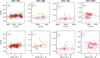 |
Fig. 12 [Fe/H] as function of the effective temperature (top row) and surface gravity (lower row) for 4 globular clusters. The parameters from the “original” GALAH data are shown by the orange points, while the value transformed on the APOGEE-2 base by the SPECTROTRANSLATOR are shown by the blue circles. The red points show the values for the stars present in the APOGEE-2 DR17 dataset. The filled circles highlight the stars observed by both APOGEE-2 and GALAH, while the open circles show the stars that have been observed either by APOGEE-2 or GALAH. The colourised triangles with the error bars indicate the average uncertainties on the individual [Fe/H] measurements in the corresponding catalogue. The horizontal red and blue lines indicates the mean metallicity of the cluster measured using the ‘original’ APOGEE-2 and transformed GALAH values, respectively. |
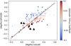 |
Fig. 14 [Mg/Fe] values measured by APOGEE-2 and GALAH for the six stars of NGC 362 observed by both surveys (in black triangle). The points show the distribution of stars from the training/validation sample in the same range of temperature, surface gravity and metallicity than the stars of NGC 362. They are colour coded by the difference between the [Mg/Fe] transformed by the SPECTROTRANSLATOR and the ‘original’ APOGEE-2. The dashed line shows the 1:1 relation in the [Mg/Fe] measurement between APOGEE-2 and GALAH. |
4 2D distribution of [Fe/H] and [Mg/Fe] in the Milky Way
In this section, we showcase the scientific utility of homogeni-sation on a common base facilitated by the SPECTROTRANSLATOR. Our focus is on exploring the insights gained by merging transformed GALAH data with APOGEE-2 data, particularly to address data gaps in regions not covered by the latter.
The combined catalogue consists of stars from both surveys, selected based on the criteria outlined in Sects. 3.1.1 and 3.1.2. As described in the previous section, we ensured the use of stars with accurately translated parameters from the GALAH sample by retaining only those with good input and output quality flags for the intrinsic network, and with no missing inputs (QFLAG_INPUT_INTRINSIC=TRUE, QFLAG_OUTPUT_INTRINSIC=TRUE, and FLAG_MISSING_ INPUTS_INTRINSIC=FALSE). For stars observed by both surveys, we preserved the original spectroscopic values from the APOGEE-2 data. To further use data with good precision on the translation, we only kept the stars from the translated GALAH dataset with systematic error on the metallicity of M_H_PRED_ERR< 0.1 dex and on the magnesium abundance of MG_FE_PRED_ERR< 0.05 dex. For both the APOGEE-2 and the translated GALAH datasets, we also only kept stars with uncertainties on the metallicity and magnesium abundance of d[M/H] < 0.2 dex and d[Mg/Fe] < 0.1 dex13. Because we did not find significant differences in the predicted and original parameters between regions of high and low extinction, we did not apply an extinction cut to make the selection, allowing us to access regions close to the Galactic mid-plane.
We note that, to ensure reliability, we discarded all stars with non-null STARHORSE_OUTPUTFLAGS and remove those within 5 half-light radii and within ±0.5 kpc from any globular clusters, following the parameters listed in Harris (1996, 2010). Finally, the stars listed as member of a globular cluster or stellar stream in the APOGEE-2 catalogue and in the catalogue of Schiavon et al. (2024) were also removed. The resulting merged catalogue comprises 571 696 stars, with 56% from APOGEE-2 and 44% from GALAH.
The Cartesian galactocentric coordinates are computed with the ASTROPY SKYCOORD package (Astropy Collaboration 2018) using the STARHORSE heliocentric distances from Queiroz et al. (2023). In this galactocentric frame, the Sun is located at [X⊙, Y⊙, Z⊙] = [−8.122 kpc, 0.0 kpc, 20.8 pc].
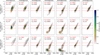 |
Fig. 15 Kiel diagram for different ranges of Galactocentric radii and vertical elevations from the midplane. The 2D histogram shows the relative distribution (made with a kernel density estimator) of the transformed GALAH data in each spatial bin. The grey iso-density contours are plotted at the 1, 5, 10, 30, 50, and 70% of the maximum density for the stars from APOGEE-2. In each bin, NG and NA refer to the number of stars from the GALAH and APOGEE catalogues, respectively. The horizontal dashed red lines show the upper and lower limit for the selection of giant stars used in Sect. 4. |
4.1 Distribution of [Fe/H] versus [Mg/Fe] across the Galaxy
We aim in this section to take advantage of the statistical and spatial increase allowed by combining together the translated GALAH and the APOGEE-2 data to study the distribution of [Mg/Fe] versus [Fe/H] at different Galactocentric radii (R) and vertical elevations from the midplane (Z), in a similar way than Hayden et al. (2015) and Queiroz et al. (2020). However, the mix of stellar type observed by APOGEE-2 and GALAH change drastically across the Galaxy, but also between the two surveys for a given R and Z. This is visible in Fig. 1514, where is presented the Kiel diagrams of the stars from the transformed GALAH catalogue, and from the APOGEE-2 catalogue at different Galactocentric cylindrical radii (R) and vertical elevations from the midplane (Z).
Therefore, to avoid having artificial variations in the [Mg/Fe] versus [Fe/H] distribution reflecting the underlying variation in the mix of stellar types observed by the two surveys, we decided to restrict our study using only giant stars in the range of surface gravity 2.5 > log(ɡ) > 1.5 dex, as indicated by the two red lines in Fig. 15, as they are present at all distances and in both APOGEE-2 and the transformed GALAH samples. This leads to a selection of 155,885 giant stars from the combined APOGEE-2 and transformed GALAH sample (66% from APOGEE and 34% from GALAH).
The close match in the distributions on the [Mg/Fe] vs [Fe/H] plane visible in Fig. 16 demonstrates the effective performance of the SPECTROTRANSLATOR in homogenising stars that are not necessarily common between two different datasets.
A similar analysis, specifically focussing on the stars in common between the two surveys, and not limited only to giant stars, is presented in Appendix C. There we demonstrate the very good agreement between the distribution of parameters when using the translated GALAH data compared to the distribution obtained using the APOGEE-2 data, which is not the case when using the ‘original’ GALAH data. This demonstrates the importance of a tool such as SPECTROTRANSLATOR to homogenise data onto the same base. Despite the close match in the [Mg/Fe] versus [Fe/H] determination at different positions in the Galaxy (in Fig. 16), subtle differences become apparent upon closer examination. For instance, in the 0 < R[kpc] < 2 and 0.5 < |Z|[kpc] < 1.0 bin, the chemically defined thin disc (low-Mg blob) visible in the APOGEE-2 data is significantly less visible in the GALAH data. This discrepancy between the two datasets can be attributed to the statistical fluctuations due to the low number of star from the GALAH dataset in that region. Nonetheless, it is interesting to see that the bimodal [α/Fe] distribution (which include Mg) observed by APOGEE in the centre of the Milky Way (Rojas-Arriagada et al. 2019; Queiroz et al. 2020) is also visible with the translated GALAH data. However, contrary to these works, a first visual inspection of that region seems to indicate that there is only a single trend which relates the low-Mg to the high-Mg overdensities, i.e. that there is not a degeneracy of [Mg/Fe] for a given [Fe/H]. This is in line with the observation of Hayden et al. (2015); Kordopatis et al. (2015b); Bensby et al. (2017); Zasowski et al. (2019); Lian et al. (2020, 2021); Katz et al. (2021); Imig et al. (2023). These differences observed between various studies using the same data are explained by Katz et al. (2021), who show that the double sequence is only visible for a couple of elements (including the global [α/M] used by Queiroz et al. 2020), while for the others (including [Mg/Fe]) they present a single trend (see their Appendix F). Note that the gap visible in the distribution of the transformed GALAH parameters around [Fe/H]~ − 1.0 in the 12 < R < 14 kpc 1.0 < |Z| < 2.0 kpc bin is the combined consequence of the low number of GALAH stars in that bin, and of kernel density estimator method used to make these plots.
Another notable difference is that the high-[Mg/Fe] plateau reaches lower [Mg/Fe] values for the translated GALAH sample compared to the APOGEE-2 sample. This discrepancy stems from the lower accuracy of the SPECTROTRANSLATOR at high-[Mg/Fe] values, as explained in Section 3.3.1. Furthermore, one can also observe that knee in the [Mg/Fe] versus [Fe/H] distribution generally appears at lower [Fe/H] in the GALAH sample than in APOGEE-2, although this is not always the case (i.e. in the 6 < R < 8 kpc, 0.5 < |Z| < 1.0 kpc bin). In the bins affected by this discrepancy, we can observe that the distribution of the two surveys on the Kiel diagram is quite different, even for the giant sample used here, with the APOGEE-2 sample reaching lower temperatures than GALAH for a given log(ɡ). On the contrary, in the bins where the discrepancy is not visible, we can see that the distributions on the Kiel diagram are similar in the surface gravity range we selected. This might suggest that the difference of location of the knee between APOGEE-2 and the transformed GALAH data is the consequence of the intrinsic selection function of the two surveys. Note here that these discrepancies are anyway significantly smaller than those that appear when using the ‘original’ GALAH values.
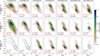 |
Fig. 16 [Mg/Fe] versus [Fe/H] distribution of the selected giant stars 2.5 > log(ɡ) > 1.5 dex in the same spatial bins as for Fig. 15. |
4.2 [Fe/H] and [Mg/Fe] cartography of the Milky Way disc
Figure 17 shows the edge-on of median [Fe/H] and [Mg/Fe] across the disc for the 155 885 selected giants, using the APOGEE-2 sample only (left) and combined with the trans-formed GALAH sample (right). The contribution of the GALAH dataset in complementing the APOGEE-2 one is clearly visible on the upper panels of the figure. We can see that not only do the GALAH data significantly increase the number of stars observed near the midplane of the disc and at different azimuth, but they also include observing areas that are not at all observed by APOGEE-2, in particular toward the Galactic centre in the Southern Galactic hemisphere (R > −8 kpc and Z < 0 kpc). This allows us to expand the [Fe/H] and [Mg/Fe] maps, and to reduce the fluctuations caused by low number statistics, particularly visible when comparing the APOGEE-2 only and APOGEE-2+GALAH [Fe/H] maps near the Galactic plane on Fig. 17. It is interesting to notice that the global distribution of [Fe/H] and [Mg/Fe] in Fig. 17 is not drastically different when using only the APOGEE-2 data or combined with the transformed GALAH data, and that the area without APOGEE data (highlighted in grey in the upper left panel) does not mark a discontinuity with the rest of the map. This highlights the efficiency of SPECTROTRANSLATOR in transforming the spectroscopic values from one base to another.
A qualitative inspection of the edge-on median metallicity map (middle panels of Fig. 17) reveals a clear radial and vertical metallicity gradient in the disc, with higher average metallici-ties near the Galactic centre and closer to the midplane, which decline towards outer radii and higher elevations. In contrast, the median [Mg/Fe] (lower panels of Fig. 17) is lower near the Galactic midplane and rapidly increases towards higher elevations, marking the transition between the thin and thick discs. The flaring of the thin disc (low [Mg/Fe]) beyond a radius of 6 kpc is clearly visible in the [Mg/Fe] map. Overall, these maps closely resemble the cartography recently produced by Gaia Collaboration (2023) and Imig et al. (2023) using Gaia and APOGEE-2 DR17 data, respectively.
4.3 Radial and vertical gradients
Here, we investigate the overall radial and vertical gradients of [Fe/H] and [Mg/Fe] across the Galaxy. First, we compare the profiles found using only the APOGEE-2 to the profiles found when APOGEE-2 data are combined to the ‘original’ or to the translated GALAH data. We then analyse these last profiles more specifically and comparing them to those found in the literature.
We divided the 155 885 selected giants into five ranges of vertical elevation on either side of the disc midplane. For each slice, we computed the running median [Fe/H] and [Mg/Fe] as a function of radius in bins 0.5 kpc with a 50% overlap between each bin. Following the method used by Martig et al. (2016), the uncertainty on the median value in each bin is estimated by measuring the median for 1000 bootstrap realisations of the sample. The uncertainties correspond to the 16th and 84th percentiles of this distribution.
Fig. 18 illustrates the median metallicity (left panel) and [Mg/Fe] (right panel) radial trends for five different elevations above (solid lines) and below (dashed lines) the Galactic mid-plane using only the APOGEE-2 data (upper panels), combining them to the “original” GALAH data (middle panels), and combined to the translated GALAH data (lower panels). Fig. 19 presents the vertical gradient of the median metallicity and [Mg/Fe] for different Galactic radii for the same three datasets. We note that in both figures, we only show bins containing at least 20 stars. These two figures show that incorporating either the “original” or the translated GALAH data into the APOGEE-2 dataset does not significantly alter the overall radial or vertical profiles. This is expected, as Fig. 17 shows that APOGEE data are the most numerous across the majority of the Galaxy. However, we can see that the GALAH data complement the APOGEE-2 data in certain regions, such as 4 < R < 6 kpc and particularly for Z < −2.5 kpc, where there is no APOGEE-2 data. The dominance of the APOGEE-2 data in most regions explains why the profiles determined using either the ‘original’ or translated GALAH data are relatively similar. Notably, in regions where GALAH data are more numerous than APOGEE-2 data, the profiles using the translated GALAH data are more similar to the profiles found using only APOGEE-2 data than those using the ‘original’ GALAH data. This is particularly evident in Fig. 18 for 0.1 < |Z| < 0.25 kpc, where we observe a local drop in the radial profile of the metallicity between 6 < R < l0 kpc that is not present in the profile using only APOGEE-2 data or when combined with the translated data. Additionally, the transition from high-Mg ([Mg/Fe] ~ 0.25) to low-Mg ([Mg/Fe] ~ 0.1) for 0.5 < |Z| < 1.0 kpc is less gradual in the APOGEE and “original” GALAH profile than in the profile using APOGEE-2 data alone or combined with the translated data. Similarly, a local peak of [Mg/Fe] near R ≃ 6 kpc between −0.5 < |Z| < −0.25 kpc, seen when combining the ‘original’ GALAH and APOGEE-2 data, is not present when using only APOGEE-2 data and is strongly reduced when combining APOGEE-2 data with the translated GALAH data. This is also visible in Fig. 19, where the vertical [Mg/Fe] profile at 4 < R < 6 kpc shows a strong local variation at Z < −3.2 kpc with the ‘original’ GALAH data, which is not present with the translated GALAH data, presenting a flatter profile more similar to the upper part of the Galactic disc in the same region. In the example presented here, the inclusion of the GALAH data only increases precision in a few regions of the Galaxy. However, it demonstrates the need for a tool like the SPECTROTRANSLATOR that can calibrate two different datasets on the same scale, as the absence of such a tool may lead to the appearance of artificial features. In the near future, the complementarity of two different datasets, will be strengthened compared to the test case shown here, in particular with the arrival of WEAVE and 4-MOST, that will have relatively similar selection function and depth, but covering different areas of the sky.
If we focus on the profiles combining the APOGEE-2 and the translated GALAH data, we observe that both metallicity and [Mg/Fe] trends exhibit similar behaviours on either side of the Galactic plane, irrespective of the elevation. A similar observation has been made by Gaia Collaboration (2023) on the Gaia data. At most elevations, we observe a break in the metallicity trend around 6–8 kpc at |ɀ| > 0.25 kpc, consistent with previous studies using different catalogues (e.g. Haywood et al. 2019; Kordopatis et al. 2020; Katz et al. 2021; Gaia Collaboration 2023). However, the radius of the break seems to vary with elevation, occurring farther out at higher elevations compared to near the plane of the disc. For regions near the Galactic midplane, no clear break is evident due to limited coverage, though a tentative plateau beginning around R = 5 kpc is discernible. This pattern aligns with findings by Imig et al. (2023) when considering both the thin and thick disc populations. Notably, the [Fe/H] value of the plateau differs from that found by Gaia Collaboration (2023) ([Fe/H] = 0.0 dex versus 0.2 dex here), but the median metallicity converges toward [Fe/H] ≃ −0.4 dex at large radial distances, consistent with various studies (e.g. Eilers et al. 2022; Imig et al. 2023) including Gaia Collaboration (2023). The absence of the ~0.5 kpc wide wiggles found by Gaia Collaboration (2023) for |Z| < 0.5 kpc and R ~ 8.5 kpc on both sides of the disc, which they partially attributed to the presence of hot turn-off stars in their sample, suggests that these wiggles may be consequences of their geometric selection biases rather than dynamical effects.
Regarding the [Mg/Fe] trends, they differ significantly from the [α/Fe] trends found by Gaia Collaboration (2023). For instance, we do not observe a clear break with a transition from a negative to a positive trend around 6 kpc for the region near the Galactic midplane. Instead, we find a clear drop in the median [Mg/Fe] value in the highest elevation bin from [Mg/Fe] = 0.3 dex to [Mg/Fe] = 0.15 dex at 8 kpc, while Gaia Collaboration (2023) found that [α/Fe] declines smoothly. These differences are explained by the dominance of calcium in their [α/Fe] abundances, which has a less extended distribution than magnesium, and because calcium is a weaker indicator of the ratio of super-novae type II over type Ia, and thus of the separation between the chemically selected thin and thick discs (e.g. Minchev et al. 2012a,b). Furthermore, we are using data with higher spectro-scopic resolution than Gaia-RVS, which contributes to explaining these differences. A less significant drop is also visible at 0.5 < |Z| < 1.0 kpc, with a decrease from [Mg/Fe] = 0.2 dex to [Mg/Fe] = 0.1 dex around 6 < R < 8 kpc. These trends resemble those found by Martig et al. (2016) and are consequences of the flaring of the thin (low-[Mg/Fe]) disc beyond ~6 kpc. This flaring is likely caused by the radial migration of thin disc stars (e.g. Minchev et al. 2012a, 2015; Kordopatis et al. 2015a). For instance, Minchev et al. (2012a), show that migrator stars increase the velocity dispersion, and so the scale-height, of the disc outside the corotation radius of the Galactic bar. Assuming a flat rotation speed of 233 km s−1 (Põder et al. 2023) and a bar pattern speed of ~eq40 km s−1 kpc−1 (Wegg et al. 2015; Sormani et al. 2015; Li et al. 2016; Portail et al. 2017; Sanders et al. 2019; Clarke et al. 2019), the corotation radius of the Milky Way with the bar is located at 5.8 kpc. Therefore, if the migrated stars come from the thin (low-[Mg/Fe]) disc, we therefore expect to observe an increase of it beyond ~5.8 kpc. This aligns with the qualitative observations seen in Figs. 17 and 18, where we observe first a slow decrease in median [Mg/Fe] with radius above |Z| = 0.5 kpc between ~ 6 and 8 kpc, followed by a rapid drop beyond.
Regarding the vertical gradient of the median metallicity and [Mg/Fe] for different Galactic radii, both the [Fe/H] and [Mg/Fe] distributions exhibit stronger vertical gradients near the Galactic midplane compared to Gaia Collaboration (2023). This difference partly stems from the radii used between both studies, as well as differences in [Fe/H] and [Mg/Fe] values between Gaia and APOGEE-2. For both [Fe/H] and [Mg/Fe], the vertical gradient is stronger near the Galactic centre than at large radii. We observe a smoother transition between the low and high [Mg/Fe] disc at larger radii, with the median [Mg/Fe] decreasing with radius at a given elevation, for |Z| > 0.5 kpc, particularly beyond ~8 kpc. This is a consequence of the flaring of the thin (low-[Mg/Fe]) disc at large distances, as visible in Fig. 17. For the metallicity, the median value evolves gradually with radius inside |Z| < 1.0 kpc. For higher elevations, the evolution of metallicity becomes similar at every radius, except in the inner Galaxy where the median metallicity is lower than at other radii at a given elevation, although it exhibits a similar gradient. Notably, the vertical distribution of the median [Fe/H] is skewed toward positive elevations at large radii, in particular in the outermost radii studied (12 < R < 14 kpc). This shift is also visible in the metallicity map of Fig. 17. The vertical shift toward positive vertical elevation at large distances is also present in the [Mg/Fe] distribution, although it is less significant than in the metallicity distribution. We note here that this asymmetry is not an artifact created by the SPECTROTRANSLATOR, as it is also visible in the APOGEE-2 data (see Fig. 19).
The observed asymmetry in the median [Fe/H] and [Mg/Fe] distributions is challenging to explain solely by the radial migration of stars, as to our knowledge, the radial migration should increase the scale height symmetrically on both sides of the disc (e.g. Sellwood & Binney 2002; Minchev et al. 2012a,b, 2013, 2014, 2015, 2017; Johnson et al. 2021). Instead, it is likely the consequence of perturbations generated by a satellite galaxy passing through the disc, as proposed by (Ibata & Razoumov 1998; Velazquez & White 1999; Kazantzidis et al. 2008; Villalo-bos & Helmi 2008; Purcell et al. 2010; Gómez et al. 2016). More recently, Laporte et al. (2018a,b) demonstrated that a coupling between the passage of the Sagittarius dwarf and the dark matter wakes generated by the infall of the Large Magellanic Cloud can induce a vertical asymmetry of density along the midplane of the Galactic disc at large Galactocentric radii. This scenario has been proposed to explain various phenomena such as the high vertical flaring observed in the outer edge of the Milky Way (Thomas et al. 2019), the formation of the Monoceros-Anticentre stream (Laporte et al. 2020a), and the presence of phase-space spiral structure in the Solar vicinity (Antoja et al. 2018; Laporte et al. 2020b). Furthermore, Ruiz-Lara et al. (2020) demonstrated that the three narrow episodes of enhanced star formation in the Milky Way during the last 6 Gyr coincide with the pericentre passages of the Sagittarius dwarf galaxy. Nevertheless, to confirm this scenario, a proper chemo-dynamical analysis is needed (e.g. Binney & Vasiliev 2023, 2024), but this is beyond the scope of this paper.
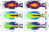 |
Fig. 17 Edge-on view of the global maps of the Milky Way, showing the number of stars observed (upper panels), the median [Fe/H] (middle panels) and median [Mg/Fe] (lower panels) distribution for the APOGEE-2 sample only (left), and combined to the transformed GALAH data (right side) in 0.2 kpc × 0.2 kpc bins. On the upper left panel, the grey area illustrates the region not covered at all by the APOGEE-2 survey, but that has been observed by the GALAH survey. In each panel, the dashed black line shows the Galactic mid-plane, and the yellow circle indicates the location of the Sun. We note that R preserve the sign of the X-axis to show the opposite side of the Galaxy. |
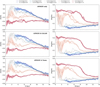 |
Fig. 18 Radial gradients of the metallicity (left) and [Mg/Fe] (right) for different elevations from the Galactic midplane. The upper row shows the profile using only the APOGEE-2 data, the middle row combining them with the ‘original’ GALAH values, and the lower row combining the APOGEE-2 data with the translated GALAH data. The trends are computed as running medians in bins of 0.5 kpc, with a 50 percent overlap, provided that at least 20 stars are available to compute the median. The shaded areas represent the uncertainty on the median (obtained from the 16th and 84th percentile of 1000 bootstrap samples). The continuous lines show the trend above the Galactic midplane (Z > 0), and the dashed lines the trend below the midplane (Z < 0). |
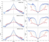 |
Fig. 19 Vertical gradients of the metallicity (left panel) and [Mg/Fe] (right panel) for different radial distance from the Galactic centre. The upper row shows the profile using only the APOGEE-2 data, the middle row combining them with the ‘original’ GALAH values, and the lower row combining the APOGEE-2 data with the translated GALAH data. The trends are computed as running medians in bins of 0.2 kpc, with a 50% overlap, provided that at least 20 stars are available to compute the median. The shaded areas represent the uncertainty on the median (obtained from the 16th and 84th percentile of 1000 bootstrap samples). |
5 Conclusions
In modern Galactic astronomy, stellar spectroscopy plays a pivotal role in complementing large photometric and astrometric surveys. By providing crucial data on stellar parameters, chemical compositions, and radial velocities, it enables deeper insights into the chemical evolution and chemo-dynamical mechanisms of the Milky Way and its satellites. Despite the wealth of existing and incoming spectroscopic data, the use of different instruments and dedicated pipelines by the various spectroscopic surveys leads to systematic differences in the derived spectroscopic parameters, which ultimately limit the scientific legacy of these data. Consequently, efforts to homogenise spectroscopic surveys onto a common scale are essential to maximise the scientific value of these data.
In this paper, we present the SPECTROTRANSLATOR, a new data-driven algorithm that is able to transform spectroscopic parameters from the base of one catalogue to that of another catalogue. This algorithm is composed of two deep-residual networks, an intrinsic and an extrinsic network. In the former, all input parameters play a role in computing the transformation of the spectroscopic parameters from one base to another. This is mostly used to compute the transformation of fundamental stellar parameters, such as the effective temperature, surface gravity, metallicity, or α-abundance. In the second, the transformation of only one of the parameters depends on all the other parameters, but this parameter does not affect the transformation of the others, perfectly adapted to compute the transformation of line-of-sight velocity or of individual abundances of some chemical elements. We demonstrated the ability of SPECTROTRANSLATOR by transforming the effective temperature, surface gravity, metallicity, and [Mg/Fe] of the GALAH DR3 catalogue to the APOGEE-2 DR17 base using the intrinsic network with very high precision, similar to the results obtained by Nandakumar et al. (2022) using Cannon directly on the spectra. Using a method to measure the importance of each parameter in the transformation, we find, for example, that the metallicity transformation from GALAH to APOGEE-2 is strongly dependent on the effective temperature and surface gravity. Furthermore, the most important parameter for the transformation of [Mg/Fe] between the two surveys is the metallicity. We also transformed the line-of-sight velocity using the extrinsic network, although in that case, the algorithm is able to correct most of the biases existing between the two surveys, but it increases the scatter. This shows the limitation in the training of the algorithm that might need to rebalance the weights of each star to find a proper relation between the two surveys. We plan to explore the impact of different rebalance strategy in a future work.
We have also presented the scientific potential of this algorithm by measuring the distribution of [Fe/H] and [Mg/Fe] across our Galaxy. Unsurprisingly, we recovered the radial and vertical [Fe/H] and [Mg/Fe] gradient and the low and high-[Mg/Fe] bimodality found in past studies (e.g. Hayden et al. 2015; Haywood et al. 2018; Rojas-Arriagada et al. 2019; Kordopatis et al. 2020; Queiroz et al. 2020; Gaia Collaboration 2023; Imig et al. 2023; Guiglion et al. 2024). However, contrary to many previous studies using the APOGEE-2 data, we found that the inner Galaxy present a single trend between the high-[Mg/Fe] and low-[Mg/Fe] region, which is explained by the fact that we are using [Mg/Fe] and not the global [α/M] (Katz et al. 2021). Interestingly, we also found that the distribution of [Fe/H] and [Mg/Fe] across the midplane of the MW is asymmetric at large radius, with the northern Galactic hemisphere more metal-rich and [Mg/Fe]-poor compared to the southern hemisphere at the same elevation. We propose that this asymmetry is a consequence of the perturbations of the outer disc generated by the passage of the Sagittarius dwarf galaxy and/or of the dark matter wakes generated by the infall of the Large Magellanic Cloud.
The transformed GALAH to APOGEE-2 catalogue presented here, the inverse transformation (APOGEE-2 to GALAH), as well as the training and validation samples used to train SPECTROTRANSLATOR in both cases, are available on our website15. We aim to update this website regularly by including the transformation of more spectroscopic catalogues, such as SEGUE (Yanny et al. 2009), LAMOST (Zhao et al. 2012), Gaia-ESO (Randich et al. 2022), DESI (Flaugher & Bebek 2014; Cooper et al. 2023), Gaia (Recio-Blanco et al. 2023), or H3 (Conroy et al. 2021). We also aim to use this methodology to homogenise spectroscopic parameters, including those from the next generation of large spectroscopic surveys, such as WEAVE (Dalton et al. 2012; Jin et al. 2024) and 4-M0ST (de Jong et al. 2010) surveys. These two surveys are complementary one to another, as WEAVE will observe the northern sky, while 4-MOST will observe the southern sky. Apply the SPECTROTRANSLATOR to these data to homogenise them on the same base will thus allow access to the entire volume of our Galaxy. However, on top of the crucial effort of homogenising datasets into the same scale, which involve tools such as the SPECTROTRANSLATOR, the study of the physical properties of our Galaxy require us to properly estimate and to take into account the different selection function of each survey.
The SPECTROTRANSLATOR algorithm promises to play a crucial role in standardising various spectroscopic surveys onto a unified basis. This capability is particularly significant given the different spatial coverage of the different large spectroscopic surveys currently underway. By providing a mean to seamlessly translate spectroscopic parameters across different observational bases, the SPECTROTRANSLATOR algorithm facilitates comparative analyses that leverage data from multiple sources. In doing so, it contributes to increasing the legacy of large surveys and in their scientific exploitation and it is poised to become an indispensable tool to unravel the complexities of our Galactic environment and beyond.
Several updates of the SPECTROTRANSLATOR algorithm are already underway, either by weighting the stars of the training sample to decrease the high heterogeneous distribution of stars across the parameter space or by transforming the architecture of the network to use a Bayesian Neural Network to take in consideration the uncertainties and possible degeneracy between the input and output features. We strongly encourage researchers to download (see details below) and to experiment with the SPECTROTRANSLATOR algorithm and to collaborate with the authors to improve it.
Data availability
A copy of the translated catalogues are available at the cDS via anonymous ftp to cdsarc.cds.unistra.fr (130.79.128.5) or via https://cdsarc.cds.unistra.fr/viz-bin/cat/J/A+A/690/A54
The SPECTROTRANSLATOR algorithm is publicly available on GitHub https://github.com/GFThomas/SpectroTranslator.git. The training/validation samples as well as the translated catalogues for different surveys is available on https://research.iac.es/proyecto/spectrotranslator/.
Acknowledgements
The authors want to thank Anna Queiroz for her help on using the Starhorse distances and for her useful suggestions. We also want to thank the anonymous referee for his comment and suggestions that help improving the strength and the clarity of the paper. G. Thomas, G. Battaglia, E. Fernández-Alvar and C. Gallart acknowledge support from the Agencia Estatal de Investigación del Ministerio de Ciencia en Innovación (AEI-MICIN) and the European Regional Development Fund (ERDF) under grant number PID2020-118778GB-I00/10.13039/501100011033 and the AEI under grant number CEX2019-000920-S. E.F.A acknowledges the HORIZON TMA MSCA Postdoctoral Fellowships Project TEMPOS, number 101066193, call H0RIZ0N-MSCA-2021-PF-01, by the European Research Executive Agency. This project has received funding from the European Research Council (ERC) under the European Union’s Horizon Europe programme “StarDance: the non-canonical evolution of stars in clusters” (ERC-2022-AdG, Grant Agreement 101093572, PI: E. Pancino). F.G. gratefully acknowledge support from the French National Research Agency (ANR) funded project “MWDisc” (ANR-20-CE31-0004) and “Pristine” (ANR-18-CE31-0017). This work has made use of data from the European Space Agency (ESA) mission Gaia (https://www.cosmos.esa.int/gaia), processed by the Gaia Data Processing and Analysis Consortium (DPAC, https://www.cosmos.esa.int/web/gaia/dpac/consortium). Funding for the DPAC has been provided by national institutions, in particular the institutions participating in the Gaia Multilateral Agreement. Funding for the Sloan Digital Sky Survey IV has been provided by the Alfred P. Sloan Foundation, the U.S. Department of Energy Office of Science, and the Participating Institutions. SDSS-IV acknowledges support and resources from the Center for High-Performance Computing at the University of Utah. The SDSS web site is www.sdss.org. SDSS-IV is managed by the Astro-physical Research Consortium for the Participating Institutions of the SDSS Collaboration including the Brazilian Participation Group, the Carnegie Institution for Science, Carnegie Mellon University, the Chilean Participation Group, the French Participation Group, Harvard-Smithsonian Center for Astrophysics, Instituto de Astrofísica de Canarias, The Johns Hopkins University, Kavli Institute for the Physics and Mathematics of the Universe (IPMU) / University of Tokyo, Lawrence Berkeley National Laboratory, Leibniz-Institut für Astro-physik Potsdam (AIP), Max-Planck-Institut für Astronomie (MPIA Heidelberg), Max-Planck-Institut für Astrophysik (MPA Garching), Max-Planck-Institut für Extraterrestrische Physik (MPE), National Astronomical Observatory of China, New Mexico State University, New York University, University of Notre Dame, Observatário Nacional / MCTI, The Ohio State University, Pennsylvania State University, Shanghai Astronomical Observatory, United Kingdom Participation Group, Universidad Nacional Autónoma de México, University of Arizona, University of Colorado Boulder, University of Oxford, University of Portsmouth, University of Utah, University of Virginia, University of Washington, University of Wisconsin, Vanderbilt University, and Yale University. This work made use of the Third Data Release of the GALAH Survey (Buder et al. 2021). The GALAH Survey is based on data acquired through the Australian Astronomical Observatory, under programmes: A/2013B/13 (The GALAH pilot survey); A/2014A/25, A/2015A/19, A2017A/18 (The GALAH survey phase 1); A2018A/18 (Open clusters with HERMES); A2019A/1 (Hierarchical star formation in Ori OB1); A2019A/15 (The GALAH survey phase 2); A/2015B/19, A/2016A/22, A/2016B/10, A/2017B/16, A/2018B/15 (The HERMES-TESS programme); and A/2015A/3, A/2015B/1, A/2015B/19, A/2016A/22, A/2016B/12, A/2017A/14 (The HERMES K2-follow-up programme). We acknowledge the traditional owners of the land on which the AAT stands, the Gamilaraay people, and pay our respects to elders past and present. This paper includes data that has been provided by AAO Data Central (datacentral.org.au).
Appendix A Metadata of the GALAH data translated onto the APOGEE-2 base
Table A.1 shows the description of all the spectroscopic parameters translated from the GALAH onto the APOGEE-2 base.
Metadata for all sources from the GALAH DR3 catalogue transformed onto the APOGEE-2 DR17 base.
Appendix B Variation of the feature importance as function of the metallicity
As discussed in Sect. 3.3.2, the method used to estimate the importance of each input feature corresponds to their average importance throughout the entire parameter space, computed using a sample of 100 randomly selected stars from the validation set. In the case presented here, one can see that the parameter space is not homogeneously covered (e.g. Fig. 5), in particular for the metallicity, with ≃80% of the stars of the training/validation sample with [Fe/H] > −0.4. In case of such heterogeneous distribution, the mean absolute SHAP values correspond to the average importance of each parameter in the region of the parameter space the most populated in the validation sample.
This is very clear when we compare Figs. B.1 and B.2, where we show the mean absolute SHAP values computed using only metal-poor ([Fe/H] < −1.0) and metal-rich ([Fe/H] > −0.4) stars, with Fig. 8, which was obtained using 100 randomly selected stars over the entire metallicity range. One can clearly see that the mean absolute SHAP values of the entire sample are very similar to the values obtained using only metal-rich stars. On the contrary, we see that in the metal-poor range these values are very different, with the transformation of the effective temperature from the GALAH to the APOGEE-2 base that is more dependent on the photometric colours with respect to that of the metal-rich stars, and the transformation of the surface gravity that is more impacted by the colours, the metal-licity, and [Mg/Fe]. For the transformation of the metallicity, the input metallicity plays a higher role for the metal-poor stars than for the metal-rich, although the importance of all the other parameters is relatively similar between the two regions.
For the metal-poor stars, the original GALAH values of [Mg/Fe] play a more significant role in the transformation of [Mg/Fe] itself than for the metal-rich ones. This is intriguing, as one might have anticipated the opposite, with [Mg/Fe] being more influential for the metal-rich stars than for the metal-poor ones. This expectation arises from the clear bimodality observed in the high/low [Mg/Fe] distribution among the former, in contrast to the latter. This example underscores the complexity of interpreting these values. However, it is conceivable that this result is linked to the disparity in the parameter space covered by the metal-poor and metal-rich samples. Indeed, the metal-poor sample is mainly composed of giant stars spanning a narrow range of temperature, whereas the metal-rich sample includes both dwarf and giant stars covering a wider range of temperature.
As mentioned in Sect. 3.3.2, the interpretability of neural networks is improving rapidly, and a significant improvement of the SPECTROTRANSLATOR algorithm can be achieved through a better understanding of it and its interpretability.
Appendix C [Fe/H] versus [Mg/Fe] across the Galaxy for the stars in common between APOGEE-2 and GALAH
We focus here on the [Fe/H] versus [Mg/Fe] distribution for the stars common to APOGEE-2 and GALAH. The selection and quality criteria are the same as those presented in Sect. 4, with the only difference being that here we focus solely on the stars common to both surveys. This sample consists of 12,857 stars. Most of these stars are from the training and validation sample, with differences arising from the exclusion of stars from globular clusters and the inclusion of stars located in regions with extinction higher than E(B-V) > 0.3 dex (approximately 10% of the sample).
Fig. C.1 shows the Kiel diagram of these common stars for the same radius and elevation range as in Sect. 4.1. We observe a very good agreement between the distribution of stars using the ‘original’ APOGEE-2 data and the translated GALAH measurements across all regions of the Galaxy.
Fig. C.2 displays the distribution of [Mg/Fe] versus [Fe/H] for these stars in the same spatial regions as in Fig. 16. Unlike the analysis presented in Sect. 4.1 where we selected only giant stars with 2.5 > log(g) > 1.5 dex to mitigate the impact of the different selection functions of GALAH and APOGEE, here we include all the stars, focusing on the distribution shown by the stars common to both surveys. As could be expected from the results presented in previous sections, we note a very good agreement between the distributions of stars using the ‘original’ APOGEE-2 data and the translated GALAH measurements across all regions of the Galaxy. The minor differences that exist, such as in the 10 < R < 12 kpc, 0.0 < |Z| < 0.5 kpc bin, are due to the low number of stars in that bin. This, combined with the kernel density estimate methods used to create the figure, enhances the apparent differences between the ‘original’ APOGEE-2 data and the translated GALAH measurements.
A visual comparison with Fig. C.3, which displays the distribution of [Mg/Fe] versus [Fe/H] between the ‘original’ APOGEE-2 and the ‘original’ GALAH data for the same stars, clearly demonstrates that the translated GALAH values have a distribution more similar to the “original” APOGEE-2 values than the “original” GALAH values. This analysis clearly illustrates how the scientific legacy of a spectroscopic survey can be expanded by combining it with another dataset, after being calibrated on the same scale using the SPECTROTRANSLATOR.
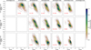 |
Fig. C.2 [Mg/Fe] versus [Fe/H] distribution of the stars in common between APOGEE-2 and GALAH in the same spatial bins as for Fig. C.1. |
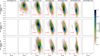 |
Fig. C.3 Same as Fig. C.2 but here the 2d histogram show the relative distribution using the ‘original’ GALAH data instead of the translated ones. |
Appendix D [Fe/H] and [Mg/Fe] distribution without the transformation of the SPECTROTRANSLATOR
In Fig. D.1, we show the [Fe/H] and [Mg/Fe] distribution across the Galaxy by combining the APOGEE-2 and GALAH samples, but using the ‘original’ values for the latter, instead of the transformed values as in the Sect. 4.3. Contrary to what shown in Sect. 4.3, one can see that without the transformation made by the SPECTROTRANSLATOR algorithm, the median [Fe/H] and [Mg/Fe] are very different when the APOGEE-2 and GALAH data are combined than when the only APOGEE-2 data are used. In particular, we can see that close to the Galactic midplane in the inner Galaxy, the median [Fe/H] and [Mg/Fe] values present a significant change, with a more conic profile when the GALAH data are used. Furthermore, we can see that the regions without APOGEE-2 data stand apart to the other area. This is particularly visible in R= –5 kpc Z= 2 kpc in both [Fe/H] and [Mg/Fe]. Comparing this figure with Fig. 17 shows the strength of the SPECTROTRANSLATOR algorithm, since when the algorithm is used we preserved the global structure of the Galaxy measured with the APOGEE-2 data only, contrary to when the “original” GALAH data are used. Nevertheless, it is interesting to note here that the vertical asymmetry in the median metallicity reported in Sect. 4.3 is still visible even when using the “original” GALAH data, since most of the stars in the outer disc originate from the APOGEE-2 sample.
References
- Abadi, M., Agarwal, A., Barham, P., et al. 2016, arXiv e-prints [arXiv: 1603.04467] [Google Scholar]
- Abdurro’uf, Accetta, K., Aerts, C., et al. 2022, ApJS, 259, 35 [NASA ADS] [CrossRef] [Google Scholar]
- Allende Prieto, C. 2016, Astron. Nachr., 337, 837 [NASA ADS] [CrossRef] [Google Scholar]
- Antoja, T., Helmi, A., Romero-Gómez, M., et al. 2018, Nature, 561, 360 [Google Scholar]
- Astropy Collaboration (Price-Whelan, A. M., et al.) 2018, AJ, 156, 123 [Google Scholar]
- Bastian, N., & Lardo, C. 2018, ARA&A, 56, 83 [Google Scholar]
- Bensby, T., Feltzing, S., Gould, A., et al. 2017, A&A, 605, A89 [NASA ADS] [CrossRef] [EDP Sciences] [Google Scholar]
- Bialek, S., Fabbro, S., Venn, K. A., et al. 2020, MNRAS, 498, 3817 [CrossRef] [Google Scholar]
- Binney, J., & Vasiliev, E. 2023, MNRAS, 520, 1832 [NASA ADS] [CrossRef] [Google Scholar]
- Binney, J., & Vasiliev, E. 2024, MNRAS, 527, 1915 [Google Scholar]
- Bowen, I. S., & Vaughan, Jr., A. H. 1973, Appl. Opt., 12, 1430 [NASA ADS] [CrossRef] [Google Scholar]
- Buder, S., Sharma, S., Kos, J., et al. 2021, MNRAS, 506, 150 [NASA ADS] [CrossRef] [Google Scholar]
- Casey, A. R., Hogg, D. W., Ness, M., et al. 2016, arXiv e-prints [arXiv: 1603.03040] [Google Scholar]
- Chollet, F. 2015, Keras, https://github.com/keras-team/keras [Google Scholar]
- Clarke, J. P., Wegg, C., Gerhard, O., et al. 2019, MNRAS, 489, 3519 [Google Scholar]
- Conroy, C., Naidu, R. P., Garavito-Camargo, N., et al. 2021, Nature, 592, 534 [NASA ADS] [CrossRef] [Google Scholar]
- Cooper, A. P., Koposov, S. E., Prieto, C. A., et al. 2023, ApJ, 947, 37 [NASA ADS] [CrossRef] [Google Scholar]
- Dalton, G., Trager, S. C., Abrams, D. C., et al. 2012, SPIE, 8446, 84460P [NASA ADS] [Google Scholar]
- de Jong, J. T. A., Yanny, B., Rix, H.-W., et al. 2010, ApJ, 714, 663 [NASA ADS] [CrossRef] [Google Scholar]
- de Jong, R. S., Agertz, O., Berbel, A. A., et al. 2019, The Messenger, 175, 3 [NASA ADS] [Google Scholar]
- Eilers, A.-C., Hogg, D. W., Rix, H.-W., et al. 2022, ApJ, 928, 23 [NASA ADS] [CrossRef] [Google Scholar]
- Fabbro, S., Venn, K. A., O’Briain, T., et al. 2018, MNRAS, 475, 2978 [Google Scholar]
- Flaugher, B., & Bebek, C. 2014, SPIE, 9147, 91470S [NASA ADS] [Google Scholar]
- Fukushima, K. 1975, Biol. Cybernet., 20, 121 [CrossRef] [Google Scholar]
- Gaia Collaboration (Recio-Blanco, A., et al.) 2023, A&A, 674, A38 [CrossRef] [EDP Sciences] [Google Scholar]
- García Pérez, A. E., Allende Prieto, C., Holtzman, J. A., et al. 2016, AJ, 151, 144 [Google Scholar]
- Gilmore, G., Randich, S., Worley, C. C., et al. 2022, A&A, 666, A120 [NASA ADS] [CrossRef] [EDP Sciences] [Google Scholar]
- Glorot, X., Bordes, A., & Bengio, Y. 2011, in Proceedings of Machine Learning Research, 15, Proceedings of the Fourteenth International Conference on Artificial Intelligence and Statistics, eds. G. Gordon, D. Dunson, & M. Dudík (Fort Lauderdale, FL, USA: PMLR), 315 [Google Scholar]
- Gómez, F. A., White, S. D. M., Marinacci, F., et al. 2016, MNRAS, 456, 2779 [Google Scholar]
- Gratton, R., Bragaglia, A., Carretta, E., et al. 2019, A&ARv, 27, 8 [Google Scholar]
- Guiglion, G., Nepal, S., Chiappini, C., et al. 2024, A&A, 682, A9 [NASA ADS] [CrossRef] [EDP Sciences] [Google Scholar]
- Gunn, J. E., Siegmund, W. A., Mannery, E. J., et al. 2006, AJ, 131, 2332 [NASA ADS] [CrossRef] [Google Scholar]
- Harris, W. E. 1996, AJ, 112, 1487 [Google Scholar]
- Harris, W. E. 2010, arXiv e-prints [arXiv:1012.3224] [Google Scholar]
- Hayden, M. R., Bovy, J., Holtzman, J. A., et al. 2015, ApJ, 808, 132 [Google Scholar]
- Haywood, M., Di Matteo, P., Lehnert, M. D., et al. 2018, ApJ, 863, 113 [Google Scholar]
- Haywood, M., Snaith, O., Lehnert, M. D., Di Matteo, P., & Khoperskov, S. 2019, A&A, 625, A105 [NASA ADS] [CrossRef] [EDP Sciences] [Google Scholar]
- He, K., Zhang, X., Ren, S., & Sun, J. 2016, in 2016 IEEE Conference on Computer Vision and Pattern Recognition (CVPR), 1 [Google Scholar]
- Hegedus, V., Mészáros, S., Jofré, P., et al. 2023, A&A, 670, A107 [NASA ADS] [CrossRef] [EDP Sciences] [Google Scholar]
- Hinton, G. E., Srivastava, N., Krizhevsky, A., Sutskever, I., & Salakhutdinov, R. R. 2012, arXiv e-prints [arXiv:1207.0580] [Google Scholar]
- Ho, A. Y. Q., Rix, H.-W., Ness, M. K., et al. 2017, ApJ, 841, 40 [CrossRef] [Google Scholar]
- Hochreiter, S., Bengio, Y., Frasconi, P., & Schmidhuber, J. 2001, in A Field Guide to Dynamical Recurrent Neural Networks, eds. S. C. Kremer, & J. F. Kolen (IEEE Press) [Google Scholar]
- Ibata, R. A., & Razoumov, A. O. 1998, A&A, 336, 130 [NASA ADS] [Google Scholar]
- Ibata, R., Diakogiannis, F. I., Famaey, B., & Monari, G. 2021, ApJ, 915, 5 [NASA ADS] [CrossRef] [Google Scholar]
- Imig, J., Price, C., Holtzman, J. A., et al. 2023, ApJ, 954, 124 [CrossRef] [Google Scholar]
- Jin, S., Trager, S. C., Dalton, G. B., et al. 2024, MNRAS, 530, 2688 [NASA ADS] [CrossRef] [Google Scholar]
- Jofré, P., Heiter, U., & Soubiran, C. 2019, ARA&A, 57, 571 [Google Scholar]
- Johnson, J. W., Weinberg, D. H., Vincenzo, F., et al. 2021, MNRAS, 508, 4484 [NASA ADS] [CrossRef] [Google Scholar]
- Jönsson, H., Allende Prieto, C., Holtzman, J. A., et al. 2018, AJ, 156, 126 [Google Scholar]
- Katz, D., Gómez, A., Haywood, M., Snaith, O., & Di Matteo, P. 2021, A&A, 655, A111 [NASA ADS] [CrossRef] [EDP Sciences] [Google Scholar]
- Kazantzidis, S., Bullock, J. S., Zentner, A. R., Kravtsov, A. V., & Moustakas, L. A. 2008, ApJ, 688, 254 [Google Scholar]
- Kingma, D. P., & Ba, J. 2014, arXiv e-prints [arXiv: 1412.6980] [Google Scholar]
- Kollmeier, J. A., Zasowski, G., Rix, H.-W., et al. 2017, ArXiv e-prints, [arXiv:1711.03234] [Google Scholar]
- Kordopatis, G., Binney, J., Gilmore, G., et al. 2015a, MNRAS, 447, 3526 [Google Scholar]
- Kordopatis, G., Wyse, R. F. G., Gilmore, G., et al. 2015b, A&A, 582, A122 [NASA ADS] [CrossRef] [EDP Sciences] [Google Scholar]
- Kordopatis, G., Recio-Blanco, A., Schultheis, M., & Hill, V. 2020, A&A, 643, A69 [NASA ADS] [CrossRef] [EDP Sciences] [Google Scholar]
- Kos, J., Lin, J., Zwitter, T., et al. 2017, MNRAS, 464, 1259 [NASA ADS] [CrossRef] [Google Scholar]
- Laporte, C. F. P., Gómez, F. A., Besla, G., Johnston, K. V., & Garavito-Camargo, N. 2018a, MNRAS, 473, 1218 [NASA ADS] [CrossRef] [Google Scholar]
- Laporte, C. F. P., Johnston, K. V., Gómez, F. A., Garavito-Camargo, N., & Besla, G. 2018b, MNRAS, 481, 286 [Google Scholar]
- Laporte, C. F. P., Belokurov, V., Koposov, S. E., Smith, M. C., & Hill, V. 2020a, MNRAS, 492, L61 [Google Scholar]
- Laporte, C. F. P., Famaey, B., Monari, G., et al. 2020b, A&A, 643, L3 [EDP Sciences] [Google Scholar]
- Li, Z., Gerhard, O., Shen, J., Portail, M., & Wegg, C. 2016, ApJ, 824, 13 [NASA ADS] [CrossRef] [Google Scholar]
- Lian, J., Zasowski, G., Hasselquist, S., et al. 2020, MNRAS, 497, 3557 [NASA ADS] [CrossRef] [Google Scholar]
- Lian, J., Zasowski, G., Hasselquist, S., et al. 2021, MNRAS, 500, 282 [Google Scholar]
- Lundberg, S., & Lee, S.-I. 2017, arXiv e-prints [arXiv:1705.07874] [Google Scholar]
- Majewski, S. R., Schiavon, R. P., Frinchaboy, P. M., et al. 2017, AJ, 154, 94 [NASA ADS] [CrossRef] [Google Scholar]
- Marigo, P., Girardi, L., Bressan, A., et al. 2008, A&A, 482, 883 [NASA ADS] [CrossRef] [EDP Sciences] [Google Scholar]
- Martig, M., Minchev, I., Ness, M., Fouesneau, M., & Rix, H.-W. 2016, ApJ, 831, 139 [CrossRef] [Google Scholar]
- Masseron, T., Garcia-Hernández, D. A., Mészáros, Sz., et al. 2019, A&A, 622, A191 [NASA ADS] [CrossRef] [EDP Sciences] [Google Scholar]
- Mészáros, S., Masseron, T., García-Hernández, D. A., et al. 2020, MNRAS, 492, 1641 [Google Scholar]
- Mészáros, S., Masseron, T., Fernández-Trincado, J. G., et al. 2021, MNRAS, 505, 1645 [Google Scholar]
- Minchev, I., Famaey, B., Quillen, A. C., et al. 2012a, A&A, 548, A127 [NASA ADS] [CrossRef] [EDP Sciences] [Google Scholar]
- Minchev, I., Famaey, B., Quillen, A. C., et al. 2012b, A&A, 548, A126 [NASA ADS] [CrossRef] [EDP Sciences] [Google Scholar]
- Minchev, I., Chiappini, C., & Martig, M. 2013, A&A, 558, A9 [CrossRef] [EDP Sciences] [Google Scholar]
- Minchev, I., Chiappini, C., & Martig, M. 2014, MNRAS, 298, 130 [Google Scholar]
- Minchev, I., Martig, M., Streich, D., et al. 2015, ApJ, 804, L9 [NASA ADS] [CrossRef] [Google Scholar]
- Minchev, I., Steinmetz, M., Chiappini, C., et al. 2017, ApJ, 834, 27 [Google Scholar]
- Nandakumar, G., Hayden, M. R., Sharma, S., et al. 2022, MNRAS, 513, 232 [CrossRef] [Google Scholar]
- Ness, M., Hogg, D. W., Rix, H. W., Ho, Anna. Y. Q., & Zasowski, G. 2015, ApJ, 808, 16 [NASA ADS] [CrossRef] [Google Scholar]
- Pancino, E., Romano, D., Tang, B., et al. 2017, A&A, 601, A112 [NASA ADS] [CrossRef] [EDP Sciences] [Google Scholar]
- Pedregosa, F., Varoquaux, G., Gramfort, A., et al. 2011, JMLR, 12, 2825 [Google Scholar]
- Põder, S., Benito, M., Pata, J., et al. 2023, A&A, 676, A134 [NASA ADS] [CrossRef] [EDP Sciences] [Google Scholar]
- Portail, M., Gerhard, O., Wegg, C., & Ness, M. 2017, MNRAS, 465, 1621 [NASA ADS] [CrossRef] [Google Scholar]
- Price-Whelan, A. M., Hogg, D. W., Rix, H.-W., et al. 2020, ApJ, 895, 2 [NASA ADS] [CrossRef] [Google Scholar]
- Purcell, C. W., Bullock, J. S., & Kazantzidis, S. 2010, MNRAS, 404, 1711 [NASA ADS] [Google Scholar]
- Queiroz, A. B. A., Anders, F., Chiappini, C., et al. 2020, A&A, 638, A76 [NASA ADS] [CrossRef] [EDP Sciences] [Google Scholar]
- Queiroz, A. B. A., Anders, F., Chiappini, C., et al. 2023, A&A, 673, A155 [NASA ADS] [CrossRef] [EDP Sciences] [Google Scholar]
- Randich, S., Gilmore, G., Magrini, L., et al. 2022, A&A, 666, A121 [NASA ADS] [CrossRef] [EDP Sciences] [Google Scholar]
- Recio-Blanco, A., de Laverny, P., Palicio, P. A., et al. 2023, A&A, 674, A29 [NASA ADS] [CrossRef] [EDP Sciences] [Google Scholar]
- Ribeiro, M. T., Singh, S., & Guestrin, C. 2018, in Proceedings of the Thirty-Second AAAI Conference on Artificial Intelligence and Thirtieth Innovative Applications of Artificial Intelligence Conference and Eighth AAAI Symposium on Educational Advances in Artificial Intelligence, AAAI’18/IAAI’18/EAAI’18 (New Orleans, Louisiana, USA: AAAI Press), 1527 [Google Scholar]
- Rojas-Arriagada, A., Zoccali, M., Schultheis, M., et al. 2019, A&A, 626, A16 [NASA ADS] [CrossRef] [EDP Sciences] [Google Scholar]
- Ruiz-Lara, T., Gallart, C., Bernard, E. J., & Cassisi, S. 2020, Nat. Astron., 4, 965 [NASA ADS] [CrossRef] [Google Scholar]
- Salimans, T., & Kingma, D. P. 2016, arXiv e-prints [arXiv: 1602.07868] [Google Scholar]
- Samek, W., Wiegand, T., & Müller, K.-R. 2017, arXiv e-prints [arXiv: 1708.08296] [Google Scholar]
- Sanders, J. L., Smith, L., & Evans, N. W. 2019, MNRAS, 488, 4552 [NASA ADS] [CrossRef] [Google Scholar]
- Schiavon, R. P., Phillips, S. G., Myers, N., et al. 2024, MNRAS, 528, 1393 [CrossRef] [Google Scholar]
- Schlafly, E. F., & Finkbeiner, D. P. 2011, ApJ, 737, 103 [Google Scholar]
- Schlegel, D. J., Finkbeiner, D. P., & Davis, M. 1998, ApJ, 500, 525 [Google Scholar]
- Sellwood, J. A., & Binney, J. J. 2002, MNRAS, 336, 785 [Google Scholar]
- Sestito, F., Longeard, N., Martin, N. F., et al. 2019, MNRAS, 46 [Google Scholar]
- Shapley, L. S. 1953, 17. A Value for n-Person Games, eds. H. W. Kuhn, & A. W. Tucker (Princeton: Princeton University Press), 307 [Google Scholar]
- Sheinis, A., Anguiano, B., Asplund, M., et al. 2015, JATIS, 1, 035002 [NASA ADS] [Google Scholar]
- Slack, D., Hilgard, S., Jia, E., Singh, S., & Lakkaraju, H. 2019, arXiv e-prints [arXiv: 1911.02508] [Google Scholar]
- Sormani, M. C., Binney, J., & Magorrian, J. 2015, MNRAS, 449, 2421 [NASA ADS] [CrossRef] [Google Scholar]
- Srivastava, N., Hinton, G., Krizhevsky, A., Sutskever, I., & Salakhutdinov, R. 2014, JMLR, 15, 1929 [Google Scholar]
- Steinmetz, M., Zwitter, T., Siebert, A., et al. 2006, AJ, 132, 1645 [Google Scholar]
- Thomas, G. F., & Battaglia, G. 2022, A&A, 660, A29 [NASA ADS] [CrossRef] [EDP Sciences] [Google Scholar]
- Thomas, G. F., Annau, N., McConnachie, A., et al. 2019, ApJ, 886, 10 [NASA ADS] [CrossRef] [Google Scholar]
- Ting, Y.-S., Conroy, C., Rix, H.-W., & Cargile, P. 2019, ApJ, 879, 69 [Google Scholar]
- Traven, G., Feltzing, S., Merle, T., et al. 2020, A&A, 638, A145 [NASA ADS] [CrossRef] [EDP Sciences] [Google Scholar]
- Tsantaki, M., Pancino, E., Marrese, P., et al. 2022, A&A, 659, A95 [NASA ADS] [CrossRef] [EDP Sciences] [Google Scholar]
- Tulio Ribeiro, M., Singh, S., & Guestrin, C. 2016, arXiv e-prints [arXiv: 1602.04938] [Google Scholar]
- Vasiliev, E., Belokurov, V., & Erkal, D. 2021, MNRAS, 501, 2279 [NASA ADS] [CrossRef] [Google Scholar]
- Velazquez, H., & White, S. D. M. 1999, MNRAS, 304, 254 [NASA ADS] [CrossRef] [Google Scholar]
- Villalobos, Á., & Helmi, A. 2008, MNRAS, 391, 1806 [Google Scholar]
- Wegg, C., Gerhard, O., & Portail, M. 2015, MNRAS, 450, 4050 [NASA ADS] [CrossRef] [Google Scholar]
- Wheeler, A., Ness, M., Buder, S., et al. 2020, ApJ, 898, 58 [Google Scholar]
- Wilson, J. C., Hearty, F. R., Skrutskie, M. F., et al. 2019, PASP, 131, 055001 [NASA ADS] [CrossRef] [Google Scholar]
- Wojtas, M., & Chen, K. 2020, arXiv e-prints [arXiv:2010.08973] [Google Scholar]
- Xiang, M., Ting, Y.-S., Rix, H.-W., et al. 2019, ApJS, 245, 34 [Google Scholar]
- Yan, H., Li, H., Wang, S., et al. 2022, The Innovation, 3, 100224 [NASA ADS] [CrossRef] [Google Scholar]
- Yanny, B., Newberg, H. J., Johnson, J. A., et al. 2009, ApJ, 700, 1282 [NASA ADS] [CrossRef] [Google Scholar]
- Zasowski, G., Schultheis, M., Hasselquist, S., et al. 2019, ApJ, 870, 138 [NASA ADS] [CrossRef] [Google Scholar]
- Zhao, G., Zhao, Y.-H., Chu, Y.-Q., Jing, Y.-P., & Deng, L.-C. 2012, RAA, 12, 723 [Google Scholar]
Hereafter, we refer to these quantities with ‘spectral parameters’.
This assumes that the velocities measured by surveys A and B are relatively similar to each other, which is expected to be the case for our case for all stars except those with a very low S/N and for some binary systems.
We decided to define the depth of the network (n) such that it corresponds to the number of blocks needed to reach the central layer, as the network is constructed symmetrically around it.
A linear layer performs a linear transformation of the inputs (x) such that y = Wx + b, where W represents the weights and b the bias, which are learned by the algorithm. Therefore, they are equal to a fully connected dense layer without any activation function.
The STAR_BAD flag is set for a star if any of TEFF_BAD,LOGG_BAD, CHI2_BAD, COLORTE_BAD, ROTATION_BAD,SN_BAD or GRIDEDGE_BAD OCCUR is set.
The loss function is the metric that quantify the disparity between the transformed and the actual output values.
Note that both methods are already implemented in the public version of the SPECTROTRANSLATOR.
For the translated GALAH sample, the uncertainties of a parameter X are computed as dX =(X_PRED_84-X_PRED_16)/2.
The figure was made using the kernel density estimator included in the python package SCKIT-LEARN (Pedregosa et al. 2011).
All Tables
Mean [Fe/H] and [Mg/Fe] derived for the 4 globular clusters studied here using the APOGEE-2, the ‘original’ GALAH, and the translated GALAH into APOGEE-2 data.
Metadata for all sources from the GALAH DR3 catalogue transformed onto the APOGEE-2 DR17 base.
All Figures
|
Fig. 1 Sketch of the main part of the SPECTROTRANSLATOR algorithm. The difference between the spectroscopic parameters of catalogue A and B (∆Xa→b) are computed in a deep fully connected network, where the inputs are composed of the spectroscopic parameters from catalogue A, and of photometric colours. The deep network of depth-n is made by a series of n blocks of progressively increasing complexity, until a central layer of maximum complexity, before decreasing symmetrically. Each block is composed of a REsNET-like unit (see Sect. 2.1), illustrated on the right part, and of a linear layer that adjust the number of feature (nf ) between each depth. Finally, the difference predicted by the deep network are added to the spectroscopic parameters of catalogue A to compute the parameters values expressed in the base of catalogue B. |
| In the text | |
|
Fig. 2 Sky coverage (in Galactic coordinates) of the 16583 stars in common (in blue) between APOGEE-2 DR17 and GALAH DR3 that fullfil the criteria listed in Sect. 3.1, overlaid on the spatial coverage of these two surveys (in grey and orange, respectively). |
| In the text | |
|
Fig. 3 Variation of the metallicity (upper panel) between the APOGEE and GALAH values as function of the effective temperature and colour-coded by the median surface gravity from GALAH, for the stars of the training/validation sample (see Sect. 3.1). The lower panel shows the variation of the surface gravity between the two surveys as function of the effective temperature and median metallicity values from GALAH for the same stars. |
| In the text | |
|
Fig. 4 Evolution of the loss function as a function of the epoch for the intrinsic network (on the top panel), and of the extrinsic network (on the bottom panel). The loss of the training sample is shown by the blue curve, while the one of the validation sample is shown by the orange line. |
| In the text | |
|
Fig. 5 Comparison between the coverage of the parameter space for stars in the training sample using the original GALAH data (in purple, left panels), the original APOGEE-2 data (in blue, middle panels) and the parameters transformed from the GALAH into the APOGEE-2 base by the SPECTROTRANSLATOR algorithm (in orange, right panels). The contours in the right and middle panels depict the 1, 10, and 100 stars per bin limits in the selected GALAH DR3 catalogue (refer to Section 3.1.1) and APoGEE DR17 (refer to Section 3.1.2), respectively. |
| In the text | |
|
Fig. 6 Variation of the residuals between “original” GALAH (XA) and APOGEE-2 (XB) values for each output parameters. Left: validation set shown with black points, while the shaded areas correspond to the 1, 2, and 3σ around the local mean of the residual obtained from the training set. Bins where the number of stars in the training set is lower than five are not shown, due to the poor statistic in them. The horizontal dashed lines correspond to the average 3σ of the residuals. Right panels: the coloured histograms show the difference between the ‘original’ GALAH (XA) and APOGEE-2 (XB), and black curve shows the Gaussian fitted to this histogram used to measure the average mean and standard deviation of the residuals, which are quoted on the right panels of each parameters. |
| In the text | |
|
Fig. 7 Similar to Fig. 6, but with residuals between the transformed |
| In the text | |
|
Fig. 8 Relative importance that each feature has on the transformation of the parameters in the APOGEE-2 base, computed from the mean absolute SHAP values (see Sect. 3.3.2). |
| In the text | |
|
Fig. 9 Relation between the residuals of the transformed and the ‘original’ APOGEE-2 values for effective temperature as a function of the S/N of the input data is depicted for two cases: when colours are used for the transformation (circles) and when colours are not used (squares). The red line shows the percentage increase in the residual of the effective temperature for the transformation without colours compared to the transformation using colours. |
| In the text | |
|
Fig. 10 Comparison between the difference of the l.o.s. velocity measured by GALAH and APOGEE-2 on the top panel, as well as the difference of the velocity transformed by the SPECTROTRANSLATOR algorithm and the APOGEE-2 data on the bottom panel, as a function of the l.o.s velocity measured by APOGEE-2. In both cases, the symbols show the stars of the training set. The histograms on the right panels show the distribution of the difference between the l.o.s. velocity measured by GALAH and APOGEE-2 (on top) and between the transformed GALAH l.o.s and the “original” APOGEE-2 values. |
| In the text | |
|
Fig. 11 Relative importance of each feature in the transformation of the l.o.s. velocity from the GALAH to the APOGEE-2 base. |
| In the text | |
|
Fig. 12 [Fe/H] as function of the effective temperature (top row) and surface gravity (lower row) for 4 globular clusters. The parameters from the “original” GALAH data are shown by the orange points, while the value transformed on the APOGEE-2 base by the SPECTROTRANSLATOR are shown by the blue circles. The red points show the values for the stars present in the APOGEE-2 DR17 dataset. The filled circles highlight the stars observed by both APOGEE-2 and GALAH, while the open circles show the stars that have been observed either by APOGEE-2 or GALAH. The colourised triangles with the error bars indicate the average uncertainties on the individual [Fe/H] measurements in the corresponding catalogue. The horizontal red and blue lines indicates the mean metallicity of the cluster measured using the ‘original’ APOGEE-2 and transformed GALAH values, respectively. |
| In the text | |
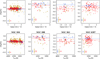 |
Fig. 13 Same as Fig. 12 but for [Mg/Fe] instead of metallicity. |
| In the text | |
|
Fig. 14 [Mg/Fe] values measured by APOGEE-2 and GALAH for the six stars of NGC 362 observed by both surveys (in black triangle). The points show the distribution of stars from the training/validation sample in the same range of temperature, surface gravity and metallicity than the stars of NGC 362. They are colour coded by the difference between the [Mg/Fe] transformed by the SPECTROTRANSLATOR and the ‘original’ APOGEE-2. The dashed line shows the 1:1 relation in the [Mg/Fe] measurement between APOGEE-2 and GALAH. |
| In the text | |
|
Fig. 15 Kiel diagram for different ranges of Galactocentric radii and vertical elevations from the midplane. The 2D histogram shows the relative distribution (made with a kernel density estimator) of the transformed GALAH data in each spatial bin. The grey iso-density contours are plotted at the 1, 5, 10, 30, 50, and 70% of the maximum density for the stars from APOGEE-2. In each bin, NG and NA refer to the number of stars from the GALAH and APOGEE catalogues, respectively. The horizontal dashed red lines show the upper and lower limit for the selection of giant stars used in Sect. 4. |
| In the text | |
|
Fig. 16 [Mg/Fe] versus [Fe/H] distribution of the selected giant stars 2.5 > log(ɡ) > 1.5 dex in the same spatial bins as for Fig. 15. |
| In the text | |
|
Fig. 17 Edge-on view of the global maps of the Milky Way, showing the number of stars observed (upper panels), the median [Fe/H] (middle panels) and median [Mg/Fe] (lower panels) distribution for the APOGEE-2 sample only (left), and combined to the transformed GALAH data (right side) in 0.2 kpc × 0.2 kpc bins. On the upper left panel, the grey area illustrates the region not covered at all by the APOGEE-2 survey, but that has been observed by the GALAH survey. In each panel, the dashed black line shows the Galactic mid-plane, and the yellow circle indicates the location of the Sun. We note that R preserve the sign of the X-axis to show the opposite side of the Galaxy. |
| In the text | |
|
Fig. 18 Radial gradients of the metallicity (left) and [Mg/Fe] (right) for different elevations from the Galactic midplane. The upper row shows the profile using only the APOGEE-2 data, the middle row combining them with the ‘original’ GALAH values, and the lower row combining the APOGEE-2 data with the translated GALAH data. The trends are computed as running medians in bins of 0.5 kpc, with a 50 percent overlap, provided that at least 20 stars are available to compute the median. The shaded areas represent the uncertainty on the median (obtained from the 16th and 84th percentile of 1000 bootstrap samples). The continuous lines show the trend above the Galactic midplane (Z > 0), and the dashed lines the trend below the midplane (Z < 0). |
| In the text | |
|
Fig. 19 Vertical gradients of the metallicity (left panel) and [Mg/Fe] (right panel) for different radial distance from the Galactic centre. The upper row shows the profile using only the APOGEE-2 data, the middle row combining them with the ‘original’ GALAH values, and the lower row combining the APOGEE-2 data with the translated GALAH data. The trends are computed as running medians in bins of 0.2 kpc, with a 50% overlap, provided that at least 20 stars are available to compute the median. The shaded areas represent the uncertainty on the median (obtained from the 16th and 84th percentile of 1000 bootstrap samples). |
| In the text | |
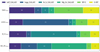 |
Fig. B.1 Same as Fig. 8 but for metal-poor stars ([Fe/H]< –1.0). |
| In the text | |
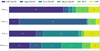 |
Fig. B.2 Same as Fig. 8 but for metal-rich stars ([Fe/H]> –0.4). |
| In the text | |
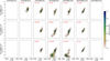 |
Fig. C.1 Same as Fig. 15 but for the stars in common between APOGEE-2 and GALAH. |
| In the text | |
|
Fig. C.2 [Mg/Fe] versus [Fe/H] distribution of the stars in common between APOGEE-2 and GALAH in the same spatial bins as for Fig. C.1. |
| In the text | |
|
Fig. C.3 Same as Fig. C.2 but here the 2d histogram show the relative distribution using the ‘original’ GALAH data instead of the translated ones. |
| In the text | |
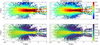 |
Fig. D.1 Same as Fig. 17 but with the ‘original’ [Fe/H] and [Mg/Fe] from GALAH. |
| In the text | |
Current usage metrics show cumulative count of Article Views (full-text article views including HTML views, PDF and ePub downloads, according to the available data) and Abstracts Views on Vision4Press platform.
Data correspond to usage on the plateform after 2015. The current usage metrics is available 48-96 hours after online publication and is updated daily on week days.
Initial download of the metrics may take a while.