| Issue |
A&A
Volume 690, October 2024
|
|
|---|---|---|
| Article Number | A46 | |
| Number of page(s) | 23 | |
| Section | Planets and planetary systems | |
| DOI | https://doi.org/10.1051/0004-6361/202449981 | |
| Published online | 27 September 2024 | |
Early Planet Formation in Embedded Disks (eDisk)
XVI. Asymmetric dust disk driving a multicomponent molecular outflow in the young Class 0 protostar GSS30 IRS3
1
European Southern Observatory,
3107, Alonso de Córdova,
Santiago de Chile
2
Academia Sinica Institute of Astronomy & Astrophysics,
11F of Astronomy-Mathematics Building, AS/NTU, No.1, Sec. 4, Roosevelt Rd,
Taipei
106216,
Taiwan,
ROC
3
National Radio Astronomy Observatory,
520 Edgemont Rd,
Charlottesville,
VA,
22903,
USA
4
Niels Bohr Institute, University of Copenhagen,
Jagtvej 155A,
2200
Copenhagen N.,
Denmark
5
Korea Astronomy and Space Science Institute,
776 Daedeok-daero, Yuseong-gu,
Daejeon
34055,
Republic of Korea
6
University of Virginia,
530 McCormick Rd.,
Charlottesville,
Virginia
22904,
USA
7
Department of Physics and Astronomy, Graduate School of Science and Engineering, Kagoshima University,
1-21-35 Korimoto, Kagoshima,
Kagoshima
890-0065,
Japan
8
Department of Earth Science Education, Seoul National University,
1 Gwanak-ro, Gwanak-gu,
Seoul
08826,
Republic of Korea
9
SNU Astronomy Research Center, Seoul National University,
1 Gwanak-ro, Gwanak-gu,
Seoul
08826,
Republic of Korea
10
Division of Astronomy and Space Science, University of Science and Technology,
217 Gajeong-ro, Yuseong-gu,
Daejeon
34113,
Republic of Korea
11
Department of Astronomy, University of Illinois,
1002 West Green St,
Urbana,
IL
61801,
USA
12
Department of Astronomy, University of Michigan,
1085 S. University Ave.,
Ann Arbor,
MI
48109-1107,
USA
13
Institute for Astronomy, University of Hawai‘i at Mānoa,
2680 Woodlawn Dr.,
Honolulu,
HI
96822,
USA
Received:
14
March
2024
Accepted:
29
July
2024
Abstract
We present the results of the observations made within the ALMA Large Program called Early Planet Formation in Embedded disks of the Class 0 protostar GSS30 IRS3. Our observations included the 1.3 mm continuum with a resolution of 0″.05 (7.8 au) and several molecular species, including 12CO, 13CO, C18O, H2CO, and c-C3H2. The dust continuum analysis unveiled a disk-shaped structure with a major axis of ~200 au. We observed an asymmetry in the minor axis of the continuum emission suggesting that the emission is optically thick and the disk is flared. On the other hand, we identified two prominent bumps along the major axis located at distances of 26 and 50 au from the central protostar. The origin of the bumps remains uncertain and might be an embedded substructure within the disk or the temperature distribution and not the surface density because the continuum emission is optically thick. The 12CO emission reveals a molecular outflow consisting of three distinct components: a collimated component, an intermediate-velocity component exhibiting an hourglass shape, and a wider angle low-velocity component. We associate these components with the coexistence of a jet and a disk wind. The C18O emission traces both a circumstellar disk in Keplerian rotation and the infall of the rotating envelope. We measured a stellar dynamical mass of 0.35 ±0.09 M⊙.
Key words: stars: low-mass / stars: protostars / stars: winds, outflows / submillimeter: ISM / submillimeter: stars
Corresponding author; This email address is being protected from spambots. You need JavaScript enabled to view it.
© The Authors 2024
 Open Access article, published by EDP Sciences, under the terms of the Creative Commons Attribution License (https://creativecommons.org/licenses/by/4.0), which permits unrestricted use, distribution, and reproduction in any medium, provided the original work is properly cited.
This article is published in open access under the Subscribe to Open model. This email address is being protected from spambots. You need JavaScript enabled to view it. to support open access publication.
1 Introduction
Circumstellar disks arise as a direct consequence of the angular momentum conservation of rotating material from an infalling envelope (Shu & Terebey 1984; Shu et al. 1987). In these disks, planets are expected to form at some point during the star formation process. In the past decade, the efforts to understand planet formation have mainly been focused on Class II disks that have dispersed their envelopes. The advent of the Atacama Large Millimeter/submillimeter Array (ALMA) provided the needed sensitivity and spatial resolution to resolve structures inside disks such as rings, gaps, and dust traps (van der Marel et al. 2013; ALMA Partnership 2015). These structures are ubiquitous in the star-forming regions studied in different ALMA programs (e.g., Andrews et al. 2016; Long et al. 2018; Cieza et al. 2021) and may reflect the presence of planets (Zhang et al. 2015; Flock et al. 2015; Andrews et al. 2018).
If these substructures are the consequence of the presence of planets, we need to investigate the origin of planets in earlier evolutionary stages. The lack of sufficient mass to form the observed population of exoplanets in Class II disks (Manara et al. 2018) and the fact that Class 0/I disks are likely more massive and abundant in solids (Tychoniec et al. 2020; Tobin et al. 2020; Sheehan & Eisner 2017) supports the scenario in which planets are formed at earlier stages.
Dedicated high angular resolution observations millime- ter/submillimeter wavelengths have revealed the presence of substructures in the dust disks that surround some young Class 0/I sources (Sheehan & Eisner 2017, 2018; Segura-Cox et al. 2020; Sheehan et al. 2020), but the question remains whether these are ubiquitous and when they arise. To address this question, the ALMA Large Program called Early Planet Formation in Embedded disks (Ohashi et al. 2023, eDisk) aims to systematically study the origin of substructures in Class 0/I disks with ALMA at 1.3 mm (Band 6) and a spatial resolution of 0704. The sample comprises 12 Class 0 and 7 Class I protostars in nearby (d < 200 pc) star-forming regions. The program aims to detect indication of disk substructures that may indicate the presence of planets or the presence of giant spirals as a byproduct of gravitational instabilities.
The source GSS30 IRS3 was observed as part of the eDisk Large Program. It is part of the L1688 molecular cloud, located at a distance of ~ 138.4 ± 2.6 pc (Ortiz-León et al. 2018) based on recent Gaia measurements. GSS30 IRS3 is a deeply embedded protostar (Jørgensen et al. 2009) that was not detected at optical wavelengths, preventing a direct measurement of its distance from Gaia. Therefore, we assume that the distance to the source is similar to that of its host cloud. GSS30 IRS3 is classified as a Class 0 protostar with a bolometric luminosity (mmLbol) of 1.7 L⊙, and the bolometric temperature is 50 K (Ohashi et al. 2023). GSS30 IRS 3 was first detected by Tamura et al. (1991) and later observed at 2.7 mm at higher angular resolution in a focused paper on the three sources at GSS30 (Zhang et al. 1997). A molecular outflow was reported with single-dish observations taken at the James Clerk Maxwell Telescope (White et al. 2015) and later with ALMA (Friesen et al. 2018) in CO (2–1) at a resolution of ~1.″5.
In this paper, we present observations of GSS30 IRS3 at a very high angular resolution (07056) in the continuum (at 1.3 mm) and (~0715) in line emission (CO isotopologs, H2CO, and c-C3H2) as part of the eDisk ALMA Large Program. The paper is structured as follows: We describe the observations in Sect. 2. Then, we present the continuum, spectral line maps, and dust mass estimation in Sect. 3. Section 4 presents the molecular outflow analysis and the estimation of the dynamical mass of the protostar. We discuss the origin of the continuum asymmetries, the twisted feature observed in the C18O velocity map, and the coexistence of a jet and a wide-angle outflow in Sect. 5. Finally, we summarize the main results in Sect. 6.
2 Observation and data reduction
GSS30 IRS3 was observed with the ALMA 12-m array in Band 6 as part of the eDisk ALMA Large Program (project code: 2019.1.00261.L: PI: N. Ohashi). A separate DDT program (2019.A.00034.S: PI: J. Tobin) complements the eDisk data with shorter baselines for the same molecular lines for some sources. Observations toward GSS30 IRS3 from the Large Program were executed four times in October 2021 in configuration C43-8, while two executions were completed for the DDT program in June 2022 with configuration C43-5. Detailed information about the baseline length, the number of antennas, the precipitable water vapor, and the calibrators is provided in Ohashi et al. (2023, Table 3).
The correlator was set up in dual-polarization mode using four basebands. The first baseband was divided into four spectral windows to detect C18O (2–1), 13CO (2–1), H2CO (32,1–22,0), and SO (65–54) with a spectral resolution of ~0.17 km s–1 and a bandwidth of 58.59 MHz. Basebands 2 and 3 were set up with a bandwidth of 1875 MHz to detect the continuum. A spectral resolution of ~1.3 km s–1 was selected for the detection of several molecular lines (CH3 OH, SiO, DCN, H2CO, and c-C3H2), and these lines were identified and masked when measuring the continuum. The fourth baseband has a bandwidth of 937.5 MHz (0.64 km s–1 spectral resolution) to detect the continuum and the12 CO (2–1) line. The time on source for data from the Large Program was 2.75 h, and for the DDT program, the time on source was 0.5 h.
The ALMA data were calibrated using the standard ALMA calibration pipeline. Then, we self-calibrated the data using the Common Astronomy Software Applications package (McMullin et al. 2007, CASA) version 6.2.1 and 6.4.1 for 2019.1.00261.L and 2019.A.00034.S programs, respectively. The pipeline version numbers should be supplied in addition to the CASA number. Before performing the self-calibration, we first imaged the six executions and aligned the emission peaks using fixvis and fixplanets. After the alignment, we rescaled the flux in the UV plane to the execution on the 27 October. Then we proceeded with the self-calibration, but using the rescaled nonaligned data, first with four phase-only cycles and two phase and amplitude cycles of the short-baseline data. Next, we performed joint self-calibration of the long- and short-baseline data and proceeded with four iterations of self-calibration in phase-only mode. Finally, the self-calibration solutions were applied to both the continuum and the spectral line data, and the task TCLEAN was used to produce continuum and spectral line images after continuum subtraction. The final image is a combination of the short and long configurations. We adopted a Briggs robust parameter equal to 0 for the continuum image and 0.5 for the spectral line data as a compromise between sensitivity and resolution. We also adopted a Briggs robust parameter equal to 2 for the H2CO and c-C3H2 spectral to enhance the sensitivity. The spectral line data were tapered at 2000 kλ to bring out larger- scale structures. Primary beam correction was applied before inferring physical parameters from the images. The angular resolution of the continuum maps is 07056 (7.8 au at a distance of 138 pc), with a maximum recoverable angular scale of 279, which is also the nominal value for Configuration 5 and a field of view of ~22″. The absolute flux calibration uncertainty in Band 6 is estimated to be 10%. A more detailed explanation of the reduction procedure can be found in Ohashi et al. (2023).
3 Results
3.1 Dust emission
Figure 1 shows the dust emission at 1.3 mm of GSS30 IRS3 at an angular resolution of 07068×07045 (position angle of 76.61°), obtained using a robust parameter equal to 0. The continuum emission traces a disk-like structure around the central protostar with a high inclination angle. The deconvolved disk size is 0755×0717 (76×23 au) estimated from a 2D Gaussian fitting (see Table 1). The best-fit peak intensity is 3.87 ± 0.04 mJy beam–1 at the Gaussian central position RA = 16h26m21.715s, Dec= –24°22’51.″709. The flux density obtained from the Gaussian fitting is 123.6 ± 1.2 mJy. The continuum emission measured above a 5σ contour has major and minor axes of 1743×0762 (~198 × ~86 au), while the peak intensity and the flux density obtained by this method are 6.38 mJy beam–1 and 133.7 mJy, respectively. Since the residuals from the Gaussian fitting show that the fit is far from perfect (see the model and residual in Fig. 1), and because a fitting attempt using 2D Gaussian components did not converge either, we adopted the values of the flux density and size inferred above the 5σ contour in the analysis section. Assuming a geometrically flat and axisymmetric disk, we can estimate the disk inclination as cos i = b/a, where a and b are the major and minor axes. The inclination derived using the deconvolved Gaussian fitting is 71.7 ± 0.3°, while using the 5σ contour, we obtained 64.3 ± 1.5° with the same position angle in both cases (109°). Because the quality of the Gaussian fitting is poor, we adopted a value of 64.3° as the most reliable inclination estimation. We note that when the disk is geometrically thick, this value should be treated as a lower limit. Additionally, the dust disk exhibits a boxy shape (see Sect. 5.1 for further discussions).
Moreover, we also detected the dust emission of another source (GSS30 IRS1) in the field of view (see Appendix C.1 for further information).
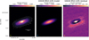 |
Fig. 1 ALMA continuum observations of GSS30 IRS at 1.3 mm. Left: continuum image of GSS30 IRS3. The white contours are 5, 10, 20, 40, 60, 80, 100, 130, 160, 190, and 220 times the rms (1σ = 18.5 µJy beam–1). Center: Model image of the Gaussian fit. Right: residual from the model image of the Gaussian fit. The white contours are –20, –10, 5, 10, 20, 40, 60, 80, 100, 130, 160, 190, and 220 times the rms. The dashed lines represent negative contours. The beam size is represented by the filled ellipse in the bottom left corner of the three images. |
Physical parameters of the continuum map using the task imfit rom CASA.
3.2 Brightness asymmetries
There are no apparent substructures in the disk surrounding GSS30 IRS3 (Fig. 1), such as clear spirals, gaps, or sharp rings, similar to those found in many more evolved Class II sources (Andrews et al. 2018). Instead, the image shows a striking asymmetry along the minor axis. To show this asymmetry more clearly, we performed a 1D cut along the minor axis centered on the peak derived from the Gaussian fitting (Fig. 2). Additionally, along the major axis lie two bumps on either side of the disk, located at 0″.18 (∼25 au) and 0″.36 (∼50 au) east and west from the disk center, respectively. There is only one bump along the minor axis, which could be due to a flared structure of the disk. The center of the bump is located at a deprojected distance of ∼20 au from the center of the disk. The radial brightness profile of the continuum emission is discussed in Sects. 5.1 and 5.2.
3.3 Mass of the dust disk
The mass of the dust disk surrounding GSS30 IRS3 was estimated under the assumption that the emission at 1.3 mm is optically thin and comes entirely from isothermal dust. We estimated the dust mass using the relation from Hildebrand (1983),
 (1)
(1)
where D is the distance to the source (138 pc), Bν(Td) is the Planck function at the observed frequency (225 GHz) at a dust temperature Td, and κν(2.3 cm2 g–1) is the absorption coefficient adopted from Beckwith et al. (1990). Sν is the flux density. We assumed two different values of the dust temperature to estimate the dust disk mass. The first temperature value we used was a fixed value of 20 K, which is commonly assumed for Class II sources (Pascucci et al. 2016). For the second temperature, we took into account the typical temperature of the disk based on the source luminosity. We derived this temperature using the formula T = 43(Lbol/Lsun)0.25 from Tobin et al. (2020), which was obtained from a grid of radiative transfer models. For our specific case of GSS30 IRS3, this formula provides a temperature of 49 K. Using these two temperature values, we calculated the mass of the dust disk using the flux density derived from the Gaussian fitting and the density calculated above the 5σ contour level. For the Gaussian fitting, we obtained a mass of the dust disk of 69.5 ± 2.6 M⊕ and 23.87 ± 0.90 M⊕ for a temperature of 20 K and 49 K, respectively. The dust mass estimation when using the flux density above the 5σ contour level provides values of 75.1 ± 2.9 M⊕ and 25.80 ± 0.99 M⊕ considering a temperature of 20 K and 49 K, respectively. The values that we derived are between 4.9 and 1.5 times more massive than those that were derived by Friesen et al. (2018), but their κν value is much higher (7.4 cm2 g–1) than the value used in this paper, so that we associate the differences with the adopted absorption coefficient. Compared to other Class 0 sources in the eDISK sample, we find relatively similar values to R CrA IRS 5N (protostellar mass of 0.3 M⊙) with a mass of the dust disk between 23.3 and 66.6 M⊕ (van’t Hoff et al. 2023) or L1527 (protostellar mass of 0.5 M⊙) with a mass of the dust disk between 38.9 and 97.4 M⊕ (Sharma et al. 2023). Finally, we note that the derived dust mass might be a lower limit to the actual mass because the inclined disk might be optically thick.
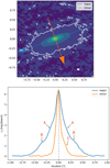 |
Fig. 2 Radial intensity profiles on the dust continuum emission. Top: 1.3 mm continuum image. The major (blue) and minor (orange) axes are overlaid and show the direction of the cuts. The white contours show the 3σ level. The coordinates of the central position are RA=16h26m21.715s, Dec= –24°22’51″.709, which is the peak position derived from the 2D Gaussian fitting. Bottom: radial intensity profile cuts along the major and minor axes of the continuum disk. The black arrows point to the bumps labeled A and B for the major axis, and C for the minor axis. The dashed line shows the position of the continuum peak of the major axis derived from the 2D Gaussian fitting. The arrows in the top panel point to the positive part of the axis. |
3.4 Gas emission
We report the detection of several molecular species and transitions: 12CO (2–1),13 CO (2–1), C18O (2–1), c-C3H2 (blended lines 60,6-51,5 and 61,6-50,5), c-C3H (51,4-42,3), c-C3H2 (52,4- 41,3), H2CO (30,3-20,2), and H2CO (32,2–22,1). The DCN (3-2), H2CO 32,1 – 22,0, SO (65–54), and SiO (5-4) lines are not detected. The systemic velocity is 2.84 km s–1 (which was derived from the C18O (2–1) diagram fitting discussed in Sect. 4.1). The moment maps of the detected molecular transitions are presented in Figs. 3–5, where we show integrated intensity (moment 0), mean velocity (moment 1), and peak intensity (moment 8) maps. A summary of the main properties of the detected lines including the angular resolution for each molecule is shown in Table 2, and an extensive description is provided in the following subsections.
3.4.1 12CO
The 12CO (2–1) emission line primarily traces a bipolar molecular outflow centered at the position of GSS30 IRS3 and perpendicular to the dust disk, as was also previously reported by Friesen et al. (2018) using a lower angular resolution and less sensitive observations. Our ALMA data reveal three different outflow components in morphology and velocity: a collimated inner high-velocity component, an intermediate velocity component with an hourglass or conical shape, and a wider-angle lower-velocity component that is more prominent in the northern lobe, which has a parabolic shape (see Fig. 6). The velocity channel maps of the 12CO (2–1) emission are presented in Fig. A.1 and the intensity-weighted velocity map in Fig. 3. In Fig. B.1 we plot the 12CO contours overlaid on a recent JWST image of the ρ Ophiuchus region (PI: Klaus Pontoppidan) where the H2 (0-0 S9) emission traces the outflow and very clearly delimits the cavity wall beyond the molecular outflow.
The collimated high-velocity component shows blueshifted emission to the northeast from the central source (spanning velocities between –19.9 and –18.7 km s–1 in the local standard of rest velocity) and redshifted emission to the southwest (23.2 to 23.8 km s–1; top left panel of Fig. 6). The JWST image reveals knots located at 4″.9 and 6″.7 from the center of the GSS3 0 IRS3 disk in the same direction as the blueshifted high-velocity component (right panel in Fig. B.1). Correcting the outflow velocities for the inclination of the system and considering that the inclination angle is a lower limit of the actual angle, the maximum deprojected velocity in the inner collimated high-velocity component is 52 km s–1. It is important to note that the deprojected velocity we derived is also a lower limit because the inclination angle is a lower limit of the actual angle. This deprojected velocity falls within the expected velocity range observed in jets associated with Class 0 sources (100 ± 50 km s–1, Lee et al. 2015; Jhan & Lee 2016; Podio et al. 2016; Yoshida et al. 2021).
The intermediate-velocity component of the outflow delineates an hourglass shape and spans velocities between –18.0 and –2.2 km s–1 for the blueshifted lobe and between 8.6 and 22.6 km s–1 for the redshifted lobe. Both redshifted and blueshifted emission are present at either side, as expected in outflows with a non-narrow opening angle and close to the plane of the sky (see the top right panel in Fig. 6). The wider-angle low- velocity component of the molecular outflow shows blueshifted emission between -1.6 and 1.6 km s–1m and redshifted emission between 5.4 and 7.9 km s–1. It is formed by an extended but well- defined northeast arc that is mostly seen at blueshifted velocities and by a less extended southwestern lobe where both blueshifted and redshifted components overlap in the same area of the sky (see the bottom left panel in Fig. 6).
We also report the detection of 12CO (2–1) in two other sources (GSS30 IRS1 and IRS2) that are in the ALMA field of view. The GSS30 IRS1 observations will be presented in a future paper, and the IRS2 detection is presented in Appendix C.2.
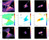 |
Fig. 3 Moment maps of the detected CO isotopologs. The left column shows 12CO (2–1) , the middle column shows 13CO (2–1) , and the right column shows C18O (2–1). The top row shows the peak intensity map, the center row shows the intensity-weighted velocity map, and the bottom row shows the integrated intensity map. The synthesized beam is represented as a filled ellipse at the bottom left side of every panel. The green contours represent the disk continuum emission with 10, 150, and 200 times the rms. The white contours represent 3, 5, 7, 9, 11, 13, and 15 times the rms (1σ = 9.5 mJy beam-1 km s–1) for the 12CO (2–1) moment 0 map; 5, 7, 9, 11, 13, and 15 times the rms (1σ = 2.7 mJy beam-1) for 12CO (2–1) moment 8; 3, 5, 7, 9, and 11 times the rms for 13CO (2–1) moment 0 (1σ = 4.0 mJy beam–1 km s–1) and 8 (1σ = 4.2 mJy beam–1); and 3, 5, 7, 9, 11, 13, 15, and 17 times the rms for C18O (2–1) moment 0 (1σ = 3.5 mJy beam–1 km s–1) and 8 (1σ = 1.8 mJy beam–1). |
Main properties of the detected molecular lines
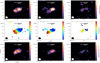 |
Fig. 4 Moment maps of the detected c-C3H2 lines. Peak intensity (top row), intensity-weighted velocity (center row), and integrated intensity (bottom row) maps. The left column shows the images of the C3H2 transition at 217.822 GHz, the middle column for 217.94 GHz, and the right column for 218.16 GHz. The linear size is the same for all maps. The beam is represented as a filled ellipse in the bottom left corner. The green contours represent the disk continuum emission with 10, 150, and 200 times the rms given in Table 1. The white contours represent the molecular emission at 3, 5, and 7 times the rms which is for the moment 0 maps 1σ = 1.7 mJy beam–1 km s–1 (217.82 GHz), 1σ = 1.7 mJy beam–1 km s–1 (217.94 GHz), and 1σ = 0.9 mJy beam-1 km s–1 (218.16 GHz) and for the moment 8 maps 1σ = 0.6 mJy beam–1 (217.82 GHz), 1σ = 0.5 mJy beam–1 (217.94 GHz), and 1σ = 0.5 mJy beam-1 (218.16 GHz). |
3.4.2 13CO
The 13CO (2–1) emission line, an optically thinner line due to its lower abundance than the 12CO (2–1) line, is detected at a peak signal-to-noise (S/N) of 10. The velocity channel maps of the 13CO (2–1) emission line are presented in Fig. A.2. The blueshifted emission is found at velocities between –0.66 and 2.18 km s–1, and it is stronger west of the central protostar. The redshifted emission is much fainter and found mainly east of the protostar. It spans velocities between 4.35 km s–1 and 6.19 km s–1.
Two different faint structures are observed in the channel maps that trace the base of the northeast and southwest components of the molecular outflow and a gaseous disk-like structure surrounding the central protostar. The emission associated with the molecular outflow is only detectable between velocities of 0.35 and 2.35 km s–1. The disk-like structure is detected between –0.66 and 2.18 km s–1 (blueshifted component) and between 4.35 and 6.19 km s–1 (redshifted component) velocities. The blueshifted component is more intense than the redshifted one. We plot the position-velocity diagram (PV) in Fig. 7 to distinguish between redshifted emission associated with the cloud or disk. Although it is a very faint emission, it is compatible with a rotating disk, and we discuss it further in Sect. 4.1.
3.4.3 C18O
The C18O (2–1) emission line is often considered to be optically thin and traces envelopes and disks, although it is only sometimes optically thick (e.g., van ’t Hoff et al. 2018). Blueshifted emission is detected at velocities ranging from 0.01 to 2.68 km s–1 (see Fig. A.3). Redshifted emission spans velocities between 3.02 and 5.18 km s–1. The size of the emission traced by the C18O (2–1) emission above the 5σ contour is 273 ×0793, with a position angle similar to 109° of the dust disk.
In GSS30 IRS3, C18O (2–1) clearly traces a disk-like structure with an obvious redshifted and blueshifted pattern that is compatible with a disk in Keplerian rotation (Fig. 3). When we studied the velocity map, we noted a weak S-shape close to the systemic velocity (Fig. 8). Its nature is discussed in Sect. 5.3.
The spectrum of C18O (2–1) shows a double-peak profile that is typical of an inclined disk in Keplerian rotation.
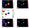 |
Fig. 5 Moment maps of the detected H2CO lines. Peak intensity (top row), intensity-weighted velocity (center row), and integrated intensity (bottom row) maps. The left column shows the images of the H2CO transition at 218.22 GHz, and the right column for 218.47 GHz. There is no intensity-weighted velocity map for 218.47 GHz transition because the emission is only located at 0.7 km s–1. The linear size is the same for all maps. The beam is represented as a filled ellipse in the bottom left corner. The green contours represent the disk continuum emission with 10, 150, and 200 times the rms given in Table 1. White contours represent the molecular emission at 3, 5, and 7 times the rms which is for the moment 0 maps 1σ = 1.5 mJy beam–1 km s–1 (218.22 GHz), and 1σ = 1.0 mJy beam–1 km s–1 (218.47 GHz), and 1σ = 1.0 mJy beam-1 both moment 8 maps. |
3.4.4 c-C3H2
In Class 0 sources, c-C3H2 is usually located in the outflow cavity walls due to exposure to UV radiation from the central protostar (Tychoniec et al. 2021). On the other hand, in Class I sources, hydrocarbons such as c-C3H2 are located in the disk (Tychoniec et al. 2021). We detected the three targeted transitions of c-C3H2 at 217.822 GHz, 217.94 GHz, and 218.160 GHz. The first transition has two blended lines (60,6–51,5 and 61,6–50,5) that are very close (<<m s–1) for the kinematic analysis, and it is more intense than the other two detections (see Fig. 4). c-C3H2 at 217.822 GHz and 217.94 GHz show emission between Vlsr of 0.7 and 4.7 km s–1 , and c-C3H2 at 218.16 GHz is only detected between 0.7 and 3.5 km s–1. In GSS30 IRS3, the c- C3H2 emission is located in the same position as the dust disk (see Fig. 4). The association of the c-C3H2 detection is consistent with both the disk and the disk wind based on its positional information. The kinematics velocities are aligned with a rotation pattern. Therefore, we tentatively attribute the association of c-C3H2 with the disk-like structure.
3.4.5 H2CO
Two out of three transitions are detected, H2CO (30.3–20.2) and H2CO (32,2–22,1). The transition H2CO (30,3–20,2) at 218.22 GHz seems to be located in the same position as the external part of the dust disk and also exhibits a rotation pattern (Fig. 5). H2CO (30,3–20,2) emission is detected at Vlsr values of 0.7 and 4.7 km s–1. The transition H2CO (32,2–22,1) is tentatively detected at the 3σ level in one channel at a Vlsr of 0.7 km s–1.
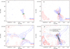 |
Fig. 6 12CO (2–1) integrated emission maps (moment zero) at different velocity stages toward GSS30 IRS3. The green contours represent the dust disk in all the images. The blue contours show blueshifted emission and the red contours show redshifted emission. Panels (a–c) show 3, 5, 7, 9, 11, 13, and 15 times the rms of the respective moment 0 map. (a) Image of the inner high-velocity and narrow outflow component. (b) Close-up image of the hourglass-shape intermediate-velocity component of the molecular outflow. (c) Outer wide-angle low-velocity outflow emission. (d) Combination of panels (a) (dashed with orange and cyan colors), (b) solid, and (c) dotted using 3 and 7 times the rms. The gray image represents the inner high-velocity and narrow outflow. The local standard of rest velocity of the cloud is ∼2.84 km s–1. |
4 Analysis
4.1 Disk rotation
The C18O (2–1) emission line traces a disk-like structure exhibiting indications of rotation (Sect. 3.4.3). It is important to investigate the nature of the rotation, in particularly, whether it is Keplerian. If it is Keplerian rotation, the dynamical mass of the central star can be derived. In order to investigate the rotation curve of the C18O (2–1) emission, we used a PV diagram. The C18O (2–1) line is the most suitable tracer for this analysis because the disk-like structure is clearly detected with a good S/N. This is consistent with being optically thinner than the 13CO (2–1) line, which partially traces the gaseous disk in GSS30 IRS3. In any case, we analyzed the rotation curve of both molecular transitions to compare the obtained results. To compute the PV diagram, we used a cut of 0717 width, which corresponds to the size of the major axis of the synthesized beam, along the major axis of the C18O (2–1) and 13CO (2–1) disk. We adopted a disk position angle value of 109o estimated in Sect. 3.1.
The code SLAM1 (Aso & Sai 2023, Spectral Line Analy- sis/Modeling) was used to analyze the rotation curve of GSS30 IRS3. The process is based on two main steps. The first step is to obtain a 1D intensity profile to derive the edge and ridge data points. The ridge points are defined as the intensity-weighted mean position or the center in the 1-D intensity profile from the Gaussian fitting. The edge points or radius is the outermost position at a certain S/N level. The second step is fitting a power-law (single or double) function that is defined as a positive value to the derived representative data as a function of velocity or radius using the Markov chain Monte Carlo method. Whether it is a function of radius or velocity depends on along which axis the 1D profile for ridge or edge calculations is obtained (see Aso & Sai 2023 criteria for using the vi-ri data points as a function of radius or velocity). The edge and ridge data points were fit independently. Thus, the double power law implies two components with different rotation laws, such as a Keplerian disk and an infalling envelope conserving its specific angular momentum, where the break radius (rb) is the boundary radius between a Keplerian disk and a rotation/infalling envelope, and where the break velocity (υb) is the velocity at rb. We also derived the reduced chi-squared (χ2) for each fit in order to compare all the results. A more detailed explanation of the SLAM method for the eDisk papers can be found in Ohashi et al. (2023).
The code SLAM can fit the systemic velocity as a free parameter. We ran a first test to derive the systemic velocity as 2.84 km s−1 for the C18O (2−1) emission, then we checked this value with the C18O (2−1) spectra and fixed this value for the following test until we derived the final dynamical mass.
We tested a single-power law (bottom left panel in Fig. 7) and double-power law fit (bottom right panel in Fig. 7) to the C18O (2−1) PV diagram. The single power-law fittings give power-law indices (pin) of ~0.71 ± 0.03 for the edge method and ~0.65±0.02 for the ridge method as shown in Table 3. These values are between 0.5 (Keplerian rotation) and 1 (constant specific angular momentum), suggesting that the observed rotation may not be explained by Keplerian rotation alone and may also include rotation in an infalling envelope. To investigate this possibility, double power-law fittings were also performed. The fitting results with the edge method give a pin of ~0.45±0.08 and dp is the difference of the index between the inner and outer parts, that is, ~0.65±0.15 with rb of  au, as shown in Table 4, meaning that the pin for the outside of rb is ~1.1 These results suggest that the observed rotation may be explained as a combination of Keplerian rotation and rotation conserving its specific angular momentum. This type of transition of the rotation between a Keplerian disk and an infalling envelope was observed before in some other protostars as well (e.g., Ohashi et al. 2014; Aso et al. 2015, 2017; Sai et al. 2020). The ridge method did not converge using pin as a free parameter, and we therefore fixed it at 0.5 under the assumption that there is a Kep-lerian disk and we derived a mass of 0.26 ± 0.07 M⊙. Then, the mass derived from the single power-law fit is 0.27 ± 0.07 M⊙ and 0.35 ± 0.09 M⊙ for the double power-law fit as the average of the ridge and edge methods because the edge and the ridge methods over- and underestimate the stellar mass by a factor that depends on the resolution (Maret et al. 2020).
For the 13CO (2−1) line, we only considered the blueshifted component of the emission for the fit, since the redshifted component is very faint. The single-power law fit (top left panel in Fig. 7) shows a lower value of pin than the C18O (2−1) single-power fit. The double power-law fitting did not converge. The single-power fit returned a mass at the break radius (Mb) of 0.24 ± 0.01 M⊙. The edge method results were discarded because we did not obtain stable solutions after several iterations. Additional details about the fitting are described in Appendix D.
The best ;χ2, ignoring the value of ridge double-power law because pin was fixed, was obtained from the C18O (2−1) single-power fit ridge method, but pin is not close to the expected value of a Keplerian disk, and we therefore discarded this value. Then, the second-best χ2 value was obtained from the C18 O (2−1) edge double-power law fit. Therefore, we adopted a mass of GSS30 IRS3 of 0.35±0.09 M⊙.
 |
Fig. 7 13CO (2−1) and C18O (2−1) position velocity diagrams. The top panel show 13CO (2−1) and the bottom panels show C18O (2−1). All the diagrams were obtained along the disk major axis with a position angle of 109 degrees (estimated from the 2D Gaussian fitting) and a width of 0/17. The circles represent the ridge component, and the triangles show the edge component using SLAM. The solid and dashed curves represent fitting results obtained with the ridge and edge methods, respectively. The different colors show data points obtained along different directions. The cyan and magenta points represent data points obtained along the velocity axis, and blue and red show data points obtained along the position axis. The lime contours mark the emission at 3, 6, and 9 times the rms given in Table 2. Further details of the fitting procedure can be found in Aso & Sai (2023). The left column shows the single power-law fit, and the right column shows the double power law fit. |
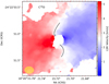 |
Fig. 8 Zoom-in image of the velocity map of C18O (2−1). The S-shape is overplotted by hand in black. The innermost white region does not show the systemic velocity. |
Results from the SLAM fitting to the position velocity diagram using a single power law.
Results from the SLAM fitting to the position velocity diagram using a double powerlaw.
4.2 Characterization of the molecular outflow
In this subsection, we analyze the three different components of the molecular outflow described in Sect. 3.4.1 in more detail.
The most collimated inner high-velocity outflow component is extended to a maximum deprojected length of 2″.3 (1.5×10⁻³pc). The maximum deprojected extension of the intermediate-velocity component with an hourglass shape is 3″.3, and the maximum deprojected length of the wider-angle lower-velocity component is 8″.3 and 2″.7 for the northeast and southwest arc-like structures, respectively. The size of the different components was measured using a bisecting line from the center of the disk continuum emission to the maximum extension of each component, considering the 5σ contour.
The most collimated inner high-velocity outflow component exhibits an opening angle of ~34 degrees. On the other hand, the intermediate-velocity component with an hourglass shape shows an opening angle of ~70 degrees. For the wider-angle low-velocity outflow component, we estimate values of ~ 120 degrees and ~100 degrees for the northeastern and southwestern lobes, respectively. These values were measured by hand using a protractor over the flux-integrated map (Fig. 6). Table 5 summarizes all these values.
Given that our observations were not designed or optimized for studying extended molecular outflows and that we likely filtered out structures larger than ~2″.0, we derived the dynamical parameters of the outflow as a first characterization in Appendix E. The results in Table 6 must be considered with caution, however, and they are only valid for the most compact emission of the outflow.
5 Discussion
5.1 Asymmetric intensity distribution along the minor axis of the dust disk
The eDisk results showed an asymmetric intensity distribution along the disk minor axis in several sources (e.g., Ohashi et al. 2023; Takakuwa et al. 2024; Lin et al. 2023; Sai et al. 2023; Kido et al. 2023a; van’t Hoff et al. 2023; Gavino et al. 2024; Han et al., in prep.). The asymmetries found in the minor axes in these eDisk subsample are generally explained as due to a combination of optically thick emission and disk flaring, as proved in the radiative transfer studies of Lin et al. (2023) and Takakuwa et al. (2024). As a result, dust is not settled onto the midplane, but is distributed vertically, which can in some cases create a dark lane. This dark lane observed in edge-on disks has been described as a hamburger shape (Lee et al. 2017; Galván-Madrid et al. 2018).
In the case of the orientation of the GSS30 IRS3 disk, the northeastern region corresponds to the far side of the disk. This conclusion is based on the peak intensity position, which exhibits a slight skew from the geometric center and toward the northeast, as determined by fitting an ellipse to a 5σ contour level.
Moreover, this is supported by the orientation of the collimated high-velocity molecular outflow, where the blueshifted emission points toward the northeast. This alignment provides a rationale for the observed brightness asymmetry in the minor axis between the two sides of the disk. Additionally, the boxy dust disk shape (Fig. 1) might be explained as the truncated edge of a flared disk.
Consequently, the asymmetry in the minor axis can be attributed to a combination of disk flaring and optically thick emission.
Geometric parameters of the three molecular outflow components (northeast and southwest component) deprojected for an inclination of 64.3°.
Inclination-corrected dynamical properties of the blue- and redshifted emission of the three molecular outflow components.
5.2 Origin of the bumps along the major axis
A subset of eDisk sources reported a brightness asymmetry or bumps along the major axis of the protostellar disks (Sai et al. 2023; van’t Hoff et al. 2023; Kido et al. 2023b). In the case of GSS30 IRS3, two bumps are detected along the disk major axis. To confirm the authenticity of the bumps and eliminate the possibility that they are spurious artifacts from the cleaning process, we fit the radial intensity profile in the uv plane using Frank (see Appendix F). Frank (Jennings et al. 2020) first depro-jected the visibilities to correct for the disk inclination and used the Fourier-Bessel series to reconstruct the radial brightness profile. One bump is located at a radius of ~0″.19 (~26 au) and the other is located at ~0″.36 (~50 au) from the center of the disk. The positions of the identified bumps closely coincide with those obtained from the radial intensity profile in the image plane. This alignment strongly rules out the possibility that they are artifacts. However, we emphasize that our interpretation is only limited to discarding spurious signals in the cleaning process given the Frank limitations when dealing with a flared disk.
We discuss the main two possible explanations for the origin of the bumps. First, there could be a real substructure within the dusty disk that will likely evolve into a more well-defined structure over time. Alternatively, the bumps might be the result of the temperature distribution caused by the optically thick continuum emission. To test the second possibility, we compared the dust brightness temperatures at the bump locations with the expected midplane temperature at the same location in a passively heated and flared disk.
To obtain the midplane temperature (Tmid), we employed the equation Tmid(r) = (ϕ L*/8πr2σSB)0.25 (Chiang & Goldreich 1997; D’Alessio et al. 1998; Dullemond et al. 2001), where r is the radius (0″.19 and 0″.36), σSB denotes the Stefan-Boltzmann constant, L* is the bolometric luminosity of the central protostar (1.7 L⊙), and ϕ corresponds to the assumed flaring angle of 0.02 radian (Huang et al. 2018). The predicted midplane temperature is 27.8 K at a radius of 0.’ 19 and 20.2 K at a radius of 0″.36. However, the observed brightness temperature at 0″.19 and 0″.36 is 18.9 and 9.6 K, respectively. The observed brightness distribution along the major axis of the disk is compared with the estimated midplane temperature distribution in Fig. 9, which shows that the observed brightness temperature is lower than the estimated midplane temperature. This suggests that the 1.3 mm continuum emission is not completely optically thick, as we would expect the observed brightness temperature to be similar to the actual physical temperature. It is, however, advisable to exercise caution in interpreting the observed brightness temperature distribution as an accurate representation of the actual radial brightness temperature distribution of the disk because the disk is inclined at a significant angle, which introduces a number of complications. In an edge-on disk, the brightness temperature is measured at a point where the optical depth along the line of sight becomes unity. Consequently, the distance of the measurement point from the center is not necessarily equivalent to the corresponding project distance from the center.
Future continuum observations at lower frequencies with ALMA that trace optically thinner dust emission could help to validate our findings. A more detailed radiative transfer modeling, which is beyond the scope of this paper, might also further elucidate the true nature of these bumps and their relation with the substructures observed in more evolved sources.
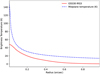 |
Fig. 9 Azimuthal brightness distribution vs. the radius for GSS30 IRS3 (continuous red line) and the theoretical midplane temperature (dashed blue line). |
5.3 Kinematics and the origin of the S-shape in the C18O line emission
In this subsection, we discuss the origin of the twisted feature observed in the C18O (2−1) velocity map (Sect. 3.4.3). Similar S-shape or twisted velocity maps close to the systemic velocity are usually associated with warped disks in young stellar objects (Rosenfeld et al. 2012; Facchini et al. 2018; Zhu 2019). The origin of these features has several possible explanations: A misaligned binary (Terquem & Bertout 1993; Papaloizou & Terquem 1995; Fragner & Nelson 2010; Nixon et al. 2013; Facchini et al. 2018), a fast radial infall attributed to the presence of a giant planet, brown dwarf, or low-mass companion (Rosenfeld et al. 2014), the effect of a stellar fly-by (Dai et al. 2015; Kurtovic et al. 2018; Cuello et al. 2019), or the transition from a Keplerian disk to an infalling envelope (Aso et al. 2015; Sai et al. 2020). The first two theories are usually applied to more evolved young stellar objects.
The eDisk sample contains another source with a twisted kinematic map (Flores et al. 2023, Oph IRS63). The C18O (2−1) and SO (6−5) moment 1 maps showed an S-shaped feature that is explained by infalling motion. In the case of GSS30 IRS3 observations, we also detected an infalling envelope, according to the double-power law fit from SLAM (see Sect. 4.1) Although the most likely explanation is an infalling envelope onto the disk, the twisted kinematic feature alone does not provide sufficient evidence for further analysis. On the other hand, we are unable to confirm that the origin of the S-shape is an undetected close binary (within ~8 au) or an embedded companion. We do not observe indications of a recent star flyby either. Future modeling, incorporating hydrodynamic simulations, may be able to explain the origin of the S-shape. Modeling like this is beyond the scope of this initial analysis.
5.4 Coexistence of a jet and a wide-angle outflow
Accretion and ejection are fundamental processes in star formation. They shape the evolution of young stars and their environment. The relation between ejection and accretion processes is not completely understood, but the accretion of gas and dust that fall from the inner edge of the protoplanetary disk onto the young stellar object drives the ejection of material. Ejection of material removes the excess of angular momentum through two different types of structures: a collimated component at high velocity, and a wider-angle component at lower velocities. The collimated component or jet propagates into the surrounding molecular cloud, forming bow shocks that push the gas and produce outflow shells in the jet vicinity (Raga & Cabrit 1993). Different knots are usually detected along the jet direction as a signal of episodic material ejection. On the other hand, the wide-angle component is a radial disk wind that blows the ambient cloud, forming expanding shells (Li & Shu 1996; Lee et al. 2000). Therefore, the jet and wind angle disk-driven structures are able to explain the mass-loss process in star formation with different theories. Interestingly, Rabenanahary et al. (2022) presented simulations demonstrating that jet and wide-angle disk-wind-driven ejections could coexist, and we therefore expect the simultaneous detection of collimated and wide-angle outflow components during the early stages of star formation.
The 12CO observations of GSS30 IRS3 reveal three distinct components: a collimated outflow whose axis is aligned with several knots seen in molecular hydrogen (Fig. B.1), a conical hourglass shape, and a wide-angle low-velocity component with a parabolic morphology (Fig. 6). The analysis of the conical outflow described in Sect. 3.4.1 suggests that it is produced by a jet. While the blueshifted lobe of the wider angle outflow clearly exhibits emission shifting away from the central object as velocity increases, this is consistent with the predictions of the wind-driven shell model (Lee et al. 2000).
The coexistence of collimated jets/outflows and slow wider-angle molecular outflows has previously been detected in young protostars at early stages, specifically, in two Class I sources in HH 46/47 (Zhang et al. 2019) and DG Tauri B (de Valon et al. 2020, 2022) or more recently in several sources (Federman et al. 2024). Compared with these sources, GSS30 IRS3 exhibits very distinguishable components, even with observations that were not initially designed to study molecular outflows. Moreover, this is one of the few sources in which the coexistence of a jet and a wide-angle outflow has clearly been detected in a young Class 0 protostar in the submillimeter regime, making this source one of the best objects for future detailed studies of the accretion-ejection processes in the early stages of star formation.
6 Conclusions
We presented high-resolution ALMA observations at 1.3 mm of the Class 0 protostar GSS30 IRS3, conducted as part of the eDisk ALMA program at a spatial resolution of ~8 au. Our observations targeted the continuum emission as well as several molecular species, including 12CO (2−1), 13CO (2−1), C18O (2−1), and c-C3H2 (blended lines 60,6-51,5 and 61,6−50,5 217.822 GHz), c-C3H2 (51,4−42,3 217.940 GHz), c-C3H2 (52,4−41,3 218.16 GHz), H2CO (30,3−20,2 218.22 GHz), andH2CO (32,2−22,1 218.47 GHz). We summarize our findings below.
1. We detected dust continuum emission that traced a disklike structure. The dust disk size is 1″.43 × 0″.62 (~198 × ~86 au) with an inclination of 64.3 ± 1.5o and a position angle of 109o. The mass of the dust disk in GSS30 IRS3 is estimated to range between 23.87 ± 0.90 M⊕ and 75.1 ± 2.9 M⊕ depending on the adopted Tdust.
2. The dust disk of GSS30 IRS3 does not exhibit clear substructures such as spirals. We report an asymmetry in the minor axis that can be attributed to an optically thick emission and disk flaring. Additionally, we note the detection of two bumps located at 26 au and 50 au from the disk center along the major axis. The origin of these bumps remains unclear, and we propose two main hypotheses: they might indicate embedded real substructures within the disk, or we might trace the temperature distribution.
3. The C18O (2−1) emission traces a Keplerian disk and the infalling rotating envelope, allowing us to derive a dynamic mass of 0.35±0.09 M⊙ of the central protostar with a disk gas size radius between 47 and 107 au.
4. Our 12CO (2−1) high-resolution and sensitive observations revealed the coexistence of a jet and a wide-angle outflow.
Acknowledgements
We thank the referee, Tien-Hao Hsieh, for the helpful comments and suggestions on this manuscript. We would like to thank all the ALMA staff supporting this work. This paper makes use of the following ALMA data: ADS/JAO.ALMA#2019.1.00261.L, 2019.A.00034.S ALMA is a partnership of ESO (representing its member states), NSF (USA) and NINS (Japan), together with NRC (Canada), MOST and ASIAA (Taiwan), and KASI (Republic of Korea), in cooperation with the Republic of Chile. The Joint ALMA Observatory is operated by ESO, AUI/NRAO and NAOJ. J.J.T. acknowledges support from NASA XRP 80NSSC22K1159. The National Radio Astronomy Observatory is a facility of the National Science Foundation operated under cooperative agreement by Associated Universities, Inc. N.O. acknowledges support from National Science and Technology Council (NSTC) in Taiwan through the grants NSTC 109-2112-M-001-051, 110-2112-M-001-031, 110-2124-M-001-007, and 111-2124-M-001-005. J.K.J. acknowledges support from the Independent Research Fund Denmark (grant No. 0135-00123B). C.W.L. is supported by the Basic Science Research Program through the National Research Foundation of Korea (NRF) funded by the Ministry of Education, Science and Technology (NRF-2019R1A2C1010851), and by the Korea Astronomy and Space Science Institute grant funded by the Korea government (MSIT; Project No. 2022-1-840-05). Z.-Y.L. is supported in part by NASA NSSC20K0533 and NSF AST-2307199 and AST-1910106. L.W.L. acknowledges support from NSF AST-2108794. J.P.W. acknowledges support from NSF AST-2107841. W.K. was supported by the National Research Foundation of Korea (NRF) grant funded by the Korea government (MSIT) (RS-2024-00342488). ZYDL acknowledges support from NASA 80NSSCK1095, the Jefferson Scholars Foundation, the NRAO ALMA Student Observing Support (SOS) SOSPA8-003, the Achievements Rewards for College Scientists (ARCS) Foundation Washington Chapter, the Virginia Space Grant Consortium (VSGC), and UVA research computing (RIVANNA). S.T. is supported by JSPS KAKENHI grant Nos. 21H00048 and 21H04495, and by NAOJ ALMA Scientific Research grant No. 2022-20A. H.-W.Y. acknowledges support from the National Science and Technology Council (NSTC) in Taiwan through the grant NSTC 110-2628-M-001-003-MY3 and from the Academia Sinica Career Development Award (AS-CDA-111-M03). IdG acknowledges support from grant PID2020-114461GB-I00, funded by MCIN/AEI/10.13039/501100011033. ASM thanks Laura Pérez and Anibal Sierra for their valuable help and insights on using the Frank.
Appendix A Channel maps
This section shows the channel maps for 12CO (Sect. 3.4.1), 13CO (Sect. 3.4.2), and C18O (Sect. 3.4.3)
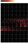 |
Fig. A.1 Channel maps of the 12CO (2−1) emission in GSS30 IRS3. Emission is detected above 5σ from −19.9 km s−1 to 23.8 km s−1. The color scale is stretched using the inverse hyperbolic sine function. The lowest contour emission corresponds to 5σ (1σ corresponds to 1.00 mJy beam−1), with increments of 10σ. The field of view of the map is 12″ × 12″. |
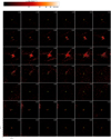 |
Fig. A.2 Channel maps of the 13CO (2−1) emission in GSS30 IRS3. Emission is detected above 5σ from −0.66 km s−1 to 6.19 km s−1. The color scale is stretched using the inverse hyperbolic sine function. The lowest contour emission corresponds to 5σ (1σ corresponds to 2.10 mJy beam−1), with increments of 10σ. The field of view of the map is 8″ × 8″. |
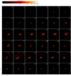 |
Fig. A.3 Channel maps of the C18O (2−1) emission in GSS30 IRS3. Emission is detected above 5σ from −0.66 km s−1 to 5.19 km s−1. The color scale is stretched using the inverse hyperbolic sine function. The lowest contour emission corresponds to 5σ (1σ corresponds to 1.83 mJy beam−1), with increments of 10σ. The field of view of the map is 6″ × 6″. |
Appendix B JWST images
We compare the image of the 12CO molecular outflow with recent JWST images obtained with NIRCAM (PI K. Pontoppi-dan) centered over GSS30 IRS3.
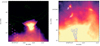 |
Fig. B.1 JWST molecular hydrogen color image (4.7 µm image with the F470N filter) over GSS30 IRS3 (12CO). Left panel shows the blueshifted component from the bottom-left panel of Fig. 6 with contours over 3 times the rms. Right panel only shows the collimated blueshifted and redshifted molecular outflow. Color image contrast limits are adjusted to enhance the presence of two knots in the direction of the blueshifted collimated molecular outflow emission which are pointed with two white arrows. The knots are located at 4″.9 and 6″.7 from the center of the continuum emission. Contours represent 3, 5, 7, 9, 11, 13 and 15 times the rms. |
Appendix C Other sources detected in the field of view
C.1 GSS30 IRS 1
We report the continuum detection of GSS30 IRS1, a Class I young stellar object (Michel et al. 2023), located at a distance of approximately 14.7 arcseconds from GSS30 IRS3. Figure C.1 shows the 1.3 mm dust emission from GSS30 IRS1 with an angular resolution of 0″.052×0″.042 (position angle of 2.5o), obtained using a robust parameter equal to 0.5. The continuum emission traces an inclined disk-like structure around the central protostar, with a small appendix similar to a spiral-like structure located at the west-south of the disk. The continuum emission measured above a 5σ contour for the disk-like structure (excluding the spiral-like structure) has major and minor axes of 0″.34×0″.22 (~67 × ~44 au), with a peak intensity and flux density of 2.72 mJy beam−1 and 3.92 mJy, respectively. Coordinate of the peak intensity is RA=16h26m21.354s, Dec= −24o 23’05″.03. The rms is 17.1 µJy beam s−1. The inclination derived from the disk-like structure is approximately 50°.
Several emission lines, including 12CO (2−1), 13CO (2−1), C18O (2−1), SO (65−54), and SiO (5−4), were detected surrounding GSS30 IRS1. A detailed analysis of the gas source and the spiral-like structure will be presented in a follow-up paper (Santamaría-Miranda et al. in prep).
C.2 GSS30 IRS2
We report the detection of gas material surrounding the Weak-line T-Tauri star (Dolidze & Arakelyan 1959) GSS 30 IRS2 that is classified as M2 spectral type (Greene & Meyer 1995). The 12CO emission is detected between −2.2 km s−1 and 1.6 km s−1 with respect to the local standard of velocity rest, and it integrated map is shown in Fig. C.2. Redshifted emission is very contaminated by cloud emission, and it is impossible to distinguish between emission from the source and from the cloud. The emission size is r″.3×0″.8 based on the 5σ contour. There is not also very clear molecular outflow emission. Furthermore, there is no clear rotation in the intensity-weighted velocity map (right panel in Fig. C.2). There is no detection of the continuum at 3σ level (5.2 µJy beam−1) or any other of the emission lines. A summary of the main properties is shown in Table C.1.
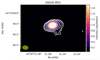 |
Fig. C.1 ALMA continuum image of GSS3O IRS1 at 1.3 mm. White contours are 5, 10, 20, 40, 60, 80, 100, and 130 times the rms (1σ = 17.1 µJy beam−1). |
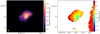 |
Fig. C.2 GSS3O IRS2 moments maps. Left panel: 12CO emission line flux-integrated map. White contours represent the 3, 5, 7, 9, 11, 13, 15 times the rms that is 8.8 mJy beam−1 km s−1. Yellow cross represents the position of the central source. Right panel: 12CO (2−1) emission line intensity-weighted velocity map of GSS3O IRS2. |
Appendix D SLAM fitting
This section shows the result of corner plot (Figs. D.1 and D.2) of the SLAM fitting in Sect. 4.1 for the C18O and 13CO lines.
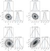 |
Fig. D.1 Corner plot of the SLAM fitting using single-power law fitting. Top and bottom panels show the results for the C18O (2−1) and 13CO (2−1) emission, and the left and right panels those with the edge and ridge methods, respectively. Dashed lines are the 16 and 84 percentiles. These plots shows that the prior ranges are wide enough to constrain the fitting parameters. |
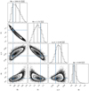 |
Fig. D.2 Corner plot of the SLAM double-power law fitting for the C18O (2−1) line using the edge method. Dashed lines are the 16 and 84 percentiles. |
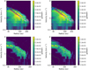 |
Fig. D.3 Position velocity diagrams of the SLAM fitting in logarithm scale. Top and bottom panels show the results for the C18O (2−1) and 13CO (2−1) emission, and the left and right panels those with single- and double-power law fitting, respectively. Symbols and colors are as shown in Fig. 7. |
Appendix E Dynamical parameters of the molecular outflow components
Here we analyze the dynamic properties of the three different components of the molecular outflow, separated in blueshited and redshifted emission with respect to the systemic velocity (2.84 km s−1, as inferred in Sect. 4.1). We will consider the emission inside the 3σ contour level in Fig. 6 to perform the calculation in this subsection. For inferring the dynamical properties of the molecular outflow, we will consider the 12CO (2−1) molecular line since this transition clearly traces the different components of the outflow with good S/N, and the13 CO (2−1) line traces only the outflowing material closer to the central protostar together with a rotating disk. We calculate the dynamical time, the outflow mass, the mass-loss rate, the outflow momentum, the kinetic energy, the mechanical luminosity, and the outflow force.
The dynamical time of the various outflow components was determined by considering the deprojected maximum velocity, the deprojected length, and an outflow axis perpendicular to the dust disk, whose inclination is derived in Sect. 3.1.
The maximum inferred dynamical time is approximately 535 years for the wider angle lower velocity blueshifted component. When considering both the blueshifted and redshifted emission, the average dynamical time for this component is around 340 years. We used the maximum velocity to calculate the dynamical time of each of the components. Then we averaged the dynamical time between the blue and red component. The intermediate velocity hourglass shape component exhibits an average dynamical time of approximately 43 years when considering both blueshifted and redshifted emission. Similarly, the most collimated inner high-velocity component shows an average dynamical time of approximately 31 years.
The 12CO (2−1) emission line is optically thick at systemic velocities, since the brightness temperature of the line peak 57.9 K is similar to the kinetic temperature that we measured (58.7 K) from the linewidth. Therefore we determine the excitation temperature for the 12CO (2−1) line using the peak intensity obtained close to the position of the star as
![Mathematical equation: ${T_{{\rm{ex}}}} = {{h{v_{12}}/k} \over {\ln \left[ {1 + {{h{v_{12}}/k} \over {{T_{o12}} + {J_{12}}(2.7K)}}} \right]}},$](/articles/aa/full_html/2024/10/aa49981-24/aa49981-24-eq7.png) (E.1)
(E.1)
where T0 is the peak brightness temperature obtained close to the central continuum peak position. We derived a Tex for the 12CO (2−1) of 25.7 K, and we assumed this value for all the molecular outflow components.
Then, we followed the prescription in Scoville et al. (1986) and Palau et al. (2007) to calculate the column density and the mass of the outflow. We derived the mean optical depth in the wings of the 12CO (2−1) emission line. We define the line wings as [−19.9 km s−1, −18,7 km s−1] and [23.2 km s−1, 23.8 km s−1] for the inner molecular outflow, [−18.0 km s−1, −17.4 km s−1] and [21.9 km s−1, 22.6 km s−1] for the intermediate hourglass shape and only two channels (−1.6 km s−1 and 7.9 km s−1) for the wider angle low velocity molecular outflow. The optical depth is obtained for each of the three molecular outflow components, obtaining values between 0.04 and 0.51, in the optically thin regime. Then we assume that the emission is optically thin in the line wings. We infer a column density ~2×1016cm2 for the wider angle and the inner molecular outflow components and a value one order of magnitude smaller for the highly collimated high-velocity molecular outflow component. Finally, we calculated the outflow mass using the inferred column density, the emission area, and a CO abundance of 10−4.
GSS30 IRS2 main properties in the 12CO (2−1) emission line
We derived the rest of the parameters following the formulas in Santamaría-Miranda et al. (2020, Table 3) correcting for inclination. The total outflow mass of the molecular outflow is 6.1×10⁻⁵ M⊙, the momentum varies between 9.8×10⁻⁶ M⊙ km s−1 and 4.5×10⁻³ M⊙ km s−1, the kinetic energy varies between 4.7 ×1039 erg and 4.7 ×1041 erg, and the mechanical force varies between 4.8×10⁻⁷ M⊙ km s−1 yr−1 and 1.0×10⁻⁵ M⊙ km s−1 yr−1 . All these parameters are summarized in Table 6.
These results are affected by several assumptions that may affect the estimated mass. Previous studies point out that the optical depth of molecular outflows is underestimated, and masses should be at least a factor two higher (Dunham et al. 2014) or five (van der Marel et al. 2013). The first source of uncertainty is Tex; our value is in the expected range for molecular outflows (Tex = 10-50 K Bally 2016); if we use a Tex=50 K, the mass will increase by a factor of 1.4 with respect to that with Tex=25.7 K. Another source of uncertainties is related to the parental cloud material that contaminates the emission of the molecular outflow close to the systemic velocity, needing the exclusion of those channels for the dynamical parameters calculations. Offner et al. (2011), using synthetic observations, found that the missed outflow mass might increase by a factor 5 to 10 within 2 km s−1 from the rest velocity. However, the most significant uncertainty factor in our calculations is the interfero-metric filtering. It is noticeable when comparing our dynamical properties with the ones obtained in low-mass Class 0 molecular outflows observed with single-dish telescopes. For example, the outflow mass in Class 0 and I sources is in the range between ×10−3 M⊙ and ×10−1 M⊙ (Mottram et al. 2017), and our total outflow mass is below these values. Another example is the mechanical force expected to be between 1.0×10⁻⁵ M⊙ year−1 km s−1 and ×10−2 M⊙ yr−1 km s−1 for Class 0 sources (Mottram et al. 2017) and the mechanical force of GSS30 IRS3 outflow is in the lower limit. Therefore, we conclude that all derived parameters may be treated as lower limits.
Appendix F Radial brightness profile fitting
To further investigate if the bumps detected in the major axis of the radial intensity profile of the dust disk surrounding GSS30 IRS3 are real features and not a byproduct of the cleaning process, we fit a 1D profile to the ALMA visibilities with a non-parametric model using the Frank library (Jennings et al. 2020), which provides a super-resolution brightness profile reconstruction. A major advantage of fitting visibilities is avoiding false structures created during the CLEAN process. Data were averaged in frequency to get spectral windows of 8 channels to reduce data volume and speed up calculations, excluding baseband 1 and 4, which are dedicated to detecting molecular emission lines or has a strong detected line where the contribution to the continuum was negligible. Frank can estimate the inclination and position angle of the protoplanetary disk; however, Benisty et al. (2021) noted that Frank does not fit these two parameters accurately, so we fixed them to an inclination of 64.30 deg and a position angle of 109 deg, as inferred in Sect. 3.1 considering the emission above the 5σ contour.
Before fitting a Bessel functions to the brightness profile, Frank applies a power spectrum estimate as a prior. There are several hyperparameters that affect this power spectrum, but the two most relevant ones are α and wsmooth. α works as an S/N threshold for the maximum baseline where visibilities are fitted (a higher value implies a stricter S/N threshold), while wsmooth affects the smoothness of the power spectrum, where a higher value implies a smoother power spectrum. We explore the fitting quality using different hyperparameters values (α between 1.05 and 1.30 and wsmooth between 10−4 and 10−1), not finding any substantial difference between the different fittings. We fixed the hyperparameters to α= 1.30 and wsmooth=10−4 because they present the least noisy results. The best-fit model (Fig. F.1) showed the presence of two bumps. To obtain the bumps size and location, we fit an exponential to the brightness profile obtained from Frank to isolate the bumps. Then, we fitted Gaussians around the areas where the bumps are located. Their positions are ~0″.19 (~26 au) and ~0″.36 (~50 au) from the center of the disk, 0″.09 (~13.6 au) and 0″.14 (~19 au) wide, respectively.
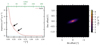 |
Fig. F.1 Results of the best one-dimension Frank fit. The left panel is the fitted radial intensity frank profile. The position of the bumps is marked with two black arrows. The right panel is the non-convolved Frank profile reprojected over two dimensions. |
References
- ALMA Partnership (Brogan, C. L., et al.) 2015, ApJ, 808, L3 [Google Scholar]
- Andrews, S. M., Wilner, D. J., Zhu, Z., et al. 2016, ApJ, 820, L40 [Google Scholar]
- Andrews, S. M., Huang, J., Pérez, L. M., et al. 2018, ApJ, 869, L41 [NASA ADS] [CrossRef] [Google Scholar]
- Aso, Y., & Sai, J. 2023, https://doi.org/10.5281/zenodo.7783868 [Google Scholar]
- Aso, Y., Ohashi, N., Saigo, K., et al. 2015, ApJ, 812, 27 [Google Scholar]
- Aso, Y., Ohashi, N., Aikawa, Y., et al. 2017, ApJ, 849, 56 [NASA ADS] [CrossRef] [Google Scholar]
- Bally, J. 2016, ARA&A, 54, 491 [Google Scholar]
- Beckwith, S. V. W., Sargent, A. I., Chini, R. S., & Guesten, R. 1990, AJ, 99, 924 [Google Scholar]
- Benisty, M., Bae, J., Facchini, S., et al. 2021, ApJ, 916, L2 [NASA ADS] [CrossRef] [Google Scholar]
- Chiang, E. I., & Goldreich, P. 1997, ApJ, 490, 368 [Google Scholar]
- Cieza, L. A., González-Ruilova, C., Hales, A. S., et al. 2021, MNRAS, 501, 2934 [Google Scholar]
- Cuello, N., Dipierro, G., Mentiplay, D., et al. 2019, MNRAS, 483, 4114 [Google Scholar]
- Dai, F., Facchini, S., Clarke, C. J., & Haworth, T. J. 2015, MNRAS, 449, 1996 [Google Scholar]
- D’Alessio, P., Cantö, J., Calvet, N., & Lizano, S. 1998, ApJ, 500, 411 [Google Scholar]
- de Valon, A., Dougados, C., Cabrit, S., et al. 2020, A&A, 634, L12 [NASA ADS] [CrossRef] [EDP Sciences] [Google Scholar]
- de Valon, A., Dougados, C., Cabrit, S., et al. 2022, A&A, 668, A78 [NASA ADS] [CrossRef] [EDP Sciences] [Google Scholar]
- Dolidze, M. V., & Arakelyan, M. A. 1959, Soviet Ast., 3, 434 [NASA ADS] [Google Scholar]
- Dullemond, C. P., Dominik, C., & Natta, A. 2001, ApJ, 560, 957 [NASA ADS] [CrossRef] [Google Scholar]
- Dunham, M. M., Arce, H. G., Mardones, D., et al. 2014, ApJ, 783, 29 [NASA ADS] [CrossRef] [Google Scholar]
- Facchini, S., Juhász, A., & Lodato, G. 2018, MNRAS, 473, 4459 [Google Scholar]
- Federman, S. A., Megeath, S. T., Rubinstein, A. E., et al. 2024, ApJ, 966, 41 [CrossRef] [Google Scholar]
- Flock, M., Ruge, J. P., Dzyurkevich, N., et al. 2015, A&A, 574, A68 [NASA ADS] [CrossRef] [EDP Sciences] [Google Scholar]
- Flores, C., Ohashi, N., Tobin, J. J., et al. 2023, ApJ, 958, 98 [NASA ADS] [CrossRef] [Google Scholar]
- Fragner, M. M., & Nelson, R. P. 2010, A&A, 511, A77 [NASA ADS] [CrossRef] [EDP Sciences] [Google Scholar]
- Friesen, R. K., Pon, A., Bourke, T. L., et al. 2018, ApJ, 869, 158 [NASA ADS] [CrossRef] [Google Scholar]
- Galván-Madrid, R., Liu, H. B., Izquierdo, A. F., et al. 2018, ApJ, 868, 39 [CrossRef] [Google Scholar]
- Gavino, S., Jørgensen, J. K., Sharma, R., et al. 2024, ApJ, accepted [arXiv: 2407.17249] [Google Scholar]
- Greene, T. P., & Meyer, M. R. 1995, ApJ, 450, 233 [NASA ADS] [CrossRef] [Google Scholar]
- Hildebrand, R. H. 1983, QJRAS, 24, 267 [NASA ADS] [Google Scholar]
- Huang, J., Andrews, S. M., Dullemond, C. P., et al. 2018, ApJ, 869, L42 [NASA ADS] [CrossRef] [Google Scholar]
- Jennings, J., Booth, R. A., Tazzari, M., Rosotti, G. P., & Clarke, C. J. 2020, MNRAS, 495, 3209 [Google Scholar]
- Jhan, K.-S., & Lee, C.-F. 2016, ApJ, 816, 32 [NASA ADS] [CrossRef] [Google Scholar]
- Jørgensen, J. K., van Dishoeck, E. F., Visser, R., et al. 2009, A&A, 507, 861 [NASA ADS] [CrossRef] [EDP Sciences] [Google Scholar]
- Kido, M., Takakuwa, S., Saigo, K., et al. 2023a, ApJ, 953, 190 [NASA ADS] [CrossRef] [Google Scholar]
- Kido, M., Takakuwa, S., Saigo, K., et al. 2023b, ApJ, 953, 190 [NASA ADS] [CrossRef] [Google Scholar]
- Kurtovic, N. T., Pérez, L. M., Benisty, M., et al. 2018, ApJ, 869, L44 [Google Scholar]
- Lee, C.-F., Mundy, L. G., Reipurth, B., Ostriker, E. C., & Stone, J. M. 2000, ApJ, 542, 925 [NASA ADS] [CrossRef] [Google Scholar]
- Lee, C.-F., Hirano, N., Zhang, Q., et al. 2015, ApJ, 805, 186 [NASA ADS] [CrossRef] [Google Scholar]
- Lee, C.-F., Li, Z.-Y., Ho, P. T. P., et al. 2017, Sci. Adv., 3, e1602935 [NASA ADS] [CrossRef] [Google Scholar]
- Li, Z.-Y., & Shu, F. H. 1996, ApJ, 472, 211 [NASA ADS] [CrossRef] [Google Scholar]
- Lin, Z.-Y. D., Li, Z.-Y., Tobin, J. J., et al. 2023, ApJ, 951, 9 [NASA ADS] [CrossRef] [Google Scholar]
- Long, F., Pinilla, P., Herczeg, G. J., et al. 2018, ApJ, 869, 17 [Google Scholar]
- Manara, C. F., Morbidelli, A., & Guillot, T. 2018, A&A, 618, L3 [NASA ADS] [CrossRef] [EDP Sciences] [Google Scholar]
- Maret, S., Maury, A. J., Belloche, A., et al. 2020, A&A, 635, A15 [NASA ADS] [CrossRef] [EDP Sciences] [Google Scholar]
- McMullin, J. P., Waters, B., Schiebel, D., Young, W., & Golap, K. 2007, ASP Conf. Ser., 376, 127 [Google Scholar]
- Michel, A., Sadavoy, S. I., Sheehan, P. D., et al. 2023, AJ, 166, 184 [NASA ADS] [CrossRef] [Google Scholar]
- Mottram, J. C., van Dishoeck, E. F., Kristensen, L. E., et al. 2017, A&A, 600, A99 [NASA ADS] [CrossRef] [EDP Sciences] [Google Scholar]
- Nixon, C., King, A., & Price, D. 2013, MNRAS, 434, 1946 [NASA ADS] [CrossRef] [Google Scholar]
- Offner, S. S. R., Lee, E. J., Goodman, A. A., & Arce, H. 2011, ApJ, 743, 91 [CrossRef] [Google Scholar]
- Ohashi, N., Saigo, K., Aso, Y., et al. 2014, ApJ, 796, 131 [NASA ADS] [CrossRef] [Google Scholar]
- Ohashi, N., Tobin, J. J., Jørgensen, J. K., et al. 2023, ApJ, 951, 8 [NASA ADS] [CrossRef] [Google Scholar]
- Ortiz-León, G. N., Loinard, L., Dzib, S. A., et al. 2018, ApJ, 869, L33 [Google Scholar]
- Palau, A., Estalella, R., Ho, P. T. P., Beuther, H., & Beltrán, M. T. 2007, A&A, 474, 911 [NASA ADS] [CrossRef] [EDP Sciences] [Google Scholar]
- Papaloizou, J. C. B., & Terquem, C. 1995, MNRAS, 274, 987 [NASA ADS] [Google Scholar]
- Pascucci, I., Testi, L., Herczeg, G. J., et al. 2016, ApJ, 831, 125 [Google Scholar]
- Podio, L., Codella, C., Gueth, F., et al. 2016, A&A, 593, L4 [NASA ADS] [CrossRef] [EDP Sciences] [Google Scholar]
- Rabenanahary, M., Cabrit, S., Meliani, Z., & Pineau des Forêts, G. 2022, A&A, 664, A118 [NASA ADS] [CrossRef] [EDP Sciences] [Google Scholar]
- Raga, A., & Cabrit, S. 1993, A&A, 278, 267 [Google Scholar]
- Rosenfeld, K. A., Qi, C., Andrews, S. M., et al. 2012, ApJ, 757, 129 [NASA ADS] [CrossRef] [Google Scholar]
- Rosenfeld, K. A., Chiang, E., & Andrews, S. M. 2014, ApJ, 782, 62 [Google Scholar]
- Sai, J., Ohashi, N., Saigo, K., et al. 2020, ApJ, 893, 51 [NASA ADS] [CrossRef] [Google Scholar]
- Sai, J., Yen, H.-W., Ohashi, N., et al. 2023, ApJ, 954, 67 [NASA ADS] [CrossRef] [Google Scholar]
- Santamaría-Miranda, A., de Gregorio-Monsalvo, I., Huélamo, N., et al. 2020, A&A, 640, A13 [NASA ADS] [CrossRef] [EDP Sciences] [Google Scholar]
- Scoville, N. Z., Sargent, A. I., Sanders, D. B., et al. 1986, ApJ, 303, 416 [NASA ADS] [CrossRef] [Google Scholar]
- Segura-Cox, D. M., Schmiedeke, A., Pineda, J. E., et al. 2020, Nature, 586, 228 [NASA ADS] [CrossRef] [Google Scholar]
- Sharma, R., Jørgensen, J. K., Gavino, S., et al. 2023, ApJ, 954, 69 [NASA ADS] [CrossRef] [Google Scholar]
- Sheehan, P. D., & Eisner, J. A. 2017, ApJ, 840, L12 [NASA ADS] [CrossRef] [Google Scholar]
- Sheehan, P. D., & Eisner, J. A. 2018, ApJ, 857, 18 [NASA ADS] [CrossRef] [Google Scholar]
- Sheehan, P. D., Tobin, J. J., Federman, S., Megeath, S. T., & Looney, L. W. 2020, ApJ, 902, 141 [Google Scholar]
- Shu, F. H., & Terebey, S. 1984, in Cool Stars, Stellar Systems, and the Sun, eds. S. L. Baliunas, & L. Hartmann (Berlin: Springer), 193, 78 [NASA ADS] [CrossRef] [Google Scholar]
- Shu, F. H., Adams, F. C., & Lizano, S. 1987, ARA&A, 25, 23 [Google Scholar]
- Takakuwa, S., Saigo, K., Kido, M., et al. 2024, ApJ, 964, 24 [NASA ADS] [CrossRef] [Google Scholar]
- Tamura, M., Gatley, I., Joyce, R. R., et al. 1991, ApJ, 378, 611 [NASA ADS] [CrossRef] [Google Scholar]
- Terquem, C., & Bertout, C. 1993, A&A, 274, 291 [NASA ADS] [Google Scholar]
- Tobin, J. J., Sheehan, P. D., Megeath, S. T., et al. 2020, ApJ, 890, 130 [CrossRef] [Google Scholar]
- Tychoniec, Ł., Manara, C. F., Rosotti, G. P., et al. 2020, A&A, 640, A19 [NASA ADS] [CrossRef] [EDP Sciences] [Google Scholar]
- Tychoniec, Ł., van Dishoeck, E. F., van’t Hoff, M. L. R., et al. 2021, A&A, 655, A65 [NASA ADS] [CrossRef] [EDP Sciences] [Google Scholar]
- van der Marel, N., Kristensen, L. E., Visser, R., et al. 2013, A&A, 556, A76 [NASA ADS] [CrossRef] [EDP Sciences] [Google Scholar]
- van ’t Hoff, M. L. R., Tobin, J. J., Harsono, D., & van Dishoeck, E. F. 2018, A&A, 615, A83 [Google Scholar]
- van’t Hoff, M. L. R., Tobin, J. J., Li, Z.-Y., et al. 2023, ApJ, 951, 10 [CrossRef] [Google Scholar]
- White, G. J., Drabek-Maunder, E., Rosolowsky, E., et al. 2015, MNRAS, 447, 1996 [NASA ADS] [CrossRef] [Google Scholar]
- Yoshida, T., Hsieh, T.-H., Hirano, N., & Aso, Y. 2021, ApJ, 906, 112 [CrossRef] [Google Scholar]
- Zhang, Q., Wootten, A., & Ho, P. T. P. 1997, ApJ, 475, 713 [NASA ADS] [CrossRef] [Google Scholar]
- Zhang, K., Blake, G. A., & Bergin, E. A. 2015, ApJ, 806, L7 [Google Scholar]
- Zhang, Y., Arce, H. G., Mardones, D., et al. 2019, ApJ, 883, 1 [NASA ADS] [CrossRef] [Google Scholar]
- Zhu, Z. 2019, MNRAS, 483, 4221 [Google Scholar]
All Tables
Results from the SLAM fitting to the position velocity diagram using a single power law.
Results from the SLAM fitting to the position velocity diagram using a double powerlaw.
Geometric parameters of the three molecular outflow components (northeast and southwest component) deprojected for an inclination of 64.3°.
Inclination-corrected dynamical properties of the blue- and redshifted emission of the three molecular outflow components.
All Figures
|
Fig. 1 ALMA continuum observations of GSS30 IRS at 1.3 mm. Left: continuum image of GSS30 IRS3. The white contours are 5, 10, 20, 40, 60, 80, 100, 130, 160, 190, and 220 times the rms (1σ = 18.5 µJy beam–1). Center: Model image of the Gaussian fit. Right: residual from the model image of the Gaussian fit. The white contours are –20, –10, 5, 10, 20, 40, 60, 80, 100, 130, 160, 190, and 220 times the rms. The dashed lines represent negative contours. The beam size is represented by the filled ellipse in the bottom left corner of the three images. |
| In the text | |
|
Fig. 2 Radial intensity profiles on the dust continuum emission. Top: 1.3 mm continuum image. The major (blue) and minor (orange) axes are overlaid and show the direction of the cuts. The white contours show the 3σ level. The coordinates of the central position are RA=16h26m21.715s, Dec= –24°22’51″.709, which is the peak position derived from the 2D Gaussian fitting. Bottom: radial intensity profile cuts along the major and minor axes of the continuum disk. The black arrows point to the bumps labeled A and B for the major axis, and C for the minor axis. The dashed line shows the position of the continuum peak of the major axis derived from the 2D Gaussian fitting. The arrows in the top panel point to the positive part of the axis. |
| In the text | |
|
Fig. 3 Moment maps of the detected CO isotopologs. The left column shows 12CO (2–1) , the middle column shows 13CO (2–1) , and the right column shows C18O (2–1). The top row shows the peak intensity map, the center row shows the intensity-weighted velocity map, and the bottom row shows the integrated intensity map. The synthesized beam is represented as a filled ellipse at the bottom left side of every panel. The green contours represent the disk continuum emission with 10, 150, and 200 times the rms. The white contours represent 3, 5, 7, 9, 11, 13, and 15 times the rms (1σ = 9.5 mJy beam-1 km s–1) for the 12CO (2–1) moment 0 map; 5, 7, 9, 11, 13, and 15 times the rms (1σ = 2.7 mJy beam-1) for 12CO (2–1) moment 8; 3, 5, 7, 9, and 11 times the rms for 13CO (2–1) moment 0 (1σ = 4.0 mJy beam–1 km s–1) and 8 (1σ = 4.2 mJy beam–1); and 3, 5, 7, 9, 11, 13, 15, and 17 times the rms for C18O (2–1) moment 0 (1σ = 3.5 mJy beam–1 km s–1) and 8 (1σ = 1.8 mJy beam–1). |
| In the text | |
|
Fig. 4 Moment maps of the detected c-C3H2 lines. Peak intensity (top row), intensity-weighted velocity (center row), and integrated intensity (bottom row) maps. The left column shows the images of the C3H2 transition at 217.822 GHz, the middle column for 217.94 GHz, and the right column for 218.16 GHz. The linear size is the same for all maps. The beam is represented as a filled ellipse in the bottom left corner. The green contours represent the disk continuum emission with 10, 150, and 200 times the rms given in Table 1. The white contours represent the molecular emission at 3, 5, and 7 times the rms which is for the moment 0 maps 1σ = 1.7 mJy beam–1 km s–1 (217.82 GHz), 1σ = 1.7 mJy beam–1 km s–1 (217.94 GHz), and 1σ = 0.9 mJy beam-1 km s–1 (218.16 GHz) and for the moment 8 maps 1σ = 0.6 mJy beam–1 (217.82 GHz), 1σ = 0.5 mJy beam–1 (217.94 GHz), and 1σ = 0.5 mJy beam-1 (218.16 GHz). |
| In the text | |
|
Fig. 5 Moment maps of the detected H2CO lines. Peak intensity (top row), intensity-weighted velocity (center row), and integrated intensity (bottom row) maps. The left column shows the images of the H2CO transition at 218.22 GHz, and the right column for 218.47 GHz. There is no intensity-weighted velocity map for 218.47 GHz transition because the emission is only located at 0.7 km s–1. The linear size is the same for all maps. The beam is represented as a filled ellipse in the bottom left corner. The green contours represent the disk continuum emission with 10, 150, and 200 times the rms given in Table 1. White contours represent the molecular emission at 3, 5, and 7 times the rms which is for the moment 0 maps 1σ = 1.5 mJy beam–1 km s–1 (218.22 GHz), and 1σ = 1.0 mJy beam–1 km s–1 (218.47 GHz), and 1σ = 1.0 mJy beam-1 both moment 8 maps. |
| In the text | |
|
Fig. 6 12CO (2–1) integrated emission maps (moment zero) at different velocity stages toward GSS30 IRS3. The green contours represent the dust disk in all the images. The blue contours show blueshifted emission and the red contours show redshifted emission. Panels (a–c) show 3, 5, 7, 9, 11, 13, and 15 times the rms of the respective moment 0 map. (a) Image of the inner high-velocity and narrow outflow component. (b) Close-up image of the hourglass-shape intermediate-velocity component of the molecular outflow. (c) Outer wide-angle low-velocity outflow emission. (d) Combination of panels (a) (dashed with orange and cyan colors), (b) solid, and (c) dotted using 3 and 7 times the rms. The gray image represents the inner high-velocity and narrow outflow. The local standard of rest velocity of the cloud is ∼2.84 km s–1. |
| In the text | |
|
Fig. 7 13CO (2−1) and C18O (2−1) position velocity diagrams. The top panel show 13CO (2−1) and the bottom panels show C18O (2−1). All the diagrams were obtained along the disk major axis with a position angle of 109 degrees (estimated from the 2D Gaussian fitting) and a width of 0/17. The circles represent the ridge component, and the triangles show the edge component using SLAM. The solid and dashed curves represent fitting results obtained with the ridge and edge methods, respectively. The different colors show data points obtained along different directions. The cyan and magenta points represent data points obtained along the velocity axis, and blue and red show data points obtained along the position axis. The lime contours mark the emission at 3, 6, and 9 times the rms given in Table 2. Further details of the fitting procedure can be found in Aso & Sai (2023). The left column shows the single power-law fit, and the right column shows the double power law fit. |
| In the text | |
|
Fig. 8 Zoom-in image of the velocity map of C18O (2−1). The S-shape is overplotted by hand in black. The innermost white region does not show the systemic velocity. |
| In the text | |
|
Fig. 9 Azimuthal brightness distribution vs. the radius for GSS30 IRS3 (continuous red line) and the theoretical midplane temperature (dashed blue line). |
| In the text | |
|
Fig. A.1 Channel maps of the 12CO (2−1) emission in GSS30 IRS3. Emission is detected above 5σ from −19.9 km s−1 to 23.8 km s−1. The color scale is stretched using the inverse hyperbolic sine function. The lowest contour emission corresponds to 5σ (1σ corresponds to 1.00 mJy beam−1), with increments of 10σ. The field of view of the map is 12″ × 12″. |
| In the text | |
|
Fig. A.2 Channel maps of the 13CO (2−1) emission in GSS30 IRS3. Emission is detected above 5σ from −0.66 km s−1 to 6.19 km s−1. The color scale is stretched using the inverse hyperbolic sine function. The lowest contour emission corresponds to 5σ (1σ corresponds to 2.10 mJy beam−1), with increments of 10σ. The field of view of the map is 8″ × 8″. |
| In the text | |
|
Fig. A.3 Channel maps of the C18O (2−1) emission in GSS30 IRS3. Emission is detected above 5σ from −0.66 km s−1 to 5.19 km s−1. The color scale is stretched using the inverse hyperbolic sine function. The lowest contour emission corresponds to 5σ (1σ corresponds to 1.83 mJy beam−1), with increments of 10σ. The field of view of the map is 6″ × 6″. |
| In the text | |
|
Fig. B.1 JWST molecular hydrogen color image (4.7 µm image with the F470N filter) over GSS30 IRS3 (12CO). Left panel shows the blueshifted component from the bottom-left panel of Fig. 6 with contours over 3 times the rms. Right panel only shows the collimated blueshifted and redshifted molecular outflow. Color image contrast limits are adjusted to enhance the presence of two knots in the direction of the blueshifted collimated molecular outflow emission which are pointed with two white arrows. The knots are located at 4″.9 and 6″.7 from the center of the continuum emission. Contours represent 3, 5, 7, 9, 11, 13 and 15 times the rms. |
| In the text | |
|
Fig. C.1 ALMA continuum image of GSS3O IRS1 at 1.3 mm. White contours are 5, 10, 20, 40, 60, 80, 100, and 130 times the rms (1σ = 17.1 µJy beam−1). |
| In the text | |
|
Fig. C.2 GSS3O IRS2 moments maps. Left panel: 12CO emission line flux-integrated map. White contours represent the 3, 5, 7, 9, 11, 13, 15 times the rms that is 8.8 mJy beam−1 km s−1. Yellow cross represents the position of the central source. Right panel: 12CO (2−1) emission line intensity-weighted velocity map of GSS3O IRS2. |
| In the text | |
|
Fig. D.1 Corner plot of the SLAM fitting using single-power law fitting. Top and bottom panels show the results for the C18O (2−1) and 13CO (2−1) emission, and the left and right panels those with the edge and ridge methods, respectively. Dashed lines are the 16 and 84 percentiles. These plots shows that the prior ranges are wide enough to constrain the fitting parameters. |
| In the text | |
|
Fig. D.2 Corner plot of the SLAM double-power law fitting for the C18O (2−1) line using the edge method. Dashed lines are the 16 and 84 percentiles. |
| In the text | |
|
Fig. D.3 Position velocity diagrams of the SLAM fitting in logarithm scale. Top and bottom panels show the results for the C18O (2−1) and 13CO (2−1) emission, and the left and right panels those with single- and double-power law fitting, respectively. Symbols and colors are as shown in Fig. 7. |
| In the text | |
|
Fig. F.1 Results of the best one-dimension Frank fit. The left panel is the fitted radial intensity frank profile. The position of the bumps is marked with two black arrows. The right panel is the non-convolved Frank profile reprojected over two dimensions. |
| In the text | |
Current usage metrics show cumulative count of Article Views (full-text article views including HTML views, PDF and ePub downloads, according to the available data) and Abstracts Views on Vision4Press platform.
Data correspond to usage on the plateform after 2015. The current usage metrics is available 48-96 hours after online publication and is updated daily on week days.
Initial download of the metrics may take a while.