| Issue |
A&A
Volume 694, February 2025
|
|
|---|---|---|
| Article Number | A329 | |
| Number of page(s) | 16 | |
| Section | Interstellar and circumstellar matter | |
| DOI | https://doi.org/10.1051/0004-6361/202451851 | |
| Published online | 25 February 2025 | |
Molecular inventory of the environment of a young eruptive star
Case study of the classical FU Orionis star V1057 Cyg
1
Max-Planck-Institut für Radioastronomie,
Auf dem Hügel 69,
53121
Bonn,
Germany
2
Scottish Universities Physics Alliance (SUPA), School of Physics and Astronomy, University of St Andrews,
North Haugh,
St Andrews,
KY16 9SS,
UK
3
Konkoly Observatory, HUN-REN Research Centre for Astronomy and Earth Sciences, MTA Centre of Excellence,
Konkoly-Thege Miklós út 15–17,
1121
Budapest,
Hungary
4
Purple Mountain Observatory, and Key Laboratory of Radio Astronomy, Chinese Academy of Sciences,
10 Yuanhua Road,
Nanjing
210023,
China
5
Institute of Physics and Astronomy, ELTE Eötvös Loránd University,
Pázmány Péter sétány 1/A,
1117
Budapest,
Hungary
6
School of Astronomy & Space Science, Nanjing University,
163 Xianlin Avenue,
Nanjing
210023,
PR of China
7
Max-Planck-Institut für Astronomie,
Königstuhl 17,
69117
Heidelberg,
Germany
★ Corresponding author; zszabo@mpifr-bonn.mpg.de
Received:
9
August
2024
Accepted:
24
January
2025
Context. Studying accretion-driven episodic outbursts in young stellar objects (YSOs) is crucial for understanding the later stages of star and planet formation. FU Orionis-type objects (briefly, FUors) represent a small but rather central class of YSOs, whose outbursts are characterized by a rapid multi-magnitude increase in brightness at optical and near-infrared wavelengths. These outbursts may have a long-lasting influence on the chemistry and molecular inventory around eruptive young stars. However, no complete line survey in the millimeter wavelength range exists in the literature for more evolved (i.e., Class II) sources, in contrast to wide-band coverages at optical and near-infrared wavelengths.
Aims. We carried out the first dedicated wide-band millimeter line survey toward the low-mass young eruptive star and classical FUor V1057 Cyg, which has the highest observed peak accretion rate among FUors. This source is known to have a molecular outflow, and it is associated with dense material. This makes it a good candidate for a search for molecular species.
Methods. We performed a wide-band spectral line survey of V1057 Cyg with the IRAM 30 m telescope from ∼72 to ∼263 GHz (with a spatial resolution between ∼36″ and ∼10″), complemented by on-the-fly maps of selected molecules. We also recorded additional spectra around 219, 227, 291, and 344 GHz (with a spatial resolution between ∼30″ and ∼19″) with the APEX 12 m telescope. We conducted simple radiative transfer and population diagram analyses to derive the column densities and excitation temperatures. We constructed integrated-intensity maps of the emission from several molecular species, including those that reveal outflows. These maps and a 12CO (3–2) position-velocity diagram provide insight into the past outburst activity of the source.
Results. We identified mainly simple C-, N-, O-, and S-bearing molecules, deuterated species, molecular ions, and complex organic molecules. Several molecular species (HCN, HC3N, and HNC) trace large-scale (∼2′) structures in the environment of V1057 Cyg with indications of small-scale fragmentation that remains unresolved by the single-dish data. The position-velocity diagram of 12CO shows concentrated knots, which may indicate past episodic outburst activity. We calculated the dynamical timescale of the outflow and found it to be on the order of a few ten thousand years (between 15 000 and 22 000 years), similar to other eruptive stars. This suggests that the outflow cannot result from the ongoing outburst alone, since the source has been in the current outburst for less than a century. The population diagrams for species such as CH3OH, H2CO, and HC3N indicate rotational temperatures that range from 8 K to 15 K and column densities that range from 1.4×1012 cm−2 to 2.8×1013 cm−2.
Conclusions. With over 30 detected molecular species (including isotopologs), V1057 Cyg and its environment display a rich chemistry considering the more evolved state of this source compared to well-studied but younger (i.e., Class 0/I) FUors, e.g., V883 Ori. The results of our line survey show that V1057 Cyg is a good candidate for future interferometric observations aimed at resolving emission extents to constrain molecular freeze-out and to search for emission lines of water and additional complex organic molecules. Our observations highlight the potential of millimeter line surveys to characterize the chemistry of eruptive stars and their environments, including more evolved sources, and to complement optical and near-infrared studies in this way to improve current statistics of the molecular inventories of these objects.
Key words: circumstellar matter / stars: low-mass / stars: pre-main sequence / stars: protostars / stars: variables: T Tauri, Herbig Ae/Be / ISM: molecules
© The Authors 2025
 Open Access article, published by EDP Sciences, under the terms of the Creative Commons Attribution License (https://creativecommons.org/licenses/by/4.0), which permits unrestricted use, distribution, and reproduction in any medium, provided the original work is properly cited.
This article is published in open access under the Subscribe to Open model.
Open Access funding provided by Max Planck Society.
1 Introduction
Young stellar objects (YSOs) undergo accretion-driven episodic outbursts. Studying the impact of these outbursts, in particular, on the molecular composition of their environments, is fundamental for our understanding of star and planet formation. FU Orionis objects (briefly, FUors) represent a small but rather central class of YSOs, whose outbursts are primarily characterized by a rapid multimagnitude increase in brightness at optical and near-infrared wavelengths that are attributed to a sudden increase in the accretion flow from the disk onto the protostar. This process lasts for several decades and likely centuries (for a recent review, see Fischer et al. 2023, and references therein). The prototype of the class, FU Orionis, went into outburst around 1936–1937 (Wachmann 1954). It was later considered as a new phenomenon different from a nova outburst (Herbig 1966), and eventually, the FUor class was defined by Herbig (1977). During an outburst, the accretion rate of a FUor rises from the average rate of a typical T Tauri star of 10−9–10−7 M⊙ yr−1 up to 10−5–10−4 M⊙ yr−1 (e.g., Hartmann & Kenyon 1996; Audard et al. 2014).
The powerful and energetic FUor outbursts potentially have a long-lasting influence on the chemistry and molecular inventory of the disks around eruptive stars. The elevated temperatures can temporarily increase the abundances of complex organic molecules (COMs), which are carbon-bearing molecules with six or more atoms (e.g., Herbst & van Dishoeck 2009; Ceccarelli et al. 2017; van ’t Hoff et al. 2018; Lee et al. 2019; Jørgensen et al. 2020; Ceccarelli et al. 2022). Improvements in observational techniques and the sensitivity of instruments allowed us to study the chemistry of FUors and FUor-like objects in a new way that covered different frequency regimes (e.g., L1551 IRS5, Fridlund et al. 2002; Bianchi et al. 2020; Mercimek et al. 2022; Andreu et al. 2023; Marchand et al. 2024) and provided smallscale views of the inner regions around these objects. One of the most noteworthy results from interferometric observations is the direct evidence that the outburst affects the location of the water snowline. It shifted from a typical few au to ∼40–120 au in observations of V883 Ori (see Cieza et al. 2016; van ’t Hoff et al. 2018; Leemker et al. 2021, and references therein). Observational studies of young eruptive stars in the (sub)millimeter regime targeting molecular line emission and dust continuum radiation provide more detailed views of the small-scale structures and kinematics of the disk and the envelope surrounding these objects: The transitions of 12CO and its rarer isotopic species 13CO and C18O can be used to detect low- and high-density circumstellar material (e.g., Kóspál 2011; Kóspál et al. 2016, 2017b; Fehér et al. 2017; Cruz-Sáenz de Miera et al. 2023). HCO+ and HCN emission can trace cavity walls, while SiO and SO trace the shocked material in outflows (Hogerheijde et al. 1999). Finally, the line wings of 12CO emission trace the outflow itself (Evans et al. 1994).
Despite the growing number of observational studies in the millimeter regime that included FUors and FUor-like objects (e.g., McMuldroch et al. 1995; Fridlund et al. 2002; White et al. 2006; Fehér et al. 2017; Lee et al. 2019; Bianchi et al. 2020; Wendeborn et al. 2020; Mercimek et al. 2022; Ruíz-Rodríguez et al. 2022; Lee et al. 2024) and despite model predictions for molecules as outburst tracers in eruptive systems (Visser et al. 2015; Rab et al. 2017; Molyarova et al. 2018; Zwicky et al. 2024), wide-band spectral line surveys at (sub)mm wavelengths of more evolved FUors do not yet exist. The lack of studies might (primarily) be due to the distances of many of these sources, as highlighted by Audard et al. (2014) and recently revisited by Szabó et al. (2023a,b). A broad frequency coverage is needed to cover multiple transitions of a given species, which is crucial for determining the physical properties of the gas with population diagrams (e.g., Goldsmith & Langer 1999).
Historically, FUors, especially the classical prominent examples of these stars, were well studied at optical and near-infrared wavelengths. This resulted in comprehensive analyses that were used to identify and characterize new members of the class (e.g., Herbig 1977; Herbig et al. 2003; Clarke et al. 2005; Connelley & Reipurth 2018; Hillenbrand et al. 2018; Szegedi-Elek et al. 2020; Szabó et al. 2021; Nagy et al. 2022; Szabó et al. 2022; Nagy et al. 2023). Millimeter-wavelength observations of spectral lines and modeling have addressed their molecular content (e.g., Rab et al. 2017; Molyarova et al. 2018; Zwicky et al. 2024). Eruptive stars appear to still be close to their natal cores, whose chemistry can be investigated well through (sub)millimeter and radio wavelength observations (e.g., Szabó et al. 2023a,b, and references therein). These observations indicated high concentrations of dense material in the vicinity of the surveyed protostars. A line survey covering wide frequency regimes with the aim to provide a detailed view of the molecular inventory of the environment of an FUor can motivate interferometric studies, which may allow us to further study the outburst effects on the chemical composition of the close stellar environment.
This paper focuses on V1057 Cyg, which is a classical FUor in the Class II evolutionary phase (e.g., Herbig 1977; Herbig et al. 2003), and which was the second discovered FUor. At a distance of  pc (Bailer-Jones et al. 2018a,b), V1057 Cyg has the highest peak accretion rate among FUors (Szabó et al. 2021) measured to date. The source went into outburst in 1969–1970, brightening by ∼6 magnitudes in the V -band (Welin 1971a,b). The only pre-outburst spectrum shows properties of a T Tauri star (TTS, Herbig 1977, 2009). The source displays variable and high-velocity wind features with P Cygni profiles that are blueshifted by up to 100–300 km s−1. Recently, jet tracers were detected, which are usually rare in FUors, but more common in classical T Tauri stars (Magakian et al. 2013; Takagi et al. 2018; Kóspál et al. 2020; Park et al. 2020; Szabó et al. 2021). V1057 Cyg exhibited multiple extraordinary flares in the 1720 MHz OH maser transition. It remains the only eruptive star known to show this phenomenon (Lo & Bechis 1973, 1974; Winnberg et al. 1981). We note that although the optical and near-infrared properties of V1057 Cyg suggest a more evolved evolutionary state (e.g., Herbig et al. 2003; Szabó et al. 2021), observations conducted in the millimeter regime have suggested a younger Class I state (e.g., significant contribution of the envelope, Fehér et al. 2017; Calahan et al. 2024b).
We present the results of a wide-band spectral line survey of V1057 Cyg complemented by on-the-fly maps of emission from selected molecules. The line survey was conducted with the IRAM 30 m telescope and has an almost continuous coverage from ∼72 GHz (∼4.1 mm) to ∼263 GHz (∼1.1 mm). Other selected frequencies, around 219 GHz – 227 GHz (∼1.3 mm), 291 GHz (∼1.0 mm), and 344 GHz (∼0.8 mm), were observed with the APEX 12 m telescope. Together, this dataset provides a detailed view of the molecular composition of the environment of this young eruptive star. The paper is laid out as follows. In Sect. 2 we describe the observations and the data reduction. In Sect. 3 we present the results and analysis of the data, and in Sect. 4 we compare our findings with results reported in the literature. Finally, in Sect. 5 we summarize the most important findings of this study.
Information on the IRAM 30 m observations conducted with EMIR.
Information on the APEX 12 m observations.
2 Observations and data reduction
To acquire our main spectral line survey data of V1057 Cyg, we observed the star position, (α, δ)J2000 = 20h58m53.s73, +44°15′28.″4, with the IRAM 30 m telescope, operated by the Instituto de Radioastronomía Milimétrica (IRAM) on Pico Veleta in the Spanish Sierra Nevada. The observations (project id: 060-23, PI: Menten) took place from 2021 August 4–6, with a total observing time of 35.5 hours. We used the Eight Mixer Receiver1 (EMIR, Carter et al. 2012) in the E0, E1, and E2 bands with the fast Fourier transform spectrometers (FFTSs). This provided an instantaneous bandwidth of 16 GHz and a spectral resolution of ∼200 kHz. The survey was conducted in the position-switching mode with a reference position at the relative equatorial offset (−600″, 600″). In addition, mapping was conducted in the on-the-fly (otf) mode, centered on the position of V1057 Cyg with a reference position at (300″, 300″). NGC 7027 and K3-50A were used to obtain regular pointing and focus corrections during each observing session. The main parameters of the 30 m observations are summarized in Table 1. The rms is measured separately for the lower outer (LO), lower inner (LI), upper inner (UI), and upper outer (UO) bands of the lower and upper side-bands. The main-beam efficiencies were computed using the Ruze formula with the parameters taken from the IRAM webpage2. The data were reduced using the GILDAS/CLASS software developed by IRAM (Pety 2005). Platforming effects, which materialize as intensity offsets in the spectra, were identified and corrected for by subtracting first- order baselines in each subband. In addition, we excluded scans for which careful inspection revealed remaining platforming, which generally stemmed from problems in the outer basebands, or any other issues (see also Figs. 1, 2, and Figs. A.1 to A.9 in Appendix A.
In addition to the IRAM 30 m observations, we conducted observations with the Atacama Pathfinder EXperiment (APEX) 12 m submillimeter telescope at selected frequencies centered around 227, 291, and 344 GHz (project ids: M9530C_107, M9515A_108, M9523C_109; PI: Menten). APEX is located on a site at an altitude of 5100 m in the Llano de Chajnantor, Chile (Güsten et al. 2006). The APEX data were obtained using several instruments, which are summarized here in chronological order of their use (see also Table 2). We used the new First Light APEX Submillimeter Heterodyne (nFLASH2303) dual-sideband dual-polarization receiver with the Fast Fourier Transform Spectrometer (FFTS, Klein et al. 2006) backend, providing a bandwidth of 32 GHz and a spectral resolution of 61 kHz, covering frequencies between ∼213 and ∼245 GHz. The observations were carried out on 2021 July 20, 21, and 31 with a total observing time of ∼5.5 hours. For the July 20 and 21 observations, the wobbler-switching mode was used with a single pointing toward the position of the source and a wobbler throw of 200′′ in azimuth, and for the July 31 observation, mapping was conducted with a reference position at the relative equatorial offset (6000″, 4000″). We also used the Large APEX sub-Millimetre Array (LAsMA4), a seven-pixel dual-sideband single-polarization heterodyne receiver, consisting of a hexagonal array of six pixels surrounding a central pixel. The backend consisted of Fast Fourier Transform Spectrometers (FFTSs) covering an intermediate-frequency (IF) bandwidth of 4–8 GHz.
The observing time with LAsMA was ∼8.5 hours. The LAsMA observations were conducted using the on-the-fly mapping mode with a reference position at (400″, 400″). Finally, we used the Swedish-ESO PI receiver for APEX (SEPIA3455) dual-sideband dual-polarization receiver. The upper and lower sidebands each cover the IF range 4–12 GHz, giving a total IF bandwidth of 32 GHz in which each sideband was recorded by two FFTS units. The observations were conducted in the position-switching mode with a reference position at (300″, 300″). The observing time was ∼1 hour with SEPIA. The total observing time with APEX was ∼15 hours. For all APEX observations, the antenna temperature,  , was converted into the main-beam temperature, TMB, using the relation
  , where ηf and ηmb are the forward and main-beam efficiencies, respectively, from the APEX website6. The main parameters of the observations are listed in Table 2. The data obtained with APEX were also reduced using the GILDAS/CLASS software (see Figs. A.10–A.13 in Appendix A).
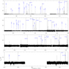 |
Fig. 1 Complete spectrum of V1057 Cyg obtained with the IRAM 30 m telescope. The selected lines are labeled with the name of the molecular species. The complete list of identified lines is provided in Table A.1, and zoom views of all lines are displayed in Fig. 2 and Figs. A.1–A.10 in Appendix A. The deep absorption features around 242–244 GHz and 258–259 GHz represent residual atmospheric absorption. |
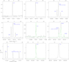 |
Fig. 2 Selection of lines detected with the IRAM 30 m telescope, labeled with the molecular species name in blue; the other lines are shown in Figs. A.1–A.9. LTE synthetic spectra are overlaid in green for selected species (see Sects. 3.4 and 3.5). In each panel, the bottom and top axes are labeled in frequency and velocity, respectively. |
3 Results and analysis
3.1 Line detection and identification
Figure 1 presents the complete spectrum obtained toward V1057 Cyg with the IRAM 30 m telescope. The frequencies of prominent lines are marked with vertical lines. The line identifications were based on spectroscopic data from the Cologne Database for Molecular Spectroscopy7 (CDMS, Müller et al. 2001, 2005) and the Jet Propulsion Laboratory catalog8 (JPL, Pickett et al. 1998). A line was considered detected when its peak intensity is ≥3σ, where σ is the rms noise level measured in the portion of the spectrum surrounding the candidate line. We only report lines of molecules with at least two detected transitions within the coverage of our line survey. In general, the detected lines are relatively narrow (<2.5 km s−1) and well isolated. Their identification is therefore straightforward compared to line-rich sources, such as hot cores or hot corinos (in high- mass or low-mass star-forming regions; e.g., Belloche et al. 2013; Bianchi et al. 2020; Busch et al. 2024). Figure 2 shows examples of the detected line profiles for several molecules observed with the 30 m telescope. These examples illustrate the identification of molecules with specific transitions (e.g., DCO+), hyperfine-structure components (e.g., CN), multiple transitions within a narrow frequency range (e.g., CH3OH), and broad wings indicating outflow activity (e.g., 13CO). The complete list of identified lines is given in Appendix A with upper energy levels, Einstein coefficients, and the parameters derived from Gaussian fits (discussed in Sect. 3.2), while each detected line is displayed in a narrow frequency window. In several cases, the data suggest potential detections of molecules, but these identifications remain uncertain because the signal-to-noise ratios are low (with candidate lines detected <3σ) or because they are based on a single weakly detected transition (below <3σ). These occurrences are not included in the final line identification and fit results in Table A.1 in Appendix A, but are instead marked with green labels in Figs. A.1–A.9 (e.g., some transitions of H2CO, H2CN, H5CN, and CH3OH in Fig. A.7. The list of identified lines from the APEX observations is given in Table A.2 in Appendix A, and the detected lines are displayed in Figs. A.10–A.13.
We detected emission of molecules ranging from simple neutral molecular species to COMs. The identified species are listed in Table 3, and the molecules appear from the simplest to the most complex. In total, 35 molecular species were detected (including isotopologs) in the spectrum of V1057 Cyg. We detected C-, N-, O-, and S -bearing molecules (e.g., CO, CN, CS, CCS, HCN, HNC, H2CO, and H2CS), deuterated species (e.g., DCN, and DNC), molecular ions (e.g., HCO+ and HCS+), carbon-chain molecules (e.g., C2H and HC3N), a cyclic molecule (e.g., c-C3H2), COMs (e.g., CH3OH), and in many cases, some of their isotopologs (see Table A.1).
The spectral energy distribution (SED) of V1057 Cyg implies a flared disk and envelope geometry (e.g., Kenyon & Hartmann 1991), while an envelope with an estimated size of 7000 au was confirmed from Spitzer/IRS observations (Green et al. 2006), and later, 50–670 µm far-infrared/submilllimeter wavelength imaging with Herschel indicated a reservoir of cold dust (Green et al. 2013). Based on 13CO observations using the Plateau de Bure Interferometer (with a beam of 2.7″× 2.2″), Fehér et al. (2017) reported a rotating envelope around V1057 Cyg with a radius of 5″ (3000 au). Thus, it is likely that our single-dish data, with a beam size larger than 9″, corresponding to ∼8100 au at the 897 pc distance to the target, trace emission from the disk and the envelope around the source. For instance, CO and its isotopologs likely trace the disk and outflow, while CS (2–1), HCN (1–0), and the hyperfine-structure components of CN (2–1) and C2H (1–0) could sample the cold gas closer to the midplane (seen in T Tauri stars, e.g., Dutrey et al. 2014). We also detected other dense gas tracers, such as CS, CCS, and HCO+, including their isotopologs 13CS, C33S, and C34S, and H13CO+ and N2H+ (e.g., Shirley 2015; Yamamoto 2017, and references therein).
For most molecular species, several transitions with different upper-level energies were detected, which allowed us a more detailed analysis, including simple radiative transfer modeling and the construction of population diagrams. This is presented in Sects. 3.4 and 3.5, respectively.
Overview of the molecules and isotopic species detected toward V1057 Cyg.
3.2 Line profiles, LSR velocities, and line widths
Based on single-dish observations, it can be challenging to distinguish emission from foreground or background clouds and from different physical structures within a source (e.g., disk and envelope) unless these components have different velocities. In this survey, we only detected molecules with similar velocities, suggesting that the observed line emission is associated with V1057 Cyg and its environment.
Most of the detected lines show narrow single-peaked profiles that can be fit by a single Gaussian. In the case of outflow tracers (e.g.,13 CO), the line profiles are also single peaked (except 12CO, see below), but show broader wings. This suggests outflow activity. For the spectrum at the source position, each line profile was fit with a single-Gaussian component using the built-in function in CLASS, and the results are presented in Tables A.1 and A.2. The Gaussian fitting method does not yield good results for the 12CO transitions because they show self-absorption, suggesting that these lines are optically thick (see examples for other FUors in Evans et al. 1994; Kóspál et al. 2017a; Kóspál 2011; Cruz-Sáenz de Miera et al. 2023). Therefore, these lines are only reported as detected in Tables A.1 and A.2, and no Gaussian fit results are presented. The LSR velocities obtained from the Gaussian fits range from 2.45 to 4.80 km s−1 for the 30 m and from 3.95 to 4.46 km s−1 for the APEX data.Compared to single-dish and interferometric observations from the last decade, we find that the previously reported velocities of, for example, 13CO (1–0) (4.6 and 4.05 km s−1, Kóspál 2011; Fehér et al. 2017), C18O (1–0) (4.10 km s−1, Kóspál 2011), and NH3 (1,1) (4.35 km s−1, Szabó et al. 2023a) are generally within ∼0.5 km s−1 of the vlsr values derived in this study. This further indicates that the molecular species detected in our survey are associated with V1057 Cyg and its environment. Notably, we find that the measured velocities of dense gas tracers such as CS, CCS, H13CO+, N2H+, and HC3N coincide within ∼0.3 km s−1 (within the uncertainties of the Gaussian fits) with the systemic velocity of V1057 Cyg derived from the most recent ammonia observations (4.35 ± 0.02 km s−1, Szabó et al. 2023a).
From the Gaussian fits, we find FWHM line widths between 0.67 and 3.43 km s−1 for the 30 m and from 0.71 to 1.78 km s−1 for the APEX data. In general, the FWHM line widths of lines that show wings, indicating outflow activity, are broader than those of the other species (e.g., 12CO and its isotopologs). The line widths of more than >50% of the fitted lines cluster around 1.3–1.5 km s−1 mainly for the transitions of CH3 OH, HC3N, and H2CO. Narrower widths are mainly found for CN and c- C3H2 lines, the former clustered around 1.1 km s−1 and the latter around 0.9–1 km s−1.
We note that the transition of methanol (CH3OH) at 84.5 GHz is a well-known Class I maser line (e.g., Batrla & Menten 1988; Breen et al. 2019, and references therein). However, the line emission detected toward V1057 Cyg does not show clear maser characteristics (e.g., strong, and narrow features in comparison to other transitions), which does not suggest maser activity. The well-known Class I CH3OH maser line at 95.1 GHz (Plambeck & Menten 1990; Chen et al. 2011; Yang et al. 2023) was not detected in our survey. We discuss this in Sect. 3.5.
Parameters of our best-fit LTE model and population diagram fit of methanol, formaldehyde, thioethenylidene, cyanoacetylene, thioformaldehyde, carbon monosulfide, and cyclopropenylidene.
3.3 Line mapping
Figures 3 and 4 present integrated-intensity maps for lines mapped in the otf mode with the IRAM 30 m and APEX 12 m telescopes, respectively. In most cases (except for 13CO 1–0 and 2–1; see Figs. 3i and 4b), the molecular line emission does not peak on V1057 Cyg itself. The HCN (1–0) HNC (1–0), HC3N (10–9), HCO+ (1–0), and N2H+ (1–0) maps show a primary concentration of emission offset from V1057 Cyg toward the north, while a secondary peak is distributed toward the southwest, connected with a ridge that traces a parsec-scale filamentary structure (Figs. 3c,d,f,g,h). The northern peak is offset by approximately 14.7″ (∼0.06 pc) to the north, while the southern peak is located approximately 1.8′ (∼0.46 pc) southwest of V1057 Cyg. The offset of the northern concentration relative to V1057 Cyg corresponds to only half a beam width in the 3 mm maps, but given the high signal-to-noise ratio of most maps, it is significant. It is probably not the result of an optical depth effect because 13CO (1–0) does peak toward the source. Moreover, the offset is larger than the pointing error. Furthermore, this peak is also visible in the dust-based H2 column density map (Szabó et al. 2023a). The larger-scale ridge structure is well traced by the 1–0 and 2–1 transitions of 13CO and C18O (see Figs. 3i,j and 4b,c). The ridge toward the southwest appears to be fainter than the northern peak seen in the maps of the 1–0 transitions of HCN, HCO+, and N2H+. Notably, the extent of the emission from some transitions (e.g., HC3N 10–9 and HNC 1–0) to the southwest seems comparable in size and intensity to that of the northern peak. The integrated-intensity maps of CCS (7– 6), H2CS (3–2), and HC3N (12–11) have lower signal-to-noise ratios, but appear to trace the same extensions toward the north and southwest.
The molecular outflow of V1057 Cyg was first reported by Evans et al. (1994) on the basis of the strong blueshifted wing emission detected in their 12CO 3–2 spectrum obtained with the Caltech Submillimeter Observatory 10.4 m telescope (CSO). These authors also mentioned the existence of maps toward this source as a private communication from S. McMuldroch, but we were unable to find any publication reporting them. The APEX spectrum has a similar line profile as the CSO spectrum, with a slightly more pronounced self-absorption, but our more sensitive spectrum reveals the redshifted wing for the first time. The APEX map of the 12CO 3–2 emission, presented in Fig. 5, reveals a bipolar outflow that appears to originate from V1057 Cyg. The outflow appears to be more collimated on the redshifted side, with discrete peaks south of the source position. Fig. 6 shows a 12CO (3–2) position-velocity (p-v) diagram taken along the cut shown in Fig. 5. The p-v diagram shows several peaks (labeled R1, R2, and B1; R for red and B for blue), which are more prominent in the redshifted emission. The highest- velocity extensions are revealed by the first contour close to R1, which may mark an episodic ejection event (Plunkett et al. 2015). Peak R1 appears close to the systemic velocity of the source, and peak R2 is located around 5 km s−1. The fainter blueshifted peak, B1, appears at a velocity around 1 km s−1. The p-v diagram also shows weak fingers (indicated by white arrows) revealed by the lowest contours of the 12CO emission. These results are further discussed in Sect. 4.2.
3.4 Radiative transfer modeling
The observed spectra were modeled using Weeds (a GILDAS/CLASS extension for the analysis of millimeter and submillimeter data, Maret et al. 2011) to create synthetic spectra with the assumption of local thermodynamic equilibrium (LTE). The spectroscopic information required for the synthetic spectra was taken from the CDMS database (Müller et al. 2005; Endres et al. 2016). Multiple transitions were detected from molecules such as methanol (CH3OH), formaldehyde (H2CO), cyclopropenylidene (c-C3H2), carbon monosulfide (CS), thioethenylidene (CCS), cyanoacetylene (HC3N), and thioformaldehyde (H2CS) (see Tables 4 and A.1. These species were chosen because several of their lines show significant emission (i.e., >3σ) and their profiles show no indication of outflow (i.e., extended wings, as seen in the lines from 12CO and its isotopologs). Only transitions detected with the IRAM 30 m telescope with a signal-to-noise ratio higher than 3σ were used for the following analysis. The radiative transfer model presented here, along with the population diagrams in Sect. 3.5, provides initial estimates of the temperatures and column densities of V1057 Cyg and its surrounding environment as observed in the single-dish data.
We applied a Weeds model to the chosen molecules to improve the line identification and to investigate whether the spectrum was well represented by an LTE model. The radiative transfer was computed by accounting for the line optical depth and the angular resolution of the observations. Weeds requires five input parameters for each molecule: the size of the emitting region (θs) in arcseconds, the column density (Ntot), the temperature (Trot), the line width (∆v in km s−1), and the velocity offset (voff, with respect to the systemic velocity of the source). For each molecule, the line width was set to the average value of the line widths determined from the Gaussian fits of its detected transitions. The column density and rotational temperature were set by eye and were subsequently adjusted until the best-fit was achieved. The population diagrams described in Sect. 3.5 were used to optimize the temperature and emission size and in turn the column density of the Weeds models to reach the best possible fits.
We explored a range of source sizes between 1.5″ (e.g., Calahan et al. 2024a) and 35″ (larger than the largest beam size) and found the best fits with a source size of 25″ for HC3N and 30′′ for the rest of the molecular species. These results are consistent with the integrated-intensity maps of the different species (see Fig. 3), and they are further discussed in Sect. 3.5. Calahan et al. (2024a) detected methanol emission toward V1057 Cyg using the NOEMA interferometer. This emission remained unresolved. The authors derived the column density and temperature of methanol with a similar LTE analysis, assuming a size of 1.5″ (Calahan priv. comm.). The same parameters in our Weeds model of the single-dish data resulted in methanol lines that were much weaker than those detected with the 30 m telescope. The 218.44 GHz methanol line is detected in interferometric and single-dish data. The peak intensity of this line is 53 mJy/beam in the NOEMA data (Calahan priv. comm.) and 440 mJy/beam in the IRAM 30 m telescope spectrum, which is ∼8.3 times higher. Since the CH3OH emission in the NOEMA data was unresolved (Calahan et al. 2024a), this difference implies that the single-dish observations trace extended emission that is not detected by the interferometer. With the single-dish telescope, we probably capture several components that are blended, including the disk and envelope and the surrounding cloud emission.
The best-fit column densities from our LTE modeling were used to derive abundances relative to H2. We derived values for the H2 column density by following the method of Szabó et al. (2023a, and references therein). We used archival Herschel data at 160, 250, and 350 µm to fit a spectral energy distribution (SED) to the data and derived H2 column densities at 25″ and 30″ resolution (corresponding to the sizes mentioned above) using the same method as used by Szabó et al. (2023a). However, unlike Szabó et al. (2023a), we did not use the 500 µm data because their angular resolution is relatively poor (37″). Based on the SED fit, we found H2 column densities of 1.14×1022 cm−2 and 1.21×1022 cm−2 at the angular resolution of 30″ and 25″, respectively (beam centered on the optical stellar position), with typical uncertainties of about 10%. The derived column densities and abundances are further discussed in Sect. 3.5 and are listed in Table 4. In a number of cases (especially for certain transitions of methanol), the LTE synthetic spectra do not match the observed spectra that well. Their excitation may deviate from LTE. Non-LTE modeling is beyond the scope of this work.
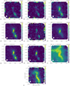 |
Fig. 3 Integrated-intensity maps of molecular lines obtained with the IRAM 30 m telescope. The red cross marks the position of V1057 Cyg, and the white circle shows the telescope beam size at the line frequency. The physical scale is presented near the beam size. The contour levels are nσint (multiples of the noise level in each map), and the corresponding values of n are given above each panel. |
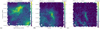 |
Fig. 4 Same as Fig. 3, but for the maps of (a) 12CO, (b) 13CO, and (c) C18O (2–1) obtained with APEX. |
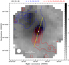 |
Fig. 5 Integrated-intensity map of 12CO (3–2) (grayscale image). The blue and red contours represent the blue- and redshifted wing emission integrated over the velocity ranges of [−6, 2] km s−1 and [5.5, 12] km s−1. The HPBW is shown in the bottom left corner in white. The position of V1057 Cyg is marked with a white cross. The yellow line shows the cut used for the position-velocity diagram in Fig. 6. The position angle (PA) of the cut is −17° (east from north). |
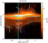 |
Fig. 6 Position-velocity (p-v) diagram along the yellow line shown in Fig. 5. The horizontal dashed cyan line corresponds to the systemic vlsr velocity of 4.35 km s−1 (Szabó et al. 2023a), and the vertical line corresponds to the source position. The contours start at 5σ and end at 35σ with 5σ steps in between. The peaks of the redshifted emission are labeled R1 and R2, and the peak of the blueshifted emission is labeled B1. The white arrows highlight the weak fingers that may trace episodic ejection events. |
3.5 Population diagrams and abundances
The transitions used for the population diagrams are well isolated in the spectrum of V1057 Cyg, and therefore, it was not necessary to discard any transitions owing to contamination by other species (a potential issue in line-rich sources; e.g., Belloche et al. 2009, 2016). The population diagrams were constructed using the integrated intensities of the observed profiles, and they are presented in Fig. 7. The fit results are given in Table 4. The population diagrams presented in this paper account for beam dilution using the sizes determined in Sect. 3.4, including the changing beam size through the frequency coverage. Additionally, the diagrams were also corrected for optical depth using the opacity correction factor  (see Goldsmith & Langer 1999) from the Weeds model.
In the case of methanol (Fig. 7a), we separated the A- and E- type transitions using two shades of green to test for a systematic difference, but we found none. The population diagram is also a good way to detect indications of maser activity of known maser species. The methanol emission in the 84.5 GHz transition does not deviate from the rest of the transitions in Fig. 7a, and it therefore does not indicate maser activity. However, we note that the best-fit model with Weeds underestimates the line strength. The other common maser transition at 95.1 GHz was not detected in this survey.
In all cases, a linear trend is present without significant departure from the linearity that could indicate the effect of optically thick emission or subthermal excitation (e.g., Velilla Prieto et al. 2017). The assumed emission size can affect the spread of data points in the population diagram due to the frequency-dependent beam size, while the opacities were found to be <<1 for all transitions and thus do not affect the shape of the diagrams. We checked the emission from CH3OH, from which multiple lower-frequency transitions (below 120 GHz, ∼3 mm window) are detected, and we found that assuming emission sizes smaller than 30″ increased the spread of the data points. This led to a larger gap between the low- and high-frequency transitions, which in turn compromised the fit to the data.
From the population diagram method, we find column densities ranging from 2.8×1013 cm−2 for CH3OH to 1.4×1012 cm−2 for H2CS, and rotational temperatures ranging from 8.1 K to 14.8 K. The Weeds models were optimized on the basis of the population diagram results. The two methods agree within the errors of the population diagram method for the column density and rotational temperature values.
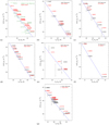 |
Fig. 7 Population diagrams of (a) CH3OH, (b) H2CO, (c) CCS, (d) HC3N, (e) H2CS, (f) CS, and (g) c-C3H2. The black points (green in the case of CH3OH) represent the observations, and the red points correspond to the Weeds synthetic spectra computed with the parameters given in Table 4. The blue line shows a fit to the observed data points. |
4 Discussion
4.1 Large- and small-scale structures in the environment of V1057 Cyg
In Sect. 3.3 we presented the integrated-intensity maps of several molecular species that in most cases trace lower-energy transitions (Figs. 3 and 4). We discuss the different structures traced in our single-dish observations in the environment of our target and compare our findings with those in the literature below.
The observed molecular emission traces a ridge structure that is dected in most of the integrated-intensity maps, with two peaks that are offset from V1057 Cyg: one peak toward the north at ∼14.7′′, and the other peak toward the southwest at ∼1.8′. The interferometric 13CO (1–0) data presented by Fehér et al. (2017) showed a structure north of V1057 Cyg that was referred to as clump B, with a similar offset as was detected in the singledish data. Their maps showed the close vicinity of V1057 Cyg and did not cover the southwestern extension. Extended 850 µm emission distributed over large scales was reported by Sandell & Weintraub (2001), who used the Submillimeter Common User Bolometer Array (SCUBA) on the James Clerk Maxwell Telescope. These authors found that V1057 Cyg was located on a narrow ridge that was traced by the dust continuum emission and extended north and southwest of the star. Our single-dish data extend farther to the southwest and provide more information. The ridge to the southwest detected in our molecular line data is visible in Herschel dust-based H2 column density maps (Szabó et al. 2023a). The dust map, along with our integrated- intensity maps, further suggests the large-scale morphology of a filamentary cloud, in which V1057 Cyg is located, as proposed by Sandell & Weintraub (2001).
Ridge structures or filaments, similar to what is seen around V1057 Cyg, are typically found in star-forming regions (e.g., André et al. 2010; Hacar et al. 2023, for a recent review). A famous example is the Taurus molecular cloud 1 (TMC-1), in which numerous cloud cores are located along a ridge structure (e.g., Hirahara et al. 1992; Langer et al. 1995). The size of the TMC-1 filaments is much larger (∼10 pc with cores around 0.1 pc in size, e.g., L1495 in TMC-1, Schmalzl et al. 2010) than the ridge we detected around V1057 Cyg (∼1–1.5 pc) within our field of view. Ridges with similar sizes as the ridge seen around V1057 Cyg were found in many low-mass starforming regions, and NGC 1333 is a prominent example (e.g., Hacar et al. 2017). We speculate that the condensation detected southwest of V1057 Cyg in high-density tracers (see Sect. 3.3) represents a secondary possibly protostellar dense core in the vicinity of V1057 Cyg. The spatial extent of the 850 µm data of Sandell & Weintraub (2001) did not reach far enough to the south to localise the peak, but the Herschel-derived H2 column density map shows a peak at the position of the southwestern peak that we detected in our single-dish molecular line data (see, e.g., Green et al. 2013; Szabó et al. 2023a, and Fig. C.1 in the latter).
Previously, the NH3 (1,1) transition toward V1057 Cyg was detected with a beam size of ∼37″ using the Effelsberg 100 m telescope (Szabó et al. 2023a). In light of our 30 m single-dish map of, for example, the N2H+ (1–0) emission, itis plausible that the NH3 spectrum is contaminated by the northern peak, which is located at ∼15″ offset of V1057 Cyg. High angular resolution observations of high-density tracers with interferometers might probe whether V1057 Cyg is an isolated protostar or a member of a cluster, similarly to the RNO 1B/1C FUor system (Quanz et al. 2007).
Properties of each lobe of the outflow of V1057 Cyg determined from the APEX 12CO 3–2 observations.
4.2 Temporal variations in the molecular outflow
We used single-dish and interferometric observations of 12CO (and its isotopologs) to identify molecular outflows associated with FUors and FUor-like objects (e.g., Evans et al. 1994; Kóspál 2011; Fehér et al. 2017; Kóspál et al. 2017a; Cruz-Sáenz de Miera et al. 2023, and references therein). As presented in Sect. 3.3, the molecular outflow of V1057 Cyg was first reported by Evans et al. (1994) only based on blueshifted wing emission in a single 12CO 3–2 spectrum of the source observed with the Caltech Submillimeter Observatory 10.4-meter telescope (CSO). Our new12 CO (3–2) APEX map reveals a clear bipolar outflow morphology (Fig. 5), and the redshifted component is reported here for the first time. We note that the CSO spectrum of Evans et al. (1994), which peaks at 8.7 km s−1, is shifted by about 4.5 km s−1 compared to the APEX spectrum. This discrepancy is puzzling. Although the Gaussian fit is unreliable for the 12CO data, it would still be closer to our 13CO and C18O (1–0) vlsr of 3.86 km s−1 and 4.09 km s−1, and also to those derived from interferometric data by Fehér et al. (2017) for 13CO and C18O (1–0) with values of 4.05 km s−1 and 4.10 km s−1, respectively. We suspect that the frequency axis of the spectrum published in Evans et al. (1994) was not properly calibrated.
Figure 5 reveals the outflow originating from V1057 Cyg. The redshifted lobe points south-southeast, and the blueshifted lobe points north-northwest. We measured the length of the lobes, Rlobe, and maximum velocities, v′max, to estimate the dynamical time, td, of the outflow with the formula  with i the inclination of the outflow axis to the line of sight (summarized in Table 5, Beuther et al. 2002). The outflow map shows a bipolar morphology without overlap between the red- and blueshifted emissions. This implies an intermediate inclination angle. Therefore, we estimated td assuming a range of inclinations between 10° and 80° and obtained values ranging from 5×10³ yr to 234×103 yr. Previous studies that analyzed the disk of V1057 Cyg derived an inclination of 62° (Liu et al. 2018; Szabó et al. 2021). In the following, we adopt the dynamical times estimated with 62°, which is 15 000 years for the blue lobe and 22 000 years for the red lobe of the outflow of V1057 Cyg. A survey of 20 FUors, also using the APEX 12 m telescope (Cruz-Sáenz de Miera et al. 2023), found dynamical times on the order of thousands of years, from 3×10³ yr to 130×103 yr. This suggests that the detected outflows are most likely not related to the current outbursts in the sample. V1057 Cyg has been in outburst for about 50 years (Herbig 1977; Herbig et al. 2003; Clarke et al. 2005; Szabó et al. 2021), and therefore, the outflow cannot result from the ongoing outburst alone. High-velocity gas may have been ejected in the recent outburst, but this gas would be confined to small scales and remain unresolved in singledish observations (see also the results of Cruz-Sáenz de Miera et al. 2023).
Signs of potential previous ejection activity in V1057 Cyg have not yet been explored. One way to search for historical mass-ejection events is to inspect the kinematics of the outflow in a position-velocity (p-v) diagram, which can be used as a fossil record (e.g., Arce & Goodman 2001; Zhou et al. 2024). The p-v diagram displayed in Fig. 5 shows discrete peaks and indicates structures similar to the turbulent jet + jet bow-shock model. This can be interpreted as episodic accre- tion/ejection events (see, e.g., Plunkett et al. 2015). In this model, the episodic variation in the jet velocity produces an internal bow shock driving an internal shell in addition to the terminal shock. The 12CO emission traces cool (i.e., lower than 100 K) swept-up material, providing a record of the timing history of mass-loss event(s). Our p-v diagram shows blue- and redshifted peaks (R1, R2, and B1 in Fig. 6), with velocity offsets from the systemic velocity of V1057 Cyg. Moreover, the p-v diagram shows weak fingers that are revealed by the lowest contour in the blue- and redshifted emission (indicated by white arrows in Fig. 6). This is reminiscent of the results of Plunkett et al. (2015), who reported a saw-like pattern along the extent of the 12CO emission of the Class 0 source CARMA-7. Plunkett et al. (2015) proposed that the peaks might indicate shocks and that the fingers (in their case, the saw-like structure) might be evidence for a period in which the faster ejecta overtakes the slower ejecta. Furthermore, previous ejections could entrain the outflow material and might therefore appear to be clumpy (see peaks R1, R2, and B1 in Fig. 6). This might create distinct shocks when a newer ejecta overtakes the previous older ejecta (Plunkett et al. 2015). The clumpy structure of the 12CO emission of V1057 Cyg might indicate episodic ejection mechanisms and not a smooth, continuous/homogeneous outflow. The prominent peaks and weak fingers complemented with the estimated dynamical times further suggest previous outburst activity of V1057 Cyg.
4.3 Brief comparison to other FUors
Millimeter-wavelength observations can provide information on the small and large scales in the environments of YSOs. The majority of previous studies of FUors, whether singledish or interferometric observations, mainly focused on 12CO and its rarer isotopologs of 13CO and C18O to probe the molecular outflows (e.g., Evans et al. 1994; Fehér et al. 2017; Ruíz-Rodríguez et al. 2017b; Ruíz-Rodríguez et al. 2017a; Hales et al. 2020; Wendeborn et al. 2020; Cruz-Sáenz de Miera et al. 2023; Nogueira et al. 2023, and references therein). However, other molecular species have increasing been employed over the past decade using single-dish and interferometric facilities. Despite being a famous member within its class and a classical FUor, V1057 Cyg has not yet been systematically searched for molecular emission in the millimeter domain. Similar to the detailed optical and near-infrared studies (see, e.g., Herbig et al. 2003; Szabó et al. 2021, 2022), this might be valuable for the classification of new FUors. Prior to this work, molecular line observations toward our target mainly focused on 12CO (and its isotopic species), which has been observed since the 1970s, following the outburst. 12CO and 13CO 1–0 line emission was first reported by Bechis & Lo (1975), followed by the detection of other transitions of 12CO and its isotopic species throughout the decades, conducted with singledish telescopes and interferometers (see Sect. 3.2). The detection of the simple molecule CN (3–2) was also reported toward V1057 Cyg with a peak vlsr comparable to the 12CO observations (Stäuber et al. 2007). The recent NOEMA observations by Calahan et al. (2024a) showed that V1057 Cyg stands out among a small sample of surveyed eruptive YSOs, with detections of several COMs (e.g., CH3OH, CH3CN, and CH3OCHO), sulfurbearing molecules (e.g., SO and SO2), and others. In the following, we give a brief overview of the most relevant molecular line studies targeting FUors and briefly compare their results to ours. These include single-dish and interferometric observations. For the relevant comparison, we mention RNO 1B/1C, L1551 IRS5, and V883 Ori. It is important to note that beam dilution is an important factor when comparing single-dish and interferometric studies because it limits the capability of single-dish telescopes to detect compact emission.
For the overview, we constructed Table 6, which lists a selection of species ranging from simple molecules to COMs. The table indicates the sources for which a detection has been reported for each molecule. The FUor binary RNO 1B/1C is one of the earliest documented examples of molecular emission associated with FUors (apart from CO, Evans et al. 1994), which include detection of SiO (5–4), H2CO (3–2), CH3OH (4– 3), C18O (2–1), CS (7–6 and 2–1), and HCO+ (4–3) emission (McMuldroch et al. 1995). In this case, the CO emission was found to trace the bipolar outflow and CS (2–1) to probe the dense cloud core around the binary. In all cases, the authors find relatively cold (below 35 K) emission tracing the environment of RNO 1B/1C, which is similar to the cold molecular emission detected toward V1057 Cyg. The rotational temperatures that we derived toward V1057 Cyg are lower than those toward RNO 1B/1C, however. The column densities are lower by about an order of magnitude for V1057 Cyg than in RNO 1B/1C. Similarly to RNO 1B/1C, we also detected further indication of dense material (together with the previous NH3 observations and compact morphology of dust emission, Szabó et al. 2023a) from a number of transitions of CS, CCS, HCO+ (and their isotopologs), or N2H+ (see also, McMuldroch et al. 1995; Shirley 2015; Yamamoto 2017, and references therein), traced on single-dish scales.
The most prominent example in the literature for molecular line emission probably is the FUor-like Class I protostar L1551 IRS5 (e.g., Adams et al. 1987; Looney et al. 1997; Connelley & Reipurth 2018), which is located in Taurus at a distance of ∼140 pc (Zucker et al. 2019), with a luminosity of L = 28 L⊙ (Butner et al. 1991). This source might be one of the most line-rich sources associated with the class, and it includes the detection of molecular species ranging from simple to complex molecules (see Table 6, and also e.g., Fridlund et al. 2002; White et al. 2006; Mercimek et al. 2022, and references therein). The most notable result toward this source is the interferometric detection of a hot corino (a region around a low-mass protostar bright in emission of COMs, e.g., Yamamoto 2017) traced by CH3OH (and its isotopologs), CH2DOH, HCOOCH3, and CH3CH2OH (Bianchi et al. 2020). The most recent study of this source reported a survey covering the 3 mm and 2 mm windows using the 30 m telescope. This revealed a total of 75 species (including isotopologs, Marchand et al. 2024). V1057 Cyg is not as line rich as L1551 IRS5, and a lower number of species are detected, and in particular, only 3 COMs (CH3OH, CH3CCH, and CH3CN) out of the 15 reported by Marchand et al. (2024). The majority of species detected in the recent survey of L1551 IRS5 trace the cold envelope with temperatures ≤10 K, but the authors reported molecules with ≥5 atoms and a few S-bearing species (C3S, SO, SO2) to trace warmer ≥30 K regions. In V1057 Cyg, we do not detect molecular emission above 10K, implying that we only trace cold molecular emission toward this source. The column densities derived by the authors for L1551 IRS5 are within the same order of magnitude as the column densities we derived for V1057 Cyg, with the exception of c-C3H2, whose column density is lower by an order of magnitude (Marchand et al. 2024). However, we note that the emission detected by our single-dish observations extends over 25–30″, that is, ∼0.1 pc at the distance of ∼900 pc, and it likely traces the disk, the envelope, and the surrounding cloud, while the observations of L1551 IRS5 and V883 Ori traced smaller scales (see below).
Finally, we give a brief comparison to V883 Ori, a FUor that is in transit from Class I to Class II phase, located at a distance of d = 338 pc, with a bolometric luminosity of L = ∼220 L⊙ (e.g., Furlan et al. 2016; Connelley & Reipurth 2018; Lee et al. 2019). This source was the focus of a number of interferometric observations that in particular revealed a snowline shift that was attributed to the outburst, a complex physical structure of its environment traced by high-density (e.g., HCN, HCO+, DCN) and shock tracers (e.g., CH3OH, SiO, SO), a ring-like structure traced by HCO+ emission, and a rich chemistry traced by COMs (see Table 6 and also e.g., Ruíz-Rodríguez et al. 2017a, 2022; Lee et al. 2019; Yamato et al. 2024; Lee et al. 2024). The most recent study of Lee et al. (2024) focused on the detection of simple molecular species and a short list of COMs using ALMA Band 6 data. This frequency regime is partly covered by our singledish observations. We found many molecular species detected in V1057 Cyg and V883 Ori (see Table 6). The interferometic data trace different physical components of the environment of V883 Ori: HDCO and HNCO mainly trace the water-sublimation front, HCN emission traces the inner and outer disk, revealing an arm-like structure, and HNC and DNC trace a ring structure at the boundary of the outer disk (Lee et al. 2024). With the single-dish data of V1057 Cyg, we are only able to trace the large-scale emission (the ridge with the southern peak and northern concentration, and the outflow; see also Sects. 3.3, 4.1, and 4.2). Between these two sources, we find that V883 Ori harbors more COMs, similarly to L1551 IRS5. However, for the more evolved nature of V1057 Cyg, it still demonstrates a line-rich environment. This motivates follow-up interferometric observations. Furthermore, we did not detect water lines in this survey (despite transitions covered by the setup) compared to V883 Ori, but we note that HDO 3(1,2)–2(2,1) emission has recently been confirmed by sensitive interferometric NOEMA observations toward V1057 Cyg (Calahan et al. 2024a).
4.4 Chemical signatures of outbursts and outlook
Episodic outbursts may strongly influence the disks around protostars by introducing changes to the thermal structure and inducing chemical changes (e.g., Fischer et al. 2023). This may be used to identify previous outburst events.
Rab et al. (2017) extended the radiation thermochemical disk code PRODIMO (PROtoplanetary DIsk MOdel, Woitke et al. 2009, 2016) to treat envelope structures by feeding a representative Class I model. They used simulated spatially resolved ALMA C18O 2–1 observations and found this particular transition to be a good tool for probing post-outburst sources. In the model, the spatially resolved 2–1 transition emission exhibits distinct signatures, such as a gap due to the freeze-out of the molecules (see Fig. 4 of Rab et al. 2017). In our line survey, we detected and mapped the C18O 2–1 transition with APEX, and the emission is resolved in the north-south direction, tracing the ridge. Our observations did not resolve the disk around V1057 Cyg, however (see Fig. 4 and Table A.2). Interferometric observations of the C18O 1–0 transition by Fehér et al. (2017) found a rotating envelope with a radius of 5″, or 3000 au at d = 600 pc (common distance used before Gaia, Bailer-Jones et al. 2018a,b), corresponding to ∼4500 au at ∼900 pc. With the singledish observations of this transition with a beam size of 22.4″, we do not resolve the envelope either, however. The model of Rab et al. (2017) accounted for the disk and envelope emission, and the outburst-induced changes are seen in the radial distribution of the 12CO emission on scales of a few 1000 au. This is much larger than typical disk scales. Our single-dish observations have an angular resolution that corresponds to about ∼18 000 au, and they therefore cannot resolve the 12CO structures predicted by the model, which are at scales of a few 1000 au.
The other notable model was reported by Molyarova et al. (2018), who used the ANDES physical-chemical code (Akimkin et al. 2013) to follow the impact of a FUor outburst on the chemical evolution and to identify molecular tracers on different timescales. Two main groups were specified: species with abundances sensitive to the ongoing outburst that quickly returned (i.e., a few years after the peak outburst) to the quiescent (pre-outburst) values; and those that took longer to return to preoutburst or even remained overabundant for decades (>20 yr). The most notable prediction was formaldehyde (H2CO), whose abundance can grow by up to 4–6 magnitudes, and which takes 30–120 years to deplete back onto dust grains. This makes it a good candidate tracer in theory for identifying post-outburst sources. The authors modeled the brightest H2CO transition observed in disks, the 303–202 transition at 218.222 GHz, with input parameters based on the FUor outburst of V346 Nor, which in 2010 seemed to abruptly cease its outburst (and was thought to be the first FUor to do so, see Kraus et al. 2016). However, the study of Kóspál et al. (2020) showed evidence that the source gradually brightened again to almost the same brightness level as before the abrupt fading event, and they concluded that the fading was likely due to different mechanisms, including an increase of the line-of-sight extinction, and the appearance of warm material that may have refuelled the outburst. We detected the H2CO (303–202) transition toward V1057 Cyg in the 30 m data, but it is fainter than other transitions of H2CO detected in the survey. We found that the abundances of H2CO and CH3OH (see Table 4) were lower by several orders of magnitude than the abundances predicted by the medium and grown dust models by Molyarova et al. (2018). However, our abundances correspond to material at the scale of ∼30″, while the model abundances are predicted at the much smaller scale of the disk. In contrast, the HC3N abundance is closer to the model predictions, although its abundance is lower than those of H2CO and CH3OH. We note that our HC3N map shows extended emission, without a peak centered on V1057 Cyg. This suggests that the HC3N line emission detected toward the target is not dominated by compact unresolved emission. We lack maps of H2CO or CH3OH emission to confirm whether the emission peaks on the target. The CS abundance derived for V1057 Cyg is higher than the model predictions. The NH3 abundance derived in an earlier study (Szabó et al. 2023a) is lower by about one order of magnitude than the abundance predicted by the model of Molyarova et al. (2018).
Considering that V1057 Cyg has been in outburst for over 50 years, it is plausible that during the peak of the outburst, the abundance values were elevated due to the heat from the central source. The detection of multiple transitions of many molecular species and the lower abundances compared to the model predictions show that many species are still present and are not yet frozen-out to dust surfaces. On the other hand, the single-dish data clearly trace large-scale structures (i.e., the ridge), and it is uncertain which fraction of the measured flux is related to a more compact disk around the source and which part is related to the extended ridge.
The available chemical models, together with line surveys such as the one presented here, motivate observational and theoretical follow-up studies. In the case of V1057 Cyg, high angular resolution observations might resolve the smaller-scale structures (i.e., on scales of the disk and envelope system) and their connection to the larger scale emission traced by the ridge north and south of the source position. Future spatially resolved observations can reveal similar structures predicted in the models due to the inside-out freeze-out (Rab et al. 2017), snowline shifts (either water or other molecules) attributed to the outburst, or help us to distinguish the species that trace the different layers in the system, similarly to what has been found in V883 Ori (e.g., Tobin et al. 2023; Yamato et al. 2024). This may allow us to probe the impact of the outburst on the physical and chemical structure of the disk and the close environment of V1057 Cyg (e.g., Molyarova et al. 2018; Lee et al. 2024; Andreu et al. 2023). Further detection of indicators of the water snowline (e.g., Molyarova et al. 2018) and information on the D/H ratio in more evolved sources such as V1057 Cyg may add more information on Class II sources that are currently absent from the statistics (see Fig. 3 of Andreu et al. 2023, and references therein). Although our single-dish data are unable to resolve the small scales, the line survey shows a richer line emission than might have been expected for a relatively more evolved classical FUor like V1057 Cyg, and this motivates higher angular resolution studies to determine whether emission from molecules such as H2CO and CH3OH comes from the large-scale ridge or a compact structure around the source. Furthermore, high angular resolution observations of 12CO might reveal previous episodic ejection events in greater detail.
5 Conclusions
We presented the first wide-band line survey in the millimeter wavelength regime of V1057 Cyg and its surrounding environment. This Class II source has been in outburst for about 50 years and has not yet shown signs of returning to quiescence (Szabó et al. 2021). The line survey has an almost continuous frequency coverage from ∼72 GHz to ∼263 GHz (with a spatial resolution between ∼36″ and ∼10″) with the IRAM 30 m telescope. Additionally, specific frequency ranges around 219, 227, 291, and 344 GHz (with a spatial resolution between ∼30″ and ∼19″) were observed with the APEX 12 m telescope. The line identification and analysis carried out on the data led to the conclusions listed below:
We identified (mostly) simple C-, N-, O-, and S -bearing molecules (e.g., CN, CS, and HCN), deuterated species (e.g., DCN), molecular ions (e.g., HCO+), more simple C- chain molecules (e.g., C2H and HC3N), and complex organic molecules. V1057 Cyg displays lines from 35 molecular species (including isotopologs). The different spatial distribution of emission in the integrated line intensity maps indicates that the various lines sample different regions in the environment of the source. Most of the lines detected in this survey were detected in disks around T Tauri stars (e.g., Dutrey et al. 2014), the closest in evolution to V1057 Cyg, and in other well-studied FUors (e.g., Marchand et al. 2024; Lee et al. 2024).
Most of the lines show narrow single-peaked line profiles that are well described by single-Gaussian fits, with the exception of outflow tracers, which show broader line wings that indicate outflow activity. The LSR velocities in all cases indicate that the line emission is associated with the circumstellar environment of V1057 Cyg.
Population diagrams of molecules detected in several transitions (CH3OH, H2CO, CCS, HC3N, H2CS, CS, and c- C3H2) were constructed. They indicate rotational temperatures (Trot) ranging from 8.1 K to 14.8 K. We derived the column densities (Ntot) of these molecules under the assumption of LTE, with values ranging from 1.4×1012 cm−2 to 2.8×1013 cm−2. The derived column densities are lower by about one order of magnitude than those derived for younger line-rich FUors, but our single-dish survey probes larger scales.
The emission of several molecular species was mapped with the IRAM 30 m or the APEX 12 m telescopes. The integrated-intensity maps trace a parsec-scale ridge that runs southwest to north, going through the position of V1057 Cyg. This ridge coincides with the ridge traced earlier in dust continuum emission (Sandell & Weintraub 2001; Green et al. 2013; Szabó et al. 2023a), but our molecular line maps cover a larger area toward the southwest. Two clumps of molecular emission that are clearly visible in the integrated-intensity maps of HCN, HNC, N2H+ 1–0, and HC3N 10–9, are detected along the ridge north and southwest of V1057 Cyg. They are offset by ∼15″ (∼0.06 pc), and ∼108″ (∼0.46 pc) from the source position. Our results might indicate that V1057 Cyg is forming as part of a small cluster, similarly to several other FUors (e.g., White et al. 2006; Quanz et al. 2007), and they motivate future interferometric observations to reveal the protostellar content of the filamentary structures.
Our new 12CO 3–2 map reveals a bipolar outflow centered on V1057 Cyg. We estimated a dynamical time for the outflow of several ten thousand years (15 000 years for the blue and 22 000 years for the red lobe of the outflow), implying that the detected outflow does not result from the current outburst activity alone. The position-velocity diagram showed discrete peaks and indicated structures that represent episodic ejection events. This further indicates outburst activity in the past evolution of V1057 Cyg.
Although it is located at a distance of almost 900 pc and is a more evolved (i.e., Class II) object, V1057 Cyg exhibits a line-rich environment in our single-dish observations. While the molecular emission in the environment of V1057 Cyg does not reveal clear evidence of the imprint of an outburst on the chemistry of the object on the scales traced by our single-dish data, the linerich spectra motivate interferometric observations to spatially resolve the emission. Our results also motivate similar studies of a larger sample of FUors to study the range of astrochemical properties associated with this class of outbursting protostars, and to improve the current statistics regarding the outburst effects on the chemical composition of their close environments. These are ultimately the future birthplace of planets.
Data availability
The data underlying this article and Appendix A (with the full list and figures of the line detections) are available on Zenodo, at https://zenodo.org/records/14745697 and https://zenodo.org/records/14754174, respectively.
Acknowledgements
We thank the anonymous referee for valuable feedback which has improved the quality of our manuscript. Zs. M. Szabó acknowledges funding from a St. Leonards scholarship from the University of St. Andrews and C. J. C. acknowledges support from the STFC (grant ST/Y002229/1). For the purpose of open access, the author has applied a Creative Commons Attribution (CC BY) licence to any Author Accepted Manuscript version arising. Y. G. is supported by the Strategic Priority Research Program of the Chinese Academy of Sciences, Grant No. XDB0800301. This work is based on observations carried out under project number 060-21 (PI: Karl M. Menten) with the IRAM 30m telescope. IRAM is supported by INSU/CNRS (France), MPG (Germany) and IGN (Spain). This publication is based on data acquired with the Atacama Pathfinder Experiment (APEX) under programme ID M9530C_107, M9515A_108, and M9523C_109. APEX has been a collaboration between the Max-Planck-Institut fur Radioastronomie, the European Southern Observatory, and the Onsala Space Observatory. This work was also supported by the NKFIH excellence grant TKP2021-NKTA-64.
References
- Adams, F. C., Lada, C. J., & Shu, F. H. 1987, ApJ, 312, 788 [NASA ADS] [CrossRef] [Google Scholar]
- Akimkin, V., Zhukovska, S., Wiebe, D., et al. 2013, ApJ, 766, 8 [NASA ADS] [CrossRef] [Google Scholar]
- André, P., Men’shchikov, A., Bontemps, S., et al. 2010, A&A, 518, L102 [CrossRef] [EDP Sciences] [Google Scholar]
- Andreu, A., Coutens, A., Cruz-Sáenz de Miera, F., et al. 2023, A&A, 677, L17 [NASA ADS] [CrossRef] [EDP Sciences] [Google Scholar]
- Arce, H. G., & Goodman, A. A. 2001, ApJ, 551, L171 [NASA ADS] [CrossRef] [Google Scholar]
- Audard, M., Ábrahám, P., Dunham, M. M., et al. 2014, in Protostars and Planets VI, eds. H. Beuther, R. S. Klessen, C. P. Dullemond, & T. Henning, 387 [Google Scholar]
- Bailer-Jones, C. A. L., Rybizki, J., Fouesneau, M., Mantelet, G., & Andrae, R. 2018a, AJ, 156, 58 [Google Scholar]
- Bailer-Jones, C. A. L., Rybizki, J., Fouesneau, M., Mantelet, G., & Andrae, R. 2018b, VizieR Online Data Catalog, I/347 [Google Scholar]
- Batrla, W., & Menten, K. M. 1988, ApJ, 329, L117 [NASA ADS] [CrossRef] [Google Scholar]
- Bechis, K. P., & Lo, K. Y. 1975, ApJ, 201, 118 [NASA ADS] [CrossRef] [Google Scholar]
- Belloche, A., Garrod, R. T., Müller, H. S. P., et al. 2009, A&A, 499, 215 [NASA ADS] [CrossRef] [EDP Sciences] [Google Scholar]
- Belloche, A., Müller, H. S. P., Menten, K. M., Schilke, P., & Comito, C. 2013, A&A, 559, A47 [NASA ADS] [CrossRef] [EDP Sciences] [Google Scholar]
- Belloche, A., Müller, H. S. P., Garrod, R. T., & Menten, K. M. 2016, A&A, 587, A91 [NASA ADS] [CrossRef] [EDP Sciences] [Google Scholar]
- Beuther, H., Schilke, P., Sridharan, T. K., et al. 2002, A&A, 383, 892 [NASA ADS] [CrossRef] [EDP Sciences] [Google Scholar]
- Bianchi, E., Chandler, C. J., Ceccarelli, C., et al. 2020, MNRAS, 498, L87 [NASA ADS] [CrossRef] [Google Scholar]
- Breen, S. L., Contreras, Y., Dawson, J. R., et al. 2019, MNRAS, 484, 5072 [NASA ADS] [CrossRef] [Google Scholar]
- Busch, L. A., Belloche, A., Garrod, R. T., Müller, H. S. P., & Menten, K. M. 2024, A&A, 681, A104 [NASA ADS] [CrossRef] [EDP Sciences] [Google Scholar]
- Butner, H. M., Evans, Neal J., I., Lester, D. F., Levreault, R. M., & Strom, S. E. 1991, ApJ, 376, 636 [NASA ADS] [CrossRef] [Google Scholar]
- Calahan, J. K., Bergin, E. A., van’t Hoff, M., et al. 2024a, ApJ, 975, 170 [NASA ADS] [CrossRef] [Google Scholar]
- Calahan, J. K., Bergin, E. A., van’t Hoff, M., et al. 2024b, ApJ, 967, 158 [NASA ADS] [CrossRef] [Google Scholar]
- Carter, M., Lazareff, B., Maier, D., et al. 2012, A&A, 538, A89 [NASA ADS] [CrossRef] [EDP Sciences] [Google Scholar]
- Ceccarelli, C., Caselli, P., Fontani, F., et al. 2017, ApJ, 850, 176 [NASA ADS] [CrossRef] [Google Scholar]
- Ceccarelli, C., Codella, C., Balucani, N., et al. 2022, arXiv e-prints [arXiv:2206.13270] [Google Scholar]
- Chen, X., Ellingsen, S. P., Shen, Z.-Q., Titmarsh, A., & Gan, C.-G. 2011, ApJS, 196, 9 [NASA ADS] [CrossRef] [Google Scholar]
- Cieza, L. A., Casassus, S., Tobin, J., et al. 2016, Nature, 535, 258 [Google Scholar]
- Clarke, C. J., Lodato, G., Melnikov, S. Y., & Ibrahimov, M. A. 2005, MNRAS, 361, 942 [NASA ADS] [CrossRef] [Google Scholar]
- Connelley, M. S., & Reipurth, B. 2018, ApJ, 861, 145 [NASA ADS] [CrossRef] [Google Scholar]
- Cruz-Sáenz de Miera, F., Kóspál, Á., Ábrahám, P., et al. 2023, ApJ, 945, 80 [CrossRef] [Google Scholar]
- Dutrey, A., Semenov, D., Chapillon, E., et al. 2014, in Protostars and Planets VI, eds. H. Beuther, R. S. Klessen, C. P. Dullemond, & T. Henning, 317 [Google Scholar]
- Endres, C. P., Schlemmer, S., Schilke, P., Stutzki, J., & Müller, H. S. P. 2016, J. Mol. Spectrosc., 327, 95 [NASA ADS] [CrossRef] [Google Scholar]
- Evans, I., Neal J., Balkum, S., Levreault, R. M., Hartmann, L., & Kenyon, S. 1994, ApJ, 424, 793 [NASA ADS] [CrossRef] [Google Scholar]
- Fehér, O., Kóspál, Á., Ábrahám, P., Hogerheijde, M. R., & Brinch, C. 2017, A&A, 607, A39 [CrossRef] [EDP Sciences] [Google Scholar]
- Fischer, W. J., Hillenbrand, L. A., Herczeg, G. J., et al. 2023, in Astronomical Society of the Pacific Conference Series, 534, eds. S. Inutsuka, Y. Aikawa, T. Muto, K. Tomida, & M. Tamura, 355 [NASA ADS] [Google Scholar]
- Fridlund, C. V. M., Bergman, P., White, G. J., Pilbratt, G. L., & Tauber, J. A. 2002, A&A, 382, 573 [NASA ADS] [CrossRef] [EDP Sciences] [Google Scholar]
- Furlan, E., Fischer, W. J., Ali, B., et al. 2016, ApJS, 224, 5 [Google Scholar]
- Goldsmith, P. F., & Langer, W. D. 1999, ApJ, 517, 209 [Google Scholar]
- Green, J. D., Hartmann, L., Calvet, N., et al. 2006, ApJ, 648, 1099 [NASA ADS] [CrossRef] [Google Scholar]
- Green, J. D., Evans, Neal J., I., Kóspál, Á., et al. 2013, ApJ, 772, 117 [CrossRef] [Google Scholar]
- Güsten, R., Nyman, L. Å., Schilke, P., et al. 2006, A&A, 454, L13 [NASA ADS] [CrossRef] [EDP Sciences] [Google Scholar]
- Hacar, A., Tafalla, M., & Alves, J. 2017, A&A, 606, A123 [NASA ADS] [CrossRef] [EDP Sciences] [Google Scholar]
- Hacar, A., Clark, S. E., Heitsch, F., et al. 2023, in Astronomical Society of the Pacific Conference Series, 534, Protostars and Planets VII, eds. S. Inutsuka, Y. Aikawa, T. Muto, K. Tomida, & M. Tamura, 153 [NASA ADS] [Google Scholar]
- Hales, A. S., Pérez, S., Gonzalez-Ruilova, C., et al. 2020, ApJ, 900, 7 [NASA ADS] [CrossRef] [Google Scholar]
- Hartmann, L., & Kenyon, S. J. 1996, ARA&A, 34, 207 [NASA ADS] [CrossRef] [Google Scholar]
- Herbig, G. H. 1966, Vistas Astron., 8, 109 [Google Scholar]
- Herbig, G. H. 1977, ApJ, 217, 693 [NASA ADS] [CrossRef] [Google Scholar]
- Herbig, G. H. 2009, AJ, 138, 448 [NASA ADS] [CrossRef] [Google Scholar]
- Herbig, G. H., Petrov, P. P., & Duemmler, R. 2003, ApJ, 595, 384 [Google Scholar]
- Herbst, E., & van Dishoeck, E. F. 2009, ARA&A, 47, 427 [NASA ADS] [CrossRef] [Google Scholar]
- Hillenbrand, L. A., Contreras Peña, C., Morrell, S., et al. 2018, ApJ, 869, 146 [NASA ADS] [CrossRef] [Google Scholar]
- Hirahara, Y., Suzuki, H., Yamamoto, S., et al. 1992, ApJ, 394, 539 [NASA ADS] [CrossRef] [Google Scholar]
- Hogerheijde, M. R., van Dishoeck, E. F., Salverda, J. M., & Blake, G. A. 1999, ApJ, 513, 350 [NASA ADS] [CrossRef] [Google Scholar]
- Jørgensen, J. K., Belloche, A., & Garrod, R. T. 2020, ARA&A, 58, 727 [Google Scholar]
- Kenyon, S. J., & Hartmann, L. W. 1991, ApJ, 383, 664 [NASA ADS] [CrossRef] [Google Scholar]
- Klein, B., Philipp, S. D., Krämer, I., et al. 2006, A&A, 454, L29 [NASA ADS] [CrossRef] [EDP Sciences] [Google Scholar]
- Kóspál, Á. 2011, A&A, 535, A125 [NASA ADS] [CrossRef] [EDP Sciences] [Google Scholar]
- Kóspál, Á., Ábrahám, P., Acosta-Pulido, J. A., et al. 2016, A&A, 596, A52 [NASA ADS] [CrossRef] [EDP Sciences] [Google Scholar]
- Kóspál, Á., Ábrahám, P., Csengeri, T., et al. 2017a, ApJ, 836, 226 [CrossRef] [Google Scholar]
- Kóspál, Á., Ábrahám, P., Westhues, C., & Haas, M. 2017b, A&A, 597, L10 [CrossRef] [EDP Sciences] [Google Scholar]
- Kóspál, Á., Szabó, Z. M., Ábrahám, P., et al. 2020, AJ, 889, 148 [Google Scholar]
- Kraus, S., Caratti o Garatti, A., Garcia-Lopez, R., et al. 2016, MNRAS, 462, L61 [NASA ADS] [CrossRef] [Google Scholar]
- Langer, W. D., Velusamy, T., Kuiper, T. B. H., et al. 1995, ApJ, 453, 293 [NASA ADS] [CrossRef] [Google Scholar]
- Lee, J.-E., Lee, S., Baek, G., et al. 2019, Nat. Astron., 3, 314 [Google Scholar]
- Lee, J.-E., Kim, C.-H., Lee, S., et al. 2024, ApJ, 966, 119 [NASA ADS] [CrossRef] [Google Scholar]
- Leemker, M., van’t Hoff, M. L. R., Trapman, L., et al. 2021, A&A, 646, A3 [EDP Sciences] [Google Scholar]
- Levreault, R. M. 1988, ApJS, 67, 283 [Google Scholar]
- Liu, H. B., Dunham, M. M., Pascucci, I., et al. 2018, A&A, 612, A54 [NASA ADS] [CrossRef] [EDP Sciences] [Google Scholar]
- Lo, K. Y., & Bechis, K. P. 1973, ApJ, 185, L71 [NASA ADS] [CrossRef] [Google Scholar]
- Lo, K. Y., & Bechis, K. P. 1974, in Bulletin of the American Astronomical Society, 6, 221 [NASA ADS] [Google Scholar]
- Looney, L. W., Mundy, L. G., & Welch, W. J. 1997, ApJ, 484, L157 [NASA ADS] [CrossRef] [Google Scholar]
- Magakian, T. Y., Nikogossian, E. H., Movsessian, T., et al. 2013, MNRAS, 432, 2685 [NASA ADS] [CrossRef] [Google Scholar]
- Marchand, P., Coutens, A., Scigliuto, J., et al. 2024, A&A, 687, A195 [NASA ADS] [CrossRef] [EDP Sciences] [Google Scholar]
- Maret, S., Hily-Blant, P., Pety, J., Bardeau, S., & Reynier, E. 2011, A&A, 526, A47 [NASA ADS] [CrossRef] [EDP Sciences] [Google Scholar]
- McMuldroch, S., Blake, G. A., & Sargent, A. I. 1995, AJ, 110, 354 [NASA ADS] [CrossRef] [Google Scholar]
- Mercimek, S., Codella, C., Podio, L., et al. 2022, A&A, 659, A67 [NASA ADS] [CrossRef] [EDP Sciences] [Google Scholar]
- Molyarova, T., Akimkin, V., Semenov, D., et al. 2018, ApJ, 866, 46 [NASA ADS] [CrossRef] [Google Scholar]
- Müller, H. S. P., Thorwirth, S., Roth, D. A., & Winnewisser, G. 2001, A&A, 370, L49 [Google Scholar]
- Müller, H. S. P., Schlöder, F., Stutzki, J., & Winnewisser, G. 2005, J. Mol. Struct., 742, 215 [Google Scholar]
- Nagy, Z., Ábrahám, P., Kóspál, Á., et al. 2022, MNRAS, 515, 1774 [NASA ADS] [CrossRef] [Google Scholar]
- Nagy, Z., Park, S., Ábrahám, P., et al. 2023, MNRAS, 524, 3344 [NASA ADS] [CrossRef] [Google Scholar]
- Nogueira, P. H., Zurlo, A., Pérez, S., et al. 2023, MNRAS, 523, 4970 [NASA ADS] [CrossRef] [Google Scholar]
- Park, S., Lee, J.-E., Pyo, T.-S., et al. 2020, ApJ, 900, 36 [NASA ADS] [CrossRef] [Google Scholar]
- Pety, J. 2005, in SF2A-2005: Semaine de l’Astrophysique Francaise, eds. F. Casoli, T. Contini, J. M. Hameury, & L. Pagani, 721 [Google Scholar]
- Pickett, H. M., Poynter, R. L., Cohen, E. A., et al. 1998, J. Quant. Spec. Radiat. Transf., 60, 883 [Google Scholar]
- Plambeck, R. L., & Menten, K. M. 1990, ApJ, 364, 555 [Google Scholar]
- Plunkett, A. L., Arce, H. G., Mardones, D., et al. 2015, Nature, 527, 70 [NASA ADS] [CrossRef] [Google Scholar]
- Quanz, S. P., Henning, T., Bouwman, J., Linz, H., & Lahuis, F. 2007, ApJ, 658, 487 [CrossRef] [Google Scholar]
- Rab, C., Elbakyan, V., Vorobyov, E., et al. 2017, A&A, 604, A15 [NASA ADS] [CrossRef] [EDP Sciences] [Google Scholar]
- Ruíz-Rodríguez, D., Cieza, L. A., Williams, J. P., et al. 2017a, MNRAS, 468, 3266 [CrossRef] [Google Scholar]
- Ruíz-Rodríguez, D., Cieza, L. A., Williams, J. P., et al. 2017b, MNRAS, 466, 3519 [CrossRef] [Google Scholar]
- Ruíz-Rodríguez, D. A., Williams, J. P., Kastner, J. H., et al. 2022, MNRAS, 515, 2646 [CrossRef] [Google Scholar]
- Sandell, G., & Weintraub, D. A. 2001, ApJS, 134, 115 [NASA ADS] [CrossRef] [Google Scholar]
- Schmalzl, M., Kainulainen, J., Quanz, S. P., et al. 2010, ApJ, 725, 1327 [NASA ADS] [CrossRef] [Google Scholar]
- Shirley, Y. L. 2015, PASP, 127, 299 [Google Scholar]
- Stäuber, P., Benz, A. O., Jørgensen, J. K., et al. 2007, A&A, 466, 977 [NASA ADS] [CrossRef] [EDP Sciences] [Google Scholar]
- Szabó, Z. M., Kóspál, Á., Ábrahám, P., et al. 2021, ApJ, 917, 80 [CrossRef] [Google Scholar]
- Szabó, Z. M., Kóspál, Á., Ábrahám, P., et al. 2022, ApJ, 936, 64 [CrossRef] [Google Scholar]
- Szabó, Z. M., Gong, Y., Menten, K. M., et al. 2023a, A&A, 672, A158 [NASA ADS] [CrossRef] [EDP Sciences] [Google Scholar]
- Szabó, Z. M., Gong, Y., Yang, W., et al. 2023b, A&A, 674, A202 [NASA ADS] [CrossRef] [EDP Sciences] [Google Scholar]
- Szegedi-Elek, E., Ábrahám, P., Wyrzykowski, L., et al. 2020, ApJ, 899, 130 [NASA ADS] [CrossRef] [Google Scholar]
- Takagi, Y., Honda, S., Arai, A., et al. 2018, AJ, 155, 101 [NASA ADS] [CrossRef] [Google Scholar]
- Tobin, J. J., van’t Hoff, M. L. R., Leemker, M., et al. 2023, Nature, 615, 227 [NASA ADS] [CrossRef] [Google Scholar]
- van ’t Hoff, M. L. R., Tobin, J. J., Trapman, L., et al. 2018, ApJ, 864, L23 [Google Scholar]
- Velilla Prieto, L., Sánchez Contreras, C., Cernicharo, J., et al. 2017, A&A, 597, A25 [NASA ADS] [CrossRef] [EDP Sciences] [Google Scholar]
- Visser, R., Bergin, E. A., & Jørgensen, J. K. 2015, A&A, 577, A102 [NASA ADS] [CrossRef] [EDP Sciences] [Google Scholar]
- Wachmann, A. 1954, ZAp, 35, 74 [NASA ADS] [Google Scholar]
- Welin, G. 1971a, A&A, 12, 312 [NASA ADS] [Google Scholar]
- Welin, G. 1971b, Inform. Bull. Variable Stars, 581, 1 [NASA ADS] [Google Scholar]
- Wendeborn, J., Espaillat, C. C., Macías, E., et al. 2020, ApJ, 897, 54 [NASA ADS] [CrossRef] [Google Scholar]
- White, G. J., Fridlund, C. W. M., Bergman, P., et al. 2006, ApJ, 651, L41 [NASA ADS] [CrossRef] [Google Scholar]
- Winnberg, A., Graham, D., Walmsley, C. M., & Booth, R. S. 1981, A&A, 93, 79 [NASA ADS] [Google Scholar]
- Woitke, P., Kamp, I., & Thi, W. F. 2009, A&A, 501, 383 [NASA ADS] [CrossRef] [EDP Sciences] [Google Scholar]
- Woitke, P., Min, M., Pinte, C., et al. 2016, A&A, 586, A103 [NASA ADS] [CrossRef] [EDP Sciences] [Google Scholar]
- Yamamoto, S. 2017, Introduction to Astrochemistry: Chemical Evolution from Interstellar Clouds to Star and Planet Formation, Astronomy and Astrophysics Library (Springer Japan) [CrossRef] [Google Scholar]
- Yamato, Y., Notsu, S., Aikawa, Y., et al. 2024, AJ, 167, 66 [NASA ADS] [CrossRef] [Google Scholar]
- Yang, W., Gong, Y., Menten, K. M., et al. 2023, A&A, 675, A112 [NASA ADS] [CrossRef] [EDP Sciences] [Google Scholar]
- Zhou, W., Chen, Z., Jiang, Z., Feng, H., & Jiang, Y. 2024, ApJ, 969, L6 [NASA ADS] [CrossRef] [Google Scholar]
- Zucker, C., Speagle, J. S., Schlafly, E. F., et al. 2019, ApJ, 879, 125 [NASA ADS] [CrossRef] [Google Scholar]
- Zwicky, L., Molyarova, T., Akimkin, V., et al. 2024, MNRAS, 527, 7652 [Google Scholar]
All Tables
Parameters of our best-fit LTE model and population diagram fit of methanol, formaldehyde, thioethenylidene, cyanoacetylene, thioformaldehyde, carbon monosulfide, and cyclopropenylidene.
Properties of each lobe of the outflow of V1057 Cyg determined from the APEX 12CO 3–2 observations.
All Figures
|
Fig. 1 Complete spectrum of V1057 Cyg obtained with the IRAM 30 m telescope. The selected lines are labeled with the name of the molecular species. The complete list of identified lines is provided in Table A.1, and zoom views of all lines are displayed in Fig. 2 and Figs. A.1–A.10 in Appendix A. The deep absorption features around 242–244 GHz and 258–259 GHz represent residual atmospheric absorption. |
| In the text | |
|
Fig. 2 Selection of lines detected with the IRAM 30 m telescope, labeled with the molecular species name in blue; the other lines are shown in Figs. A.1–A.9. LTE synthetic spectra are overlaid in green for selected species (see Sects. 3.4 and 3.5). In each panel, the bottom and top axes are labeled in frequency and velocity, respectively. |
| In the text | |
|
Fig. 3 Integrated-intensity maps of molecular lines obtained with the IRAM 30 m telescope. The red cross marks the position of V1057 Cyg, and the white circle shows the telescope beam size at the line frequency. The physical scale is presented near the beam size. The contour levels are nσint (multiples of the noise level in each map), and the corresponding values of n are given above each panel. |
| In the text | |
|
Fig. 4 Same as Fig. 3, but for the maps of (a) 12CO, (b) 13CO, and (c) C18O (2–1) obtained with APEX. |
| In the text | |
|
Fig. 5 Integrated-intensity map of 12CO (3–2) (grayscale image). The blue and red contours represent the blue- and redshifted wing emission integrated over the velocity ranges of [−6, 2] km s−1 and [5.5, 12] km s−1. The HPBW is shown in the bottom left corner in white. The position of V1057 Cyg is marked with a white cross. The yellow line shows the cut used for the position-velocity diagram in Fig. 6. The position angle (PA) of the cut is −17° (east from north). |
| In the text | |
|
Fig. 6 Position-velocity (p-v) diagram along the yellow line shown in Fig. 5. The horizontal dashed cyan line corresponds to the systemic vlsr velocity of 4.35 km s−1 (Szabó et al. 2023a), and the vertical line corresponds to the source position. The contours start at 5σ and end at 35σ with 5σ steps in between. The peaks of the redshifted emission are labeled R1 and R2, and the peak of the blueshifted emission is labeled B1. The white arrows highlight the weak fingers that may trace episodic ejection events. |
| In the text | |
|
Fig. 7 Population diagrams of (a) CH3OH, (b) H2CO, (c) CCS, (d) HC3N, (e) H2CS, (f) CS, and (g) c-C3H2. The black points (green in the case of CH3OH) represent the observations, and the red points correspond to the Weeds synthetic spectra computed with the parameters given in Table 4. The blue line shows a fit to the observed data points. |
| In the text | |
Current usage metrics show cumulative count of Article Views (full-text article views including HTML views, PDF and ePub downloads, according to the available data) and Abstracts Views on Vision4Press platform.
Data correspond to usage on the plateform after 2015. The current usage metrics is available 48-96 hours after online publication and is updated daily on week days.
Initial download of the metrics may take a while.