| Issue |
A&A
Volume 672, April 2023
|
|
|---|---|---|
| Article Number | A158 | |
| Number of page(s) | 19 | |
| Section | Interstellar and circumstellar matter | |
| DOI | https://doi.org/10.1051/0004-6361/202244911 | |
| Published online | 17 April 2023 | |
The Effelsberg survey of FU Orionis and EX Lupi objects
I. Host environments of FUors and EXors traced by NH3★
1
Max-Planck-Institut für Radioastronomie,
Auf dem Hügel 69,
53121
Bonn,
Germany
e-mail: This email address is being protected from spambots. You need JavaScript enabled to view it.
2
Scottish Universities Physics Alliance (SUPA), School of Physics and Astronomy, University of St Andrews, North Haugh,
St Andrews,
KY16 9SS,
UK
3
Konkoly Observatory, Research Centre for Astronomy and Earth Sciences, Eötvös Loránd Research Network (ELKH),
Konkoly-Thege Miklós út 15–17,
1121
Budapest,
Hungary
4
CSFK, MTA Centre of Excellence,
Konkoly Thege Miklós út 15–17,
1121
Budapest,
Hungary
5
ELTE Eötvös Loránd University, Institute of Physics,
Pázmány Péter sétány 1/A,
1117
Budapest,
Hungary
6
Max-Planck-Institut für Astronomie,
Königstuhl 17,
69117
Heidelberg,
Germany
Received:
7
September
2022
Accepted:
6
February
2023
Abstract
Context. FU Orionis (FUor) and EX Lupi (EXor) type objects represent two small but rather spectacular groups of low-mass, young, eruptive stars. In both cases, outbursts of several magnitudes are observed, which are attributed to enhanced mass accretion from the circumstellar disc onto the central protostar. Although these objects are well studied at optical and near-infrared wavelengths, their host molecular environments are poorly explored because of the scarcity of systematic molecular line observations.
Aims. We aim to carry out the first dedicated survey of the molecular environments of a large sample of FUors and EXors, observing a total of 51 sources, including some Gaia alerts, to study the ammonia (NH3) emission in their host environments.
Methods. We observed the ammonia (J, K) = (1,1), (2,2), and (3,3) inversion transitions at ~23.7 GHz in position-switching mode using the Effelsberg 100-m radio telescope. For 19 of the 51 sources in our sample, we derived H2 column densities and dust temperatures using archival Herschel/SPIRE data at 250 µm, 300 µm, and 500 µm.
Results. We detected the NH3 (1,1) transition toward 28 sources and the (2,2) transition toward 12 sources, while the (3,3) transition was detected towards only two sources in our sample. We find kinetic temperatures between ~12 K and 21 K, ammonia column densities from 5.2 × 1013 cm−2 to 3.2 × 1015 cm−2, and fractional ammonia abundances with respect to H2 from 4.7 × 10⁻⁹ to 1.5 × 10⁻⁷. These results are comparable to those found in infrared dark clouds (IRDCs). Our kinematic analysis suggests that most of the eruptive stars in our sample reside in rather quiescent (sonic or transonic) host environments.
Conclusions. Our NH3 observations and analysis of the SPIRE dust-based H2 column density maps confirm the presence of dense material towards seven sources in our sample; additional sources might also harbour dense gas based on their NH2 (2,2) detections, potentially indicating an earlier phase than originally classified. Based on our results, we suggest that observations targeting additional molecular lines would help to refine the evolutionary classification of eruptive stars.
Key words: molecular data / methods: observational / stars: low-mass / stars: pre-main sequence / radio lines: ISM / stars: formation
Full Fig. 1 and FITS files for the NH3 detections are available at https://zenodo.org/record/7736131
Member of the International Max Planck Research School (IMPRS) for Astronomy and Astrophysics at the Universities of Bonn and Cologne.
© The Authors 2023
 Open Access article, published by EDP Sciences, under the terms of the Creative Commons Attribution License (https://creativecommons.org/licenses/by/4.0), which permits unrestricted use, distribution, and reproduction in any medium, provided the original work is properly cited.
This article is published in open access under the Subscribe to Open model.
Open Access funding provided by Max Planck Society.
1 Introduction
FU Orionis (FUor) and EX Lupi (EXor) type objects are two small but rather spectacular groups of low-mass pre-main-sequence young stellar objects (YSOS). During their formation, low-mass YSOs can undergo violent, episodic outbursts, and the observations of such events and the quiescent stages hold crucial information on the early stages of the evolution of Sun-like stars. Both FUors and EXors undergo increases in their optical and near-infrared (NIR) brightnesses, and for both types of objects their eruptions are attributed to enhanced accretion from the circumstellar disc onto the protostar (see e.g. Audard et al. 2014; Fischer et al. 2022, and references therein). FUors may brighten by up to six orders of magnitude at optical wavelengths and stay in a high accretion state for decades, and more likely centuries (Paczynski 1976; Lin & Papaloizou 1985; Kenyon et al. 1988; Kenyon & Hartmann 1991; Bell et al. 1995; Turner et al. 1997; Audard et al. 2014; Kadam et al. 2020; Borchert et al. 2022). EXors, on the other hand, experience outbursts of one to five orders of magnitude at optical wavelengths lasting a few months or a few years (see e.g. Jurdana-Šepić et al. 2018), and their outbursts can be recurring (e.g. Cruz-Sáenz de Miera et al. 2022). The FUor class was defined by Herbig (1977) based on the common properties of FU Orionis, V1057 Cyg, and V1515 Cyg, often referred to as the classical FUors (see e.g. Clarke et al. 2005; Szabó et al. 2021, 2022). This class currently includes more than a dozen objects (e.g. Audard et al. 2014; Szegedi-Elek et al. 2020). The EXor class was defined by Herbig (1989) based on the properties of EX Lupi, and this class also consists of about a dozen objects (e.g. Audard et al. 2014; Park et al. 2022).
The evolution of these peculiar objects starts in their dense cores, that is their birthplaces. However, very little is known in the literature about the host environments of these eruptive objects, despite dense cores being observable using a variety of molecular lines. The paucity of data is partly due to the distances of these objects (see, e.g. Audard et al. 2014). Another contributing factor is that FUors and EXors have historically been considered too evolved for their dense cores to influence their central YSOs (i.e. they have been classified as Class II or T Tauri stars; see e.g. Lada 1987; Herbig 1977; Hartmann & Kenyon 1996). Indeed, molecular lines were detected towards only ~38% (13/34) of the target sources in a pioneering ammonia study of T Tauri stars (Lang & Willson 1979). More recently, however, evidence has emerged that some FUors and EXors are still in more embedded evolutionary phases (e.g. Green et al. 2013; Audard et al. 2014) and that FUors and EXors can also be transition objects (i.e. between Class 0 and Class I or between Class I and Class II), such as Haro 5a IRS (Kóspál et al. 2017), V1647 Ori (Ábrahám et al. 2004; Principe et al. 2018), and HH 354 IRS (Bronfman et al. 1996; Reipurth & Aspin 1997; Reipurth et al. 1997). This realisation motivates revisiting the temperatures, densities, and dynamic states of the host environments of a large sample of FUors and EXors, which have not been well-characterised to date due to the scarcity of systematic molecular line observations.
Ammonia (NH3) was first detected in the interstellar medium by Cheung et al. (1968), and subsequently turned out to be a powerful tool for probing physical conditions in a range of environments, including the environments of low-mass star formation (e.g. Walmsley & Ungerechts 1983; Ungerechts & Guesten 1984; Tafalla et al. 2004). The rotational energy levels are described by two principal quantum numbers (J, K), where J is the total angular momentum, and K is its projection along the molecular symmetry axis. The spins of the hydrogen atoms can have different orientations; therefore, two species of ammonia exist: ortho-NH3, for which all H spins are parallel, and para-NH3, for which they are not. The (J, K) rotational states split into inversion doublets, which split further by hyperfine interactions (for a detailed description see e.g. Ho & Townes 1983). The rotational temperature of the gas can be obtained from the intensity ratios of the inversion transitions and can be used to estimate the kinetic temperature of molecular gas (see Ho & Townes 1983). We have chosen ammonia for our study of the host environments of FUors and EXors because it allows us to examine a wide range of properties (i.e. line widths, temperatures, densities, molecular abundances) and may, in combination with dust continuum observations, reveal the presence of dense circumstellar envelopes. The results of our ammonia survey will help to identify sources with line emission strong enough for follow-up higher angular resolution observations, which in turn will allow us to investigate the relationship between circumstellar envelopes and disc accretion, paving the way towards understanding the eruption mechanisms of FUors and EXors.
This paper is the first part of a survey carried out using the Effelsberg 100-m radio telescope focusing on FUors and EXors. Here, we report observations of the host environments of FUors and EXors in the NH3 (1, 1), (2, 2), and (3, 3) transitions, making this the first dedicated ammonia survey towards these objects. The second paper in this series will report our search for water (H2O) maser emission towards FUors and EXors. Our sample consists of 33 FUors, 13 EXors, and a small sample of five Gaia alerts; these are objects with optical variability identified by the Gaia satellite that are yet to be classified. Here, we note that although Gaia18dvy is listed with its Gaia alert name (see Table A.1), this source was classified as an FUor by Szegedi-Elek et al. (2020) and is therefore not counted within the five Gaia alert sources. The criteria for including Gaia alerts in our sample were based on their light curves and luminosity at the time of our proposal submission in September 2021. In recent years, the Gaia alert system has become an important tool in identifying new outbursting systems (e.g. Hillenbrand et al. 2018, 2019; Szegedi-Elek et al. 2020; Cruz-Sáenz de Miera et al. 2022; Nagy et al. 2022) as well as studying new events in known sources (see e.g. Nagy et al. 2021). We specifically chose objects with light curves resembling those of FUors and EXors for inclusion in our sample. This paper is organised as follows. In Sect. 2, we summarise the observations and describe the data reduction process. In Sect. 3, we present the analysis and results, including rotational and kinetic temperatures and column densities and abundances for ammonia. In Sect. 4, we discuss the potential importance of our observational results, and finally our conclusions and summary are given in Sect. 5.
2 Observations and data reduction
The three metastable NH3 (J, K) = (1, 1), (2, 2), and (3, 3) lines were measured simultaneously with the  water maser transition on November 18 and 23, 2021 and January 25, 2022 using the Effelsberg 100-m telescope in Germany1 (PI: Szabó, project ID: 95-21). The observations were performed in position-switching mode with the off-position at an offset of 5′ east of each target in azimuth. The 1.3 cm double beam and dual polarisation secondary focus receiver was adopted as the frontend. Fast Fourier Transform Spectrometers (FFTSs) were used as the backend, and each FFTS provides a bandwidth of 300 MHz and 65536 channels, which gives a channel width of 4.6 kHz, corresponding to a velocity spacing of 0.06 km s−1 at ~23.7 GHz. The actual spectral resolutions are coarser by a factor of 1.16 (Klein et al. 2012). NGC 7027 was used to obtain the pointing and focus corrections at the beginning of each observing session, then W75N was targeted for its well known H2O and NH3 transitions in order to verify our spectral setup. We checked the pointing regularly on nearby continuum sources, and the pointing was found to be accurate to about 5″. We also used NGC 7027 as our flux calibrator, which has a continuum flux density of 5.7 Jy at 23.7 GHz (Ott et al. 1994). For the spectral calibration, we used the method introduced by Winkel et al. (2012), and the calibration uncertainty is about 15%. The half-power beam width (HPBW) is about 37″ and the main beam efficiency is 58.9% at 24 GHz. The conversion factor from flux density (Sν) to main beam temperature (Tmb) is Tmb/Sν = 1.73 K Jy−1. Velocities are presented with respect to the local standard of rest (LSR).
For the data reduction, we used the GILDAS/CLASS software developed by the Institut de Radioastronomie Millimétrique (IRAM)2 (Pety 2005). Spectra were averaged for the same target to achieve better sensitivities, and linear baselines were subtracted.
3 Results and analysis
Out of our sample of 51 sources, we detected the NH3 (1, 1) transition in 28 sources and the (2, 2) transition in 12 sources, while the (3, 3) transition was only detected in two sources (RNO 1B/1C and V512 Per). This corresponds to detection rates of 54%, 23%, and 4% for NH3 (1, 1), (2, 2), and (3, 3), respectively. We did not detect ammonia emission toward the Gaia alert sources.
The hyperfine structure (HFS) lines of the NH3 (1, 1) transition were fitted using the hyperfine fitting method in CLASS. The independent parameters from the fitting are the LSR velocity (υLSR), line width (∆υ) at the full width at half maximum (FWHM) of a Gaussian profile, and the optical depth of the main HFS line (τm). The satellite lines of the (2, 2) and (3, 3) transitions were too weak to be detected. Therefore, only the main lines of these transitions were fitted, assuming a Gaussian function; the derived parameters are the LSR velocity (υLSR) and FWHM line width (∆υ) of the main lines. Figure 1 shows examples of the reduced and calibrated spectra. The peak main beam brightness temperatures of the NH3 (1, 1), (2, 2) and (3, 3) transitions were derived from the peak intensity of the Gaussian fit to the main line.
For undetected lines, three times the rms noise (3σ) was adopted as an upper limit (given in Table A.1). In Tables 1 and 2, we list the properties of the detected (1, 1) transitions for the FUors and EXors, respectively. In each case, we give the name, position, optical depth (τ), LSR velocity (υLSR(1, 1)), line width (∆υ(1, 1)), and the main beam brightness temperature (TMB(1, 1)). The formal errors of the fits are given in parentheses. In Table 3 and Table 4, we list the υLSR, ∆υ, and TMB values for the (2, 2) and (3, 3) transitions, with 3σ upper limits given in the case of non-detections.
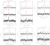 |
Fig. 1 Examples of reduced and calibrated spectra for the NH3 (1, 1), (2, 2) and (3, 3) transitions. The transition is indicated in the upper left corner of each panel. For the first two sources the fits are shown in red. The (3, 3) transition was detected only towards RNO 1B/1C and V512 Per (SVS 13A). The full version of the figure and the FITS files for the NH3 detections are available at https://zenodo.org/record/7736131 |
3.1 Molecular excitation
The rotational (Trot) and kinetic (Tkin) temperatures, as well as the ammonia column density  , were determined using the standard method (Ho & Townes 1983; Ungerechts & Guesten 1984). The results are given in Tables 5 and 6 for the FUors and EXors, respectively.
The rotational temperature can only be determined for sources in which both the (1, 1) and (2, 2) transitions were detected. To calculate the Trot values, we used the following relation (Ho & Townes 1983):
 (1)
(1)
using the optical depth of the (1, 1) main line, τm(1, 1), and the main beam brightness temperatures, TMB, of the (1, 1) and (2, 2) main lines derived from the Gaussian fitting.
The derived rotational temperatures in our sample range from 11 K to 18 K, with an average Trot of 13.2 K.
 (2)
(2)
where Trot(1, 2) is the rotational temperature determined from the (1, 1) and (2, 2) inversion transitions, and 42 K is the energy difference between the (1, 1) and (2, 2) levels. We find that the host environments are characterised by kinetic temperatures of 12–21 K with an average kinetic temperature of 14.6 K, with the highest kinetic temperature found towards RNO 1B/1C. These kinetic temperatures are lower than those found towards Class II sources (26–37 K), but they are similar to low-mass and high-mass dense clumps in early evolutionary stages (e.g. Benson & Myers 1989; Pillai et al. 2006; Zhang et al. 2011; Wienen et al. 2012).
To calculate the ammonia column density, the rotational temperature derived from Eq. (1), Trot(1, 2), the optical depth, τm(1, 1), and the line width, ∆υ(1, 1), of the (1, 1) inversion transition are needed. We calculated the Ntot values using the column density of the (1, 1) level, assuming that the energy levels are populated according to the Boltzmann distribution (see e.g. Rohlfs & Wilson 2004; Wienen et al. 2012). For the calculation of the total column density, we used the relation given by Rohlfs & Wilson (2004), with the assumption that the lowest metastable levels dominate in the population:
 (3)
(3)
where Trot(1, 2) is the rotational temperature, and N(1, 1) is the column density of the (1, 1) level,
 (4)
(4)
where gl, gu are the statistical weights of the lower and the upper levels, Aul is the Einstein coefficient, ν is the frequency in units of GHz, Tex is the excitation temperature of the (1, 1) transition, and ∆υ is the line width in units of km s−1. We used the approximation that  in Eq. (4). Assuming LTE, we used the rotational temperature as the excitation temperature (e.g. Goldsmith & Langer 1999; Wilson et al. 2009). The values for gl, gu, Aul, and ν were taken from the Leiden Atomic and Molecular Database (LAMDA, Schöier et al. 2005).
The average rotational temperature for all sources (with the (1, 1) and the (2, 2) emission detected) was found to be 13.2 K. For sources detected only in the (1, 1) transition, we adopted Trot = 13.2 K in order to estimate their NH3 column densities and abundances. The results are given in Tables 5 and 6 for the FUors and EXors, respectively. Since we find rotational temperatures between 11K and 18 K, we assume an uncertainty for the average rotational temperature of ~30%.
The ammonia column densities in the sample range from 5.2 × 1013 cm−2 (IRAS 06393+0913) to 3.2 × 1015 cm−2 (RNO 1B/1C), with an average of 1.18 × 1015 cm−2 and a median of 1.15 × 1015 cm−2, respectively. In infrared dark clouds (IRDCs), ammonia column densities were found to range from 7.6 × 1014 cm−2 to 6.04 × 1015 cm−2, with an average value of 3 × 1015 cm−2 (Pillai et al. 2006). Approximately 2/3 of our sample (18/28 objects ~64%) falls within this range, with the remaining sources having NH3 column densities lower than observed in IRDCs (see Tables 5 and 6).
NH3 (1, 1) line parameters for the FU Orionis-type objects detected in our survey.
NH3 (1, 1) line parameters for the EX Lupi-type objects detected in our survey.
NH3 (2, 2) and (3, 3) line parameters for the FU Orionis-type objects detected in NH3 (1, 1).
3.2 Beam filling factor
The beam filling factor, η, gives the fraction of the beam filled by the observed emission, and it can be derived from the radiative transfer equation when the excitation temperature and optical depth of the transition can be determined. For ammonia, optical depths can be derived from the HFS fitting, and we assumed local thermodynamic equilibrium (LTE) in order to approximate the excitation temperature (see e.g. Wienen et al. 2012; Condon & Ransom 2016; Yan et al. 2021). We determined the η value for each detected source in our sample using the following equation, with the Rayleigh-Jeans approximation,
 (5)
(5)
where TMB(1, 1) is the main beam brightness temperature of the (1, 1) transition, τ(1, 1) is the optical depth of the (1, 1) main line, and Tbg = 2.73 K. Assuming LTE, we used the rotational temperature as the excitation temperature (e.g. Goldsmith & Langer 1999; Wilson et al. 2009). We found that the η values in our sample range from 0.06 to 0.42 with an average of 0.25 and a median of 0.26 (see Tables 5 and 6).
The low beam filling factors may indicate clumpiness on small scales, which indeed has been revealed by interferometric observations of these ammonia transitions towards dark clouds and high-mass starless cores (see e.g. Olmi et al. 2010; Devine et al. 2011; Ragan et al. 2011). We find no significant differences between the η values in this work compared to those in high-mass clumps by Wienen et al. (2012).
3.3 LSR velocities
Table B.1 presents a comparison of the υLSR results from our NH3(1, 1) observations with published υLSR values from the literature. For most sources, the literature LSR velocities were derived from 12CO and its rarer isotopologues. Where other lines or CO observations of nearby clouds were used, this is noted in brackets in Table B.1.
Our observations have yielded the first systemic υLSR measurements for five sources. Due to the sensitivity of our observations, we are also able to derive more precise LSR values for a number of sources (see Table B.1), which could be helpful for follow-up studies (e.g. comparisons with stellar velocities). The differences between the NH3 (1, 1) velocities and the CO literature values are generally less than 1 km s−1, while the velocities derived from the NH3 (1, 1), (2, 2), and (3, 3) lines agree within the errors of the fits, generally <0.03 km s−1.
3.4 Line widths
The line widths of the (1, 1) inversion transition (where the HFS fitting method was used) range from 0.36 km s−1 to 2.39 km s−1. For the (2, 2) transition (where Gaussian fitting was used), the line widths are between 0.42 km s−1 and 2.55 km s−1. We find that the derived line widths for the (2, 2) transition are broader than those for the (1, 1) transition. The line width ratios, ∆υ(2, 2)/∆υ(1, 1), are between 1.02 and 2.58, with a median of 1.23 and a dispersion of 0.16. This is consistent with previous results that the line widths obtained from hyperfine structure fitting are smaller than those from Gaussian fitting (Wienen et al. 2012). We note that in the following analysis we only use the line width of the (1, 1) transition.
In our sample, RNO 1B/1C and AR 6A/6B have the broadest lines, and both have kinetic temperatures >17K. For RNO 1B/1C, the broad line width may be the result of shock heating and shock-driven turbulence caused by this source’s powerful outflow action (see e.g. Anglada et al. 1994; Quanz et al. 2007a; Bae et al. 2011). In contrast, previous observations suggest that AR 6A/6B does not have a CO outflow (Moriarty-Schieven et al. 2008). Based on its environment (see Fig. C.1), we speculate that its increased line width and elevated kinetic temperature are both caused by turbulence.
The observed line width, ∆υ(1, 1), is related to the velocity dispersion, σobs, as  . The observed line widths or velocity dispersions of the inversion lines have contributions from both thermal and non-thermal motions (e.g. Hacar et al. 2016),
 (6)
(6)
where ∆υth and σth are the thermal line width and velocity dispersion, respectively, and ∆υnt and σnt are the non-thermal line width and velocity dispersion, respectively. The thermal line width and velocity dispersion can be calculated from
 (7)
(7)
where k is the Boltzmann constant, Tkin is the kinetic temperature, and m is the molecular weight of the given molecule, in this case  . According to Eq. (6), the non-thermal motions can be derived by subtracting the thermal motions from the total. The kinetic temperatures derived from ammonia are used to derive thermal line widths for sources with both NH3 (1, 1) and NH3 (2, 2) detections. For sources with only an NH3 (1, 1) detection, we assumed the average kinetic temperature of 14.6 K (derived earlier in Sect. 3.1) to calculate the contribution of thermal motions. The results are listed in Tables 1 and 2. Based on these results, we conclude that the line widths of most sources are dominated by non-thermal contributions.
Once σnt is determined, the Mach number can be derived in order to distinguish between sonic (Ma ≤ 1), transonic (1 < Ma ≤ 2) and supersonic (Ma > 2) environments. When calculating the Mach number, Ma = f(Tkin) = σnt/cs, where cs is the sound speed of the molecular gas; both terms depend on Tkin. Typically, the same Tkin is adopted for evaluating σnt and the sound speed (e.g. Hacar et al. 2016).
We calculated the Mach numbers for all sources with detections of both the (1, 1) and (2, 2) transitions using the values of Tkin derived from our observations; the results are listed in Tables 1 and 2 for FUors and EXors, respectively. Using the average kinetic temperature of 14.6 K, we also derived the Mach numbers for sources with only (1, 1) detections, marked in Tables 1 and 2. We find that ten sources have Mach numbers of <1, indicative of sonic motions, while 13 sources show transonic motions. Finally, five FUors in our sample have Mach numbers higher than two, indicating supersonic environments. Because these five FUors are associated with molecular outflows (see Table 5), their higher Mach numbers may be attributable to turbulence driven by outflow shocks. Interestingly, for the EXors, there is no indication of supersonic environments. It is also worth noting that there are several examples of sources that have Mach numbers <1 despite their being known to host outflows (i.e. V899 Mon, V2495 Cyg, HH 354 IRS, etc.). Our results show that the host environments of most of the eruptive stars in our sample are dominated by sonic and transonic motions on the scales sampled with the Effelsberg beam (~37″), indicating that most eruptive stars reside in rather quiescent host environments.
NH3 (2, 2) and (3, 3) line parameters for the EX Lupi-type objects detected in NH3 (1, 1).
Derived parameters for FU Orionis-type objects detected in NH3 emission.
Derived parameters for EX Lupi-type objects detected in NH3 emission.
3.5 Spectral energy distributions
H2 column densities are needed in order to determine ammonia abundances for the sources in our sample. For seven sources with NH3 (1, 1) detections in our survey, H2 column density and dust temperature maps derived from the Herschel Gould Belt survey (André et al. 2010) were available in the literature. For these sources, we measured column density and dust temperature values for our target sources from the published maps, and these adopted values and the literature references are given in Tables 5 and 6. Where H2 column density and dust temperature maps were available in the literature for sources undetected in NH3 in our survey, we similarly measured values for our target sources and include these in Table A.1.
For the remaining sources with NH3 (1, 1) detections, we derived H2 column density and dust temperature maps using archival Herschel/SPIRE data at 250 μm, 350 μm, and 500 μm3 using the same methods as previous studies (e.g. André et al. 2010; Lin et al. 2017; Elia et al. 2017). Prior to pixel-by-pixel spectral-energy-distribution (SED) fitting, the archival data were convolved to a common angular resolution of 36.″3 (i.e. the beamsize of Herschel/SPIRE at 500 μm), which is comparable to the angular resolution of our ammonia observations, and then projected onto the same grid as the 500 μm data.
Assuming that the SED of the dust emission follows the modified-blackbody model, the flux density, Sν, at the frequency ν can be expressed as
 (8)
(8)
where τν is the optical depth at the frequency ν, Bν(Td) is the Planck function evaluated at the dust temperature Td, and Ω is the solid angle of the beam. The H2 column density,  , is proportional to τν with the following relationship:
 (9)
(9)
where μ is the molecular weight per hydrogen molecule, taken to be 2.8 (Kauffmann et al. 2008), κν is the dust opacity per unit (dust+gas) mass, and mH is the mass of hydrogen. The dust opacity per unit mass, κν, is approximated by the power law κν = 0.1(ν/1000GHz)βcm2/g (e.g. Hildebrand 1983), where β is the dust emissivity index, and the canonical gas-to-dust ratio of 100 has been applied. Following previous studies (e.g. André et al. 2010; Elia et al. 2017), β is assumed to be two here. The SED fitting was performed using the ‘LMFIT’4 python package (Newville et al. 2014) to fit the two free parameters,  and Td, for every pixel. The results are shown in Fig. C.1, and the corresponding beam-averaged values are given in Tables 5 and 6.
For sources in our sample with NH3 (1, 1) detections, the dust temperatures range from 11.8 K to 21.8 K and the derived H2 column densities range from 9.0 × 1021 cm−2 to 2.2 × 1023 cm−2. We compared the dust temperatures and gas kinetic temperatures for sources in our sample with Tkin measurements (i.e. those with both NH3 (1, 1) and (2, 2) detections), and found that in most cases the dust temperature and gas kinetic temperature agree within 3 K. The only exception is RNO 1B/1C, which has a gas kinetic temperature that is much higher than its dust temperature (Tkin = 21.3 K, Td = 14.5 K). Such a scenario could be caused by inefficient gas-to-dust coupling and gas cooling if the density was < 103.5 cm−3 (Goldsmith 2001). However, RNO 1B/1C is surrounded by deeply embedded objects, forming a small cluster (Quanz et al. 2007a). Based on the dust temperature map of the source (see Fig. C.1) there is significantly warmer dust within <1′ of the source position, and this warmer material likely contributes to the higher temperature measured in the Effelsberg beam.
Interestingly, based on the derived H2 column density maps (Fig. C.1), we find that the host environments of the eruptive stars detected in NH3 (1, 1) are quite diverse on scales larger than the Effelsberg beam (~37″). A few sources are relatively isolated, while others are associated with larger, extended cloud structures.
3.6 Ammonia abundance
We used the NH3 and H2 column densities from Sects. 3.1 and 3.5, respectively, to derive ammonia abundances:  . The derived abundances, listed in Tables 5 and 6, range from 4.7 × 10⁻⁹ to 1.5 × 10⁻⁷, with an average of 3.6 × 10⁻⁸ and a median of 2.8 × 10⁻⁸, respectively.
We compare our results with the NH3 abundances found in other studies, including low-mass, intermediate-mass, and highmass star-forming regions. Our derived NH3 abundances are similar to values found in cold, dark clouds (see e.g. Ohishi et al. 1992). With very few exceptions, our derived NH3 abundances fall within the range observed towards IRDCs (e.g. 0.7 × 10⁻⁸ to 15.9 × 10⁻⁸; Pillai et al. 2006; Zhang et al. 2011). The exceptions are NGC 2071 and IRAS 06393+0913, which have abundances of −0.6 × 10⁻⁸ and −0.5 × 10⁻⁸, respectively (see Table 5.) Our average abundance of 3.6 × 10⁻⁸ is also similar to the average values reported for IRDCs by Pillai et al. (2006) (−4 × 10⁻⁸) and for high-mass clumps by Dunham et al. (2011) (4.6 × 10⁻⁸). Interestingly, NH3 abundances observed towards Herbig Ae/Be stars, which are intermediate-mass pre-main-sequence stars, range from 1 × 10⁻⁸ to 4 × 10⁻⁸ (Fuente et al. 1990); this is on the lower end of the range observed towards IRDCs and towards our sample.
4 Discussion
4.1 Ammonia in the neighbourhood of outbursting systems
Based on previous studies, ammonia emission can have different origins, corresponding to grain surface and gas-phase chemistry (see Jørgensen et al. 2020, and references therein, for the most recent review). In the following, we compare our observations with these different scenarios. We first discuss ammonia release from grains, and then we examine the formation of NH3 via gasphase chemistry.
During an outburst, the whole disc experiences a temperature increase due to the energy released in the very inner few 0.1 au of the disc (e.g. Fischer et al. 2022). The temperature increase in the outer part of the disc could easily sublimate ammonia molecules off the grains, releasing them back into the gas phase (Guesten & Fiebig 1988) and enhancing the ammonia abundance. However, any ammonia set free in this way should not make a significant contribution to our observed ammonia emission; this is because our FWHM beam size of ~37″ (i.e. 5000 au at 140 pc) is much larger than typical disc sizes (~60 au; Maury et al. 2019), beam dilution effects should result in only a very minor contribution to the ammonia signals we observe. Such enhancements would be better constrained with higher angular resolution observations of ammonia transitions towards the discs around eruptive stars, especially during the bursting phase.
Alternatively, chemical models suggest that ammonia molecules on dust grains can be released into the gas phase through the passage of shocks produced by molecular outflows (e.g. Holdship et al. 2017). Such effects have already been confirmed by observations of outflows (e.g. Tafalla & Bachiller 1995; Umemoto et al. 1999; Feng et al. 2022) and could explain the relatively high ammonia abundances in some sources, such as RNO 1B/1C. In fact, almost all of the sources in our sample with ammonia (1, 1) detections possess CO outflows (see Tables 5 and 6).
As suggested by early studies (e.g. Herbst & Klemperer 1973; Galloway & Herbst 1989), ammonia can also form in cold molecular gas via successive hydrogenation of N+ by H2 and the subsequent electron recombination of  . Hence, it is also possible that the observed ammonia emission is dominated by circumstellar envelopes and/or ambient clouds; as discussed in Sect. 3.6, we find that the eruptive stars in our sample generally have NH3 abundances similar to those of IRDCs. A circumstellar envelope is an important part of any YSO system as it is a reservoir of material, replenishing a disc with matter (e.g. Hartmann & Kenyon 1996). For example, previous observations of a deeply embedded Class 0 protostar suggest that the ammonia emission is dominated by the circumstellar envelopes on scales of 104 au, revealed from interferometric observations (Tanner & Arce 2011; Jhan & Lee 2021). Based on Fig. C.1, we find that CB 230, HH 354 IRS, L1551 IRS 5, PP 13S, RNO 1B/1C, V960 Mon, and V1057 Cyg coincide with dense dust concentrations, which is indicative of the presence of dense circumstellar envelopes. In several cases, our observations are the first NH3 detections of dense circumstellar envelopes identified in other datasets. The dense circumstellar envelopes of RNO 1B/1C and V1057 Cyg have been confirmed by an interferometric 13CO and C18O survey (Fehér et al. 2017), with further evidence for an envelope in V1057 Cyg from its SED, using the extensive multi-wavelength data available for this source (Szabó et al. 2021). Similarly, we detect NH3 (1, 1) and (2, 2) towards the EXor type object V371 Ser (also known as EC 53), which is known to have a dense circumstellar envelope based on millimetre observations and radiative transfer modelling (e.g. Baek et al. 2020; Lee et al. 2020, and references therein).
Our new ammonia detections, combined with the Herschel column density maps, suggest that V2492 Cyg and V2495 Cyg are also associated with dense material. However, we note that it is clear they do not possess the highest column densities or most concentrated peaks. In the case of AR 6A/6B, our NH3 (1, 1) and (2, 2) detections are tentative evidence of the presence of dense gas. In the H2 column density map (Fig. C.1), however, the dust concentrations appear offset from the target source. Kóspál et al. (2017) found that the CO emission peak at υLSR = 5.3 km s−1 (similar to the 5.06 km s−1 derived from the ammonia (1, 1) transition) was offset from AR 6A/6B, and suggested, based on the Herschel/SPIRE 250 μm image, that this source lies in a cavity. Based on these results and our H2 column density map (Fig. C.1), it is most likely that the NH3 emission picked up by the Effelsberg beam originates from material offset from the source. For other sources with NH3 detections but without associated dense dust concentration, their ammonia emission might arise from ambient clouds.
The non-detections of ammonia transitions in our survey could indicate that dense circumstellar envelopes are not present or that the objects are too far away for their envelopes to be detected. The distances are known for the majority of sources in our sample (e.g. Audard et al. 2014), allowing us to investigate the second possibility. Interestingly, RNO 1B/1C is the farthest source in our sample, yet NH3 emission was still detected in multiple transitions. Similarly, at least NH3 (1, 1) was detected towards other sources with large distances, such as Z CMa, V1735 Cyg and V2495 Cyg, suggesting that distance is unlikely to be a main explanation for NH3 non-detections. Instead, the non-detections may indicate that dense circumstellar envelopes have already been dispersed. For instance, the ammonia non-detection in the case of V1515 Cyg is consistent with a recent multi-wavelength SED analysis that found no clear sign of a massive circumstellar envelope (Szabó et al. 2022).
4.2 The reliability of the standard classification scheme for outbursting systems
Based on the standard classification scheme (e.g. Greene et al. 1994; Evans et al. 2009), the sources in our sample have been classified as Class I, Class II, or transition objects (i.e. Class 0/I or Class I/II, see Table B.1). Because Class II objects are thought to be beyond the embedded phase (see Fischer et al. 2022, and references therein, for the most recent review), their host environments are not expected to harbour as much dense gas as those of younger sources. In our sample, the Class 0/I and Class I sources have the highest ammonia detection rates: 16 sources (3 Class 0/I and 13 Class I) are detected in NH3 (1, 1), corresponding to detection rates of 100% for Class 0/I sources and 81% for Class I sources. Seven of these sources are also detected in NH3 (2, 2). Notably, however, we also detect NH3 (1, 1) towards nine sources classified as older than Class I, 4 of which are also detected in (2, 2) emission. We detect ammonia towards 1 Class I/II and 8 Class II objects in our survey, corresponding to detection rates of 33% and 47%, respectively. We also note that some of the Class II sources (namely HBC 722, V1057 Cyg, V1735 Cyg, and RNO 1B/1C) have higher NH3 and H2 column densities than some sources classified as Class I or Class 0/I or Class I/II transition objects.
Our results show that, as expected, the younger systems have significantly higher ammonia detection rates. However, based on the dust and ammonia evidence, some sources classified as older systems, that are Class II sources, can still be associated with high concentrations of their dense cores, which is indicative of a younger evolutionary stage. Interestingly, it is puzzling that many younger sources were not detected in our survey (see Table B.1). We emphasise the need for future interferometric studies to better understand the effects of the outbursts on the dense cores of young eruptive stars. Higher-angular resolution NH3 observations could potentially probe whether there is a connection and/or ongoing accretion from cloud and/or filament down to core scales (e.g. Redaelli et al. 2022), since NH3 can be used to identify the presence of dense gas.
As already proposed by Quanz et al. (2007b), the standard classification scheme for low-mass YSOs might not be able to adequately classify FUors, since they might represent an inter-evolutionary stage in the standard classification scheme. Furthermore, FUors might undergo several outburst events (Herbig 1977; Hartmann & Kenyon 1985), just like EXors. After several outbursts, the envelope vanishes in about several hundred thousand years (as discussed above: supplying the accretion disc with more material; e.g. Fischer et al. 2022). As a consequence, the objects enter a permanent low accretion state (i.e. they become T Tauri stars), as discussed by Takami et al. (2018, 2019). Weintraub et al. (1991) and Sandell & Weintraub (2001) also suggest that FUors are younger than T Tauri stars and might be an important link between the more embedded Class I and the more evolved Class II stages (the latter closer to or being T Tauri stars.) Additionally, some FUors have features of both Class I and Class II sources; these include warm continuum consistent with Class II sources, but rotational line emission typical of Class I, which is far higher than Class II sources with a similar mass/luminosity (Green et al. 2013).
Compared to the later evolutionary stages, one of the important features of the embedded phase is the presence of dense circumstellar envelopes around YSOs. The appearance of the 10 μm silicate feature in absorption has been regarded as a signature for such a circumstellar envelope (Quanz et al. 2007b), and dust continuum emission also traces the cold envelopes around YSOs. Molecular line tracers such as ammonia can provide another tool to investigate the surrounding environments. Because the effective critical densities of the NH3 (1, 1) and (2, 2) lines are 7.9 × 102 cm−3 and 1.6 × 104 cm−3, respectively, the detection of NH3 (1, 1) and (2, 2) would suggest the presence of dense gas at a H2 density of ~ 1 × 104 cm−3 (Shirley 2015), which would in turn indicate the embedded phase. The presence of dense gas (~ 1 × 104 cm−3) indicates that some of the eruptive stars in our sample lie at an earlier phase than previously classified (see Table B.1). For instance, our result from the ammonia observations agrees well with previous studies on V371 Ser (EXor), which was classified as a Class I object based on its spectral index and bolometric temperature (e.g. Dunham et al. 2015), but ALMA observations revealed that its envelope has a much higher mass than its disc and protostar, suggesting that the source might actually be a Class 0 object (Lee et al. 2020). We suggest that incorporating more data regarding the presence of dense material surrounding these peculiar objects into the standard classification scheme could better illuminate the evolutionary stages of eruptive FUors and EXors.
By the original definition, the young eruptive star classes of FUors and EXors are Class II objects, and therefore they are T Tauri stars (see e.g. Adams et al. 1987; Lada 1987; Kenyon & Hartmann 1991; Hartmann & Kenyon 1996). This was further suggested by the only available pre-outburst spectra for two FUors: V1057 Cyg and HBC 722, which both showed properties reminiscent of classical T Tauri stars (CTTS) prior to their outbursts (Herbig 1977; Miller et al. 2011). However, nowadays there are many examples of more embedded young eruptive stars, which were also part of our sample, i.e. Haro 5a IRS, HH 354 IRS, L1551 IRS 5 (see e.g. Audard et al. 2014; Connelley & Reipurth 2018).
Apart from a single dish study by Lang & Willson (1979), there are no dedicated surveys investigating the dense environments specifically focusing only on T Tauri stars, the closest objects to the ones in our study. The sample of Lang & Willson (1979) consisted of 34 T Tauri stars located in Taurus-Auriga and the young star cluster NGC 2264, which is accessible with the Arecibo telescope. Out of the 34 sources they detected at least the (1, 1) transition toward 13 sources, equivalent to a detection rate of 38%. In our case, the sample consisted of 17 Class II sources (see Table B.1), and we have detected at least the (1, 1) transition toward 8 of them, which is ~47%. Lang & Willson (1979) found kinetic temperatures from 26 K to 37 K, and column densities between 1 and 5.9 × 1014 cm−2. In our sample, the Class II sources (see Table B.1) have kinetic temperatures between 13.63 K and 21.35 K and column densities from 1.3 × 1014 cm−2 to 1.8 × 1015 cm−2. When compared to Lang & Willson (1979), we found that for a few of the Class II sources, namely V899 Mon and V960 Mon, the column densities are within the same order of magnitude, i.e., ~1014 cm−2. However, there are other Class II sources that have ~1 order of magnitude higher column density values (i.e., ~ 1015 cm−2), namely RNO 1B/1C, AR 6A/6B, HBC 722, V1057 Cyg, and V1735 Cyg. The similar column densities suggest that ammonia does not probe the part of the envelope impacted by the outburst.
We also compared our results to NH3 observations of Herbig Ae/Be stars, YSOs that are the intermediate mass counterparts of T Tauri stars (see e.g. Waters & Waelkens 1998). These YSOs have similar properties to the objects in our sample, such as P Cygni profiles indicating mass loss (Strom et al. 1972) and stellar winds (Canto et al. 1984), and they are usually illuminating nebulosities (just as the first few FUor examples) (Herbig 1960); however, outflows are more typical and better understood in low-mass YSOs (e.g. Pezzuto et al. 1997; Tambovtseva & Grinin 2016; Fischer et al. 2022). Fuente et al. (1990) found ammonia column densities ranging between 0.5 × 10¹⁴ and 2.9 × 1014 cm−2, which are within the same range for five sources (NGC 2071, V899 Mon, IRAS 06393+0913, V960 Mon, and Z CMa) in our sample (see Tables 5 and 6). In their study, Fuente et al. (1990) also obtained maps and found that in HD 200775, a source illuminating an extended reflection nebula in NGC 7023, three different clumps could be traced with the NH3 emission, with varying rotational temperatures and column densities. High angular resolution observations in the future of a selected sample of eruptive objects could reveal similar clumpiness of the ammonia emission in the host environments of FUors and EXors.
5 Conclusions
In this paper, we present the results of the first dedicated ammonia survey of low-mass, young eruptive stars to investigate their host environments. Our sample included a total of 51 objects, including FUors, EXors, and Gaia alerts, the latter of which are yet to be classified. Our observations using the Effelsberg 100-m radio telescope resulted in the detection of NH3 (1, 1) in 28 sources (24 FUors, 4 EXors), NH3 (2, 2) in 12 sources (10 FUors, 2 EXors), and NH3 (3, 3) in two sources (the FUor-type object RNO 1B/1C and the EXor-type object V512 Per, the latter more commonly known as SVS 13). Ammonia emission was not detected towards any of the Gaia alert sources. Our analysis leads to the following conclusions:
Based on the results for the 12 sources with both NH3 (1, 1) and NH3 (2, 2) detections the kinetic temperatures range from ~12K to ~21K, which is slightly lower than the Tkin values reported towards classical T Tauri stars. The ammonia column densities for sources in our sample detected in NH3 (1, 1) range from 5.2 × 1013 cm−2 to 3.2 × 1015 cm−2. The average value for our sample, 1.18 × 1015 cm−2, is higher than the ammonia column densities found towards T Tauri stars. The ammonia abundances with respect to H2 for our sample range from 4.7 × 10⁻⁹ to 1.5 × 10⁻⁷ with an average of 3.6 × 10⁻⁸ and a median of 2.8 × 10⁻⁸, comparable to IRDCs.
Most of the eruptive stars in our sample reside in rather quiescent (sonic or transonic) host environments, with the exception of five FUors (RNO 1B/1C, Haro 5a IRS, AR 6A/6B, Z CMa and HBC 722) that exhibit supersonic motions. The supersonic motions might be caused by associated outflows.
We investigated the origin of the observed ammonia emission in the outbursting systems. Comparing with dust-based H2 column density maps, we find that circumstellar envelopes are present and likely contribute to the observed ammonia emission in seven sources: CB 230, HH 354 IRS, L1551 IRS 5, PP 13S, RNO 1B/1C, V960 Mon, and V1057 Cyg. Outflow shocks could contribute to the relatively high ammonia abundances in sources such as RNO 1B/1C.
Additional eruptive stars potentially harbour dense gas based on their NH3 (2, 2) detections, which could indicate an earlier phase than originally classified. Our results add to the growing evidence that low-mass, young eruptive stars occupy a wide range of evolutionary stages (see also Green et al. 2013).
Our Effelsberg ammonia observations assisted our investigation of the host environments of eruptive low-mass stars on scales of ~37″, much larger than the discs surrounding our targets (e.g. Cieza et al. 2018; Kóspál et al. 2021; Liu et al. 2021). For the majority of these young eruptive stars, their environments are still poorly constrained on small scales, and further high angular resolution observations are needed to shed light on the relationship between young eruptive stars, their discs, and their potential circumstellar envelopes.
Such observations will be important for expanding the standard classification scheme of YSOS, and for studying the effects of the outburst on the host environments of young eruptive stars.
Acknowledgements
Based on observations (Project ID: 95-21, PI: Szabó) with the 100-m telescope of the MPIfR (Max-Planck-Institut für Radioastronomie) at Effelsberg. Zs.M.Sz. acknowledges funding from a St Leonards scholarship from the University of St Andrews. For the purpose of open access, the author has applied a Creative Commons Attribution (CC BY) licence to any Author Accepted Manuscript version arising. This research has made use of data from the Herschel Gould Belt survey (HGBS) project (http://gouldbelt-herschel.cea.fr). The HGBS is a Herschel Key Programme jointly carried out by SPIRE Specialist Astronomy Group 3 (SAG 3), scientists of several institutes in the PACS Consortium (CEA Saclay, INAF-IFSI Rome and INAF-Arcetri, KU Leuven, MPIA Heidelberg), and scientists of the Herschel Science Center (HSC). This project has received funding from the European Research Council (ERC) under the European Union’s Horizon 2020 research and innovation programme under grant agreement No. 716155 (SACCRED).
Appendix A Sources with non-detections
In Table A.1, we list 3σ upper limits for sources without ammonia detections. Gaia alerts were chosen based on their light curves and luminosities at the time of our proposal submission. These objects were chosen because their light curves resembled those of FUors and EXors. Interestingly, no ammonia was detected towards any of the Gaia alert sources.
Sources without ammonia detections in our survey.
Appendix B Classification and υLSR
In Table B.1, we list all FUors and EXors from our sample including both ammonia detections and non-detections. We tabulate whether each source is an FUor or EXor and previously determined υLSR velocities, with the line(s) used to determine these velocities noted in brackets (a dash indicates no available data). We also list the υLSR results from our ammonia observations, where a dash indicates a non-detection. We list classifications if available in the literature and give the references. Finally in the last column we give the distances if available, which, except for RNO 1B/1C, V512 Per, Z CMa, and HH 354 IRS, are adopted from the study of Audard et al. (2014). For these four sources we used updated distances, because of water maser detections associated with these sources in our Paper II. In the case of V512 Per (more commonly known as SVS 13), the source is a resolved binary, consisting of VLA 4A and 4B (e.g. Diaz-Rodriguez et al. 2022). We found CO line data for both sources, from which we find an average value of 8.35 km s−1, similar to our unresolved single-dish result.
Reference classification and υLSR for the FUors and EXors in our sample, including NH3 detections and non-detections.
Appendix C H2 column density and dust temperature maps
Figure C.1 shows the H2 column density and dust temperature maps derived from the SED fitting described in Sect. 3.5. The H2 column density and dust temperature values are listed in Tables 5 and 6.
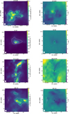 |
Fig. C.1 H2 column density (left) and dust temperature (right) maps derived from the pixel-by-pixel SED fitting of the Herschel data, convolved to the Effelsberg beam (shown in the bottom left corner). The field of view is the same for all sources, corresponding to 10′ × 10′, and + symbols represent the pointing positions listed in Tables 1, 2 and B.1, respectively. The physical scale is presented for sources with known distances, taken from the study of Audard et al. (2014) or described in the notes of Table B.1. The colour scale is not the same for all sources. |
References
- Ábrahám, P., Kóspál, Á., Csizmadia, S., et al. 2004, A & A, 428, 89 [CrossRef] [EDP Sciences] [Google Scholar]
- Ábrahám, P., Kóspál, Á., Kun, M., et al. 2018, ApJ, 853, 28 [CrossRef] [Google Scholar]
- Adams, F. C., Lada, C. J., & Shu, F. H. 1987, ApJ, 312, 788 [NASA ADS] [CrossRef] [Google Scholar]
- ALMA Partnership (Brogan, C. L., et al.) et al. 2015, ApJ, 808, L3 [Google Scholar]
- André, P., Men’shchikov, A., Bontemps, S., et al. 2010, A & A, 518, A102 [Google Scholar]
- Anglada, G., Rodriguez, L. F., Girart, J. M., Estalella, R., & Torrelles, J. M. 1994, ApJ, 420, L91 [CrossRef] [Google Scholar]
- Arzoumanian, D., André, P., Didelon, P., et al. 2011, A & A, 529, L6 [NASA ADS] [CrossRef] [EDP Sciences] [Google Scholar]
- Audard, M., Ábrahám, P., Dunham, M. M., et al. 2014, in Protostars and Planets VI, eds. H. Beuther, R. S. Klessen, C. P. Dullemond, & T. Henning, 387 [Google Scholar]
- Bae, J.-H., Kim, K.-T., Youn, S.-Y., et al. 2011, ApJS, 196, 21 [NASA ADS] [CrossRef] [Google Scholar]
- Baek, G., MacFarlane, B. A., Lee, J.-E., et al. 2020, ApJ, 895, 27 [Google Scholar]
- Bailer-Jones, C. A. L., Rybizki, J., Fouesneau, M., Demleitner, M., & Andrae, R. 2021, AJ, 161, 147 [Google Scholar]
- Banzatti, A., Meyer, M. R., Manara, C. F., Pontoppidan, K. M., & Testi, L. 2014, ApJ, 780, 26 [Google Scholar]
- Bell, K. R., Lin, D. N. C., Hartmann, L. W., & Kenyon, S. J. 1995, ApJ, 444, 376 [NASA ADS] [CrossRef] [Google Scholar]
- Benson, P. J., & Myers, P. C. 1989, ApJS, 71, 89 [Google Scholar]
- Borchert, E. M. A., Price, D. J., Pinte, C., & Cuello, N. 2022, MNRAS, 510, L37 [Google Scholar]
- Bronfman, L., Nyman, L. A., & May, J. 1996, A & AS, 115, 81 [NASA ADS] [Google Scholar]
- Canto, J., Rodriguez, L. F., Calvet, N., & Levreault, R. M. 1984, ApJ, 282, 631 [NASA ADS] [CrossRef] [Google Scholar]
- Cao, Y., Qiu, K., Zhang, Q., et al. 2019, ApJS, 241, 1 [Google Scholar]
- Chen, X., Launhardt, R., & Henning, T. 2007, ApJ, 669, 1058 [NASA ADS] [CrossRef] [Google Scholar]
- Cheung, A. C., Rank, D. M., Townes, C. H., Thornton, D. D., & Welch, W. J. 1968, Phys. Rev. Lett., 21, 1701 [NASA ADS] [CrossRef] [Google Scholar]
- Cieza, L. A., Ruíz-Rodríguez, D., Perez, S., et al. 2018, MNRAS, 474, 4347 [CrossRef] [Google Scholar]
- Clarke, C. J., Lodato, G., Melnikov, S. Y., & Ibrahimov, M. A. 2005, MNRAS, 361, 942 [NASA ADS] [CrossRef] [Google Scholar]
- Condon, J. J., & Ransom, S. M. 2016, Essential Radio Astronomy (Princeton: Princeton University Press) [Google Scholar]
- Connelley, M. S., & Greene, T. P. 2010, AJ, 140, 1214 [Google Scholar]
- Connelley, M. S., & Reipurth, B. 2018, ApJ, 861, 145 [NASA ADS] [CrossRef] [Google Scholar]
- Cruz-Sáenz de Miera, F., Kóspál, Á., Ábrahám, P., et al. 2022, ApJ, 927, 125 [CrossRef] [Google Scholar]
- Cruz-Sáenz de Miera, F., Kóspál, Á., Ábrahám, P., et al. 2023, ApJ, 945, 80 [CrossRef] [Google Scholar]
- Devine, K. E., Chandler, C. J., Brogan, C., et al. 2011, ApJ, 733, 44 [NASA ADS] [CrossRef] [Google Scholar]
- Diaz-Rodriguez, A. K., Anglada, G., Blázquez-Calero, G., et al. 2022, ApJ, 930, 91 [NASA ADS] [CrossRef] [Google Scholar]
- Di Francesco, J., Keown, J., Fallscheer, C., et al. 2020, ApJ, 904, 172 [NASA ADS] [CrossRef] [Google Scholar]
- Dong, R., Liu, H. B., Cuello, N., et al. 2022, Nat. Astron., 6, 331 [NASA ADS] [CrossRef] [Google Scholar]
- Dunham, M. K., Rosolowsky, E., Evans I., Neal J., Cyganowski, C., & Urquhart, J. S. 2011, ApJ, 741, 110 [NASA ADS] [CrossRef] [Google Scholar]
- Dunham, M. M., Allen, L. E., Evans, I., Neal J., et al. 2015, ApJS, 220, 11 [NASA ADS] [CrossRef] [Google Scholar]
- Elia, D., Molinari, S., Schisano, E., et al. 2017, MNRAS, 471, 100 [NASA ADS] [CrossRef] [Google Scholar]
- Evans I., Neal J., Balkum, S., Levreault, R. M., Hartmann, L., & Kenyon, S. 1994, ApJ, 424, 793 [NASA ADS] [CrossRef] [Google Scholar]
- Evans, I., Neal J., Dunham, M. M., Jørgensen, J. K., et al. 2009, ApJS, 181, 321 [NASA ADS] [CrossRef] [Google Scholar]
- Fehér, O., Kóspál, Á., Ábrahám, P., Hogerheijde, M. R., & Brinch, C. 2017, A & A, 607, A39 [CrossRef] [EDP Sciences] [Google Scholar]
- Feng, S., Liu, H. B., Caselli, P., et al. 2022, ApJ, 933, L35 [CrossRef] [Google Scholar]
- Fiorellino, E., Elia, D., André, P., et al. 2021, MNRAS, 500, 4257 [Google Scholar]
- Fischer, W. J., Hillenbrand, L. A., Herczeg, G. J., et al. 2022, arXiv e-prints, [arXiv:2203.11257] [Google Scholar]
- Fuente, A., Martin-Pintado, J., Cernicharo, J., & Bachiller, R. 1990, A & A, 237, 471 [NASA ADS] [Google Scholar]
- Fuller, G. A., Ladd, E. F., Padman, R., Myers, P. C., & Adams, F. C. 1995, ApJ, 454, 862 [NASA ADS] [CrossRef] [Google Scholar]
- Galloway, E. T., & Herbst, E. 1989, A & A, 211, 413 [NASA ADS] [Google Scholar]
- Giannini, T., Lorenzetti, D., Antoniucci, S., et al. 2016, ApJ, 819, L5 [CrossRef] [Google Scholar]
- Goldsmith, P. F. 2001, ApJ, 557, 736 [Google Scholar]
- Goldsmith, P. F., & Langer, W. D. 1999, ApJ, 517, 209 [Google Scholar]
- Gramajo, L. V., Rodón, J. A., & Gómez, M. 2014, AJ, 147, 140 [NASA ADS] [CrossRef] [Google Scholar]
- Greene, T. P., Wilking, B. A., Andre, P., Young, E. T., & Lada, C. J. 1994, ApJ, 434, 614 [NASA ADS] [CrossRef] [Google Scholar]
- Green, J. D., Evans, I., Neal J., Kóspál, Á., et al. 2013, ApJ, 772, 117 [CrossRef] [Google Scholar]
- Guesten, R., & Fiebig, D. 1988, A & A, 204, 253 [NASA ADS] [Google Scholar]
- Hacar, A., Alves, J., Burkert, A., & Goldsmith, P. 2016, A & A, 591, A104 [NASA ADS] [CrossRef] [EDP Sciences] [Google Scholar]
- Hartmann, L., & Kenyon, S. J. 1985, ApJ, 299, 462 [CrossRef] [Google Scholar]
- Hartmann, L., & Kenyon, S. J. 1996, ARA & A, 34, 207 [NASA ADS] [CrossRef] [Google Scholar]
- Harvey, P. M., Huard, T. L., Jørgensen, J. K., et al. 2008, ApJ, 680, 495 [NASA ADS] [CrossRef] [Google Scholar]
- Herbig, G. H. 1960, ApJS, 4, 337 [Google Scholar]
- Herbig, G. H. 1977, ApJ, 217, 693 [NASA ADS] [CrossRef] [Google Scholar]
- Herbig, G. H. 1989, in European Southern Observatory Conference and Workshop Proceedings, 33, European Southern Observatory Conference and Workshop Proceedings, 233 [NASA ADS] [Google Scholar]
- Herbig, G. H. 1990, ApJ, 360, 639 [NASA ADS] [CrossRef] [Google Scholar]
- Herbst, E., & Klemperer, W. 1973, ApJ, 185, 505 [Google Scholar]
- Hildebrand, R. H. 1983, QJRAS, 24, 267 [NASA ADS] [Google Scholar]
- Hillenbrand, L. A., Miller, A. A., Covey, K. R., et al. 2013, AJ, 145, 59 [NASA ADS] [CrossRef] [Google Scholar]
- Hillenbrand, L. A., Contreras Peña, C., Morrell, S., et al. 2018, ApJ, 869, 146 [NASA ADS] [CrossRef] [Google Scholar]
- Hillenbrand, L. A., Reipurth, B., Connelley, M., Cutri, R. M., & Isaacson, H. 2019, AJ, 158, 240 [NASA ADS] [CrossRef] [Google Scholar]
- Ho, P. T. P., & Townes, C. H. 1983, ARA & A, 21, 239 [NASA ADS] [CrossRef] [Google Scholar]
- Holdship, J., Viti, S., Jiménez-Serra, I., Makrymallis, A., & Priestley, F. 2017, AJ, 154, 38 [NASA ADS] [CrossRef] [Google Scholar]
- Jhan, K.-S., & Lee, C.-F. 2021, ApJ, 909, 11 [NASA ADS] [CrossRef] [Google Scholar]
- Jørgensen, J. K., Belloche, A., & Garrod, R. T. 2020, ARA & A, 58, 727 [CrossRef] [Google Scholar]
- Jurdana-Šepić, R., Munari, U., Antoniucci, S., Giannini, T., & Lorenzetti, D. 2018, A & A, 614, A9 [CrossRef] [EDP Sciences] [Google Scholar]
- Kadam, K., Vorobyov, E., Regály, Z., Kóspál, Á., & Ábrahám, P. 2020, ApJ, 895, 41 [NASA ADS] [CrossRef] [Google Scholar]
- Kauffmann, J., Bertoldi, F., Bourke, T. L., Evans, N. J. I., & Lee, C. W. 2008, A & A, 487, 993 [NASA ADS] [CrossRef] [EDP Sciences] [Google Scholar]
- Kenyon, S. J., & Hartmann, L. W. 1991, ApJ, 383, 664 [NASA ADS] [CrossRef] [Google Scholar]
- Kenyon, S. J., Hartmann, L., & Hewett, R. 1988, ApJ, 325, 231 [NASA ADS] [CrossRef] [Google Scholar]
- Klein, B., Hochgürtel, S., Krämer, I., et al. 2012, A & A, 542, A3 [Google Scholar]
- Könyves, V., André, P., Arzoumanian, D., et al. 2020, A & A, 635, A34 [CrossRef] [EDP Sciences] [Google Scholar]
- Kóspál, Á., Ábrahám, P., Prusti, T., et al. 2006, in Astronomical Society of the Pacific Conference Series, 349, Astrophysics of Variable Stars, eds. C. Aerts & C. Sterken, 269 [Google Scholar]
- Kóspál, Á., Ábrahám, P., Apai, D., et al. 2008, MNRAS, 383, 1015 [CrossRef] [Google Scholar]
- Kóspál, Á., Ábrahám, P., Acosta-Pulido, J. A., et al. 2011, A & A, 527, A133 [CrossRef] [EDP Sciences] [Google Scholar]
- Kóspál, Á., Ábrahám, P., Moór, A., et al. 2015, ApJ, 801, L5 [CrossRef] [Google Scholar]
- Kóspál, Á., Ábrahám, P., Acosta-Pulido, J. A., et al. 2016, A & A, 596, A52 [CrossRef] [EDP Sciences] [Google Scholar]
- Kóspál, Á., Ábrahám, P., Csengeri, T., et al. 2017, ApJ, 836, 226 [CrossRef] [Google Scholar]
- Kóspál, Á., Cruz-Sáenz de Miera, F., White, J. A., et al. 2021, ApJS, 256, 30 [CrossRef] [Google Scholar]
- Lada, C. J. 1987, in Star Forming Regions, 115, eds. M. Peimbert, & J. Jugaku, 1 [NASA ADS] [Google Scholar]
- Lang, K. R., & Willson, R. F. 1979, ApJ, 227, 163 [NASA ADS] [CrossRef] [Google Scholar]
- Lee, S., Lee, J.-E., Aikawa, Y., Herczeg, G., & Johnstone, D. 2020, ApJ, 889, 20 [NASA ADS] [CrossRef] [Google Scholar]
- Lin, D. N. C., & Papaloizou, J. 1985, in Protostars and Planets II, eds. D. C. Black, & M. S. Matthews, 981 [Google Scholar]
- Lin, Y., Liu, H. B., Dale, J. E., et al. 2017, ApJ, 840, 22 [CrossRef] [Google Scholar]
- Liu, H. B., Dunham, M. M., Pascucci, I., et al. 2018, A & A, 612, A54 [NASA ADS] [CrossRef] [EDP Sciences] [Google Scholar]
- Liu, H. B., Tsai, A.-L., Chen, W. P., et al. 2021, ApJ, 923, 270 [NASA ADS] [CrossRef] [Google Scholar]
- Mathieu, R. D., Martin, E. L., & Magazzu, A. 1996, in American Astronomical Society Meeting Abstracts, 188, American Astronomical Society Meeting Abstracts #188, 60.05 [Google Scholar]
- Maury, A. J., André, P., Testi, L., et al. 2019, A & A, 621, A76 [NASA ADS] [CrossRef] [EDP Sciences] [Google Scholar]
- Miller, A. A., Hillenbrand, L. A., Covey, K. R., et al. 2011, ApJ, 730, 80 [NASA ADS] [CrossRef] [Google Scholar]
- Miller, A. A., Hillenbrand, L. A., Bilgi, P., et al. 2015, The Astronomer’s Telegram, 7428, 1 [Google Scholar]
- Moriarty-Schieven, G. H., Aspin, C., & Davis, G. R. 2008, AJ, 136, 1658 [NASA ADS] [CrossRef] [Google Scholar]
- Nagy, Z., Szegedi-Elek, E., Ábrahám, P., et al. 2021, MNRAS, 504, 185 [NASA ADS] [CrossRef] [Google Scholar]
- Nagy, Z., Ábrahám, P., Kóspál, Á., et al. 2022, MNRAS, 515, 1774 [NASA ADS] [CrossRef] [Google Scholar]
- Newville, M., Stensitzki, T., Allen, D. B., & Ingargiola, A. 2014, LMFIT: NonLinear Least-Square Minimization and Curve-Fitting for Python [Google Scholar]
- Ohishi, M., Irvine, W. M., & Kaifu, N. 1992, in Astrochemistry of Cosmic Phenomena, 150, ed. P. D. Singh, 171 [NASA ADS] [CrossRef] [Google Scholar]
- Olmi, L., Araya, E. D., Chapin, E. L., et al. 2010, ApJ, 715, 1132 [CrossRef] [Google Scholar]
- Ott, M., Witzel, A., Quirrenbach, A., et al. 1994, A & A, 284, 331 [NASA ADS] [Google Scholar]
- Paczynski, B. 1976, in IAU Symposium, 73, Structure and Evolution of Close Binary Systems, eds. P. Eggleton, S. Mitton, & J. Whelan, 75 [NASA ADS] [CrossRef] [Google Scholar]
- Park, S., Kóspál, Á., Cruz-Sáenz de Miera, F., et al. 2021, ApJ, 923, 171 [NASA ADS] [CrossRef] [Google Scholar]
- Park, S., Kóspál, Á., Ábrahám, P., et al. 2022, ApJ, 941, 165 [NASA ADS] [CrossRef] [Google Scholar]
- Parsamian, E. S., & Mujica, R. 2004, Astrophysics, 47, 433 [NASA ADS] [CrossRef] [Google Scholar]
- Pety, J. 2005, in SF2A-2005: Semaine de l’Astrophysique Française, eds. F. Casoli, T. Contini, J. M. Hameury, & L. Pagani, 721 [Google Scholar]
- Pezzuto, S., Strafella, F., & Lorenzetti, D. 1997, ApJ, 485, 290 [Google Scholar]
- Pezzuto, S., Benedettini, M., Di Francesco, J., et al. 2021, A & A, 645, A55 [NASA ADS] [CrossRef] [EDP Sciences] [Google Scholar]
- Pillai, T., Wyrowski, F., Carey, S. J., & Menten, K. M. 2006, A & A, 450, 569 [NASA ADS] [CrossRef] [EDP Sciences] [Google Scholar]
- Principe, D. A., Cieza, L., Hales, A., et al. 2018, MNRAS, 473, 879 [CrossRef] [Google Scholar]
- Quanz, S. P., Henning, T., Bouwman, J., Linz, H., & Lahuis, F. 2007a, ApJ, 658, 487 [CrossRef] [Google Scholar]
- Quanz, S. P., Henning, T., Bouwman, J., et al. 2007b, ApJ, 668, 359 [NASA ADS] [CrossRef] [Google Scholar]
- Ragan, S. E., Bergin, E. A., & Wilner, D. 2011, ApJ, 736, 163 [NASA ADS] [CrossRef] [Google Scholar]
- Redaelli, E., Bovino, S., Sanhueza, P., et al. 2022, ApJ, 936, 169 [NASA ADS] [CrossRef] [Google Scholar]
- Reipurth, B., & Aspin, C. 1997, AJ, 114, 2700 [NASA ADS] [CrossRef] [Google Scholar]
- Reipurth, B., Bally, J., & Devine, D. 1997, AJ, 114, 2708 [Google Scholar]
- Reipurth, B., Aspin, C., & Herbig, G. H. 2012, ApJ, 748, L5 [CrossRef] [Google Scholar]
- Rohlfs, K., & Wilson, T. L. 2004, Tools of radio astronomy (Berlin Heidelberg: Springer-Verlag) [Google Scholar]
- Roy, A., Martin, P. G., Polychroni, D., et al. 2013, ApJ, 763, 55 [Google Scholar]
- Ruíz-Rodríguez, D., Cieza, L. A., Williams, J. P., et al. 2017, MNRAS, 466, 3519 [CrossRef] [Google Scholar]
- Sandell, G., & Aspin, C. 1998, A & A., 333, 1016 [NASA ADS] [Google Scholar]
- Sandell, G., & Weintraub, D. A. 2001, ApJS, 134, 115 [NASA ADS] [CrossRef] [Google Scholar]
- Schneider, N., André, P., Könyves, V., et al. 2013, ApJ, 766, L17 [NASA ADS] [CrossRef] [Google Scholar]
- Schöier, F. L., van der Tak, F. F. S., van Dishoeck, E. F., & Black, J. H. 2005, A & A, 432, 369 [CrossRef] [EDP Sciences] [Google Scholar]
- Shirley, Y. L. 2015, PASP, 127, 299 [Google Scholar]
- Stecklum, B., Melnikov, S. Y., & Meusinger, H. 2007, A & A, 463, 621 [NASA ADS] [CrossRef] [EDP Sciences] [Google Scholar]
- Stojimirović, I., Snell, R. L., & Narayanan, G. 2008, ApJ, 679, 557 [CrossRef] [Google Scholar]
- Strom, S. E., Strom, K. M., Yost, J., Carrasco, L., & Grasdalen, G. 1972, ApJ, 173, 353 [NASA ADS] [CrossRef] [Google Scholar]
- Szabó, Z. M., Kóspál, Á., Ábrahám, P., et al. 2021, ApJ, 917, 80 [CrossRef] [Google Scholar]
- Szabó, Z. M., Kóspál, Á., Ábrahám, P., et al. 2022, ApJ, 936, 64 [CrossRef] [Google Scholar]
- Szegedi-Elek, E., Ábrahám, P., Wyrzykowski, Ł., et al. 2020, ApJ, 899, 130 [Google Scholar]
- Tafalla, M., & BaChiller, R. 1995, ApJ, 443, L37 [NASA ADS] [CrossRef] [Google Scholar]
- Tafalla, M., Myers, P. C., Caselli, P., & Walmsley, C. M. 2004, A & A, 416, 191 [NASA ADS] [CrossRef] [EDP Sciences] [Google Scholar]
- Takami, M., Fu, G., Liu, H. B., et al. 2018, ApJ, 864, 20 [Google Scholar]
- Takami, M., Chen, T.-S., Liu, H. B., et al. 2019, ApJ, 884, 146 [NASA ADS] [CrossRef] [Google Scholar]
- Tambovtseva, L., & Grinin, V. 2016, in ACCretion ProCesses in CosmiC SourCes, 56 [Google Scholar]
- Tanner, J. D., & ArCe, H. G. 2011, ApJ, 726, 40 [NASA ADS] [CrossRef] [Google Scholar]
- Torrelles, J. M., Ho, P. T. P., Moran, J. M., Rodriguez, L. F., & Canto, J. 1986, ApJ, 307, 787 [Google Scholar]
- Turner, N. J. J., Bodenheimer, P., & Bell, K. R. 1997, ApJ, 480, 754 [NASA ADS] [CrossRef] [Google Scholar]
- Umemoto, T., Mikami, H., Yamamoto, S., & Hirano, N. 1999, ApJ, 525, L105 [NASA ADS] [CrossRef] [Google Scholar]
- Ungerechts, H., & Guesten, R. 1984, A & A, 131, 177 [NASA ADS] [Google Scholar]
- Walmsley, C. M., & UngereChts, H. 1983, A & A, 122, 164 [NASA ADS] [Google Scholar]
- Waters, L. B. F. M., & Waelkens, C. 1998, ARA & A, 36, 233 [NASA ADS] [CrossRef] [Google Scholar]
- Weintraub, D. A., Sandell, G., & DunCan, W. D. 1991, ApJ, 382, 270 [NASA ADS] [CrossRef] [Google Scholar]
- White, J. A., Kóspál, Á., Rab, C., et al. 2019, ApJ, 877, 21 [NASA ADS] [CrossRef] [Google Scholar]
- Wienen, M., Wyrowski, F., Schuller, F., et al. 2012, A & A, 544, A146 [NASA ADS] [CrossRef] [EDP Sciences] [Google Scholar]
- Wilson, T. L., Rohlfs, K., & Hüttemeister, S. 2009, Tools of Radio Astronomy (Berlin Heidelberg: Springer-Verlag) [Google Scholar]
- Winkel, B., Kraus, A., & BaCh, U. 2012, A & A, 540, A140 [NASA ADS] [CrossRef] [EDP Sciences] [Google Scholar]
- Wouterloot, J. G. A., & Brand, J. 1989, A & As, 80, 149 [NASA ADS] [Google Scholar]
- Yan, Q.-Z., Yang, J., Yang, S., Sun, Y., & Wang, C. 2021, ApJ, 910, 109 [NASA ADS] [CrossRef] [Google Scholar]
- Zapata, L. A., Galván-Madrid, R., CarrasCo-González, C., et al. 2015, ApJ, 811, L4 [NASA ADS] [CrossRef] [Google Scholar]
- Zhang, S. B., Yang, J., Xu, Y., et al. 2011, ApJS, 193, 10 [CrossRef] [Google Scholar]
- Zurlo, A., Cieza, L. A., Williams, J. P., et al. 2017, MNRAS, 465, 834 [CrossRef] [Google Scholar]
The 100-m telescope at Effelsberg is operated by the Max-Planck-Institut für Radioastronomie (MPIFR) on behalf of the Max-Planck-Gesellschaft (MPG).
The data have been downloaded from http://archives.esac.esa.int/hsa/whsa/
All Tables
NH3 (1, 1) line parameters for the FU Orionis-type objects detected in our survey.
NH3 (2, 2) and (3, 3) line parameters for the FU Orionis-type objects detected in NH3 (1, 1).
NH3 (2, 2) and (3, 3) line parameters for the EX Lupi-type objects detected in NH3 (1, 1).
Reference classification and υLSR for the FUors and EXors in our sample, including NH3 detections and non-detections.
All Figures
|
Fig. 1 Examples of reduced and calibrated spectra for the NH3 (1, 1), (2, 2) and (3, 3) transitions. The transition is indicated in the upper left corner of each panel. For the first two sources the fits are shown in red. The (3, 3) transition was detected only towards RNO 1B/1C and V512 Per (SVS 13A). The full version of the figure and the FITS files for the NH3 detections are available at https://zenodo.org/record/7736131 |
| In the text | |
|
Fig. C.1 H2 column density (left) and dust temperature (right) maps derived from the pixel-by-pixel SED fitting of the Herschel data, convolved to the Effelsberg beam (shown in the bottom left corner). The field of view is the same for all sources, corresponding to 10′ × 10′, and + symbols represent the pointing positions listed in Tables 1, 2 and B.1, respectively. The physical scale is presented for sources with known distances, taken from the study of Audard et al. (2014) or described in the notes of Table B.1. The colour scale is not the same for all sources. |
| In the text | |
Current usage metrics show cumulative count of Article Views (full-text article views including HTML views, PDF and ePub downloads, according to the available data) and Abstracts Views on Vision4Press platform.
Data correspond to usage on the plateform after 2015. The current usage metrics is available 48-96 hours after online publication and is updated daily on week days.
Initial download of the metrics may take a while.