| Issue |
A&A
Volume 666, October 2022
|
|
|---|---|---|
| Article Number | A191 | |
| Number of page(s) | 19 | |
| Section | Interstellar and circumstellar matter | |
| DOI | https://doi.org/10.1051/0004-6361/202243459 | |
| Published online | 28 October 2022 | |
Confirmation of the outflow in L1451-mm: SiO line and CH3OH maser detections★,★★
1
Laboratoire d’astrophysique de Bordeaux, Univ. Bordeaux, CNRS,
B18N, allée Geoffroy Saint-Hilaire,
33615
Pessac, France
e-mail: This email address is being protected from spambots. You need JavaScript enabled to view it.
2
Institut de Recherche en Astrophysique et Planétologie, Université de Toulouse, UPS-OMP, CNRS, CNES,
9 av. du Colonel Roche,
31028
Toulouse Cedex 4, France
3
European Spallation Source ERIC,
PO Box 176,
221 00
Lund, Sweden
Received:
3
March
2022
Accepted:
1
August
2022
Abstract
Context. The observational counterparts of theoretically predicted first hydrostatic cores (FHSC) have been searched for in the interstellar medium for nearly two decades now. Distinguishing them from other types of more evolved but still embedded objects remains a challenge because these objects have a short lifetime, are small, and embedded in a dense cocoon. One possible lead to finding them is the characterization of the outflows that are launched by these objects, which are assumed to have a low velocity and be small extent.
Aims. We observed the L1451-mm FHSC candidate with the NOEMA interferometer (and complementary IRAM 30m data) in order to study the emission of several molecules.
Methods. Molecular lines were reduced and analyzed with the GILDAS package network, the CASSIS software, and some python packages. A nonlocal thermodynamic equilibrium analysis of the CH3OH detected lines was performed to retrieve the physical conditions of the emitting region around the central source, together with the CH3OH, SiO, CS, and H2CO column densities.
Results. Of the targeted molecules, we detected lines of c-C3H2, CH3OH, CS, C34S, SO, DCN, DCO+, H2CO, HC3N, HDCO, and SiO. One of the methanol lines appears to be a maser line. The detection of this class I maser and the SiO line in L1451-mm support the presence of a low-velocity and compact outflow. The excitation conditions of the thermal lines of methanol are also compatible with shocks (H2 density of ~3 × 106 cm−3 and a temperature higher than 40 K).
Conclusions. Although these low-velocity outflows are theoretically predicted by some models of FHSC, these models also predict the shock temperature to be below 20 K, that is, not evaporating methanol. In addition, the predicted velocities would not erode the grains and release silicon in the gas phase. We therefore conclude that these new observations favor the hypothesis that L1451-mm would be at a very early protostellar stage, launching an outflow nearly on the plane of the sky with a higher velocity than is observed.
Key words: astrochemistry / stars: protostars / ISM: molecules / ISM: individual objects: L1451-mm / stars: low-mass
The reduced datacubes used for this work are also available at the CDS via anonymous ftp to cdsarc.u-strasbg.fr (130.79.128.5) or via http://cdsarc.u-strasbg.fr/viz-bin/cat/J/A+A/666/A191
This work is based on observations carried out under project number W18AD and ID 214-18 with the IRAM NOEMA Interferometer and 30m telescope. IRAM is supported by INSU/CNRS (France), MPG (Germany) and IGN (Spain).
© V. Wakelam et al. 2022
 Open Access article, published by EDP Sciences, under the terms of the Creative Commons Attribution License (https://creativecommons.org/licenses/by/4.0), which permits unrestricted use, distribution, and reproduction in any medium, provided the original work is properly cited.
This article is published in open access under the Subscribe-to-Open model. This email address is being protected from spambots. You need JavaScript enabled to view it. to support open access publication.
1 Introduction
The end of the first phase of star formation (isothermal and optically thin dust emission) is characterized by the formation of a small embedded object called the first hydrostatic core (FHSC). These objects are dense and optically thick in the dust. Their temperature rises adiabatically up to ~2000 K until molecular hydrogen starts to dissociate. Then a second phase of collapse starts. First hydrostatic cores are theoretically predicted (Larson 1969; Tomida et al. 2010; Commerçon et al. 2012), and astrophysicists have tried to observe them for nearly two decades now. One difficulty for such a detection is their short lifetimes (a few hundred to a few thousand years). Another difficulty is distinguishing them from more evolved protostellar sources that would still be deeply embedded in their parent cloud and would also have a low luminosity (Dunham et al. 2006, 2014; Vorobyov et al. 2017). FHSC are supposed to be very small. The predicted size depends on the model and the magnetic field, but its radius is smaller than 10 au, its temperature is higher than 100 K, and its density is higher than 1011 cm−3 (Hincelin et al. 2016). Depending on the strength and orientation of the magnetic field, it can be surrounded by a disk and launch a low-velocity outflow. Commerçon et al. (2012) and Hincelin et al. (2016) showed that an outflow with a few km s−1 is launched only in strongly (µ =2) and intermediately (µ =10) magnetized cases. Then the predicted extent of the outflow is a few hundred au, with velocities between 1 and 4 km s−1. Commerçon et al. (2012) proposed to identify FHSCs with respect to more evolved phases through the detection of a low-velocity outflow without its highvelocity counterparts, which are typical of young stellar objects (Bachiller 1996). They expected the grains in these outflows to still be intact because the velocity would be too slow to destroy them in the shock at the envelope interface.
Alternatively, Young et al. (2019) predicted that an outflow driven by an FHSC could not be detected in CO, SO, CS, or HCO+ lines even with ALMA because it is so small and the temperatures produced by the outflow are relatively low. Young et al. computed synthetic observations of these molecules with predictions made by a simplified chemical model (excluding grain surface chemistry) and a hydrodynamical model. They concluded that rotational structures might be seen as blue and red lobes in the spectra of the CO (4-3) and SO (87 – 76) lines, but not the outflowing motions. They also concluded that CS detections on subarcsecond scales, that is, tracing the FHSC itself, would be unlikely. For these reasons, they questioned the nature of the FHSC candidate L1451-mm because a low-velocity outflow has been seen with CARMA on this source by Pineda et al. (2011).
In this paper, we present new NOEMA observations of L1451-mm. We first summarize the current knowledge about L1451-mm (Sect. 2). We then present the new observations and their analysis (Sects. 3–5) and discuss these findings in the context of the nature of the source (Sects. 6–8).
2 L1451-mm
L1451-mm is an infalling core in a very early phase of its evolution (Maureira et al. 2017). This source is located in the L1451 cold cloud, in the Perseus molecular cloud. Several references exist for the distance of the source, and we adopted the distance measured by Pezzuto et al. (2021) of ~282 pc. This value is very close to the value derived by Zucker et al. (2018) by combining stellar photometry, astrometric data (in particular, the Gaia DR2 parallax measurements), and 12CO spectral line maps (average distance of 279 ± 17 pc). L1451-mm has a dense and compact continuum emission. The ALMA 3mm dust observations of Maureira et al. (2020) give an effective radius smaller than 429 au, a mass of 0.28 M⊙, and a density higher than 1.3 × 108 cm−3. Infall within the source was proposed by Maureira et al. (2017) based on a kinematic analysis of an inverse P-Cygni profile in the HCN observed line and a blue asymmetry in the N2H+ double-peak profile. They inferred an infall velocity of 0.17 km s−1. Pineda et al. (2011) found evidence of a very compact low-velocity outflow seen in 12CO (2–1) with the SMA. The outflow would be in the south-north direction almost perpendicular to the RA axis, with a characteristic velocity of 1.3 km s−1. Young et al. (2019) argued that the CO channels observed by Pineda et al. (2011) could trace rotation rather than an outflow, which is unlikely because the rotation was found with other molecules in the inner envelope of the object to be perpendicular to the outflow direction (Maureira et al. 2017; Pineda et al. 2019; Maureira et al. 2020). Later ALMA observations from Maureira et al. (2020) confirmed its presence in CH3OH and detected it weakly in HCN. SMA observations from the Mass Assembly of Stellar Systems and their Evolution with the SMA (MASSES) survey (Stephens et al. 2019) indicate that there is no C18O (2-1) emission in the source, and therefore no obvious heating source within the object to release large quantities of CO from the grains. The summary paper by Stephens et al. (2019) mentioned a detection of C18O in their Table 7, but the line cannot be seen in the public data (see also Maureira et al. 2020). The very compact dust emission, the very low deduced mass, the absence of central heating source, the absence of C18O emission, and the very slow compact outflow make this source one of the most promising detected FHSCs in the literature (Pineda et al. 2011; Maureira et al. 2017, 2020; Stephens et al. 2019), although, according to Young et al. (2019), theoretical simulations of an outflow launched by an FHSC could not be detected even with ALMA. Last, a bolometric luminosity lower than <0.05 L⊙ was determined by Pineda et al. (2011) from Spitzer observations. This places this object in the very low luminosity class of objects (VELLOs), while the Herschel (PACS) 70 µm observations yielded an upper limit of 44 mJy (Pezzuto et al. 2012). According to the numerical simulations by Vorobyov et al. (2017), such a low luminosity would more likely be produced by an FHSC than by protostellar sources.
3 Observations and analysis tools
The source was observed with the NOEMA interferometer (project number W18AD) on 2019 March 26 and April 7. The D configuration was used with ten antennas. The phase and amplitude calibrators were 0333+321 (both dates), 0234+285 (March 26), and J0329+351 (April 7), and the bandpass calibration was carried out on 3C84. MWC349 and LkHα 101 were used for the flux calibration on April 7 and March 26, respectively. A high number of 64 MHz wide spectral windows were observed between 128 and 152 GHz with a spectral resolution of 62.5 kHz using the Polyfix correlator. Short spacing observations with the 30m telescope (project ID 214-18) were obtained during June 2019 with the FTS50 backend (dv = 50 kHz). The NOEMA and 30m data were merged after continuum subtraction using the GILDAS software1 (CLIC and MAPPING; Pety 2005). The beam size of the merged data is ~2.6″ × 2.2″. Imaging was performed with natural weighting. No mask was used during cleaning, and absolute residuals showed no sign of spatially structured emission The data were resampled with a resolution of 86 kHz (0.2 km s−1). Primary beam (39″) correction was applied on the merged data. The rms of the data is about 8 mJy beam−1.
The line identification and analysis were made with the GILDAS/LINEDB package as well as the CASSIS software2 (developed by IRAP-UPS/CNRS). The spectroscopic catalogs used for the line identification are the JPL database3 (Pickett et al. 1998) and the CDMS database4 (Müller et al. 2005). When discussed in the paper, the line emission sizes were obtained by fitting an elliptical Gaussian in the (u, v) plane using the GILDAS package. The resulting parameters are the minor and major axes of the full width at half maximum (FWHM) of the elliptical Gaussian. Velocity channel maps were created with GILDAS, and the moment maps were made with the SpectralCube python package (within the Astropy project; Astropy Collaboration 2013, 2018) and plotted with APLpy (an open-source plotting package for Python; Robitaille & Bressert 2012). The conversion of NOEMA data from Jy beam−1 into K was made with SpectralCube.
4 Continuum
The 3 mm ALMA observations from Maureira et al. (2020) were best fit with a point-like source model, and the integrated flux density was 4.17 mJy (103 GHz). We fit our continuum observations obtained with the LSB receiver (at 132.25 GHz) with a point-like source and a circular or elliptical Gaussian using GILDAS in the (u, v) plan. The three fits give a faint but not negligible residual. For all three fits, the central position is (α2000, δ2000) = (03h25m10.25s, +30°23′55.09″). Fluxes are (6.7 ± 0.02) mJy for a point source and (8.8 ± 0.04) mJy for the two other models. The elliptical fitting gives an almost circular shape of (1.5 ± 0.02)″ × (1.4 ± 0.01)″ and a position angle of (80 ± 6)°, and the circular fitting gives an FWHM of (1.4 ± 0.01)″. We also fit our continuum obtained with the USB receiver (at 147.75 GHz), that is, at higher frequency, with a circular Gaussian source and obtained a higher flux of (11.25 ± 0.04) mJy with a same FWHM as with the LSB receiver. Our difference in integrated flux density with Maureira et al. (2020) can then be explained by the fact that they used observations at lower frequency (103 GHz). We discuss the dust emissivity index computed from our continuum fluxes at two different frequencies in Appendix A.
Detected transitions.
5 Detected molecular lines
5.1 Integrated intensity maps
In the data cube, we detected lines of the following molecules: c-C3H2, CH3OH, CS, C34S, SO, DCN, DCO+, H2CO, HC3N, HDCO, and SiO. These lines together with their spectroscopic parameters are listed in Table 1. Their integrated intensity maps are shown in Appendix B. HC3N, CH3OH, and SiO molecules peak on the source itself only. SO, DCN, DCO+, CS, H2CO, and HDCO have a strong emission on the source but also an extended emission. Last, c-C3H2 does not peak on the source, but northeast of it.
5.2 Channel maps and line profiles
Based on the DCN and DCO+ observed lines, which present a Gaussian narrow emission, the vLSR of the cloud is 3.9 km s−1 (in agreement with Pineda et al. 2011). The DCN 144 827 MHz line on the source itself is slightly shifted toward lower velocities (~3.5 km s−1) with respect to the vLSR (see the DCN spectrum on the source in Fig. D.6). To study the velocity structure of the source, we constructed velocity channel maps (obtained with the MAPPING package of the GILDAS software), which are shown in Appendix C (Figs. C.1–C.10) for one representative line of each molecule. Molecular spectra are also shown in Figs. D.1–D.6 at the continuum peak position. The line widths discussed here were obtained by a Gaussian fit of the spectra at the continuum source position (except for SO, which was too weak; we fit it at an offset of +1.5″, −3.4″ from the center), and represent the FWHM of the lines.
The velocity of the four detected lines of c-C3H2 is clearly restrained to the cloud velocity. The lines have a Gaussian shape with a typical line width of 0.8 km s−1. Both DCO+ and DCN have a narrow emission (with typical line widths of 0.7–0.8 km s−1). The two line emissions do not peak at the same location around the source, and if both emissions are present at the source position, their maximum emission is not on the source. Similarly to the two other deuterated molecules, HDCO has a narrow emission (0.9 km s−1) but also red wings that extend at higher velocities. The lines peak at 3.9 km s−1, which is the velocity of the extended emission, while the high-velocity emission is only present at the source location. The 129.138 GHz line of SO presents weak and narrow (0.3 km s−1) Gaussian shapes. The maximum emission is located at a similar position as dCO+ (southwest of the central dust peak). The HC3N line presents a larger width (~2.4 km s−1) with a more complex shape. The weak emission peaks only on the source. The velocity channel maps appear to show two velocity peaks (see Fig. C.6). Although the two peaks cannot be seen in the spectrum on the source in Fig. D.5, shifting to an offset of (1″, −1″) reveals a double-peak profile.
These two velocity peaks are more clearly seen in the last four molecules CS, SiO, H2CO, and CH3OH. Two of these four molecules present strong extended emission at the vLSR (CS and H2CO), and two are only associated with the source position (SiO and CH3OH). All four molecules have two emission peaks at slightly different velocities. Taking the 146.618 GHz line of CH3OH, whose transition upper energy is very high (104.4 K), the first peak is at 3.34 km s−1 and the second is at about 4.74 km s−1. All the other detected methanol lines do not show this double-peak profile but several of them show redshifted wings. We discuss the methanol case in Sect. 7.1. The extended emission of H2CO and CS is removed in the NOEMA data alone (without the 30 m data), and we then find similar trends as for the two other molecules.
6 Tracing the outflow
The two velocity components previously discussed are very likely associated with the outflow identified by Pineda et al. (2011) and Maureira et al. (2020). In this section, we use the data obtained from NOEMA data alone because we are only interested in the emission at small scales. For SiO and CH3OH, the fluxes are the same, but for CS and H2CO, the extended emission is filtered out. Based on the line profiles, we integrated the line intensities over two different ranges of velocities, between 2.1 and 3.9 km s−1 (blueshifted emission) and between 3.9 and 7.3 km s−1 (redshifted emission). These two emissions are shown in Fig. 1 for the four molecules, superimposed on the total integrated intensity for each transition. The positions of the maximum for each emission are shifted with respect to the continuum maximum position and are slightly different for the four molecules. For SiO, as an example, the maximum of the total SiO emission is shifted by (0.52″, −0.33″) from the continuum. The position of the maximum of the redshifted emission is shifted by (0″, -0.87″) and the position of the blueshifted emission is (0.52″, 0.21″). The difference between the red and blue emissions is then 1.2″. At the distance of 282 pc, the separation represents 339 au. All these shifts are smaller than the beam size, however.
To better appreciate the morphology of the lines, we show the molecular lines (of H2CO, SiO, CS, and CH3OH) in Fig. 2 at three positions in the maps: (1) the maximum intensity of SiO integrated over the entire velocity range, (2) the maximum intensity of SiO integrated over the blueshifted emission (2.1–3.9 km s−1, blue point in the upper left panel of Fig. 1, above position 1), and 3) the position maximum of the intensity of SiO integrated over the redshifted emission (3.9-7.3 km s−1, red point in the upper left panel of Fig. 1, below position 1). The line width of these four molecules and the positions of the red and blue emissions agree well.
7 Discussions
7.1 Methanol and the possible detection of a methanol maser
In the spectral bands of our observations, two other lines of methanol (145.124 and 145.133 GHz) are covered but undetected. Both lines have an upper energy at 51 K (Aij = 6.89 × 10⁻⁶ s−1) within the range of energies we detected. These non-detections raise some questions concerning our detection of the 146.618 GHz CH3OH line with an upper energy of 104 K. A radiative transfer modeling, at local thermodynamical equilibrium (LTE), of the methanol emission with CASSIS cannot reproduce the observed intensity of all the detected lines (including the 146.618 GHz line) without overpredicting the 145.124 and 145.133 GHz lines. In addition, the double-peak profile observed at 146.618 GHz is not seen in other methanol lines. The 146.618 GHz methanol transition has been proposed to be a possible class I methanol maser by Menten (1991), Müller et al. (2004), and Nesterenok (2021), but as far as we know, it has not yet been reported in the literature (although it was mentioned in Menten 1991, with a reference to a paper in preparation). Class I masers are pumped by collisional excitation and are then associated with shocked gas within star-forming regions. In contrast, class II methanol masers are pumped by radiative excitation and are usually associated with accretion disks. Based on multitransition studies, indicative physical conditions in which methanol class I masers are observed are a density of 105 cm−3 and temperature of 100 K (Menten 1997). Leurini et al. (2016) reported a theoretical study of the physical conditions under which maser transitions can be populated. They found that methanol masers trace high densities (n(H2) ~ 107 – 108 cm−3) and high temperatures (>100 K). However, they did not study the line we detected. Using a shock model with a velocity shock of 17.5 km s−1, Nesterenok (2021) predicted this maser to be associated with a moderate preshock density of ~105 cm−3, and a postshock density would be two to ten times higher. These conditions may not reflect our case, however, because the shock velocity would be lower in our case. In low-mass star-forming regions, methanol masers are associated with low-velocity outflows (Kalenskii et al. 2010), as is the case here. The emission size of our 146.618 GHz CH3OH line is approximately (3.4 ± 0.3)″ × (1.8 ± 0.3)″ (fit in the plan using MAPPING from GILDAS package). In our case, together with the SiO detection, this maser could be the signature of a shock produced by the very young low-velocity outflow.
When the other detected lines of methanol (excluding the maser line) are taken into account, we have detected four lines of form E (two of them are blended) and one line of form A. Using the CLASS software, we fit the observed lines on the source position with a Gaussian profile. Only the NOEMA data were used because the line fluxes are the same as the combined data NOEMA + 30 m and the noise is smaller. The observed profiles are not all Gaussians. In particular, the lines at 145 097 and 145 103 MHz have red wings. The integrated intensity computed over the overall velocity range is less than 20% higher than the velocity obtained through a Gaussian fit of the lines. The blended lines at 145 126 MHz were fit with two different Gaussians so that the determined integrated intensity of each line is uncertain. Comparing the observed integrated intensities with a grid of modeled intensities computed with the RADEX non-LTE radiative transfer code (van der Tak et al. 2007), we derived the physical conditions traced by the methanol emission. The full method is explained in Appendix E. We found an H2 density of about 3 × 106 cm−3. As expected, this value (representative of the outflow conditions) is lower than the value estimated from the 3mm dust observations by Maureira et al. (2020) that traced the inner object. They found a lower limit on the H2 density of 1.3 × 108 cm−3 within a source smaller than 417 au5. The temperature found from the methanol emission is about 50 K. The methanol column density is about 1014 cm−2. Assuming a source emission of about 3″ (approximately the emission size of the methanol lines), an H2 density of 3 × 106 cm−3, and a CH3OH column density of 1014 cm−2, the abundance of methanol would be about 3 × 10⁻⁹ with respect to H2. If the methanol enhancement in the source is due to shocks, the emitting zone might be smaller and the abundance beam diluted. Using the physical conditions derived from CH3OH, we derived approximate column densities for H2CO, CS, and SiO of (8.0 ± 0.3) × 1013 cm−2, (1.2 ± 0.1) × 1013 cm−2, and (1.6 ± 0.3) × 1012 cm−2 respectively (see Appendix E for details).
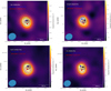 |
Fig. 1 Integrated intensity maps over all velocities for SiO, CH3OH, H2CO, and CS (color coding). Superimposed are the blue (2.09–3.94 km s−1) and red (3.94–7.32 km s−1) emissions for each molecule. Blue and red dots indicate the position of the maximum emissions. The level of each contour (in K km s−1) is indicated in each figure. The color map is the integrated intensity map of each line integrated over all velocities. The black contours show the continuum emission, and the black dot shows its maximum. The levels for the continuum are 5.5 × 10⁻³, 6.0 × 10⁻³, and 6.5 × 10⁻³ mJy. |
7.2 Observation of SiO
We computed an approximate SiO column density in the outflow that is two orders of magnitude lower than that of methanol. Two main questions are raised by the SiO observations. The first question is the processes needed to release silicon in the gas phase, and the second question is the form in which it is released. Gaseous SiO is not observed in quiescent cold cores. In the diffuse interstellar medium, most of the silicon is stored as silicates in the refractory part of the grains. The remaining part in the gas phase, as shown by UV observations, is approximately 1% (abundance of about 1.8 × 10⁻⁶ with respect to total proton density, Jenkins 2009). If Si-bearing molecules are observed in energetic regions (diffuse and translucent clouds, and shocked regions, Turner 1998; Gusdorf et al. 2008), they are not detected in cold dense cores with upper limits on the abundances of about 10−12 for SiO (Ziurys et al. 1989). If the 1% cosmic abundance of silicon were used in astrochemical models, it would produce SiO gas-phase abundances under cold core conditions that would be much higher than the observed upper limit (Mota et al. 2021), even if the reservoir of silicon were SiH4 in the grains, as suggested by Mackay (1996). When the elemental abundance of silicon were decreased to fit the nondetection of SiO in cold cores, the SiO predicted by the models in the ices would then be very low.
When we assume that the observed silicon has been released by a shock, its velocity should be higher than 20 km s−1 (May et al. 2000; Gusdorf et al. 2008), that is, much higher than the SiO velocities that we observed (see also Table 12 of Pineda et al. 2011). For such a high velocity to produce an apparent velocity of 1 km s−1, an angle inclination of 87° would be required (i.e., close to the plan of the sky). The apparent outflow extinction would then be similar to the real length: 1.5″ (half of the emission size of methanol), which represents 423 au at the distance of our source. In this case, its dynamical age would be about 95 yr. If L1451-mm is a protostellar source, this means that it is in a very early stage, maybe the youngest protostar ever observed. SiO is observed in low velocity shocks as well, however, which are not strong enough to destroy the refractory part of the grains (Jiménez-Serra et al. 2010; Nguyen-Lu’o’ng et al. 2013; Sanhueza et al. 2013; Louvet et al. 2016). Nguyen-Lu’o’ng et al. (2013) and Louvet et al. (2016) were able to reproduce their observations in low-velocity shocks with shock models only if a substantial fraction (10%) of the silicon was already in the form of free Si, either in the gas phase or on the grains, or directly in the form of SiO in the grain mantles. SiO was also observed in the low-mass protostar IRAS16293B at low velocities (van der Wiel et al. 2019). Again, the authors suggested that this SiO was produced by some silicon that was still available in the gas phase. In the direction of the low-mass star forming region NGC 1333 IRAS4, Lefloch et al. (1998) detected a very narrow emission of SiO. Comparing the spectral line width of SiO with their narrow H2O emission, Coutens et al. (2013) concluded that both H2O and SiO should come from the photodesorption from the ice mantles in this source or sputtering from grains induced by shocks further decelerated and diluted. In these very dense regions, it is difficult to keep Si in atomic form, however.
Another source of SiO that could be discussed, although more speculatively, is the possible presence of amorphous SiO polymer grains. Krasnokutski et al. (2014) showed experimentally that the polymerization of SiO compounds is barrierless. This process might occur before the formation of the clouds, locking some silicates, and this material might break more easily than silicates in low-velocity shocks and directly produce the observed SiO. Work is still needed to reconcile the nondetection of SiO in cold cores and its observation in these regions, where refractory grains are assumed to be intact.
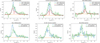 |
Fig. 2 Comparison of the spectral line profiles of the transitions of H2CO, CS, SiO, and CH3OH at three different positions: maximum SiO total integrated intensity position (middle panel), at the blueshifted position ((+0.60″,+0.73″), left panel), and at the redshifted position ((0″, −0.87″), right panel). |
7.3 Nature of the source
With the SiO and class I methanol maser line detections, a shock induced by outflowing gas within ~3″ (i.e., a radius of 430 au, the emission size of the methanol and SiO lines) appears to be established. Shocked regions in FHSCs were predicted by Commerçon et al. (2012) in the case of intermediately and strongly magnetized models. The apparent velocity of the outflow in L1451-mm is closer to the case of the intermediately (their µ = 10 case) magnetized models (outflow with an extent of ~300 au and a velocity ~1 km s−1). The question now is whether a low-velocity outflow like this can release silicon from the grains into the gas phase. With a shock model, Louvet et al. (2016) showed that this is not the case. They needed a shock velocity higher than 7 km s−1 so they had to consider some free silicon in the gas phase to reproduce the SiO observations. Commerçon et al. (2012) suggested that one diagnostic of FHSCs would be that the grains in the outflow would not be destroyed (and then would probably not produce SiO). Hincelin et al. (2016) found that the temperatures in the outflow produced by an FHSC would be lower than ~25 K, except in the very inner (few au) regions. These temperatures would not be high enough to release methanol from the ices, and some potential silicon if any is stored in the ices. As discussed in Sect. 7.1, the observation of the methanol maser cannot indicate the physical conditions as it can be produced under a large range of physical conditions. High concentrations of gas-phase methanol released from the grains are required, however. It is unlikely that the outflows and shocked regions predicted by hydrodynamical models for FHSCs can explain the methanol maser and the SiO lines. We therefore argue that L1451-mm would more probably be a very young low-mass protostar and that the apparent low velocity of the outflow is due to a strong inclination of its axis.
8 Summary and conclusions
We have presented some NOEMA + 30 m data of a few molecules on the L1451-mm source. In particular, we have detected and mapped H2CO, CS, and SiO lines. These three molecules present a double-peak profile that agrees well with an outflow that has been identified by previous publications. We also detected several transitions of methanol. One of these lines appears to be the class I maser line at 146.618 GHz. This specific transition also seems to present a double-peak profile, while some of the methanol transitions have redshifted wings. Non-LTE radiative transfer analysis of the thermal lines of methanol indicates an H2 density of about 3 × 106 cm−3 and a temperature of about 50 K. We detected DCO+, DCN, HDCO, and SO lines, but their emission is rather extended or not on the source. We also detected weak HC3N emission on the source. The SiO and CH3OH maser emission tends to confirm the launch of a compact (expanding to 430 au) and apparently low-velocity (with a characteristic velocity around 1 km s−1) outflow from the central object. Based on current predictions by hydrodynamical models, it is unlikely that an outflow launched by an FHSC could explain our observations of SiO and methanol maser. We therefore argue that L1451-mm more probably is at a very early protostellar stage, launching an outflow with a higher velocity than is observed, and lying nearly in the plan of the sky.
Acknowledgements
The authors acknowledge the CNRS program “Physique et Chimie du Milieu Interstellaire” (PCMI) co-funded by the Centre National d’Études Spatiales (CNES). A.C. is supported by the European Research Council (ERC) under the European Union’s Horizon 2020 research and innovation programme through ERC Starting Grant “Chemtrip” (grant agreement no 949278). The authors thank the IRAM staff, especially Jan Martin Winters, for their help with the observations and calibration of the data. VW thanks Fabrice Herpin from the Laboratoire d’astrophysique de Bordeaux for interesting discussions on masers. The authors are grateful to the anonymous referee for the very helpful suggestions that improved the quality of the paper.
Appendix A Computation of the dust emissivity index
We used our continuum data to compute the dust emissivity index β with equation 2 of Galametz et al. (2019). We obtain β = 0.2. This low index in this wavelength range is usually attributed to millimeter grain sizes (Ysard et al. 2019). Typical values of β in the diffuse interstellar medium are about 1.6 (Planck Collaboration et al. 2014; Juvela et al. 2015). In the starless core TMC-1C (Schnee et al. 2010) and the prestellar core L1544 (Chacón-Tanarro et al. 2019), β was found to be similar to the diffuse interstellar medium or even higher (~2). In class 0 protostars, a gradient in the values of βwas found from interstellar medium-like values in the outer parts of the protostellar envelopes to values lower than one in the inner parts (Galametz et al. 2019). In the class 0 protostar IRAS 2A1, for instance, β was found to be 0.38 at 500 au (see Table 2 of Galametz et al. 2019). Considering the early stage of our object, such low values of β are quite surprising. The dust emissivity index in this source should be investigated with additional observations.
Appendix B Integrated intensity maps
The integrated intensity maps of the detected lines were computed with SpectralCube python package (within the Astropy project; Astropy Collaboration 2013, 2018). A mask was applied on the data to remove signal below the 3 rms limit on each point. The resulting maps are shown in Figs. B.1 to B.4 (color scale) with the continuum emission in gray contours.
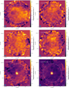 |
Fig. B.1 Integrated intensity maps of detected lines (color scale) with the continuum flux (gray contours at 4.5, 5.5, and 6.5 mJy beam−1). The synthetic beam is indicated by the blue ellipses, and the primary beam is indicated by the large white circle. |
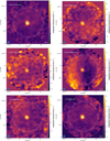 |
Fig. B.2 Integrated intensity maps of detected lines (color scale) with the continuum flux (gray contours at 4.5, 5.5, and 6.5 mJy beam−1). The synthetic beam is indicated by the blue ellipses, and the primary beam is indicated by the large white circle. |
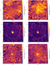 |
Fig. B.3 Integrated intensity maps of detected lines (color scale) with the continuum flux (gray contours at 4.5, 5.5, and 6.5 mJy beam−1). The synthetic beam is indicated by the blue ellipses, and the primary beam is indicated by the large white circle. |
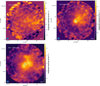 |
Fig. B.4 Integrated intensity maps of detected lines (color scale) with the continuum flux (gray contours at 4.5, 5.5, and 6.5 mJy beam−1). The synthetic beam is indicated by the blue ellipses, and the primary beam is indicated by the large white circle. |
Appendix C Velocity channel maps
This appendix presents the velocity channel maps of the NOEMA+30m data obtained with the GILDAS software (MAPPING). The central plus indicates the position of the continuum maximum. When several lines of a specific molecule have been detected, we only show the brightest line.
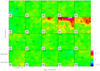 |
Fig. C.1 Channel map for the c-C3H2 line at 150.851 GHz. Color levels are in mJy beam−1. |
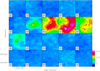 |
Fig. C.2 Channel map for the DCO+ line at 144.077 GHz. Color levels are in Jy beam−1. |
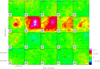 |
Fig. C.3 Channel map for the DCN line at 144.828 GHz. Color levels are in Jy beam−1. |
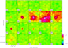 |
Fig. C.4 Channel map for the HDCO line at 128.812 GHz. Color levels are in Jy beam−1. |
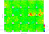 |
Fig. C.5 Channel map for the SO line at 129.138 GHz. Color levels are in Jy beam−1. |
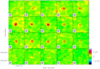 |
Fig. C.6 Channel map for the HC3N line at 145.560 GHz. Color levels are in Jy beam−1. |
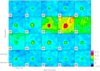 |
Fig. C.7 Channel map for the CS line at 146.969 GHz. Color levels are in Jy beam−1. |
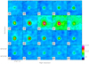 |
Fig. C.8 Channel map for the H2CO line at 145.602 GHz. Color levels are in Jy beam−1. |
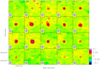 |
Fig. C.9 Channel map for the SiO line at 130.268 GHz. Color levels are in Jy beam−1. |
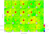 |
Fig. C.10 Channel map for the CH3OH line at 146.618 GHz. Color levels are in Jy beam−1. |
Appendix D Molecular spectra on the source position
This appendix presents all molecular lines detected at the maximum continuum position for the NOEMA+30m data. The vertical dashed lines on the spectra show the local rest velocity of the cloud.
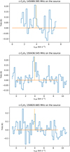 |
Fig. D.1 Spectra of detected lines on the source position. |
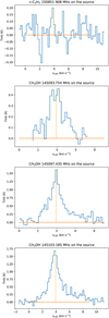 |
Fig. D.2 Spectra of detected lines on the source position. |
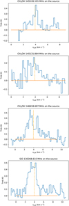 |
Fig. D.3 Spectra of detected lines on the source position. |
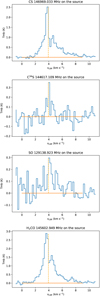 |
Fig. D.4 Spectra of detected lines on the source position. |
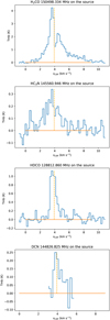 |
Fig. D.5 Spectra of detected lines on the source position. |
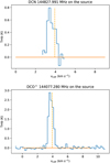 |
Fig. D.6 Spectra of detected lines on the source position. |
Appendix E Molecular column densities in the outflow
To constrain the physical conditions probed by the methanol emission on the source, we performed a χ2 minimization while comparing the observed integrated intensities of the observed lines with a grid of theoretical values. The observed integrated intensities and rms are listed in Table E.1. The grid of theoretical integrated intensities was computed for the six detected lines of methanol using the ndradex6 python package, which in turn uses the non-LTE radiative transfer code RADEX (van der Tak et al. 2007). The collisional coefficients are taken from Rabli & Flower (2010). The computation of the theoretical grid is time consuming, and therefore we first computed a large grid with low resolution, covering H2 densities between 105 and 107 cm−3, temperatures between 20 and 100 K, and CH3OH column densities between 1013 and 1015 cm−2. We then refined around the identified zone with the following grid: 40 values for the temperature in linear space, 20 values for the H2 density between 106 and 107 cm−3 in log space, and 20 values for the CH3OH column density between 5 × 10¹³ and 5 × 1014 cm−3 in log space. We assumed a statistical ratio of 1 of the A and E forms and a line width of 2 km s−1 for all the lines (representative of the mean value of the observed line widths). The results of the χ2 minimization using the six observed lines of CH3OH are shown in Fig. E.1. The best model (with a 3σ confidence level) gives a CH3OH column density of (1.2 ± 0.2) × 1014 cm−2, a temperature of  K, and a H2 density of (3.3 ± 1) × 106 cm−3. Constraints on the methanol column density and the H2 density are rather good, but the constraint on the temperature is weaker. The excitation temperature and optical depth of individual lines as predicted by RADEX for the best model are given in the last two columns of Table E.1. Under these conditions, the 146.618 GHz maser methanol line is predicted with a negative excitation temperature (−5 K) and a peak intensity of 0.3 K (i.e., not very far from our observations). The observed line-integrated intensities are rather well reproduced, except for the two blended lines at 145.126 GHz (left panel of Fig. E.1). We therefore repeated the same χ2 minimization, but only with the four most robust lines (i.e., ignoring the two blended lines). The results are shown in Fig. E.2. The constraints on the physical parameters and the column density are similar, only the temperature is slightly higher. In this case, the best model gives a CH3OH column density of
  cm−2, a temperature of
  K, and a H2 density of (3.8 ± 1) × 106 cm−3.
Using the same procedures, but with the H2 density (3.3 × 106 cm−3) and temperature (50 K) found for the methanol, we computed approximate column densities for CS, H2CO, and SiO in the outflow. For these, we used the intensity integrated over the full velocity range of −0.2 and 10.9 km s−1 (rather than a Gaussian profile fit) because of the more complex line shapes. ndradex was used to compute a grid of 30 values of the column density for each molecule between 1013 and 1014 cm−2 for H2CO, 3 × 10¹² and 3 × 1013 cm−2 for CS, and 3 × 10¹¹ and 3 × 1012 cm−2 for SiO. We detected two lines of H2CO, one for the para form and one for the ortho form. We computed their column densities separately and then summed them. For the line widths, we used the value of an approximate Gaussian fit of each line: 2.6 km s−1 for H2CO, 3.4 km s−1 for CS, and 2.2 km s−1 for SiO. The collisional coefficients are taken from Wiesenfeld & Faure (2013) for H2CO, from Lique et al. (2006) for CS, and from Dayou & Balança (2006) for SiO. The χ2 minimization (with a 3σ confidence level) gives a column density of (8.0 ± 0.3) × 1013 cm−2 for H2CO, (1.2 ± 0.1) × 1013 cm−2 for CS, and (1.6 ± 0.3) × 1012 cm−2 for SiO. Only the NOEMA data were used to focus on the small scales at which CH3OH is seen. For SiO and CH3OH, the line-integrated intensities are the same for NOEMA and NOEMA+30m data. The extended emission on the CS and H2CO lines appears as a narrow intense peak at the rest velocity of the cloud. Removing this component from the lines of the combined data results in column densities similar to what we obtain with the NOEMA data only.
Fitted integrated intensity and rms of the lines used to compute the species column densities. The two last columns are the excitation temperature and optical depth predicted by RADEX (see text).
 |
Fig. E.1 Results of the χ2 minimization using the six observed lines of CH3OH. For each of the three plots on the left, the χ2 is projected over the third axis, which is not shown in the figure. Gray contours represent the 1σ, 2σ, and 3σ confidence intervals. The plot on the right represents the ratio of the observed and modeled integrated intensity for each of the methanol lines and the best model obtained by the χ2 minimization. |
 |
Fig. E.2 Same as Fig. E.1, but for four lines of methanol only (excluding the two 145.126 GHz blended lines). |
References
- Astropy Collaboration (Robitaille, T.P., et al.) 2013, A&A, 558, A33 [NASA ADS] [CrossRef] [EDP Sciences] [Google Scholar]
- Astropy Collaboration (Price-Whelan, A.M., et al.) 2018, AJ, 156, 123 [NASA ADS] [CrossRef] [Google Scholar]
- Bachiller, R. 1996, ARA&A, 34, 111 [NASA ADS] [CrossRef] [Google Scholar]
- Chacón-Tanarro, A., Pineda, J. E., Caselli, P., et al. 2019, A&A, 623, A118 [NASA ADS] [CrossRef] [EDP Sciences] [Google Scholar]
- Commerçon, B., Launhardt, R., Dullemond, C., & Henning, T. 2012, A&A, 545, A98 [NASA ADS] [CrossRef] [EDP Sciences] [Google Scholar]
- Coutens, A., Vastel, C., Cabrit, S., et al. 2013, A&A, 560, A39 [NASA ADS] [CrossRef] [EDP Sciences] [Google Scholar]
- Dayou, F., & Balança, C. 2006, A&A, 459, 297 [NASA ADS] [CrossRef] [EDP Sciences] [Google Scholar]
- Dunham, M. M., Evans, Neal J.I., Bourke, T. L., et al. 2006, ApJ, 651, 945 [NASA ADS] [CrossRef] [Google Scholar]
- Dunham, M. M., Stutz, A. M., Allen, L. E., et al. 2014, in Protostars and Planets VI, eds. H. Beuther, R.S. Klessen, C.P. Dullemond, & T. Henning, 195 [Google Scholar]
- Galametz, M., Maury, A.J., Valdivia, V., et al. 2019, A&A, 632, A5 [NASA ADS] [CrossRef] [EDP Sciences] [Google Scholar]
- Gusdorf, A., Cabrit, S., Flower, D. R., & Pineau Des Forêts, G. 2008, A&A, 482, 809 [NASA ADS] [CrossRef] [EDP Sciences] [Google Scholar]
- Hincelin, U., Commerçon, B., Wakelam, V., et al. 2016, ApJ, 822, 12 [NASA ADS] [CrossRef] [Google Scholar]
- Jenkins, E. B. 2009, ApJ, 700, 1299 [Google Scholar]
- Jiménez-Serra, I., Caselli, P., Tan, J. C., et al. 2010, MNRAS, 406, 187 [Google Scholar]
- Juvela, M., Demyk, K., Doi, Y., et al. 2015, A&A, 584, A94 [NASA ADS] [CrossRef] [EDP Sciences] [Google Scholar]
- Kalenskii, S. V., Johansson, L. E. B., Bergman, P., et al. 2010, MNRAS, 405, 613 [NASA ADS] [Google Scholar]
- Krasnokutski, S. A., Rouillé, G., Jäger, C., et al. 2014, ApJ, 782, 15 [NASA ADS] [CrossRef] [Google Scholar]
- Larson, R. B. 1969, MNRAS, 145, 271 [Google Scholar]
- Lefloch, B., Castets, A., Cernicharo, J., & Loinard, L. 1998, ApJ, 504, L109 [NASA ADS] [CrossRef] [Google Scholar]
- Leurini, S., Menten, K. M., & Walmsley, C. M. 2016, A&A, 592, A31 [NASA ADS] [CrossRef] [EDP Sciences] [Google Scholar]
- Lique, F., Spielfiedel, A., & Cernicharo, J. 2006, A&A, 451, 1125 [NASA ADS] [CrossRef] [EDP Sciences] [Google Scholar]
- Louvet, F., Motte, F., Gusdorf, A., et al. 2016, A&A, 595, A122 [NASA ADS] [CrossRef] [EDP Sciences] [Google Scholar]
- Mackay, D. D. S. 1996, MNRAS, 278, 62 [NASA ADS] [CrossRef] [Google Scholar]
- Maureira, M. J., Arce, H. G., Dunham, M. M., et al. 2017, ApJ, 838, 60 [NASA ADS] [CrossRef] [Google Scholar]
- Maureira, M. J., Arce, H. G., Dunham, M. M., et al. 2020, MNRAS, 499, 4394 [NASA ADS] [CrossRef] [Google Scholar]
- May, P. W., Pineau des Forêts, G., Flower, D.R., et al. 2000, MNRAS, 318, 809 [NASA ADS] [CrossRef] [Google Scholar]
- Menten, K. M. 1991, in Atoms, Ions and Molecules: New Results in Spectral Line Astrophysics, eds. A.D. Haschick & P.T.P. Ho, Astronomical Society of the Pacific Conference Series, 16, 119 [NASA ADS] [Google Scholar]
- Menten, K. M. 1997, IAU Symp., 178, 163 [NASA ADS] [Google Scholar]
- Mota, V. C., Varandas, A. J. C., Mendoza, E., Wakelam, V., & Galvão, B. R. L. 2021, ApJ, 920, 37 [NASA ADS] [CrossRef] [Google Scholar]
- Müller, H. S. P., Menten, K. M., & Mäder, H. 2004, A&A, 428, 1019 [NASA ADS] [CrossRef] [EDP Sciences] [Google Scholar]
- Müller, H. S. P., Schlöder, F., Stutzki, J., & Winnewisser, G. 2005, J. Mol. Struct., 742, 215 [Google Scholar]
- Nesterenok, A. V. 2021, J. Phys.: Conf. S., 2103, 012012 [NASA ADS] [CrossRef] [Google Scholar]
- Nguyen-Lu’o’ng, Q., Motte, F., Carlhoff, P., et al. 2013, ApJ, 775, 88 [CrossRef] [Google Scholar]
- Pety, J. 2005, in SF2A-2005: Semaine de l’Astrophysique Française, eds. F. Casoli, T. Contini, J.M. Hameury, & L. Pagani, 721 [Google Scholar]
- Pezzuto, S., Elia, D., Schisano, E., et al. 2012, A&A, 547, A54 [NASA ADS] [CrossRef] [EDP Sciences] [Google Scholar]
- Pezzuto, S., Benedettini, M., Di Francesco, J., et al. 2021, A&A, 645, A55 [EDP Sciences] [Google Scholar]
- Pickett, H. M., Poynter, R. L., Cohen, E. A., et al. 1998, J. Quant. Spec. Radiat. Transf., 60, 883 [Google Scholar]
- Pineda, J. E., Arce, H. G., Schnee, S., et al. 2011, ApJ, 743, 201 [NASA ADS] [CrossRef] [Google Scholar]
- Pineda, J. E., Zhao, B., Schmiedeke, A., et al. 2019, ApJ, 882, 103 [NASA ADS] [CrossRef] [Google Scholar]
- Planck Collaboration XI. 2014, A&A, 571, A11 [NASA ADS] [CrossRef] [EDP Sciences] [Google Scholar]
- Rabli, D., & Flower, D. R. 2010, MNRAS, 406, 95 [Google Scholar]
- Robitaille, T., & Bressert, E. 2012, APLpy: Astronomical Plotting Library in Python, Astrophysics Source Code Library, [record ascl:1208.017] [Google Scholar]
- Sanhueza, P., Jackson, J. M., Foster, J. B., et al. 2013, ApJ, 773, 123 [NASA ADS] [CrossRef] [Google Scholar]
- Schnee, S., Enoch, M., Noriega-Crespo, A., et al. 2010, ApJ, 708, 127 [NASA ADS] [CrossRef] [Google Scholar]
- Stephens, I. W., Bourke, T. L., Dunham, M. M., et al. 2019, ApJS, 245, 21 [CrossRef] [Google Scholar]
- Tomida, K., Tomisaka, K., Matsumoto, T., et al. 2010, ApJ, 714, L58 [NASA ADS] [CrossRef] [Google Scholar]
- Turner, B. E. 1998, ApJ, 495, 804 [NASA ADS] [CrossRef] [Google Scholar]
- van der Tak, F.F.S., Black, J. H., Schöier, F. L., Jansen, D. J., & van Dishoeck, E. F. 2007, A&A, 468, 627 [NASA ADS] [CrossRef] [EDP Sciences] [Google Scholar]
- van der Wiel, M. H. D., Jacobsen, S. K., Jørgensen, J. K., et al. 2019, A&A, 626, A93 [NASA ADS] [CrossRef] [EDP Sciences] [Google Scholar]
- Vorobyov, E. I., Elbakyan, V., Dunham, M. M., & Guedel, M. 2017, A&A, 600, A36 [NASA ADS] [CrossRef] [EDP Sciences] [Google Scholar]
- Wiesenfeld, L., & Faure, A. 2013, MNRAS, 432, 2573 [NASA ADS] [CrossRef] [Google Scholar]
- Young, A. K., Bate, M. R., Harries, T. J., & Acreman, D. M. 2019, MNRAS, 487, 2853 [NASA ADS] [CrossRef] [Google Scholar]
- Ysard, N., Koehler, M., Jimenez-Serra, I., Jones, A. P., & Verstraete, L. 2019, A&A, 631, A88 [NASA ADS] [CrossRef] [EDP Sciences] [Google Scholar]
- Ziurys, L. M., Friberg, P., & Irvine, W. M. 1989, ApJ, 343, 201 [NASA ADS] [CrossRef] [Google Scholar]
- Zucker, C., Schlafly, E. F., Speagle, J. S., et al. 2018, ApJ, 869, 83 [NASA ADS] [CrossRef] [Google Scholar]
The effective radius was recomputed with respect to the value given in the paper to take the change in the distance of the source into account.
All Tables
Fitted integrated intensity and rms of the lines used to compute the species column densities. The two last columns are the excitation temperature and optical depth predicted by RADEX (see text).
All Figures
|
Fig. 1 Integrated intensity maps over all velocities for SiO, CH3OH, H2CO, and CS (color coding). Superimposed are the blue (2.09–3.94 km s−1) and red (3.94–7.32 km s−1) emissions for each molecule. Blue and red dots indicate the position of the maximum emissions. The level of each contour (in K km s−1) is indicated in each figure. The color map is the integrated intensity map of each line integrated over all velocities. The black contours show the continuum emission, and the black dot shows its maximum. The levels for the continuum are 5.5 × 10⁻³, 6.0 × 10⁻³, and 6.5 × 10⁻³ mJy. |
| In the text | |
|
Fig. 2 Comparison of the spectral line profiles of the transitions of H2CO, CS, SiO, and CH3OH at three different positions: maximum SiO total integrated intensity position (middle panel), at the blueshifted position ((+0.60″,+0.73″), left panel), and at the redshifted position ((0″, −0.87″), right panel). |
| In the text | |
|
Fig. B.1 Integrated intensity maps of detected lines (color scale) with the continuum flux (gray contours at 4.5, 5.5, and 6.5 mJy beam−1). The synthetic beam is indicated by the blue ellipses, and the primary beam is indicated by the large white circle. |
| In the text | |
|
Fig. B.2 Integrated intensity maps of detected lines (color scale) with the continuum flux (gray contours at 4.5, 5.5, and 6.5 mJy beam−1). The synthetic beam is indicated by the blue ellipses, and the primary beam is indicated by the large white circle. |
| In the text | |
|
Fig. B.3 Integrated intensity maps of detected lines (color scale) with the continuum flux (gray contours at 4.5, 5.5, and 6.5 mJy beam−1). The synthetic beam is indicated by the blue ellipses, and the primary beam is indicated by the large white circle. |
| In the text | |
|
Fig. B.4 Integrated intensity maps of detected lines (color scale) with the continuum flux (gray contours at 4.5, 5.5, and 6.5 mJy beam−1). The synthetic beam is indicated by the blue ellipses, and the primary beam is indicated by the large white circle. |
| In the text | |
|
Fig. C.1 Channel map for the c-C3H2 line at 150.851 GHz. Color levels are in mJy beam−1. |
| In the text | |
|
Fig. C.2 Channel map for the DCO+ line at 144.077 GHz. Color levels are in Jy beam−1. |
| In the text | |
|
Fig. C.3 Channel map for the DCN line at 144.828 GHz. Color levels are in Jy beam−1. |
| In the text | |
|
Fig. C.4 Channel map for the HDCO line at 128.812 GHz. Color levels are in Jy beam−1. |
| In the text | |
|
Fig. C.5 Channel map for the SO line at 129.138 GHz. Color levels are in Jy beam−1. |
| In the text | |
|
Fig. C.6 Channel map for the HC3N line at 145.560 GHz. Color levels are in Jy beam−1. |
| In the text | |
|
Fig. C.7 Channel map for the CS line at 146.969 GHz. Color levels are in Jy beam−1. |
| In the text | |
|
Fig. C.8 Channel map for the H2CO line at 145.602 GHz. Color levels are in Jy beam−1. |
| In the text | |
|
Fig. C.9 Channel map for the SiO line at 130.268 GHz. Color levels are in Jy beam−1. |
| In the text | |
|
Fig. C.10 Channel map for the CH3OH line at 146.618 GHz. Color levels are in Jy beam−1. |
| In the text | |
|
Fig. D.1 Spectra of detected lines on the source position. |
| In the text | |
|
Fig. D.2 Spectra of detected lines on the source position. |
| In the text | |
|
Fig. D.3 Spectra of detected lines on the source position. |
| In the text | |
|
Fig. D.4 Spectra of detected lines on the source position. |
| In the text | |
|
Fig. D.5 Spectra of detected lines on the source position. |
| In the text | |
|
Fig. D.6 Spectra of detected lines on the source position. |
| In the text | |
|
Fig. E.1 Results of the χ2 minimization using the six observed lines of CH3OH. For each of the three plots on the left, the χ2 is projected over the third axis, which is not shown in the figure. Gray contours represent the 1σ, 2σ, and 3σ confidence intervals. The plot on the right represents the ratio of the observed and modeled integrated intensity for each of the methanol lines and the best model obtained by the χ2 minimization. |
| In the text | |
|
Fig. E.2 Same as Fig. E.1, but for four lines of methanol only (excluding the two 145.126 GHz blended lines). |
| In the text | |
Current usage metrics show cumulative count of Article Views (full-text article views including HTML views, PDF and ePub downloads, according to the available data) and Abstracts Views on Vision4Press platform.
Data correspond to usage on the plateform after 2015. The current usage metrics is available 48-96 hours after online publication and is updated daily on week days.
Initial download of the metrics may take a while.