| Issue |
A&A
Volume 689, September 2024
|
|
|---|---|---|
| Article Number | A76 | |
| Number of page(s) | 25 | |
| Section | Interstellar and circumstellar matter | |
| DOI | https://doi.org/10.1051/0004-6361/202349136 | |
| Published online | 03 September 2024 | |
Revisiting the massive star-forming complex RCW 122: New millimeter and submillimeter study
1
Instituto de Astrofísica de La Plata (UNLP – CONICET),
La Plata,
Argentina
e-mail: This email address is being protected from spambots. You need JavaScript enabled to view it.
2
Departamento de Astronomía, Universidad de Chile,
Casilla 36,
Santiago de Chile,
Chile
3
Instituto de Astronomía y Física del Espacio (UBA, CONICET),
CC 67, Suc. 28,
1428
Buenos Aires,
Argentina
4
Dept. Ciencias Integradas, Facultad de Ciencias Experimentales, Centro de Estudios Avanzados en Física, Matemática y Computación, Unidad Asociada GIFMAN, CSIC-UHU, Universidad de Huelva,
Spain
5
Instituto Universitario Carlos I de Física teórica y Computacional, Universidad de Granada,
Spain
6
Facultad de Ciencias Astronómicas y Geofísicas, Universidad Nacional de La Plata,
Paseo del Bosque s/n,
1900
La Plata,
Argentina
Received:
30
December
2023
Accepted:
26
June
2024
Abstract
In this paper, we present a new multifrequency study of the giant star-forming complex RCW 122. We used molecular data obtained with the ASTE 10 m and the APEX 12 m telescopes, along with infrared observations spanning from 3.6 µm to 870 µm, obtained from available databases. We also incorporated a range of public datasets, including the radio continuum at 3 GHz, narrowband Ha images, and deep JHK photometry. Our analysis focuses mostly on cataloged ATLASGAL sources, showcasing a spectrum of evolutionary stages from infrared dark cloud (IRDC)/high-mass protostellar object (HMPO) to ultra-compact HII region (UCHII), as inferred from preliminary inspections of the public dataset. Based on ASTE HCO+(4−3) and CO(3−2) data, we identified five molecular clumps, designated A, B, C, D, and E, as molecular counterparts of the ATLASGAL sources. These clumps have radial velocities ranging from ~−15 km s−1 to −10 km s−1, confirming their association with RCW 122. In addition, we report the detection of 20 transitions from 11 distinct molecules in the APEX spectra in the frequency ranges from 258.38 GHz to 262.38 GHz, 228.538 GHz to 232.538 GHz, and 218.3 GHz to 222.3 GHz, unveiling a diverse chemical complexity among the clumps. Utilizing CO(2−1) and C18O(2−1) data taken from the observations with the APEX telescope, we estimated the total LTE molecular mass, ranging from 200 M⊙ (clump A) to 4400 M⊙ (clump B). Our mid- to far-infrared (MIR-FIR) flux density analysis yielded minimum dust temperatures of 23.7 K (clump A) to maximum temperatures of 33.9 K (clump B), indicating varying degrees of internal heating among the clumps. The bolometric luminosities span 1.7×10³ L⊙ (clump A) to 2.4×10⁵ L⊙ (clump B), while the total (dust+gas) mass ranges from 350 M⊙ (clump A) to 3800 M⊙ (clump B). Our analysis of the molecular line richness, L/M ratios, and CH3CCH and dust temperatures reveals an evolutionary sequence of A/E→C→D/B, consistent with preliminary inferences of the ATLASGAL sources. In this context, clumps A and E exhibit early stages of collapse, with clump A likely in an early HMPO phase, which is supported by identifying a candidate molecular outflow. Clump E appears to be in an intermediate stage between IRDC and HMPO. Clumps D and B show evidence of being in the UCHII phase, with clump B likely more advanced. Clump C likely represents an intermediate stage between HMPO and HMC. Our findings suggest clump B is undergoing ionization and heating by multiple stellar and protostellar members of the stellar cluster DBS 119. Meanwhile, other cluster members may be responsible for ionizing other regions of RCW 122 that have evolved into fully developed HII regions, beyond the molecular dissociation stage.
Key words: astrochemistry / stars: formation / HII regions / ISM: molecules / submillimeter: ISM / ISM: individual objects: RCW 122
Member of the Carrera del Investigador Científico of CONICET, Argentina.
© The Authors 2024
 Open Access article, published by EDP Sciences, under the terms of the Creative Commons Attribution License (https://creativecommons.org/licenses/by/4.0), which permits unrestricted use, distribution, and reproduction in any medium, provided the original work is properly cited.
This article is published in open access under the Subscribe to Open model. This email address is being protected from spambots. You need JavaScript enabled to view it. to support open access publication.
1 Introduction
Massive stars play an essential role in the evolution of the interstellar medium (ISM) of galaxies. They influence the chemical and dynamical evolution of galaxies and affect their surrounding environments through their energetic feedback (ionizing radiation, stellar winds, and, eventually, supernova explosions). Therefore, the formation of massive stars is a crucial topic in astrophysics. Still, the process remains poorly understood because of their large distances and short lifetime, compared with their low-mass counterparts. Further, high-mass stars are born in clusters or multiple complex systems, spending most of their early stages embedded in their dense parental molecular surroundings, where the high-density gas and dust prevent visible light from escaping.
From an observational point of view, the formation of massive stars could be divided into four different stages (see Zinnecker & Yorke 2007): (1) cold massive starless clouds, also known as infrared dark clouds (IRDCs): they can be identified due to their high extinctions at near-infrared (NIR) and mid-infrared (MIR) wavelengths. They can be detected mostly in the (sub-)millimeter and/or far-infrared (FIR) range (Egan et al. 1998; Rathborne et al. 2006). They have typical sizes of 1–10 pc, volume densities of ≳ 104 cm−3, and temperatures T ≲ 20 K; (2) hot molecular cores (HMCs): they are formed as the central pro-tostar heats the envelope (T ≥ 100 K) and molecules residing in the icy mantles of dust grains evaporate into the gas-phase; that makes HMCs strong emitters of a wealth of complex molecules, even organic (e.g., HC3N, CH3OH, CH3CN, CH3CCH, and CH3OCHO) in the millimeter and submillimeter range (van Dishoeck & Blake 1998; Belloche et al. 2013; Beltrán et al. 2018); (3) ultra-compact HII regions (UCHII): Formed as pro-tostellar radiation expands and further dissipates and ionizes the surrounding molecular envelope. These regions are detectable in the radio continuum and the millimeter ranges (Garay & Lizano 1999; Hoare et al. 2007; Sánchez-Monge et al. 2013); and (4) classical HII regions powered by O-B stars: detected primarily on radio continuum and optical ranges. According to this scheme, stage (1) could be next followed by the intermediate so-called high-mass protostellar object (HMPO) stage (Williams et al. 2004; Motte et al. 2007; Beuther et al. 2010), which is detected mainly at millimeter and MIR wavelengths due to the internal heating of a central accreting protostar. By stage (2), the ionizing radiation of the protostar in the central region of the HMC can give rise to a hyper-compact HII region (HCHII). Class II 6.7-GHz CH3OH maser emission can be observed in stages (1) and (2) (Walsh et al. 2001), while H2O maser emission can be detected in stages (1) to (3). Molecular outflows can be detected from the HMPO to the UCHII stage (Kurtz et al. 2000; Beuther et al. 2002, 2007).
Detailed observations of massive protostellar objects within their parental molecular nurseries are essential for empirically constraining existing theoretical models and improving our understanding of the physical processes driving the formation and evolution of massive stars. To this end, millimeter and submillimeter/infrared observations are crucial since they can penetrate dense regions and probe the physical and chemical properties of the molecular gas and dust where the star formation is (or will be) taking place (e.g., Bronfman et al. 2008; Merello et al. 2013; Duronea et al. 2017, 2019; Mendoza et al. 2018; Santos et al. 2022).
The star-forming complex RCW 122 is a giant HII region situated in the fourth quadrant of the Galactic plane. The whole complex is associated with a large molecular cloud of 2.2 × 10⁵ M⊙ (see Arnal et al. 2008). The region has three main sources identified by McBreen et al. (1985) as RCW 122A, RCW 122B, and RCW 122C. In particular, the ensemble RCW122AB (from here onwards RCW122) is centered at RA, Dec (J2000)=(17:20:02,−38:57:45) and it seems to be associated with the embedded cluster DBS 119 (Dutra et al. 2003; Morales et al. 2013). The finding chart depicting these components and their close surroundings is presented in Fig. 1. In the right panel of the figure, we present an Hα emission image that reveals various features such as ionization fronts, bright-rimmed clouds, and high extinction regions. In the left panel of the figure, we display the Spitɀer/IRAC emission at 8.0, 4.5, and 3.6 µm overlaid onto the 870 µm continuum emission obtained from the ATLASGAL database. This reveals a rich diversity of complex structures like filaments, cores, fingers, and bow shocks.
Evidence of massive star formation in RCW 122 was reported by Sollins & Megeath (2004), who detected two spots of HC3N emission (a typical HMC molecule) at the positions RA, Dec (B1950) = (17:16:39.6, −38:54:16) and RA, Dec (B 1950) = (17:16:31.9, −38:55:21), referred to in that work as RCW 122(NE) and RCW 122(SW), respectively. These spots are spatially coincident with bright Spitɀer/IRAC regions and with two 870 µm emission clumps, classified in the ATLASGAL catalog of Contreras et al. (2013) as AGAL348.726-01.039 and AGAL348.698-01.027, respectively (see left panel of Fig. 1). Furthermore, RCW 122(NE) is a strong maser emitter of H2 O (Braz & Epchtein 1983; Forster & Caswell 1989), OH (Scalise & Alcina Braz 1980; Forster & Caswell 1989), and CH3 OH (Chen et al. 2011; Yang et al. 2017). Besides, three other conspicuous 870 µm clumps were cataloged in the region, identified by Contreras et al. (2013) as AGAL348.701-01.042, AGAL348.754-01.069, and AGAL348.649-01.069, which were also indicated in the left panel of Fig. 1. The existence of these clumps indicates the presence of high-density gas and dust. Another spot of H2O and CH3OH maser emission was identified in the direction of AGAL348.701-01.042.
The star formation activity in RCW 122 may be revealed by the detection of the so-called extended green objects (EGOs), which are sources identified by their extended emission in the Spitɀer/IRAC 4.5 µm band, often associated with shocked molecular hydrogen from protostellar outflows (Cyganowski et al. 2008). Two EGOs, identified by Cyganowski et al. (2008) as “possible” MYSO outflow candidates and designated as G348.72–1.04 and G348.73-1.04, were found projected at the center of AGAL348.726-01.039 (see left panel of Fig. 1).
The presence of ionized gas in RCW 122 is unveiled by the 3 GHz radio continuum and Hα emissions (presented in the right panel of Fig. 1). Unlike the Hα emission, which appears diffuse and scattered throughout the complex, the radio continuum emission at 3 GHz is compact and concentrated toward AGAL348.726-01.039 and AGAL348.698-01.027. This apparent anticorrelation may have an explanation. Specifically, the absence of Hα emission toward the center of the AGAL sources could be attributed to high extinction in the optical band, while the lack of extended emission at 3 GHz inside and outside the center of the sources may result from the absence of short spac-ings in the VLASS radio observations (see Sect. 2.2). However, despite the potential loss of extended structures in the radio continuum, the detection of ionized gas toward the 870 µm emission peak of both AGAL348.726-01.039 and AGAL348.698-01.027 suggests the presence of embedded young HII regions. Moreover, the detection of HMC molecules in the vicinity of these sources suggests that they are still in an early stage, probably UCHII.
Hence, the molecular complex associated with RCW 122 is an excellent candidate for star formation studies of giant molecular clouds. While the analysis by Arnal et al. (2008) offered valuable insights into the general properties of the molecular gas and dust in RCW 122, the spatial resolution of their NANTEN CO(1-0) observations did not permit a detailed analysis in specific locations where the star formation is occurring. Consequently, a comprehensive study of RCW 122 employing higher spatial resolution millimeter and submillime-ter observations is required. This would enable the correlation of large-scale structures with small-scale structures (clumps and/or cores) and provide a more thorough understanding of the conditions of the molecular gas and dust in the region. Specifically, a detailed analysis should be focused on the sources AGAL348.726-01.039, AGAL348.701-01.042, AGAL348.698-01.027, AGAL348.754-01.069, and AGAL348.649-01.069 (hereafter, the “AGAL sources”). Upon confirmation on whether the AGAL sources are part of the same molecular complex (henceforth originating from the same molecular cloud with similar initial conditions) a quantitative analysis and comparison of their physical and chemical properties would provide valuable insights. To that end, by combining the observational information summarized thus far, in Table 1 we put forward a tentative evolutionary classification of the sources. The sequence goes from top to bottom. Although this classification is coarse, comparing physical and chemical properties among the sources will be instructive. It is important to note that due to the similarities in the observational characteristics of AGAL348.754-01.069 and AGAL348.754-01.069, it is challenging to establish an evolutionary distinction between the sources. Therefore, the proposed grading is arbitrary.
The main scope of this work is to improve the analysis of the molecular and dust components associated with the star-forming complex/HII region RCW 122, focusing special attention on the AGAL sources. We aim to identify and study their molecular counterparts by determining their main physical and chemical properties. We also aim to establish a possible evolutionary sequence of the sources, relying on both, the classification scheme proposed before and the physical and chemical properties further derived from the millimeter and submillime-ter data. We use molecular data obtained with the Atacama Pathfinder Experiment (APEX) 12 m and Atacama Submillime-ter Telescope (ASTE) 10 m. The excellent spatial resolution and sensitivity of SHiFI APEX-1 (APEX) and DASH345 (ASTE) instruments (almost 5 times higher than NANTEN) make them well suitable to improve the analysis of the molecular gas and to complement available MIR and FIR data. To perform a complete study of the stellar formation activity in the complex, we also aim to detect and identify the stellar population of the embedded cluster DBS 119, likely to be associated with RCW 122. We additionally look for new young stellar objects (YSOs) candidates to clarify the connection between them and their parental molecular nurseries.
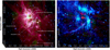 |
Fig. 1 Studied region of RCW 122. Left panel: composite images in red, green, and blue colors show emission at 8.0, 4.5, and 3.6 µm (Spitɀer/IRAC), respectively. Green contours represent the 870 µm dust continuum emission from the ATLASGAL survey, with levels of 0.6 (~8 r ms), 1.2, 2.3, 4.8, 8, and 15 Jy beam−1. White arrows and labels indicate the position of ATLASGAL clumps identified by Contreras et al. (2013) and the HC3N spots reported by Sollins & Megeath (2004) (see text). Right panel: SuperCosmos Hα emission image (blue color) superimposed on the VLASS radio continuum image at 3 GHz (red color). As presented in the left panel, the green contours represent the 870 µm emission. |
Overview of observational features and proposed evolutionary stages for the AGAL sources.
2 Observations
2.1 Molecular observations
2.1.1 APEX data
The observations were obtained in June 2014 using the APEX 12 m telescope (Güsten et al. 2006) located at Llano de Chajnan-tor (Chile). As the front end for the observations, we used the APEX-1 receiver of the Swedish Heterodyne Facility Instrument (SHeFI; Vassilev et al. 2008). The back end for all observations was the eXtended bandwidth Fast Fourier Transform Spec-trometer2 (XFFTS2) with a 2.5 GHz bandwidth divided into 32768 channels, providing a velocity resolution of ~0.1 km s−1. Two 2.5 GHz XFFTS2 boards (X201 and X202) combined, with 500 MHz overlap, provide a 4 GHz-wide spectrometer. The observed transitions and basic observational parameters are summarized in Table 2. Calibration was performed using the chopper-wheel technique, and the output intensity scale given by the system is TA, representing the antenna temperature corrected for atmospheric attenuation. The observed intensities were converted to the main-beam brightness temperature scale by Tmb = TA/ηmb, where ηmb is the main beam efficiency. For the SHeFI/APEX-1 receiver we adopted ηmb = 0.75.
Observations were made using the on-the-fly (OTF) mode with two orthogonal scan directions along RA and Dec(J2000) centered on RA, Dec (J2000)=(17:20:04, −38:57:23). To observe the lines CO(2−1), 13CO(2−1), C18O(2−1), we mapped a region of ~10′ × 10′ in size, tunning the receiver at 230.538 GHz for CO(2−1) (frequency range from 228.538 GHz to 232.538 GHz), and at 220.3 GHz for 13CO(2−1) and C18O(2−1) (frequency range from 218.3 GHz to 222.3 GHz), while to observe the central densest region of the nebula, to observe the H13CO+(3−2) line, we mapped a region of 5′×5′ in size, tuning the receiver at 260.380 GHz (frequency range from 258.38 GHz to 262.38 GHz). The spectra were reduced using the CLASS90 program of the IRAM GILDAS package1 (Pety 2005). To identify the lines we utilized the CDMS2 (Müller et al. 2005) and JPL3 (Pickett et al. 1998) spectroscopy databases, which were interactively loaded on the survey using the WEEDS extension of CLASS (Maret et al. 2011). The spectral analysis was performed using the CASSIS software4 (Vastel et al. 2015).
2.1.2 ASTE data
The observations with the ASTE 10 m telescope (Ezawa et al. 2004, 2008) were carried out in August 2014. We used DASH345, a two-sideband single-polarization heterodyne receiver, tunable in LO frequency range from 327 GHz to 370 GHz at the observable frequency range from 321 GHz to 376 GHz (ηmb = 0.65). The XF digital spectrometer was set to a bandwidth and spectral resolution of 128 MHz (~110 km s−1) and 125 KHz (~0.11 km s−1), respectively. We aimed to observe simultaneously the pair CO(3−2)/HCO+ (4−3) over an area of 16′×16′ in size. Observations were made using the on-the-fly (OTF) mode with two orthogonal scan directions along the center on RA, Dec (J2000)=(17:19:47, −38:59:34). The observed transitions and basic observational parameters are summarized in Table 2. The spectra were reduced with NOSTAR5 using the standard procedure6.
Observational parameters of the molecular transitions observed with APEX and ASTE.
2.2 Archival data
The observations detailed in the previous sections were complemented by the following publicly available data:
Image of ATLASGAL at 870 µm (345 GHz) (Schuller et al. 2009). The image has a root mean square (rms) noise of ~0.05– 0.07 Jy beam−1 and a beam size of ~ 19″.2.
Images from the Herschel7 Infrared GALactic (Hi-GAL) plane survey key program (Molinari et al. 2010). We used images from the Photometric Array Camera and Spectrometer (PACS) survey at 70 and 160 µm, with an FWHM of 5″.5 and 11″, respectively. Additionally, we used images from the Spectral and Photometric Imaging Receiver (SPIRE) at 250, 350, and 500 µm each with an FHWM of 17″.6, 23″.9, and 35″.2, respectively.
Images at 3.6, 4.5, and 8.0 µm from the Galactic Legacy Infrared Mid-Plane Survey Extraordinaire (Spitɀer/GLIMPSE, Benjamin et al. 2003), retrieved from the Spitɀer Science Center8. The images have a spatial resolution of ~2″.
Images at 8.3, 12.1, 14.7, and 21.3 µm retrieved from the Midcourse Space Experiment (MSX)9 (Price et al. 2001). The images have a spatial resolution of 18″.3.
Image of narrow band Hα data: Retrieved from the SuperCOSMOS Hα Survey10 (SHS). The image has a spatial resolution of ~1″ (Parker et al. 2005).
Image of radio continuum at 3 GHz extracted from VLA Sky Survey (VLASS; Lacy et al. 2020). The angular resolution and sensitivity are about 2″.5 and 100 µJy beam−1, respectively. The image is primary beam corrected.
The deep JHK photometric catalog based on the “Vista Variables in the Via Láctea” (VVV) survey (Minniti et al. 2010; Saito et al. 2012; Zhang & Kainulainen 2019). It was complemented with information from the “Two Micron All-Sky Survey” (2MASS) catalog (Skrutskie et al. 2006) to obtain the photometry of saturated stars in the VVV survey.
3 Results and analysis
3.1 Molecular emission
3.1.1 Low- and medium-density molecular gas and comparison with other wavelengths
To thoroughly examine the molecular gas component associated with RCW 122, we focused on the molecular emission observed within the velocity range from ~−23 to −8 km s−1, as identified by Arnal et al. (2008) since, as the authors demonstrated, this component is unequivocally associated with the star-forming complex. To reveal the spatial distribution of low- and medium-density molecular gas, we analyzed the carbon monoxide emissions in the transitions CO(3−2), CO(2−1), 13CO(2−1), and C18O(2−1). The thick/moderately thick lines CO(3−2), CO(2−1), and 13CO(2−1) are good tracers of the outer parts of clouds and clumpy structures, while the optically thin C18O(2−1) line is expected to trace the emission of the inner regions.
In Fig. 2, we present the emission of the CO(3−2), CO(2−1), 13CO(2−1), and C18O(2−1) lines within their total velocity intervals. As the figure illustrates, their emission is intense and extends widely across the field of view, encompassing areas well beyond the coverage of our APEX and ASTE observations. Further, the first contour levels shown in Fig. 2 are tens of times the rms noise, even for the optically thin C18O(2−1) line. However, it is noteworthy that the carbon monoxide emission closely follows the faintest 870 µm and 8 µm emission in the most extended regions of the complex (see the left panel of Fig 1). The 8 µm emission can be a tracer of photodissociated regions (PDRs) because it originates from PAH emission features illuminated by FUV radiation. This indicates the presence of PDRs formed over the molecular gas due to the influence of stellar radiation. The presence of several bright and extended spots and rims of Hα emission which, as mentioned in Sect. 1, are spatially dispersed along the complex indicating the existence of HII regions, aligns with this scenario. Overall, this suggests the presence of evolved massive star(s) within the molecular complex, contributing to the formation and maintenance of these PDRs and HII regions.
From Fig. 2, it can be noted that the most intense carbon monoxide emission originates from the central region of the nebula, particularly in the vicinity of sources AGAL348.726-01.039, AGAL348.701-01.042, and AGAL348.698-01.027 which suggests that these sources represent the densest region of the molecular complex. As previously noted in Sect. 1, the detection of radio continuum emission at 3 GHz indicates the presence of ionized gas toward the 870 µm peak emission of AGAL348.726-01.039 and AGAL348.698-01.027, which are also coincident with the emission peak of C18O(2−1). For the single radio source associated with AGAL348.698-01.027, we estimated an integrated flux density at 3 GHz of ~0.9 Jy. Therefore, using Eq. (A.2.5) of Panagia & Walmsley (1978), considering a distance of 3.38 kpc (see Sect. 3.1.2), an angular radius of about 0.05′, and assuming an electron temperature of 104 K, we derived an electron density of about 1.5 × 104 cm−3. This likely represents a lower limit density given that the radio continuum emission is in the optically thick regime at this frequency. Hence, the linear size (~0.1 pc) and the electron density of this compact radio source agree with typical values reported in UCHII regions (Murphy et al. 2010). Assuming that a single young star is responsible for ionizing the gas, we can speculate about its spectral type based on the estimated radio flux density. We derived the number of photons needed to sustain the ioniza-tion in the source from  (see Chaisson 1976), which yielded to Nuυ = (1.1 ± 0.3) × 1048 ph s−1. Based on Martins et al. (2005), we conclude that the spectral type of the exciting star should be earlier than O9V.
On the other hand, the 3 GHz radio emission associated with AGAL348.726-01.039 displays a more extended and patchy spatial distribution. This characteristic suggests a more advanced evolutionary stage for this HII region than that associated with AGAL348.698-01.027. However, whether the ionization is driven by a high-mass star from a previous stellar generation or by obscured nascent stellar sources remains unclear. This aspect will be further investigated in Sect. 3.3. Unfortunately, due to the lack of short spacing in the used VLASS image, we were unable to extract a reliable total flux density for this region.
Therefore, while the Hα and 3 GHz emissions denote the presence of ionized gas in the region, their origins likely differ. The Hα emission probably arises from the ionization of less dense external layers of the parental molecular cloud traced by the weaker optically thick CO emission. This could be attributed to a previous generation of high-mass stars formed in the region. On the other hand, the 3 GHz radio emission appears to originate from internal activity within the denser molecular gas associated with AGAL348.726-01.039 and AGAL348.698-01.027, traced by the strongest optically thin C18O(2−1) emission, where the Hα emission is more effectively absorbed.
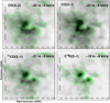 |
Fig. 2 Velocity integrated emission of CO(3−2), CO(2−1), 13CO(2−1), and C18O(2−1). The contour levels are as follows: CO(3−2): 7 to 15 K km s−1 in steps of 2 K km s−1, then in steps of 4 K km s−1 above 15 K km s−1. CO(2−1): 8 to 20 K km s−1 in steps of 3 K km s−1, then in steps of 5 K km s−1 above 20 K km s−1. 13CO(2−1): 2 to 5 K km s−1 in steps of 2 K km s−1. C18O(2−1): 1 to 3 K km s−1 in steps of 0.5 K km s−1, then in steps of 1 K km s−1 above 3 K km s−1. |
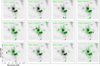 |
Fig. 3 Channel maps of the HCO+ (4−3) emission (green contours) in velocity intervals of 1 km s−1, covering the total velocity interval from −18.6 to −6.6 km s−1 superimposed on the 870 µm continuum emission (grey tonalities). The velocity interval is indicated in the upper left corner of each image. The contour levels are 0.65 (~6 rms), 1.3, 2.5, 3.5, 5, 7, and 9 K km s−1. The bottom right panel shows the emission of the line integrated into the total velocity range. The contour levels are 0.23 (~7 rms), 0.55, 1.2, 1.8, 5, and 7.2 K km s−1. |
3.1.2 Analysis of the ASTE data
To analyze the morphology and velocity of the densest molecular gas in the nebula we used ASTE data, specifically focusing on the HCO+(4−3) line. This transition has been well established as a reliable tracer of dense molecular gas in star-forming molecular clumps (e.g., Paron et al. 2015; Ortega et al. 2017, 2020; Duronea et al. 2017). Additionally, this transition provides the best angular resolution among our dataset, comparable to the 870 µm images (see Table 2), making it best-suited for identifying the molecular counterparts of the AGAL sources.
In Fig. 3, we present the channel maps of the HCO+ (4−3) line emission, which has been superimposed on the 870 µm emission to facilitate the identification of the molecular counterparts of the AGAL sources. Every image represents an HCO+ (4−3) emission integration over a velocity interval of 1 km s−1. In the bottom right panel, we show the line emission integrated over the total velocity range, which matches quite well with that of the C18O(2−1) emission (see Fig. 2). For the sake of the analysis, we identified a collection of HCO+ emission condensations (hereafter “clumps”) that have been designated from A to E. The clumps were selected by eye from the total integrated line emission map and based on the following straightforward criteria: (1) the peak temperature of each clump is at least 5 times the rms noise; (2) the decrease in Tmb between the peak temperature of two adjacent clumps is larger than five times the rms noise; and (3) the clump is detected across at least ~50% of the total velocity range of the molecular cloud. The clumps are indicated in the velocity interval panel at which they reach the maximum emission peak temperature. Clump A becomes first noticeable at a velocity of ~−19 km s−1 (not shown in Fig. 3) achieving its maximum emission in the velocity interval from −16.6 to −15.6 km s−1 and it remains detectable until a velocity of ~−11 km s−1. Clump B becomes detectable at a velocity of −17 km s−1, while clump C at −18 km s−1. Both achieve their maximum emission in the velocity interval from −13.6 to −12.6 km s−1. Clump D is detected in the whole velocity range, achieving its maximum in the velocity interval from −11.6 to −10.6 km s−1. On the other hand, clump E is detected within a narrower velocity range (from −12.6 to −8.6 km s−1), achieving its maximum in the velocity interval from −10.6 to −9.6 km s−1.
In the right panels of Fig. 4, we show the HCO+(4−3) spectra of each clump obtained by averaging their emission over their corresponding area, Aclume, which was defined from a radius that encompasses the emission corresponding to ~50% of their Tmb peak. They were obtained in the direction of the maximum emission peaks in the total velocity integrated map. Then, we set 20″ for clump A, 30″ for clump B, 25″ for clumps C and D, and 27″.5 for clump E. We fitted the obtained spectra with single Gaussians to extract their integrated intensity, ∫ Tmb dυ, central velocity, Vlsr, peak temperature, Tpeak, and the full width at half maximum, FWHM, and the results are presented in Table 3. Additionally, we obtained spectra from the CO(3−2) line data (see left panels of Fig. 4) which have similar angular resolution, and extracted their Gaussian parameters as well.
The central velocities obtained for each clump reveal a velocity dispersion of ~5 km s−1 from the southernmost clump (A) to the northernmost (E). This is depicted more prominently in the first-order moment map (i.e., the intensity-weighted velocity field) presented in Fig. 5. From the figure, we infer that the velocities of the clumps delineate the velocity field of the entire complex, which exhibits a dispersion of up to ~6 km s−1 along its north-to-south extension. This value is typical for giant star-forming molecular complexes (e.g., Román-Zúñiga et al. 2015; Goddi et al. 2016). For comparison with an optically thin transition, in the lower panel of Fig. 5, we also display the first-order moment map of the C18O(2–l) line obtained from the APEX data, revealing a consistent velocity distribution with that of HCO+(4−3).
From the analysis above, it becomes evident that clumps A, B, C, D, and E are the molecular counterparts of ATLASGAL sources AGAL348.649-01.069, AGAL348.726-01.039, AGAL348.701-01.042, AGAL348.698-01.027, and AGAL348.754-01.069, respectively, and robustly confirms the association of all the clumps with the same molecular complex, establishing their physical connection with RCW 122. This enables a further direct comparison of their physical and chemical properties. Then, we will hereafter adopt for the clumps a distance of  kpc, an estimate obtained from the trigonometric parallax of the CH3OH maser associated with AGAL348.701-01.042 (Wu et al. 2012).
As part of the velocity analysis, we also searched for distinctive profile features. Departures from the Gaussian shape may indicate different processes occurring inside a molecular clump, potentially serving as signatures of the star formation process. The profiles in Fig. 4 show that clump A exhibits the most pronounced line wings among the five clumps, indicative of molecular outflow activity. In the top panel of Fig. 6, we present the beam-averaged spectrum obtained at the center of clump A, revealing conspicuous blue and red spectral wings. The bottom panel of Fig. 6 displays a three-color Spitɀer image of clump A where the 3.6, 4.5, and 8 µm wavelengths are depicted in blue, green, and red, respectively. Dashed-white contours delineate the ATLASGAL continuum emission at 870 µm. A point source (WISE J172000.83–390159.3) with associated faint green extended emission is seen projected on the center of clump A which, as mentioned in Sect. 1, suggests potential molecular outflow activity (EGO-like source). However, we are cautious regarding this source as it was not included in the catalog of Cyganowski et al. (2008). The blue and red contours correspond to the CO (3−2) emission integrated between -33 and −20 km s−1, and between −7 and +3 km s−1, respectively (see top panel of Fig. 6), highlighting the presence of blue and red lobes structures (partially detected also in the APEX CO(2− 1) line emission; see Fig. B.1 in Appendix B11). Both lobes align spatially with their emission peaks separated by about 5″, which might indicate that the possible outflow predominantly lies along the line of sight. Therefore, it is expected that the 4.5 µm extended emission of the potentially associated WISE source does not extend significantly along the plane of the sky.
Clumps B, C, and D do not display evident spectral wings, although the CO(2−1) spectrum toward clump B (see Fig. B.2 in Appendix B) shows some incipient features. However, due to the complexity of the region, characterized by numerous substructures and active stellar and protostellar sources (see Sect. 3.3), and considering the limitations imposed by the angular resolution of our molecular data, discerning which source contributes to such gas perturbations requires further investigation. As can be noted from Fig. 4, the HCO+(4−3) spectrum of clump D exhibits a double-peak structure (originated by a relatively pronounced dip at a velocity of ~−12 km s−1) with a slightly brighter peak at more negative velocities. This kind of “blue asymmetry” is usually associated with the infall motions of the gas, which may lead to a self-absorbed emission of an optically thick line (Evans 1999). Nevertheless, this feature is not observed in the CO(3−2) profile, which instead exhibits a “blue skewed” profile. A more comprehensive study of these sources is warranted in future work, utilizing higher-resolution data.
Finally, the CO(3−2) spectra toward clump E show an emerging blue wing (consistent with its CO(2−1) spectra). Given that clump E exhibits a blue shift relative to the other clumps (see Table 3), and the absence of a corresponding red wing, we interpreted this kinematic feature as a potential external perturbation at the clump scale.
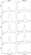 |
Fig. 4 Averaged CO(3−2) and HCO+(4−3) line spectra obtained toward the emission peak of molecular clumps A, B, C, D, and E. The red curves show the Gaussian fits to the lines. Vertical red dotted lines indicate the central velocities from the Gaussian fits. |
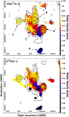 |
Fig. 5 First-order moment maps of the HCO+ (4−3) emission line (upper panel) and C18O(2–l) emission line (lower panel). The black contours represent the ATLASGAL 870 µm emission, as presented in Fig. 1. Black labels and arrows in the upper panel indicate the identified molecular clumps. Color tonalities represent different LSR radial velocities. |
Observed and derived parameters of the clumps and their spectra obtained from the ASTE data.
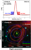 |
Fig. 6 Beam-averaged CO(3−2) spectrum toward the center of the clump A (top). The blue and red wings have been highlighted in their respective colors. Three color Spitɀer image with 3.6, 4.5, and 8.0 µm emissions (bottom) seen in blue, green, and red, respectively. The white contours represent the 870 µm ATLASGAL emission. Levels are at 0.5, 1, and 2 Jy beam−1. The blue and red contours correspond to the CO emission integrated between −33 km s−1 and −20 km s−1 and between −7 km s−1 and +3 km s−1, respectively. They are indicating the possible molecular outflow activity in the line of sight toward clump A. |
3.1.3 Identification of several molecular species from the APEX data
Based on the results reported above, we will now concentrate our analysis on clumps A, B, C, D, and E. We used APEX data to obtain averaged spectra over each clump to analyze the chemical diversity in the clumps and to determine some of their physical properties. The averaged spectra were obtained from the same positions and areas used to extract the HCO+(4−3) and CO(3−2) spectra in Sect. 3.1.2. To identify the lines present in the spectra, we adopted a systemic velocity of ~−14 km s−1 for the Doppler correction, based on the velocities reported from the CS(2−1) and CO(1−0) lines by Bronfman et al. (1996) and Arnal et al. (2008), respectively. We used the CDMS and JPL spectroscopy databases, adapted for use with CLASS. No identification was attempted for the spectra obtained at the frequency tuning of 230.380 GHz since the rms noise was insufficient to detect any molecular line other than CO(2−1). In total, we identified 20 transitions from 11 different molecules. A visual overview of the detected transitions for each clump is presented in Fig. 7 where the identified molecular lines are labeled in red. As indicated in Sect. 2.1.1, no APEX observations were obtained at frequencies between 258 380 MHz and 262 380 MHz in the region corresponding to clumps A and E. Since almost all detected lines exhibit Gaussian profiles, we fitted them with single Gaussians to obtain some of their averaged parameters. They are indicated in Tables A.1 to A.5 in Appendix A. The fits for every transition are shown in Figs. B.1 to B.5 in Appendix B. As noted, clump B is the line-richest and strongest emitter, while clump E is the poorest. Clumps C and D display nearly similar characteristics in the variety and strength of emission lines. In the frequency range between 218 300 MHz and 222 300 MHz, we detected the transitions CH3OH(42,0−31,0), H2CO(32,2−22,1), H2CO(32,1−22,0), and SO(56−45) in clumps A, B, C, and D. Additionally, we detected four rotational transitions of CH3CCH in clumps B, C, and D (130−120, 131−121 132−122, and 133−123). Notably, a strong unidentified transition at ~222 063 MHz is detected in all sources. A wealth of molecular transitions were also detected in the spectra at the frequency range between 258 380 MHz to 262380 MHz. The transitions H13CN(3−2), H13CO+(3−2), HN13C(3−2), CH3OH(21,0−10,0), and SO(67-56) were detected in all the clumps observed at these frequencies (B, C, and D). We also detected transitions of the ethynyl radical CCH in clumps B, C, and D, with both the (F = 4−3) and (F = 3−2) hyperfine components of the (N = 3−2) and (J = 7/2−5/2) transition observed to be blended in all three clumps. Similarly with the hyperfine components (F = 3−2) and (F = 2− 1) of the transition (N = 3−2) and (J = 5/2−3/2). Additionally, we identified the single transitions (N = 3−2) (J = 5/2−3/2) (F = 2−2) and (N = 3−2) (J = 5/2−5/2) (F = 3−3) only in clump B. An absorption feature present at ~258750 MHz is worth noting, likely caused by atmospheric water vapor.
To depict in detail the spatial emission distribution of detected molecular lines, we constructed zeroth-order moment maps (velocity-integrated emission) for each clump. We compared them with the 870 µm continuum distribution maps, which are shown in Figs. C.1 to C.5 in Appendix C12. The maps were generated using the total velocity range where the emission lines are detected. Given that most of the detected molecules serve as reliable tracers of dense to moderately dense gas, the consistent alignment of their emission distribution with the morphology of the optically thin dust continuum emission indicates that the molecular line emission originates predominantly from the clumps rather than the surrounding gas environment. If the molecular gas and dust emissions are optically thin, their column density distribution should mirror their integrated emission since they are tracing the same material. Consequently, their integrated intensity peaks should be observed at the same positions. This is observed in most instances, except for the CO(3−2) and CO(2− 1) emission maps, where the emission peaks appear slightly displaced from the dust emission peaks in all the clumps, particularly in clumps A and E. This discrepancy could be attributed to optical depth effects as evidenced by the more accurate positional coincidence between molecular and dust emission peaks for the optically thinner 13CO(2−1) and C18O(2−1) lines, except clump E. A plausible explanation is that molecular depletion occurs in the cold core of the clump, where the density is higher. Depletion is believed to occur when dust and gas have low temperatures and high density (T ~ 10-20 K, N(H2) > 1022 cm−2). In such regions, the conventional molecular tracers, like CO and its isotopologues, freeze out onto the dust grain resulting in a lack of emission in their molecular lines. However, higher-spatial resolution millimeter observations are necessary to corroborate whether the molecular species detected at clump scales (~1 pc) also trace the inner regions of the clump at core scales (~0.1 pc).
3.1.4 Physical properties of the molecular clumps
CO lines. To estimate some physical properties of the molecular clumps, we used the parameters derived from the Gaussian fit for the CO(2−1) line and its optically thin iso-topologue C18O(2−1) of their integrated emissions presented in Tables A.1 to A.5. Assuming that all rotational levels are thermalized with the same excitation temperature, that is local thermodynamical equilibrium (LTE), and that the emission is optically thick (τ12 >> 1), we derived the excitation temperature, Texc, of each molecular condensation using
![Mathematical equation: ${T_{{\rm{peak }}}}({\rm{CO}}) = T_{12}^*\left[ {{{\left( {{{\rm{e}}^{T_{12}^*/{T_{{\rm{exc }}}}}} - 1} \right)}^{ - 1}} - {{\left( {{{\rm{e}}^{T_{12}^*/{T_{{\rm{bg }}}}}} - 1} \right)}^{ - 1}}} \right],$](/articles/aa/full_html/2024/09/aa49136-23/aa49136-23-eq4.png) (1)
(1)
where  , with ν12 as the rest frequency of the CO(2−1) line and Tbg = 2.7 K. The optical depth of the C18O(2−1) line, τ18, was obtained assuming that the excitation temperature is the same for CO(2−1) and C18O(2−1), and using the expression
![Mathematical equation: ${\tau ^{18}} = - \ln \left[ {1 - {{{T_{{\rm{peak}}}}\left( {{{\rm{C}}^{18}}{\rm{O}}} \right)} \over {T_{18}^*}}{{\left[ {{{\left( {{{\rm{e}}^{{{T_{18}^*} \over {{{\rm{T}}_{{\rm{exc}}}}}}}} - 1} \right)}^{ - 1}} - {{\left( {{e^{{{T_{18}^*} \over {{T_{{\rm{bg}}}}}}}} - 1} \right)}^{ - 1}}} \right]}^{ - 1}}} \right],$](/articles/aa/full_html/2024/09/aa49136-23/aa49136-23-eq6.png) (2)
(2)
where  . We also estimated the optical depth of the CO(2−1) line from the 18CO(2−1) line assuming an abundance ratio CO/C18O ~500. We derived the C18O column density using
![Mathematical equation: $N\left( {{{\rm{C}}^{18}}{\rm{O}}} \right) = 1.252 \times {10^{14}}\left[ {{{{e^{{5 \over {{T_{{\rm{exc}}}}}}}}} \over {1{{\rm{e}}^{ - {{1053} \over {{T_{{\rm{exc}}}}}}}}}}} \right]{T_{{\rm{exc}}}}\int {{\tau ^{18}}} {\rm{d}}\v \left( {{\rm{c}}{{\rm{m}}^{ - 2}}} \right).$](/articles/aa/full_html/2024/09/aa49136-23/aa49136-23-eq8.png) (3)
(3)
Then, we estimated the H2 column density, N(H2)LTE, from N(C18O) adopting an abundance X[C18O] = 5 ×10⁶ (Garden et al. 1991). The obtained values are presented in rows 1 to 5 of Table 4. We also present the optical depths and column densities derived for the 13CO(2−1) line. We estimated uncertainties of about 20 %, arising mostly from calibration uncertainties and the fitting procedure. The total hydrogen mass of each clump (M(H2)LTE; row 6 of Table 4) was calculated using
 (4)
(4)
where msun is the solar mass (~2× 1033 g), µ is the mean molecular weight (assumed to be equal to 2.76), mH is the hydrogen atom mass, and d is the adopted distance. For M(H2) we estimate an uncertainty of about ~30% primarily arising from uncertainties in N(H2)LTE and d.
CH3 CCH lines. Because this molecule is a symmetric rotor, its rotational transitions are characterized by two quantum numbers, J and K, which represent the total angular momentum and its projections on the principal symmetry axis, respectively (the so-called K-ladders). Due to its small electric dipole moment (µ = 0.75 D) and that is optically thin in most typical conditions in massive clumps, rotational transitions of CH3CCH are colli-sionally excited (LTE) at low densities. As a result, the molecule acts as an excellent temperature probe for gas with densities over 105 cm−3; these are values that are more influenced by the inner dense regions of a clump and relatively less so by their outer envelopes, making this molecule a reliable tracer of physical conditions and passive heating (Miettinen et al. 2006; Molinari et al. 2016).
As mentioned earlier in this paper, we detected rotational transitions of CH3CCH only in clumps B, C, and D. To estimate excitation temperatures and column densities, we constructed rotational diagrams (Goldsmith & Langer 1999). Assuming LTE conditions and optically thin emission, this corresponds to the Boltzmann distribution and can be represented as
 (5)
(5)
where Nu/𝑔u is the column density per statistical weight for the upper level u, Eu is the energy of the upper level, Q(Trot) is the internal partition function as a function of the excitation temperature, and Ntot is the total column density. Nu can be estimated from the integrated intensity of the line as
 (6)
(6)
where Cτ = τ|(1e−τ) is the optical depth correction factor. Then, values ln(Nu|𝑔u) versus Eu can be obtained from the observed lines and can be fitted using a straight line, whose slope is defined by the term 1/Texc. Thus, Eq. (5) becomes
 (7)
(7)
We constructed the rotational diagrams using a beam dilution factor ~ 1 (source size ~28″). The optical depth correction was performed iteratively with CASSIS. The internal partition function of CH3CCH has been updated to address more accurate calculations (see Appendix D for details). In the upper panel of Fig. 8 we show the obtained diagrams, as well as the obtained values of rotational temperatures and column densities for each clump. The plotted uncertainties were estimated as ∆(ln(Nu|𝑔u)) = ∆W|W, were W is the integrated area of the line and ∆W is its uncertainty, estimated as13 ∆W = ((cal|100 × W)2 + (rms × (2 × FWHM × ∆v)2))−1, with cal as the calibration error (in percentage), rms the noise around the selected line (in K), FWHM the line full-width half maximum (in km s−1), and ∆υ the velocity bin size (in km s−1 ).
LTE calculations for several line identifications. Except for CH3CCH (as well as for the hyperfine structure of CCH), all other molecular species were identified through either one or two spectral lines. The limitations associated with single- or double-line identifications impede the precision of determining physical parameters (e.g., Roueff et al. 2021).
Despite the above, for the species detected via one or double lines, we applied the Markov chain Monte Carlo (MCMC). The MCMC-LTE algorithm was run within the CASSIS software, representing an iterative computation where a random walk systematically explores the parameter space. Convergence toward optimal solutions within the specified parameter space is achieved by minimizing the χ2 statistic. The advantage of this method arises from its capability to define free parameters, such as column density, excitation temperature, source size, line width, and systemic velocity. The results, corresponding to the χ2 calculation achieved with 103 iterations in a numeric grid, with limits of Texc =10–100 K and N=1012–1016 cm−2, are presented in Table 5. For each molecule, we have included the computed column density and excitation temperature. These results offer an initial and rough estimate of the species under analysis. In subsequent studies, additional and new spectral lines will be needed to enhance the robustness of the calculations.
The detection of previously reported molecules indicates the presence of gas with high temperature and density, conditions required for both their formation and excitation. However, as observed from the estimations above, the derived temperatures appear low. This discrepancy may be explained by the clumpi-ness of the emitting gas. If the gas is not very clumpy, derived H2 volume densities fall below the critical densities of these molecules (i.e., the excitation is sub-thermal and Texc < Tkin). Because estimations derived with APEX data are averaged on parsec-sized scales they may be significantly higher if the gas is clumpy on core-size scales (~0.1 pc). Higher spatial resolution images are necessary to clarify these issues.
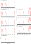 |
Fig. 7 Clump-averaged APEX spectra obtained toward clumps A, B, C, D, and E. Molecular lines detected above 2.5 times the rms are indicated in red. |
Physical properties derived for clumps A to E obtained from carbon monoxide data.
3.2 Dust continuum emission
In Fig. 9, we present the IR emission distribution of the MSX and Herschel bands, which are good tracers of warm and cold dust, respectively, in the region of RCW 122. We overlaid the HCO+(4−3) emission integrated into the total velocity range (as presented in Fig. 3) to associate the emission corresponding to the identified molecular clumps. As the figure illustrates, all five clumps have conspicuous counterparts in all Herschel bands with clumps B and D being particularly prominent. In contrast, only clumps B, C, and D show significant emission in the MSX bands with clump B being especially prominent, while clumps A and E are barely detectable, if any, at all MSX bands. The figure supports the evolutionary grade proposed in Table 1, by showing how differently evolved star-forming clumps change their appearance with wavelength. Namely, the youngest and coldest star-forming clumps (clumps A and E) appear as shadows (or faint diffuse emission) from NIR to MIR wavelengths against the diffuse background. In contrast, at longer wavelengths, the clumps emit significantly above the background emission making them identifiable as prominent emission sources. On the other hand, the hotter clumps (B, C, and D) are bright in all the bands, particularly clump B.
To analyze the overall dust temperature distribution in RCW 122, we initially attempted to utilize density-weighted temperature maps derived using the point process mapping (PPMAP) procedure14 with continuum Hi-GAL data (Marsh et al. 2017). However, since these maps do not cover the entire region of RCW 122, we generated a new color temperature pixel-to-pixel map assuming a standard grey-body model for the emission, as follows:
 (8)
(8)
(Hildebrand 1983), with B(v, T) as the blackbody Planck function (for a frequency v and temperature T), κv the opacity of the emitting dust at the frequency v, Ωbeam the beam solid angle  , and N the dust column density. The opacity, κv, is empirically determined to have a power-law dependence on the frequency as
  with β as the spectral index of the thermal dust emission. For the silicate and graphite dust composition, we have β ~2 (Draine & Lee 1984). However, observations have shown that β can reach values as low as ~ 1 and as high as ~3 (Oldham et al. 1994). In this paper, we adopted the value of β = 1.75. We used the ratio of the 70 µm versus 160 µm Herschel maps, which are better suited to probe color temperatures not too cold (T ≥ 20 K) and up to ~80 K. Besides, the angular resolution of the temperature map obtained using these bands is the highest resolution achievable from the Herschel maps. The 70 µm map was smoothed to match the angular resolution of the 160 µm data. Then, in the optically thin thermal dust emission regime the ratio of the 70 and 160 µm fluxes can be related using
 (9)
(9)
Then, the color temperature map was constructed as the inverse function of the ratio maps namely,  . We show the map in the upper panel of Fig. 10. The uncertainty of this method was estimated to be about ~10–15% (Preibisch et al. 2012). The color temperature map shows a clear systematic gradient from the active central region, at temperatures as high as ~37 K, to the periphery of the complex, at temperatures as low as ~21 K. Peaking maxima temperatures (~35–37 K) are located along several patchy strips. Two of them are located approximately at RA, Dec (J2000)=(17:20:11, −38:57:30) and RA, Dec (J2000)=(17:20:02, −38:57:26), along the external eastern border of clump B, and between clumps B and D, respectively. A third one is located approximately at RA, Dec (J2000)=(17:20:03, −38:58:05), nicely bordering the external northern edges of clumps C and D. They show a relatively good morphological correlation with the Hα emission of the complex (see right panel of Fig. 1) which suggests that the action of the radiation of nearby stars is simultaneously ionizing the molecular gas and heating the dust of the external layers of the clumps. A fourth patch of high dust temperature (~33– 35 K) is located around RA, Dec (J2000)=(17:20:07, −38:57:31) projected toward the center of clump B, and showing a good morphological correlation with both the Spitɀer/IRAC and 3 GHz radio continuum emissions (see left and right panels of Fig. 1). This suggests that the dust in clump B is being internally heated, very likely by the action of central stellar and protostellar objects (see Sect. 3.3). The lowest dust temperatures are observed toward clumps A and E (~21 and ~22 K, respectively), while toward clump C, temperatures are slightly higher (~26 K). Towards clump D temperatures are about 31 K.
Making use of the color temperature and the 870 µm emission maps, we also constructed the pixel-to-pixel H2 column density map, N(H2)870, using Eq. (8) expressed as (Hildebrand 1983):
 (10)
(10)
where R is the gas-to-dust ratio, assumed to be 100, Ω870 is the beam solid angle of the 870 µm observations, and k870 is the dust opacity per unit mass at 870 µm, assumed to be 1.85 cm2 g−1, estimated as the average of all dust models from Ossenkopf & Henning (1994) for a dust spectral index of 1.75 (König et al. 2017). The N(H2) map is shown in the lower panel Fig. 10. As expected, a clear gradient is noticed from the center of the complex to its periphery. The highest peak density is observed toward the center of clump B (~3.5 × 1023 cm−2), while toward the center of clumps C and D column densities are a bit lower, of the order of ~1.6 × 1023 cm−2. Toward clumps A and E, maxima column density is about ~5 × 1022 cm−2. We obtained beam-averaged peak column densities from the map shown in Fig. 10 using a beam size of ~28". The obtained values are 7.2 × 1022 cm−2, 4.1 × 1023 cm−2, 2.2 × 1023 cm−2, 1.9 × 1023 cm−2, and 7.1 × 1022 cm−2 for clumps A, B, C, D, and E, respectively. We also derived source-averaged column densities over the circular areas adopted for HCO+(4−3) clumps (see Sect. 3.1.2). The obtained values are 5.9 × 1022 cm−2, 2.3 × 1023 cm−2, 1.6 × 1023 cm−2, 1.4 × 1023 cm−2, and 5.1 × 1022 cm−2, for clumps A, B, C, D, and E, respectively. Using the latter values we derived the mass (gas+dust) values for the clumps (M870) using Eq. (4), which are indicated in column 14 of Table 6. It should be noted that pixels at the center of clump D are blanked. Therefore, both the column densities and masses derived using this map are almost certainly lower limits.
The IR spectral energy distribution (SED) analysis is a powerful tool for studying stellar and protostellar objects and star-forming clumps, potentially allowing for their classification from an evolutionary standpoint. A comprehensive survey and analysis were conducted by Urquhart et al. (2018) over approximately 8000 ATLASGAL sources in the Galactic disk. They obtained SEDs using 870 µm emission and publicly available MIR and FIR data. While the survey covered the region of RCW 122, unfortunately, AGAL348.726-01.039 (clump B) was not included in the study. Given the observational evidence outlined so far, which suggests that clump B is likely the most evolved, its corresponding SED could provide significant insights for the current analysis. Thus, in this study, we obtained the SED for clump B. To ensure consistency, we applied the same procedure to the remaining clumps, enabling a viable comparison of their properties. Black-body models were adopted for the warm component, while grey-body models were utilized for the cold component, incorporating data from the MSX and Herschel-PACS+870 µm bands, respectively. To obtain fluxes in each band of the used surveys, we employed the circular aperture determined from the HCO+ emission which served for the identification of clumps A to E. Background subtraction was performed by averaging and cropping emissions for each band as determined in five positions far away from the complex. We assumed uncertainties of approximately 15% for flux densities to account for the intrinsic instrument error and source extraction. The obtained fluxes are presented in Columns 2 to 11 in Table 6. For the SED fitting, we used the nonlinear least-squares Marquardt-Levenberg algorithm adapted for use with the GNUPlot graphing utility. In Fig. 11, we show the fitted SEDs, while the obtained temperatures for the cold components are presented in Column 12 of Table 6. We found that the lowest temperatures (23.7 and 25.6 K, corresponding to clumps A and E, respectively) are higher than those typically expected for quiescent starless clumps, namely IRDCs, whose temperature is mainly determined by cosmic ray heating (~ 10 K; Urban et al. 2009). Further, the existence of a warm component (albeit weak for clumps A and E) suggests that all five clumps are being internally heated to different degrees, particularly in those that appear to be more evolved, namely, clumps B and D.
Although a warm component can be fitted for the clumps, only the luminosities of these components are useful parameters, while masses and temperatures are poorly constrained due to optical depth effects, especially at shorter wavelengths. To estimate the luminosities for each clump, we used a PHYTON code to obtain the integrated flux from the fitted SED models using
 (11)
(11)
where Sλ is the flux density function derived from the fitting and d the adopted distance for the clump. The obtained luminosities for cold and warm components (green lines in Fig. 11) were used to determine the total bolometric luminosity (Lbol) by integrating over the entire SED. The obtained values are presented in Column 13 of Table 6.
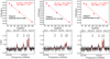 |
Fig. 8 Rotational diagrams obtained with the K-ladder (13–12)(K = 0,1, 2,3) of CH3CCH for clumps B, C, and D (top). Observed spectra of CH3CCH (black lines) overlaid on the synthetic spectra (red lines) obtained with the physical parameters derived from the rotational diagrams (bottom). |
Column densities (N, cm−2) and excitation temperatures (Texc, K) derived from LTE-MCMC calculations and rotational diagrams for the species detected in clumps A to D.
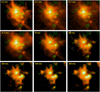 |
Fig. 9 HCO+(4−3) emission as presented in Fig.3 (green contours) superimposed on the four MSX and Herschel bands emissions (red tonalities). |
Obtained flux densities and physical parameters derived from MIR and FIR emissions for clumps A to E.
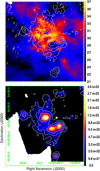 |
Fig. 10 Dust color temperature (K) map derived from the 70 and 160 µm emissions (upper panel) and column density (cm−2) map derived from the 870 µm map emission (lower panel). White contours underline the HCO+(4−3) emission map as presented in Fig. 3. The color temperature and column density color bar scales are on the right, expressed in K and cm−2, respectively. |
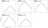 |
Fig. 11 Spectral energy distributions derived for clumps A to E using a two-component black-body and grey-body model (green lines). The blue lines represent the total SED. The plots are on a logarithmic scale. |
3.3 Stellar population analysis and star formation
To unveil the stellar population associated with DBS 119, we selected a circular region of 5′ in radius centered on the molecular complex (see middle left panel of Fig. 12) aiming to encompass the majority of the probable cluster members. The location and size of the studied region were determined through an iterative process, identifying star overdensities in the VVV NIR image (not presented here) and maximizing the inclusion of probable members using our photometric method. Photometric two-color and color-magnitude diagrams (TCD and CMD, respectively) of the brightest (J < 16) point objects located in the selected circular region are presented in the upper panels of Fig. 12. Both diagrams reveal the presence of an important differential reddening. We analyzed the diagrams and classified the objects following a procedure based on the computation of several reddening-free parameter values (see Baume et al. 2020 and Corti et al. 2023 for details). Thus, we made a photometric selection of early main sequence (MS) stars and objects with IR color excess (YSO candidates). For the procedure we used, as a reference, the MS values given by Sung et al. (2013) and Koornneef (1983). We also considered a normal interstellar reddening law (RV = AV/EB–V = 3.1) and the reddening model given by Wang & Chen (2019). Given that the upper MS exhibits an almost vertical shape over the IR CMD, it did not allow us to estimate precise distance values. Therefore, we opted for the previously mentioned value of 3.38 kpc (see Sect. 3.1.2). On the other hand, the obtained CMD could provide an estimation of the foreground color excess (minimum color excess value) of the studied young stellar population. Hence, we derived a corresponding EB–V = 2.8, considering a normal reddening law. Therefore, the adopted extreme values for color excesses are in the range E(B–V) = 2.8–8.8. Both border values were used to identify MS stars, while only the lower one was used to select objects with IR color excess. Ranges for color indices excesses at NIR bands were computed using the Wang & Chen (2019) model. The border values are also indicated in the photometric diagrams by the location of the shifted MS (at the minimum value) and the point of the reddening vector (reaching the maximum value).
The spatial distribution of selected objects is presented in the middle left panel of Fig. 12, superimposed on the total HCO+(4−3) emission as presented in the last panel of Fig. 3. A conspicuous overdensity of stellar and protostellar source candidates, likely members of DBS 119, is discernible at the center of the molecular complex. Particularly, a compact cluster of sources, namely sources #2, 7, 8, 12, 14, 15, 17, and 18, appears projected toward the denser regions of clump B, coincident with the bright arc-like structure observed in the 8 µm and 3 GHz emissions (see the zoomed-in region in the bottom-right panel of Fig. 12). Spatially coincident with the radio continuum and HCO+(4−3) emissions, these sources likely play a crucial role in internally heating the dust and ionizing the gas, leading to the formation of an embedded HII region at the densest part of the clump, as traced by the HCO+(4−3) emission peak. The multiple stellar and protostellar sources’ positional coincidence with these emissions suggests that the molecular dispersion and dissociation phase has not definitively started within the clump. This alignment provides additional confirmation that the HII region is still at an early stage, potentially close to the UCHII phase as suggested in Sect. 1, although seemingly more evolved than that observed in clump D (see below).
Another concentration of sources, including sources #1, 4, 5, 6, 11, 13, 22, 23, 25, 27, and 28, is noticeable toward the central region of the complex, encompassing clumps C and D, especially at the interstices between them, and between clump B (see the zoomed-in region in the bottom-left panel of Fig. 12). These sources may be responsible for ionizing the gas in this region, giving rise to the bright Hα emission, as suggested in Sect. 3.1.1. Furthermore, the YSO candidate #25 appears projected at the center of clump D, almost coincident with the HCO+(4−3) emission peak. Without access to additional information, we can speculate that this protostellar source is responsible for the UCHII identified at the center of the clump (see Sects. 1 and 3.1.1).
The location of adopted cluster members in the photometric diagrams allowed us to estimate their absolute magnitude (MV) and absorption (AV) (see e.g., Roman-Lopes 2007; Baume et al. 2020). This procedure is approximate as it assumes each object to be a main sequence star and neglects the influence of emission lines or IR excess. Since most emission features are present in the K band, we minimized this effect by dereddening the location of each star in the J vs. J − H diagram. The results of these estimations are presented in the middle right panel of Fig. 12. It is evident that objects primarily associated with clumps B and D exhibit high absorption values (AV ≳ 14–15) and tend to be the most luminous, likely of the OB-type. For isolated objects, their high absorption values could stem from intrinsic factors, local variations in interstellar dust, or the potential invalidity of the main sequence star assumption in these cases.
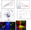 |
Fig. 12 Studied region of RCW 122. Upper panels: IR photometric diagrams for those sources with J < 16 and located inside the 5′ radius around the center of the complex. Gray symbols indicate no classified stars, most of them are likely to be field population. Green and blue curves are the MS (see text) shifted according to the adopted distance modulus with and without absorption/reddening, respectively. The dashed blue curve in the CMD is the 1 Myr isochrone for z = 0 : 02 from Siess et al. 2000. Red lines indicate the considered reddening path. The location of the shifted MS and the reddening vector indicates the adopted range in color excess. Green symbols correspond to MS stars and red ones correspond to stars with probable IR excess. Middle left panel: total velocity integrated HCO+(4−3) emission levels as presented in Fig. 3. Clumps A to E are indicated in black labels. The black dashed circle indicates the 5’ radius adopted for the cluster. Symbols are considered cluster members. Middle right panel: absolute magnitudes (MV) vs. absorptions (AV) obtained from the photometric diagrams (see text). Lower panels: zoom-in view of the central regions of clump B, C, and D. Red, green, and blue tonalities depict 8 µm, 3GHz continuum, and Hα emissions, respectively, while white contours represent the HCO+(4−3) emission as presented in the middle left panel. |
4 Discussion
In Sect. 1, we summarize some of the most prominent observational features of the star-forming complex RCW 122, particularly on the sources AGAL348.726-01.039, AGAL348.701-01.042, AGAL348.698-01.027, AGAL348.754-01.069, and AGAL348.649-01.069. We have built a tentative classification system according to a simple evolutionary scenario. In Sect. 3.1.2, we identify the molecular clump counterparts of these sources using the high-density gas tracerHCO+(4– 3) and determine their main physical and chemical properties through a comprehensive variety of millimeter and submillime-ter data. Given that the clumps have been confirmed to be part of the same complex, we are investigating structures originating from the same parental molecular cloud with similar initial conditions, enabling a direct quantitative comparison of their properties.
The physical properties and derived quantities obtained from the molecular and dust continuum emission (temperature, bolo-metric luminosity, mass, column density, chemical diversity, etc.) are differently suited to distinguish between the evolutionary phases of massive star formation. However, it is acknowledged that discernible trends are more likely to be observed in a larger sample of sources. Moreover, the evolution in the high-mass star formation regime occurs in short timescales in clustered environments, potentially blurring the delineation between different evolutionary phases (Zinnecker & Yorke 2007; Gerner et al. 2014). Nevertheless, a comparative analysis of the physical properties of the molecular clumps identified in RCW 122 (hence, among the AGAL sources) remains instructive and contributes significantly to the overall discussion.
4.1 Luminosity, mass, and temperature
It is known that the luminosity-mass ratio (L/M) can be used in the low- and high-mass star formation regimes as an evolution indicator for protostellar molecular clumps (e.g., Saraceno et al. 1996; Molinari et al. 2008, 2010; König et al. 2017; Giannetti et al. 2017; Urquhart et al. 2018). In essence, during the accretion phase, the YSO accretes mass and increases its luminosity, leaving the mass of the parent clump almost unchanged; then, during the dispersal phase, the YSO reaches its final mass and starts dissociating the nearby molecular gas. Then, the L/M ratio of a star nursery embedded in a molecular clump should increase as the protostar evolves. In addition, it is also expected that a large amount of energy, both radiative and mechanical, emitted by the nascent protostar will progressively heat its surroundings, thus raising the gas and dust temperatures.
Hence, utilizing the obtained values of bolometric luminosities, in conjunction with mass estimations derived from the 870 µm emission map (considered the most reliable method in this study), we computed the L/M ratios for clumps A through E. These ratios were then plotted in increasing order, as illustrated in Fig. 13a. The figure reveals a broad discernible trend in the L/M ratio, consistent with the proposed evolutionary sequence outlined in Sect. 1 for the AGAL sources corresponding to the molecular clumps: A→E→C→D→B. However, the L/M values are closely matched (within uncertainties) between clumps D and B, as well as between A and E. This proximity suggests that these sources are undergoing similar evolutionary stages. Nevertheless, it is important to note that the lower limit value of M870 for clump D likely leads to an overestimation in L/M. This implies that clump B is more evolved, as previously suggested in Sect. 1 and supported by the analysis in Sect. 3. Additionally, some observational features outlined in Sect. 3 indicate that clump A may be more evolved than clump E, contrary to what is broadly inferred from Fig. 13a (see details below).
Our results also reveal a general trend of increasing dust and CH3CCH rotational temperatures, which are the most reliable temperature determinations obtained in this work, with an increasing L/M ratio that is consistent with the proposed evolutionary sequence, as seen in Fig. 13b. The strong correlation between the observed increasing L/M ratios and temperatures broadly confirms the proposed evolutionary sequence for the molecular clumps (and their AGAL counterparts), supporting the working hypothesis that higher L/M values are associated with a more advanced evolutionary stage. Similarly, the proximity of clumps D and B in the plot is notable, owing to minor discrepancies, within the margin of errors, in their molecular and dust temperatures. Furthermore, as CH3CCH is a reliable temperature probe of gas with densities characteristic of the inner envelopes of clumps and hot cores (see Molinari et al. 2016; Giannetti et al. 2017), the lack of spectral lines of this molecule in clumps A and E is indicative of lower temperatures (compared with clumps B, C, and D), either in the core or its inner envelopes, as previously corroborated from previous temperature determinations. The presence of a weak warm component in the SEDs of clumps A and E implies some internal heating within these regions. However, the energy input from internal sources, while generating detectable submillimeter flux, may not be sufficient to significantly increase the bolometric luminosity and the internal temperature of the clumps (estimated to be ~22–25 K). Consequently, this limited energy may insufficiently promote desorption of the CH3CCH molecule from grain surfaces, resulting in non-detections of its spectral lines (Miettinen et al. 2006; Molinari et al. 2016). This suggests that thermal internal activity is relatively low within these clumps, indicating an early evolutionary stage, most likely HMPO. It is worth recalling the EGO-like source embedded at the center of clump A, which is highly probable to be responsible for initiating the molecular outflow detected in the CO(3−2) emission (see Sect. 3.1.2). Then, the protostellar source driving the outflow might be too young to impact significantly on the physical characteristics of the clump at large scales (temperature, ionization conditions, etc.). On the other hand, the internal energy produced at the core of the seemingly more evolved clumps for which the transitions of the CH3CCH were detected (clumps B, C, and D) seems to be raising the temperature of the inner envelope dust and gas to at least ~30–35 K. This is indicative of more intense activity within the clumps. The number of IR sources (either MS or YSO candidate members of the embedded cluster DBS 119) identified mostly in the direction of clumps B and D (Sect. 3.3) is certainly consistent with this scenario. In Fig. 13c, we also show a clear tendency to increase the H2 column density (derived from the 870 µm emission) with increasing L/M ratio; this is additional support to the proposed evolutive sequence for the AGAL sources (thereby the molecular clumps), except for clump D, which appears to be a bit lower than in clump C. However, as previously remarked, the column density derived from the 870 µm emission for this clump is a lower limit.
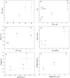 |
Fig. 13 (a) Luminosity-mass ratio of the clumps arranged in the proposed evolutionary sequence. (b) Luminosity-mass vs. temperature determined from CO, submillimeter, and CH3CCH emissions. (c) Luminosity-mass vs. column density determined from CO and submillimeter emissions. (d) 870 µm peak flux density vs. CCH integrated intensity. (e) Column density plot of H13CO+ vs. CCH. (f) Full width at half maximum plot of H13CO+(3−2) vs. CCH(35/2.3–23/2.2). |
4.2 Chemical richness
Molecular species formed and destroyed during the formation of new stars can be used to diagnose the evolution of the star-forming process (Gerner et al. 2014; Urquhart et al. 2019). The chemical evolution of star-forming regions starts with simple and common molecules (like H2, CO, HCO+, etc.), evolving to more complex (even organic) molecules in the HMC phase and ultimately being destroyed in the close environs of the new star, once the HII region is formed. Then, the “richness” of molecular species is a suitable probe for the evolutionary stage of the clumps and a comparison among their properties could be used as a “chemical clock” (e.g. Beuther et al. 2007; Gerner et al. 2014; Immer et al. 2014; Yu & Wang 2015; Hacar et al. 2020). The analysis for this study remains incomplete due to the limited frequency coverage observed for clumps A and E with APEX (see Sect. 2.1.1). Furthermore, APEX data are sensitive to size scales of approximately ~1 pc, considerably larger than the typical size scales of objects such as HMCs (~0.1 pc). This limitation restricts a comprehensive examination of the immediate molecular surroundings of protostellar cores.
Foremost, it is notable that clump A exhibited a richer chemical composition compared to clump E, where only CO and HCO+ transitions were detected, along with an unidentified transition at 222 063 MHz. Despite the absence of CH3CCH lines in both clumps, indicative of relatively simple chemistry likely due to prevailing low temperatures, clump A notably emitted significant levels of H2CO, CH3OH, and SO. Again, this would indicate a relatively more advanced evolutionary stage for clump A, as compared to clump E, which is in contrast to that hinted from the previous L/M analysis. Since several transitions of these molecules are known to be tracers of different components of a protostellar object, such as the outer cold envelope to the jet and outflows, typically at size scales of between 100400 au (Tychoniec et al. 2021), this might serve as additional confirmation of outflow activity at the center of the clump. However, we approach this matter with caution since observations with better spatial resolution are necessary to explore smaller spatial sizes (core scale) and to corroborate whether the detected molecules are ubiquitous at clump size scales or are specifically associated with the immediate surroundings of a hypothetical EGO-like powering source. Considering the relatively low luminosity of the clump (see Sect. 3.2), it is reasonable to reaffirm clump A as a young HMPO clump. The absence of spectral lines besides CO and HCO+ in clump E suggests lower temperatures in the core, with an internal heating source unable to release other simple molecules (such as H2CO and CH3OH) into the gas phase. This indicates, again, an earlier evolutionary phase than clump A, likely representing an intermediate stage between IRDC and HMPO.
For the case of clumps B, C, and D, the variety of molecular transitions detected with APEX is quite comparable, indicating their chemistry is similar (at least on clump scales). The presence of these molecules hints at a heating source (as previously suggested) capable of driving the formation of the molecular species. Particularly in the case of CCH, detecting its transitions toward all three clumps is noteworthy. Although CCH is ubiquitous, even in cold regions, its abundance is known to be enhanced in the molecular gas exposed to UV radiation; then, its emission may trace irradiated regions, such as PDRs (Nagy et al. 2015, and references therein). Therefore, the detection of CCH may be evidencing the effects of internal or external UV irradiation and may be tracing: (1) internal cavities and PDRs associated with the young HII regions embedded in the clumps, or (2) the activity of OB stars ionizing the outer layers of gas within the clumps (Ortega et al. 2020; Tychoniec et al. 2021). In this context, as shown in Tables A.2, A.3, and A.4, velocities of the transitions CCH(37/2,4–25/2,3) and CCH(35/2,3–23/2,2) detected toward clumps B, C, and D present the largest blue shift relative to the rest of the molecular lines. This may indicate that a common mechanism, probably as a result of the powerful winds originating from the massive stars identified in the region inter-clump (see Sect. 3.3), could be affecting the kinematics of the CCH transitions that are probably mapping the external irradiated layers of the clumps. In the case of the CCH(35/2,2–23/2,2) and CCH(35/2,3–25/2,3) transitions, detected only toward clump B, no shift in velocity is observed relative to the other molecular transition. Thus, their detection could indicate extreme environmental conditions of the internal irradiated gas related to the clump, but less kinematically influenced by stellar sources found in the region inter-clump. This interpretation is also in line with the highest temperature and luminosity found toward this clump, likely as a result of the intense activity of multiple newly born stellar and protostellar objects immersed in the clump (Sect. 3.3). However, as previously remarked, the complexity of the region, coupled with the limitations imposed by the angular resolution of our molecular dataset, precludes us from definitively determining the underlying scenario. The above CCH emission aspects will be addressed in an upcoming study utilizing improved angular resolution data (Ortega et al., in prep.).
Although the variety of molecular species reported in this work is relatively scarce, they are commonly detected in star-forming regions (e.g., Sanhueza et al. 2012; Giannetti et al. 2017; Urquhart et al. 2019) and they can give a good glimpse into searching for differences in the chemistry as a function of the evolutionary stage of star-forming molecular clumps. Recently, Martinez & Paron (2024) conducted a molecular line study of HNC, HCN, H13CO+, HC3N, N2H+, and CCH on a sample of 55 sources representing massive star-forming objects at different evolutionary stages (IRDCs, HMPOs, HMCs, and UCHII,s), aimed to complement the results of Yu & Wang (2015). The authors focussed their analysis on using these molecules as chemical clocks and reported some results that contribute significantly to our analysis. They reported a clear increase in the integrated intensities of N2H+, CCH, HNC, and HC3N with the 870 µm peak flux, which correlates with the evolutionary scheme IRCD→HMPO→HMC. Based on the fact that the H13CO+ column density reflects the amount of H2 in a clump because its abundance does not vary much in time (Nomura & Millar 2004; Yu & Wang 2015), the authors also compared N(CCH) with N(H13CO+). They also found an increment with a conspicuous correlation with the evolutive progression from IRDC to UCHII in which the position of each kind of source appears sectorized. The authors also compared the molecular line widths (FWHM), which are usually associated with the kinematics of the molecular gas (shocks, outflows, turbulence, etc.), and they found that the FWHM increases until they reach the HMC stage (likely as a consequence of the gas dynamics related to the star-formation process). Given these results, in Figs. 13d we show the integrated intensity of CCH vs the 870 µm peak flux values (not included in Table 6) for clumps B, C, and D in which a trend (sharp for clump B, and subtle for clumps C and D) can be discerned according to the proposed evolutionary sequence. Integrated line flux and 870 peak flux values for clumps D and B (proposed as UCHII sources), range between evolutive~9–16 K km s−1 and ~ 10–21 Jy beam−1, respectively, in agreement with those of Martinez & Paron (2024), although their distribution seems not to be tightly sectorized for these kinds of objects (UCHII). A similar configuration is observed in the plot N(CCH) vs. N(H13CO+) for clumps B, C, and D (Fig. 13e), although in this case, the column density values are almost two orders of magnitude lower than those presented by Martinez & Paron (2024) for the HMC and UCHII groups (obtained from Gerner et al. 2014). In the case of the FWHM(H13CO+) vs. FWHM(CCH) plot (Fig. 13f), the trend is more clear and correlates nicely well with the proposed evolutionary sequence, although obtained linewidths for clumps B and D (~3.9 and 3.7 K km s−1, respectively) are quite lower than those presented by Martinez & Paron (2024) for UCHII sources. In addition to broadly validating the proposed evolutionary stages for clumps B, C, and D, Figs. 13d, e, and f provide further confirmation that clump B is the most evolved among them.
5 Summary and concluding remarks
With the aim to improve the analysis of the molecular and dust components associated with the star-forming complex and HII region RCW 122 and to better comprehend the physical and chemical conditions prevailing in massive star-forming regions, we used molecular data collected with the APEX and ASTE telescopes, complemented with available data at different wavelengths. Our study is focused specifically on the analysis of the ATLASGAL sources AGAL348.726-01.039, AGAL348.701-01.042, AGAL348.698-01.027, AGAL348.754-01.069, and AGAL348.649-01.069. These sources appear to be at different evolutionary stages, as inferred from multiple emission features at various wavelengths.
Using ASTE data of the high-density tracer HCO+(4−3) line and the complementary CO(3−2) line, we successfully identified the molecular counterparts (designated as clumps A, B, C, D, and E) of the ATLASGAL sources. These clumps were observed at velocities ranging between ~−15 km s−1 and −10 km s−1 evidencing a slight velocity dispersion of the whole molecular complex. We verified that all clumps are members of the same molecular star-forming complex, allowing for a direct comparison of their properties. Using CO(2−1) and C18O(2−1) APEX data, we estimated the total LTE mass off the clumps, which range from 200 M⊙ (clump A) to 4400 M⊙ (clump B). We also identified 20 transitions involving 11 molecules, detected in varying proportions within the molecular clumps. Specifically, the K-ladder (J = 13−12) (K = 0.1.2.3) of the molecule CH3CCH was observed in clumps B, C, and D (AGAL348.726-01.039, AGAL348.701-01.042, and AGAL348.698-01.027, respectively), but remain undetected in clumps A and E (AGAL348.649-01.069, and AGAL348.754-01.069, respectively). This indicates low internal temperatures and provides additional evidence of an early stage in the evolution of clumps A and E. The detection of a molecular outflow in the CO(3−2) line, potentially traced by H2CO, CH3OH, and SO lines, likely powered by an EGO-like source identified at the center of clump A, implies that this clump might be in the HMPO phase. Conversely, clump E may be in an earlier (albeit not quiescent) phase, resembling late IRDC or else incipient collapsing HMPO. While the variety of molecular species detected in clumps B, C, and D is quite similar, it is noteworthy that two higher-energy transitions of the molecule CCH were exclusively detected in clump B at different velocities, which may be tracing internal regions of the clump. This suggests that clump B is undergoing a more evolved stage in its evolution, compared with the other two clumps. The rotational temperatures derived from CH3CCH lines for clumps C, D, and B (~29 K, ~36 K, and ~37 K, respectively) indicate that clumps B and D are hotter, a finding consistent with the presence of embedded young HII regions. This inference is supported by the detection of 3 GHz radio continuum emission toward both clumps. In the case of clump D, the HII region appears to be undergoing the UCHII phase, as evidenced by its size and electron density. Conversely, IR photometric data suggests that the ionization of clump B might be powered by multiple stellar and protostellar objects, likely members of the open cluster DBS 119, indicating the complexity of the clump and supporting the scenario of a more evolved evolutionary stage. Clump C, on the other hand, appears to be in an earlier phase, most likely an HMC, just before entering the UCHII stage.
Using MIR-FIR data, we constructed SEDs for all clumps. This enabled us to estimate their bolometric luminosities and temperatures, spanning 1.7×10³ L⊙ and 23.7 K (clump A) to 2.4×10⁵ L⊙ and 33.9 K (clump B). We also determined the total (dust+gas) mass values for the clumps, ranging from 350 M⊙ (clump A) to 3800 M⊙ (clump B). The luminosity-mass ratios obtained for the clumps strongly suggest an evolutionary sequence A/E→C→D/B that is roughly in agreement with the inferred evolutionary sequence of their AGAL counterparts. The progression in temperature and column density, as well as certain properties of the H13CO+ and CCH lines, supports this sequence, with clump B appearing to be in a more advanced stage with respect to clump D.
The observational evidence also suggests the existence of more evolved regions within the complex. The identification of strong Hα spots, coupled with the observation of regions exhibiting high dust temperatures between and in the outer regions of AGAL348.726-01.039, AGAL348.698-01.027, and AGAL348.701-01.042 suggests that some molecular clumps may have evolved into the dispersal/dissociation phase, beyond the UCHII phase. These regions appear to have developed into fully formed HII regions within specific gaps of the molecular complex and they might be powered by several stellar source members of DBS 119, identified at several spots on the interstices between molecular clumps B, C, and D.
Data availability
Appendices B and C are available at https://doi.org/10.5281/zenodo.12706494/.
Acknowledgements
We would like to thank the anonymous referee for his/her helpful comments and suggestions that led to the improvement of this paper. N.U.D. acknowledges support from CONICET grant PIP 112−201701−00507. L.B., R.F., and M.M. acknowledge support from ANID Basal FB210003. M.M. acknowledges support from ANID, Programa de Astronomía - Fondo ALMA-CONICYT, project 3119AS0001. GLB and RG acknowledge support from grant PICT 2019-0344. E.M. acknowledges support under the grant “María Zambrano from the University of Huelva funded by the Spanish Ministry of Universities and the “European Union NextGenerationEU". This project has also received funding from the European Union’s Horizon 2020 research and innovation program under Marie Sklodowska-Curie grant agreement No. 872081 (M.C.), grant PID2022-136228NB-C21 (M.C.) funded by MCIN/AEI/10.13039/501100011033, and, as appropriate, by “ERDF A way of making Europe”, the “European Union”, or the “European Union NextGenerationEU/PRTR”. E.M. and M.C. also acknowledge the support of the Consejería de Transformación Económica, Industria, Conocimiento y Universidades, Junta de Andalucía and European Regional Development Fund (ERDF 2014-2020) by grant PY2000764.
Appendix A Detected transitions and fitting parameters
Transitions detected in clump A and their parameters derived from Gaussian fits
Transitions detected in clump B and their parameters derived from Gaussian fits
Transitions detected in clump C and their parameters derived from Gaussian fits
Transitions detected in clump D and their parameters derived from Gaussian fits
Transitions detected in clump E and their parameters derived from Gaussian fits
Appendix D Internal partition function of CH3CCH
In this work, we have updated the values of the rovibrational partition function, Q(T), of propyne (CH3CCH), a symmetric top molecule with a molecular symmetry group C3v(M) (Bunker & Jensen 1989), at different excitation temperature T (Carva-jal et al. 2019; Carvajal et al. 2024). This is computed as the product of the rotational contribution Qгot(T), defined as a direct sum, and the harmonic approximation of the vibrational partition function Qvib(T) (Carvajal et al. 2019; Carvajal et al. 2024):
 (D.1)
(D.1)
 (D.2)
(D.2)
 (D.3)
(D.3)
where  , and
, and  in Eq. (D.2) are the energy for the i-th rotational state, its rotational angular momentum, and the nuclear spin degeneracy of the energy level i, respectively. In Eq. (D.3) N and
  are the number of vibrational fundamentals and their energies, respectively. In this case, the rovibrational energy levels are referred to the ground vibrational state.
The nuclear spin statistical weights  in Eq. (D.2) take the same value for three possible irreducible representations of the states A1, A2 and E (Bunker & Jensen 1989). In this work, we have considered the same value 𝑔ns = 2 than in CDMS catalog (Endres et al. 2016). Therefore, the nuclear spin degeneracy of the rotational states are those given in Table D.1.
In Table D.2, the values of the rotational partition function (D.2), the harmonic vibrational approximation (D.3) and the rovibrational partition function (D.1) are given. The direct sum of the rotational partition function is calculated from the CDMS rotational energies predicted up to J = 130 and K = 21. The vibrational partition function is computed using the harmonic approximation considering the fundamentals from El Idrissi et al. (2001). The uncertainties of the rovibrational partition function (Carvajal et al. 2019) are computed considering the uncertainties of the rotational and vibrational energies as 10−6 cm−1 and 1 cm−1 , respectively.
The calculated values of the internal partition function of propyne are compared with the ones given in the CDMS catalog, which takes into consideration the lowest vibrational bands v10 = 1, v9 = 1 and v10 = 2 (Endres et al. 2016). It can be noted that no values below 9.375 K and above 300 K have been reported before. In addition, it should be highlighted that the results of this work are comparable with the values of the CDMS catalog up to 225 K. From this temperature up, the results of this work improve considerably the values reported in the CDMS catalog.
In summary, the internal partition function of propyne has been updated incorporating new values below 9.375 K and above 300 K as well as the uncertainties. In addition, the rotational, vibrational, and rovibrational partition functions up to T = 500 K using a 1 K interval are reported as supplementary material.
Nuclear spin statistical weights of the main isotopologue of propyne associated with the rotational states*.
Rotational, vibrational, and rovibrational partition functions for CH3CCH. Comparison between the values obtained in the present work and those published in CDMS catalogue*.
References
- Arnal, E. M., Duronea, N. U., & Testori, J. C. 2008, A&A, 486, 807 [NASA ADS] [CrossRef] [EDP Sciences] [Google Scholar]
- Baume, G., Corti, M. A., Borissova, J., Ramirez Alegria, S., & Corvera, A. V. 2020, New A, 79, 101384 [NASA ADS] [CrossRef] [Google Scholar]
- Belloche, A., Müller, H. S. P., Menten, K. M., Schilke, P., & Comito, C. 2013, A&A, 559, A47 [NASA ADS] [CrossRef] [EDP Sciences] [Google Scholar]
- Beltrán, M. T., Cesaroni, R., Rivilla, V. M., et al. 2018, A&A, 615, A141 [Google Scholar]
- Benjamin, R. A., Churchwell, E., Babler, B. L., et al. 2003, PASP, 115, 953 [Google Scholar]
- Beuther, H., Schilke, P., Sridharan, T. K., et al. 2002, A&A, 383, 892 [NASA ADS] [CrossRef] [EDP Sciences] [Google Scholar]
- Beuther, H., Churchwell, E. B., McKee, C. F., & Tan, J. C. 2007, in Protostars and Planets V, eds. B. Reipurth, D. Jewitt, & K. Keil, 165 [Google Scholar]
- Beuther, H., Henning, T., Linz, H., et al. 2010, A&A, 518, A78 [Google Scholar]
- Braz, M. A., & Epchtein, N. 1983, A&AS, 54, 167 [NASA ADS] [Google Scholar]
- Bronfman, L., Nyman, L. A., & May, J. 1996, A&AS, 115, 81 [Google Scholar]
- Bronfman, L., Garay, G., Merello, M., et al. 2008, ApJ, 672, 391 [NASA ADS] [CrossRef] [Google Scholar]
- Bunker, P. R., & Jensen, P. 1989, Molecular Symmetry and Spectroscopy (Ottawa: NRC Research Press) [Google Scholar]
- Carvajal, M., Favre, C., Kleiner, I., et al. 2019, A&A, 627, A65 [NASA ADS] [CrossRef] [EDP Sciences] [Google Scholar]
- Carvajal, M., Favre, C., Kleiner, I., et al. 2024, A&A, 685, A1 [NASA ADS] [CrossRef] [EDP Sciences] [Google Scholar]
- Chaisson, E. J. 1976, in Frontiers of Astrophysics, ed. E. H. Avrett, 259 [Google Scholar]
- Chen, X., Ellingsen, S. P., Shen, Z.-Q., Titmarsh, A., & Gan, C.-G. 2011, ApJS, 196, 9 [NASA ADS] [CrossRef] [Google Scholar]
- Contreras, Y., Schuller, F., Urquhart, J. S., et al. 2013, A&A, 549, A45 [NASA ADS] [CrossRef] [EDP Sciences] [Google Scholar]
- Corti, M. A., Baume, G. L., Orellana, R. B., & Suad, L. A. 2023, A&A, 674, A55 [NASA ADS] [CrossRef] [EDP Sciences] [Google Scholar]
- Cyganowski, C. J., Whitney, B. A., Holden, E., et al. 2008, AJ, 136, 2391 [Google Scholar]
- Draine, B. T., & Lee, H. M. 1984, ApJ, 285, 89 [NASA ADS] [CrossRef] [Google Scholar]
- Duronea, N. U., Cappa, C. E., Bronfman, L., et al. 2017, A&A, 606, A8 [NASA ADS] [CrossRef] [EDP Sciences] [Google Scholar]
- Duronea, N. U., Bronfman, L., Mendoza, E., et al. 2019, MNRAS, 489, 1519 [CrossRef] [Google Scholar]
- Dutra, C. M., Bica, E., Soares, J., & Barbuy, B. 2003, A&A, 400, 533 [NASA ADS] [CrossRef] [EDP Sciences] [Google Scholar]
- Egan, M. P., Shipman, R. F., Price, S. D., et al. 1998, ApJ, 494, L199 [Google Scholar]
- El Idrissi, M., Liévin, J., Herman, M., Campargue, A., & Graner, G. 2001, Chem. Phys., 265, 273 [NASA ADS] [CrossRef] [Google Scholar]
- Endres, C., Schlemmer, S., Schilke, P., Stutzki, J., & Müller, H. 2016, J. Mol. Spectrosc., 327, 95 [NASA ADS] [CrossRef] [Google Scholar]
- Evans, Neal J., I. 1999, ARA&A, 37, 311 [NASA ADS] [CrossRef] [Google Scholar]
- Ezawa, H., Kawabe, R., Kohno, K., & Yamamoto, S. 2004, Proc. SPIE, 5489, 763 [NASA ADS] [CrossRef] [Google Scholar]
- Ezawa, H., Kohno, K., Kawabe, R., et al. 2008, Proc. SPIE, 7012, 701208 [NASA ADS] [CrossRef] [Google Scholar]
- Forster, J. R., & Caswell, J. L. 1989, A&A, 213, 339 [NASA ADS] [Google Scholar]
- Garay, G., & Lizano, S. 1999, PASP, 111, 1049 [NASA ADS] [CrossRef] [Google Scholar]
- Garden, R. P., Hayashi, M., Gatley, I., Hasegawa, T., & Kaifu, N. 1991, ApJ, 374, 540 [NASA ADS] [CrossRef] [Google Scholar]
- Gerner, T., Beuther, H., Semenov, D., et al. 2014, A&A, 563, A97 [NASA ADS] [CrossRef] [EDP Sciences] [Google Scholar]
- Giannetti, A., Leurini, S., Wyrowski, F., et al. 2017, A&A, 603, A33 [NASA ADS] [CrossRef] [EDP Sciences] [Google Scholar]
- Goddi, C., Ginsburg, A., & Zhang, Q. 2016, A&A, 589, A44 [NASA ADS] [CrossRef] [EDP Sciences] [Google Scholar]
- Goldsmith, P. F., & Langer, W. D. 1999, ApJ, 517, 209 [Google Scholar]
- Güsten, R., Nyman, L. Å., Schilke, P., et al. 2006, A&A, 454, L13 [NASA ADS] [CrossRef] [EDP Sciences] [Google Scholar]
- Hacar, A., Bosman, A. D., & van Dishoeck, E. F. 2020, A&A, 635, A4 [NASA ADS] [CrossRef] [EDP Sciences] [Google Scholar]
- Hildebrand, R. H. 1983, QJRAS, 24, 267 [NASA ADS] [Google Scholar]
- Hoare, M. G., Kurtz, S. E., Lizano, S., Keto, E., & Hofner, P. 2007, in Protostars and Planets V, eds. B. Reipurth, D. Jewitt, & K. Keil, 181 [Google Scholar]
- Immer, K., Galván-Madrid, R., König, C., Liu, H. B., & Menten, K. M. 2014, A&A, 572, A63 [NASA ADS] [CrossRef] [EDP Sciences] [Google Scholar]
- König, C., Urquhart, J. S., Csengeri, T., et al. 2017, A&A, 599, A139 [Google Scholar]
- Koornneef, J. 1983, A&A, 500, 247 [NASA ADS] [Google Scholar]
- Kurtz, S., Cesaroni, R., Churchwell, E., Hofner, P., & Walmsley, C. M. 2000, in Protostars and Planets IV, eds. V. Mannings, A. P. Boss, & S. S. Russell, 299 [Google Scholar]
- Lacy, M., Baum, S. A., Chandler, C. J., et al. 2020, PASP, 132, 035001 [Google Scholar]
- Maret, S., Hily-Blant, P., Pety, J., Bardeau, S., & Reynier, E. 2011, A&A, 526, A47 [NASA ADS] [CrossRef] [EDP Sciences] [Google Scholar]
- Marsh, K. A., Whitworth, A. P., Lomax, O., et al. 2017, MNRAS, 471, 2730 [Google Scholar]
- Martinez, N. C., & Paron, S. 2024, Res. Astron. Astrophys., 24, 015007 [CrossRef] [Google Scholar]
- Martins, F., Schaerer, D., & Hillier, D. J. 2005, A&A, 436, 1049 [NASA ADS] [CrossRef] [EDP Sciences] [Google Scholar]
- McBreen, B., Fazio, G. G., Loughran, L., & Rengarajan, T. N. 1985, AJ, 90, 88 [NASA ADS] [CrossRef] [Google Scholar]
- Mendoza, E., Bronfman, L., Duronea, N. U., et al. 2018, ApJ, 853, 152 [NASA ADS] [CrossRef] [Google Scholar]
- Merello, M., Bronfman, L., Garay, G., et al. 2013, ApJ, 774, 38 [NASA ADS] [CrossRef] [Google Scholar]
- Miettinen, O., Harju, J., Haikala, L. K., & Pomrén, C. 2006, A&A, 460, 721 [NASA ADS] [CrossRef] [EDP Sciences] [Google Scholar]
- Minniti, D., Lucas, P. W., Emerson, J. P., et al. 2010, New A, 15, 433 [Google Scholar]
- Molinari, S., Pezzuto, S., Cesaroni, R., et al. 2008, A&A, 481, 345 [NASA ADS] [CrossRef] [EDP Sciences] [Google Scholar]
- Molinari, S., Swinyard, B., Bally, J., et al. 2010, A&A, 518, A100 [Google Scholar]
- Molinari, S., Merello, M., Elia, D., et al. 2016, ApJ, 826, A8 [Google Scholar]
- Morales, E. F. E., Wyrowski, F., Schuller, F., & Menten, K. M. 2013, A&A, 560, A76 [NASA ADS] [CrossRef] [EDP Sciences] [Google Scholar]
- Motte, F., Bontemps, S., Schilke, P., et al. 2007, A&A, 476, 1243 [NASA ADS] [CrossRef] [EDP Sciences] [Google Scholar]
- Müller, H. S. P., Schlöder, F., Stutzki, J., & Winnewisser, G. 2005, J. Mol. Struct., 742, 215 [Google Scholar]
- Murphy, T., Cohen, M., Ekers, R. D., et al. 2010, MNRAS, 405, 1560 [Google Scholar]
- Nagy, Z., Ossenkopf, V., Van der Tak, F. F. S., et al. 2015, A&A, 578, A124 [NASA ADS] [CrossRef] [EDP Sciences] [Google Scholar]
- Nomura, H., & Millar, T. J. 2004, A&A, 414, 409 [CrossRef] [EDP Sciences] [Google Scholar]
- Oldham, P. G., Griffin, M. J., Richardson, K. J., & Sandell, G. 1994, A&A, 284, 559 [NASA ADS] [Google Scholar]
- Ortega, M. E., Paron, S., Giacani, E., et al. 2017, A&A, 606, A61 [NASA ADS] [CrossRef] [EDP Sciences] [Google Scholar]
- Ortega, M. E., Paron, S., Areal, M. B., & Rubio, M. 2020, A&A, 633, A27 [NASA ADS] [CrossRef] [EDP Sciences] [Google Scholar]
- Ossenkopf, V., & Henning, T. 1994, A&A, 291, 943 [NASA ADS] [Google Scholar]
- Panagia, N., & Walmsley, C. M. 1978, A&A, 70, 411 [NASA ADS] [Google Scholar]
- Parker, Q. A., Phillipps, S., Pierce, M. J., et al. 2005, MNRAS, 362, 689 [NASA ADS] [CrossRef] [Google Scholar]
- Paron, S., Ortega, M. E., Dubner, G., et al. 2015, AJ, 149, 193 [NASA ADS] [CrossRef] [Google Scholar]
- Pety, J. 2005, in SF2A-2005: Semaine de l’Astrophysique Française, eds. F. Casoli, T. Contini, J. M. Hameury, & L. Pagani, 721 [Google Scholar]
- Pickett, H. M., Poynter, R. L., Cohen, E. A., et al. 1998, J. Quant. Spec. Radiat. Transf., 60, 883 [Google Scholar]
- Preibisch, T., Roccatagliata, V., Gaczkowski, B., & Ratzka, T. 2012, A&A, 541, A132 [NASA ADS] [CrossRef] [EDP Sciences] [Google Scholar]
- Price, S. D., Egan, M. P., Carey, S. J., Mizuno, D. R., & Kuchar, T. A. 2001, AJ, 121, 2819 [NASA ADS] [CrossRef] [Google Scholar]
- Rathborne, J. M., Jackson, J. M., & Simon, R. 2006, ApJ, 641, 389 [Google Scholar]
- Roman-Lopes, A. 2007, A&A, 471, 813 [NASA ADS] [CrossRef] [EDP Sciences] [Google Scholar]
- Román-Zúñiga, C. G., Ybarra, J. E., Megías, G. D., et al. 2015, AJ, 150, 80 [CrossRef] [Google Scholar]
- Roueff, A., Gerin, M., Gratier, P., et al. 2021, A&A, 645, A26 [NASA ADS] [CrossRef] [EDP Sciences] [Google Scholar]
- Saito, R. K., Hempel, M., Minniti, D., et al. 2012, A&A, 537, A107 [NASA ADS] [CrossRef] [EDP Sciences] [Google Scholar]
- Sánchez-Monge, Á., Kurtz, S., Palau, A., et al. 2013, ApJ, 766, 114 [Google Scholar]
- Sanhueza, P., Jackson, J. M., Foster, J. B., et al. 2012, ApJ, 756, 60 [Google Scholar]
- Santos, J. C., Bronfman, L., Mendoza, E., et al. 2022, ApJ, 925, 3 [NASA ADS] [CrossRef] [Google Scholar]
- Saraceno, P., Andre, P., Ceccarelli, C., Griffin, M., & Molinari, S. 1996, A&A, 309, 827 [Google Scholar]
- Scalise, E. J., & Alcina Braz, M. 1980, A&A, 85, 149 [NASA ADS] [Google Scholar]
- Schuller, F., Menten, K. M., Contreras, Y., et al. 2009, A&A, 504, 415 [NASA ADS] [CrossRef] [EDP Sciences] [Google Scholar]
- Siess, L., Dufour, E., & Forestini, M. 2000, A&A, 358, 593 [Google Scholar]
- Skrutskie, M. F., Cutri, R. M., Stiening, R., et al. 2006, AJ, 131, 1163 [NASA ADS] [CrossRef] [Google Scholar]
- Sollins, P. K., & Megeath, S. T. 2004, AJ, 128, 2374 [NASA ADS] [CrossRef] [Google Scholar]
- Sung, H., Lim, B., Bessell, M. S., et al. 2013, J. Korean Astron. Soc., 46, 103 [NASA ADS] [CrossRef] [Google Scholar]
- Tychoniec, L., van Dishoeck, E. F., van’t Hoff, M. L. R., et al. 2021, A&A, 655, A65 [NASA ADS] [CrossRef] [EDP Sciences] [Google Scholar]
- Urban, A., Evans, Neal J., I., & Doty, S. D. 2009, ApJ, 698, 1341 [NASA ADS] [CrossRef] [Google Scholar]
- Urquhart, J. S., König, C., Giannetti, A., et al. 2018, MNRAS, 473, 1059 [Google Scholar]
- Urquhart, J. S., Figura, C., Wyrowski, F., et al. 2019, MNRAS, 484, 4444 [Google Scholar]
- van Dishoeck, E. F., & Blake, G. A. 1998, ARA&A, 36, 317 [Google Scholar]
- Vassilev, V., Meledin, D., Lapkin, I., et al. 2008, A&A, 490, 1157 [NASA ADS] [CrossRef] [EDP Sciences] [Google Scholar]
- Vastel, C., Bottinelli, S., Caux, E., Glorian, J. M., & Boiziot, M. 2015, in SF2A-2015: Proceedings of the Annual meeting of the French Society of Astronomy and Astrophysics, 313 [Google Scholar]
- Walsh, A. J., Bertoldi, F., Burton, M. G., & Nikola, T. 2001, MNRAS, 326, 36 [NASA ADS] [CrossRef] [Google Scholar]
- Wang, S., & Chen, X. 2019, in The Gaia Universe, 59 [Google Scholar]
- Williams, S. J., Fuller, G. A., & Sridharan, T. K. 2004, A&A, 417, 115 [NASA ADS] [CrossRef] [EDP Sciences] [Google Scholar]
- Wu, Y. W., Xu, Y., Menten, K. M., Zheng, X. W., & Reid, M. J. 2012, in Cosmic Masers – from OH to H0, 287, eds. R. S. Booth, W. H. T. Vlemmings, & E. M. L. Humphreys, 425 [Google Scholar]
- Yang, W., Xu, Y., Chen, X., et al. 2017, ApJS, 231, 20 [NASA ADS] [CrossRef] [Google Scholar]
- Yu, N., & Wang, J.-J. 2015, MNRAS, 451, 2507 [NASA ADS] [CrossRef] [Google Scholar]
- Zhang, M., & Kainulainen, J. 2019, A&A, 632, A85 [NASA ADS] [CrossRef] [EDP Sciences] [Google Scholar]
- Zinnecker, H., & Yorke, H. W. 2007, ARA&A, 45, 481 [Google Scholar]
Appendix B is available at https://doi.org/10.5281/zenodo.12706494
Appendix C is available at https://doi.org/10.5281/zenodo.12706494
All Tables
Overview of observational features and proposed evolutionary stages for the AGAL sources.
Observational parameters of the molecular transitions observed with APEX and ASTE.
Observed and derived parameters of the clumps and their spectra obtained from the ASTE data.
Physical properties derived for clumps A to E obtained from carbon monoxide data.
Column densities (N, cm−2) and excitation temperatures (Texc, K) derived from LTE-MCMC calculations and rotational diagrams for the species detected in clumps A to D.
Obtained flux densities and physical parameters derived from MIR and FIR emissions for clumps A to E.
Transitions detected in clump A and their parameters derived from Gaussian fits
Transitions detected in clump B and their parameters derived from Gaussian fits
Transitions detected in clump C and their parameters derived from Gaussian fits
Transitions detected in clump D and their parameters derived from Gaussian fits
Transitions detected in clump E and their parameters derived from Gaussian fits
Nuclear spin statistical weights of the main isotopologue of propyne associated with the rotational states*.
Rotational, vibrational, and rovibrational partition functions for CH3CCH. Comparison between the values obtained in the present work and those published in CDMS catalogue*.
All Figures
|
Fig. 1 Studied region of RCW 122. Left panel: composite images in red, green, and blue colors show emission at 8.0, 4.5, and 3.6 µm (Spitɀer/IRAC), respectively. Green contours represent the 870 µm dust continuum emission from the ATLASGAL survey, with levels of 0.6 (~8 r ms), 1.2, 2.3, 4.8, 8, and 15 Jy beam−1. White arrows and labels indicate the position of ATLASGAL clumps identified by Contreras et al. (2013) and the HC3N spots reported by Sollins & Megeath (2004) (see text). Right panel: SuperCosmos Hα emission image (blue color) superimposed on the VLASS radio continuum image at 3 GHz (red color). As presented in the left panel, the green contours represent the 870 µm emission. |
| In the text | |
|
Fig. 2 Velocity integrated emission of CO(3−2), CO(2−1), 13CO(2−1), and C18O(2−1). The contour levels are as follows: CO(3−2): 7 to 15 K km s−1 in steps of 2 K km s−1, then in steps of 4 K km s−1 above 15 K km s−1. CO(2−1): 8 to 20 K km s−1 in steps of 3 K km s−1, then in steps of 5 K km s−1 above 20 K km s−1. 13CO(2−1): 2 to 5 K km s−1 in steps of 2 K km s−1. C18O(2−1): 1 to 3 K km s−1 in steps of 0.5 K km s−1, then in steps of 1 K km s−1 above 3 K km s−1. |
| In the text | |
|
Fig. 3 Channel maps of the HCO+ (4−3) emission (green contours) in velocity intervals of 1 km s−1, covering the total velocity interval from −18.6 to −6.6 km s−1 superimposed on the 870 µm continuum emission (grey tonalities). The velocity interval is indicated in the upper left corner of each image. The contour levels are 0.65 (~6 rms), 1.3, 2.5, 3.5, 5, 7, and 9 K km s−1. The bottom right panel shows the emission of the line integrated into the total velocity range. The contour levels are 0.23 (~7 rms), 0.55, 1.2, 1.8, 5, and 7.2 K km s−1. |
| In the text | |
|
Fig. 4 Averaged CO(3−2) and HCO+(4−3) line spectra obtained toward the emission peak of molecular clumps A, B, C, D, and E. The red curves show the Gaussian fits to the lines. Vertical red dotted lines indicate the central velocities from the Gaussian fits. |
| In the text | |
|
Fig. 5 First-order moment maps of the HCO+ (4−3) emission line (upper panel) and C18O(2–l) emission line (lower panel). The black contours represent the ATLASGAL 870 µm emission, as presented in Fig. 1. Black labels and arrows in the upper panel indicate the identified molecular clumps. Color tonalities represent different LSR radial velocities. |
| In the text | |
|
Fig. 6 Beam-averaged CO(3−2) spectrum toward the center of the clump A (top). The blue and red wings have been highlighted in their respective colors. Three color Spitɀer image with 3.6, 4.5, and 8.0 µm emissions (bottom) seen in blue, green, and red, respectively. The white contours represent the 870 µm ATLASGAL emission. Levels are at 0.5, 1, and 2 Jy beam−1. The blue and red contours correspond to the CO emission integrated between −33 km s−1 and −20 km s−1 and between −7 km s−1 and +3 km s−1, respectively. They are indicating the possible molecular outflow activity in the line of sight toward clump A. |
| In the text | |
|
Fig. 7 Clump-averaged APEX spectra obtained toward clumps A, B, C, D, and E. Molecular lines detected above 2.5 times the rms are indicated in red. |
| In the text | |
|
Fig. 8 Rotational diagrams obtained with the K-ladder (13–12)(K = 0,1, 2,3) of CH3CCH for clumps B, C, and D (top). Observed spectra of CH3CCH (black lines) overlaid on the synthetic spectra (red lines) obtained with the physical parameters derived from the rotational diagrams (bottom). |
| In the text | |
|
Fig. 9 HCO+(4−3) emission as presented in Fig.3 (green contours) superimposed on the four MSX and Herschel bands emissions (red tonalities). |
| In the text | |
|
Fig. 10 Dust color temperature (K) map derived from the 70 and 160 µm emissions (upper panel) and column density (cm−2) map derived from the 870 µm map emission (lower panel). White contours underline the HCO+(4−3) emission map as presented in Fig. 3. The color temperature and column density color bar scales are on the right, expressed in K and cm−2, respectively. |
| In the text | |
|
Fig. 11 Spectral energy distributions derived for clumps A to E using a two-component black-body and grey-body model (green lines). The blue lines represent the total SED. The plots are on a logarithmic scale. |
| In the text | |
|
Fig. 12 Studied region of RCW 122. Upper panels: IR photometric diagrams for those sources with J < 16 and located inside the 5′ radius around the center of the complex. Gray symbols indicate no classified stars, most of them are likely to be field population. Green and blue curves are the MS (see text) shifted according to the adopted distance modulus with and without absorption/reddening, respectively. The dashed blue curve in the CMD is the 1 Myr isochrone for z = 0 : 02 from Siess et al. 2000. Red lines indicate the considered reddening path. The location of the shifted MS and the reddening vector indicates the adopted range in color excess. Green symbols correspond to MS stars and red ones correspond to stars with probable IR excess. Middle left panel: total velocity integrated HCO+(4−3) emission levels as presented in Fig. 3. Clumps A to E are indicated in black labels. The black dashed circle indicates the 5’ radius adopted for the cluster. Symbols are considered cluster members. Middle right panel: absolute magnitudes (MV) vs. absorptions (AV) obtained from the photometric diagrams (see text). Lower panels: zoom-in view of the central regions of clump B, C, and D. Red, green, and blue tonalities depict 8 µm, 3GHz continuum, and Hα emissions, respectively, while white contours represent the HCO+(4−3) emission as presented in the middle left panel. |
| In the text | |
|
Fig. 13 (a) Luminosity-mass ratio of the clumps arranged in the proposed evolutionary sequence. (b) Luminosity-mass vs. temperature determined from CO, submillimeter, and CH3CCH emissions. (c) Luminosity-mass vs. column density determined from CO and submillimeter emissions. (d) 870 µm peak flux density vs. CCH integrated intensity. (e) Column density plot of H13CO+ vs. CCH. (f) Full width at half maximum plot of H13CO+(3−2) vs. CCH(35/2.3–23/2.2). |
| In the text | |
Current usage metrics show cumulative count of Article Views (full-text article views including HTML views, PDF and ePub downloads, according to the available data) and Abstracts Views on Vision4Press platform.
Data correspond to usage on the plateform after 2015. The current usage metrics is available 48-96 hours after online publication and is updated daily on week days.
Initial download of the metrics may take a while.