| Issue |
A&A
Volume 689, September 2024
|
|
|---|---|---|
| Article Number | A342 | |
| Number of page(s) | 29 | |
| Section | Extragalactic astronomy | |
| DOI | https://doi.org/10.1051/0004-6361/202348235 | |
| Published online | 23 September 2024 | |
The turbulent life of NGC 4696 as told by its globular cluster system⋆
1
Instituto de Astrofísica, Departamento de Ciencias Físicas, Facultad de Ciencias Exactas, Universidad Andrés Bello, Fernández Concha 700, Las Condes, Santiago, Chile
2
European Southern Observatory, Alonso de Cordova 3107, Vitacura, Santiago, Chile
3
Department of Physics and Astronomy, McMaster University, Hamilton, ON L8S 4M1, Canada
4
European Southern Observatory, Karl-Schwarzschild-Strasse 2, 85748 Garching bei München, Germany
5
Department of Physics and Astronomy, Waterloo Institute for Astrophysics, University of Waterloo, Waterloo, ON N2L 3G1, Canada
Received:
11
October
2023
Accepted:
5
June
2024
Abstract
Context. Globular clusters (GCs) are remarkable witnesses of their host galaxy’s interaction and merger history.
Aims. Our aim is to perform the photometric analysis of the globular cluster system (GCS) of the giant elliptical NGC 4696, which is the brightest member of Centaurus, a rich and dynamically young galaxy cluster.
Methods. We obtained deep Magellan 6.5 m/MegaCam (g′, r′, i′) photometry, with which we identified a sample of 3818 stellar clusters around NGC 4696 that were analyzed in the context of possible interactions and its assembly history.
Results. After carefully modeling and subtracting the galaxy light, we used selection criteria based on the shape, colors, and magnitudes to identify GC candidates. We find a number of features that indicate a disturbed GCS that points toward a complex evolution with other neighboring members of Centaurus. Formally, two subpopulations could be found at (g′−i′)0 = 0.763 ± 0.004 and (g′−i′)0 = 1.012 ± 0.004. Moreover, the color distribution does not show the presence of a significant blue tilt, but it presents a trend with the radius, where at small galactocentric distances a unimodal distribution is preferable to a bimodal one, suggesting the presence of an intermediate GC population. Besides the color distribution, the metallicity distribution also shows a bimodal trend, with peaks at [Fe/H]= − 1.363 ± 0.010 and [Fe/H]= − 0.488 ± 0.012. The radial density profiles show different slopes for the blue and red populations and the azimuthal distributions are well fitted by an asymmetrical sinusoidal function, with peaks projecting toward two nearby galaxies, NGC 4696B and NGC 4709, indicating past interactions among these three galaxies. Finally, we derived a GC specific frequency of SN = 6.8 ± 0.9, in good agreement with the values obtained for other giant ellipticals and with previously estimated SN of NGC 4696.
Conclusions. All these results point toward a complex GCS, strongly influenced by the interaction history of NGC 4696 with the other galaxies of the Centaurus cluster. In a future work, the spectroscopic follow-up of the GC candidates analyzed in this study and broadening the photometric baseline will allow us to highlight the formation and evolution of the entire Centaurus cluster.
Key words: galaxies: elliptical and lenticular / cD / galaxies: interactions / galaxies: clusters: individual: NGC 4696 / galaxies: photometry / galaxies: star clusters: general
This paper includes data gathered with the 6.5 meter Magellan Telescope located at Las Campanas Observatory, Chile, and obtained with MegaCam (McLeod et al. 2006). The data products are produced by the OIR Telescope Data Center, supported by the Smithsonian Astrophysical Observatory.
Corresponding author; This email address is being protected from spambots. You need JavaScript enabled to view it. .
© The Authors 2024
 Open Access article, published by EDP Sciences, under the terms of the Creative Commons Attribution License (https://creativecommons.org/licenses/by/4.0), which permits unrestricted use, distribution, and reproduction in any medium, provided the original work is properly cited.
This article is published in open access under the Subscribe to Open model. This email address is being protected from spambots. You need JavaScript enabled to view it. to support open access publication.
1. Introduction
In the last decades, the study of globular clusters (GCs) has advanced significantly. They are defined as compact, gravitationally bound systems of stars, which have a typical mean mass of ∼2 × 10⁵ M⊙ (Beasley 2020). Even though we are missing some GCs in the region of the Galactic center (Minniti et al. 2021) and disk (Binney & Wong 2017), the study of the globular cluster system (GCS) of the Milky Way can be used as a template for the analysis of extragalactic GCs. In particular, the GCS of the Milky Way contains 170 GCs (Ishchenko et al. 2023), with a large halo population (Harris 2010). They show a bimodal color (e.g., Renaud et al. 2017) and metallicity distribution, with the metal-rich GCs lying within 10 kpc from the Galactic center, whereas the metal-poor GCs extend up to 145 kpc in the Galactic halo (Beasley 2020). In the Milky Way, we can resolve GCs into their single stars, whereas as we go outside the Local Group they appear as point-like sources. From the study of GCSs in other galaxies (e.g., Racine 1968; Puzia et al. 2002), two scenarios seem to emerge: the presence of a single or of different populations of GCs highlighted from the uni-, bi-, or multimodality of their color distribution. In the case of NGC 1277, a single population of red GCs was observed, suggesting that the galaxy has undergone little or no accretion after its initial collapse (Beasley et al. 2018). On the other hand, the GCS of NGC 4365 for which a trimodal color distribution was identified with blue, “green”, and red GC populations (Puzia et al. 2002). Other examples are the GCS of NGC 4382, for which, besides two old GC populations, a young one with an age of 2.2 ± 0.9 Gyr was observed (Escudero et al. 2022), and NGC 1316, for which four populations were found (Sesto et al. 2016). Moreover, some bimodal systems show a blue tilt in the distribution (Harris et al. 2006; Strader et al. 2006), in which the blue GCs become redder with increasing luminosities. Several hypotheses have been proposed to explain such behavior. These go from self-enrichment or the fact that these GCs possessed dark matter in the past (Strader et al. 2006), or by pre-enrichment of the more massive GCs from their larger parent gas clouds, which could hold more material (Harris et al. 2006). In this scenario, smaller GCs could form directly from pregalactic clouds, whereas the more massive ones form from bigger clouds that, due to the deeper potential well, could retain the gas after the first round of star formation, making the cluster self-enrich and gain higher metallicities (Harris et al. 2006). Moreover, E-MOSAICS simulations showed that the blue tilt effect appears to be stronger in more massive galaxies, and could be explained by the increase in GCs’ mass with host galaxy metallicity in hierarchically assembling galaxies (Usher et al. 2018).
It has been shown that the relation between the number of GCs and the stellar mass of the host galaxy is nonlinear, with low-mass galaxies (especially dwarfs) and very massive galaxies more prone to produce GCs than stars with respect to galaxies of intermediate masses (Beasley 2020). Moreover, the specific frequency of the GCSs depends on the galaxy’s morphology, with the highest values found in giant and dwarf ellipticals, whereas the lowest values belong to late-type galaxies (Harris 1991). It has been shown that the GCSs can extend from the inner regions of a galaxy to the outer haloes, with a halo population particularly numerous in early-type galaxies (Reina-Campos et al. 2022). Here, GCs can be observed up to 5 − 20 reff (Reina-Campos et al. 2023), whereas the 2D kinematics models of the stellar light can be obtained in detail for most galaxies inside 1 reff, and up to 2 − 4 reff for some early-type galaxies (e.g., Proctor et al. 2009; Dolfi et al. 2021). Observations of stellar light at larger galactocentric distances are difficult to obtain due to the large telescope time required to probe different position angles (Proctor et al. 2009), so the study of GCs is important to investigate the properties of the outer parts of the matter distribution of the host galaxy. Finally, galaxies in clusters are likely to undergo multiple major and minor merger events. In fact, even though the velocity dispersion is large, the infall of galaxy groups provides a mechanism that promotes slow encounters and mergers within the cluster (Mihos 2004). Moreover, simulations of tidal interactions in galaxy clusters show that, at the end of the simulation, massive galaxies are strongly clustered, and the probability of galactic collisions and mergers increases (Gnedin 2003). In the case of minor mergers, all the material of the satellite galaxy is incorporated by the larger galaxy. These events are also likely to trigger and drive star formation in the case of early-type galaxies (Kaviraj et al. 2012a). Moreover, merger events can account for different populations of GCs, such as it was found in the low-mass early type galaxy NGC 4150 (Kaviraj et al. 2012b). In fact, models predict that the redder population of GCs would form in situ and would be more concentrated in the bulge of the host galaxy, whereas the blue population represents the accreted component and would reside in the halo (Côté et al. 1998). This was confirmed by E-MOSAICS simulations, where we can see that in situ and accreted GCs have comparable numbers in the inner halo, whereas GCs in the halo outskirts have a preferentially accreted origin (Reina-Campos et al. 2022).
The Centaurus cluster is located at a distance of 42.5 ± 3.2 Mpc (Mieske et al. 2005). It is composed of the subcluster Cen 30, which represent the main component dominated by the giant elliptical NGC 4696 (see Table 1), and Cen 45, a spiral-rich subcomponent dominated by NGC 4709 (Lucey et al. 1986). The velocity distribution of a sample of cluster galaxies reveals the young, unrelaxed nature of the system, with Cen 45 being an infalling galaxy group (Stein et al. 1997). Interactions among galaxies are frequent in such an environment, and in the central region of Centaurus are confirmed by the presence of a filamentary structure connecting NGC 4696 to NGC 4696B, by a metallicity excess around NGC 4709 (Walker et al. 2013), and by asymmetric temperature variations in the X-ray gas with the hottest regions coinciding with NGC 4709 (Churazov et al. 1999). Besides, NGC 4696 is characterized by a filamentary structure crossing its central regions and extending towards NGC 4696B, suggesting that it underwent some merging phenomena in the past (Churazov et al. 1999) or that the material was acquired by ram-pressure stripping of NGC 4696B (Walker et al. 2013). Therefore, the identification and study of GC candidates around NGC 4696 has the potential to provide further hints about its assembly and evolution. In fact, disentangling between in situ or accreted formation of GCs could give important clues on the star formation history of this galaxy, the accretion phenomena, and its dark matter content. Furthermore, it is possible that the GCs host ultra- or hyperluminous X-ray sources, such as ESO 243-49 HLX-1 (Farrell et al. 2009). In this case, the characterization of the X-ray sources population could give important information on the black holes and neutron star content, and on the merger history of NGC 4696. Finally, giant elliptical galaxies are likely to show a large satellite galaxies population. Among these, the so called ultra-compact-dwarfs (UCDs) are particularly interesting since they show colors and metallicities between those of GCs and early-type dwarf galaxies (Faifer et al. 2017), with masses between 106 and 108 M⊙ (Hilker 2009). Since the first discovery in 1999 (Hilker et al. 1999; Drinkwater et al. 2000), they have been detected in large numbers around external galaxies. Their origin is still unclear, but one of the most interesting hypothesis is that they could be the remnants of nucleated galaxies that were tidally stripped inside the cluster (Hilker 2009). In this scenario, the study of UCDs, first identified around NGC 4696 by Mieske et al. (2007), could give us clues on the dynamical history of the galaxy.
Observational properties of the galaxy NGC 4696.
In this paper, we present the identification and characterization of globular cluster candidates of NGC 4696, as well as a first catalog of GC candidates. The paper is organized as follows. In Sect. 2 we describe the observations and data reduction, in Sect. 3 we present the selection criteria, in Sect. 4 we present the analysis of the GC candidates, in Sect. 5 we compare the results obtained using a different color cut, in Sect. 6 we derive the GC luminosity function and specific frequency, and in Sect. 7 we discuss the results and provide the conclusions.
2. Observations and data reduction
In this Section we describe the observation process (Sect. 2.1), the calculation of the model of the surface brightness distribution and of the residual images of NGC 4696 and of other five galaxies in the field (Sect. 2.2), and the detection of the sources (Sect. 2.3).
2.1. Description of the data
We observed four fields of the Centaurus cluster (Fig. 1) with MegaCam mounted on the Magellan 6.5 meter telescope during two nights in April 2018. MegaCam is a large mosaic CCD with a 24 × 24 arcmin2 field-of-view. The camera uses an array of 36 E2V 42−90 backside-illuminated 2048 × 4608 pixel CCDs, each covering a field-of-view of 160 × 360 arcsec2 and with a scale of 0.08 arcsec/pixel. MegaCam is operated in campaign mode at the f/5 Cassegrain focus (McLeod et al. 2006). CCDs are mounted adjacent to one another, with a 6 arcsec gap between them, thus a dithering pattern has to be followed to cover these gaps. The images were taken with a typical exposure time of 300 s, in order to minimize saturation of bright sources (mostly foreground stars) and to minimize image degradation due to varying seeing conditions. In each of the four observed fields, NGC 4696 was placed close to the corner. The data presented here are the combination of the three adjacent CCDs that are common to all fields, with total exposure times in the innermost region common to all the four fields of 12 300, 11 100, and 14 700 s for the g′, r′, and i′ filters, respectively. The analysis is concentrated to a field-of-view of 8.795 × 11.494 arcmin2 around the giant elliptical galaxy NGC 4696 in the central region of the Centaurus cluster (Fig. 2), that include the region in common to the four fields shown in Fig. 1. In green, we overlay the region that was used for this analysis. We note that the total exposure time is not homogeneous across the indicated field, however exposure maps are used in our photometry to properly weight each region (see Fig. C.1). The complex coverage arises from the random dithering pattern which was used to remove the physical gaps between the CCDs composing MegaCam. The observation log is summarized in Table 2. Most of the data reduction was performed through the dedicated MMT/Magellan MegaCam pipeline (McLeod et al. 2015). Specifically, tasks like WCS fitting, fringe and illumination corrections were all done automatically and carefully checked at each reduction step. The final user-ready images produced by the pipeline are the individual multi-extension fits files as well as a preliminary mosaic of the entire field. The stacked image produced by the pipeline has been optimized for the detection of compact sources. Therefore, we prefer to use our own set of parameters in order to keep large scale structures that could otherwise be partly filtered. While the goal of this work is related to compact stellar systems, in a forthcoming study (Federle et al., in prep.) we will analyze the intra-cluster light and other faint structures that need a finer tuning of the mosaicing parameters. For this work, we use the individual fits files as processed by the pipeline, but with our own parameters for the stacked mosaic, which was done with Swarp (Bertin et al. 2002) and using Astropy (Astropy Collaboration 2013, 2018) to perform preliminary statistics on common empty sky regions. The quality and photometric homogeneity of the stacked images has been carefully checked in each step. We also noticed that the pipeline was in some cases not enough to eliminate the fringe pattern in the i′ filter. We therefore applied a custom fringe pattern taken from different fields, properly scaled to the exposure times in this band. After this procedure, no systematic residuals could be observed in any of the stacked images. We present here the analysis of the central ∼8.795 × 11.494 arcmin2 of the Centaurus cluster, with particular focus on the giant elliptical NGC 4696. The final g′ image of this field is shown in Fig. 2.
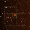 |
Fig. 1. Centaurus cluster. The image shows the four fields obtained during the observation. The field-of-view is of 1 × 1 deg2, which corresponds to 0.742 × 0.742 Mpc2, with the north pointing in the upward direction and the east in the leftward direction. The green line delimits the region analyzed in this work. |
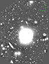 |
Fig. 2. g′ band image centered on NGC 4696 obtained at the Magellan telescope. The field-of-view (shown in green in Fig. 1) is of ∼8.795 × 11.494 arcmin2, which corresponds to ∼109 × 142 kpc2, with the north pointing the upward direction and the east in the leftward direction. The green crosses show the positions of the 5 small companions of NGC 4696 for which we calculated the models of the surface brightness distribution (Table 3). |
Observations summary.
2.2. Subtraction of the galaxy light distribution
In order to maximize the detection and perform photometry of the GC candidates, we first calculated the models of the surface brightness distribution of NGC 4696 and of other five galaxies in its proximity for each filter and subtracted them from the images. In this way the residual images show compact sources otherwise immersed in the galaxies light. The models of the surface brightness distribution were obtained using ISOFIT and CMODEL packages (Ciambur 2015) in IRAF1. These are implementations of the ELLIPSE and BMODEL tasks (Jedrzejewski 1987), which allow to calculate the model of the surface brightness distribution by fitting elliptical isophotes to the galaxy via a Fourier series expansion. The surface brightness of the isophotes is calculated as:
 (1)
(1)
where ⟨Iell⟩ is the surface brightness the isophote would have if it was a perfect ellipse, ψ is the eccentric anomaly, and An and Bn are the Fourier coefficients (Ciambur 2015).
We used ISOFIT because we find it to be more accurate than ELLIPSE in the interpolation of the isophotes in this case. In fact, it samples them using the eccentric anomaly, which results in equal length arcs on the ellipse and describes better the deviations from the elliptical form of the isophotes. In order to calculate these deviations, the program allows the user to add higher harmonics and use them as input for the CMODEL task. For the case of NGC 4696, we used the first four harmonics, which are given by default and describe the coordinates of the center of the galaxy, the ellipticity and the position angle, and we add the n = 6 and n = 8 harmonics in the g′ and i′ bands, and the n = 6 harmonic in the r′ band. We only used the even harmonics because the odd ones introduce a negligible correction in the case of a galaxy with no significant asymmetries (Ciambur 2015), such as NGC 4696. The models were calculated after masking external galaxies and point-like sources present in the field, in order to have a precise measure of the light of the galaxy under consideration. The properties of the other five galaxies analyzed, and the parameters used in ISOFIT are listed in Table 3.
Properties of the five galaxies for which the models of the surface brightness distribution were calculated.
2.3. Source detection and photometry
After the subtraction of the models from the images, we run the SExtractor package (version 2.19.5; Bertin & Arnouts 1996) to detect sources. After some experimentation, we chose a Gaussian filter, a detection threshold of 3 × σsky, a detection minimum area of 5 pixels, a background filter size of 3, and different background meshes (ranges from 4 to 24) in order to maximize the detection of point-like sources. We found 14 507 sources in common in the three filters. The magnitudes of the sources were calculated using the parameter MAG_ISO of SExtractor, which in our case has typically lower errors with respect to MAG_APER. Moreover, since we noticed that in both Harris et al. (2006) and Harris (2023) the color distribution of the GC candidates show a deep between the blue and red populations that is not evident in our analysis, we compared the color distribution obtained with MAG_ISO with that obtained with MAG_APER. However, neither the use of MAG_APER shows the deep between the red and blue populations in the color distribution, so for the following analysis we use MAG_ISO. The photometric calibration was performed using standard stars from the NOAO Source Catalog (Nidever et al. 2020). We found 3490 sources in common between ours and the NSC catalogs. For the calibration we considered only those sources for which in the NSC catalog the number of observations was > 1, and that have a stellarity index > 0.5 in order to exclude extended sources. Moreover, we visually checked the remaining 925 objects in order to exclude the ones that were located near other sources or that were too immersed in the light of the galaxy. After the inspection, we decided to use 105 sources to calibrate our sample. The rms scatter of the observed minus catalog magnitudes is of 0.02 mag. Finally, we corrected the magnitudes for Galactic extinction according to the values shown in Table 1. The magnitudes reported in this work are in the AB system.
Besides the magnitude of the sources, SExtractor allows the user to estimate the type of object analyzed with the CLASS_STAR parameter, which has values between 0 and 1 (Bertin & Arnouts 1996). In particular, objects with CLASS_STAR = 1 are stellar objects, while those with CLASS_STAR = 0 are extended objects. In order to separate GCs from galaxies, we divided the detected sources into two subsamples with CLASS_STAR > 0.5, and CLASS_STAR ≤ 0.5. The typical effective radius of GCs is reff ∼ 3 pc, which corresponds to ∼0.015 arcsec at the distance of Centaurus. This means that most of them are unresolved, so we selected sources with CLASS_STAR > 0.5, in the i′ filter, which corresponds to the image with the best seeing conditions. In this way, we found 10 970 compact (or unresolved) sources, which are shown in the color-magnitude diagram in the top panel of Fig. 3.
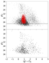 |
Fig. 3. Comparison between the color magnitude diagram of the sources and that of the background regions. Top panel: color-magnitude diagram of the 10 970 sources (black dots) selected according to their shape. The plot shows the g′0 magnitude as a function of the (g′−i′)0 color. The horizontal line at g′0 = 26.789 shows the limit applied as conservative measure in order to avoid eventual color trends due to the incompleteness of the sample. The red dots represent the sources after the selection on color and magnitudes, and the black bars are the mean errorbars in the magnitude bins used to calculate the color distributions and the positions of the blue and red peaks. Bottom panel: color-magnitude diagram of the background regions. The plot shows the g′0 magnitude as a function of the (g′−i′)0 color for the 1138 sources located in the two rectangle regions of 6 × 1 arcmin2 used to calculate the background level. |
3. Selection of globular cluster candidates
Fig. 3 shows a very large spread in color of the selected sources. In order to eliminate potential contaminators from the 10 970 compact sources sample, such as foreground and background sources, we applied a second selection criterion based on (g′−r′)0 and (r′−i′)0 colors, and on the g′0 magnitudes. In particular, we used 0.35 < (g′−r′)0 < 0.85, 0.0 < (r′−i′)0 < 0.55, and g′0 > 22.0 as described in Faifer et al. (2017). These limits were obtained in Faifer et al. (2011) for the GCSs of five early type galaxies located at a distance modulus between 29.93 ± 0.09 and 31.90 ± 0.20. Given these distances and that of NGC 4696, we can apply the same color selection since redshift effects are negligible. The color limits were obtained by Faifer et al. (2011) by considering the completeness of the GC sample and the magnitudes of Galactic globular clusters. In particular, the bright limit corresponds to MI > −12 mag, which represents the typical separation between GCs and UCDs. Moreover, as shown in Fig. 8 in Faifer et al. (2011), the limits cover the metallicity range expected for GCs. Our selection considers a somewhat larger range in color to take into account for the increasing errors going toward fainter magnitudes. Using these limits, we obtained a sample of 3973 GC candidates, whose properties are summarized in Table A.1. From Fig. 3, we can see some black dots in the same region of our selected sources. This is given by the fact that the color selection was made only on the (g′−r′)0 and (r′−i′)0 colors. Fig. 4 shows the positions of the sources with respect to the center of the host galaxy.
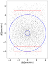 |
Fig. 4. Positions of the globular cluster candidates with respect to the center of the galaxy. The plot shows declination and right ascension of the sources, in which the center of NGC 4696 is located at (Δα, Δδ) = (0, 0). The blue circles define the borders of the annulus inside of which the azimuthal distribution of the GCs was calculated, whereas the red rectangles represent the regions where the contamination level from background objects and foreground stars was calculated. |
4. Results
4.1. Color-magnitude and color-color diagrams
At this point, the sample of GC candidates, defined using a selection on the stellarity index (CLASS_STAR > 0.5 in the i′ filter), the colors (0.35 < (g′−r′)0 < 0.85 and 0.0 < (r′−i′)0 < 0.55) and magnitude (g′0 > 22), includes 3973 sources. In the color-magnitude diagram (Fig. 3) we note that a color dependence of the limiting magnitude can be spotted as the mild trend at fainter magnitudes: blue GC candidates are more prone to be detected than red ones, within the color range defined in Sect. 3. In order to test the detection limits of our photometry, we performed the completeness test of the GC sample. In particular, we used the ADDSTAR task (Stetson 1987) in IRAF to add 200 artificial star-like objects per each magnitude considered based on the PSF estimated with DAOPHOT. The task allows the user to add point-like sources at chosen magnitude and positions, which in our case is important to recover their colors. The artificial stars were then added in the three filters at chosen positions in steps of 0.2 magnitudes, so the total number of sources added with magnitude of 16.2 ≤ g′0 ≤ 29.0 mag is 12 000. The addition of 200 objects in each step allows to get a good number statistics, but also to avoid crowding effects. Using the same SExtractor parameters as described before, we determined how many of the added stars could be recovered in the three filters. The magnitudes were then corrected according to the same zeropoint and extinction values as in the precedent analysis (Table 1). Moreover, we made sure that the artificial stars were added in the same positions in all the three filters, and that they had a color of (g′−i′)0 = 0.878 which represent the mean value of our sample. As can be seen in Fig. 5, the 50% completeness limit is reached at a magnitude g′0 = 26.889 mag, so by choosing to limit our study at g′0 ≤ 26.79 mag, where we have a 67% completeness, we are well above the 50% completeness.
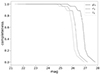 |
Fig. 5. Completeness test results. The solid, dashed and dotted lines show the completeness for the g′, r′ and i′ bands respectively. |
Despite the morphological and color selection criteria, some of the point-like sources are likely to be foreground stars or background galaxies, so an additional correction must be applied. For an upper limit estimate of the potential background contamination, we selected two rectangular regions of 6 × 1 arcmin2, located in the upper and lower parts of the field of view (see Fig. 4), where they in part overlap the circular region because the image is not fully symmetric around NGC 4696. The radius of the circular region is of 4.091 arcmin (2.4 reff), and it was chosen in order to have the largest possible symmetrical region around NGC 4696 within the observed field. We run the photometry and the completeness test on the rectangular regions using the same parameters as before. The total number of sources in the background regions is of 1138, whereas the number of sources with g′0 > 22 mag is of 526 and 530 for the upper and lower regions, respectively. The color-magnitude diagram of these sources is shown in Fig. 3. As can be seen, it looks much like the CMD of the central one, supporting the hypothesis that it is also dominated by GCs. Of the sources added with the task ADDSTAR, 16 fall inside the upper region and 15 in the lower one.
Finally, to estimate which fraction of sources in the above mentioned background fields corresponds to foreground stars in the Milky Way, we compared our results with the star counts given by the Besançon model of the Galaxy2 (Robin et al. 2003). We run the simulation for the MegaCam filters, considering a region with the same area as our background regions and with 18.0 ≤ g′0 ≤ 28.0 mag. With these values, we found 104 sources, of which only 3 are within the range of the color-magnitude cut applied to select our GC candidates (Fig. 6). From this result, we can conclude that the contribution of foreground stars to the background level is negligible. In order to have an estimation of the contribution from background galaxies we would need to go to much larger galactocentric distances. For the time being, we will then assume the background level to be negligible.
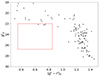 |
Fig. 6. Color-magnitude diagram of the sources in the Besançon model simulation. The plot shows the g′0 magnitude as a function of the (g′−r′)0 color, for the sources in an area equal to that used for our background fields (6 × 1 arcmin2). The red square shows the limits given by our GCs selection criteria. |
With the faint magnitude cut given by the completeness test described above, the number of GC candidates, shown by the red dots in Fig. 3, reduces to 3818. From the photometry of the GC candidates we obtained the color-magnitude diagram, and the color-color diagram and color distributions, which are shown in Figs. 7 and 8 respectively. We compared our catalog of point-like sources with the 27 compact objects, for which a membership to the Centaurus cluster was spectroscopically confirmed by Mieske et al. (2007). We found 17 sources in common, of which 12 belong to our sample of 3818 GC candidates, whereas the remaining 5 sources belong to the sample after the selection made only on the stellarity index. For comparison, Fig. 8 shows the 12 compact sources belonging to our GC candidates sample. As can be seen, the color properties of these compact objects are well described within our selection criteria.
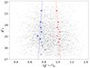 |
Fig. 7. Color-magnitude diagram of the 3818 globular cluster candidates. The plot shows the g′0 magnitude as a function of the (g′−i′)0 color. The blue and red points correspond to the peaks of the blue and red GC populations, obtained by forcing the fit of two Gaussians on each subsamples of GCs. The blue and red star symbols represent the bins for which the bimodal distribution was confirmed by the Akaike Information Criterion. The blue and red x symbols represent the peaks of the total population of GC candidates, whereas the circles represents the bins for which the Akaike Information Criterion gave a non-bimodal distribution. The blue and red lines correspond to the best linear fits for the peaks in the color distributions. |
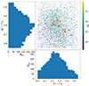 |
Fig. 8. x versus y color-color diagram of the 3818 globular cluster candidates selected according to their shape, color, and magnitude. The plot shows the (g′−r′)0 as a function of (r′−i′)0, color coded according to the g′0 magnitude. The left and bottom panels show the (g′−r′)0 and (r′−i′)0 color distributions, respectively. The red stars represent compact objects identified by Mieske et al. (2007) which were recovered in our selection. The properties of these objects are summarized in Table B.1. |
4.2. Color distribution
As indicated by Fig. 7, the (g′−i′)0 color distribution is clearly more complex than a single Gaussian. Bimodality has been found in most GCSs of giant galaxies and indeed NGC 4696 shows a distribution that could be well represented, at first glance, by two Gaussians. In order to investigate this issue, we performed the analysis of the color distribution of the GC candidates with the Gaussian Mixture Modeling of sklearn in Python (Pedregosa et al. 2011), which allows to fit multiple Gaussians to check for multimodality. From this, we find that a bimodal Gaussian, with the blue peak at (g′−i′)0 = 0.763 ± 0.004 mag and the red peak at (g′−i′)0 = 1.012 ± 0.004 mag, is preferred over a unimodal and a trimodal one, see right panel of Fig. 9. The red and blue populations were divided at the color for which the GMM fit gave an equal probability for the object of belonging to the red or blue subsamples (as described in Escudero et al. 2018). In our case the color cut of the total sample corresponds to (g′−i′)0 = 0.905 mag, which, given the transformations from Table 3 of Jordi et al. (2006), is bluer than the value found by Harris et al. (2006). To test whether two Gaussians are preferable instead of three or more Gaussians, we used the Akaike Information Criterion (AIC; Akaike 1974) implemented in astroML (VanderPlas et al. 2012), which, given the data and a certain number of components for the model, estimates the quality of the model. We performed the AIC test using a number of components from 1 to 5. As can be seen in Fig. 9 the best fit, for which the value of the AIC is minimum, is obtained for a 2 Gaussian model.
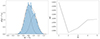 |
Fig. 9. Akaike Information Criterion test. Left panel: probability density function vs the (g′−i′)0 color. The black line represents the best fit model, the dashed lines represent the two Gaussians described by the model. The color distribution is divided in bins according to the Freedman-Diaconis rule (Freedman & Diaconis 1981). Right panel: values of the Akaike Information Criterion (AIC) as a function of the number of components in the model. |
4.3. The blue tilt
A large fraction of GCSs around external galaxies shows the so-called blue tilt in the color distribution (e.g., Forbes et al. 2010; Faifer et al. 2011; Harris et al. 2006; Mieske et al. 2005). This means that, in a bimodal color distribution, the blue peaks become redder for increasing cluster’s luminosities. In order to investigate this, we divided the GC candidates in subsamples according to their magnitudes, and making sure to have a comparable number of candidates in each bin in order to have a good number statistic. We then calculated the color distribution for each bin using the Kernel Density Estimation (KDE). This is a nonparametric method, which allows to estimate the shape of a density function, given a sample from the distribution (Karppa et al. 2021). For our analysis, we calculated the KDE using a Gaussian kernel, whose shape and size was kept fixed for each magnitude bin. Fig. 10 shows the KDE of the color distribution for each subsample with the respective number of GCs, while Fig. 11 shows the superimposition of the color distributions. As can be seen from the plots, in some of the bins the color distributions are not unimodal, but they show at least two peaks. This was confirmed by the results of the Akaike Information Criterion summarized in Table 4. In particular, the positions of the blue and red peaks are shown in Fig. 11. However, considering the errorbars of the linear fits we can not detect a significant blue tilt Fig. 7. In fact, the slope of the linear fits is consistent with zero for both the blue:
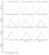 |
Fig. 10. Color distribution of the subsamples of globular clusters. The plots go from the brightest magnitude bin (top left) to the faintest magnitude bin (bottom). The legends indicate the number of GCs for the considered bin. The number of components that better fit the color distributions in each bin according to the Akaike Information Criterion are summarized in Table 4. |
 (2)
(2)
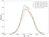 |
Fig. 11. Color distribution of the subsamples of GCs. Each curve shows the color distribution within the indicated magnitude ranges. The widths of the magnitude bins were chosen to have a comparable number of sources per range. |
and the red peaks:
 (3)
(3)
We note that in the brightest magnitude bin, although the Akaike Information Criterion points toward a unimodal color distribution (Table 4), the two calculated peaks for the bimodal case seems to fall along the linear fits for the two populations (Fig. 7). In order to test our results, we then repeated the linear fits with the addition of these two points. We note that the best fit parameters are not significantly different from the previous ones, but the addition of these two points result in a decrease in the errors of the parameters. In particular, for the blue population we have m = −0.011 ± 0.009 and q = 1.022 ± 0.215, while for the red population m = 0.013 ± 0.009 and q = 0.691 ± 0.227, where m and q are the slope and intercept of the fitted line.
Best-fit parameters for the Gaussian mixture modeling of the (g′−i′)0 color distribution of GC candidates.
4.4. Radial trends of the color distribution
In order to study eventual color gradients across the galaxy, we divided the GC sample in subsamples of radial bins, and calculated the color distribution for the (g′−i′)0, (r′−i′)0, and (g′−r′)0 colors in each bin. In particular, at r ≤ 1′ a visual inspection shows what appears to be a sample of clusters more concentrated toward a single, intermediate value of the (g′−i′)0 color (Fig. 12). The Akaike Information Criterion shows (Table 5) that for the innermost bin and the one with 1′< r ≤ 1.7′, the subsamples are better described by unimodal color distributions, with peaks of the Gaussians in both cases being at (g′−i′)0 = 0.921. However, data for r ≤ 1 arcmin should be taken with caution as the high noise associated with the galaxy body hampers a reliable detection and characterization of GCs in this region. In the three outermost bins, the color distributions appear bimodal, with both the blue and red peaks shifting toward bluer colors as we go toward larger galactocentric distances. The results are shown in Fig. 13 and in Table 5. From this analysis, the color distribution shows a trend with radius, such as it has been observed for other early type galaxies (Bassino et al. 2006). To better quantify this trend, we performed a linear fit of the blue and red peaks, as well as on the medians between the two peaks which represent the color separation between the two populations. The linear fits are shown in Fig. 12 and the best fit parameters are reported in Table 6.
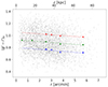 |
Fig. 12. (g′−i′)0 color versus radius plot. The black dots represent the 3818 GC candidates. The blue and red dots are the blue and red peaks of the color distributions divided into bins as explained in this section. The green dots represent the medians between the blue and red peaks. The blue, red, and green lines are the linear fit of the peaks. The blue and red stars represent the peaks of the total color distribution. The effective radius of the galaxy is reff = 1.7′, which at the distance of NGC 4696 corresponds to 21.02 kpc. |
Best-fit parameters for the Gaussian mixture modeling of the (g′−i′)0 color distribution of GC candidates divided into radial bins.
 |
Fig. 13. (g′−i′)0, (g′−r′)0, and (r′−i′)0 color distributions for the globular cluster subsamples in different radial bins. The number of sources in the different bins is NGC = 428 (blue), NGC = 634 (red), NGC = 1638 (green), NGC = 540 (black), and NGC = 578 (magenta). |
Assuming that our GC candidates are all coeval and old, to check our results, we converted the colors in metallicities, such as (Faifer et al. 2011):
![Mathematical equation: $$ \begin{aligned}{[\mathrm{Z/H}]}=3.51*(g\prime -i\prime )_0-3.91. \end{aligned} $$](/articles/aa/full_html/2024/09/aa48235-23/aa48235-23-eq15.gif) (4)
(4)
The chemical abundances [Z/H] is related to the iron abundance by Mendel et al. (2007):
![Mathematical equation: $$ \begin{aligned}{[\mathrm{Fe/H}]} = [\mathrm{Z/H}]-0.131. \end{aligned} $$](/articles/aa/full_html/2024/09/aa48235-23/aa48235-23-eq16.gif) (5)
(5)
We calculated the values of [Fe/H] for the median between the blue and red peaks (μmed in Table 5), and fitted them with
![Mathematical equation: $$ \begin{aligned}{[\mathrm{Fe/H}]}=m*\log \left(\frac{r}{r_{\rm eff}}\right)+q, \end{aligned} $$](/articles/aa/full_html/2024/09/aa48235-23/aa48235-23-eq17.gif) (6)
(6)
where r is the radius and reff is the effective radius. Our best fit parameters, m = −0.265 ± 0.077 and q = −0.899 ± 0.029, are in good agreement with those obtained in the photometric survey of GCSs in brightest cluster ellipticals by Harris (2023). We are aware that some theoretical models show the possibility that the color-metallicity relation could be nonlinear (e.g., Yoon et al. 2006), with a bimodal color distribution resulting from a unimodal metallicity distribution. However, the color-metallicity relations are only modestly nonlinear for optical color indices. Moreover, several spectroscopic studies found a bi- or even trimodal metallicity distribution for the GCSs analyzed (e.g., Caldwell & Romanowsky 2016; Villaume et al. 2019). Finally, despite the test of different types of relations, such as linear, two parts piecewise linear correlations, and continuous quadratic relations, no consensus exists yet on the color-metallicity relation (Harris 2023). Our transformations are based on Faifer et al. (2011) as described above. The positions of the peaks of the metallicity distribution inferred from these transformations are at [Fe/H]= − 1.363 ± 0.010 and [Fe/H]= − 0.488 ± 0.012, in good agreement with the values found by Harris (2023).
4.5. Spatial distribution
We calculated the radial profile of the clusters’ number surface density by counting the number of GC candidates inside circular annuli centered at the optical center of the galaxy. We chose a width of 0.167 arcmin for each annulus. Then, we calculated the density of GCs in each bin. In order to account for the spatial limits of the image, we rerun ISOFIT holding the center fixed, using a minimum semi-major axis length of 20.04 arcsec (since in our sample there are no sources inside this radius), and adopting the same bin size as indicated above. The parameter NPIX_C in the output table gives the total number of valid pixels inside a circle having radius equal to the semi-major axis calculated by the interpolation (Jedrzejewski 1987). Then the areas of the circular annuli were computed and used to estimate the average surface density at that mean radius. The calculated areas are already corrected for any geometrical incompleteness due to the position of the galaxy in the image since NPIX_C gives only the available pixels. Since the innermost bins (up to r = 0.585 arcmin) are affected by incompleteness effects due to the difficulty of identifying sources in the brightest parts of the galaxy, we decided to exclude them from the analysis. The upper limit in radius, see Fig. 4, was given by the field of view of our central pointing. Our sample is then limited to the clusters located at a distance from the center of the galaxy of 0.585 < r < 4.091 arcmin (0.344 reff < r < 2.406 reff). In this radial range, the number of GC candidates is NGC = 3083. The result is shown in Fig. 14, where the diamond symbols indicate the innermost and outermost bins excluded from the analysis, where the sharp drop in the outermost bin is given by geometric incompleteness. The remaining distribution follows a linear relation of the type
 (7)
(7)
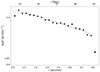 |
Fig. 14. Radial profile of the clusters’ surface density. The plot shows the density of GCs (logΣ) as a function of the distance to the center of the galaxy (r). The diamond symbols represent data not included in the regression (indicated by the solid line), in order to minimize incompleteness effects. |
in the logΣ − r plane. The parameters of the fit are reported in Table 7. The calculated areas and GC densities are reported in Table 8.
Best-fit parameters for the linear interpolation of the radial density profile of GC candidates in the logΣ − r plane.
Radial number density profile for the GC candidates.
4.6. Blue versus red population
We divided the sample into the red and blue GC populations, and calculated the radial density profiles. For the division between the blue and red clusters we adopted the fixed value of (g′−i′)0 = 0.905 mag (see Sect. 4.2). In this way, we have Nred = 1319 and Nblue = 1764. The results are shown in Fig. 15, where the diamond symbols indicate the innermost and outermost bins excluded from the analysis. As can be seen, the two populations are well described by linear relations, with different slopes. The parameters of the linear fits are reported in Table 7.
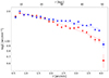 |
Fig. 15. Radial density profile for the blue and red GC populations. The plot shows the logarithm of the density of clusters (logΣ) as a function of the distance from the center of the galaxy (r) for the (g′−i′)0 ≥ 0.905 (red) and (g′−i′)0 < 0.905 (blue) subsamples. The diamonds represent the data not considered for the analysis in order to avoid incompleteness effects. |
We finally calculated the ratio between the blue and red clusters, keeping the same radial bin used for the radial density profiles. The calculated densities and ratios for each bins are reported in Table 9 and the result is shown in Fig. 16. As can be seen, the ratio of the blue to red population tends to increase going to larger galactocentric distances. This was expected since the red GCs are usually more centrally concentrated with respect to the blue ones, and it is clearly visible in Fig. 15.
Radial number density profiles for the red and blue GC populations.
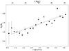 |
Fig. 16. Ratio between the blue and red populations of globular clusters. We considered radial bins of 0.167 arcmin, as in the radial density plots. The plot shows the ratio of blue to red clusters (Nblue/Nred) as a function of the distance from the center of the galaxy (r). The diamonds represent data not included in the study in order to avoid incompleteness effects in the innermost bin. The line shows the result of the linear fit to the data. |
4.7. The azimuthal distribution of the globular cluster candidates
We studied the angular distribution of the GC candidates in order to determine if they are distributed with some preferential direction, since this is an additional test to probe the interaction and merger history of NGC 4696. In particular, the comparison with the positions of the galaxies NGC 4709 and NGC 4696B (see Table 10) is important since Walker et al. (2013) outlined that the X-ray emission shows a temperature excess in the direction of NGC 4709 and a filamentary structure extending to NGC 4696B. The angular distances and directions of the two galaxies with respect to NGC 4696, calculated using Aladin3 (Bonnarel et al. 2000; Boch & Fernique 2014) by drawing a distance vector between the centers of the galaxies, are shown in Table 10. We tested the results by calculating the PA using the coordinates package in Astropy (Astropy Collaboration 2013, 2018, 2022), which given the coordinates of two objects calculates the position angle of one with respect to the other. The calculation gave similar results to those obtained with Aladin (107.1° for NGC 4709 and 284.9°) for NGC 4696B.
Parameters of the galaxies NGC 4696B and NGC 4709.
As for the radial number density profile, we limited our study to the annulus defined by 0.585 ≤ r ≤ 4.091 arcmin. With this radial selection we obtained a symmetrical region around the galaxy. The angular distribution of the total, red and blue distributions is shown in Fig. 17, where all the samples are divided in angular bins of θ = 30°. The angular positions of the GCs are measured eastward starting from the north axis.
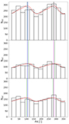 |
Fig. 17. Azimuthal distribution of 3083 globular cluster candidates. The plots show the number of clusters (NGC) as a function of the position angle (PA), divided in angular bins of 30°. The red line represents the interpolation with the function described in Eq. (8) to the data, the blue and magenta lines represent the angular positions of NGC 4709 and NGC 4696B respectively, the green lines represent the position angle of the peaks, and the dashed black lines represent the fit with Eq. (9). The different panels show the distributions of the total (top panel), red (middle panel), and blue (lower panel) GC samples. |
As can be seen, the distributions appear to have a sinusoidal shape, so we used optimize package of SciPy (Virtanen et al. 2020) to determine the best fit to the data. In particular, we noticed that the azimuthal distribution looks more complex than a simple sinusoidal. In order to take into account for the asymmetric shape of the distribution, we fit it with the function
![Mathematical equation: $$ \begin{aligned} y=a+b*\sin \left[\frac{m*\pi *(x-c)}{180}-0.5*\sin \left(\frac{m*\pi (x-c)}{180}\right)\right], \end{aligned} $$](/articles/aa/full_html/2024/09/aa48235-23/aa48235-23-eq23.gif) (8)
(8)
and we compared the results with a symmetrical sinusoidal function given by
![Mathematical equation: $$ \begin{aligned} y=a+b*\sin \left[\frac{2\pi *(x-c)}{180}\right], \end{aligned} $$](/articles/aa/full_html/2024/09/aa48235-23/aa48235-23-eq24.gif) (9)
(9)
where y is the number of clusters, x is the position angle, a is the vertical shift of the function, b is the amplitude, and c is the phase shift. After some careful attempts of fitting, we decided to fix the value of m. The best fit parameters and the positions of the two peaks of the sinusoidal fit for the total, red and blue distributions are reported in Table 11. It is important to note that the peaks found with the fit of the asymmetrical sinusoidal are much closer to the directions of NGC 4709 and NGC 4696B with respect to those obtained with the simple sinusoidal fit.
Azimuthal distribution of the GC candidates.
The sinusoidal shape of the GC counts is typical of an elliptical distribution of the GCS. In order to calculate the ellipticity, we performed the 2D Kernel Density Estimation of sklearn.neighbors (Pedregosa et al. 2011) to create a grid of the sample locations using the physical positions of the GC candidates in the image, and used the results to fit a Bivariate Gaussian Distribution using a routine in astroML (VanderPlas et al. 2012). The outputs of this routine are the position of the center of the ellipse, the sigmas of the two Gaussians which can be used as major and minor axis to calculate the ellipticity, and the position angle. The results of the routine within a 68% confidence interval are shown in Table 12.
Shape of the GCS.
The results of the fit are shown in Fig. 17 for the total, red and blue distributions. As can be seen, all distributions appear to be sinusoidal, with the peaks positions (green dashed lines) equal or extremely close to the directions of the galaxies NGC 4709 and NGC 4696B, represented by the blue and magenta lines.
4.8. Comparison with NGC 4696 profile
In order to have a preliminary idea of the radial surface brightness profile of NGC 4696, we rerun ISOFIT with the same parameters as before but keeping the position of the galaxy’s center fixed. This allows to highlight eventual asymmetries in the isophotes’ shapes. Through the Fourier coefficients a3, a4, b3, and b4, we can quantify the deviations from the elliptical shape of the isophotes (Ciambur 2015). The b4 coefficient results particularly important: positive values describe a disky isophote, whereas negative values describe a boxy isophote. The surface brightness profiles along the major axis, the position angles, ellipticities, and the values of the Fourier coefficients are shown in Fig. D.1. Our profiles are spatially limited to a galactocentric radius of ∼2.4 arcmin, so they do not reach the outermost regions of the halo. From these preliminary results, we can see some strong fluctuations in the values of the position angle and ellipticity of NGC 4696, from the inner to the outer regions. This could be due to the presence of the dust lanes in the central regions of the galaxy, and to past interactions with other galaxies in the cluster. Moreover, we see that there is a change in the value of the parameter b4, which goes from negative values in the inner regions to positive values in the outer regions. This suggests that some outer isophotes have a disky shape, a feature that will be further analyze in a future paper (Federle et al., in prep.). Comparing the values with those found for the shape of the GCS (Table 12), we can see that NGC 4696 appear to have a lower ellipticity and position angle with respect to the total, red and blue GCSs. In particular, we calculated the mean value for the ellipticity and its standard deviation in a sample of 10 points around the half-light radius of NGC 4696, which, from our spatially limited analysis, is inferred to be located at a radius of r ∼ 0.45 arcmin. The ellipticity of the galaxy results of e = 0.135 ± 0.007, which is lower than the values of  ,
,  , and
, and  and found for the total, red and blue GCSs. These differences point toward a disturbed GCS, with a shape that was influenced by the past interactions between NGC 4696 and the other galaxies in the Centaurus cluster. In Figs. D.2–D.6 we show the preliminary results for the radial surface brightness profiled of the other 5 galaxies that were subtracted from the images.
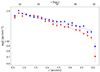 |
Fig. 18. Radial number density profiles for the blue and red GC populations, in the case of a variable (g′−i′)0 color separation between the blue and red GC populations. The plot show the logarithm of the density of clusters (logΣ) as a function of the galactocentric distance (r), for the blue and red populations defined according to Eqs. (10) and (11). The diamond symbols show the innermost and outermost bins that were not included in the fit, whereas the lines show the best linear fits. |
Linear interpolation of the radial density profile of the GC candidates.
5. Fixed versus variable color cut
As explained in Sect. 4.2, the color distribution shows a trend with radius, with the peaks of both the blue and red populations becoming bluer as we go toward larger galactocentric distances. Moreover, as shown in Table 7 in the two inner radial bins the GC population is better described by a unimodal color distribution, with peaks at (g′−i′)0 = 0.921 mag, whereas in the outer bins the distribution is clearly bimodal. In order to take into account for this radial trend, we reperformed the analysis of the radial number density profile and of the azimuthal distribution using a variable color limit to separate the blue and red GC populations. In particular, we defined as blue GCs those for which:
 (10)
(10)
and as red GCs those for which:
 (11)
(11)
where r is the radius, and the numerical values are those found by performing the linear fit on the median of the peaks in the different radial bins (the fit is shown by the green line in Fig. 12). With this definition, we obtained a number of Nred = 1393 and Nblue = 1690 for the red and blue GC populations, respectively. We then divided the two samples in radial bins of r = 0.167 arcmin, as in the previous analysis, and calculated the number density of GCs in each annulus. The results are shown in Fig. 18 and the best fit parameters are in Table 13.
Azimuthal distribution in the variable color cut case.
Shape of the GCS in the variable color cut case.
Finally, we divided the two samples in bins of 30° to study the azimuthal distribution, and perform a sinusoidal fit as explained in Sect. 4.6. The best fit parameters are reported in Table 14. In order to calculate the parameters of the red and blue GCSs, we used again the output of the 2D Kernel Density Estimation to fit a Bivariate Gaussian Distribution. The positions of the center of the systems, the position angles, minor and major axis, and ellipticities are reported in Table 15. As can be seen, the choice of a variable (g′−i′)0 value for the division between the red and blue populations results in a steeper relation for the blue radial number density profile, whereas the red one becomes less steep. Moreover, the peaks of both the red and blue populations are almost identical to what we found using a fixed color separation between the blue and red populations.
6. GC luminosity function and specific frequency
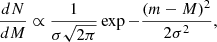
The globular cluster luminosity function (GCLF) is an important tool to determine the richness of a GC system. Furthermore, its turnover magnitude is used as a distance estimator to its host galaxy (e.g., Rejkuba 2012). It is defined as:
 (12)
(12)
where dN is the number of GCs in the magnitude bin dm, m and M are the apparent and absolute Turnover magnitudes, and σ is the width of the Gaussian distribution.
In this section we estimate the distance to NGC 4696 from the GCLF and based on that distance, determine the specific frequency SN of the GCS. SN is related to the total number of GCs and to the luminosity of the host galaxy in the V band in units of MV = −15, and it is given by Harris & van den Bergh (1981):
 (13)
(13)
where NGC is the total number of GCs and MV is the absolute magnitude of the host galaxy. It has been shown that the specific frequency depends on galaxy type and luminosity, with the highest specific frequencies occurring in low-mass dwarf galaxies and in giant ellipticals in galaxy clusters, where it reaches values ∼10 for MV < −20 mag (Peng et al. 2008; Georgiev et al. 2010).
The artificial stars experiment (Sect. 4.1) showed that there is a difference between the input magnitudes and those recovered by SExtractor, that increases going toward the fainter magnitudes. In Fig. E.1, the difference between the input and output magnitudes in the i′ band is shown as a function of the input magnitude corrected for the zeropoint and extinction coefficient. The dots represent the mean of the difference for the artificial stars recovered for a certain input magnitude. This was used to correct the magnitudes for the calculation of the luminosity function.
For the GC selection in the previous sections, we applied two simultaneous color cuts: 0.35 < (g′−r′)0 < 0.85 and 0.0 < (r′−i′)0 < 0.55, following Faifer et al. (2017). This selection ensured a clean sample. At the same time, as can be seen from Fig. 19, this simultaneous color cut reduces the number of selected GCs at faint magnitudes g′0 ≳ 25.5 mag, compared to a sample where only (g′−i′)0 color selection would be done. The photometric errors at these fainter magnitudes broaden the color distribution.
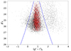 |
Fig. 19. Color-magnitude diagram of the GC candidates, zooming into the plot shown in Fig. 3. The black dots represent the full sample of point-like sources in our field. The red dots are the 3818 GC candidates defined by the two-color and magnitude selection applied for the analysis in previous sections. The blue lines represent the more inclusive single color (g′−i′)0 selection that we adopt for the analysis of the GCLF, see text for details. This corresponding sample yields 6755 candidates for the calculation of the GCLF. |
For the analysis of the total number of GCs in the GCLF, we therefore adopt a more inclusive GC selection than the two-color selection by Faifer et al. (2017). We apply a single color selection in (g′−i′)0 only, and broaden the selection window as a function of magnitude according to the photometric uncertainties as determined from the artificial star experiments. The resulting selection window is indicated in Fig. 19 and is defined by the following function:
 (14)
(14)
where a = 3.619 ± 0.165, b = 0.051 ± 0.002, and c = −1.869 ± 0.165. Finally, we considered only sources with magnitude g′0 > 22.0 mag, and in the region closer to NGC 4696 (r ≤ 4.091 arcmin). This leaves us with a sample of 6755 GCs.
To derive the GC luminosity function, we calculated the number of clusters in bins of 0.2 mag and corrected them according to the completeness values as determined from artificial star experiments (Fig. 5). We note that those completeness tests were done assuming the average color of the GC sample, and requiring that a source be detected in all three filters. We did not apply an additional two-color selection of the detected sources. This means that those completeness numbers can be applied to the more inclusive sample constructed in this section.
We assumed the absolute turnover magnitude in the three bands to be Mg′ = −7.2 mag, Mr′ = −7.56 mag, and Mi′ = −7.82 mag (Jordán et al. 2007). The GCLF assumes the form of a Gaussian distribution, such as:
![Mathematical equation: $$ \begin{aligned} N_{\rm GC}=A\exp {\left[-\frac{1}{2}\left(\frac{x-\mu }{\sigma }\right)^2\right]}, \end{aligned} $$](/articles/aa/full_html/2024/09/aa48235-23/aa48235-23-eq108.gif) (15)
(15)
where A is the amplitude, x is the magnitude in the considered band, μ is the mean that will be used as the turnover magnitude, and σ is the standard deviation. The result of the Gaussian fit in the g′, r′ and i′ bands are shown in Fig. 20, whereas the magnitudes up to which the fit was performed, the best fit parameters and the calculated distances are reported in Table 16. The derived distances in the three bands agree with each other within their error bars. The error weighted mean distance between the three bands is 38.36 ± 2.49 Mpc. This is consistent with the distance of 42.5 ± 3.2 Mpc from Mieske et al. (2005).
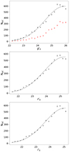 |
Fig. 20. Globular cluster luminosity function. Top panel: GCLF in the g′ band, where the black points represent the number of clusters corrected for the completeness fraction divided in bins of 0.2 mag, the solid line represent the best fit Gaussian. The red diamonds represent the number of sources in the two rectangular regions considered for the background, corrected by the completeness fraction and normalized by the area. Middle and Bottom panels: GCLF in the r′ and i′ band, where the points represent the number of clusters corrected for the completeness fraction divided in bins of 0.2 mag, and the blue lines correspond to the magnitude of the completeness limit. |
Best-fit parameters for the GCLF.
As explained in Sect. 4.2, we did not apply any statistical correction to our sample for foreground stars since the Besançon Model of the Galaxy shows that the contribution of foreground stars in this region is negligible. As a further sanity check, we calculated the luminosity function in two rectangular regions with an area of 6 arcmin2 each, located in the upper and lower part of the image well outside the region defined by the model of the surface brightness distribution of the galaxy. We applied the same inclusive color selection defined in Fig. 19 for this comparison field. Concerning background galaxies, we expect the contribution to the background level to be negligible. In fact, as shown in Fig. 3 in Fensch et al. (2014), most of the background contributes in the bluest part of the color distribution, which was in part excluded by the considered color selection. Blue background sources could still affect our sample, so in order to check how they would affect the results we made a more strict (g′−i′)0 color selection, considering a broadening in color corresponding to 75% of the previous one. This excludes more sources at the blue end of the luminosity function. The number of GCs decreases of 2.26%, which results in a nonsignificant change in the values of the distance and specific frequency.
As a final check, we compared the luminosity function in this comparison field with that for the GC candidates of NGC 4696 (top panel of Fig. 20). The counts in the comparison field are renormalized to correspond to the same total area as the NGC 4696 sample. The fit of the luminosity function to the sources in the comparison field shows a fainter turnover magnitude (g′0 = 26.32 ± 0.22) with respect to the central region of NGC 4696 (g′0 = 25.88 ± 0.14). In order to quantify the potential effect of faint background sources on top of the GCLF in the comparison field, we forced the fit of the luminosity function with the same μ and σ used for the GC candidates but with free A on the background point-like sources, and excluding the three faintest bins. This showed an excess of background sources in the three lower magnitude bins, corresponding to about 10% of the number counts in the background field. Given the scaling in source density between the background field and the GC candidate field, this implies about 6% contamination by background sources for the GC candidate sample. Based on this, a correction will be applied to the calculation of the specific frequency. In a future work we plan to improve the background level estimation by adding NUV and/or NIR photometry.
The total number of clusters is given by
 (16)
(16)
where A and σ are the amplitude and the standard deviation of the GCLF, respectively, and the bin size = 0.2 mag. The total number of sources is obtained by integrating the fitted GCLF, resulting in NGC, g′ = 10069, NGC, r′ = 9948, NGC, i′ = 9741, respectively. We adopt the mean of those three numbers NGC = 9919. As apparent magnitude for NGC 4696 we assume the value of mV = 10.05, found by Misgeld et al. (2009) via the curve of growth analysis on VLT images with a field of view smaller than that considered in this work. Assuming a distance modulus of (m − M) = 32.92 (38.36 Mpc as determined previously), we found MV, NGC 4696 = −22.87 mag. With these values, we obtain a lower limit for the specific frequency of SN = 7.1 ± 0.9. Correcting this for the estimated 6% background contamination, the final value becomes SN = 6.8 ± 0.9. This agrees within the errorbars with the value of 7.3 ± 1.5 found in Mieske et al. (2005), and is also in reasonable agreement with the values obtained for other giant ellipticals (Peng et al. 2008; Georgiev et al. 2010; Harris et al. 2013), if slightly at the lower end.
7. Discussion and conclusions
We presented the analysis of the GCS of the giant elliptical NGC 4696. The measurements are based on deep Magellan 6.5m/MegaCam (g′, r′, i′) photometry. The following results were obtained:
-
Applying a two color selection we identify a total of 3818 GC candidates. The GC system has a bimodal color distribution, with peaks at (g′−i′)0 = 0.763 mag and (g′−i′)0 = 1.012 mag, with the blue and red populations divided at (g′−i′)0 = 0.905 mag.
-
It is worth noticing that the blue and red peaks of the distribution appear well separated only in half of the magnitude bins analyzed. In particular, we notice that in the brightest bin the distribution becomes unimodal as in some of the galaxies analyzed by Faifer et al. (2011). It is also interesting to notice that, as shown in Table 4, in the faintest magnitude bins the color distribution changes as well from a bimodal to a unimodal or trimodal shape. In the last considered bin, the number of GC candidates is much lower than in the other ones. As a test in order to have a better number statistic, we joined the two faintest magnitude bins (g′0 > 25.944 mag). Here we have a total of 616 sources. We performed the GMM fit and the AIC test. We found that in this subsample a trimodal distribution is preferable to both the unimodal and bimodal distributions. In this case, we found Bootstrap (DD) = 3.53 ± 0.64 and that the three Gaussians peak at (g′−i′)0 = 0.633 ± 0.011, (g′−i′)0 = 0.858 ± 0.005, and (g′−i′)0 = 1.086 ± 0.008, suggesting then the presence of an intermediate GC population.
-
The color distribution of the GC samples, divided according to the galaxy’s effective radius, shows a trend with galactocentric radius. In particular, in the outer bins the color distribution present a bimodal shape, whereas the distribution in the inner bin is unimodal, with peaks somewhere in between those of the bimodal cases. This suggests the presence of an intermediate GC population, and could indicate a different origin for these GCs, like accretion of dwarf galaxies and merging events such as was found in previous studies of GCS around early type galaxies (Caso et al. 2017).
-
Assuming coeval and old ages of all GCs, we calculated the values of [Fe/H] using the conversions described in Faifer et al. (2011), and fitted the corresponding values of [Fe/H] for the median peaks with log(r/reff). We found that the best fit parameters for the linear interpolation are in good agreement with those found by Harris (2023). Moreover, the metallicity distribution appears bimodal with peaks at [Fe/H]= − 1.363 ± 0.010 and [Fe/H]= − 0.488 ± 0.012.
-
The radial density profile, limited to a radius of 0.585 ≤ r ≤ 4.091 arcmin in order to avoid incompleteness effects in the innermost and outermost regions of the galaxy, for the blue and red GC samples (Fig. 15) shows different slopes. The plots show that there is a significant difference between the two profiles in the outer regions of the galaxy, with the number of blue clusters being a factor of 2 higher than the red ones, whereas in the inner parts the numbers are very similar.
-
The azimuthal distributions for the total, red and blue populations of GC candidates, limited to a radius 0.585 < r < 4.091 arcmin (0.344 reff < r < 2.406 reff), are well fitted by an asymmetrical sinusoidal distribution. In particular, we found that the peaks of the distributions are close or almost perfectly aligned to the angular positions of the galaxies NGC 4709 and NGC 4696B. Moreover, we found that the ellipticity of the GCS is different with respect to that of the host galaxy. This indicates that the interactions between NGC 4696 and these two galaxies played a role in shaping the GCS under consideration. Moreover, these results agree with the merger/interaction history outlined by previous works on the hot X-ray gas, such as the identification of a filamentary structure connecting NGC 4696 with NGC 4696B and a metallicity excess around NGC 4709 by Walker et al. (2013), and an asymmetric temperature variation with the hottest region coinciding with NGC 4709 by Churazov et al. (1999).
-
Since we notice that the color distribution shows a trend with radius, we decided to recalculate the radial density profiles and the azimuthal distributions using a variable (g′−i′)0 color separation between the blue and red GC populations. In particular, we separated the two using the linear fit on the median between the blue and red peaks (given by (g′−i′)0 = −0.01556 * r + 0.92990). In this case, the radial density profile of the blue population becomes steeper than in the case of a constant color separation, and the differences between the two profiles become negligible in the inner regions and much less pronounced in the outer regions. In a future work, we aim at expanding our sample to further investigate the importance of the choice of the color separation between the blue and red GC populations.
-
We calculated the GCLF in the three filters, and used it for our own estimation of the distance of NGC 4696, as well as the specific frequency. As can be seen from Table 16, the distances estimated in the different filters are consistent within the errors. Moreover, our results are consistent with the measurement of the distance of the Centaurus cluster obtained with both the GCLF and the surface brightness fluctuation method by Mieske et al. (2005). Finally, we used the peak of the GCLF to estimate the total number of GCs in NGC 4696, assuming that the luminosity function is described by a symmetric Gaussian. We then used the number of clusters to estimate the specific frequency of the system, and corrected it for the 6% contamination by background galaxies estimated from the comparison between the luminosity function of the GC candidates and that of the sources in the two rectangular regions defined in Sect. 3. The specific frequency resulted of SN ∼ 6.8. This value is to consider a lower limit since the study is limited to a radius of 4.091 arcmin, so we are missing the GC population at the highest galactocentric distances. However, it is well within the range for giant ellipticals in galaxy clusters, and agrees with previous calculations (Mieske et al. 2005).
As a final note, the next step in the analysis will be the spectroscopic follow-up of our GC candidates. The addition of spectroscopic data to our study will be fundamental to confirm their affiliation to NGC 4696. This will allow also to investigate with more precision the interaction history of the host galaxy, and to understand the history of the cluster itself, as was highlight in other analysis such as that of the Virgo (Durrell et al. 2014), Coma (Madrid et al. 2018) and the Fornax (Chaturvedi et al. 2022) clusters, and Abell 1689 (Alamo-Martínez et al. 2013). Moreover, we will add the other field to the analysis, starting with that containing NGC 4709. This will allow us to investigate its GCS, as well as the GCs between this galaxy and NGC 4696, in order to determine the role of the interactions in shaping the GCSs of these two galaxies.
Data availability
All tables are available electronically from the author upon request. The MegaCam images are accessible through the CADC image archive.
The full catalog of GC candidates (Table A.1) is available at the CDS via anonymous ftp to cdsarc.cds.unistra.fr (130.79.128.5) or via https://cdsarc.cds.unistra.fr/viz-bin/cat/J/A+A/689/A342
IRAF is distributed by the National Optical Astronomy Observatory (NOAO), directed by the Association of University for Research in Astronomy (AURA) together with the National Science Foundation (NSF). It is available in https://iraf.noirlab.edu/
Available in: https://model.obs-besancon.fr
Available in https://aladin.u-strasbg.fr/aladin.gml
Acknowledgments
S.F. and M.G. gratefully acknowledge support by Fondecyt Project N° 1220724. This research has made use of the NASA/IPAC Extragalactic Database (NED), which is funded by the National Aeronautics and Space Administration and operated by the California Institute of Technology.
References
- Akaike, H. 1974, IEEE Trans. Autom. Control, 19, 716 [Google Scholar]
- Alamo-Martínez, K. A., Blakeslee, J. P., Jee, M. J., et al. 2013, ApJ, 775, 20 [CrossRef] [Google Scholar]
- Astropy Collaboration (Robitaille, T. P., et al.) 2013, A&A, 558, A33 [NASA ADS] [CrossRef] [EDP Sciences] [Google Scholar]
- Astropy Collaboration (Price-Whelan, A. M., et al.) 2018, AJ, 156, 123 [Google Scholar]
- Astropy Collaboration (Price-Whelan, A. M., et al.) 2022, ApJ, 935, 167 [NASA ADS] [CrossRef] [Google Scholar]
- Bassino, L. P., Faifer, F. R., Forte, J. C., et al. 2006, A&A, 451, 789 [NASA ADS] [CrossRef] [EDP Sciences] [Google Scholar]
- Beasley, M. A. 2020, ArXiv e-prints [arXiv:2003.04093] [Google Scholar]
- Beasley, M. A., Trujillo, I., Leaman, R., et al. 2018, Nature, 555, 483 [NASA ADS] [CrossRef] [Google Scholar]
- Bertin, E., & Arnouts, S. 1996, A&AS, 117, 393 [NASA ADS] [CrossRef] [EDP Sciences] [Google Scholar]
- Bertin, E., Mellier, Y., Radovich, M., et al. 2002, ASP Conf. Ser., 281, 228 [Google Scholar]
- Binney, J., & Wong, L. K. 2017, MNRAS, 467, 2446 [NASA ADS] [Google Scholar]
- Boch, T., & Fernique, P. 2014, ASP Conf. Ser., 485, 277 [Google Scholar]
- Bonnarel, F., Fernique, P., Bienaymé, O., et al. 2000, A&AS, 143, 33 [NASA ADS] [CrossRef] [EDP Sciences] [Google Scholar]
- Caldwell, N., & Romanowsky, A. J. 2016, ApJ, 824, 42 [NASA ADS] [CrossRef] [Google Scholar]
- Caso, J. P., Bassino, L. P., & Gómez, M. 2017, MNRAS, 470, 3227 [NASA ADS] [CrossRef] [Google Scholar]
- Chaturvedi, A., Hilker, M., Cantiello, M., et al. 2022, A&A, 657, A93 [NASA ADS] [CrossRef] [EDP Sciences] [Google Scholar]
- Churazov, E., Gilfanov, M., Forman, W., et al. 1999, ApJ, 520, 105 [CrossRef] [Google Scholar]
- Ciambur, B. C. 2015, ApJ, 810, 120 [NASA ADS] [CrossRef] [Google Scholar]
- Côté, P., Marzke, R. O., & West, M. J. 1998, ApJ, 501, 554 [Google Scholar]
- de Vaucouleurs, G., de Vaucouleurs, A., Corwin, H. G., et al. 1991, Third Reference Catalogue of Bright Galaxies (New York: Springer) [Google Scholar]
- Dolfi, A., Forbes, D. A., Couch, W. J., et al. 2021, MNRAS, 504, 4923 [NASA ADS] [CrossRef] [Google Scholar]
- Drinkwater, M. J., Jones, J. B., Gregg, M. D., et al. 2000, PASA, 17, 227 [NASA ADS] [CrossRef] [Google Scholar]
- Durrell, P. R., Côté, P., Peng, E. W., et al. 2014, ApJ, 794, 103 [NASA ADS] [CrossRef] [Google Scholar]
- Escudero, C. G., Faifer, F. R., Smith Castelli, A. V., et al. 2018, MNRAS, 474, 4302 [NASA ADS] [CrossRef] [Google Scholar]
- Escudero, C. G., Cortesi, A., Faifer, F. R., et al. 2022, MNRAS, 511, 393 [NASA ADS] [CrossRef] [Google Scholar]
- Faifer, F. R., Forte, J. C., Norris, M. A., et al. 2011, MNRAS, 416, 155 [NASA ADS] [Google Scholar]
- Faifer, F. R., Escudero, C. G., Scalia, M. C., et al. 2017, A&A, 599, L8 [NASA ADS] [CrossRef] [EDP Sciences] [Google Scholar]
- Farrell, S. A., Webb, N. A., Barret, D., et al. 2009, Nature, 460, 73 [CrossRef] [Google Scholar]
- Fensch, J., Mieske, S., Müller-Seidlitz, J., et al. 2014, A&A, 567, A105 [NASA ADS] [CrossRef] [EDP Sciences] [Google Scholar]
- Forbes, D. A., Spitler, L. R., Harris, W. E., et al. 2010, MNRAS, 403, 429 [CrossRef] [Google Scholar]
- Freedman, D., & Diaconis, P. 1981, Prob. Theory Relat. Fields, 57, 453 [Google Scholar]
- Georgiev, I. Y., Puzia, T. H., Goudfrooij, P., et al. 2010, MNRAS, 406, 1967 [Google Scholar]
- Gnedin, O. Y. 2003, ApJ, 582, 141 [Google Scholar]
- Harris, W. E. 1991, ARA&A, 29, 543 [Google Scholar]
- Harris, W. E. 2010, ArXiv e-prints [arXiv:1012.3224] [Google Scholar]
- Harris, W. E. 2023, ApJS, 265, 9 [CrossRef] [Google Scholar]
- Harris, W. E., & van den Bergh, S. 1981, AJ, 86, 1627 [NASA ADS] [CrossRef] [Google Scholar]
- Harris, W. E., Whitmore, B. C., Karakla, D., et al. 2006, ApJ, 636, 90 [NASA ADS] [CrossRef] [Google Scholar]
- Harris, W. E., Harris, G. L. H., & Alessi, M. 2013, ApJ, 772, 82 [Google Scholar]
- Hilker, M. 2009, Rev. Mod. Astron., 21, 199 [NASA ADS] [Google Scholar]
- Hilker, M., Infante, L., Vieira, G., et al. 1999, A&AS, 134, 75 [NASA ADS] [CrossRef] [EDP Sciences] [Google Scholar]
- Ishchenko, M., Sobolenko, M., Berczik, P., et al. 2023, A&A, 673, A152 [NASA ADS] [CrossRef] [EDP Sciences] [Google Scholar]
- Jarrett, T. H., Chester, T., Cutri, R., et al. 2003, AJ, 125, 525 [NASA ADS] [CrossRef] [Google Scholar]
- Jedrzejewski, R. I. 1987, MNRAS, 226, 747 [Google Scholar]
- Jordán, A., McLaughlin, D. E., Côté, P., et al. 2007, ApJS, 171, 101 [CrossRef] [Google Scholar]
- Jordi, K., Grebel, E. K., & Ammon, K. 2006, A&A, 460, 339 [NASA ADS] [CrossRef] [EDP Sciences] [Google Scholar]
- Karppa, M., Aumüller, M., & Pagh, R. 2021, ArXiv e-prints [arXiv:2107.02736] [Google Scholar]
- Kaviraj, S., Crockett, R. M., Silk, K., et al. 2012a, IAU Symp., 284, 460 [NASA ADS] [Google Scholar]
- Kaviraj, S., Crockett, R. M., Whitmore, B. C., et al. 2012b, MNRAS, 422, L96 [CrossRef] [Google Scholar]
- Lucey, J. R., Currie, M. J., & Dickens, R. J. 1986, MNRAS, 221, 453 [NASA ADS] [CrossRef] [Google Scholar]
- Madrid, J. P., O’Neill, C. R., Gagliano, A. T., et al. 2018, ApJ, 867, 144 [NASA ADS] [CrossRef] [Google Scholar]
- McLeod, B., Geary, J., Ordway, M., et al. 2006, Astrophys. Space Sci. Lib., 336, 337 [NASA ADS] [Google Scholar]
- McLeod, B., Geary, J., & Conroy, M. 2015, PASP, 127, 366 [NASA ADS] [CrossRef] [Google Scholar]
- Mendel, J. T., Proctor, R. N., & Forbes, D. A. 2007, MNRAS, 379, 1618 [NASA ADS] [CrossRef] [Google Scholar]
- Mieske, S., Hilker, M., & Infante, L. 2005, A&A, 438, 103 [NASA ADS] [CrossRef] [EDP Sciences] [Google Scholar]
- Mieske, S., Hilker, M., Jordán, A., et al. 2007, A&A, 472, 111 [NASA ADS] [CrossRef] [EDP Sciences] [Google Scholar]
- Mihos, J. C. 2004, Clusters of Galaxies: Probes of Cosmological Structure and Galaxy Evolution (Cambridge: Cambridge University Press) [Google Scholar]
- Minniti, D., Palma, T., & Ciariá, J. J. 2021, Boletin de la Asociacion Argentina de Astronomia La Plata Argentina, 62, 107 [NASA ADS] [Google Scholar]
- Misgeld, I., Hilker, M., & Mieske, S. 2009, A&A, 496, 683 [NASA ADS] [CrossRef] [EDP Sciences] [Google Scholar]
- Nidever, D. L., Dey, A., Fasbender, K., et al. 2020, ApJ, 161, 192 [Google Scholar]
- Pedregosa, F., Varoquaux, G., Gramfort, A., et al. 2011, J. Mach. Learn. Res., 12, 2825 [Google Scholar]
- Peng, E. W., Jordán, A., Côté, P., et al. 2008, ApJ, 681, 197 [NASA ADS] [CrossRef] [Google Scholar]
- Proctor, R. N., Forbes, D. A., Romanowsky, A. J., et al. 2009, MNRAS, 368, 91 [NASA ADS] [CrossRef] [Google Scholar]
- Puzia, T. H., Zepf, S. E., Kissler-Patig, M., et al. 2002, A&A, 391, 453 [NASA ADS] [CrossRef] [EDP Sciences] [Google Scholar]
- Racine, R. 1968, J. R. Astron. Soc. Can., 62, 367 [NASA ADS] [Google Scholar]
- Reina-Campos, M., Trujillo-Gomez, S., Deason, A. J., et al. 2022, MNRAS, 513, 3925 [NASA ADS] [CrossRef] [Google Scholar]
- Reina-Campos, M., Trujillo-Gomez, S., Pfeffer, J. L., et al. 2023, MNRAS, 521, 6368 [NASA ADS] [CrossRef] [Google Scholar]
- Rejkuba, M. 2012, Ap&SS, 341, 195 [Google Scholar]
- Renaud, F., Agertz, O., & Gieles, M. 2017, MNRAS, 465, 3622 [NASA ADS] [CrossRef] [Google Scholar]
- Robin, A. C., Reylé, C., Derrière, S., & Picaud, S. 2003, A&A, 409, 523 [NASA ADS] [CrossRef] [EDP Sciences] [Google Scholar]
- Schlafly, E. F., & Finkbeiner, D. P. 2011, ApJ, 737, 103 [Google Scholar]
- Sesto, L. A., Faifer, F. R., & Forte, J. C. 2016, MNRAS, 461, 4260 [NASA ADS] [CrossRef] [Google Scholar]
- Stein, P., Jerjen, H., & Federspiel, M. 1997, A&A, 327, 952 [NASA ADS] [Google Scholar]
- Stetson, P. B. 1987, PASP, 99, 191 [Google Scholar]
- Strader, J., Brodie, J. P., Spitler, L., et al. 2006, ApJ, 132, 2333 [Google Scholar]
- Usher, C., Pfeffer, J., Bastian, N., et al. 2018, MNRAS, 480, 3279 [NASA ADS] [CrossRef] [Google Scholar]
- VanderPlas, J., Connolly, A. J., Ivezic, Z., et al. 2012, 2012 Conference on Intelligent Data Understanding (IEEE) [Google Scholar]
- Villaume, A., Romanowsky, A. J., Brodie, J., et al. 2019, ApJ, 879, 45 [NASA ADS] [CrossRef] [Google Scholar]
- Virtanen, P., Gommers, R., Burovski, E., et al. 2020, https://doi.org/10.5281/zenodo.4100507 [Google Scholar]
- Walker, S. A., Fabian, A. C., & Sanders, J. S. 2013, MNRAS, 435, 3221 [NASA ADS] [CrossRef] [Google Scholar]
- Yoon, S. J., Lee, S. Y., Yi, S., et al. 2006, Science, 311, 1129 [CrossRef] [Google Scholar]
Appendix A: Catalog of the globular cluster candidates
Properties of the globular cluster candidates of the galaxy NGC 4696.
Appendix B: Sources from previous catalogs
Properties of the candidates in our sample for which Mieske et al. (2007) confirmed the membership to the Centaurus cluster.
Appendix C: Exposure map
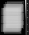 |
Fig. C.1. Exposure map in the r′ band of the region of the Centaurus cluster analyzed in this work. The colorbar shows the number of participating individual exposures in log scale. |
Appendix D: The galaxies radial surface brightness profiles
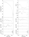 |
Fig. D.1. Radial surface brightness profile along the major axis for NGC 4696. The panels show the trend of the surface brightness (μ), the position angle (PA), the ellipticity (e), the center (x0,y0), and the Fourier coefficients a3, a4, b3, and b4 as a function of the logarithm of the semi major axis (a). The plots were obtained through the interpolation of ISOFIT on the image in the i′ band. |
Appendix E: Comparison between input and output magnitudes for the artificial stars experiment
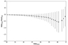 |
Fig. E.1. Comparison between the input and output magnitudes for the artificial stars’ experiment in the i′ band. The dots the means of the difference between the input and output magnitudes (MAGadd − MAGiso), whereas the errorbars are their RMS. |
All Tables
Properties of the five galaxies for which the models of the surface brightness distribution were calculated.
Best-fit parameters for the Gaussian mixture modeling of the (g′−i′)0 color distribution of GC candidates.
Best-fit parameters for the Gaussian mixture modeling of the (g′−i′)0 color distribution of GC candidates divided into radial bins.
Best-fit parameters for the linear interpolation of the radial density profile of GC candidates in the logΣ − r plane.
Properties of the candidates in our sample for which Mieske et al. (2007) confirmed the membership to the Centaurus cluster.
All Figures
|
Fig. 1. Centaurus cluster. The image shows the four fields obtained during the observation. The field-of-view is of 1 × 1 deg2, which corresponds to 0.742 × 0.742 Mpc2, with the north pointing in the upward direction and the east in the leftward direction. The green line delimits the region analyzed in this work. |
| In the text | |
|
Fig. 2. g′ band image centered on NGC 4696 obtained at the Magellan telescope. The field-of-view (shown in green in Fig. 1) is of ∼8.795 × 11.494 arcmin2, which corresponds to ∼109 × 142 kpc2, with the north pointing the upward direction and the east in the leftward direction. The green crosses show the positions of the 5 small companions of NGC 4696 for which we calculated the models of the surface brightness distribution (Table 3). |
| In the text | |
|
Fig. 3. Comparison between the color magnitude diagram of the sources and that of the background regions. Top panel: color-magnitude diagram of the 10 970 sources (black dots) selected according to their shape. The plot shows the g′0 magnitude as a function of the (g′−i′)0 color. The horizontal line at g′0 = 26.789 shows the limit applied as conservative measure in order to avoid eventual color trends due to the incompleteness of the sample. The red dots represent the sources after the selection on color and magnitudes, and the black bars are the mean errorbars in the magnitude bins used to calculate the color distributions and the positions of the blue and red peaks. Bottom panel: color-magnitude diagram of the background regions. The plot shows the g′0 magnitude as a function of the (g′−i′)0 color for the 1138 sources located in the two rectangle regions of 6 × 1 arcmin2 used to calculate the background level. |
| In the text | |
|
Fig. 4. Positions of the globular cluster candidates with respect to the center of the galaxy. The plot shows declination and right ascension of the sources, in which the center of NGC 4696 is located at (Δα, Δδ) = (0, 0). The blue circles define the borders of the annulus inside of which the azimuthal distribution of the GCs was calculated, whereas the red rectangles represent the regions where the contamination level from background objects and foreground stars was calculated. |
| In the text | |
|
Fig. 5. Completeness test results. The solid, dashed and dotted lines show the completeness for the g′, r′ and i′ bands respectively. |
| In the text | |
|
Fig. 6. Color-magnitude diagram of the sources in the Besançon model simulation. The plot shows the g′0 magnitude as a function of the (g′−r′)0 color, for the sources in an area equal to that used for our background fields (6 × 1 arcmin2). The red square shows the limits given by our GCs selection criteria. |
| In the text | |
|
Fig. 7. Color-magnitude diagram of the 3818 globular cluster candidates. The plot shows the g′0 magnitude as a function of the (g′−i′)0 color. The blue and red points correspond to the peaks of the blue and red GC populations, obtained by forcing the fit of two Gaussians on each subsamples of GCs. The blue and red star symbols represent the bins for which the bimodal distribution was confirmed by the Akaike Information Criterion. The blue and red x symbols represent the peaks of the total population of GC candidates, whereas the circles represents the bins for which the Akaike Information Criterion gave a non-bimodal distribution. The blue and red lines correspond to the best linear fits for the peaks in the color distributions. |
| In the text | |
|
Fig. 8. x versus y color-color diagram of the 3818 globular cluster candidates selected according to their shape, color, and magnitude. The plot shows the (g′−r′)0 as a function of (r′−i′)0, color coded according to the g′0 magnitude. The left and bottom panels show the (g′−r′)0 and (r′−i′)0 color distributions, respectively. The red stars represent compact objects identified by Mieske et al. (2007) which were recovered in our selection. The properties of these objects are summarized in Table B.1. |
| In the text | |
|
Fig. 9. Akaike Information Criterion test. Left panel: probability density function vs the (g′−i′)0 color. The black line represents the best fit model, the dashed lines represent the two Gaussians described by the model. The color distribution is divided in bins according to the Freedman-Diaconis rule (Freedman & Diaconis 1981). Right panel: values of the Akaike Information Criterion (AIC) as a function of the number of components in the model. |
| In the text | |
|
Fig. 10. Color distribution of the subsamples of globular clusters. The plots go from the brightest magnitude bin (top left) to the faintest magnitude bin (bottom). The legends indicate the number of GCs for the considered bin. The number of components that better fit the color distributions in each bin according to the Akaike Information Criterion are summarized in Table 4. |
| In the text | |
|
Fig. 11. Color distribution of the subsamples of GCs. Each curve shows the color distribution within the indicated magnitude ranges. The widths of the magnitude bins were chosen to have a comparable number of sources per range. |
| In the text | |
|
Fig. 12. (g′−i′)0 color versus radius plot. The black dots represent the 3818 GC candidates. The blue and red dots are the blue and red peaks of the color distributions divided into bins as explained in this section. The green dots represent the medians between the blue and red peaks. The blue, red, and green lines are the linear fit of the peaks. The blue and red stars represent the peaks of the total color distribution. The effective radius of the galaxy is reff = 1.7′, which at the distance of NGC 4696 corresponds to 21.02 kpc. |
| In the text | |
|
Fig. 13. (g′−i′)0, (g′−r′)0, and (r′−i′)0 color distributions for the globular cluster subsamples in different radial bins. The number of sources in the different bins is NGC = 428 (blue), NGC = 634 (red), NGC = 1638 (green), NGC = 540 (black), and NGC = 578 (magenta). |
| In the text | |
|
Fig. 14. Radial profile of the clusters’ surface density. The plot shows the density of GCs (logΣ) as a function of the distance to the center of the galaxy (r). The diamond symbols represent data not included in the regression (indicated by the solid line), in order to minimize incompleteness effects. |
| In the text | |
|
Fig. 15. Radial density profile for the blue and red GC populations. The plot shows the logarithm of the density of clusters (logΣ) as a function of the distance from the center of the galaxy (r) for the (g′−i′)0 ≥ 0.905 (red) and (g′−i′)0 < 0.905 (blue) subsamples. The diamonds represent the data not considered for the analysis in order to avoid incompleteness effects. |
| In the text | |
|
Fig. 16. Ratio between the blue and red populations of globular clusters. We considered radial bins of 0.167 arcmin, as in the radial density plots. The plot shows the ratio of blue to red clusters (Nblue/Nred) as a function of the distance from the center of the galaxy (r). The diamonds represent data not included in the study in order to avoid incompleteness effects in the innermost bin. The line shows the result of the linear fit to the data. |
| In the text | |
|
Fig. 17. Azimuthal distribution of 3083 globular cluster candidates. The plots show the number of clusters (NGC) as a function of the position angle (PA), divided in angular bins of 30°. The red line represents the interpolation with the function described in Eq. (8) to the data, the blue and magenta lines represent the angular positions of NGC 4709 and NGC 4696B respectively, the green lines represent the position angle of the peaks, and the dashed black lines represent the fit with Eq. (9). The different panels show the distributions of the total (top panel), red (middle panel), and blue (lower panel) GC samples. |
| In the text | |
|
Fig. 18. Radial number density profiles for the blue and red GC populations, in the case of a variable (g′−i′)0 color separation between the blue and red GC populations. The plot show the logarithm of the density of clusters (logΣ) as a function of the galactocentric distance (r), for the blue and red populations defined according to Eqs. (10) and (11). The diamond symbols show the innermost and outermost bins that were not included in the fit, whereas the lines show the best linear fits. |
| In the text | |
|
Fig. 19. Color-magnitude diagram of the GC candidates, zooming into the plot shown in Fig. 3. The black dots represent the full sample of point-like sources in our field. The red dots are the 3818 GC candidates defined by the two-color and magnitude selection applied for the analysis in previous sections. The blue lines represent the more inclusive single color (g′−i′)0 selection that we adopt for the analysis of the GCLF, see text for details. This corresponding sample yields 6755 candidates for the calculation of the GCLF. |
| In the text | |
|
Fig. 20. Globular cluster luminosity function. Top panel: GCLF in the g′ band, where the black points represent the number of clusters corrected for the completeness fraction divided in bins of 0.2 mag, the solid line represent the best fit Gaussian. The red diamonds represent the number of sources in the two rectangular regions considered for the background, corrected by the completeness fraction and normalized by the area. Middle and Bottom panels: GCLF in the r′ and i′ band, where the points represent the number of clusters corrected for the completeness fraction divided in bins of 0.2 mag, and the blue lines correspond to the magnitude of the completeness limit. |
| In the text | |
|
Fig. C.1. Exposure map in the r′ band of the region of the Centaurus cluster analyzed in this work. The colorbar shows the number of participating individual exposures in log scale. |
| In the text | |
|
Fig. D.1. Radial surface brightness profile along the major axis for NGC 4696. The panels show the trend of the surface brightness (μ), the position angle (PA), the ellipticity (e), the center (x0,y0), and the Fourier coefficients a3, a4, b3, and b4 as a function of the logarithm of the semi major axis (a). The plots were obtained through the interpolation of ISOFIT on the image in the i′ band. |
| In the text | |
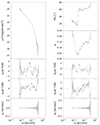 |
Fig. D.2. Same as in Fig. D.1, but for the galaxy WISEA J124839.70-411605.1. |
| In the text | |
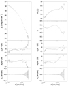 |
Fig. D.3. Same as in Fig. D.1, but for the galaxy WISEA J124831.02-411823.2. |
| In the text | |
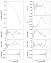 |
Fig. D.4. Same as in Fig. D.1, but for the galaxy WISEA J124902.02-411533.7. |
| In the text | |
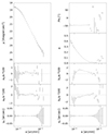 |
Fig. D.5. Same as in Fig. D.1, but for the galaxy WISEA J124846.61-411539.4. |
| In the text | |
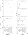 |
Fig. D.6. Same as in Fig. D.1, but for the galaxy ESO 322- G 093. |
| In the text | |
|
Fig. E.1. Comparison between the input and output magnitudes for the artificial stars’ experiment in the i′ band. The dots the means of the difference between the input and output magnitudes (MAGadd − MAGiso), whereas the errorbars are their RMS. |
| In the text | |
Current usage metrics show cumulative count of Article Views (full-text article views including HTML views, PDF and ePub downloads, according to the available data) and Abstracts Views on Vision4Press platform.
Data correspond to usage on the plateform after 2015. The current usage metrics is available 48-96 hours after online publication and is updated daily on week days.
Initial download of the metrics may take a while.