| Issue |
A&A
Volume 687, July 2024
|
|
|---|---|---|
| Article Number | A228 | |
| Number of page(s) | 22 | |
| Section | Stellar atmospheres | |
| DOI | https://doi.org/10.1051/0004-6361/202348808 | |
| Published online | 17 July 2024 | |
The IACOB project
X. Large-scale quantitative spectroscopic analysis of Galactic luminous blue stars★
1
Universidad de La Laguna, Dpto. Astrofísica,
38206
La Laguna,
Tenerife,
Spain
2
Instituto de Astrofísica de Canarias, Avenida Vía Láctea,
38205
La Laguna,
Tenerife,
Spain
e-mail: This email address is being protected from spambots. You need JavaScript enabled to view it.
3
Universität Innsbruck, Institut für Astro- und Teilchenphysik,
Technikerstr. 25/8,
A-6020
Innsbruck,
Austria
4
LMU München, Universitätssternwarte,
Scheinerstr. 1,
81679
München,
Germany
Received:
30
November
2023
Accepted:
20
February
2024
Abstract
Context. Blue supergiants (BSGs) are key objects for understanding the evolution of massive stars, which play a crucial role in the evolution of galaxies. However, discrepancies between theoretical predictions and empirical observations have opened up important questions yet to be answered. Studying statistically significant and unbiased samples of these objects can help to improve the situation.
Aims. We perform a homogeneous and comprehensive quantitative spectroscopic analysis of a large sample of Galactic luminous blue stars (a majority of which are BSGs) from the IACOB spectroscopic database, providing crucial parameters to refine and improve theoretical evolutionary models.
Methods. We derived the projected rotational velocity (υ sin i) and macroturbulent broadening (υmac) using IACOB-BROAD, which combines Fourier transform and line-profile fitting techniques. We compared high-quality optical spectra with state-of-the-art simulations of massive star atmospheres computed with the FASTWIND code. This comparison allowed us to derive effective temperatures (Teff), surface gravities (log 𝑔), microturbulences (ξ), surface abundances of silicon and helium, and to assess the relevance of stellar winds through a wind-strength parameter (log Q).
Results. We provide estimates and associated uncertainties of the above-mentioned quantities for the largest sample of Galactic luminous O9 to B5 stars spectroscopically analyzed to date, comprising 527 targets. We find a clear drop in the relative number of stars at Teff ≈ 21 kK, coinciding with a scarcity of fast rotating stars below that temperature. We speculate that this feature (roughly corresponding to B2 spectral type) might be roughly delineating the location of the empirical terminal-age main sequence in the mass range between 15 and 85 M⊙. By investigating the main characteristics of the υ sin i distribution of O stars and BSGs as a function of Teff, we propose that an efficient mechanism transporting angular momentum from the stellar core to the surface might be operating along the main sequence in the high-mass domain. We find correlations between ξ,υmac and the spectroscopic luminosity 𝓛 (defined as Teff4 / g). We also find that no more than 20% of the stars in our sample have atmospheres clearly enriched in helium, and suggest that the origin of this specific subsample might be in binary evolution. We do not find clear empirical evidence of an increase in the wind strength over the wind bi-stability region toward lower Teff.
Key words: techniques: spectroscopic / stars: abundances / stars: evolution / stars: fundamental parameters / stars: massive / supergiants
Full Table D.1 is available at the CDS via anonymous ftp to cdsarc.cds.unistra.fr (130.79.128.5) or via https://cdsarc.cds.unistra.fr/viz-bin/cat/J/A+A/687/A228
© The Authors 2024
 Open Access article, published by EDP Sciences, under the terms of the Creative Commons Attribution License (https://creativecommons.org/licenses/by/4.0), which permits unrestricted use, distribution, and reproduction in any medium, provided the original work is properly cited.
This article is published in open access under the Subscribe to Open model. This email address is being protected from spambots. You need JavaScript enabled to view it. to support open access publication.
1 Introduction
Massive stars (Mini ≳ 8 M⊙) play a pivotal role in galactic systems, exerting a profound impact on their chemo-dynamical evolution. On the one hand, massive stars make a substantial contribution to the chemical enrichment of galaxies, primarily through supernova explosions, but also through the release of enriched material via stellar winds (e.g., Maeder 1981; Woosley & Weaver 1995; Kaufer et al. 1997; Nomoto et al. 2013). On the other hand, their dynamic influence extends to the surrounding interstellar medium, driven by intense stellar winds and the copious emission of UV radiation. These factors can profoundly shape the interstellar environment (e.g., Krause et al. 2013; Watkins et al. 2019; Kim et al. 2019; Geen et al. 2021), either triggering or inhibiting new episodes of star formation.
These stars are intricately connected to some of the most energetic and dynamic phenomena in the Universe, such as core-collapse supernovae and gamma-ray bursts (Woosley & Bloom 2006; Smartt 2009). Additionally, their role has recently attracted attention in the realm of gravitational-wave astrophysics as they serve as progenitors of black hole and neutron star mergers (Abbott et al. 2016; Belczynski et al. 2016; Marchant et al. 2016).
Furthermore, massive stars are valuable tools for extragalac-tic research, serving as increasingly reliable distance indicators (Urbaneja et al. 2017; Taormina et al. 2020) and providing unique insights into the present-day abundances of their host galaxies (Bresolin et al. 2007, 2016; Kudritzki et al. 2012), even at distances spanning several megaparsecs (Kudritzki & Przybilla 2003; Urbaneja et al. 2003, 2005a; Kudritzki et al. 2008; Bresolin et al. 2022).
Blue supergiants (BSGs), a subset of massive stars, hold a crucial position in unraveling and understanding the intricate puzzle of the evolution of stars born with masses exceeding ≈15 M⊙. For a comprehensive overview of historical research and methodologies related to the study of BSGs, we refer to the introduction of a recent study by Weßmayer et al. (2022). Traditionally, BSGs were considered helium-burning stars that had completed their main sequence (MS) evolution as single stars (e.g., Hayashi & Cameron 1962). However, decades of observations have revealed persistent discrepancies with theoretical models, indicating that the evolutionary status of BSGs is much more intricate (see, e.g., Fitzpatrick & Garmany 1990; Castro et al. 2014; Wang et al. 2020). This complexity likely arises from a range of diverse evolutionary pathways that can ultimately populate the region on the Hertzsprung–Russell diagram where BSGs are located (see Vink et al. 2010; Maeder & Meynet 2012; Langer 2012). In this context, the compilation and analysis of spectroscopic data of BSGs with a considerable increase in quality and sample size compared to previous works (e.g., Dufton 1972; Lennon et al. 1992; Crowther et al. 2006; Lefever et al. 2007; Searle et al. 2008; Markova & Puls 2008; Castro et al. 2014; Haucke et al. 2018; Weßmayer et al. 2022) is becoming an urgent need to decipher a more complex scenario than the one initially established.
Focused on this and related aspects, the IACOB project1 started in 2008 with the overarching objective of providing high-quality empirical information on a statistically significant unbiased sample of Galactic massive stars. The aim was to establish new anchor points for testing and improving current theories of stellar atmospheres, winds, interiors, and the evolution of massive stars. Previous efforts of the IACOB team mostly concentrated on the study of line-broadening sources affecting the spectra of O- and B-type stars (Simón-Díaz & Herrero 2014; Simón-Díaz et al. 2014, 2017; Godart et al. 2017) and the empirical characterization of Galactic targets covering the O-star domain (Holgado et al. 2018,2020,2022; Britavskiy et al. 2023).
Within this framework, the aim of the study presented in this paper, which can be considered a continuation of de Burgos et al. (2023), is to perform a homogeneous estimation of the relevant spectroscopic parameters of the most extensive sample of Galactic luminous blue stars compiled to date, with a specific focus on BSGs with O9 to B5 spectral types. In forthcoming papers, we will complement the results presented here with additional information on the luminosities, masses, radii, and surface abundances of key elements such as silicon, carbon, nitrogen, and oxygen, to cover other important quantities defining the properties of the sample. Our ultimate objective is to establish a new highly improved empirical standard for the study of these stellar objects.
The paper is organized as follows. Section 2 presents the spectroscopic dataset and the sample of stars under study. Section 3 describes the methodology used to obtain estimates for the line-broadening and other relevant spectroscopic parameters. Section 4 summarizes the results of the analysis and compares them with previous studies. In Sect. 5 we discuss the results of the analysis for the different parameters in our analysis, and in Sect. 6 we present the summary and conclusions of the work.
2 Observational dataset and sample
This work makes use of the stellar sample described in de Burgos et al. (2023) and the associated spectroscopic data, which were collected from the IACOB spectroscopic database (for the latest review, see Simón-Díaz et al. 2020) and the ESO public archive. All considered spectra were obtained with the FIbre-fed Echelle Spectrograph (FIES) on the 2.56 m Nordic Optical Telescope (NOT), the High Efficiency and Resolution Mercator Echelle Spectrograph (HERMES) on the 1.2 m Mercator telescope, and the Fiber-fed Extended Range Optical Spectrograph (FEROS) on the 2.2 m MPG/ESO telescope that provide resolving powers between R = 25 000 and R = 85 000. The median signal-to-noise ratio (S/N) of the compiled dataset is ≈ 130 at 4500 Å. All spectra have a common wavelength coverage between 3800 and 7000 Å, reaching 9200 Å in some cases. Figure 1 shows some examples of the quality of the spectroscopic observations that were analyzed in this work.
Our original sample comprises 666 stars of types O9–B9 selected from de Burgos et al. (2023). In that work, we used the effect of gravity on the shape of Hβ line as a proxy for the spectroscopic luminosity, log(ℒ/ℒ⊙) (see Sect. 4.4). Specifically, we used the quantity FW3414 (Hβ), defined as the difference between the width of the Hβ measured at three-quarters and one-quarter of its line depth, to select all O- and B-type stars with initial masses above ≈20 M⊙. This quantity represents an improvement over the traditional full width at half maximum (FWHM) by breaking the degeneracy caused by the projected rotational velocity (υ sin i), while minimizing other effects such as surface temperature and spectral resolution (see further notes in de Burgos et al. 2023).
Concerning luminosity classes2, our initial sample comprises 339 supergiants (class I), 113 bright-giants (class II), 111 giants (class III), 55 subgiants (class IV), and 48 dwarfs (class V). We note that this sample excludes 12 B-type hypergiants, 27 classical Be-type stars (see Negueruela 2004, and references therein), as well as 56 double-line or higher-order spectroscopic binaries (SB2+), identified in de Burgos et al. (2023). This was done due to the impossibility of analyzing these objects with standard 1D atmospheric models.
3 Analysis methodology
In this section, we describe the methodology used to derive the line-broadening and spectroscopic parameters of the stars in the sample. The analyses were carried out using the best available spectrum for each star (as quoted in Table D.1), not only based on the S/N but also regarding any potential issue affecting the spectral windows where the main diagnostic lines are located.
3.1 Rotational and macroturbulent velocities
Following Simón-Díaz & Herrero (2014), we used IACOB-BROAD to perform the line-broadening analysis. We obtained estimates of υ sin i using the Fourier transform and the goodness-of-fit techniques. The latter also provided us with estimates of the macroturbulent velocity (υmac, hereafter also referred to as macroturbulence). We checked the agreement of both techniques for deriving υ sin i, and decided to keep the values from the goodness-of-fit as our final estimates. The few cases with larger differences (≈20 km s−1) were attributed to low S/N spectra. Following de Burgos et al. (2023), we used Si III λ4567.85 Å and Si II λ16371.37 Å for this analysis.
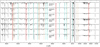 |
Fig. 1 Some illustrative examples of spectra used in this work, ordered by spectral type. Three different spectral windows depict the wavelength ranges in which the main diagnostic lines used to obtain estimates of the spectroscopic parameters are located. The vertical red, cyan, and brown bars indicate the corresponding H I, He I–II, and Si II–III–IV lines (see Sect. 3.2.3 for further details). |
3.2 Quantitative spectroscopy
3.2.1 Model atmosphere–line formation code and main assumptions
The NLTE model atmosphere and line synthesis code FASTWIND (Fast Analysis of STellar atmospheres with WINDs, v10.4.7, Santolaya-Rey et al. 1997; Puls et al. 2005, 2020; Rivero Gonzalez et al. 2011) was used to create a set of models for the analysis. A complete description of the current status of the code, as well as comparisons with alternative codes, have been presented by Carneiro et al. (2016). FASTWIND solves the radiative transfer problem in the comoving frame3 of the expanding atmospheres of early-type stars in a spherically symmetric geometry, under the constraints of energy conservation and statistical equilibrium, and accounting for line-blocking and line-blanketing effects. Homogeneous chemical composition and steady state are also assumed. The density stratification is derived from the hydrostatic balance in the lower atmosphere, and from the mass-loss rate and the wind-velocity field (a standard β-law) via the equation of continuity in the wind. A smooth transition between the wind regime and the pseudo-static photosphere is enforced.
Each FASTWIND simulation is defined by a set of parameters: the effective temperature (Teff), surface gravity (log 𝑔), and stellar radius (R), which are defined at τRoss = 2/3, the micro-turbulent velocity (ξ), the exponent of the wind-velocity law (β), the mass-loss rate (M), the wind terminal velocity (υ∞), and a set of elemental chemical abundances. Regarding any specific information concerning the detailed model atoms used in our calculations, we refer to Urbaneja et al. (2005b).
3.2.2 Grid of model atmospheres
As described in the previous section, each FASTWIND model requires a set of seven parameters (plus elemental abundances). However, the optical spectrum of typical B-type supergiants (such as those analyzed in this work) does not contain relevant information that would allow us to constrain all these parameters in parallel. For example, the main signature of the stellar wind is imprinted into the Hα profile, which for the most part is sensitive to the shape of the velocity field (i.e., β) and the wind-strength parameter (optical depth invariant) Q, a combination of mass-loss rate, wind terminal velocity and stellar radius4, and not to the individual values of these three physical parameters. Nothing can be said about possible inhomogeneities likely to be present in the outflow, since only Hα, a recombination line, is available. Based on these considerations, we decided to consider only homogeneous winds (i.e., without clumping) since at the very least they will provide an upper limit for the wind strength via Q.
In consequence, each model in our grid is defined by a set of seven parameters: Teff, log 𝑔, ξ, β, Q, helium and silicon abundances. The range covered by each parameter is indicated in Table 1). In addition, (a) following Urbaneja et al. (2011) we used a fixed ξ =10 km s−1 for the calculation of the atmospheric structure and occupation numbers, but allowed for different (depth-independent) microturbulences for the calculation of the line profiles (formal solutions); (b) we selected the lower limit of the effective temperature based on the fact that our models have not been thoroughly tested below Teff ≈ 14 kK; (c) the lower boundary for the helium abundance was selected to be the solar value (Magg et al. 2022), YHe = N(He)/N(H) = 0.10, as typically adopted in studies of Galactic massive stars; and (d) all other elements beyond helium and silicon are adopted to follow the solar metallicities as in Asplund et al. (2009).
To avoid the computation of an extremely large number of models that would be required in a classic regularly-spaced grid (reaching ≈1.5×10⁶ if we consider typical step-sizes in the sampling of the various considered parameters5), we opted for sampling the multi-D parameter space with a distribution of points following a Latin Hypercube Sampling algorithm (LHS; McKay et al. 1979; Wei-Liem 1996, see also Appendix A). The resulting analysis grid comprises 358 FASTWIND models (≈55 per dimension in the parameter space). Using supervised learning techniques, these models are employed to train a statistical emulator (Mackay 2003). This emulator is capable of reproducing FASTWIND simulations to a specific degree of fidelity in a fraction of the time required to run any actual simulation (Urbaneja, in prep.). Later on, during the inference phase (see 3.2.4), this emulator is utilized in combination with a Metropolis-Hasting algorithm (Metropolis et al. 1953) to sample from the underlying probability distribution.
Parameter space covered by the model atmosphere calculations used in the present work.
3.2.3 Diagnostic lines
Table 2 compiles the list of diagnostic lines chosen for this work. These were selected to be present in the 4000–7000 Å wavelength range, common to all the available spectra. Their location is shown in Fig. 1 with different colors depending on the atomic element.
These lines represent a minimum set required to obtain information on the fundamental atmospheric parameters characterizing the atmospheres of B-type supergiant stars. In particular, Teff is inferred from the ionization balances He I/II and Si II/III/IV (see for example McErlean et al. 1999; Urbaneja et al. 2005b). The hydrogen Balmer lines provide a strong constraint on log 𝑔, due to their sensitivity to broadening via the Stark effect. When the stellar wind becomes strong enough, the shape and strength of the Hα profile can provide constraints simultaneously on the wind acceleration β and Q.
The microturbulent velocity is estimated from the differential response of the three components of the strong Si III λλ4553– 68–75 Å triplet. We also note that some He I lines could show some sensitivity to this parameter (McErlean et al. 1999). However, the differential effect in the Si III lines is the dominant source of information. Finally, the surface abundances are determined from the strength of the corresponding spectral lines of each species.
Strictly speaking, however, all the spectral features can (and will) react to more than one of the fundamental stellar parameters. For example, the hydrogen Balmer lines are also sensitive to Teff and the helium abundance, albeit to a lower degree than to log 𝑔. Similarly, the helium lines do not only depend on Teff and helium abundance but also on log 𝑔 and ξ. Therefore, the analysis methodology involves a multi-dimensional optimization problem, in which the best solution is found in an iterative process, assuring at the same time a proper exploration of the full parameter space (see below).
In addition to the physical arguments, when selecting lines, we avoided choosing those that are affected by known issues, for example showing blends with atomic species not currently included in our detailed model atoms, as well as lines that are severely affected by the presence of telluric lines. For example, the H∈ line was excluded due to contamination with the strong interstellar calcium line.
Spectral features that show systematic differences between models and observations, suspected of suffering from modelling issues, were also excluded from the beginning. This is the case for the prominent He I λ6678 Å line, for which our models always predicted narrower lines than observed, which suggests that our current broadening data for this particular line are not fully adequate for B-type supergiant stars (see also Sect. 3.2.5 for other less important issues).
For each diagnostic line indicated in Table 2, the length of the corresponding spectral window used for the analysis was adjusted individually, taking into account the different intrinsic and rotational broadening. We also note that all the listed lines were always accounted for during the analysis process, even if a line was weak or not present. This is because such situations still provide important information (e.g., the absence of the He II λ4542 Å (see Fig. 2) indicates that the effective temperature of the star cannot exceed a certain value).
In addition, any contamination due to blends with lines from other species was masked out. We illustrate this in Fig. 2, where we show the same spectral window for four different stars with their associated masks. It can be seen that the selected regions (in green) are different in all the cases, being more restrictive for the bottom right panel, where multiple blends are present.
List of diagnostic lines used for the determination of the spectroscopic parameters.
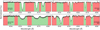 |
Fig. 2 Examples of different masks used to select the diagnostic lines. Each of the four panels shows the same wavelength range including the He II λ4542 Å line and the Si III λλ4553,4568,4575 Å triplet. The two panels on the left compare two stars of similar temperature but different υ sin i: HD 14 302 with υ sin i ≈ 65 km s−1 (top left), and HD 197 460 with υ sin i ≈ 200 km s−1 (bottom left). The two panels on the right compare two stars of similar υ sin i but very different Teff : HD 24 432 with Teff = 15 kK (top right) and HD 190991 with Teff =32kK (bottom right). The wavelength ranges selected for each analysis are shaded in green. The masked (not used) regions are shaded in red. |
3.2.4 Parameter inference
The problem of determining the set of parameters  defining the model Mλ that best reproduces an observation Oλ can be mathematical described as finding the underlying probability distribution:

There,  represents the prior knowledge that we have on the models, and
  is the likelihood of an observation Oλ given the model Mλ.
A well-proven method to sample from this unknown posterior distribution, to recover the best parameter set and their corresponding uncertainties, is the use of a Markov chain Monte Carlo (MCMC) algorithm (Metropolis et al. 1953; Chib 2001). Key to the inference of the parameters is the definition of what is considered “best” (i.e., what criteria are used to evaluate the likelihood of a model, given an observed spectrum), as well as the prior knowledge on the parameter space. For the likelihood function (i.e., the probability that a specific model Mλ defined by a set of parameters  fits a given observed spectrum O) we adopt Eq. (1) (see Mackay 2003)
 (1)
(1)
where for each diagnostic window defined to contain the lines in Table 2, the merit function χ is defined as the sum of the quadratic residuals, weighted by the uncertainties, and normalized to the effective number of wavelength points np contributing to the sum. Hence for each window, this corresponds to
 (2)
(2)
Since in the construction of the Markov chain we are using emulated FASTWIND spectra and not direct simulations (see Sect. 3.2.2), we convinced ourselves that the level of accuracy obtained by the statistical emulator is good enough as not to affect the outcome of the analysis (i.e., that the possible uncertainties σe introduced in the synthetic line profiles due to the statistical nature of the emulation are always significantly below the photon-noise level σp). Therefore  .
.
Concerning the priors, we assume that each value within its predefined range (see Table 1) has the same probability (i.e., uniform priors). Additionally, each spectral window contributes with the same weight to the merit function. No differential weighting scheme is applied since we have a similar number of lines for all the species.
Once the marginalized posterior probability distribution functions (PDFs) are recovered, the values of the parameters and their uncertainties are defined according to the following cases: (a) In the best case, when the location of the uncertainties lies within the range of possible grid-values, the solution is taken as the location of the maximum of each marginalized PDF, whilst the uncertainties are obtained as the values corresponding to the first and third quartiles of the associated cumulative distribution functions. (b, c) A lower or upper limit, when the upper or lower uncertainties lie in the upper or lower boundary limit, respectively. (d) An undefined solution, when the difference between the lower and upper uncertainties extends to more than 70% of the range of possible values.
An exception to case c applies to the helium surface abundance, which, as indicated in Sect. 3.2.2, has the lowest value set to YHe =0.10. Formally then, the helium abundance is not properly determined in the analysis when its actual value is close to this value. However, the solar helium abundance limit is a reasonable ansatz for the problem at hand, and hence we adopt these cases as solutions (a).
An overview of the output obtained through the spectro-scopic analysis is included in Appendix B for HD 198 478, complemented with a corner plot to illustrate the covariance between different atmospheric parameters. We also included examples of the output distributions for each of the cases mentioned above.
3.2.5 Quality assessment of the solution
Given the large number of stellar spectra for which we intend to extract fundamental parameters, we decided to evaluate the quality of each solution by defining several quality indicators, each connected to some extent to one of the physical parameters: Hα as the only indicator of the quality of the wind strength; Hδ, Hγ, and Hβ Balmer lines as indicators of the surface gravity; Si II-III-IV and He I-II lines as separate indicators of the effective temperature through their ionization balances, and the Si III triplet for the microturbulence, as explained in Sect. 3.2.3. The spectral window associated with each line is evaluated regarding the residuals between the observed spectra and the solution model as
 (3)
(3)
where the tolerance ∈, defined as ∈ = [S /N]−1, is a measurement of how much deviation is allowed between observed (Oλ) and synthetic profiles (Mλ), and np is the number of wavelength points in the spectral window that effectively contributed to the evaluation of the goodness-of-fit. As a result of some systematic broadening issues in some of the lines (see below), high S/N values might lead to large χ2 values that do not necessarily indicate a bad solution. To reduce the effect caused by these systematics, we set 100 as the upper limit of the S/N.
For each quality indicator, except the one associated with the wind, we averaged the χ2 values of the associated lines. In the case of Si II-III-IV and He I-II, we first averaged over those lines that correspond to the same ionization stage. Finally, we used all the solutions in which Teff and log g correspond to case a (see Sect. 3.2.4) to obtain a histogram for each quality indicator (see Fig. 3 and Sect. 4.1).
We also examined the individual χ2 distributions of the silicon and helium diagnostic lines, which allowed us to identify systematic differences between observations and models. In particular, we found what appears to be a small but systematic difference in the broadening affecting the He I λ4387.93 Å and He I λ4921.93 Å lines. This could be related to issues with the forbidden components and not the broadening per se, and are in any case smaller than the differences found in He I λ6678 Å, which we considered large enough to be initially excluded from the analysis. We also found difficulties in reproducing He I λ5875.62Å when the effect of the wind becomes relevant. We decided to exclude these three lines only from the following quality assessment.
To provide a single quality flag (q) that reflects the overall goodness of each solution, we used the above-mentioned histograms to consider four cases (from better to worse):
q1: When each of the five values of χ2 lies within 3-σ of the distribution after applying an iterative clipping of the outliers until convergence is achieved. This corresponds to a very good overall fit of all the diagnostic lines and the best reliability of the derived parameters.
q2: When the value of χ2 associated with Hα lies outside 3– σ of the corresponding distribution (see second panel of Fig. 3), a situation which is normally indicating a less-optimal fit to the specific profile-shape of this line (see the two examples in Fig. 4). As the purpose of this work is not to provide an accurate description of the wind properties, we consider this group to be the second best if all other four values lie inside 3-σ.
q3: When one of the values of χ2 associated with the gravity determination, the helium or silicon ionization balances, or the microturbulence lies outside 3-σ of the corresponding distribution (see panels 1, 3, 4, and 5 in Fig. 3, respectively), indicating potential issues with the estimation of log g, Teff, ξ, or surface abundances.
q4: The same as q3, but with two or more values of χ2 lying outside 3-σ. This corresponds to the worst case and is typically associated with problems in the spectrum (e.g., low S/N or normalization issues).
We note that q3 and q4 are independent of q2 and therefore one solution can simultaneously attributed to q2 and q3 or q4. Some examples of the different flags are presented in Fig. 4, where a comparison between observed and synthetic profiles can be found.
 |
Fig. 3 Histograms of the five quality indicators described in Sect. 3.2.5, each connected to a physical property, as indicated in the label of each panel. All histograms combine the information of all the stars with reliable estimates of Teff and log 𝑔. The gray bins correspond to values within 3-σ after applying an iterative clipping until convergence is achieved, while the red bins correspond to the clipped values. The median and 3-σ values are indicated in the figure with vertical and dash-dotted blue lines, respectively. The associated values are shown in the legend. For the panel associated with the wind strength, the x-axis extends to significantly higher values than for the others. |
4 Results
4.1 General outcome from the analysis
Given the boundaries in Teff and log g of our considered grid of models, we were able to obtain estimates for a total of 527 stars (i.e., they belong to case a as defined in Sect. 3.2.4). The corresponding quality distribution will be detailed later below, but we anticipate already here that the majority of stars (86%) belongs to q1.
The remaining 140 of the initial 666 O9–B9 type stars are not considered in the following sections and figures. They correspond to cases in which Teff or log 𝑔 are lower or upper limits (cases b and c, respectively), or to undefined solutions (case d). Concerning Teff, we found no stars with case b, indicating that all O9 stars fit within the limits of the grid, but we found 57 stars with case c, corresponding to B6–B9 stars with Teff values lower than the cold boundary of the considered grid of FASTWIND models (see Table 1). Regarding log 𝑔, 5 stars correspond to case b, and 34 to case c, the latter being mainly early-B giants and dwarfs. In 22 cases, we found a combination of the previous cases. The remaining 22 stars correspond to undefined solutions.
Table 3 provides a summary of the typical formal uncertainties associated with each investigated parameter. Although our analysis provides a lower and upper error for each parameter, both were very similar (on average, less than 10% different except for YHe), and we simply considered the average values for the table.
Figure 3 displays the histograms of χ2 for the five quality indicators described in Sect. 3.2.5. In each panel, the position of the 3-σ value used to assign the quality flags is included. Ideally, following Eq. (3), these values should gather around unity. It is evident that all the histograms except the one related to the wind strength have median values close to unity. This indicates that the chosen 3-σ clipping value is sufficiently stringent and that there are no significant systematic errors. In these cases, we also obtained similar 3-σ values. However, the histogram associated with the wind strength (Hα) displays larger median and 3-σ values, approximately three times larger. We will return to this problem in Sect. 5.5.
Following the criteria described in Sect. 3.2.5, we assign one of the four quality flags to each of the solutions. The percentages of solutions associated with each of them are: 83% for q1,9% for q2, 7% for q3, and 1% for q4. Remarkably, we can see that most of them are concentrated in q1, indicating an overall high quality of our results. The second largest group corresponds to q2. This, together with the fact that there are only six q4 cases, and those in q3 correspond to spectra with low S/N or specific issues6, tells us that the considered grid is suitable for the analysis of the stars that fit within the boundaries of Teff and log 𝑔.
The basic information about the stars in the sample is summarized in the first columns of Table D.1. They include an identifiable name (ID) in the SIMBAD astronomical database (Weis & Bomans 2020), the Galactic coordinates, and the spectral classification. The following columns summarize the main outcome of the analysis, including the estimates of the rotational and macroturbulent velocities (columns υ sin i and υmac), and the estimates of Teff, log 𝑔, ξ, YHe and log Q (columns are named with the abbreviations from Table 1). Except for Teff and log 𝑔, each of these columns is preceded by an additional column "l," indicating which of the four possible scenarios for the probability distribution applies (see Sect. 3.2.4). In particular, the upper and lower limits are indicated with < and >, the degenerate cases with “d,” and the rest are considered reliable with an equals sign (=). An extra column named “q” indicates the corresponding quality flag (q1–q4). The last two columns indicate the name of the fits-file in the format of the IACOB spectroscopic database corresponding to the best spectrum, and the associated S/N in the 4000–5000 Å region.
As indicated in Sect. 1, metal abundances will be discussed in a forthcoming paper; however, we briefly summarize here the main outcome of our spectroscopic analysis regarding silicon abundances. Globally speaking, the associated distribution has a mean and a standard deviation of 7.46 and 0.14 dex, respectively. This result is consistent with Hunter et al. (2009), who considered 56 Galactic B-stars (less than half of which were supergiants) located in specific clusters, obtaining ∈Si = 7.42 ± 0.07 dex. Also, we find a fairly good agreement with Nieva & Przybilla (2012) who obtained ∈si = 7.50 ± 0.05 dex using a sample of 20 Galactic B-type dwarfs in the Solar vicinity. Interestingly, the standard deviation of our distribution of estimated abundances is somewhat larger compared to Hunter et al. (2009), Nieva & Przybilla (2012), and also compared with the typical uncertainties resulting from our analysis (see Table 3); however, this could be related to the fact that, as shown in de Burgos et al. (2020), our sample includes stars from many different locations and is certainly not limited to stars within 500 pc from the Sun as in Nieva & Przybilla (2012), but up to 3–4 kpc instead. Further results and discussions on these issues will be presented in a follow-up study.
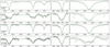 |
Fig. 4 Four illustrative cases of the quality labels assigned to the solutions (see text). Each row is divided into three spectral windows presenting three of the diagnostic regions: Si III λλ4553–68–75 triplet (left); He I λ4471 (middle); and Hα (right). The dashed green line is the synthetic spectrum of the model with the best-fitting parameters; the solid black line is the observed spectrum. |
Summary of the formal uncertainties obtained for each parameter.
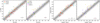 |
Fig. 5 Comparison of the results of the Teff and log 𝑔 with previous studies in the literature. The acronyms follow those used in Table 4. The error bars in the bottom right corners indicate the average uncertainty from our analysis (vertical axis) or from the literature (horizontal axis) except for those from Weßmayer et al. (2022) for which a separate error bar in pink is included. The two shaded areas indicate a difference in Teff and log 𝑔 of 1000 K and 0.1 dex, and 2000 K and 0.2 dex, respectively. The diagonal black line indicates the 1-to-1 agreement. |
Summary of the analyses used by other studies of Galactic luminous blue stars.
4.2 Comparison with previous results
Figure 5 compares our results for Teff and log 𝑔 with other relevant studies in the literature that also performed quantitative spectroscopic analysis on small- or medium-sized samples of Galactic luminous blue stars. They are separated into two groups to better illustrate the differences. Table 4 summarizes the main characteristics of the different analyses used by those works and the number of stars in common. The table also includes the different acronyms used to refer to each of those works. In most cases, they have made use of the atmospheric codes CMFGEN (Hillier & Miller 1998), or FASTWIND as also done here. Other cases include the use of TLUSTY (Hubeny 1988) or ATLAS 12 (Kurucz 2005) combined with DETAIL (Giddings 1981) and SURFACE (Butler & Giddings 1985). In McErlean et al. (1999), Crowther et al. (2006), and Searle et al. (2008) (first and third panels of Fig. 5), the typical formal uncertainties in Teff and log 𝑔 are ≈2000 K and ≈0.2 dex, respectively. In Lefever et al. (2007), Markova & Puls (2008), and Haucke et al. (2018) (second and fourth panels), the uncertainties are on average ≈800K and ≈0.1dex, respectively. Weßmayer et al. (2022) claims the smallest average uncertainties of ≈250 K and ≈0.05 dex. We note that, except for Weßmayer et al. (2022), the quoted uncertainties are systematically larger than those reached in our analysis (see Table 3); this is mostly a consequence of our analysis method and the way our uncertainties are derived.
The different strategies and methodologies used in those works made it very difficult to assess the overall agreement with our results, as well as to carry out individual comparisons. Despite this, we provide some individual notes and try to explain the reasons for some of the more notorious differences.
First, we find a good overall agreement with the results of McErlean et al. (1999), one of the first studies attempting to derive spectroscopic parameters for a large sample of BSGs. Most of the results lie within ±1000K and ±0.1 dex as shown in the corresponding panels of Fig. 5. This is interesting as it is a study with large differences in the methodology, as they used plane-parallel geometry and unblanketed models.
The comparison with Crowther et al. (2006) also shows a very similar situation. However, one main difference from this work is their use of a fixed YHe =0.2 which, as shown in Sect. 5.4), is not a representative value for the majority of the analyzed luminous blue stars. Comparing the fit quality for those stars with differences in Teff or log 𝑔 larger than 1000 K or 0.1 dex, respectively, we find a typically better quality from our results.
In the case of Searle et al. (2008), we observe a larger scatter of the differences, both in Teff and log 𝑔. The latter was also found by the authors themselves when comparing with Crowther et al. (2006), being of the order of 0.1–0.2 dex. Despite that they attributed this difference to wind contamination of the Balmer lines, one also finds differences in some diagnostic metallic lines and significant discrepancies between their fitted and observed spectra.
The differences with McErlean et al. (1999), Crowther et al. (2006), and especially Searle et al. (2008) might also be attributed to the much lower resolutions used in those works compared to our data. Moreover, none of these works accounted for macroturbulent broadening, which can represent an important contribution to the shapes of the lines.
Our comparison with Lefever et al. (2007) shows the largest discrepancies with our results, with lower Teff and log 𝑔 values for many of the stars in common. One reason for this difference could betheir(much) lowernumberofdiagnosticlines compared to other studies. In particular, they only used Hγ as the primary gravity indicator and He I λ4471.47 Å in the second place. For Teff they used either the Si II4130 Å doublet or the Si III 4560 Å triplet. They also adopted a fixed solar silicon abundance, which can also affect the determination of the effective temperature.
The study by Markova & Puls (2008) represents the closest comparison to our methodology. However, the number of stars in common is very limited. Nevertheless, we observe a good agreement for almost all stars in common.
The results from Haucke et al. (2018) show a good agreement for half of the stars in common, with the other half having lower Teff and log 𝑔 values than in our case. For these stars, we found (as also by the authors) that their Teff and log 𝑔 values are systematically lower compared to other studies such as Crowther et al. (2006) or Searle et al. (2008).
Last, our results compared to Weßmayer et al. (2022) show a good agreement despite the different methodologies and the fact that they account for the effects of turbulent pressure on the models. We could only identify a slight trend toward lower Teff in their case. The authors suggested (via private communication) that the differences are likely due to differences in the silicon model, especially affecting some Si II lines (see Weßmayer et al. 2022, for more details).
In summary, we do not see any particular trend in our results that may indicate a problem with our models or with the analysis technique. We also do not find particular differences when comparing the results obtained with FASTWIND or CMFGEN. Regarding the largest differences, they were attributed in the first place to specific reasons related to the fit quality (e.g., Searle etal. 2008), orthe absence ofdiagnostic lines (e.g., Lefever et al. 2007).
4.3 Teff –spectral type calibration
Several studies have obtained calibrations of spectral type against Teff for Galactic BSGs in the past (see Lefever et al. 2007; Markova & Puls 2008; Searle et al. 2008; Haucke et al. 2018). These calibrations are, however, based on samples of relatively small size, with no more than a few tens of targets in the best cases. Here, we benefit from our much larger sample to provide a revised calibration. Figure 6 shows Teff as a function of spectral type for those analyzed stars with luminosity classes Ia, Iab, and Ib. To avoid spurious results associated with the use of erroneous spectral classifications (as those provided by SIMBAD in many cases, see de Burgos etal. 2023, and Sect. 4.4), we highlight with blue dot symbols those stars with reliable spectral classifications as provided by Sota et al. (2011, 2014), de Burgos et al. (2020, 2023), and Negueruela et al. (2024).
Using only those stars in the former group, we performed both a linear and a third-order polynomial fit (the latter option first proposed by Lefever et al. 2007), accounting for individual errors in Teff. The resulting calibrations are:

where x is the spectral type adopting O9=−1, B0 = 0, and so on. Additionally, the 1-σ uncertainties for each spectral type are: O9 ± 1300 K, B0 ± 1500 K, B1 ± 700 K, B2 ± 700 K, B3 ± 600 K, where for the B4- and B5-type stars, they are not provided due to the reduced number of objects.
As illustrated in Fig. 6, both calibrations (indicated with black and gray dashed lines, respectively) are almost identical from O9 down to B3-type stars, but significantly differ for later types. We also see a much larger scatter in Teff for those stars whose classifications are directly extracted from SIMBAD (gray dot symbols).
Compared to previous calibrations by Lefever et al. (2007), Markova & Puls (2008), and Haucke et al. (2018), their regression curves seem to agree with our results only for B0-type objects, differing by 1–3 kK for O9 and B1–B5 spectral types. The explanation for this difference is the considerably smaller number of targets considered by these authors, together with the change of slope beyond the B5 spectral types, which notably modify the polynomial fits. Taking into account the improved statistics, our calibration is clearly more robust than the other three.
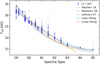 |
Fig. 6 Teff against spectral type for stars with luminosity class I. The blue dots correspond to stars with revised classifications (see Sect. 4.3), whereas the gray dots correspond to stars whose classification corresponds to the default provided by SIMBAD. The dashed orange and cyan lines correspond to a first- and third-order polynomial fit to the stars in blue. Some previous calibrations from the literature are also included for comparison. |
4.4 Spectroscopic HR diagram
The location of the sample stars in the spectroscopic Hertzsprung–Russell diagram (hereafter sHR diagram Langer & Kudritzki 2014) is shown in Fig. 7, where we also indicate the boundaries of our model grid. Along with the stars in our study, the figure also includes 191 O-type stars from Holgado et al. (2018, 2020, 2022, hereafterHol18-22).
The colors in Fig. 7 indicate the luminosity class of the stars as listed in Table D.1. In particular, for most of the stars in the sample, we adopted the recommended classifications quoted in SIMBAD. However, as shown in de Burgos et al. (2023), for B-type stars, a nonnegligible number of luminosity classes in SIMBAD are incorrect or not even provided (see also Fig. 6). While we plan to review the spectral classifications of all B-type stars in our sample following the guidelines of Negueruela et al. (2024), for this work we keep using the SIMBAD classifications except for those ≈ 120 stars for which we have published revised spectral types and luminosity classes (see de Burgos et al. 2020, 2023; Negueruela et al. 2024). These revised classifications represent an improvement for supergiant stars (see for comparison Fig. 5 in de Burgos et al. 2023).
As illustrated in Fig. 7 (see also Sect. 2), the majority of stars in our sample (≈70%) comprise stars with luminosity classes I and II, especially toward cooler temperatures (below Teff < 29 kK, see also Fig. 8). However, there is also a nonneg-ligible number of objects with luminosity class III, IV and V. Despite most of them being located close to the hot boundary of the investigated domain, there is still a fraction of objects from this latter group whose location in the sHR diagram overlaps with the region predominantly populated by stars with classes I and II. Following the criteria formulated in Negueruela et al. (2024), we revised the spectral classification for those class-V stars that overlap with the location of stars with luminosity class I, II, and III. Appendix C shows that almost all of them actually correspond to stars with class-III.
This result warns us again about the use of unchecked spectral classifications from SIMBAD. It also highlights the urgent need for a systematic revision of an important percentage of the known B-type stars, following a similar homogeneous approach as the work performed by Maíz Apellániz et al. (2011, 2016); Sota et al. (2011, 2014) in the case of O-type stars.
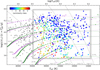 |
Fig. 7 sHR diagram showing our results from the analysis for 527 stars with O9–B5 spectral type color-coded by their luminosity class, and 191 O-type stars from Hol18-22 in gray. The boundaries of our model grid are indicated with a rectangle. The shaded area indicates the approximate region where our results correspond to the upper or lower limits (see Sect. 3.2.4). The approximate separation between the O- and B-type stars is indicated with a dotted diagonal black line. For reference, the figure includes nonrotating evolutionary tracks with solar metallicity from the Geneva and Bonn models (Ekström et al. 2012; Georgy et al. 2013; Brott et al. 2011, respectively). Intervals of the same age difference are marked with purple crosses for Geneva and green triangles for Bonn, which are connected with dashed and dash-dotted lines of the same color. The dash-dotted gray lines indicate different constant log g values. |
5 Discussion
5.1 An empirical hint for the terminal-age main sequence in the high-mass domain
The empirical identification of the location of the terminal-age main sequence (TAMS) provides important constraints for several physical phenomena occurring in the interior of stars along the main sequence, including core overshooting processes, and the impact of rotational mixing and magnetic fields, among others (see, e.g., Meynet & Maeder 2000; Vink et al. 2000; Maeder & Meynet 2005; Schootemeijer et al. 2019; Martinet et al. 2021; Scott et al. 2021). Above ≈3 M⊙, once hydrogen is exhausted in the convective core and the TAMS is reached, stars suffer from a rapid reconfiguration of their internal structure while evolving approximately at constant luminosity. In brief, they increase considerably their size (and hence the effective temperature decreases), while the inert core is contracting. As a consequence of the short time-scale of this process, the relative number of stars in a volume-limited sample detected on the cool side of the TAMS is expected to be considerably lower than those populating the main sequence.
Figure 8 depicts a histogram of the effective temperatures of the stars shown in Fig. 7. The relative number of stars in each bin steadily increases from the hot end down to ≈21 kK, where a clearly noticeable drop is detected. As indicated above, this drop might roughly delineate the location of the empirical TAMS in the mass range between 15 and 85 M⊙. Interestingly, this severe drop in the number of stars is located 5–7 kK below the theoretical TAMS predicted by the single-star evolutionary models of Ekström et al. (2012). Alternatively, if compared to the single-star models of Brott et al. (2011), the location of the drop overlaps well with the theoretical TAMS for masses below 40 M⊙, but for masses above, the TAMS is shifted to temperatures ≈10kK cooler. The large difference between both sets of models is mainly related to the different treatment of angular momentum transport (Ekström et al. 2012, advective; Brott et al. 2011, diffusive), and the different size of the core-overshoot parameter (lower in Ekström et al. 2012), where the latter has a large impact on the main-sequence lifetimes.
While the presence of BSGs beyond the theoretically predicted main sequence in single-star evolutionary models has been known for a while (see, for example, Fitzpatrick & Garmany 1990; Castro et al. 2014, using photometric and spec-troscopic observations, respectively), our work implies a higher statistical significance, given the large sample of stars homogeneously analyzed here. Should this location of the TAMS be confirmed, not all BSGs would be He-core burning post-MS stars, with a possible significant fraction of them (mostly those with spectral types earlier than B3) being H-core burning objects (see also previous hints by Vink et al. 2010; Brott et al. 2011; Castro et al. 2014; McEvoy et al. 2015).
However, the possibility of other evolutionary channels populating this part of the sHR diagram, mainly invoking post-mass transfer binaries and mergers (see Marchant & Bodensteiner 2023, and references therein), but also post-red supergiant stages through blue loops (e.g., Stothers & Chin 1975; Martinet et al. 2021; Zhao et al. 2023), complicates a definitive identification of BSGs as main sequence or post-main sequence objects just accounting from the simple picture described above. In addition, the potential impact of observational biases, as well as sampling effects related to the initial mass function and the age range of the compiled sample should be taken into account in any attempt to explain the observed distribution of stars presented in Fig. 7.
For example, despite one would expect a more or less constant distribution of stars as a function of effective temperature along the main sequence evolution, the relative number of stars in the Teff range ≈30–20 kK is noticeably larger than in the ≈40– 30 kK range (see Fig. 8). This could be partially explained by the effect of a Malmquist bias affecting our magnitude-limited sample (see de Burgos et al. 2023, for a detailed discussion). Since mid B-type supergiants are expected to be intrinsically brighter in the optical than other supergiants with similar luminosities but earlier spectral types, the distances reached for the former group are much larger than for the latter; hence, an overabundance of mid-to-late BSGs is expected in our sample. This strengthens our suggestion that the TAMS might be located at ≈21 kK if we assume the drop in density of stars as a function of Teff as empirical evidence of the position of the TAMS.
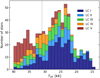 |
Fig. 8 Histogram of effective temperatures for all the stars in Fig. 7, color-coded by luminosity class. The approximate separation between O- and B-type stars is indicated with a dashed vertical black line. |
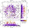 |
Fig. 9 sHR diagram of the 527 stars in the sample and 191 O-type stars from Hol18-22, all color-coded by v sin i. The bottom and right subpanels show υ sin i against Teff and log ℒ, respectively. The boundary limits of our grid of models are marked with dashed black lines. The evolutionary tracks are the same as in Fig. 7 for Geneva models. |
5.2 Rotational properties
Figure 9 shows an sHR diagram with the same stars as in Fig. 7, but color-coded by their projected rotational velocities. The central panel is complemented with another two (right and bottom subpanels) in which the measured υ sin i values are directly confronted against log ℒ and Teff, respectively.
As observed for Galactic O-type stars (see Holgado et al. 2022, and references therein), two main components can also be clearly distinguished in the υ sin i distribution when moving to the BSG domain (see also Fig. 10): one main component (comprising about 70% of the sample) with projected rotational velocities ranging from ≈10 km s−1 to ≈100 km s−1, and a tail of fast rotating stars reaching values of ≈400 km s−1. While the main component is present in the full range of covered effective temperatures, the tail of fast rotators disappears below ≈20kK (see bottom panel of Fig. 9).
The existence of a bimodal υ sin i distribution in the O star domain has been known for several decades (see, e.g., Conti & Ebbets 1977). This is also the case for the clear drop found in the Teff–υ sin i diagram at Teff ≈ 21 kK (see bottom panel of Fig. 9), which has previously been identified by several authors (see, e.g., Howarth et al. 1997; Vink et al. 2010; Fraser et al. 2010; Brott et al. 2011), including our previous work (de Burgos et al. 2023), where we found its location around the B2-type stars with luminosity class I and II.
A theoretical explanation for the occurrence of a bimodal distribution (proposed by de Mink et al. 2013) invokes the effect of mass transfer in binary systems, implying the spin-up of the gainer. In this scenario, which has found empirical support by Holgado et al. (2022) and Britavskiy et al. (2023), the tail of fast rotators is mostly populated by post-interaction binary products, and the observed υ sin i distribution is not necessarily representative of the initial spin-rate at birth of the investigated samples. This hypothesis leaves room for the possibility that the low-υ sin i component of the distribution mostly comprises stars which have not interacted with any companion, while also including some fast rotating stars seen with a low inclination angle, as well as potential mergers spun-down by magnetic fields (see, e.g., Schneider et al. 2016; Keszthelyi et al. 2019).
Thanks to the large sample of stars for which we have obtained υ sin i, Teff, log ℒ, and log Q estimates, and as a follow-up of the work started in Holgado et al. (2022), we can evaluate with good statistical significance and robustness how the observed υ sin i distribution is modified as stars evolve. To this end, we use Teff as a proxy of evolution, but also take into account that in the binary channel the direct relation between the Teff and age breaks down.
Figure 10 depicts the histograms of υ sin i for four subsamples of stars covering, from top to bottom, decreasing ranges of Teff. In particular, we consider three subsamples covering the region between our hotter Teff boundary and the speculated location of the TAMS (see Sect. 5.1), plus a fourth one comprising the supposedly post-MS region. In all cases, we mark the location of the mean υ sin i associated with the low-υ sin i component of the distribution and indicate the percentage of stars that have a υ sin i below 100 km s−1.
Regarding the low-υ sin i component, both Fig. 10 and the bottom subpanel of Fig. 9 show a slow decrease in its characteristic υ sin i (from 60 to 54 km s−1 in the Teff range between 40 and 21 kK, and from this later value down to 37 km s−1 when considering the cooler stars in the sample). This result is consistent with recent findings by Holgado et al. (2022) for the case of O-type stars, but also extending them further to lower effective temperatures. Despite the widely predicted loss of angular momentum due to stellar winds, the detected surface braking in the low-υ sin i component is almost negligible throughout the considered range of effective temperatures. As suggested by Holgado et al. (2022), this might be pointing toward the existence of an efficient mechanism transporting angular momentum from the stellar core to the surface along the main sequence. This statement might also be supported by the almost constant percentage of stars with υ sin i > 100 km s−1, as well as the maximum υ sin i values detected in the tail of fast rotators in stars ranging from the zero-age main sequence (ZAMS) to the suggested location of the TAMS (see Holgado et al. 2022, and Sect. 5.1).
Regarding the drop in υ sin i at Teff ≈ 21 kK, as pointed out by Vink et al. (2010), it could be either an indicator of the end of the main sequence or the result of an enhanced angular momentum loss at the theoretically predicted bi-stability jump (Pauldrach & Puls 1990; Vink et al. 1999, 2000)7 When considering this latter possibility, we must remember that the exact location and characteristics of the bi-stability jump remain a debated question (see Petrov et al. 2016; Krtička et al. 2024). There is not even consensus on the predicted occurrence of a significant increase in the mass loss rate when the star is crossing from the hotter to the cooler side of the bi-stability jump (Björklund et al. 2021, 2023). Furthermore, as described in Sect. 5.5, the behavior of our measured wind strength does not support a strong change of the mass-loss rate properties around the effective temperature where the drop in υ sin i is detected. Thus, we are still left with the question of what causes the observed drop in the υ sin i distribution as a function of Teff.
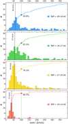 |
Fig. 10 Distribution of υ sin i separating the stars in the sample in four groups of different Teff ranges, as shown in the legends. The panels show the different histograms, indicating with a dash-dotted line the mean υ sin i values as derived from an iterative 2-σ clipping. In each panel the corresponding cumulative distribution and the percentage of stars with υ sin i < 100 km s−1 is also included. |
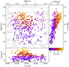 |
Fig. 11 sHR diagram of the stars in the sample color-coded by the ξ. The bottom and right subpanels show ξ against Teff and log ℒ, respectively. Results of ξ considered as upper or lower limits, or degenerated are excluded. The evolutionary tracks are the same as in Fig. 7 for Geneva models. |
5.3 Microturbulence and macroturbulence
Current analyses of the atmospheres of O- and B-type stars require the consideration of two broadening parameters, termed microturbulence (see, e.g., McErlean et al. 1998; Smith & Howarth 1998; Vink et al. 2000) and macroturbulence (e.g., Ryans et al. 2002; Simón-Díaz & Herrero 2014; Simón-Díaz et al. 2017), for which their exact physical origin is yet unknown. Figure 11 presents our derived microturbulences. Previous studies based on smaller numbers of stars in the B-stars domain have shown that supergiants have larger microturbulence values than giants and dwarfs (Gies & Lambert 1992; Hunter et al. 2007, 2008; Lefever et al. 2007; Markova & Puls 2008; Weßmayer et al. 2022). Benefiting from a much larger sample of stars, we investigated whether a connection between the spectroscopic luminosity and the microturbulence is statistically sound. A Spearman’s rank-order correlation of our results delivers a coefficient of ρ = 0.82 with a significance level of 95%, indicating the hypothesis of statistical independence between both quantities can be rejected.
Concerning the variation of ξ with respect to Teff for luminous blue stars (see, for example Markova & Puls 2008), we obtained a median value of 20 km s−1 for O9-B0.5, 17 km s−1 in the B0.5–B2 range, 15 km s−1 at B2–B4 type, and 12 km s−1 for B5 and later. We also notice an increased relative and absolute scatter toward the hotter Teff end, being particularly broad at Teff ≈ 26 kK, whereas a smaller scatter is present at the cool end.
Our derived macroturbulent velocities (υmac), combined with those from Hol18-22 for O-type stars, essentially reproduce the previous findings by Simón-Díaz et al. (2017) in terms of the dependencies with respect Teff and log ℒ, and hence are not repeated here. However, we go beyond that study in terms of investigating a potential correlation between ξ and υmac. Interestingly, Fig. 12 shows that a positive correlation does exist. To quantify this correlation we calculated Spearman’s correlation coefficient, which resulted in ρ = 0.71 at a significance level of 95%. This result deserves a follow-up, more in-depth study since it might indicate a connection between the physical drivers of the two broadening mechanisms.
Several plausible scenarios have been proposed to explain the occurrence of these two spectral line-broadening features. Among them, Cantiello et al. (2009) suggests that microturbulence originates in subsurface convective zones, whereas Grassitelli et al. (2015) and Cantiello et al. (2021) propose the same origin for macroturbulence. As an alternative, Aerts et al. (2009) suggested the collective pulsational velocity broadening due to gravity modes as a physical explanation for the macroturbulent broadening in hot massive stars. More recently, Aerts & Rogers (2015) extended further the proposed connection between macroturbulence and stellar variability phenomena by linking both through the effect of convectively driven waves originating in the stellar core (see also Edelmann et al. 2019; Lecoanet & Edelmann 2023; Anders et al. 2023). This latter scenario has been further explored by Bowman et al. (2019a,b, 2020), who also showed evidence of a correlation between the amplitude of observed stochastic low-frequency photometric variability, and the amount of measured macroturbulent broadening.
Overall, despite the various alternatives proposed, no firm conclusions have been reached yet (see, e.g., Simón-Díaz et al. 2017; Godart et al. 2017; Bowman et al. 2020; Cantiello et al. 2021). In these regards, the empirical correlations presented here and in Simón-Díaz et al. (2017), together with results from parallel works investigating the connection between macroturbulent broadening and photometric and line-profile variability (e.g., Simón-Díaz et al. 2010, 2017; Bowman et al. 2020) open new avenues to find more conclusive answers about the physical origin and potential connection between these two ubiquitous features.
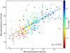 |
Fig. 12 Macroturbulence against microturbulence for the sample of stars, color-coded by their log(ℒ/ℒ⊙). The sample is limited to those stars with υ sin i < 100 km s−1. A linear fit is included and is indicated by a dashed diagonal black line. |
5.4 Surface helium abundance
Together with nitrogen and carbon, a consistent determination of the surface abundances of helium in O- and B-type stars can help to constrain the impact of internal mixing processes along the main sequence evolution (see, e.g., Martins et al. 2005; Rivero González et al. 2012; Carneiro et al. 2016; Grin et al. 2017). Furthermore, it can be used to identify the occurrence of mass transfer and merger events in massive binaries (see, e.g., Langer 2012; Langer et al. 2020; de Mink et al. 2013; Glebbeek et al. 2013; Schneider et al. 2016; Sen et al. 2022; Menon et al. 2023) and, ultimately, better identify the evolutionary status of the investigated targets (e.g., whether they are in a H- or He-core burning stage; see, Georgy et al. 2021, and references therein).
Figure 13 shows the sHR diagram for the estimated surface abundances of helium in our BSG and O-star sample. As in previous similar figures, we also present two subpanels to investigate potential dependencies between this quantity and log ℒ and Teff, respectively.
Globally speaking, our results cover the range YHe =0.10– 0.23, with few exceptions. For the discussion below, and based on the median of our results plus the average of all the error estimates for our sample stars, we define YHe = 0.13 as the threshold for a star to be considered He-enriched. We find that 20% of the stars in our sample have a surface helium abundance above this limit, of which only 7% display YHe > 0.16.
The right and bottom subpanels of Fig. 13 do not show any clear correlation between the amount of He surface enrichment and log ℒ or Teff. To further investigate the potential correlation between these three quantities, also taking into account the υ sin i of the stars, Table 5 summarizes some information of interest regarding the percentages of stars with YHe >0.13. This information is associated with subsamples of stars located within the 12 panels highlighted in red in Fig. 13. Specifically, we have selected three ranges in Teff that presumably cover the main sequence (see Sect. 5.1), plus a fourth one corresponding to stars with Teff < 20 kK (i.e., to the cooler side of the suggested empirical TAMS).
Notes. The first column refers to the panels displayed in Fig. 13. (a) Low- and high-υ sin i refer to stars with υ sin i below or above 100 km s−1, respectively. The indicated percentages have been computed with respect to the total number of stars in each υ sin i subgroup within the corresponding panel.(b) Abundances from Holgado (2019) are used for the 191 O-stars shown in Fig. 13.
Regarding stars with Teff > 20 kK, the most remarkable result is the particularly large percentage of He-enriched stars in panel a (reaching ≈60%); all other panels with Teff >20kK show only ≈10 to 20% of He-enriched objects, again without any correlation between this quantity and Teff or log ℒ. The statistics associated with the rightmost panels in Fig. 13 (d, h, and l) show a different behavior, with a much lower percentage of He-enriched stars (except for panel d).
Another interesting result is that in those panels where there is a clearly bimodal υ sin i distribution (namely those with Teff >20kK, see bottom subpanel of Fig. 13), the percentage of He-enriched stars in the tail of fast rotators is systematically higher (except for panel c) than for the main low-υ sin i component. A two-sample Kolmogorov-Smirnov test indicates that, with a 95% confidence, both groups (now also considering the non-He-enriched stars) do not arise from the same probability distribution for the surface helium abundance. This might be explained by attributing a different origin to the He-enriched stars in both low-υ sin i and fast-rotating stellar populations.
While we expect these results to serve as guidelines for future, in-depth comparisons of single and binary evolution model predictions, we provide here some first hints which can be extracted from the information in Table 5. First, we evaluate the possibility that He-enriched stars originate from single-star evolution. For this, we compare with evolutionary model predictions from Brott et al. (2011), Ekström et al. (2012), and Keszthelyi et al. (2022). Among them, only the models by Ekström et al. (2012) with an initial rotational velocity of 40% of critical rotation can explain some (but certainly not all, see below) of the percentages of stars with YHe > 0.13 quoted in Table 5. The alternative computations by Brott et al. (2011), and Keszthelyi et al. (2022) do not produce any remarkable He-enrichment along those main sequence tracks crossing any of the various red panels highlighted in Fig. 13.
Exploring further the evolutionary models computations by Ekström et al. (2012), we have found that they can, at maximum, explain 40-50% of the detected stars with He-enriched surfaces. Basically, these are targets with low and intermediate projected rotational velocities (υ sin i < 100–150km s−1) in panels a, b, e, and f. Whereas the observed percentage of stars with He-enriched surfaces is systematically larger within the tail of fast rotators (see above and Table 5), Ekström et al. (2012), on the other hand, predict that those stars with a clearly detected enrichment of helium should have also suffered from a significant braking of the stellar surface.
All this, together with the increasing empirical evidence indicating that main sequence massive stars might not be suffering from such a significant surface braking (see Sect. 5.2) leaves us with the necessity for an alternative scenario to explain an important fraction (if not all) of the detected He-enriched stars in our sample, particularly those with υ sin i > 150km s−1. In this context, given the high percentage of massive stars born in binary and multiple systems, and the high probability of an interaction during their evolution (see Marchant & Bodensteiner 2023, and references therein), stars that exhibit helium surface enrichment might be the result of binary interaction. For fast-rotating objects, they could be the gainers of post-interaction systems in which the mass transfer event occurs when the initially more massive star has evolved beyond the main sequence (i.e., case B mass transfer Langer et al. 2020; Wang et al. 2020; Klencki et al. 2020; Sen et al. 2022). Moreover, some of the He-enriched low-υ sin i stars could be the products of merger events, including cases in which the merging occurs when one or both components are close to or beyond the TAMS (see Podsiadlowski et al. 1992; Langer 2012; Schneider et al. 2016). Therefore, a more thorough investigation of the various possibilities opened by the binary channel, incorporating information about C, N, and O surface abundances and new predictions from single and binary evolutionary models, is hence certainly needed.
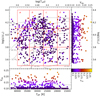 |
Fig. 13 sHR diagram of the stars in the sample plus 191 O-type stars from Hol18-22, color-coded by helium abundance. We adopted YHe ≈ 0.10 as the lowest possible value. The bottom and right subpanels show YHe against Teff and log ℒ, respectively. The various subgroups of stars listed in Table 5 are indicated with red solid lines. Results considered as lower limits or degenerate are excluded. The bottom subpanel includes a horizontal dotted line at YHe =0.13. The evolutionary tracks are the same as in Fig. 7 for Geneva models. |
Summary properties of He-enriched stars, separated in groups of different Teff and log(ℒ/ℒ⊙), as indicated in the second and third columns.
5.5 Wind properties
At present, several NLTE atmospheric codes are able to treat spherically extended atmospheres with winds (assuming radiative equilibrium). In this work we used FASTWIND (see Sect. 3.2.1), but other available codes are CMFGEN (Hillier & Miller 1998), PoWR (Gräfener et al. 2002; Hamann & Gräfener 2004), WM-BASIC (Pauldrach et al. 2001), or PHOENIX (Hauschildt 1992). A major challenge in reproducing the observed spectral lines affected by stellar winds is accounting for the inhomogeneities (clumping) of these winds (see Puls et al. 2008, and references therein). Such inhomogeneities can only be described by adopting a large number of free parameters (particularly, when modeling optically thick clumping, see, Sundqvist & Puls 2018), which significantly increase the complexity. However, recent studies have gradually tried to improve this scenario (see, e.g., Hawcroft et al. 2021; Brands et al. 2022; Bernini-Peron et al. 2023), since empirical constraints are key to derive important wind properties such as mass-loss rates.
In this work, we limit the discussion of such wind properties to our results for the wind-strength parameter8 and its relation to the morphology of the Hα line. In addition, more detailed investigations on the actual mass-loss rates and clumping properties will be presented in a forthcoming study.
Figure 14 displays the stars from Fig. 7, now colored by log Q. The results from Hol18-22 have been included for reference (in gray). The bottom subpanel shows two main and important features. First, our results do not show evidence for increasing mass-loss rates over the bi-stability region toward lower Teff. Instead, we observe a slow decay of the maximum log Q values, with log Q ≈ −13 in the 20–25 kK range. Second, we find a clear separation of two groups of stars below ≈22kK, one with log Q ≳ −13.6, and another one at (or below) log Q ≈ −14.0. We will return to this bimodal distribution later, when discussing the observed Hα morphology. Moreover, a diagonal gap dividing O- and B-type stars seems to be present.
The right-hand subpanel displays increasing log Q values with increasing log ℒ. This feature is expected since stars closer to the Eddington limit should and indeed do possess stronger stellar winds driven by intense radiation (see, e.g., Abbott 1980; Pauldrach et al. 1986). We also note that the wind strengths of stars with log(ℒ/ℒ⊙) ≲ 3.9 dex are considerably weaker (log Q ≲ −13.25) than those for values above.
Due to our neglect of wind inhomogeneities, discrepancies between the synthetic spectra from our best-fitting models and observations are to be expected, at least if the clumping properties would vary as a function of location (which seems to be the case, e.g., Najarro et al. 2011). In fact, these neglected inhomogeneities are the most likely contributors to the larger; χ2 values associated with the He line (see Fig. 3). Interestingly, the majority of cases where He could not be reproduced by our modeling correspond to profiles either displaying emission in both line wings or a P Cygni shape with very strong emission in the red wing. In some of these cases, the models were also unable to reproduce the shape of IIβ if it was not in pure absorption. Despite this, these results significantly increase the number of luminous blue stars for which wind-densities have been derived, compared to previous studies (see, e.g., Markova & Puls 2008; Haucke et al. 2018).
To enable an investigation of the relation between the wind strength and line-profile morphology of typical wind lines, in de Burgos et al. (2023) we carried out a visual classification of the shape of the Hα and Hβ line profiles. We accounted for six different line profiles: Pure emission profiles when the profile is in emission above the normalized flux, P Cygni-shape profiles when the emission is only in the red part of the line profile, red filling profiles when the red wing of the line is filled up to the continuum, double subpeak profiles when both wings of the line are filled or in emission above the normalized flux, core filled profiles when the core is filled to some degree, and absorption profiles when the line is in absorption. Using this classification, Fig. 15 shows, for the first time, the morphological map for Hα in the sHR diagram for our BSG sample. The central panel shows a gradient of profile types toward lower Teff and higher log ℒ, from absorption profiles to profiles with double subpeak, to profiles where the red-wing is filled or in emission, to those cases with pure emission. This gradient agrees very well with our previous findings in de Burgos et al. (2023) using the spectral classifications.
Another, even more interesting feature is displayed in the bottom subpanel: here, the separation of stars above and below log Q ≈ −13.6 (cf. Fig. 14) is even more evident, since stars from each group differ significantly regarding their Hα morphology. In particular, the low-log Q group consists of absorption profiles, whereas those with large log Q mostly comprise P Cygni-shape profiles. This separation is also present with respect to luminosity class. Those stars above log Q ≈ −13.6 all correspond to Ia luminosities, whereas for those other stars below log Q ≈ −13.6, the majority corresponds to Ib and II.
On the other hand, from the central panel, we see that the majority of core-filled profiles are located at spectral type O9 and log(ℒ/ℒ⊙) ≈ 4.2 dex (above the absorption profiles). Similarly, most of the profiles exhibiting pure emission are concentrated around B0I type stars. Moreover, we also note the presence of a few stars with Hα in pure emission, located at log(ℒ/ℒ⊙) < 3.8 dex, where absorption profiles dominate. Their location in the sHR diagram suggests that these objects might be Be stars.
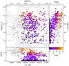 |
Fig. 14 sHR diagram of the stars in the sample color-coded by log Q. The bottom and right subpanels in each panel show this quantity against Teff and log ℒ, respectively. Cases in which log Q is degenerate are excluded (see Sect. 4.1). All panels include 191 O-type stars from Hol18-22 (gray circles). The evolutionary tracks are the same as in Fig. 7 for Geneva models. |
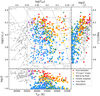 |
Fig. 15 Same as Fig. 14, but the color-coding represents the different shapes of the Hα line as classified in de Burgos et al. (2023, see also labels within the bottom right inset). |
6 Concluding remarks
We conducted a quantitative spectroscopic analysis of highresolution and high signal-to-noise optical spectra of 527 Galactic O9–B5 stars, collected from the IACOB spectroscopic database and the ESO public archive. The outcome of our analysis represents the most extensive collection of homogeneously determined spectroscopic parameters of Galactic BSG stars built to date, superseding previous attempts by more than one order of magnitude. This study aims to advance our understanding of the evolutionary nature of massive stars, also establishing new empirical anchor points for state-of-the-art and future model computations.
The spectroscopic analysis was carried out in two steps. First, we used IACOB-BROAD to derive the rotational and macroturbulent broadenings. Second, we used a suitable grid of model atmospheres computed with the FASTWIND code to create a statistical emulator for FASTWIND synthetic spectra. In combination with a Markov chain Monte Carlo method, we derived the fundamental atmospheric parameters, helium and silicon surface abundances, as well as an indicator of the wind strength.
We presented a revised calibration of Teff against spectral type for Galactic B-type supergiants down to B5-type stars. Previous calibrations based on smaller samples differ by up to 3 kK for some spectral-type bins when comparing a third-order polynomial fit to the data. Reliable spectral classifications from selected sources turned out to be crucial to avoid spurious results. In this latter regard, SIMBAD classifications for B-type stars exhibit inaccuracies, emphasizing the need for a systematic and reliable revision, similar to efforts in O-type star studies.
In comparison with the O-type stars, the relatively large number of early B-type supergiant stars included in our magnitude-limited sample suggest that at least a nonnegligible fraction of them could still be on the main sequence, in contrast to the classic interpretation that they are He-core burning post-MS objects. Our results present solid statistical evidence for a drastic drop in the relative number of objects at Teff ≈ 21 kK. Though further analyses are certainly required, we suggest that this drop (roughly occurring at B2-type stars) empirically locates the TAMS in the mass range between 15 and 85 M⊙.
Similarly to O-type stars, the distribution of projected rotational velocities for evolved B-type stars also exhibits two clear components: a low-υ sin i (< 100 km s−1) component that is present in the full range of covered effective temperatures, and a tail of fast rotators (reaching υ sin i values up to ≈400 km s−1) that disappears below ≈21 kK. Guided by some recent theoretical scenarios, our empirical study is consistent with the possibility that this tail of fast rotators is mostly populated by post-interaction binary products.
We observe no surface braking in the low-υ sin i component along the whole considered range of effective temperatures. This result, combined with a constant percentage of stars with υ sin i > 100 km s−1 and associated maximum υ sin i values from the ZAMS to the drop, might indicate the existence of a very efficient angular momentum transport mechanism between the core and the surface of massive stars.
The scarcity of stars populating the tail of fast rotators below Teff ≈ 21 kK has been attributed to either the end of the main sequence or the result of an enhanced angular momentum loss at the theoretically predicted bi-stability jump. Our combined results disfavor the latter scenario.
The distribution of ξ in the BSG domain is presented for the first time in an sHR diagram. A strong correlation between ξ and log ℒ is found. In agreement with previous findings, a decrease in both ξ and υmac toward lower Teff is also observed. This might indicate a connection between the physical mechanisms responsible for the two turbulent motions; our sample of stars supports higher ξ values to be associated with higher υmac.
Our findings for the helium surface abundance indicate that, on average, only ≈20% of luminous blue stars show helium enrichment (YHe > 0.13) in their atmospheres. No clear correlation is found between the surface abundance of helium and log ℒ or Teff. However, while we find a significantly lower percentage of He-enriched stars on the cooler side of the suggested empirical TAMS (Teff ≲ 20 kK), the percentage of He-enriched stars in the tail of fast rotators is systematically higher than for the main low-υ sin i component for stars with Teff above ≈20kK. In addition, we show with high statistical confidence that both groups of different υ sin i do not originate from the same probability distribution for the surface helium abundance, suggesting a different physical origin of the two populations. Compared with predictions from state-of-the-art evolutionary models, and considering the empirical evidence that the predicted surface braking might not occur, the possibility that He-enriched stars originate from single-star evolution seems less likely compared to a binary evolution origin.
Lastly, we evaluated the wind strength and its correlation with the morphology of the Hα profiles. Our results indicate no evidence of a mass-loss increase over the expected wind bi-stability region, but rather a slow decay of the maximum log Q values with decreasing Teff. We found a separation of stars with log Q above and below −13.6 in the Teff range below ≈22kK, each displaying a different Hα morphology. The presence of a positive correlation between log Q and log ℒ is also evident, where the highest values are concentrated at log(ℒ/ℒ⊙)) ≳ 3.9 dex. In general, we found a gradient of morphologies for Hα across the sHR diagram, with some profile shapes being concentrated in specific areas in the diagram.
As a final remark, the results presented here represent a significant step forward in the empirical spectroscopic study of Galactic luminous blue stars, providing an updated overview of many of their properties. These findings also lay the groundwork for forthcoming in-depth studies dedicated to specific properties of our sample. For this purpose, additional information is certainly required on luminosities, masses, radii, surface elemental abundances, and wind properties. Our ultimate objective is to establish new empirical anchor points that can serve to improve our understanding of the evolutionary nature of BSGs.
Acknowledgements
A.d.B. and S.S.-D. acknowledge support from the Spanish Ministry of Science and Innovation (MICINN) through the Spanish State Research Agency through grants PID2021-122397NB-C21, and the Severo Ochoa Programme 2020-2023 (CEX2019-000920-S). The authors would like to thank Z. Keszthelyi, D. Lennon, and N. Przybilla for their useful and valuable comments, and I. Negueruela for providing us with revised spectral classifications. We give special thanks to all the observers who contributed to the acquisition of the spectra used here in this work. Among them, especially to G. Holgado and J. Maíz-Apellániz. Regarding the observing facilities, this research is based on observations made with the Mercator Telescope, operated by the Flemish Community at the Observatorio del Roque de los Muchachos (La Palma, Spain), of the Instituto de Astrofísica de Canarias. In particular, obtained with the HERMES spectrograph, which is supported by the Research Foundation – Flanders (FWO), Belgium, the Research Council of KU Leuven, Belgium, the Fonds National de la Recherche Scientifique (F.R.S.-FNRS), Belgium, the Royal Observatory of Belgium, the Observatoire de Genève, Switzerland and the Thüringer Landessternwarte Tautenburg, Germany. This research also based on observations with the Nordic Optical Telescope, owned in collaboration by the University of Turku and Aarhus University, and operated jointly by Aarhus University, the University of Turku and the University of Oslo, representing Denmark, Finland and Norway, the University of Iceland and Stockholm University, at the Observatorio del Roque de los Muchachos, of the Instituto de Astrofísica de Canarias. Additionally, this work has made use of observations collected from the ESO Science Archive Facility under ESO programs: 60.A-9700(A), 72.D-0235(B), 73.C-0337(A), 73.D-0234(A), 73.D-0609(A), 74.D-0008(B), 74.D-0300(A), 75.D-0103(A), 75.D-0369(A), 76.C-0431(A), 77.D-0025(A), 77.D-0635(A), 79.A-9008(A), 79.B-0856(A), 81.A-9005(A), 81.A-9006(A), 81.C-2003(A), 81.D-2008(A), 81.D-2008(B), 82.D-0933(A), 83.D-0589(A), 83.D-0589(B), 85.D-0262(A), 86.D-0997(B), 87.D-0946(A), 88.A-9003(A), 89.D-0975(A), 90.D-0358(A), 91.C-0713(A), 91.D-0061(A), 91.D-0221(A), 92.A-9020(A), 95.A-9029(D), 97.A-9039(C), 102.A-9010(A) and 179.C-0197(C).
Appendix A Grid of input models
Figure A.1 displays an sHR diagram with the grid of 358 FASTWIND models used to train the statistical emulator which, as described in Sect. 3.2.2, is used to reproduce equivalent FASTWIND simulations. Figure A.2 illustrates the coverage of these models with respect to the remaining spectroscopic parameters.
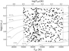 |
Fig. A.1 sHR diagram showing the initial grid of 358 FASTWIND computed models used in this work. The boundary limits are marked with dashed black lines. A set of Geneva nonrotating evolutionary tracks with solar metallicity is included for reference. |
 |
Fig. A.2 Same FASTWIND models as in Fig. A.1, but displaying the coverage of other stellar and wind parameters. |
Appendix B Visualization of the output solution
In Sect. 3.2, we described the method used to derive the best (i.e., most probable) set of parameters for each star. In each analysis, an associated synthetic spectrum is obtained, together with individual probability distributions of the parameters. An example of this output is included in Fig. B.1 for HD 198 478. The top array of subpanels shows the observed and synthetic spectra split into different windows that include the diagnostic lines listed in Table 2. The associated probability distributions are shown in the bottom grid of subpanels. Complementary to that figure, Fig. B.2 shows, for the same star, the probability distributions of the different parameters in a corner plot, allowing us to visualize the possible covariances. In this example, we see the (well-known) presence of a significant covariance between Teff and log 𝑔, arising from the behavior of the H-lines, as well as between β and log Q (see Markova et al. 2004). In addition, we can see that the distribution of the helium surface abundance reaches the lower boundary of the grid.
For each of the stellar and wind parameters, we also defined in Sect. 3.2.4 four possible scenarios for the associated probability distribution. Figure B.3 provides an example for each of the four possible cases described there.
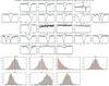 |
Fig. B.1 Summary of the analysis for HD 198478. The subpanels of the top five rows show the observed spectra (solid black line) and synthetic model (dashed green line) in different diagnostic windows used in the analysis of our sample. Within each window, the purple horizontal line indicates which subregions have not been masked in the analysis. The subpanels in the bottom two rows are the associated probability distributions of each of the parameters derived in this work. The vertical dashed red and orange lines indicate the maximum and median of the distribution and associated uncertainties. |
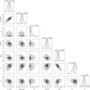 |
Fig. B.2 Corner plot with the PDFs of the seven parameters derived for HD 198 478. |
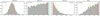 |
Fig. B.3 Illustrative example of the four different PDFs described in Sect. 3.2.4. From left to right: a well-behaved distribution (case a); an example of an undefined (degenerate) solution (d); and two cases for the upper and lower limits (c and b, respectively). |
Appendix C New spectral classifications
Table C.1 includes revisited spectral classifications based on visual morphological features for a group of stars erroneously classified as dwarfs in the default SIMBAD classification.
Appendix D Long tables
Results of the spectroscopic analysis of the stars in the sample (extract).
References
- Abbott, D. C. 1980, ApJ, 242, 1183 [NASA ADS] [CrossRef] [Google Scholar]
- Abbott, B. P., Abbott, R., Abbott, T. D., et al. 2016, Phys. Rev. Lett., 116, 061102 [Google Scholar]
- Aerts, C., & Rogers, T. M. 2015, ApJ, 806, L33 [Google Scholar]
- Aerts, C., Puls, J., Godart, M., & Dupret, M. A. 2009, A&A, 508, 409 [NASA ADS] [CrossRef] [EDP Sciences] [Google Scholar]
- Anders, E. H., Lecoanet, D., Cantiello, M., et al. 2023, Nat. Astron., 7, 1228 [NASA ADS] [CrossRef] [Google Scholar]
- Asplund, M., Grevesse, N., Sauval, A. J., & Scott, P. 2009, ARA&A, 47, 481 [NASA ADS] [CrossRef] [Google Scholar]
- Belczynski, K., Holz, D. E., Bulik, T., & O’Shaughnessy, R. 2016, Nature, 534, 512 [NASA ADS] [CrossRef] [Google Scholar]
- Bernini-Peron, M., Marcolino, W. L. F., Sander, A. A. C., et al. 2023, A&A, 677, A50 [NASA ADS] [CrossRef] [EDP Sciences] [Google Scholar]
- Björklund, R., Sundqvist, J. O., Puls, J., & Najarro, F. 2021, A&A, 648, A36 [EDP Sciences] [Google Scholar]
- Björklund, R., Sundqvist, J. O., Singh, S. M., Puls, J., & Najarro, F. 2023, A&A, 676, A109 [NASA ADS] [CrossRef] [EDP Sciences] [Google Scholar]
- Bowman, D. M., Aerts, C., Johnston, C., et al. 2019a, A&A, 621, A135 [NASA ADS] [CrossRef] [EDP Sciences] [Google Scholar]
- Bowman, D. M., Burssens, S., Pedersen, M. G., et al. 2019b, Nat. Astron., 3, 760 [Google Scholar]
- Bowman, D. M., Burssens, S., Simón-Díaz, S., et al. 2020, A&A, 640, A36 [NASA ADS] [CrossRef] [EDP Sciences] [Google Scholar]
- Brands, S. A., de Koter, A., Bestenlehner, J. M., et al. 2022, A&A, 663, A36 [Google Scholar]
- Bresolin, F., Urbaneja, M. A., Gieren, W., Pietrzynski, G., & Kudritzki, R.-P. 2007, ApJ, 671, 2028 [NASA ADS] [CrossRef] [Google Scholar]
- Bresolin, F., Kudritzki, R.-P., Urbaneja, M. A., et al. 2016, ApJ, 830, 64 [NASA ADS] [CrossRef] [Google Scholar]
- Bresolin, F., Kudritzki, R.-P., & Urbaneja, M. A. 2022, ApJ, 940, 32 [NASA ADS] [CrossRef] [Google Scholar]
- Britavskiy, N., Simón-Díaz, S., Holgado, G., et al. 2023, A&A, 672, A22 [NASA ADS] [CrossRef] [EDP Sciences] [Google Scholar]
- Brott, I., de Mink, S. E., Cantiello, M., et al. 2011, A&A, 530, A115 [NASA ADS] [CrossRef] [EDP Sciences] [Google Scholar]
- Butler, K., & Giddings, J. 1985, Newsletter on the analysis of astronomical spectra No. 9, College London [Google Scholar]
- Cantiello, M., Langer, N., Brott, I., et al. 2009, A&A, 499, 279 [NASA ADS] [CrossRef] [EDP Sciences] [Google Scholar]
- Cantiello, M., Lecoanet, D., Jermyn, A. S., & Grassitelli, L. 2021, ApJ, 915, 112 [NASA ADS] [CrossRef] [Google Scholar]
- Carneiro, L. P., Puls, J., Sundqvist, J. O., & Hoffmann, T. L. 2016, A&A, 590, A88 [NASA ADS] [CrossRef] [EDP Sciences] [Google Scholar]
- Castro, N., Fossati, L., Langer, N., et al. 2014, A&A, 570, A13 [NASA ADS] [CrossRef] [EDP Sciences] [Google Scholar]
- Chib, S. 2001, in Handbook of Econometrics, 5, Markov Chain Monte Carlo Methods: Computation and Inference, Chapter 57, eds. J. J. Heckman & E. Leamer (Elsevier), 3569 [Google Scholar]
- Conti, P. S., & Ebbets, D. 1977, ApJ, 213, 438 [CrossRef] [Google Scholar]
- Crowther, P. A., Lennon, D. J., & Walborn, N. R. 2006, A&A, 446, 279 [NASA ADS] [CrossRef] [EDP Sciences] [Google Scholar]
- de Burgos, A., Simon-Díaz, S., Lennon, D. J., et al. 2020, A&A, 643, A116 [NASA ADS] [CrossRef] [EDP Sciences] [Google Scholar]
- de Burgos, A., Simón-Díaz, S., Urbaneja, M. A., & Negueruela, I. 2023, A&A, 674, A212 [NASA ADS] [CrossRef] [EDP Sciences] [Google Scholar]
- de Mink, S. E., Langer, N., Izzard, R. G., Sana, H., & de Koter, A. 2013, ApJ, 764, 166 [Google Scholar]
- Dufton, P. L. 1972, A&A, 16, 301 [NASA ADS] [Google Scholar]
- Edelmann, P. V. F., Ratnasingam, R. P., Pedersen, M. G., et al. 2019, ApJ, 876, 4 [NASA ADS] [CrossRef] [Google Scholar]
- Ekström, S., Georgy, C., Eggenberger, P., et al. 2012, A&A, 537, A146 [Google Scholar]
- Fitzpatrick, E. L., & Garmany, C. D. 1990, ApJ, 363, 119 [Google Scholar]
- Fraser, M., Dufton, P. L., Hunter, I., & Ryans, R. S. I. 2010, MNRAS, 404, 1306 [NASA ADS] [Google Scholar]
- Geen, S., Bieri, R., Rosdahl, J., & de Koter, A. 2021, MNRAS, 501, 1352 [Google Scholar]
- Georgy, C., Ekström, S., Eggenberger, P., et al. 2013, A&A, 558, A103 [NASA ADS] [CrossRef] [EDP Sciences] [Google Scholar]
- Georgy, C., Saio, H., & Meynet, G. 2021, A&A, 650, A128 [NASA ADS] [CrossRef] [EDP Sciences] [Google Scholar]
- Giddings, J. R. 1981, PhD thesis, University of London [Google Scholar]
- Gies, D. R., & Lambert, D. L. 1992, ApJ, 387, 673 [Google Scholar]
- Glebbeek, E., Gaburov, E., Portegies Zwart, S., & Pols, O. R. 2013, MNRAS, 434, 3497 [NASA ADS] [CrossRef] [Google Scholar]
- Godart, M., Simón-Díaz, S., Herrero, A., et al. 2017, A&A, 597, A23 [NASA ADS] [CrossRef] [EDP Sciences] [Google Scholar]
- Gräfener, G., Koesterke, L., & Hamann, W. R. 2002, A&A, 387, 244 [NASA ADS] [CrossRef] [EDP Sciences] [Google Scholar]
- Grassitelli, L., Fossati, L., Simón-Diáz, S., et al. 2015, ApJ, 808, L31 [NASA ADS] [CrossRef] [Google Scholar]
- Grin, N. J., Ramírez-Agudelo, O. H., de Koter, A., et al. 2017, A&A, 600, A82 [NASA ADS] [CrossRef] [EDP Sciences] [Google Scholar]
- Hamann, W. R., & Gräfener, G. 2004, A&A, 427, 697 [NASA ADS] [CrossRef] [EDP Sciences] [Google Scholar]
- Haucke, M., Cidale, L. S., Venero, R. O. J., et al. 2018, A&A, 614, A91 [NASA ADS] [CrossRef] [EDP Sciences] [Google Scholar]
- Hauschildt, P. H. 1992, J. Quant. Spec. Radiat. Transf., 47, 433 [NASA ADS] [CrossRef] [Google Scholar]
- Hawcroft, C., Sana, H., Marry, L., et al. 2021, A&A, 655, A67 [NASA ADS] [CrossRef] [EDP Sciences] [Google Scholar]
- Hayashi, C., & Cameron, R. C. 1962, ApJ, 136, 166 [CrossRef] [Google Scholar]
- Hillier, D. J., & Miller, D. L. 1998, ApJ, 496, 407 [NASA ADS] [CrossRef] [Google Scholar]
- Holgado, G. 2019, PhD thesis, Astrophysical Institute of the Canaries; University of La Laguna, Spain [Google Scholar]
- Holgado, G., Simón-Díaz, S., Barbá, R. H., et al. 2018, A&A, 613, A65 [NASA ADS] [CrossRef] [EDP Sciences] [Google Scholar]
- Holgado, G., Simón-Díaz, S., Haemmerlé, L., et al. 2020, A&A, 638, A157 [NASA ADS] [CrossRef] [EDP Sciences] [Google Scholar]
- Holgado, G., Simón-Díaz, S., Herrero, A., & Barbá, R. H. 2022, A&A, 665, A150 [NASA ADS] [CrossRef] [EDP Sciences] [Google Scholar]
- Howarth, I. D., Siebert, K. W., Hussain, G. A. J., & Prinja, R. K. 1997, MNRAS, 284, 265 [NASA ADS] [CrossRef] [Google Scholar]
- Hubeny, I. 1988, Comput. Phys. Commun., 52, 103 [Google Scholar]
- Hunter, I., Dufton, P. L., Smartt, S. J., et al. 2007, A&A, 466, 277 [NASA ADS] [CrossRef] [EDP Sciences] [Google Scholar]
- Hunter, I., Lennon, D. J., Dufton, P. L., et al. 2008, A&A, 479, 541 [NASA ADS] [CrossRef] [EDP Sciences] [Google Scholar]
- Hunter, I., Brott, I., Langer, N., et al. 2009, A&A, 496, 841 [NASA ADS] [CrossRef] [EDP Sciences] [Google Scholar]
- Kaufer, A., Wolf, B., Andersen, J., & Pasquini, L. 1997, The Messenger, 89, 1 [NASA ADS] [Google Scholar]
- Keszthelyi, Z., Meynet, G., Georgy, C., et al. 2019, MNRAS, 485, 5843 [NASA ADS] [CrossRef] [Google Scholar]
- Keszthelyi, Z., de Koter, A., Götberg, Y., et al. 2022, MNRAS, 517, 2028 [Google Scholar]
- Kim, J.-G., Kim, W.-T., & Ostriker, E. C. 2019, ApJ, 883, 102 [Google Scholar]
- Klencki, J., Nelemans, G., Istrate, A. G., & Pols, O. 2020, A&A, 638, A55 [NASA ADS] [CrossRef] [EDP Sciences] [Google Scholar]
- Krause, M., Fierlinger, K., Diehl, R., et al. 2013, A&A, 550, A49 [NASA ADS] [CrossRef] [EDP Sciences] [Google Scholar]
- Krtička, J., Kubát, J., & Krticková, I. 2024, A&A, 681, A29 [NASA ADS] [CrossRef] [EDP Sciences] [Google Scholar]
- Kudritzki, R.-P., & Przybilla, N. 2003, in Stellar Candles for the Extragalac-tic Distance Scale, 635, eds. D. Alloin, & W. Gieren (Springer Berlin Heidelberg), 123 [NASA ADS] [CrossRef] [Google Scholar]
- Kudritzki, R.-P., Urbaneja, M. A., Bresolin, F., et al. 2008, ApJ, 681, 269 [NASA ADS] [CrossRef] [Google Scholar]
- Kudritzki, R.-P., Urbaneja, M. A., Gazak, Z., et al. 2012, ApJ, 747, 15 [CrossRef] [Google Scholar]
- Kurucz, R. L. 2005, Mem. Soc. Astron. Ital. Suppl., 8, 14 [Google Scholar]
- Langer, N. 2012, ARA&A, 50, 107 [CrossRef] [Google Scholar]
- Langer, N., & Kudritzki, R. P. 2014, A&A, 564, A52 [NASA ADS] [CrossRef] [EDP Sciences] [Google Scholar]
- Langer, N., Schürmann, C., Stoll, K., et al. 2020, A&A, 638, A39 [NASA ADS] [CrossRef] [EDP Sciences] [Google Scholar]
- Lecoanet, D., & Edelmann, P. V. F. 2023, Galaxies, 11, 89 [NASA ADS] [CrossRef] [Google Scholar]
- Lefever, K., Puls, J., & Aerts, C. 2007, A&A, 463, 1093 [NASA ADS] [CrossRef] [EDP Sciences] [Google Scholar]
- Lennon, D. J., Dufton, P. L., & Fitzsimmons, A. 1992, A&AS, 94, 569 [NASA ADS] [Google Scholar]
- Mackay, D. J. C. 2003, Information Theory, Inference and Learning Algorithms (Cambridge University Press) [Google Scholar]
- Maeder, A. 1981, A&A, 101, 385 [NASA ADS] [Google Scholar]
- Maeder, A., & Meynet, G. 2005, A&A, 440, 1041 [NASA ADS] [CrossRef] [EDP Sciences] [Google Scholar]
- Maeder, A., & Meynet, G. 2012, Rev. Mod. Phys., 84, 25 [Google Scholar]
- Magg, E., Bergemann, M., Serenelli, A., et al. 2022, A&A, 661, A140 [NASA ADS] [CrossRef] [EDP Sciences] [Google Scholar]
- Maíz Apellániz, J., Sota, A., Walborn, N. R., et al. 2011, in Highlights of Spanish Astrophysics VI, eds. M. R. Zapatero Osorio, J. Gorgas, J. Maíz Apellániz, J. R. Pardo, & A. Gil de Paz, 467 [Google Scholar]
- Maíz Apellániz, J., Sota, A., Arias, J. I., et al. 2016, ApJS, 224, 4 [CrossRef] [Google Scholar]
- Marchant, P., & Bodensteiner, J. 2023, arXiv e-prints [arXiv:2311.01865] [Google Scholar]
- Marchant, P., Langer, N., Podsiadlowski, P., Tauris, T. M., & Moriya, T. J. 2016, A&A, 588, A50 [NASA ADS] [CrossRef] [EDP Sciences] [Google Scholar]
- Markova, N., & Puls, J. 2008, A&A, 478, 823 [NASA ADS] [CrossRef] [EDP Sciences] [Google Scholar]
- Markova, N., Puls, J., Repolust, T., & Markov, H. 2004, A&A, 413, 693 [NASA ADS] [CrossRef] [EDP Sciences] [Google Scholar]
- Martinet, S., Meynet, G., Ekström, S., et al. 2021, A&A, 648, A126 [NASA ADS] [CrossRef] [EDP Sciences] [Google Scholar]
- Martins, F., Schaerer, D., & Hillier, D. J. 2005, A&A, 436, 1049 [NASA ADS] [CrossRef] [EDP Sciences] [Google Scholar]
- McErlean, N. D., Lennon, D. J., & Dufton, P. L. 1998, A&A, 329, 613 [NASA ADS] [Google Scholar]
- McErlean, N. D., Lennon, D. J., & Dufton, P. L. 1999, A&A, 349, 553 [NASA ADS] [Google Scholar]
- McEvoy, C. M., Dufton, P. L., Evans, C. J., et al. 2015, A&A, 575, A70 [NASA ADS] [CrossRef] [EDP Sciences] [Google Scholar]
- McKay, M. D., Beckman, R. J., & Conover, W. J. 1979, Technometrics, 21, 239 [Google Scholar]
- Menon, A., Ercolino, A., Urbaneja, M. A., et al. 2023, arXiv e-prints [arXiv:2311.05581] [Google Scholar]
- Metropolis, N., Rosenbluth, A. W., Rosenbluth, M. N., Teller, A. H., & Teller, E. 1953, J. Chem. Phys., 21, 1087 [Google Scholar]
- Meynet, G., & Maeder, A. 2000, A&A, 361, 101 [NASA ADS] [Google Scholar]
- Najarro, F., Hanson, M. M., & Puls, J. 2011, A&A, 535, A32 [NASA ADS] [CrossRef] [EDP Sciences] [Google Scholar]
- Negueruela, I. 2004, Astron. Nachr., 325, 380 [Google Scholar]
- Negueruela, I., Simón-Díaz, S., de Burgos, A., Casabuenas, A., & Beck, P. 2024 A&A, submitted [NASA ADS] [CrossRef] [EDP Sciences] [Google Scholar]
- Nieva, M. F., & Przybilla, N. 2012, A&A, 539, A143 [NASA ADS] [CrossRef] [EDP Sciences] [Google Scholar]
- Nomoto, K., Kobayashi, C., & Tominaga, N. 2013, ARA&A, 51, 457 [CrossRef] [Google Scholar]
- Pauldrach, A. W. A., & Puls, J. 1990, A&A, 237, 409 [NASA ADS] [Google Scholar]
- Pauldrach, A., Puls, J., & Kudritzki, R. P. 1986, A&A, 164, 86 [NASA ADS] [Google Scholar]
- Pauldrach, A. W. A., Hoffmann, T. L., & Lennon, M. 2001, A&A, 375, 161 [NASA ADS] [CrossRef] [EDP Sciences] [Google Scholar]
- Petrov, B., Vink, J. S., & Gräfener, G. 2016, MNRAS, 458, 1999 [NASA ADS] [CrossRef] [Google Scholar]
- Podsiadlowski, P., Joss, P. C., & Hsu, J. J. L. 1992, ApJ, 391, 246 [Google Scholar]
- Puls, J., Kudritzki, R. P., Herrero, A., et al. 1996, A&A, 305, 171 [Google Scholar]
- Puls, J., Urbaneja, M. A., Venero, R., et al. 2005, A&A, 435, 669 [NASA ADS] [CrossRef] [EDP Sciences] [Google Scholar]
- Puls, J., Vink, J. S., & Najarro, F. 2008, A&A Rev., 16, 209 [NASA ADS] [CrossRef] [Google Scholar]
- Puls, J., Najarro, F., Sundqvist, J. O., & Sen, K. 2020, A&A, 642, A172 [EDP Sciences] [Google Scholar]
- Rivero González, J. G., Puls, J., & Najarro, F. 2011, A&A, 536, A58 [NASA ADS] [CrossRef] [EDP Sciences] [Google Scholar]
- Rivero González, J. G., Puls, J., Massey, P., & Najarro, F. 2012, A&A, 543, A95 [NASA ADS] [CrossRef] [EDP Sciences] [Google Scholar]
- Ryans, R. S. I., Dufton, P. L., Rolleston, W. R. J., et al. 2002, MNRAS, 336, 577 [Google Scholar]
- Santolaya-Rey, A. E., Puls, J., & Herrero, A. 1997, A&A, 323, 488 [NASA ADS] [Google Scholar]
- Schneider, F. R. N., Podsiadlowski, P., Langer, N., Castro, N., & Fossati, L. 2016, MNRAS, 457, 2355 [Google Scholar]
- Schootemeijer, A., Langer, N., Grin, N. J., & Wang, C. 2019, A&A, 625, A132 [NASA ADS] [CrossRef] [EDP Sciences] [Google Scholar]
- Scott, L. J. A., Hirschi, R., Georgy, C., et al. 2021, MNRAS, 503, 4208 [NASA ADS] [CrossRef] [Google Scholar]
- Searle, S. C., Prinja, R. K., Massa, D., & Ryans, R. 2008, A&A, 481, 777 [NASA ADS] [CrossRef] [EDP Sciences] [Google Scholar]
- Sen, K., Langer, N., Marchant, P., et al. 2022, A&A, 659, A98 [NASA ADS] [CrossRef] [EDP Sciences] [Google Scholar]
- Simón-Díaz, S., & Herrero, A. 2014, A&A, 562, A135 [NASA ADS] [CrossRef] [EDP Sciences] [Google Scholar]
- Simón-Díaz, S., Herrero, A., Uytterhoeven, K., et al. 2010, ApJ, 720, L174 [CrossRef] [Google Scholar]
- Simón-Díaz, S., Herrero, A., Sabín-Sanjulián, C., et al. 2014, A&A, 570, A6 [NASA ADS] [CrossRef] [EDP Sciences] [Google Scholar]
- Simón-Díaz, S., Godart, M., Castro, N., et al. 2017, A&A, 597, A22 [CrossRef] [EDP Sciences] [Google Scholar]
- Simón-Díaz, S., Pérez Prieto, J. A., Holgado, G., de Burgos, A., & Iacob Team 2020, in XIV.0 Scientific Meeting (virtual) of the Spanish Astronomical Society, 187 [Google Scholar]
- Smartt, S. J. 2009, ARA&A, 47, 63 [NASA ADS] [CrossRef] [Google Scholar]
- Smith, K. C., & Howarth, I. D. 1998, MNRAS, 299, 1146 [Google Scholar]
- Sota, A., Maíz Apellániz, J., Walborn, N. R., et al. 2011, ApJS, 193, 24 [Google Scholar]
- Sota, A., Maiz Apellaniz, J., Walborn, N. R., et al. 2014, VizieR Online Data Catalog: III/274 [Google Scholar]
- Stothers, R., & Chin, C. W. 1975, ApJ, 198, 407 [NASA ADS] [CrossRef] [Google Scholar]
- Sundqvist, J. O., & Puls, J. 2018, A&A, 619, A59 [NASA ADS] [CrossRef] [EDP Sciences] [Google Scholar]
- Taormina, M., Kudritzki, R.-P., Puls, J., et al. 2020, ApJ, 890, 137 [NASA ADS] [CrossRef] [Google Scholar]
- Urbaneja, M. A., Herrero, A., Bresolin, F., et al. 2003, ApJ, 584, L73 [Google Scholar]
- Urbaneja, M. A., Herrero, A., Bresolin, F., et al. 2005a, ApJ, 622, 862 [Google Scholar]
- Urbaneja, M. A., Herrero, A., Kudritzki, R. P., et al. 2005b, ApJ, 635, 311 [NASA ADS] [CrossRef] [Google Scholar]
- Urbaneja, M. A., Herrero, A., Lennon, D. J., Corral, L. J., & Meynet, G. 2011, ApJ, 735, 39 [NASA ADS] [CrossRef] [Google Scholar]
- Urbaneja, M. A., Kudritzki, R. P., Gieren, W., et al. 2017, AJ, 154, 102 [NASA ADS] [CrossRef] [Google Scholar]
- Vink, J. S., de Koter, A., & Lamers, H. J. G. L. M. 1999, A&A, 350, 181 [NASA ADS] [Google Scholar]
- Vink, J. S., de Koter, A., & Lamers, H. J. G. L. M. 2000, A&A, 362, 295 [NASA ADS] [Google Scholar]
- Vink, J. S., Brott, I., Gräfener, G., et al. 2010, A&A, 512, A7 [NASA ADS] [CrossRef] [EDP Sciences] [Google Scholar]
- Wang, C., Langer, N., Schootemeijer, A., et al. 2020, ApJ, 888, L12 [NASA ADS] [CrossRef] [Google Scholar]
- Watkins, E. J., Peretto, N., Marsh, K., & Fuller, G. A. 2019, A&A, 628, A21 [NASA ADS] [CrossRef] [EDP Sciences] [Google Scholar]
- Wei-Liem, L. 1996, Ann. Statist., 24, 2058 [Google Scholar]
- Weis, K., & Bomans, D. J. 2020, Galaxies, 8, 20 [NASA ADS] [CrossRef] [Google Scholar]
- Wenger, M., Ochsenbein, F., Egret, D., et al. 2000, A&AS, 143, 9 [NASA ADS] [CrossRef] [EDP Sciences] [Google Scholar]
- Weßmayer, D., Przybilla, N., & Butler, K. 2022, A&A, 668, A92 [NASA ADS] [CrossRef] [EDP Sciences] [Google Scholar]
- Woosley, S. E., & Weaver, T. A. 1995, ApJS, 101, 181 [Google Scholar]
- Woosley, S. E., & Bloom, J. S. 2006, ARA&A, 44, 507 [Google Scholar]
- Zhao, L., Song, H., Meynet, G., et al. 2023, A&A, 674, A92 [NASA ADS] [CrossRef] [EDP Sciences] [Google Scholar]
See Table D.1 for information about the spectral classifications adopted in this work.
For all lines from the so-called explicit elements that are used for the analysis (here hydrogen, helium, and silicon), as well as for the strongest lines from other elements (in between C and Zn); most other lines are treated within the Sobolev approximation.
Q is defined as Ṁ/(R⋆υ∞)1.5 (see Puls et al. 1996, 2005).
In particular: 1000K in Teff, 0.1 dex in log 𝑔, 5 km s–1 in ξ, 0.04 in YHe, 0.15 in ϵSi, 0.3 in log Q, and 0.7 in β.
For example, the case shown in the bottom panel of Fig. 4, which corresponds to the X-ray binary system HD226 868 (Cyg-X1) an O9.7Iab star orbiting a black hole.
The proposed location of the bi-stability jump in Vink et al. (2000) for the range of luminosities of the considered BSGs is ≈25 kK.
Here derived adopting an unclumped wind; however, when replacing Ṁ by  in the definition of Q (with fcl the conventional clumping factor for optically thin clumping), the Q-values derived in this work remain roughly valid also for inhomogeneous winds.8
All Tables
Parameter space covered by the model atmosphere calculations used in the present work.
List of diagnostic lines used for the determination of the spectroscopic parameters.
Summary properties of He-enriched stars, separated in groups of different Teff and log(ℒ/ℒ⊙), as indicated in the second and third columns.
All Figures
|
Fig. 1 Some illustrative examples of spectra used in this work, ordered by spectral type. Three different spectral windows depict the wavelength ranges in which the main diagnostic lines used to obtain estimates of the spectroscopic parameters are located. The vertical red, cyan, and brown bars indicate the corresponding H I, He I–II, and Si II–III–IV lines (see Sect. 3.2.3 for further details). |
| In the text | |
|
Fig. 2 Examples of different masks used to select the diagnostic lines. Each of the four panels shows the same wavelength range including the He II λ4542 Å line and the Si III λλ4553,4568,4575 Å triplet. The two panels on the left compare two stars of similar temperature but different υ sin i: HD 14 302 with υ sin i ≈ 65 km s−1 (top left), and HD 197 460 with υ sin i ≈ 200 km s−1 (bottom left). The two panels on the right compare two stars of similar υ sin i but very different Teff : HD 24 432 with Teff = 15 kK (top right) and HD 190991 with Teff =32kK (bottom right). The wavelength ranges selected for each analysis are shaded in green. The masked (not used) regions are shaded in red. |
| In the text | |
|
Fig. 3 Histograms of the five quality indicators described in Sect. 3.2.5, each connected to a physical property, as indicated in the label of each panel. All histograms combine the information of all the stars with reliable estimates of Teff and log 𝑔. The gray bins correspond to values within 3-σ after applying an iterative clipping until convergence is achieved, while the red bins correspond to the clipped values. The median and 3-σ values are indicated in the figure with vertical and dash-dotted blue lines, respectively. The associated values are shown in the legend. For the panel associated with the wind strength, the x-axis extends to significantly higher values than for the others. |
| In the text | |
|
Fig. 4 Four illustrative cases of the quality labels assigned to the solutions (see text). Each row is divided into three spectral windows presenting three of the diagnostic regions: Si III λλ4553–68–75 triplet (left); He I λ4471 (middle); and Hα (right). The dashed green line is the synthetic spectrum of the model with the best-fitting parameters; the solid black line is the observed spectrum. |
| In the text | |
|
Fig. 5 Comparison of the results of the Teff and log 𝑔 with previous studies in the literature. The acronyms follow those used in Table 4. The error bars in the bottom right corners indicate the average uncertainty from our analysis (vertical axis) or from the literature (horizontal axis) except for those from Weßmayer et al. (2022) for which a separate error bar in pink is included. The two shaded areas indicate a difference in Teff and log 𝑔 of 1000 K and 0.1 dex, and 2000 K and 0.2 dex, respectively. The diagonal black line indicates the 1-to-1 agreement. |
| In the text | |
|
Fig. 6 Teff against spectral type for stars with luminosity class I. The blue dots correspond to stars with revised classifications (see Sect. 4.3), whereas the gray dots correspond to stars whose classification corresponds to the default provided by SIMBAD. The dashed orange and cyan lines correspond to a first- and third-order polynomial fit to the stars in blue. Some previous calibrations from the literature are also included for comparison. |
| In the text | |
|
Fig. 7 sHR diagram showing our results from the analysis for 527 stars with O9–B5 spectral type color-coded by their luminosity class, and 191 O-type stars from Hol18-22 in gray. The boundaries of our model grid are indicated with a rectangle. The shaded area indicates the approximate region where our results correspond to the upper or lower limits (see Sect. 3.2.4). The approximate separation between the O- and B-type stars is indicated with a dotted diagonal black line. For reference, the figure includes nonrotating evolutionary tracks with solar metallicity from the Geneva and Bonn models (Ekström et al. 2012; Georgy et al. 2013; Brott et al. 2011, respectively). Intervals of the same age difference are marked with purple crosses for Geneva and green triangles for Bonn, which are connected with dashed and dash-dotted lines of the same color. The dash-dotted gray lines indicate different constant log g values. |
| In the text | |
|
Fig. 8 Histogram of effective temperatures for all the stars in Fig. 7, color-coded by luminosity class. The approximate separation between O- and B-type stars is indicated with a dashed vertical black line. |
| In the text | |
|
Fig. 9 sHR diagram of the 527 stars in the sample and 191 O-type stars from Hol18-22, all color-coded by v sin i. The bottom and right subpanels show υ sin i against Teff and log ℒ, respectively. The boundary limits of our grid of models are marked with dashed black lines. The evolutionary tracks are the same as in Fig. 7 for Geneva models. |
| In the text | |
|
Fig. 10 Distribution of υ sin i separating the stars in the sample in four groups of different Teff ranges, as shown in the legends. The panels show the different histograms, indicating with a dash-dotted line the mean υ sin i values as derived from an iterative 2-σ clipping. In each panel the corresponding cumulative distribution and the percentage of stars with υ sin i < 100 km s−1 is also included. |
| In the text | |
|
Fig. 11 sHR diagram of the stars in the sample color-coded by the ξ. The bottom and right subpanels show ξ against Teff and log ℒ, respectively. Results of ξ considered as upper or lower limits, or degenerated are excluded. The evolutionary tracks are the same as in Fig. 7 for Geneva models. |
| In the text | |
|
Fig. 12 Macroturbulence against microturbulence for the sample of stars, color-coded by their log(ℒ/ℒ⊙). The sample is limited to those stars with υ sin i < 100 km s−1. A linear fit is included and is indicated by a dashed diagonal black line. |
| In the text | |
|
Fig. 13 sHR diagram of the stars in the sample plus 191 O-type stars from Hol18-22, color-coded by helium abundance. We adopted YHe ≈ 0.10 as the lowest possible value. The bottom and right subpanels show YHe against Teff and log ℒ, respectively. The various subgroups of stars listed in Table 5 are indicated with red solid lines. Results considered as lower limits or degenerate are excluded. The bottom subpanel includes a horizontal dotted line at YHe =0.13. The evolutionary tracks are the same as in Fig. 7 for Geneva models. |
| In the text | |
|
Fig. 14 sHR diagram of the stars in the sample color-coded by log Q. The bottom and right subpanels in each panel show this quantity against Teff and log ℒ, respectively. Cases in which log Q is degenerate are excluded (see Sect. 4.1). All panels include 191 O-type stars from Hol18-22 (gray circles). The evolutionary tracks are the same as in Fig. 7 for Geneva models. |
| In the text | |
|
Fig. 15 Same as Fig. 14, but the color-coding represents the different shapes of the Hα line as classified in de Burgos et al. (2023, see also labels within the bottom right inset). |
| In the text | |
|
Fig. A.1 sHR diagram showing the initial grid of 358 FASTWIND computed models used in this work. The boundary limits are marked with dashed black lines. A set of Geneva nonrotating evolutionary tracks with solar metallicity is included for reference. |
| In the text | |
|
Fig. A.2 Same FASTWIND models as in Fig. A.1, but displaying the coverage of other stellar and wind parameters. |
| In the text | |
|
Fig. B.1 Summary of the analysis for HD 198478. The subpanels of the top five rows show the observed spectra (solid black line) and synthetic model (dashed green line) in different diagnostic windows used in the analysis of our sample. Within each window, the purple horizontal line indicates which subregions have not been masked in the analysis. The subpanels in the bottom two rows are the associated probability distributions of each of the parameters derived in this work. The vertical dashed red and orange lines indicate the maximum and median of the distribution and associated uncertainties. |
| In the text | |
|
Fig. B.2 Corner plot with the PDFs of the seven parameters derived for HD 198 478. |
| In the text | |
|
Fig. B.3 Illustrative example of the four different PDFs described in Sect. 3.2.4. From left to right: a well-behaved distribution (case a); an example of an undefined (degenerate) solution (d); and two cases for the upper and lower limits (c and b, respectively). |
| In the text | |
Current usage metrics show cumulative count of Article Views (full-text article views including HTML views, PDF and ePub downloads, according to the available data) and Abstracts Views on Vision4Press platform.
Data correspond to usage on the plateform after 2015. The current usage metrics is available 48-96 hours after online publication and is updated daily on week days.
Initial download of the metrics may take a while.