| Issue |
A&A
Volume 681, January 2024
|
|
|---|---|---|
| Article Number | A1 | |
| Number of page(s) | 17 | |
| Section | Numerical methods and codes | |
| DOI | https://doi.org/10.1051/0004-6361/202346814 | |
| Published online | 20 December 2023 | |
Separation of dust emission from the cosmic infrared background in Herschel observations with wavelet phase harmonics
1
Laboratoire de Physique de l’École normale supérieure, ENS, Université PSL, CNRS, Sorbonne Université, Université Paris Cité,
75005
Paris,
France
e-mail: This email address is being protected from spambots. You need JavaScript enabled to view it.
2
Aix Marseille Univ, CNRS, LAM, Laboratoire d’Astrophysique de Marseille,
Marseille,
France
3
Canadian Institute for Theoretical Astrophysics, University of Toronto,
60 St. George Street,
Toronto,
ON M5S 3H8,
Canada
4
Research School of Astronomy & Astrophysics, Autralian National University,
Cambera, ACT,
2610
Australia
5
Institut d’Astrophysique Spatiale, Université Paris-Sud,
Bât. 121,
91405
Orsay,
France
6
Center for Computational Mathematics, Flatiron Institute,
162 5th Avenue,
New York, NY
10010,
USA
Received:
4
May
2023
Accepted:
23
October
2023
Abstract
The low-brightness dust emission at high Galactic latitudes is of interest with respect to studying the interplay among the physical processes involved in shaping the structure of the interstellar medium (ISM), as well as in statistical characterizations of the dust emission as a foreground to the cosmic microwave background (CMB). Progress in this avenue of research has been hampered by the difficulty related to separating the dust emission from the cosmic infrared background (CIB). We demonstrate that the dust and CIB may be effectively separated based on their different structure on the sky and we use the separation to characterize the structure of diffuse dust emission on angular scales, where the CIB is a significant component in terms of power. We used scattering transform statistics, wavelet phase harmonics (WPH) to perform a statistical component separation using Herschel SPIRE observations. This component separation is done only from observational data using non-Gaussian properties as a lever arm and is done at a single 250 µm frequency. This method, which we validated on mock data, gives us access to non-Gaussian statistics of the interstellar dust and an output dust map that is essentially free from CIB contamination. Our statistical modeling characterizes the non-Gaussian structure of the diffuse ISM down to the smallest scales observed by Herschel. We recovered the power law shape of the dust power spectrum up to k = 2 arcmin−1, where the dust signal represents 2% of the total power. Going beyond the standard power spectra analysis, we show that the non-Gaussian properties of the dust emission are not scale-invariant. The output dust map reveals coherent structures at the smallest scales, which had been hidden by the CIB anisotropies. This aspect opens up new observational perspectives on the formation of structure in the diffuse ISM, which we discuss here in reference to a previous work. We have succeeded in performing a statistical separation from the observational data at a single frequency by using non-Gaussian statistics.
Key words: methods: statistical / dust, extinction / infrared: diffuse background
© The Authors 2023
 Open Access article, published by EDP Sciences, under the terms of the Creative Commons Attribution License (https://creativecommons.org/licenses/by/4.0), which permits unrestricted use, distribution, and reproduction in any medium, provided the original work is properly cited.
This article is published in open access under the Subscribe to Open model. This email address is being protected from spambots. You need JavaScript enabled to view it. to support open access publication.
1 Introduction
Thermal emission from interstellar dust and the cosmic infrared background (CIB) are the two main emission components of the sky at far-infrared and sub-millimeter wavelengths. The emission from dust is a tracer of diffuse interstellar matter imaged for the first time across the sky by the IRAS space mission (Gautier et al. 1992; Miville-Deschênes et al. 2007). More recently, the Herschel space mission has provided data at a higher angular resolution, which are useful in characterizing the filamentary structure of molecular clouds (André et al. 2010; Miville-Deschênes et al. 2010; Robitaille et al. 2019; Yahia et al. 2021). The CIB is the diffuse background emission associated with the dust emission from galaxies integrated over their cosmic evolution (Hauser & Dwek 2001). It provides us with information on galaxy evolution and the large-scale structure of the universe (Knox et al. 2001; Béthermin et al. 2013; Planck Collaboration XXX 2014; Maniyar et al. 2018). Power spectra are the simplest means of analysing far-infrared maps of the sky and statistically distinguishing dust and CIB anisotropies. At high Galactic latitudes, the two sources of emission are entwined and the CIB power spectrum dominates that of the emission from diffuse interstellar matter on angular scales smaller than about 1° (Miville-Deschênes et al. 2002; Lagache et al. 2007; Viero et al. 2013; Planck Collaboration XXX 2014; Mak et al. 2017).
The separation of the dust emission from CIB anisotropies is a major difficulty, hampering the analysis of the low-brightness emission from the diffuse interstellar medium (ISM). Dust emission at high Galactic latitudes is of specific interest in studying the interplay between thermal instability, interstellar turbulence and magnetic fields in shaping the structure of the ISM (Vázquez-Semadeni et al. 2000; Kritsuk & Norman 2002; Saury et al. 2014; Hennebelle & Inutsuka 2019), as well as to statistically characterize dust emission foreground to the cosmic microwave background (CMB; Jewell 2001; Miville-Deschênes et al. 2007).
Several component separation methods were employed to analyze the Planck sky maps. They were based on combinations of frequency maps or modeling of the spectral energy distribution (SED; Planck Collaboration IV 2020). To separate the dust emission from the CIB, we need to follow a different approach using the structure on the sky because the two components have very similar SEDs. The generalized needlet internal linear combination (GNILC) method has led the way in this regard. Planck Collaboration Int. XLVIII (2016a) produced dust emission maps that are corrected for a large part of the CIB anisotropies, but at the expense of losing the structure of the dust emission on small angular scales, where the CIB is dominant, as well as of keeping residual CIB emission on large angular scales where the dust is dominant (Chiang & Ménard 2019). The correlation between dust and H I emission has been extensively used to produce CIB maps but this method does not yield a dust map independent of H I (Boulanger et al. 1996; Planck Collaboration XXX 2014; Lenz et al. 2019).
This paper circumvents these limitations by using scattering transforms (Mallat 2012; Bruna & Mallat 2013). These statistics are similar to convolution neural networks but are written in an explicit mathematical form. They combine convolutions of the input image with wavelets on several oriented scales, with a non-linear operator to capture interactions between scales as specific imprints of non-Gaussian textures (Cheng & Ménard 2021). Based on predefined wavelet filters, these summary statistics can be used to characterize the non-Gaussian texture of images without any learning step. We make use of two variants of scattering transforms: the wavelet scattering transform (WST) and the wavelet phase harmonics (WPH). The WST has been used to analyze synthetic maps of dust total intensity and polarization built from MHD simulations of interstellar clouds in Allys et al. (2019), Régaldo-Saint Blancard et al. (2020), and Saydjari et al. (2021). Allys et al. (2019) also presented a first application to a Herschel observation of dust emission. The WPH statistics were introduced in cosmology to analyze simulations of the large-scale structure of the Universe by Allys et al. (2020) who showed that they may be used to synthesize maps reproducing the non-Gaussian texture of the input image. Régaldo-Saint Blancard et al. (2021) used this capability to statistically separate dust emission from data noise in Planck polarization maps, using their different non-Gaussian properties. This paper extends this approach to the separation of dust and CIB emission using Herschel SPIRE observations at a single 250 μm wavelength, performing a statistical component separation relying solely on observational data. Our scientific motivation is twofold. First, we want to demonstrate that dust and CIB may be effectively separated based on their different structure on the sky. Second, we want to use the separation to characterize the structure of diffuse dust emission at high Galactic latitude on angular scales where the CIB is the dominant component in terms of power.
The paper is organized as follows. We present the observations we use in Sect. 2. Our component separation method is introduced in Sect. 3 and validated on mock data in Sect. 4. In Sect. 5, we present the results of our dust and CIB component separation based on Herschel SPIRE observations. The output dust map is used to characterize the non-Gaussian structure of diffuse dust emission at high Galactic latitude in Sect. 6. The paper results and perspectives are summarized in Sect. 7. The paper has five appendices that present a summary of the mathematical notations used in this paper (Appendix A), the specific set of WPH statistics used in the paper (Appendix B), the H I data used to build the mock data (Appendix C), the WPH statistics of dust emission for the mock and Herschel data (Appendix D), and a brief presentation of the reduced wavelet scattering transform (RWST, Appendix E).
2 Observations
This study makes use of observations obtained with the Spectral and Photometric Imaging REceiver (SPIRE) on the Herschel Space Observatory (Griffin et al. 2010). The SPIRE photometer was used to image the sky emission in three broad spectral bands centred at 250, 350, and 500 μm. We only use the 250 μm (corresponding to a frequency of 1200 GHz) images, which provide an angular resolution of 18″ (full width at half maximum, FWHM, of the beam).
We aim to separate the dust and CIB emissions in an observation of diffuse interstellar matter in the so-called Spider region at a high Galactic latitude. To characterize the CIB statistics, we also made use of a SPIRE observation towards the Lockman Hole (LH), a sky area known to have a small amount of interstellar matter from H I 21 cm observations (Lockman et al. 1986). The Spider observations are presented in Sect. 2.1 and the LH one is given in Sect. 2.2.
2.1 Spider region
The Spider field (named for its prominent “legs” emanating from a central “body,” Marchal & Martin 2023, and references within) targets diffuse interstellar matter at high Galactic latitudes along a segment of the North Celestial Pole (NCP) Loop (Heiles 1984, 1989; Meyer & Roth 1991), a conspicuous feature of H I and dust emission extending over ~30° in the northern sky. The SPIRE observations of this field were performed in the same way as described by Miville-Deschênes et al. (2010) for the Polaris field.
The Spider field was observed twice in different directions.
To have two independent maps (one for each scanning direction) with distinct noise realizations, we use maps from the Level 2 stage of the data processing. These maps are combined at the Level 3 stage of the data processing. We checked that the Level 2 and 3 maps of the Spider region differ only by a signal compatible with instrumental noise. The maps were downloaded from The Herschel Archive1. We refer to the start guide to Herschel-SPIRE2 for the data processing and map characteristics.
Here, we refer to the two Spider maps as dS1 and dS2. These maps contain very bright galaxies that have a strong influence on our statistical analysis. We removed the ~70 bright sources whose peak brightness is over 6 MJy/sr by replacing the corresponding pixels by a close similar area of the same map. We identified these sources directly from the maps, but we have verified that they are all extragalactic. We also checked that our results are not particularly sensitive to the way we chose to remove the sources. Then, we can define:
 (1)
(1)
The mean map, dS, images the total (dust+CIB) noisy infrared emission. We take the half-difference map, dN, as a statistical realization of the instrumental noise of dS. We note that this map does not include instrument systematics that would have exactly the same imprint in both dS1 and dS2. The two images are displayed in Fig. 1. These are squares with sides of 1144 pixels corresponding to 1.91 degrees on the sky3. The pixel size of the images is 6″.
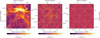 |
Fig. 1 Herschel SPIRE maps at 250 μm. Left: map of the Spider field, dS. Center: map of the LH field, dL. Right: data noise for the Spider observations, dN. |
2.2 LH region
LH is one of the fields targeted by the Herschel Multi-tiered Extragalactic Survey (HERMES, Oliver et al. 2012). Viero et al. (2013) have used the data to characterize the structure of the CIB with the power spectra. Their analysis shows that on this field the contamination of the extended emission by Galactic dust is much smaller than in the Spider field. We have used the Level 3 image.
The LH map at 250 μm was downloaded from the Herschel Database in Marseille (HeDaM4, Shirley et al. 2021), where the field is referred to as LOCKMAN-SWIRE. The image obtained after cropping the irregular edges and removing the ~40 galaxies whose peak brightness is over 6 MJy sr−1 is called dL and is presented in Fig. 1. The LH image is also a square with sides of 1144 pixels corresponding to 1.91 degrees on the sky. The pixel size is 6″ as for the Spider maps.
2.3 Power spectra
Figure 2 presents the power spectra of the dS, dL, and dN maps. The figure also includes the power spectrum of a SPIRE observation of Neptune at 250 μm. As in Miville-Deschênes et al. (2010), we consider Neptune as a point-like source and use this observation to compute the power spectrum of the point spread function (PSF).
The noise spectrum is flat for k > 0.2 arcmin−1. The flattening of the dS and dL spectra to different constant values at high k indicates that the noise power is one order of magnitude larger for the Spider observation. The dL spectrum shows the progressive attenuation of the sky emission by the telescope beam for k > 1 arcmin−1. This attenuation is not apparent for the dS map because the noise amplitude is higher.
We checked that the power spectrum for the LH field is consistent with the one presented by Viero et al. (2013). In Fig. 2, we also show the power spectrum of the dust emission in the LH field as estimated by Viero et al. (2013). We used their Eqs. (8) with P0 = 4.5 × 10⁵ Jy2 sr−1 and αc = −3.66. As the dust contribution is small except at the largest scale, the power spectrum of dL is essentially that of the CIB. The power spectrum of dS is dust dominated for k < 0.2 arcmin−1. The CIB contribution is significant for higher k.
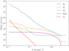 |
Fig. 2 Power spectra of Herschel SPIRE maps. The power spectra of the Spider map (dS) and data noise (dN) are compared to those of the LH field (dL) with the dust contribution, sL, as estimated by Viero et al. (2013). The spectrum of an observation of Neptune (dPSF), plotted with an arbitrary normalization, indicates the beam attenuation at high k. The wavenumber in abscissa is k = 1/θ. These spectra show that the CIB and noise components dominate the dust signal at the smallest scales in the dS map. |
3 Component separation method
In this section, we explain the procedure that allows us to derive a statistical model of the dust emission from the Spider Herschel observations. We present the mathematical formalism of the problem in Sect. 3.1 and our algorithm implementation in Sect. 3.2.
3.1 Mathematical formalism
We want to separate the dust emission from the CIB and the Herschel instrumental noise. This problem can be written as a system of three equations involving the three observational maps: dS, dL, and dN. The sky maps dS and dL include the dust, CIB, and noise, while the difference map dN is a noise map that is free from dust and from the CIB. We thus write:
 (2)
(2)
where s, c, and n terms represent the dust, CIB, and noise contributions to each image, respectively.
Our scientific objective is twofold. First, we aim to derive a statistical model of the dust emission from the Spider observation expressed in terms of WPH statistics. Second, we aim to derive an estimate of the Spider dust map sS as one specific realization of the dust model.
We simplify Eq. (2), neglecting sL with respect to cL and sS, and nL with respect to nS and cL. These simplifications are supported by the comparison of the dS, dL, and sL spectra in Fig. 2. In the following, we also consider that the CIB is a statistically isotropic signal on the celestial sphere, ignoring its correlation with the large-scale structure of the universe (Planck Collaboration XVIII 2014; Serra et al. 2014).
We rewrite Eq. (2) as:
 (3)
(3)
where we have introduced the map, c′L, which represents a hypothetical observation of LH with the data noise statistically matching that of the Spider observation. We also introduce c′S = cS + nS to rewrite Eq. (3) in terms of the WPH statistics:
 (4)
(4)
where Φ(m) are the WPH statistics (see Appendix B) computed for a map, m. The second equation follows from the isotropy of the CIB on the celestial sphere.
These equations lead us to consider two statistical processes: S associated with the dust emission and C′ associated with the sum of the CIB and the Spider data noise. Hereafter, we refer to S and C′ as the dust and contamination, respectively. The map sS is a realization of S, while the maps c′S and c′L are distinct realizations of C′. From the map, c′L, we can directly compute the WPH statistics that characterize C′. To characterize S we use a statistical component separation algorithm explained below.
3.2 Algorithm principle
The framework we used for statistical component separation has already been studied through the denoising of Planck interstellar dust polarization maps on a flat sky using WPH (Régaldo-Saint Blancard et al. 2021) and on the sphere, using an implementation of cross-WST on healpix (Delouis et al. 2022). We followed and extended the work of Régaldo-Saint Blancard et al. (2021). This method consists of an iterative minimization in pixel space of a loss function. We performed an iteration on a dust map, u, to converge to an estimator  of sS, such that the u + c′S map and the dS map become “close enough” in terms of WPH statistics.
The quantitative description of the algorithm is described by the loss function. The expression of our loss function ℒ(u) is:
 (5)
(5)
where
 (6)
(6)
where ||•|| stands for the Euclidean norm and 〈•〉i stands for the average over i and α is a real number that will be chosen to balance the two loss terms. The set {c′S,i}i<N represents N sky maps generated from the WPH statistics Φ(c′L) (see Appendix B.2). We use the WPH statistics defined as in Régaldo-Saint Blancard et al. (2022) and refer to Appendix B.1 for technical details. The WPH statistics used in this paper are made of 3441 coefficients. This definition includes a normalization which is done by using two reference maps, m1 and m2, one for each of the loss terms.
Our loss function, ℒ(u), is composed of two non-orthogonal terms. The ℒ1 term is the loss function used in Régaldo-Saint Blancard et al. (2021). It follows directly from the top line of Eq. (4). It constrains the u map such that if we add an independent realization of c′S, the sum has the same WPH statistics as dS. We averaged over several syntheses of c′S so that the separation does not depend on the deterministic properties of one specific realization of C′. The ℒ2 term follows from the bottom line of Eq. (4). It constrains the dS − u map, which we want to converge to c′S = dS − sS to have the same WPH statistics as c′S. In Régaldo-Saint Blancard et al. (2021), the contamination was a piece-wise Gaussian noise, while in our case, C′ is a non-Gaussian process. Experimentally, we found that the ℒ2(u) term is necessary to account for the non-Gaussianity of C′.
Recently, Régaldo-Saint Blancard et al. (2022) introduced cross-WPH statistics to capture the non-Gaussian correlations between different maps. They applied it successfully to the building of multifrequency dust generative models. Simultaneously, Delouis et al. (2022) developed cross-WST statistics on the sphere and applied it to the denoising of Planck interstellar dust polarization full-sky maps. The success of this method lies in the use of cross-statistics between half-missions maps with distinct data noises, and the TE dust correlation (Planck Collaboration Int. XXX 2016b), which makes use of the high signal-to-noise ratio (S/N) of the dust total intensity map. In our case, the same CIB sky signal is present in both half-missions maps, but we could have added a loss term based on the dust-H I correlation. We did not implement such a term because the H I data (Blagrave et al. 2017) has a lower angular resolution than the Herschel maps and a higher noise level.
To implement the algorithm, we need to choose α, the two reference maps, m1 and m2, used for the loss normalization and the initial value, u0, of the u map. These choices will be discussed in the following sections. At the end of the optimization, we converge to a map  . The WPH statistics of
  constitute the dust statistical model. The model may be used to generate new realizations where the optimal choice of the initial map depends on the scientific objective.
The maps generated from the statistical model have structure on all scales, including those where the power of the contamination is much larger than that of the dust. Our goal is to reproduce the non-Gaussian dust statistics even on the scales where we do not succeed in reproducing deterministically the true dust map (Régaldo-Saint Blancard et al. 2021; Delouis et al. 2022). Our approach differs from other attempts to separate the dust and CIB (Remazeilles et al. 2011) in two main ways: our component separation is based on non-Gaussian statistics and we do not seek to minimize the mean squared error in pixel space (see, e.g., Wiener 1949).
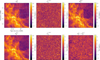 |
Fig. 3 Input and output maps for the component separation applied to the mock data. The three top images show the input dust map |


4 Validation on mock data
To validate our method, we applied our component separation algorithm to mock data. The mock data are introduced in Sect. 4.1. We compare input and output maps in Sect. 4.2. In Sect. 4.3, we show that the output maps reproduce statistics of the input mock data, which are used as diagnostics in interstellar astrophysics.
4.1 Mock data
We present how we built the mock data from observations to be as close as possible to the real data. We produce a set of mock maps defined as:
 (7)
(7)
where m stands for mock data and the i index indicates the different mock maps. Guided by the correlation between dust and gas in the high latitude sky (Lenz et al. 2019), we use an integrated intensity map, IH I of 21 cm data to build  as a pure dust map free from the CIB. Specifically, we made use of the DF dataset, located at (α, δ) = (10h30m,73°48′) (i.e., centred on the Spider field) that was part of the DHIGLS5 H I survey (Blagrave et al. 2017) with the Synthesis Telescope (ST) at the Dominion Radio Astrophysical Observatory. A detailed description of the DF dataset is presented in Appendix C, along with the procedure used to reduce noise in the data using the Gaussian decomposition algorithm ROHSA (Marchal et al. 2019). The velocity range of integration is −9.7 <υ< 26.5 km s−1. The IH I map is a square with 312 pixels on each side corresponding to 5.2 degrees on the sky. The sky region covered by the IH I map includes the one covered by the dS map.
To obtain  we scaled the IH I map, so that the power spectrum of
  would approximately match that of dS The
  map is used as a spatial template of clean dust emission at the Herschel resolution. The mock dust map is presented in the top left panel of Fig. 3. For the contamination, we use the c′L map that combines two Herschel maps: the LH CIB map, dL, and the noise map, dN of the Spider observation. Since the
  map has only 312 × 312 pixels, we cut the 1144 × 1144 contamination map, c′L, into nine independent patches of equal areas of 312 × 312 pixels. These patches allowed us to take into account the spatial variations of the CIB statistics over the LH region. They were combined into 72 independent pairs; for each pair, we used the first patch to produce the mock data and the second one as input to learn the statistics of the contamination. The mock
  were thus constructed as the sum of
  and
and  One pair of maps
  is plotted next to the
  map in Fig. 3.
We used the set to run our separation algorithm on these 72 different cases. The mean and the standard deviation of these results allow to verify that the algorithm does not produce a significant bias on the statistics of the dust map. Unfortunately, our validation is based on a small sample because the 72 cases are not independent. However, we are confident that this method, which allows us to take into account the non-Gaussianity of the CIB encoded in the observations, gives a satisfactory check of the significance of any potential bias. Using WPH syntheses (Appendix B.2), we could have generated more non-Gaussian realizations of the contamination to better sample the chance correlation with the dust mock map, but this possibility was constrained by the required computation time. It is important to take into account the variance of the CIB statistics to verify the algorithm ability to determine the dust statistics when there are small differences between the statistics of the patch,  , used to model the contamination, with respect to those of the contamination in
  This is only indicative because the variance between the contamination patches is not necessarily commensurate with the CIB variance on the sky between the LH and Spider fields.
4.2 Implementation of the component separation and results
Here, we describe the implementation of the component separation algorithm before presenting the output images. To apply the algorithm, we made the following choices for the initial map, u0, the maps used for the loss normalizations, m1 and m2, and the inter-loss weight, α (Sect. 3.2).
As in Régaldo-Saint Blancard et al. (2021), we chose  to obtain an output dust map reproducing the observed map on scales where the dust emission dominates. The m1 and m2 maps are used to normalize the WPH statistics versus scale in ℒ1 and ℒ2. The simplest normalization would be to use the mock observation
  for m1 and a contamination map
  for m2. Régaldo-Saint Blancard et al. (2021) showed that this choice for m1 is not optimal to reproduce the dust WPH statistics on the smallest scales, where the contamination is dominant. Ideally, we would need to know beforehand the dust power spectrum to give the appropriate weight to the dust WPH statistics. In practice, we ran the algorithm in two steps. First, with
  to converge to a first dust map,
  which does not reproduce the non-Gaussian statistics well, but has the proper dust power spectrum. For this first run, we only used the first loss term, ℒ1, computed on a subset of WPH statistics that only contain power spectrum-like terms.
Second, we ran the algorithm with the two loss terms with  and
and  . We choose α to give more weight to ℒ1 than to ℒ2 at the start of the gradient descent because we want the first loss to dominate at this point. This is because the second loss term is initially applied to an identically zero map, since uo = ds, and thus contains no information. We expect ℒ2 to help dS − и to converge to the statistics of the contamination in a second stage. We set α such that ℒ1 (u0) ~ 10α ℒ2(u0) and find that the result of the separation is only weakly dependent on this specific choice. For the validation algorithm, a run takes about 2 h on a 32 GB GPU.
The WPH statistics of  ,
,  ,
,  ,
,  , and
, and  are presented in Fig. D.1 and discussed in Appendix D. The figure shows that our specific choice of {u0, m1, m2, α} allows us to recover the WPH statistics of dust within error bars at all scales. This validates our algorithm with respect to our primary goal, which is to properly recover the non-Gaussian statistics of dust emission. Figure 3 presents the output maps of our separation algorithm applied on
  . Comparing by eye
  with
with  , we see that we have efficiently removed the contamination without losing the non-Gaussian structure of the dust emission down to the smallest scales. The comparison of
  and
and  is equally satisfactory. The standard deviation of
  ,
,  ,
,  ,
,  ,
,  , and
, and  are 2.39, 1.17, 2.61, 2.34, 1.17, and 0.64, respectively. The
  mock map does not exactly resemble the Herschel dS one because the first covers a much larger sky area than the second. The sky region covered by the dS map corresponds approximately to the quarter at the bottom left of
  .
.
In Fig. 4, we present the power spectra of the six maps shown in Fig. 3, plus the cross spectrum between  and
and  . These spectra have been computed on apodized maps and binned in order to lower the statistical variance at large values of k. Given the power spectra of
  and
and  are very close at all scales, the separation is able to recover the power spectrum of the dust map more than one order of magnitude under the contamination. The power spectra of
  and
and  are also very close, which could be expected since its directly constrained by the ℒ2 loss term. It shows the ability of our method to extract a realistic contamination from the components mixture.
The cross spectrum  shows the transition from a deterministic to a statistical separation at the scale of k = 0.7 arcmin−1, where the dust power becomes lower than that of the contamination. This transition is similar to that reported by Régaldo-Saint Blancard et al. (2021) and Delouis et al. (2022) for the denoising of Planck dust polarization maps. On the smallest scales,
  and
and  are two independent realizations of the dust statistics. This explains the factor of 2 difference between the power spectrum of
  and those of
  and
and  . Indeed, we see coherent features distributed at small scales in the difference map at the bottom right corner of Fig. 3, which testify to the displacement of structures from
  to
to  .
.
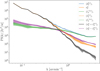 |
Fig. 4 Power spectra of the input and output maps of the component separation applied to the mock data. The figure shows the power spectra of |


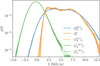 |
Fig. 5 PDFs of the dust intensity for the input and output maps of the component separation applied to the mock data. The PDFs of |


4.3 Non-Gaussian diagnostic for dust astrophysics
We show that the dust output maps reproduce statistics used as diagnostics to characterize the non-Gaussianity of interstellar imaging observations. We considered the probability distribution functions (PDFs) of the intensity and its spatial increments and the reduced wavelet scattering transform (RWST, Allys et al. 2019). The notation 〈•〉i represents the mean of the statistics computed over our set of 72 separations (Sect. 4.1), whereas the error bar is the standard deviation.
Figure 5 presents the PDFs of the dust intensity, which is commonly used as a diagnostic of the structure of molecular clouds (Burkhart 2021; Lombardi et al. 2015). The PDF of  is clearly biased towards low and high values by the contamination. After the component separation we recover very well, within statistical uncertainties, the PDF of the dust map
  . The PDF of the contamination map
  is also well recovered.
Figure 6 shows PDFs of the increments of the dust emission for three lags. The increment at a position x for a lag l in pixels is the set of differences δIl(x) = I(x) − I(x + l) with l <|l| < l + 1. Such PDFs have been computed on velocity maps (Hily-Blant et al. 2008) and polarization maps (Régaldo-Saint Blancard et al. 2021) to characterize the intermittence of turbulence in the ISM. The PDF of  is far more Gaussian than that of
  , especially for small pixel lags where the impact of the contamination is the largest. For the three lags, the PDF of
  matches the one of
  within statistical uncertainties over at least three orders of magnitude.
The RWST statistics are low-dimensional non-Gaussian interpretable statistics that has found many applications in astrophysics (Allys et al. 2019; Régaldo-Saint Blancard et al. 2020; Saydjari et al. 2021). They are briefly presented in Appendix E. We use here the  ,
,  ,
,  , and
, and  coefficients. Figure 7 presents those RWST statistics for
  ,
,  and
and  . The
. The  and
and  characterize the amplitude as well as the level of anisotropy as a function of scales, respectively. The
  characterize the couplings between different scales, while the
  describe their isotropic angular modulation (Allys et al. 2019). The RWST statistics of
  are strongly biased by the contamination. We can also notice that the RWST statistics of
  and
and  are very close with respect to that of
  at most of the scales, but we can notice small discrepancies at the smallest scales.
In the three examples presented in Figs. 5–7 we see that these non-Gaussian statistics of  are very well recovered through our component separation method. This result illustrates the possibility of using the WPH model to determine non-Gaussian statistics that are not directly constrained in the component separation. It demonstrates the relevance of the WPH statistics for astrophysics. We point out the large difference between the statistics of
  and those of
  , which shows that the component separation step is essential to build a precise non-Gaussian statistical model of the dust emission.
5 Application to Herschel SPIRE observations
We applied our component separation method to the Herschel observation of the Spider field, dS (Sect. 5.1). The power spectrum of the output map is presented and analyzed in Sect. 5.2. In Sect. 5.3, we present images that highlight a main non-Gaussian feature of the dust maps: the correlation between structures across scales.
5.1 Herschel separation results
Our algorithm is applied to the dS map as described in Sect. 4.2. We increased the pixel size of the image from 6″ to 12″ because the dust emission is highly attenuated by the beam on those scales (more than five orders of magnitude at 6″). This resampling is done using a low-pass filter in Fourier space with kmax = 2.5 arcmin−1 equal to the Nyquist frequency for 12″ pixels. This filtering does not induce ringing in the map because the beam attenuation on the signal power at k = 2.5 arcmin−1 is large (about a factor 65). Furthermore, for the purposes of normalization, it allows us to keep the exact same procedure from the validation on mock data to this case.
The component separation algorithm was applied according to the steps given in Sect. 4.2 for the mock data. We choose u0 = dS for the initial map. First, we run the algorithm using only the ℒ1 loss term, computed on a subset of WPH statistics that only contain power spectrum-like terms, with m1 = dS to produce an intermediate dust map  . Second, we run the algorithm using the two loss terms with
  and m2 = c′L We set α such that ℒ1(u0) ~ 10α ℒ2(u0). In this case, a run of the algorithm takes about 8 h on a 32 GB GPU.
In Fig. 8, we present the output maps of our separation algorithm applied on the Spider Herschel observation. From a visual point of view, the results are very satisfactory: it indeed seems that most of the CIB contamination has been identified as such. It is notably the case of all galaxies that are individually resolved, which is not surprising because they have an extremely clear non-Gaussian signature, both in terms of frequency and spatial location. Conversely, it does not seem that structures related to Galactic dust have leaked to the reconstructed contamination above the scales where it begins to dominate. This is impressive for results that have been obtained from three observational patches only. It should be noted, however, that the CIB reconstruction has visual defects at the position of the very bright horizontal Galactic dust structure at the top of the image. We believe that this is due to the limitation of considering the dust emission as a statistically homogeneous signal6.
The WPH statistics of the output and input Spider maps  and dS are discussed in Appendix D and compared in Fig. D.2. The WPH statistics of
  constitute our statistical model of the dust emission. Figure D.2 also presents the statistics of c′L and
  . The main scientific results of the component separation algorithm are the statistics of the dust emission and, in particular, its WPH statistics. They are obtained from the
  map, which is a realization of the estimated WPH statistical model of the dust emission, conditioned by its large scales, where the dust power is dominant. The
  map is then highly correlated at large scales with the dS map, up to a scale where there is a transition from a deterministic to a statistical behavior (Régaldo-Saint Blancard et al. 2021; Delouis et al. 2022).
From the WPH statistical model, we can generate diverse dust maps depending on the specific choice of the initial map, u0, and the scientific goal. For example, we can use an H I map as initial condition to ensure that it is decorrelated from the CIB. For other statistical applications, it is useful to have multiple realizations of the dust emission. In terms of this ability to generate various dust maps, our method differs from deterministic component separations.
Once we ran the component separation algorithm on the Herschel observation, we obtained a dust map that provides us with an estimate of the non-Gaussian statistics of the dust emission, which are not biased by the CIB and noise. We then estimated the error bars on these dust statistics as follows. We did not use the error bars determined on the mock data because the statistics of the mock dust map only approximate the true statistics of the dust emission, in particular, because it is based on an H I observation with a lower resolution than the one of the Herschel observations. First, we used the WPH synthesis method (described in Appendix B.2) to synthesize ten new realizations of the dust from our separated dust map,  , and ten new realizations of the contamination from the contamination map c′L. Summing these new dust and contamination maps, we obtain ten mock mixture maps, to which we apply the component separation algorithm to obtain ten new separated dust maps. The standard deviations of the statistics computed over these ten dust maps are then taken as error bars. We note that in this procedure, we cannot use patches of the LH and noise maps to define different contamination samples because the Spider image is as large as them. Unfortunately, this does not allow us to take into account the spatial variations of the contamination statistics in our estimate of the error bars.
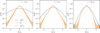 |
Fig. 6 PDFs of increments of the dust intensity for the input and output maps of the component separation applied to the mock data. The PDFs of |


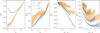 |
Fig. 7 RWST statistics of the input and output maps of the component separation applied to the mock data. The RWST statistics of |


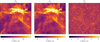 |
Fig. 8 Input and output maps for the component separation applied to Herschel SPIRE maps at 250 μm. Left: map of the Spider field dS. Center: output dust map |


5.2 Power spectra
Figure 9 presents the beam-corrected power spectrum of dS, the beam-corrected power spectrum of  , and its power-law fit. These spectra have been computed on apodized maps and binned in order to lower the statistical variance at large k. At k = 2 arcmin−1, the power of
  is two orders of magnitude lower than that of dS.
Figure 9 shows that the power spectrum of  is very close to a power-law after beam correction. To estimate the spectral index of the power-law and its uncertainty, we need to add to the component separation uncertainty the cosmic variance. We must do this because we characterize a statistical process using an observation (one realization of the process) of finite sky area A. The standard deviation of the dust power spectrum computed at wavenumber k is:
 (8)
(8)
where Nk is the number of modes at wavenumber k. This leads to
 (9)
(9)
where the wavenumber k and the bin size ∆k are expressed in rad−1 (Scott et al. 1994; Knox 1995). We compute the total uncertainty as the quadratic sum of σk and the component separation uncertainty and perform a power-law fit of the beam-corrected power spectrum of  in log scale. The bottom panel of Fig. 9 presents the beam-corrected power spectra of dS and
  divided by the power-law fit7. We can see that the power-law fits well the beam-corrected power spectrum of
  until k = 2 arcmin−1. This result is satisfactory because it indicates that the component separation algorithm did not filter out the small scales up to a k value, where the power of
  is about 2% of that of dS. The maximum wavenumber up to which the power-law shape is measured is thus increased by almost a decade by the component separation.
The slope of the spectrum is −2.95 ± 0.04. We compare this fit result with values measured for the Polaris Flare, a brighter field observed by Herschel (Miville-Deschênes et al. 2010), as well as for a diffuse cloud using Planck, WISE and optical data (Miville-Deschênes et al. 2016). In both cases, the CIB is subdominant and is neglected. The power spectrum of the dust maps is a power-law in both fields, but the slope in log scale goes from −2.65 in Polaris to −2.9 ± 0.1 for the diffuse cloud. The slope we find is consistent with the latter value.
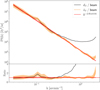 |
Fig. 9 Power spectra of the input and output maps for the component separation applied to Herschel SPIRE maps at 250 μm. Top: beam-corrected power spectrum of dS, beam-corrected power spectrum of |

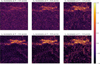 |
Fig. 10 Maps of increments for the component separation applied to Herschel Spider observations. The Neperian logarithm of the absolute value of the increments computed at θ = 0.4, 0.8, and 1.6 arcmin lags are compared for the input (dS, top row) and output ( |

5.3 Coherent structures
The component separation allows us to identify coherent structures that are hidden by the CIB in the SPIRE maps. To illustrate this result, we computed the maps with increments for different lags, presented in this work. Computed on a map I at a lag l, the pixel at the position x of the increment map is the mean of {I(x) − I(x′), |x−x′| = l}. In the following, the dust statistics are computed at 0.4, 0.8, and 1.6 arcmin. These scales corresponds to wavenumbers 2.5, 1.25, and 0.625 arcmin−1.
Figure 10 shows the increment maps of dS and  . One can identify coherent structures on both sets of increments maps, with a much improved contrast for
  . The component separation also highlights the correlation between coherent structures at different scales. This result extends earlier results obtained with wavelet convolution of IRAS sky maps (Abergel et al. 1996; Jewell 2001; Miville-Deschênes et al. 2007) and with Herschel observations on brighter clouds (Robitaille et al. 2019) to smaller angular scales.
6 Non-Gaussian statistics of the diffuse dust emission
Here, we quantify the non-Gaussian statistics of diffuse dust emission in the Spider field and compare our results with earlier studies.
6.1 Coherent structures across scales
The RWST statistics (see Appendix E) provide statistical insights into the multiscale filamentary structure of the cold neutral medium. The dust and CIB separation allows us to expand on the analysis of Herschel and H I data presented by Allys et al. (2019) and Lei & Clark (2023).
Figure 11 presents two RWST coefficients that characterize correlations between scales (Allys et al. 2019). Both are plotted versus the scale ratio (j2 − j1). In each plot, the  statistics are compared to those of the map
  obtained by randomizing the phase of the Fourier transform of
  . This comparison highlights deviations from Gaussianity. Unlike the Gaussian field, the
  of
of  do not depend solely on j2 – j1. This result shows that the dust emission is not statistically scale-invariant. The
  coefficients quantify the angular modulation of the coupling between scales. The angle dependence relates to the filamentary structure of the diffuse ISM because it measures how the coupling between two scales varies between the aligned and orthogonal orientations. The non-vanishing values of
  of
of  at large j2 – j1 testify of the presence of long filaments.
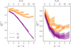 |
Fig. 11 RWST statistics of the output dust map for the component separation applied to Herschel SPIRE maps at 250 μm. The |


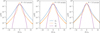 |
Fig. 12 Increment PDFs of the input and output dust maps for the component separation applied to Herschel SPIRE maps at 250 µm. The increment δI of ds, |


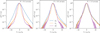 |
Fig. 13 Wavelet coefficents of the input and output dust maps for the component separation applied on the Herschel Spider map. The PDFs of the real part of the wavelet coefficients of dS, |


6.2 Signatures of turbulence intermittency
Statistics of velocity increments derived from CO observations results have been theoretically interpreted as a signature of intermittency of interstellar turbulence (Falgarone et al. 2015). The same result is theoretically expected for the dust polarization and the gas column density (Momferratos 2015).
Figure 12 presents the PDFs of the increment images of  shown in Fig. 10. The PDFs are roughly scale-invariant. They display non-Gaussian wings with no clear trend with the lag. This result contrasts with what has been reported for other observables. Indeed, the PDFs of increments computed for the gas velocity from spectroscopic CO observations (Hily-Blant et al. 2008) and for the dust polarization from Planck data (Régaldo-Saint Blancard et al. 2021) show non-Gaussian wings that become increasingly prominent for decreasing lag.
6.3 Structure formation in the diffuse ISM
The formation of structure in the cold interstellar medium is thought to be driven by the interplay between the turbulent gas dynamics and thermal instability (Kritsuk & Norman 2002; Saury et al. 2014). The statistics of dust maps provide observational insight. Miville-Deschênes et al. (2007) presented PDFs of wavelet convolutions of IRAS dust images. They have on all scales a pronounced skewness, which they relate to the non-linearity of the dynamical processes driving the formation of structures. The Herschel data and the dust and CIB separation allow us to extend this analysis to smaller angular scales.
Figure 13 shows PDFs of wavelet convolutions on angular scales from 0.4′ to 1.6′, well below the IRAS 5′ resolution. The wavelets are those used for the WPH data analysis. The PDFs of  exhibits non-Gaussian wings, but smaller skewness than that of dS. Table 1 contains the skewness and kurtosis of wavelet convolutions at scales from 0.4′ to 12.8′. These values describe the shape of the PDFs. Our values are not directly comparable to those computed by Miville-Deschênes et al. (2007) on IRAS maps because we use directional wavelets instead of isotropic wavelets.
Skewness and kurtosis of the wavelet convolutions of the dust map at 0.4′, 0.8′, 1.6′, 3.2′, 6.4′, and 12.8′.
7 Conclusion
We have made use of the distinct textures of the CIB and the dust emission on the sky to develop and apply a component separation method on Herschel observations at a single frequency. The main results of our work are as follows.
The component separation problem on Herschel data involve three components: the dust, the CIB, and the data noise. We reduce this problem to a single inverse problem in terms of WPH statistics and present an algorithm to solve it. The results of this algorithm are a WPH generative model of the dust emission and an output map which is a realization of the model correlated with the input map.
We build a set of realistic mock data using an H I map as a template of CIB-free dust emission map. These data are used to validate the method. We show that we are able to retrieve the WPH statistics of the dust emission as well as non-Gaussian statistics used in astrophysics to characterize interstellar imaging data. Unlike methods that minimize the mean squared error in pixel space, we reproduce the power spectrum of the input map down to the smallest angular scales.
The method is applied to a Herschel SPIRE observation of diffuse interstellar matter at 250 µm. We succeed in performing a statistical separation from observational data only at a single frequency by using non-Gaussian statistics. The power spectrum of the output map is well fitted by a power-law up to k = 2 arcmin−1, where the dust signal represents 2% of the total power. The obtained slope is −2.95 ± 0.04.
We analyzed the non-Gaussian properties of the Spider dust emission on scales where the CIB signal is dominant. The component separation step is essential for characterizing the non-Gaussianity of the dust emission. Going beyond a standard power spectra analysis, we show that the non-Gaussian properties of the dust emission are not scale-invariant. The separated dust map reveals coherent structures at the smallest scales. This work offers several perspectives for future work:
We underline that we use in this paper only one of the three wavelengths of Herschel SPIRE. Thanks to the recent development of cross-WPH statistics (Régaldo-Saint Blancard et al. 2022), our method could be extended to a multi-channel component separation of the dust and CIB on Herschel data with an aim to statistically characterize the dust SED;
We could use external templates as an H I observation for the dust;
It would also be useful to compare the gas and dust to test whether these two interstellar components are coupled on small angular scales for the cold and warm phases. This work could also be extended to other fields mapped with SPIRE;
Our statistical component separation could also be used on Planck data to separate the dust and CIB up to larger angular scales on the sphere.
Acknowledgements
We thank F. Levrier and J.-M. Delouis, as well as S. Mal-lat and R. Morel for helpful discussions. We also thank the anonymous referee for valuable comments that helped to improve the paper. Software: PyWPH (Régaldo-Saint Blancard et al. 2021), PyWST (Régaldo-Saint Blancard et al. 2020).
Appendix A Mathematical notations
Summary of the main mathematical notations.
Appendix B WPH statistics
We present our construction of the WPH statistics and explain how it can be used as a generative model. This brief overview is directly inspired by Régaldo-Saint Blancard et al. (2021).
Appendix B.1 Definition
The construction of the WPH statistics follows two main steps: i) a multi-scale decomposition of the process under study into its different components and ii) the characterization of the interaction between its different scales.
The first step consists of performing a multi-scale decomposition using a wavelet transform. The wavelets we use are bump steerable wavelets (Zhang & Mallat 2019). These wavelets ψj,l(x) are indexed by two integers, j ∈ [0, J – 1] and l ∈ [0, L – 1], which define the oriented scale they characterize: ψj,l(x) is the wavelet used to probe the 2j characteristic scale at an angle  from the reference axis. The wavelet transform of a process ρ(x) is defined as the set of its convolutions ρ * ψj,l(x) with wavelets at all oriented scales. It performs a multi-scale decomposition of ρ, decomposing its structures on the different scales probed by the wavelets: indeed, by convolving an image with a wavelet, we make a local filtering on the wavelet band-pass. This decomposition is illustrated in Fig. B.1, which shows the modulus and phase of convolutions of the dS map with several wavelets. For a given wavelet ψj,l, the modulus of the convolution dS * ψj,l highlights the structures of dS for a scale of 2j and orientation of
  .
.
The second step of this transform is to characterise the interaction between the different scales of the process, ρ, under study. A natural way to characterize such an interaction is to compute the covariances between the different ρ * ψj,l(x) terms of the wavelet transform. However, such covariances are not able to characterize non-Gaussian features. Indeed, we can show (see, e.g., Allys et al. (2020)) that:
 (B.1)
(B.1)
where S (k) is the power spectrum of ρ, which only characterize each wavenumber, k, independently. This shows that in order to characterize coupling between scales, it is necessary to introduce non-linearities.
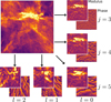 |
Fig. B.1 Modulus and phase of the convolutions of dS with ψ3,0, ψ4,0, ψ5,0, ψ5,1, and ψ5,2. In this example, we set L = 4. |
The second step to construct WPH statistics thus consists in introducing non-linearities in order to characterize interactions between scales. Indeed, if we want to get an information from the covariance between two fields, they must have common frequencies. We can take the modulus of the different wavelet convolutions, but also use a non-linear operator to capture information about phase alignement between different scales. This operator is the Phase Harmonics operator, which is defined as:
![Mathematical equation: $ \forall z \in ,\forall p \in ,\quad {[z]^p} = |z|{e^{i\,\,\arg \left( z \right)\, \times p}}. $](/articles/aa/full_html/2024/01/aa46814-23/aa46814-23-eq181.png) (B.2)
(B.2)
For p ≠ 0, this operator multiplies the complex phase of a field by a constant integer, computing the harmonics of its phase. This operator makes the phase of the two filtered images vary at the same spatial frequency in order to characterize the statistical phase alignment by means of a covariance.
We can now construct different “WPH moments,” by computing covariance of phase harmonics of wavelet convolutions which share common frequencies, namely, whose spectral supports overlap. The WPH moments depend on a translation vector, τ, that allows us to increase the spectral resolution. The general expression of WPH moments is:
![Mathematical equation: $ \forall z \in ,\forall p \in ,\quad {[z]^p} = \left| z \right|{e^{i\,\,\arg \left( z \right)\, \times p}}. $](/articles/aa/full_html/2024/01/aa46814-23/aa46814-23-eq182.png) (B.3)
(B.3)
The number of translation vectors considered is 1 + 8Δn. We note that due to the choice of the harmonics p1 and p2, there are different ways to couple a pair of scale.
The summary statistics we will use are WPH statistics, which are built from a set of WPH moments. In this work, we take a set of moments defined in Régaldo-Saint Blancard et al. (2022). This is a small modification of Allys et al. (2020), in which the set of moments has been chosen to construct a generative model of the large-scale structure matter density field (Allys et al. 2020). With J = 7, L = 4, and Δn = 2, it gives a set of 3441 moments. To describe these moments, we will follow the notations of this paper and define several types of moments: if the two scales are equal, we use the letter S, and if not, we use a C; the type of moment is identified by their respective harmonics p1 and p2.
The harmonics, p, multiply the frequency of a signal by a factor, p. As we want similar frequencies in order to have meaningful moments, several choices of harmonics are possible for a given pair of scales. First, we can take (p1, p2) = (0,0), which will lead to common frequencies even if the scales are different. We can also take (p1, p2) = (0,1) which will lead to common frequencies if j2 > j1. Finally, if we want to keep the phases and to take different scales, we have to choose p1 and p2 such that j1 p1 ~ j2p2, and the simplest choice is then to take (p1, p2) = (1,  ). For j1 = j2, it boils down to (p1, p2) = (1,1) which leads to the power spectrum-like moments, which we refer to the S11 moments (see Eq. B.1). For each type of moments, the particular moment is then labelled by the characteristic spatial frequencies probed (one for S term, two for C terms), indexed by their couple (j, l). For example,
  is the moment whose expression is
  .
.
We will use six types of moments: S11, S00, S01, Cphase, C00, and C01, whose expressions are as follows:
![Mathematical equation: $ \matrix{ {S_{j,l}^{11}\left( {\bf{\tau }} \right) = {\rm{Cov}}\left( {\left( {\rho * {\psi _{j,l}}} \right)\left( {\bf{x}} \right),\left( {\rho * {\psi _{j,l}}} \right)\left( {{\bf{x}} + {\bf{\tau }}} \right)} \right),} \hfill \cr {S_{j,l}^{00}\left( {\bf{\tau }} \right) = {\rm{Cov}}\left( {\left| {\rho * {\psi _{j,l}}} \right|\left( {\bf{x}} \right),\left| {\rho * {\psi _{j,l}}} \right|\left( {{\bf{x}} + {\bf{\tau }}} \right)} \right),} \hfill \cr {S_{j,l}^{01}\left( {\bf{\tau }} \right) = {\rm{Cov}}\left( {\left| {\rho * {\psi _{j,l}}} \right|\left( {\bf{x}} \right),\left( {\rho * {\psi _{j,l}}} \right)\left( {{\bf{x}} + {\bf{\tau }}} \right)} \right),} \hfill \cr {C_{{j_1},{l_1},{j_2},{l_2}}^{{\rm{phase}}}\left( {\bf{\tau }} \right) = {\rm{Cov}}\left( {\left( {\rho * {\psi _{{j_1},{l_1}}}} \right)\left( x \right),{{\left[ {\rho * {\psi _{{j_2},{l_2}}}} \right]}^{{{{j_1}} \mathord{\left/ {\vphantom {{{j_1}} {{j_2}}}} \right. \kern-\nulldelimiterspace} {{j_2}}}}}\left( {{\bf{x}} + {\bf{\tau }}} \right)} \right),} \hfill \cr {C_{{j_1},{l_1},{j_2},{l_2}}^{00}\left( {\bf{\tau }} \right) = {\rm{Cov}}\left( {\left| {\rho * {\psi _{{j_1},{l_1}}}} \right|\left( x \right),\left| {\rho * {\psi _{{j_2},{l_2}}}} \right|\left( {{\bf{x}} + {\bf{\tau }}} \right)} \right),} \hfill \cr {C_{{j_1},{l_1},{j_2},{l_2}}^{01}\left( {\bf{\tau }} \right) = {\rm{Cov}}\left( {\left| {\rho * {\psi _{{j_1},{l_1}}}} \right|\left( x \right),\left( {\rho * {\psi _{{j_2},{l_2}}}} \right)\left( {{\bf{x}} + {\bf{\tau }}} \right)} \right).} \hfill \cr } $](/articles/aa/full_html/2024/01/aa46814-23/aa46814-23-eq186.png) (B.4)
(B.4)
All these moments depend on the amplitude of the image power spectrum, but we want to have coefficients describing the non-Gaussian features only. Using Eq. B.1, we can show that the power spectrum information is contained in the S11 moments. Then, by normalizing all the moments by the S11 and the S00 ones, we get coefficients that describe non-Gaussianity independently of the power spectrum. For example, the expressions of the normalized C01 moments are  .
.
Appendix B.2 WPH generative model
Generative models can be constructed from the WPH statistics of a given process. Here, this was done within the framework of maximum entropy models, in a microcanonical approach, which boils down to constructing the most general probability distribution under the WPH constraints (Bruna & Mallat 2019). For a given statistical process, X, the WPH statistics allow to obtain new realizations, Xi, from a distribution estimated on an observation, X0. Starting from a white noise, we perform a gradient descent in pixel space in order to reproduce the WPH statistics of X0. Hereafter, we call this process a synthesis.
Many physical processes having power spectrum that vary over several orders of magnitude, their WPH statistics have very different values from one scale to another. This is a problem for the gradient descent because it gives an important weight to some scales, whereas others could be very little constrained. To prevent this problem, we normalize the WPH operator such that each WPH coefficient, which characterizes the coupling between two scales, is divided by the square root of the product of the power spectra of X0 at the corresponding scales. The reference map, m (defined in Sect. 3.2) is then set in this case to X0.
On a practical level, a synthesis is done using a gradient descent on a map u (where u0 is a white noise) to minimize the loss Lsyn(u) = ||Φ(u) – Φ(X0)||2, where Φ is the WPH operator. The result of the optimization is a new realization of the unkown process X estimated on X0, fully independent of X0. Allys et al. (2020) showed that the WPH generative model reproduces usual non-Gaussian statistics in cosmology up to 1-10%. The ability to build a non-Gaussian generative model is necessary for our component separation algorithm.
Appendix C H I map
The angular resolution of the ST interferometric data used as a spatial template of Galactic emission uncontaminated by the CIB is 0.91′ and the pixel size is 18″. The DHIGLS DF product has the full range of spatial frequencies, obtained by a rigorous combination of the ST interferometric and GBT single dish data (see Section 5 in Blagrave et al. 2017). At small scales, IH I is highly affected by noise, resulting in an increase of power at high k (Blagrave et al. 2017, see their Fig. 22). The statistical properties of this noise is complex and can potentially alter the quality of the separation performed as a validation test. Because IH I is only used as a template to generate a CIB-free SPIRE mock observation, we performed a denoising of the H I data cube prior integration along the velocity axis (from −9.7 to 26.5 km/s) to obtain a map of IH I in the Spider region with reduced data noise.
This was accomplished using the ROHSA algorithm (Mar-chal et al. 2019). While earlier applications were dedicated to phase separation (e.g., Marchal et al. 2021; Marchal & Miville-Deschênes 2021; Taank et al. 2022), here we make use of the spatial regularization of ROHSA to obtain a spatially coherent model of the data, which concurrently reduces noise. We first experimented with the decomposition of the DF dataset presented in Marchal & Martin (2023) that provides a full encoding of the data with N = 6 Gaussians and the hyper-parameters λa = λµ = λσ = λσ′ = 10, which control the strength of the regularization. Upon inspecting the resulting model, we found that the spatially correlated noise still dominates the signal on small scales in the IH I map. To overcome this limitation, we performed a new decomposition using higher hyper-parameters λa = λµ = λσ = λσ′ = 1000 to control the spatial regularization and intentionally reduce the noise even further. The resulting model does not encode the signal fully (due to the strong regularization), which translates into a chi-square map that is not as uniform as the original decomposition. We emphasize that the goal of this procedure is solely to generate a realistic mock observation of Galactic dust based on existing high-resolution H I data of the Spider, but IH I is not a component of our wavelet-phase harmonic-based method.
Appendix D WPH statistics of the separation results on mock and Herschel data
Here, we explain how to read the WPH statistics plots and we present the WPH statistics of the component separation results both on mock data (Fig. D.1) and on Herschel observations (Fig. D.2). These figures present the WPH statistics computed with Δn = 0 (no translation). Fhe values of S11, S00, and S01, which characterize a dyadic scale and an angle, are averaged over the angles and plotted as a function of the scale, j1, that they characterize. Fhe Cphase values, characterized by two scales and an angle, are averaged over the angles and plotted in lexicographic order as a function of j1 and j2. The C00 and C01 values, which are characterized by two scales and two angles, are averaged over the two angles at constant difference and plotted in lexicographic order as a function of j1 ∈ [0, J – 1], j2 ∈ [j1 + 1, J – 1] and Δl ∈ [0, L – 1] as the angle difference.
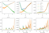 |
Fig. D.1 WPH statistics of the input and output maps for the component separation applied on the mock data. The WPH statistics of |


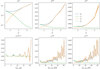 |
Fig. D.2 Same as Fig. D.1 but for the Herschel SPIRE maps at 250 µm. The WPH statistics of dS, |


Appendix E (R)WST statistics
The reduced wavelet scattering transform (RWST) statistics are interpretable non-Gaussian statistics defined in Allys et al. (2019). They are a reduced form of the wavelet scattering transform (WSF) statistics, first introduced in the field of data science (Mallat 2012). This brief overview is directly inspired by Allys et al. (2019).
Appendix E.1 WST statistics
The WST statistics are statistical descriptors that give a non-Gaussian description of a field. This is done by quantifying the level of coupling between scales. The WST are built by successive convolutions of the field with band-pass wavelets followed by the application of the modulus operator. Each of these summary statistics is then labeled by the scales they characterize.
We consider a two-dimensional field named ρ(x). As for the WPH statistics, the set of computed coefficients depends on two integers J and Θ, characterizing, respectively, the number of dyadic scales and angles considered. The integer scales j are labelled from 0 to J – 1 and correspond to 2j pixel scales, whereas the angles ϑ are labelled by integers θ ∈ [1,Θ], such that ϑ = (θ – 1)π/Θ. The set of wavelets is then {ψj,θ(x), j ∈ [0, J – 1], θ∈ [1,Θ]}.
The WST coefficients are computed in three layers labelled by the integer m going from 0 to 2. The only coefficient of the m = 0 layer characterizes the average of the field:
 (E.1)
(E.1)
where µ0 is the surface of integration. The coefficients S1 (j1, θ1) of the m = 1 layer depend on a single oriented scale (j1, θ1) and are defined as:
 (E.2)
(E.2)
where µ1 is the impulse response
 (E.3)
(E.3)
with δ the Dirac delta function. Finally, the coefficients S2(j1, θ1, j2, θ2) of the m = 2 layer depend on two oriented scales (j1, θ1) and (j2, θ2), and are defined as:
 (E.4)
(E.4)
where µ2 is defined in the same way as µ1. These coefficients are then normalized to separate the dependencies of the different layers. To this end, the coefficients of each layer are normalized by those of the previous layer. The normalized coefficients are denoted  and defined as:
 (E.5)
(E.5)
and
 (E.6)
(E.6)
whereas  . These coefficients provide a rich non-Gaussian statistical description of non-Gaussian fields.
Appendix E.2 RWST statistics
The regularity of certain physical fields leads to possible simplifications of the WST statistics. The RWST allows for the information contained in the WST to be concentrated into fewer coefficients, that are also more interpretable. This is done by fitting the angular dependencies of the logarithm of the WST coefficients with terms describing low-harmonics angular modulations.
The only angular dependency of the m = 1 layer coefficients is on θ1. The log2 [S1] coefficients are then written as:
![Mathematical equation: $ \matrix{ {{{\log }_2}\left[ {{{\bar S}_1}\left( {{j_1},{l_1}} \right)} \right] = \hat S_1^{{\rm{iso}}}\left( {{j_1}} \right) + } \hfill \cr {\quad \quad \quad \hat S_1^{{\rm{aniso}}}\left( {{j_1}} \right) \times \cos \left( {{{2\pi } \over {\rm{\Theta }}}\left[ {{\theta _1} - {\theta ^{{\rm{ref}},1}}\left( {{j_1}} \right)} \right]} \right),} \hfill \cr } $](/articles/aa/full_html/2024/01/aa46814-23/aa46814-23-eq203.png) (E.7)
(E.7)
where θref,1(j1)is a reference angle describing the global anisotropy direction of the field. The m = 2 layer is written using four terms and another reference angle:
![Mathematical equation: $ \matrix{ {{{\log }_2}\left[ {{{\bar S}_2}\left( {{j_1},{\theta _1},{j_2},{\theta _2}} \right)} \right] = \hat S_2^{{\rm{iso}},1}\left( {{j_1},{j_2}} \right)} \hfill \cr {\quad \quad + \hat S_2^{{\rm{iso}},2}\left( {{j_1},{j_2}} \right) \times \cos \left( {{{2\pi } \over {\rm{\Theta }}}\left[ {{\theta _1} - {\theta _2}} \right]} \right)} \hfill \cr {\quad \quad + \hat S_2^{{\rm{aniso}},1}\left( {{j_1},{j_2}} \right) \times \cos \left( {{{2\pi } \over {\rm{\Theta }}}\left[ {{\theta _1} - {\theta ^{{\rm{ref}},2}}\left( {{j_1},{j_2}} \right)} \right]} \right)} \hfill \cr {\quad \quad + \hat S_2^{{\rm{aniso}},2}\left( {{j_1},{j_2}} \right) \times \cos \left( {{{2\pi } \over {\rm{\Theta }}}\left[ {{\theta _2} - {\theta ^{{\rm{ref}},2}}\left( {{j_1},{j_2}} \right)} \right]} \right).} \hfill \cr} $](/articles/aa/full_html/2024/01/aa46814-23/aa46814-23-eq204.png) (E.8)
(E.8)
We refer to Allys et al. (2019) for an additional discussion on the interpretation of these coefficients.
References
- Abergel, A., Boulanger, F., Delouis, J. M., Dudziak, G., & Steindling, S. 1996, A&A, 309, 245 [NASA ADS] [Google Scholar]
- Allys, E., Levrier, F., Zhang, S., et al. 2019, A&A, 629, A115 [NASA ADS] [CrossRef] [EDP Sciences] [Google Scholar]
- Allys, E., Marchand, T., Cardoso, J. F., et al. 2020, Phys. Rev. D., 102, 103506 [NASA ADS] [CrossRef] [Google Scholar]
- André, P., Men’shchikov, A., Bontemps, S., et al. 2010, A&A, 518, A102 [Google Scholar]
- Béthermin, M., Wang, L., Doré, O., et al. 2013, A&A, 557, A66 [NASA ADS] [CrossRef] [EDP Sciences] [Google Scholar]
- Blagrave, K., Martin, P. G., Joncas, G., et al. 2017, ApJ, 834, 126 [Google Scholar]
- Boulanger, F., Abergel, A., Bernard, J. P., et al. 1996, A&A, 312, 256 [Google Scholar]
- Bruna, J., & Mallat, S. 2013, IEEE Trans. Pattern Anal. Mach. Intell., 35, 1872 [CrossRef] [Google Scholar]
- Bruna, J., & Mallat, S. 2019, Math. Stat. Learn., 1, 257 [CrossRef] [Google Scholar]
- Burkhart, B. 2021, PASP, 133, 102001 [NASA ADS] [CrossRef] [Google Scholar]
- Cheng, S., & Ménard, B. 2021, arXiv e-prints [arXiv:2112.01288] [Google Scholar]
- Chiang, Y.-K., & Ménard, B. 2019, ApJ, 870, 120 [Google Scholar]
- Delouis, J. M., Allys, E., Gauvrit, E., & Boulanger, F. 2022, A&A, 668, A122 [NASA ADS] [CrossRef] [EDP Sciences] [Google Scholar]
- Falgarone, E., Momferratos, G., & Lesaffre, P. 2015, in Astrophys. Space Sci. Lib., 407, Magnetic Fields in Diffuse Media, eds. A. Lazarian, E. M. de Gouveia Dal Pino, & C. Melioli, 227 [NASA ADS] [CrossRef] [Google Scholar]
- Gautier, T. N. I., Boulanger, F., Perault, M., & Puget, J. L. 1992, AJ, 103, 1313 [NASA ADS] [CrossRef] [Google Scholar]
- Griffin, M. J., Abergel, A., Abreu, A., et al. 2010, A&A, 518, A3 [Google Scholar]
- Hauser, M. G., & Dwek, E. 2001, ARA&A, 39, 249 [Google Scholar]
- Heiles, C. 1984, ApJS, 55, 585 [NASA ADS] [CrossRef] [Google Scholar]
- Heiles, C. 1989, ApJ, 336, 808 [NASA ADS] [CrossRef] [Google Scholar]
- Hennebelle, P., & Inutsuka, S. I. 2019, Front. Astron. Space Sci., 6, 5 [NASA ADS] [CrossRef] [Google Scholar]
- Hily-Blant, P., Falgarone, E., & Pety, J. 2008, A&A, 481, 367 [NASA ADS] [CrossRef] [EDP Sciences] [Google Scholar]
- Jewell, J. 2001, ApJ, 557, 700 [NASA ADS] [CrossRef] [Google Scholar]
- Knox, R. 1995, J. Luminesc., 63, 163 [NASA ADS] [CrossRef] [Google Scholar]
- Knox, L., Cooray, A., Eisenstein, D., & Haiman, Z. 2001, ApJ, 550, 7 [NASA ADS] [CrossRef] [Google Scholar]
- Kritsuk, A. G., & Norman, M. L. 2002, ApJ, 569, L127 [CrossRef] [Google Scholar]
- Lagache, G., Bavouzet, N., Fernandez-Conde, N., et al. 2007, ApJ, 665, L89 [NASA ADS] [CrossRef] [Google Scholar]
- Lei, M., & Clark, S. E. 2023, MNRAS, 947, 74 [Google Scholar]
- Lenz, D., Doré, O., & Lagache, G. 2019, ApJ, 883, 75 [Google Scholar]
- Lockman, F. J., Jahoda, K., & McCammon, D. 1986, ApJ, 302, 432 [Google Scholar]
- Lombardi, M., Alves, J., & Lada, C. J. 2015, A&A, 576, A1 [Google Scholar]
- Mak, D. S. Y., Challinor, A., Efstathiou, G., & Lagache, G. 2017, MNRAS, 466, 286 [NASA ADS] [CrossRef] [Google Scholar]
- Mallat, S. 2012, Commun. Pure Appl. Math., 65, 1331 [CrossRef] [Google Scholar]
- Maniyar, A. S., Béthermin, M., & Lagache, G. 2018, A&A, 614, A39 [NASA ADS] [CrossRef] [EDP Sciences] [Google Scholar]
- Marchal, A., & Martin, P. G. 2023, ApJ, 942, 70 [NASA ADS] [CrossRef] [Google Scholar]
- Marchal, A., & Miville-Deschênes, M. A. 2021, ApJ, 908, 186 [NASA ADS] [CrossRef] [Google Scholar]
- Marchal, A., Miville-Deschênes, M. A., Orieux, F., et al. 2019, A&A, 626, A101 [NASA ADS] [CrossRef] [EDP Sciences] [Google Scholar]
- Marchal, A., Martin, P. G., & Gong, M. 2021, ApJ, 921, 11 [NASA ADS] [CrossRef] [Google Scholar]
- Meyer, D. M., & Roth, K. C. 1991, ApJ, 376, L49 [NASA ADS] [CrossRef] [Google Scholar]
- Miville-Deschênes, M. A., Lagache, G., & Puget, J. L. 2002, A&A, 393, 749 [NASA ADS] [CrossRef] [EDP Sciences] [Google Scholar]
- Miville-Deschênes, M. A., Lagache, G., Boulanger, F., & Puget, J. L. 2007, A&A, 469, 595 [NASA ADS] [CrossRef] [EDP Sciences] [Google Scholar]
- Miville-Deschênes, M. A., Martin, P. G., Abergel, A., et al. 2010, A&A, 518, L104 [NASA ADS] [CrossRef] [EDP Sciences] [Google Scholar]
- Miville-Deschênes, M. A., Duc, P. A., Marleau, F., et al. 2016, A&A, 593, A4 [Google Scholar]
- Momferratos, G. 2015, PhD thesis, Université Paris-Sud, France [Google Scholar]
- Oliver, S. J., Bock, J., Altieri, B., et al. 2012, MNRAS, 424, 1614 [NASA ADS] [CrossRef] [Google Scholar]
- Planck Collaboration XVIII. 2014, A&A, 571, A18 [NASA ADS] [CrossRef] [EDP Sciences] [Google Scholar]
- Planck Collaboration XXX. 2014, A&A, 571, A30 [NASA ADS] [CrossRef] [EDP Sciences] [Google Scholar]
- Planck Collaboration IV. 2020, A&A, 641, A4 [NASA ADS] [CrossRef] [EDP Sciences] [Google Scholar]
- Planck Collaboration Int. XLVIII. 2016a, A&A, 596, A109 [NASA ADS] [CrossRef] [EDP Sciences] [Google Scholar]
- Planck Collaboration Int. XXX 2016b, A&A, 586, A133 [NASA ADS] [CrossRef] [EDP Sciences] [Google Scholar]
- Régaldo-Saint Blancard, B., Levrier, F., Allys, E., Bellomi, E., & Boulanger, F. 2020, A&A, 642, A217 [CrossRef] [EDP Sciences] [Google Scholar]
- Régaldo-Saint Blancard, B., Allys, E., Boulanger, F., Levrier, F., & Jeffrey, N. 2021, A&A, 649, A18 [Google Scholar]
- Régaldo-Saint Blancard, B., Allys, E., Auclair, C., et al. 2022, ApJ, 943, 9 [Google Scholar]
- Remazeilles, M., Delabrouille, J., & Cardoso, J. F. 2011, MNRAS, 418, 467 [NASA ADS] [CrossRef] [Google Scholar]
- Robitaille, J. F., Motte, F., Schneider, N., Elia, D., & Bontemps, S. 2019, A&A, 628, A33 [NASA ADS] [CrossRef] [EDP Sciences] [Google Scholar]
- Saury, E., Miville-Deschênes, M. A., Hennebelle, P., Audit, E., & Schmidt, W. 2014, A&A, 567, A16 [NASA ADS] [CrossRef] [EDP Sciences] [Google Scholar]
- Saydjari, A. K., Portillo, S. K. N., Slepian, Z., et al. 2021, ApJ, 910, 122 [Google Scholar]
- Scott, D., Srednicki, M., & White, M. 1994, ApJ, 421, L5 [NASA ADS] [CrossRef] [Google Scholar]
- Serra, P., Lagache, G., Doré, O., Pullen, A., & White, M. 2014, A&A, 570, A98 [NASA ADS] [CrossRef] [EDP Sciences] [Google Scholar]
- Shirley, R., Duncan, K., Campos Varillas, M. C., et al. 2021, MNRAS, 507, 129 [NASA ADS] [CrossRef] [Google Scholar]
- Taank, M., Marchal, A., Martin, P. G., & Vujeva, L. 2022, ApJ, 937, 81 [NASA ADS] [CrossRef] [Google Scholar]
- Vázquez-Semadeni, E., Gazol, A., & Scalo, J. 2000, ApJ, 540, 271 [CrossRef] [Google Scholar]
- Viero, M. P., Wang, L., Zemcov, M., et al. 2013, ApJ, 772, 77 [Google Scholar]
- Wiener, N. 1949, Extrapolation, Interpolation, and Smoothing of Stationary Time Series (Cambridge, MA: MIT Press) [Google Scholar]
- Yahia, H., Schneider, N., Bontemps, S., et al. 2021, A&A, 649, A33 [NASA ADS] [CrossRef] [EDP Sciences] [Google Scholar]
- Zhang, S., & Mallat, S. 2019, Maximum Entropy Models from Phase Harmonic Covariances, Tech. rep. [Google Scholar]
The file names are hspirepsw1342231359_20pxmp_1462623735063 and hspirepsw1342231360_20pxmp_1462624580145.
To apply our algorithm to non-periodic maps requires to use additional pixels around their edges, that cannot be used for the subsequent analysis. In this paper, we only describe the central part of the map on which the analysis is performed. For instance, the component separation of the dS map involves a larger map of 1400 × 1400 pixels, but we describe here only the corresponding 1144 × 1144 central region.
DRAO H I Intermediate Galactic Latitude Survey: https://www.cita.utoronto.ca/DHIGLS/
A solution to this problem is to impose multiple constraints during the component separations by using different local masks, as done in Delouis et al. (2022). However, we did not implement this approach due to the lack of a sufficient number of pixels.
The peak appearing in the dust power spectra at k = 0.1 arcmin−1 corresponds, in Fourier space, to bright spots on an hexagonal pattern. We believe that it reflects the pattern of the SPIRE array of bolometers.
All Tables
Skewness and kurtosis of the wavelet convolutions of the dust map at 0.4′, 0.8′, 1.6′, 3.2′, 6.4′, and 12.8′.
All Figures
|
Fig. 1 Herschel SPIRE maps at 250 μm. Left: map of the Spider field, dS. Center: map of the LH field, dL. Right: data noise for the Spider observations, dN. |
| In the text | |
|
Fig. 2 Power spectra of Herschel SPIRE maps. The power spectra of the Spider map (dS) and data noise (dN) are compared to those of the LH field (dL) with the dust contribution, sL, as estimated by Viero et al. (2013). The spectrum of an observation of Neptune (dPSF), plotted with an arbitrary normalization, indicates the beam attenuation at high k. The wavenumber in abscissa is k = 1/θ. These spectra show that the CIB and noise components dominate the dust signal at the smallest scales in the dS map. |
| In the text | |
|
Fig. 3 Input and output maps for the component separation applied to the mock data. The three top images show the input dust map |
| In the text | |
|
Fig. 4 Power spectra of the input and output maps of the component separation applied to the mock data. The figure shows the power spectra of |
| In the text | |
|
Fig. 5 PDFs of the dust intensity for the input and output maps of the component separation applied to the mock data. The PDFs of |
| In the text | |
|
Fig. 6 PDFs of increments of the dust intensity for the input and output maps of the component separation applied to the mock data. The PDFs of |
| In the text | |
|
Fig. 7 RWST statistics of the input and output maps of the component separation applied to the mock data. The RWST statistics of |
| In the text | |
|
Fig. 8 Input and output maps for the component separation applied to Herschel SPIRE maps at 250 μm. Left: map of the Spider field dS. Center: output dust map |
| In the text | |
|
Fig. 9 Power spectra of the input and output maps for the component separation applied to Herschel SPIRE maps at 250 μm. Top: beam-corrected power spectrum of dS, beam-corrected power spectrum of |
| In the text | |
|
Fig. 10 Maps of increments for the component separation applied to Herschel Spider observations. The Neperian logarithm of the absolute value of the increments computed at θ = 0.4, 0.8, and 1.6 arcmin lags are compared for the input (dS, top row) and output ( |
| In the text | |
|
Fig. 11 RWST statistics of the output dust map for the component separation applied to Herschel SPIRE maps at 250 μm. The |
| In the text | |
|
Fig. 12 Increment PDFs of the input and output dust maps for the component separation applied to Herschel SPIRE maps at 250 µm. The increment δI of ds, |
| In the text | |
|
Fig. 13 Wavelet coefficents of the input and output dust maps for the component separation applied on the Herschel Spider map. The PDFs of the real part of the wavelet coefficients of dS, |
| In the text | |
|
Fig. B.1 Modulus and phase of the convolutions of dS with ψ3,0, ψ4,0, ψ5,0, ψ5,1, and ψ5,2. In this example, we set L = 4. |
| In the text | |
|
Fig. D.1 WPH statistics of the input and output maps for the component separation applied on the mock data. The WPH statistics of |
| In the text | |
|
Fig. D.2 Same as Fig. D.1 but for the Herschel SPIRE maps at 250 µm. The WPH statistics of dS, |
| In the text | |
Current usage metrics show cumulative count of Article Views (full-text article views including HTML views, PDF and ePub downloads, according to the available data) and Abstracts Views on Vision4Press platform.
Data correspond to usage on the plateform after 2015. The current usage metrics is available 48-96 hours after online publication and is updated daily on week days.
Initial download of the metrics may take a while.