| Issue |
A&A
Volume 681, January 2024
|
|
|---|---|---|
| Article Number | A77 | |
| Number of page(s) | 26 | |
| Section | Catalogs and data | |
| DOI | https://doi.org/10.1051/0004-6361/202346576 | |
| Published online | 19 January 2024 | |
Broadband maps of eROSITA and their comparison with the ROSAT survey★
1
Max-Planck-Institut für extraterrestrische Physik,
Gießenbachstraße 1,
85748
Garching bei München,
Germany
2
INAF – Osservatorio Astronomico di Brera,
Via E. Bianchi 46,
23807
Merate (LC),
Italy
e-mail: This email address is being protected from spambots. You need JavaScript enabled to view it.
3
Dr. Karl Remeis Observatory, Erlangen Centre for Astroparticle Physics, Friedrich-Alexander-Universität Erlangen-Nürnberg
Sternwartstraße 7,
96049
Bamberg,
Germany
4
Max-Planck-Institut für Radioastronomie,
Auf dem Hügel 69,
53121
Bonn,
Germany
5
Argelander-Institut für Astronomie (AIfA), University of Bonn,
Auf dem Hügel 71,
53121
Bonn,
Germany
6
Leibniz-Institut für Astrophysik,
An der Sternwarte 16,
14482
Potsdam,
Germany
Received:
2
April
2023
Accepted:
27
August
2023
Abstract
By June of 2020, the extended ROentgen Survey with an Imaging Telescope Array (eROSITA) on board the Spectrum Roentgen Gamma observatory had completed its first of the planned eight X-ray all-sky survey (eRASS1). The large effective area of the X-ray telescope makes it ideal for a survey of the faint X-ray diffuse emission over half of the sky with an unprecedented energy resolution and position accuracy. In this work, we produce the X-ray diffuse emission maps of the eRASS1 data with a current calibration, covering the energy range from 0.2 to 8.0 keV. We validated these maps by comparison with X-ray background maps derived from the ROSAT All Sky Survey (RASS). We generated X-ray images with a pixel area of 9 arcmin2 using the observations available to the German eROSITA consortium. The contribution of the particle background to the photons was subtracted from the final maps. We also subtracted all the point sources above a flux threshold dependent on the goal of the subtraction, exploiting the eRASS1 catalog that will soon be available. The accuracy of the eRASS1 maps is shown by a flux match to the RASS X-ray maps, obtained by converting the eROSITA rates into equivalent ROSAT count rates in the standard ROSAT energy bands R4–R7, within 1.25σ. We find small residual deviations in the R4–R6 bands, where eROSITA tends to observe lower flux than ROSAT (~11%), while a better agreement is achieved in the R7 band (~1%) The eRASS maps exhibit lower noise levels than RASS maps at the same resolution above 0.3 keV. We report the average surface brightness and total flux of different large sky regions as a reference. The detection of faint emission from diffuse hot gas in the Milky Way is corroborated by the consistency of the eRASS1 and RASS maps shown in this paper and by their comparable flux dynamic range.
Key words: plasmas / techniques: image processing / Galaxy: halo / X-rays: diffuse background / X-rays: ISM
Data will be made available with the upcoming first eROSITA sky survey (eRASS1) data release.
© The Authors 2024
 Open Access article, published by EDP Sciences, under the terms of the Creative Commons Attribution License (https://creativecommons.org/licenses/by/4.0), which permits unrestricted use, distribution, and reproduction in any medium, provided the original work is properly cited.
This article is published in open access under the Subscribe to Open model.
Open Access funding provided by Max Planck Society.
1 Introduction
The soft X-ray images provided by the ROSAT All Sky Survey (RASS; Snowden et al. 1997) are one of the most important legacies of the ROSAT mission. They have revealed the morphology of the X-ray diffuse emission in the 0.1–2.1 keV with high angular resolution and low instrumental background (Snowden et al. 1997). The diffuse X-ray emission detected in RASS is primarily attributed to Galactic hot rarefied plasma (T > 106 K) and its components: a close and unabsorbed thermal plasma filling the Local Bubble (Lallement et al. 2018, 2015; called the Local Hot Bubble, LHB); an absorbed thermal plasma from the Milky Way circum-Galactic medium (CGM, Tumlinson et al. 2017; Kerp et al. 1999; Pietz et al. 1998); very close emission from charge-exchange processes triggered by the solar wind (i.e., the solar wind charge exchange; SWCX). In addition to these the contributions of localized supernova remnants and clusters (Snowden & Freyberg 1993; McCammon et al. 2002) and the large number of unresolved extragalactic sources (mostly active galactic nuclei; AGN) forming the cosmic X-ray background (CXB) complete the census and explain the total amount of the diffuse emission observed in RASS.
The technological improvements associated with the recently launched extended ROentgen Survey with an Imaging Telescope Array (eROSITA hereafter, Predehl et al. 2021; Merloni et al. 2012) have recently provided the opportunity to explore the faint diffuse emission over the whole sky in greater detail. eROSITA aims to complete eight All-Sky Surveys (called eRASS), in order to reach a sensitivity that is about 20 times greater than that of RASS based on the eROSITA large effective area (it is about one order of magnitude larger than ROSAT above 0.3 keV; see Fig.1) combined with its ~deg2 field of view. The sensitive energy band of eROSITA ranges from 0.2 to 8.0 keV.
The eROSITA maps are not expected to be identical to the RASS maps mostly because of the different instrumental background, space environment, optics, and detector design that characterize the two instruments. The eROSITA telescope incorporates seven PN-CCD cameras (an enhanced type of the XMM-Newton EPIC-pn focal plane detector), while ROSAT is equipped with proportional counters (PSPC). An incomplete but instructive list of examples includes that the ROSAT PSPC is blind against optical light by construction, whereas the detectors of eROSITA are sensitive to it; and eROSITA orbits the L2 point, while ROSAT was located in a low Earth orbit (Sunyaev et al. 2021; Predehl et al. 2021; Truemper 1982), leading to a different injection rate of solar induced X-ray and micro-meteorite impact. By comparing the observations, we aim to assess potential differences in the scientific output of the two surveys. In addition, the consistency between the sky fluxes will instead validate the calibrations of both instruments.
In addition, as a very important output, we present the soft broadband maps based on the data from the eROSITA first all-sky survey (eRASS1, conducted from 11 December 2019 to 11 June 2020). We validate the eROSITA maps by performing a quantitative comparison of the emission observed in RASS in the ROSAT standard bands R4–R7 (see Table 1 for a description of the bands).
The paper is structured in the following way: Sect. 2 outlines the data reduction process we used to produce the eRASS1 X-ray diffuse maps, including the corrections for exposure, vignette, point sources, and instrumental background. Section 3 presents the eRASS1 broadband maps and their global properties (e.g., surface brightness and absorption features). In Sect. 4 we describe the comparison between the flux observed by eROSITA and ROSAT in detail. Section 5 discusses the appearance of some of the large spatial scale features in the maps and their differences. Our conclusions are summarized in Sect. 6.
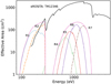 |
Fig. 1 Effective area curves of ROSAT and eROSITA. The global ROSAT effective area (solid pink line) is composed of six standard bands (labeled). The eROSITA broadband effective area curve (solid black line) combines cameras TM 1, 2, 3, 4, and 6. |
ROSAT standard band energy ranges.
2 Data processing
2.1 Calibration and processing logic
The calibrated eRASS1 data were processed with the standard eROSITA Science Analysis Software System pipeline (eSASS, version_201009, developed by the German eROSITA consortium; Brunner et al. 2022). The eSASS pipeline is made up of task chains that aim to produce different data products (Predehl et al. 2021). The EXP chain we used includes procedures of packing the telemetry data into staging areas, quality good time interval (GTI) creation, telescope-merged event files and images creation, bright pixel or track flagging, and exclusion.
In the eSASS pipeline calibration, the survey data are packed into distinct sky tiles according to the equatorial coordinates. Each sky tile is approximately 3.6 × 3.6 deg2 in size, with overlaps from the adjacent tiles.
The maps presented in this paper were generated by assembling the exposures and count images of each sky tile, which were then projected onto the full sky while preserving the surface brightness. The primary procedure was carried out by Python and eSASS tools. We especially thank J. Sanders for the contribution of the projection script. The maps in HealPix format were derived with healpy package1 (Zonca et al. 2019; Górski et al. 2005).
The creation of the surface brightness maps involves the following products and definitions: the counts map is the count of photons detected in the two-dimensional sky grids (i.e., per pixel: 9 arcmin2), and the exposure map is the representation of the observing time distribution on the sky. The exposure is defined as the sampling of the on-axis exposure time summed over the used telescope modules after correction for the vignetting function (see details in Sect. 2.2). The rates maps are the exposure-corrected maps obtained as the ratio of the counts map and the exposure map, and they are plotted in units of cts s−1.
Both the counts map and the exposure map were derived from the same event-files. The event files are the tables including all the information on the counts detected in a sky tile (i.e., energy, detection pattern, and arrival time) The prefiltering applied on the event files was shared with the different products. We note that we only included data from the five telescope modules (TMs) equipped with on-chip filters (i.e., TM1, 2, 3, 4, and 6), and we excluded data from TM 5 and 7 because they were affected by a light leak (Predehl et al. 2021).
2.2 Exposure and vignette correction
The exposure image was produced by the eSASS task expmap2. This setting produced the exposure corrected for the vignette and scaled to a single TM, as presented in Fig. 2. The correction factor for five TMs was implemented later in the effective area. eROSITA scans the sky along the great circles that pass the ecliptic poles and has a precession rate of 0.167 deg scan−1 (Predehl et al. 2021), with a field of view with a diameter of 1.03 deg. As a result of the survey strategy, the eROSITA exposure is characterized by a significant gradient across the sky. The cumulative on-axis observing time increases toward the ecliptic pole and reaches a maximum of ~40 ks/TM (20 ks/TM as a vignetted exposure in 0.2–0.6 keV), while it is only ~160 s/TM (90 s/TM as vignetted exposure) close to the ecliptic plane. The overall averaged and vignette-corrected exposure of eRASS1 in the 0.2–0.6 keV band in the western hemisphere is about 170 s/TM. A few small-scale fluctuations present in the exposure maps are caused by particular and time-dependent instrumental effects, such as TM switch off/on due to susceptibility in the camera electronics, variations in chopper settings, and so on.
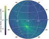 |
Fig. 2 eRASS1 unvignetted exposure in Galactic coordinates (solid grid) and ecliptic coordinates (dotted grid). Only the hemisphere (359.94423568 > l > 179.94423568 degrees) accessible to eROSITA DE consortium is presented. The color-coding corresponds to the accumulated integration time. The exposure was computed on-axis and averaged over the TMs (1, 2, 3, 4, and 6). |
2.3 Instrumental background
Accurate modeling and subtraction of the instrumental background is key to retrieving low surface brightness features in the maps. The instrumental background in the X-ray CCD detectors mostly results from electronic readout noise and charges caused by cosmic rays hitting the detector. Regular monitoring of the particle background has revealed that it is largely featureless (i.e., it can be modeled by smooth functions), it increases toward lower energies, and it flattens out at 2 keV. At higher energies (≥5 keV), the instrumental background dominates the incident flux in ~90% of the sky. Over the time period covered by eRASS1, this signal can be considered as time invariant (Freyberg et al. 2020).
Filter-wheel-closed data (FWC) are data taken with the filter wheel placed in closed position, preventing the camera from observing photons from the sky. The FWC model3 was used to estimate the instrumental background. eROSITA has performed several FWC observations during the performance verification (PV) phase and the survey at intervals. The PV FWC data have been published along with the eROSITA Early Data Release.
The instrumental background is unprocessed by the telescope optics and thus remains unaffected by the vignette. The instrument background can be characterized by the following formalism:
 (1)
(1)
where Rsky is the total count rate from X-ray sources (both diffuse and point-like), Ctotal is the total number of detected events, Tnonvig and Tvig are the unvignetted and vignette-corrected exposures, respectively, and RFWC is the instrumental background, which is built from the TM 1, 2, 3, 4, and 6 averaged FWC model. We also refer to the  ratio as the vignette coefficient.
We note that the characterization of the FWC data is under constant development and improvement by the eROSITA team. New background particle models will potentially improve in the time and CCD-temperature dependence of the FWC data.
2.4 Point source subtraction
To reveal the diffuse emission, the bright point sources need to be subtracted. We used the eRASS1 source catalog (Merloni et al. 2023), which contains about 850 000 point-source candidates. The uneven depth of the survey exposure naturally leads to nonuniform detection limits. To avoid the selection bias, only the sources above a rates threshold were subtracted in the diffuse maps. We defined the threshold on the count rates, which applies to two different purposes: in order to compare eROSITA maps with those of ROSAT, we retrieved the equivalent threshold from ROSAT (Table 2 in Snowden et al. 1997) and converted it into eROSITA observed rates, which corresponds to ~0.30 cts s−1 in the 0.6–2.3 keV band. A different threshold was instead chosen to include as many point sources as possible while retaining a uniform portion of the cosmic X-ray background from the entire sky. We determined the latter threshold as approximately the count rate of the faintest source that can be detected in the low-exposure regions (i.e., close to the ecliptic plane) of 0.03 ct/s in the 0.2–5.0 keV band.
We created a cheese-like mask in which the pixels above threshold (i.e., including point sources) were masked out. For each source, a circular mask with a predetermined radius was applied. The radius was scaled according to the flux of the source. The minimum radius was 100″ (about six times the half-energy width of eROSITA at 1.49 keV). The resulting masked regions were then filled with the average of the surrounding rates, estimated from the adjacent region where the signal to noise ratio (S/N) exceeds 2.
We note that all sources and features identified as extended sources in the eRASS1 catalog were preserved. Dust scattering can also produce a halo of diffuse emission around bright sources. This effect has been studied around different sources using the ROSAT data (Lamer et al. 2021; Jin et al. 2017; Predehl & Schmitt 1995) and is clearly detected by eROSITA as well (see Figs. F.1–F.4, the large halo surrounding Cir X-1, GX 349+2). We here retained these dust-scattering halos in the maps.
3 Broadband eROSITA diffuse emission maps
We present the first X-ray diffuse emission maps of eRASS1, available in Figs. E.1–E.5. The maps are represented in cylindrical projection, Galactic coordinates, in the energy bands: 0.2–0.4, 0.4–0.6, 0.6–1.0, 1.0–2.3, and 2.3–5.0 (keV). A spatially uniform contribution (in count rate units) of the instrumental background was subtracted from the maps, as described in Sect. 2.3. Adaptive smoothing (using S /N ≥ 20, unless otherwise stated) was applied for displaying purposes, while the unsmoothed version of the maps was used to quantify the properties reported in Table 2 and throughout the paper. The pixel resolution was set to 9 arcmin2 in all maps. This allows an average signal-to-noise ratio S/N > 1 in the 0.2–1.0 keV band maps (see Fig. C.2).
At different energies (i.e., different bands), the relative importance of the difference components that build the diffuse emission changes, as shown by the spectral study of the eROSITA Final Equatorial Depth Survey (eFEDS) region (Ponti et al. 2023).
In the softest band (0.2-0.4 keV), the entire hemisphere shows a significant contribution from the LHB, modeled as an unabsorbed collisionally ionized plasma at kT ~ 0.1 keV (Snowden et al. 1998). This emission must be situated within the local bubble because nonvanishing foreground emission toward the densest portions of the gas dark clouds is observed (Yeung et al. 2023). The morphology of the LHB was investigated using the ROSAT data (Liu et al. 2017). For comparison, we present in Fig. 3 the softest band (0.20–0.25 keV) map of the eRASS1 data. The high degree of similarity between the eROSITA and ROSAT maps implies that eROSITA has sufficient sensitivity to detect the very soft emission of the local plasma in the LHB.
A main emission source in 0.5–1.5 keV is the hot phase of the CGM of the Milky Way. This component has been fist recognized and detected by separation of the foreground and CXB components also through absorption by neutral clouds (Snowden et al. 2000; Pietz et al. 1998). In a similar way, this component is also detected by eROSITA and was studied (Locatelli et al. 2024) using the narrow-band data presented in a follow-up work of the present one (Zheng et al., in prep.). In the same band, the diffuse X-ray emission carries potential information on the heliospheric SWCX. Because of the time variability, this component can be isolated and studied by eROSITA (Dennerl et al., in prep.).
Above 0.7 keV, the emission from the CXB becomes the dominant component. At higher energies (E ≫ 1.5 keV), the integrated emission from faint and unresolved X-ray point sources (CXB, Gilli et al. 2007; Brandt & Yang 2021) dominates the emission. In addition, a minor but non-negligible contribution may come from patches of very hot interstellar medium (ISM; kT ≃ 0.7–1 keV; Ponti et al. 2023).
Global properties of the eRASS1 broadband map of the diffuse emission.
3.1 Global estimate of the surface brightness and the flux
In Table 2 we list the observed properties (surface brightness and total flux) of the diffuse emission detected in the broadband maps. We report the estimates for the western hemisphere (359.94423568 > l > 179.94423568) in the energy bands 0.2–0.4 keV, 0.4–0.6 keV, 0.6–1.0 keV, 1.0–2.3 keV, and 2.3–5.0 keV. The ECF were estimated and used to convert the observed count rates into surface brightness (S). The computation of the ECF involves knowledge of the eROSITA effective area and has to assume a spectral model. This was fixed as a power law with photon index of Γ = 2.0 absorbed by a column density of NHI = 5 × 1020 cm−2. The NH value stands for the median NH of the HI4PI survey (HI4PI Collaboration 2016). The computed ECF factors are also listed in Table 2.
We note that in the computation of all the properties reported in Table 2, we excluded well-known bright extended sources such as Vela supernova remnant (SNR), Sco X-1, and the Virgo cluster, which are bright enough to otherwise contaminate the result. On these sources, we applied circular masks with radii of 5, 4, and 3 deg, respectively.
We divided the western sky into five distinct patches I-V, based on quadrants, variations in absorption, and the predominant source of diffuse emissions (see Table 3): region I is representative of the Galactic plane, where the disk absorption has a significant impact. Region I spans the range of Galactic latitudes −15 to 15, roughly matching the NHI = 1021cm−2 contour of NH (HI4PI Collaboration 2016). Regions II and III represent the area of the northern and southern Galactic outflow (i.e., the eROSITA and Fermi bubbles), respectively. Regions IV and V are mostly free from either outflows or foregrounds. They sit in the northern and southern hemisphere, respectively, and lie closer to the Galactic anticenter. The absorption in regions IV and V has a smaller impact than for the rest of the western sky.
The averaged count rates, the surface brightness, and the total flux of regions I-V are presented in Fig. 4. In general, the large-scale surface brightness and flux peak in the 0.4-0.6 keV band. Below 0.4 keV, absorption due to the Galactic disk neutral material significantly reduces the observed flux. The uncertainties were derived as the statistical error.
We note that region II consistently shows the highest surface brightness of the regions up to 1 keV. The contrast is particularly noticeable in the 0.4–0.6 keV band, where region II exhibits a surface brightness of 2.75 × 10⁻¹¹erg s−1 cm−2 deg−2 keV−1. An enhancement toward the disk is well noticeable across the sky, especially in the harder bands, such as 2.3–5.0 keV. Most regions exhibit their highest surface brightness in the 0.4–0.6 keV band, while region I peaks in the 0.6–1.0 keV band, likely because of the heavy absorption as well as the contribution from bright point sources and the ISM in the Galactic plane.
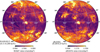 |
Fig. 3 Very soft band maps of ROSAT (R12: 0.11–0.284 keV, left) and eROSITA/eRASS1 (0.20–0.25 keV, right) in ZEA projection. The similarities between two surveys support the detectability of LHB with eROSITA. |
Regions and areas.
3.2 Absorption features
The observed soft-band diffuse X-ray maps clearly exhibit absorption as a significant suppression of the emission. In Fig. 5 we present examples of the effect of absorption on the X-ray spectrum. The decrement was modeled as an exponential with an exponent proportional to the column density NH of the absorbing material and an energy-dependent cross section σ ∝ E−3 (Balucinska-Church & McCammon 1992; Wilms et al. 2000; Locatelli et al. 2022).
The main contribution to the absorption comes from the Galactic interstellar medium. The cold phases encompassed by the ISM, including dust and molecules (dominantly H2) and mostly traced by neutral hydrogen, are in fact mainly concentrated in the Galactic plane (HI4PI Collaboration 2016), causing the most severe absorption of the X-ray intensity in region I. Toward the high galactic latitude sky, the photoelectric absorption becomes less important as the overall density distribution scales as sec|b| (Koutroumpa et al. 2006; Lallement et al. 2016). In addition, individual local clouds casts their X-ray shadows, as already probed by ROSAT (Snowden et al. 1991, 2000), and eROSITA (Yeung et al. 2023).
Figure 6 shows the X-ray emission along the Galactic plane from eRASS1 in RGB colors (Red: 0.2–0.5 keV. Green: 0.5–1.0 keV. Blue: 1.0–2.0 keV). The color-code is log-scaled and computed as  . We note that the point sources in Fig. 6 have been kept.
The dark band along the Galactic plane caused by absorption is one of the most noticeable features in eROSITA/eRASS1 maps. The most severe Galactic absorption is observed close to the direction of the Galactic center, where blue points to the hard-band photons, which alone pierce the foreground absorbing screen. The top panel of Fig. 6 clearly shows the sharp dimming of the emission as a function of Galactic latitude. The X-ray radiation dominant at high latitudes therefore has to originate behind the high column density regions in order to be obscured and to produce the darker patterns visible in region I. The gas clouds at medium latitudes can thus serve as useful distance constraints to the diffuse emission at the largest angular scales. To provide some reference values, by defining the on-plane absorption horizon as the distance from which the observed emission is reduced by a factor 1/e, an observer at the Sun would see through the disk up to ~0.1, 0.4, 0.8, and 3 kpc  in band 0.2–0.4 keV, 0.4–0.6 keV, 0.6–1.0 keV, and 1.0–2.3 keV, respectively. For comparison, the distance from the Solar System to the Galactic center is approximately 8.1 kpc (Reid & Brunthaler 2004).
In addition, the top panel shows an enhanced 0.5–1.0 keV emission that outlines the base of the hot plasma of the eROSITA bubbles. In the middle panel of Fig. 6, the 0.2–0.5 keV emission and the 0.5–1.0 keV become relatively mixed and even, with the blue of 1.0–2.3 keV photons highlighting the hard point sources in the disk. In the direction of the Galactic anticenter (bottom panel of Fig. 6), the emission is dominated by soft emission of 0.2–0.5 keV, especially in the region of bright SNRs. The Monogem Ring (Knies et al., in prep.) is visible as an extended (~10 deg) arc-shaped emission. The blue diffuse emission above 1.0 keV is barely noticeable, while the brightest peak corresponds to hard point sources.
In Fig. 7 the contours from the column density map taken from the full-sky neutral hydrogen survey (HI4PI Collaboration 2016) overlap the 0.2–0.4 keV eRASS1 map. The RASS data are affected by systematic uncertainties that can be reached by the apparent stripes, while the eRASS data are nearly smooth in brightness transition. We show three NH I contour levels as the imprints of the Galactic absorption gradient: 2 × 10²⁰, 5 × 10²⁰, and 1 × 1021 cm−2. The anticorrelation of the column density and the X-ray emission is clear. At energies above several kilo electronvolts, the emission from the Galactic disk is only marginally absorbed (see also Figs. E.4 and E.5).
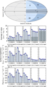 |
Fig. 4 Configuration and observed properties of the sky patches. We divided the eROSITA DE sky into five parts as listed in Table 3. The hatched gray regions in the count-rate histogram show the level of the particle background. We converted count rates into surface brightness assuming a power-law model S ∝ E−Γ with Γ = 2 and absorption as in Table 3. The surface brightness and flux estimations use the ECFs reported in Table 2. |
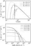 |
Fig. 5 Effect of absorption on the X-ray spectrum. Top panel: energy dependence of the absorption spectrum. The unabsorbed spectrum is defined as Fv = v−2. The labeled lines show column densities matching the contours in Fig. 7. Bottom panel: effect of NHI on the broadband flux. The vertical lines show the threshold at which Fv decreases by a factor |

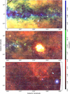 |
Fig. 6 Maps of the Galactic disk from eRASS1 survey in RGB colors (Red: 0.2–0.5 keV. Green: 0.5–1.0 keV. Blue: 1.0–2.0 keV). The color brightness scales as |

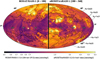 |
Fig. 7 NH1 contours overlaid onto the eROSITA soft-band images. The western sky l = [180, 360] shows the eROSITA/eRASSl data in the 0.2–0.4 keV band mirrored with respect to Galactic longitude l = 0. The eastern sky l = [0, 180] shows the ROSAT/RASS R12 (0.11-0.284 keV) band map. The contour superimposed are the column density from the HI4PI survey: NH1 = 2 × 10²⁰ (dotted), 5 × 10²⁰ (solid), and 1 × 1021 cm−2 (dot dashed). |
4 Comparison with ROSAT X-ray diffuse emission
We compared the eROSITA broadband maps to the ROSAT diffuse background maps from (Snowden et al. 1997)4. The ROSAT maps were corrected for particle background and scattered solar X-rays along with the long-term enhancements (LTE) detected by ROSAT. A few regions that were severely impacted by the effect of single reflection (i.e., the photons are only reflected once before they reach the sensor) were also manually removed in the version of the ROSAT maps presented in this work.
The left and right columns in Figs. F.1–F.4 present the count rates of the diffuse emission observed by eROSITA and ROSAT, respectively. The maps are projected with the zenith equal area (ZEA) projection and use Galactic coordinates in the ROSAT R4–R7 energy bands (Figs. F.1–F.4, respectively; see Table 1 and Snowden et al. 1997 for the definitions of the energy ranges). Identical sources yield different count rates in the eROSITA and ROSAT data due to their different effective areas (see Fig. 1). We employed energy-to-counts conversions in the relevant energy range with the assumption of a power law v−2 spectrum to convert rates into fluxes. The color bars in Figs. F.1–F.4 were set to the same flux values to ensure that features with constant flux appeared with similar colors in both maps.
A remarkable match of the X-ray emissions detected by eROSITA (eRASS1) and ROSAT (RASS) is immediately noticeable. Prominent large-scale features exhibit comparable levels of brightness in both measurements. The sites showing the largest deviation between the maps form stripes along ecliptic longitudes in the ROSAT maps. These are caused by the enhanced particle background, induced by solar activity, at the orbit/position of the ROSAT spacecraft, compared to the relatively quiet environment of SRG/eROSITA (i.e., the L2 point). Additional residual effects close to the passage of ROSAT through the South Atlantic Anomaly are also present (Snowden & Freyberg 1993). Another obvious discrepancy is visible around Sco X-1 (i.e., the brightest point source in the X-ray sky), where the contribution due to the single reflection is brighter in the eROSITA data. With their large photon-collecting area, the eROSITA eRASS1 maps are able to probe the diffuse emission more deeply. In Fig. D.1, a discrete but large number of extended sources (i.e., galaxy clusters) is now also recognizable in the eROSITA maps, but they could not be distinguished in the ROSAT maps.
4.1 Method
To assess the consistency of the eROSITA and ROSAT measurements, we compared the observed count rates. To do this, the maps were smoothed on a common grid to an angular resolution of 0.839 deg25. In order to avoid assuming the spectral shape of the emission, the comparison was carried out in count rates rather than flux. Different sources are characterized by different spectra. ECFs computed for each pixel, depending on the assumed spectrum, would be required to take this into account.
The observed count rates were determined by the numbers of photons within each pixel divided by the exposure (vignette corrected). To make the observed eROSITA count rates directly comparable to the ROSAT ones, we split each broad energy band (R2, R4–R7) into ten narrower energy bands (this number of narrow bands still preserves S/N > 3). For a sufficiently small energy range, the converted eROSITA count rate becomes equivalent to that of ROSAT regardless of the spectrum of the source. We calculated the eROSITA count rate for each sub-band and multiplied it by the ratio of the effective areas of the two different instruments. Finally, we summed the contribution from all narrow energy bands to present the equivalent rate in the broad band. In this way, the observed eROSITA count rate was converted into a ROSAT equivalent count rate, becoming directly comparable to that of ROSAT.
The procedure is formalized by Eq. (2), where Ei represents the differential energy bins in each band,
 (2)
(2)
For completeness and reproducibility, we note that we applied the following corrections before computing the converte count rates for ROSAT and eROSITA:
- i)
Large-scale rebinning of ROSAT data: the removal of particle background, scattered solar foreground, and long-term enhancement in the publicly available ROSAT soft X-ray maps (Snowden et al. 1997) leaves pixels with negative or unusually high count rates. These spurious pixels are mostly found along the ecliptic longitude. By rebinning the maps into larger pixels, the high-value pixels are naturally removed.
- ii)
S/N screening. We used the uncertainty (sigma) map of ROSAT as a quality criterion to screen out pixels with S/N < 3, mostly tracing pixels affected by a systematic large uncertainty. For example, applying S/N > 3 to the R4 map preserves 98.3% of the data points, with 15.7% of them holding S/N > 10. The effect of filtering the data with higher S/N is more noticeable in band R7.
- iii)
Single reflection: due to the single reflection caused when ROSAT and eROSITA scan over very bright sources (e.g. Sco X-1), the observed flux can experience a systematic increase due to the photons coming from outside the field of view (about 1 deg in diameter). These spurious photons have interacted with the mirror system only once before ending up on the detector plane. The single reflection is stronger in eROSITA than in ROSAT because of the extra baffle of eROSITA and the large reflection angle. This effect is visible around Sco X-1 and other bright point sources. We masked these sources with a 5° radius circle. As visible in Fig. A.1C, the filtering on single reflections affects the typical count rates in the 0.5 < Rro < 1.0 and 0.8 < Rero < 2.0 of ROSAT and eROSITA, respectively.
4.2 Results
The converted eROSITA count rates (i.e., equivalent to ROSAT; see Eq. (2)) are plotted against the ROSAT rates in Fig. 8 for the R4–R7 bands. The density peak at fixed eROSITA count rate is marked by a blue dot with the y(x) error bars showing the converted eROSITA and ROSAT uncertainty, respectively. The uncertainty in the eROSITA maps is at least five times smaller than in the ROSAT, at all rates. The rate (Poissonian) uncertainty of the eROSITA and ROSAT counts is also applied around the 1:1 relation in the shaded gray region.
Figure 8 shows and evident correlation between the two instruments in all bands in the 0.05–10 cts s−1 deg−2 rate range. The 1:1 relation is generally well matched by the data, with a scatter in addition. As shown by the yellow glow in the plots, most of the data are in the 0.1−0.3 cts s−1 deg−2 rate range. The converted rates of eROSITA in R4 and R5 appear to be slightly lower than the ROSAT rates in the entire range of values, pointing to a small systematic shift. In R6 and R7, the rates agree with the 1:1 relation, but they appear to be more scattered in R7. R7 in particular holds more data at high rates that are affected by large deviations from the 1:1 relation compared the other bands. For the higher photon energies of R7, the Galactic diffuse emission becomes fainter and the CXB contributes most at the faint end, which follows the 1:1 relation better.
The lower panels in Fig. 8 show the residuals of the data with respect to the 1:1 relation. The residuals are defined as |eRO − RO|σtot, where σtot refers to the combined Poisson uncertainty of both eROSITA and ROSAT. The residuals averaged over the western sky are 1.079, 1.073, 1.424, and 1.240 in R4–R7, respectively. Of the four bands, R6 thus shows the largest scatter. Data with lower rates are in general closer to the 1:1 relation, considering their larger uncertainty, while the bright end deviates more from the 1:1 line in all bands.
The blue points summarize the trend followed by the data. We fit these peak density points with a linear relation. The result is shown by the dash-dotted blue lines in all the panels of Fig. 8. The best-fit relations between the converted eROSITA rates (y) and the ROSAT rates (x) are 0.905x − 0.022, 0.880x − 0.01, 0.900x + 0.003 and 0.992x − 0.020 for R4−R7, respectively. From these fits, we find that the converted eROSITA rates are lower than the ROSAT rates by about ~12%, except for the R7 band. We note that we only fit the densest location instead of the whole data because a small number of extreme outliers had a very small statistical uncertainty because we did not include any systematic uncertainty in the computation. Thus, the statistical uncertainty underestimates the total uncertainty by an amount comparable to the (unknown) systematic, potentially arising from the removal of solar activity enhancement and subtraction of the particle background.
In Fig. 9 (see Figs. F.1–F.4 for zoom-in versions) we show the rate maps of ROSAT (Rro, left column) and the converted eROSITA (Rero2ro, central column) rate maps for direct visual inspection. After the conversion, these maps show theoretically comparable rate measurements. The places where eROSITA is brighter than ROSAT indicate the points above the 1:1 correlation found in Fig. 8 and vice versa. The coherent patches producing the highest residuals are clearly visible in the left and right column of Fig. 9. The converted eROSITA maps are visually similar to the ROSAT rates, with most of the diffuse structures being similar. The residual maps show that the most prominent difference appears as bright stripes along ecliptic longitudes, indicating a dependence on the observing time. These stripes arise from the subtraction of the ROSAT long-term enhancement and short flares, done empirically. The traces can be also seen directly from the cleaned ROSAT maps in the left column. The dependence on the observation time can explain the difference at fainter count rates, and also the intercept at zeropoint of the fitted relations: The eROSITA/eRASS1 was in fact carried out during a period of relatively quiescent solar activity. However, the 12% discrepancy at the brighter end of R4–R6 is not well understood. Considering the different instrument design and space environments, the origin of the (small) discrepancy between the coefficient and a 1:1 relation might be convoluted as well. This systematic difference is small, however, and we speculate that it is accounted for by including calibration differences, which were not tested in this work.
In Fig. 10 we show the rate comparison in the R4 band in detail (top panels). They show no obvious offset at the zeropoint. The resemblance of the data from the two observations is seen down to very low rates (≃0.05 cts s−1 deg−2), corroborating the quality of the systematic background calibration at this extent. In the bottom panels of Fig. 10, we show the scatter of the ROSAT data. By taking a slice of pixels at about 0.53 cts s−1 deg−2 of the converted eROSITA rates (cyan area in the top right panel), we draw the distribution of their ROSAT rates (bottom left panel) and compute the full width at half maximum (FWHM) of the distribution. In general, in two observations detecting the same flux with high statistics and no systematics (i.e., Poisson uncertainty only), the rate distribution should be a Gaussian with FWHM = 2.3548σ, where σ is the standard deviation of the Gaussian. We thus wish to compare the width of the distribution, converted into σ, to the intrinsic ROSAT uncertainty. In the bottom right panel of Fig. 10, we show the measured σ at fixed eROSITA equivalent rates for all rates. We note that the σ (solid blue line) grows together with the ROSAT uncertainty (dashed black line). We find that σ is about 1.25 times of the ROSAT uncertainty for all bands (see the dotted black line). The eROSITA uncertainty was ignored in this computation as negligible compared to the ROSAT uncertainty. According to this comparison, the eROSITA data agree with the ROSAT within 1.25 times the ROSAT uncertainty. They are thus consistent.
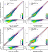 |
Fig. 8 Rate comparison of diffuse emission maps of eROSITA/eRASSl and ROSAT/RASS in log scale. Each data point shows the rates from 0.83 deg2 sky region (NSIDE 64). The converted eROSITA rates were calculated from Eq. (2) to be equivalent to the ROSAT response. The screening is by S/N > 3 in the ROSAT data. The color corresponds the density of the data in this plot. The navy points with error bars mark the density peak in the eROSITA rates with a 1σ confidence. The navy dash-dotted line is the best fit of the densest points. The lines with a slope of 1 and 0.75 (1.25) and zero intercept are shown with the solid red line and dashed black lines, respectively. The intrinsic Poisson uncertainty level corresponding to 1 pix size is shown by the gray shadow. |
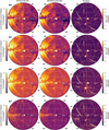 |
Fig. 9 Visual comparison of the data. ROSAT/RASS maps (left column), the converted eROSITA maps (middle column), and the residual maps (right column) of the diffuse emission observed in four bands. The converted count rates are the rates scaled with the ROSAT PSPC response. The deviation is defined as the |

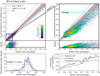 |
Fig. 10 Detailed view of the ROSAT and eROSITA comparison in the R4 energy band. Top left: same as Fig. 8 (top left panel), shown in linear scale. Top right: zoom-in on the rate range 0−0.8cts s−1 deg−2. Bottom left: schematic distribution of the ROSAT rates taken from the redefined eROSITA rate range (shown in cyan in the top right panel). The blue line is the smoothed number density that falls into this rate channel, from which the FWHM is measured. Bottom right: equivalent a and the uncertainty reported by ROSAT with respect to the eROSITAconverted rates. The ROSAT uncertainty is dominated by Poissonian noise. The red triangle shows the equivalent σ from the bottom left panel. The 1.25 times ROSAT uncertainty is shown with a dashed line for comparison. |
5 Large-scale sources of diffuse emission
5.1 The case of the eROSITA bubbles
Because of the extraordinary concordance between the ROSAT and eROSITA maps, it is reasonable to question why the eROSITA bubbles were not immediately recognized on the basis of the ROSAT maps (Snowden et al. 1997). We note that the main features that allowed Predehl et al. (2020) to recognize the eROSITA bubbles are their hourglass shape, which comes from the fourfold symmetry around the Galactic center, which comes about through the detection of faint diffuse emission at high Galactic latitudes.
Based on the ROSAT maps, the existence of a bright X-ray spur northeast of the Galactic center was clearly recognized, which is now known as the North Polar Spur (Iwan 1980; Sofue & Reich 1979). By virtue of the eROSITA maps, it is evident that the continuation of the North Polar Spur forms a loop, with a fainter edge on the northwestern side of the Galactic center (Predehl et al. 2020). Considerable complexity along the north-western edge of the bubbles was already recognized based on the ROSAT maps in particular. Through the attempt of decomposition for the diffuse ROSAT emission in Freyberg (1994), some emission features from local diffuse features were possibly separated. Figure 11 shows a feature at 1, b ~ (315, 20) that was initially attributed to a local SNR. Even in the higher-quality eROSITA maps, this foreground emission complicates the identification of the northwestern edge of the eROSITA bubbles, which is well defined, but rather faint at high Galactic latitudes (b ≥ 30°), while its edge becomes unclear at lower latitudes. Therefore, it is not surprising that the northwest edge of the bubble was not recognized in the ROSAT data.
The southwest edge of the eROSITA bubbles is instead much clearer. They can clearly be delineated from few degrees below the Galactic disk all the way to |b| ~ 50° (Predehl et al. 2020). However, the very clear edge is severely confused in the ROSAT map. This location on the sky corresponds to the passage of ROSAT through the South Atlantic Anomaly, which is characterized by an elevated background and induces a significantly shallower exposure in the ROSAT maps at that location (see Fig. 11). Therefore, it is not surprising that the faint southeast edge of the eROSITA bubbles has not been recognized in the lower-sensitivity ROSAT maps.
Considering that the southeast edge of the eROSITA bubbles was not detected because of its faintness, its southwest edge was not noticed because of the higher background and shorter exposure related with the passage of ROSAT through the South Atlantic Anomaly, its northwest edge was confused by large-scale features (which was attributed to a local supernova remnant) and the North Polar Spur was thought to be a uniquely a local feature, it is not surprising that the footprint of the eROSITA bubbles could not be recognized on the basis of the ROSAT maps. However, studies (Kataoka et al. 2018) have already anticipated the existence of the eROSITA bubbles with high certainty from the gamma-ray observation.
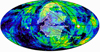 |
Fig. 11 Foreground components in the ROSAT map with the eROSITA bubble contour overlaid. This foreground maps was built by Freyberg (1994), who modeled and separated the foreground emissions from RASS map. The resulting maps are shown with the angular resolution of 0.2°. We overlay the contour of eROSITA bubbles (defined from 0.6–1.0 keV band) as a white translucent area. |
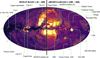 |
Fig. 12 Finding chart of the all-sky diffuse emission. The western sky l = [180, 360] is shown with the eROSITA/eRASSl data in the 0.4–0.6 keV band. The eastern sky l = [0, 180] is shown with the ROSAT/RASS R4 (0.44–1.01 keV) band map. The green marks show the location of large projected structures, including known supernova remnants, the Large and Small Magellanic Clouds, and some extended clusters and galaxy superclusters. The color bar has been arbitrarily chosen to match the dynamic ranges of the maps. |
5.2 Other sources
Direct visual examination of the eRASS1 maps revealed a variety of structures of diffuse emission. In this section, we enumerate the prominent diffuse emission features and structures in the maps and briefly characterize them in order to provide an idea of the diffuse emission sky. For this purpose, Fig. 12 shows the locations and extent of large projected coherent patches of diffuse emission in the soft X-ray band. In the eastern Galactic hemisphere (l = [0, 180]), we show the ROSAT R4 map of 0.44–1.01 keV, and in the western Galactic hemisphere (l = [180, 360]), we show the eROSITA data in the 0.4–0.6 keV band.
Within the Galactic plane, only local emission (≤200 pc) is not damped by the high absorption. At intermediate Galactic latitudes, large-scale diffuse emission generated by the hot gas in the halo of the Milky Way and supernova remnants becomes noticeable. Large-scale features such as the Monogem Ring at l, b ~ (200, 15) (Knies et al. 2018, and in prep.), the Orion-Eridanus superbubble at l, b ~ (210, −40), an expanding superbubble filled with X-ray emitting plasma rising from the Galactic plane (Joubaud et al. 2019; Burrows et al. 1993; Heiles et al. 1999), the Antlia supernova remnant at l, b ~ (280, 23) (Knies et al., in prep.), the recently discovered Hoinga at l, b ~ (249.5, 24.5) (Becker et al. 2021), and the nearby SNR l, b ~ (320, 20) are clearly distinguished.
The comparison of eROSITA maps with the corresponding ROSAT maps additionally reveals brightness and/or flux changes for variable X-ray sources, such as novae and X-ray binaries. For example, the X-ray transient nova Musca 1991 (G295-7) was evident in the ROSAT maps through all bands, but it is not detectable (or is significantly fainter) in the eROSITA maps (see also Figs. F.1–F.4).
6 Summary
We presented the diffuse X-ray emission maps of the eRASS1 data in different energy bands from 0.2 to 8.0 keV. We demonstrated the capability of eROSITA to detect faint diffuse emission sources, including the LHB, the Galactic halo, various SNRs, the ISM, and the CXB through soft to hard energies. We reported the observed rates, surface brightness, and total flux in the western Galactic hemisphere. The energy resolution of eROSITA allows a detailed investigation of the Galactic diffuse plasma, with a narrower energy selection than for the ROSAT data.
The data from eROSITA/eRASS1 were quantitatively compared with the ROSAT maps in the ROSAT standard bands, after taking into account the instrumental background and response efficiency. The visual inspection of eRASS1 and RASS maps already shows strong similarities in the morphology of the diffuse emission in the whole hemisphere. Through a quantitative comparison, the fit of the densest data sample shows that eROSITA observes count rates consistent with ROSAT, with a weak systematic tendency to lower rates. The correlation coefficient is ~90% in R4–R6, and it is ~99% in R7, while the scatter of the data is about 1.25 times of the measurement uncertainty in all bands. We attribute the small residual deviation from the 1:1 relation as potentially caused by the different calibration procedures and by the subtraction of emission induced by solar activity. We sketched the all-sky atlas of the prominent diffuse emission structures present in the literature and detected by eROSITA and provided an overview of the known diffuse sources in the soft X-ray sky.
The following eROSITA all-sky surveys will provide more details for sources of diffuse emission, allowing us to improve the characterization of the various plasma components and environment of the Milky Way, nearby galaxies, and the extragalactic sky. The broadband data products presented in this work will soon be made available in a dedicated eROSITA repository during the eRASS1 data release.
Acknowledgements
This work is based on data from eROSITA, the soft X-ray instrument aboard SRG, a joint Russian-German science mission supported by the Russian Space Agency (Roskosmos), in the interests of the Russian Academy of Sciences represented by its Space Research Institute (IKI), and the Deutsches Zentrum fur Luft- und Raumfahrt (DLR). The SRG spacecraft was built by Lavochkin Association (NPOL) and its subcontractors, and is operated by NPOL with support from the Max Planck Institute for Extraterrestrial Physics (MPE). The development and construction of the eROSITA X-ray instrument was led by MPE, with contributions from the Dr. Karl Remeis Observatory Bamberg & ECAP (FAU Erlangen-Nuernberg), the University of Hamburg Observatory, the Leibniz Institute for Astrophysics Potsdam (AIP), and the Institute for Astronomy and Astrophysics of the University of Tubingen, with the support of DLR and the Max Planck Society. The Argelander Institute for Astronomy of the University of Bonn and the Ludwig Maximilians Universität Munich also participated in the science preparation for eROSITA. The eROSITA data shown here were processed using the eSASS software system developed by the German eROSITA consortium. This research made use of Astropy (http://www.astropy.org), a community-developed core Python package for Astronomy (Astropy Collaboration 2013, 2018). Some of the results in this paper have been derived using the healpy and HEALPix packages. We acknowledge financial support from the European Research Council (ERC) under the European Union’s Horizon 2020 research and innovation program Hot- Milk (grant agreement No 865637).
Appendix A Correction tracking
In Sec. 4 we present different corrections that aimed to prepare theeROSITA data for a quantitative comparison with the ROSAT data, as presented in Fig.8. In Fig.A.1 we provide versions of the data in with each correction is applied or is not applied.
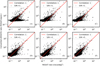 |
Fig. A.1 Detailed view of the ROSAT and eROSITA comparison in the R7 energy band. (A)–(B): Horizontal branch deviation (shown in A) without the negative values. Instead, keeping and smoothing them results in the improved plot (B). This corresponds to the correction “ROSAT elliptic longitudinal stripes” in the text. (B)–(C): We masked out the Sco X-1 in plot (C) because the single-reflection effect is stronger in eROSITA. By this, we removed about 30 data points, which exceed than 1 - 1 relation as for the result. This corresponds to the correction in “Light reflection”. (C)–(D): Particle background of eROSITA was subtracted in this step to match the ROSAT data, which are free of particle background. (D)–(E)–(F): Selection over ROSAT S/N. Increasing the S/N threshold sharpens the 1 - 1 relation especially in fainter samples. This step corresponds to the “uncertainty selection.” |
Appendix B Projection distortion
For different displaying purposes, we used different projections in this paper. In Fig. B.1 we show the distortion effect of projections over eRASS1: 0.6–1.0 keV map. The cylindrical perspective (CYP) projection does not conserve the pixel area at different coordinates. The maps in CYP projection were corrected for the weight maps to recover the surface brightness.
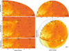 |
Fig. B.1 Distortions of the squared 3x3 degree2 sky tiles (in tangential projection around the center of the sky tile) when they are differently projected. The other projections represented here are CYP, CEA, AIT, ZEA, and orthographic (SIN) projections. Only the northwest Galactic hemisphere is shown. In a nonequal area projection (e.g., CYP), the shape of a region is distorted and the projected area of each equal sky tile is not conserved. The sky tiles at higher Galactic latitudes appear to be stretched. |
Appendix C Determining the map resolution
The maps are presented in a pixel size of 3 arcmin. This setup was chosen to balance the S/N in the bright and faint sky area. Because of the scanning strategy, the exposure accumulates at the ecliptic poles (see the exposure, vignette corrected, at different energies in Fig. C.1). According to the exposure, the significance of the detection is calculated in Fig. C.2. The y-axis reports the average S/N over half the sky. The 9 arcmin2 pixel satisfies the S/N > 1 in all the broadband maps.
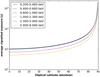 |
Fig. C.1 Average exposure (vignette corrected) per TM in different energy bands of eRASS1 as a function of ecliptic latitude. |
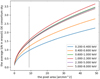 |
Fig. C.2 Average significance in different eRASS1 energy bands as a function of the pixel size. The vertical dashed line is set at 9 arcmin2, used in this work. |
Appendix D Contribution of clusters in eRASS1
The sensitivity of eROSITA enables us to probe the sky to a larger depth. Hence, faint extended sources such as galaxy clusters can be distinguished. As the main scientific goal of eROSITA, the detection of galaxy clusters candidates is expected to extend their census by more than one order of magnitude. Fig.D.1 (point sources subtracted) shows a still considerable number of radiating objects throughout the sky, even in the Galactic plane. Most of them are galaxy clusters that are classified in an upcoming eRASS1 cluster catalog. In contrast to eROSITA, ROSAT does not observe the faintest end of the cluster luminosity function (i.e., the largest amount), due to small count statistics. In the field we show here, ~ 300 clusters candidates are present. After further subtraction of these extended sources, a smoother large-scale diffuse emission can be obtained.
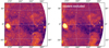 |
Fig. D.1 eRASS1 0.44-1.01 keV band with and without galaxy cluster candidates (left and right). Point sources were subtracted from both maps as described in Sec. 2.4. The cluster candidates are extracted from the extended sources presented in the eRASS1 catalog (Merloni et al. 2023) |
Appendix E High-resolution eROSiTA eRASS1 broadband maps
Here we present the gallery of high-resolution (pixel size of 3 arcmin) eRASS1 broadband maps of bands 0.2–0.4 keV, 0.4–0.6 keV, 0.6–1.0 keV, 1.0–2.3 keV, and 2.3–5.0 keV. The final maps are available in fits and HealPix format. More details of the map processing can be found in Sec.2.
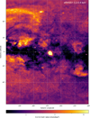 |
Fig. E.1 Broadband 0.2–0.4 keV eRASS1 map in CYP. The color bar shows the range 1.0 – 9.0 cts s−1 deg−2 in log scale. An adaptive smoothing with S/N ≥ 20 is used. The minimum threshold is set at the instrumental background of this energy band. |
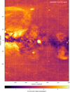 |
Fig. E.2 Broadband 0.4–0.6 keV eRASS1 map in CYP. The color bar shows the range 1.0 – 14.0cts s−1 deg−2 in log scale. An adaptive smoothing with S/N ≥ 20 is used. The minimum threshold is set at the instrumental background of this energy band. |
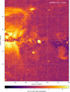 |
Fig. E.3 Broadband 0.6–1.0 keV eRASS1 map in CYP. The color bar shows the range 1.0 – 22.0 cts s−1 deg−2 in log scale. An adaptive smoothing with S/N ≥ 20 is used. The minimum threshold is set at the instrumental background of this energy band. |
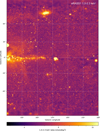 |
Fig. E.4 Broadband 1.0–2.3 keV eRASS1 map in CYP. The color bar shows the range 2.5 – 18.0 cts s−1 deg−2 in log scale. An adaptive smoothing with S/N ≥ 20 is used. The minimum threshold is set at the instrumental background of this energy band. |
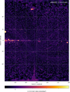 |
Fig. E.5 Broadband 2.3–5.0 keV eRASS1 map in CYP. The color bar shows the range 5.5 – 13.0 cts s−1 deg−2 in log scale. An adaptive smoothing with S/N ≥ 20 is used. The minimum threshold is set at the instrumental background of this energy band. |
Appendix F Additional maps of eROSITA and ROSAT
Additional plots are shown here for a detailed comparison of the eROSITA and ROSAT count rates. By placing the sextant section of the eRASS1 and RASS maps in parallel, the comparison can be verified by direct visual inspection.
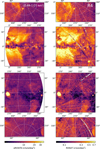 |
Fig. F.1 Count-rate maps of eROSITA (left column) and ROSAT (right column) in the R4 band (0.44–1.01 keV). A ZEA projection is used. North is up. The log-scaled color bar covers 90% of the dynamic pixel range. |
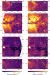 |
Fig. F.2 Count-rate maps of eROSITA (left column) and ROSAT (right column) in the R5 band (0.56–1.21 keV). A ZEA projection is used. North is up. The log-scaled color bar covers 90% of the dynamic pixel range. |
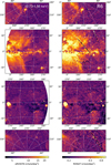 |
Fig. F.3 Count-rate maps of eROSITA (left column) and ROSAT (right column) in the R6 band (0.73–1.56 keV). A ZEA projection is used. North is up. The log-scaled color bar covers 90% of the dynamic pixel range. |
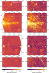 |
Fig. F.4 Count-rate maps of eROSITA (left column) and ROSAT (right column) in the R7 band (1.05–2.04 ke V). A ZEA projection is used. North is up. The log-scaled color bar covers 90% of the dynamic pixel range. |
References
- Astropy Collaboration (Robitaille, T. P., et al.) 2013, A&A, 558, A33 [NASA ADS] [CrossRef] [EDP Sciences] [Google Scholar]
- Astropy Collaboration (Price-Whelan, A. M., et al.) 2018, AJ, 156, 123 [Google Scholar]
- Balucinska-Church, M., & McCammon, D. 1992, ApJ, 400, 699 [Google Scholar]
- Becker, W., Hurley-Walker, N., Weinberger, C., et al. 2021, A&A, 648, A30 [NASA ADS] [CrossRef] [EDP Sciences] [Google Scholar]
- Brandt, W. N., & Yang, G. 2021, Handbook of X-ray and Gamma-ray Astrophysics, eds. C. Bambi, & A. Santangelo (Singapore: Springer) [Google Scholar]
- Brunner, H., Liu, T., Lamer, G., et al. 2022, A&A, 661, A1 [NASA ADS] [CrossRef] [EDP Sciences] [Google Scholar]
- Burrows, D. N., Singh, K. P., Nousek, J. A., Garmire, G. P., & Good, J. 1993, ApJ, 406, 97 [NASA ADS] [CrossRef] [Google Scholar]
- Freyberg, M. 1994, PhD Thesis, Ludwig-Maximilians University of Munich, Germany [Google Scholar]
- Freyberg, M., Perinati, E., Pacaud, F., et al. 2020, SPIE Conf. Ser., 11444, 1144410 [Google Scholar]
- Gilli, R., Comastri, A., & Hasinger, G. 2007, A&A, 463, 79 [NASA ADS] [CrossRef] [EDP Sciences] [Google Scholar]
- Górski, K. M., Hivon, E., Banday, A. J., et al. 2005, ApJ, 622, 759 [Google Scholar]
- Heiles, C., Haffner, L. M., & Reynolds, R. J. 1999, ASP Conf. Ser., 168, 211 [Google Scholar]
- HI4PI Collaboration (Ben Bekhti, N., et al.) 2016, A&A, 594, A116 [NASA ADS] [CrossRef] [EDP Sciences] [Google Scholar]
- Iwan, D. 1980, ApJ, 239, 316 [NASA ADS] [CrossRef] [Google Scholar]
- Jin, C., Ponti, G., Haberl, F., & Smith, R. 2017, MNRAS, 468, 2532 [NASA ADS] [CrossRef] [Google Scholar]
- Joubaud, T., Grenier, I. A., Ballet, J., & Soler, J. D. 2019, A&A, 631, A52 [NASA ADS] [CrossRef] [EDP Sciences] [Google Scholar]
- Kataoka, J., Sofue, Y., Inoue, Y., et al. 2018, Galaxies, 6, 27 [Google Scholar]
- Kerp, J., Burton, W. B., Egger, R., et al. 1999, A&A, 342, 213 [Google Scholar]
- Knies, J. R., Sasaki, M., & Plucinsky, P. P. 2018, MNRAS, 477, 4414 [NASA ADS] [CrossRef] [Google Scholar]
- Koutroumpa, D., Lallement, R., Kharchenko, V., et al. 2006, A&A, 460, 289 [NASA ADS] [CrossRef] [EDP Sciences] [Google Scholar]
- Lallement, R., Vergely, J. L., Puspitarini, L., et al. 2015, Mem. Soc. Astron. Italiana, 86, 626 [NASA ADS] [Google Scholar]
- Lallement, R., Snowden, S., Kuntz, K. D., et al. 2016, A&A, 595, A131 [NASA ADS] [CrossRef] [EDP Sciences] [Google Scholar]
- Lallement, R., Capitanio, L., Ruiz-Dern, L., et al. 2018, A&A, 616, A132 [NASA ADS] [CrossRef] [EDP Sciences] [Google Scholar]
- Lamer, G., Schwope, A. D., Predehl, P., et al. 2021, A&A, 647, A7 [NASA ADS] [CrossRef] [EDP Sciences] [Google Scholar]
- Liu, W., Chiao, M., Collier, M. R., et al. 2017, ApJ, 834, 33 [Google Scholar]
- Locatelli, N., Ponti, G., & Bianchi, S. 2022, A&A, 659, A118 [NASA ADS] [CrossRef] [EDP Sciences] [Google Scholar]
- Locatelli, N., Ponti, G., Zheng, X., et al. 2024, A&A, 681, A78 [NASA ADS] [CrossRef] [EDP Sciences] [Google Scholar]
- McCammon, D., Almy, R., Apodaca, E., et al. 2002, ApJ, 576, 188 [NASA ADS] [CrossRef] [Google Scholar]
- Merloni, A., Predehl, P., Becker, W., et al. 2012, ArXiv e-prints [arXiv:1209.3114] [Google Scholar]
- Merloni, A., Liu, T., Ramos-Ceja, M. E., et al. 2023, A&A, submitted [Google Scholar]
- Pietz, J., Kerp, J., Kalberla, P. M. W., et al. 1998, A&A, 332, 55 [NASA ADS] [Google Scholar]
- Ponti, G., Zheng, X., Locatelli, N., et al. 2023, A&A, 674, A195 [NASA ADS] [CrossRef] [EDP Sciences] [Google Scholar]
- Predehl, P., & Schmitt, J. H. M. M. 1995, A&A, 500, 459 [Google Scholar]
- Predehl, P., Sunyaev, R. A., Becker, W., et al. 2020, Nature, 588, 227 [CrossRef] [Google Scholar]
- Predehl, P., Andritschke, R., Arefiev, V., et al. 2021, A&A, 647, A1 [EDP Sciences] [Google Scholar]
- Reid, M. J., & Brunthaler, A. 2004, ApJ, 616, 872 [Google Scholar]
- Snowden, S. L., & Freyberg, M. J. 1993, ApJ, 404, 403 [NASA ADS] [CrossRef] [Google Scholar]
- Snowden, S. L., Mebold, U., Hirth, W., Herbstmeier, U., & Schmitt, J. H. M. 1991, Science, 252, 1529 [NASA ADS] [CrossRef] [Google Scholar]
- Snowden, S. L., Egger, R., Freyberg, M. J., et al. 1997, ApJ, 485, 125 [Google Scholar]
- Snowden, S. L., Egger, R., Finkbeiner, D. P., Freyberg, M. J., & Plucinsky, P. P. 1998, ApJ, 493, 715 [NASA ADS] [CrossRef] [Google Scholar]
- Snowden, S. L., Freyberg, M. J., Kuntz, K. D., & Sanders, W. T. 2000, ApJS, 128, 171 [NASA ADS] [CrossRef] [Google Scholar]
- Sofue, Y., & Reich, W. 1979, A&AS, 38, 251 [NASA ADS] [Google Scholar]
- Sunyaev, R., Arefiev, V., Babyshkin, V., et al. 2021, A&A, 656, A132 [NASA ADS] [CrossRef] [EDP Sciences] [Google Scholar]
- Truemper, J. 1982, Adv. Space Res., 2, 241 [Google Scholar]
- Tumlinson, J., Peeples, M. S., & Werk, J. K. 2017, ARA&A, 55, 389 [Google Scholar]
- Wilms, J., Allen, A., & McCray, R. 2000, ApJ, 542, 914 [Google Scholar]
- Yeung, M. C. H., Freyberg, M. J., Ponti, G., et al. 2023, A&A, 676, A3 [NASA ADS] [CrossRef] [EDP Sciences] [Google Scholar]
- Zonca, A., Singer, L., Lenz, D., et al. 2019, J. Open Source Softw., 4, 4 [Google Scholar]
Input parameters withvignetting = YES, withmergedmaps = YES, withweights = NO, withdetmaps = YES.
Here the FWC of version c020_v1.0 was used. More details can be found at the eROSITA Early data release website: https://erosita.mpe.mpg.de/edr/eROSITAObservations/EDRFWC
Available at: https://heasarc.gsfc.nasa.gov/docs/rosat/survey/sxrb/#maps
This angle corresponds to an Healpix pixel using nside = 64.
All Tables
All Figures
|
Fig. 1 Effective area curves of ROSAT and eROSITA. The global ROSAT effective area (solid pink line) is composed of six standard bands (labeled). The eROSITA broadband effective area curve (solid black line) combines cameras TM 1, 2, 3, 4, and 6. |
| In the text | |
|
Fig. 2 eRASS1 unvignetted exposure in Galactic coordinates (solid grid) and ecliptic coordinates (dotted grid). Only the hemisphere (359.94423568 > l > 179.94423568 degrees) accessible to eROSITA DE consortium is presented. The color-coding corresponds to the accumulated integration time. The exposure was computed on-axis and averaged over the TMs (1, 2, 3, 4, and 6). |
| In the text | |
|
Fig. 3 Very soft band maps of ROSAT (R12: 0.11–0.284 keV, left) and eROSITA/eRASS1 (0.20–0.25 keV, right) in ZEA projection. The similarities between two surveys support the detectability of LHB with eROSITA. |
| In the text | |
|
Fig. 4 Configuration and observed properties of the sky patches. We divided the eROSITA DE sky into five parts as listed in Table 3. The hatched gray regions in the count-rate histogram show the level of the particle background. We converted count rates into surface brightness assuming a power-law model S ∝ E−Γ with Γ = 2 and absorption as in Table 3. The surface brightness and flux estimations use the ECFs reported in Table 2. |
| In the text | |
|
Fig. 5 Effect of absorption on the X-ray spectrum. Top panel: energy dependence of the absorption spectrum. The unabsorbed spectrum is defined as Fv = v−2. The labeled lines show column densities matching the contours in Fig. 7. Bottom panel: effect of NHI on the broadband flux. The vertical lines show the threshold at which Fv decreases by a factor |
| In the text | |
|
Fig. 6 Maps of the Galactic disk from eRASS1 survey in RGB colors (Red: 0.2–0.5 keV. Green: 0.5–1.0 keV. Blue: 1.0–2.0 keV). The color brightness scales as |
| In the text | |
|
Fig. 7 NH1 contours overlaid onto the eROSITA soft-band images. The western sky l = [180, 360] shows the eROSITA/eRASSl data in the 0.2–0.4 keV band mirrored with respect to Galactic longitude l = 0. The eastern sky l = [0, 180] shows the ROSAT/RASS R12 (0.11-0.284 keV) band map. The contour superimposed are the column density from the HI4PI survey: NH1 = 2 × 10²⁰ (dotted), 5 × 10²⁰ (solid), and 1 × 1021 cm−2 (dot dashed). |
| In the text | |
|
Fig. 8 Rate comparison of diffuse emission maps of eROSITA/eRASSl and ROSAT/RASS in log scale. Each data point shows the rates from 0.83 deg2 sky region (NSIDE 64). The converted eROSITA rates were calculated from Eq. (2) to be equivalent to the ROSAT response. The screening is by S/N > 3 in the ROSAT data. The color corresponds the density of the data in this plot. The navy points with error bars mark the density peak in the eROSITA rates with a 1σ confidence. The navy dash-dotted line is the best fit of the densest points. The lines with a slope of 1 and 0.75 (1.25) and zero intercept are shown with the solid red line and dashed black lines, respectively. The intrinsic Poisson uncertainty level corresponding to 1 pix size is shown by the gray shadow. |
| In the text | |
|
Fig. 9 Visual comparison of the data. ROSAT/RASS maps (left column), the converted eROSITA maps (middle column), and the residual maps (right column) of the diffuse emission observed in four bands. The converted count rates are the rates scaled with the ROSAT PSPC response. The deviation is defined as the |
| In the text | |
|
Fig. 10 Detailed view of the ROSAT and eROSITA comparison in the R4 energy band. Top left: same as Fig. 8 (top left panel), shown in linear scale. Top right: zoom-in on the rate range 0−0.8cts s−1 deg−2. Bottom left: schematic distribution of the ROSAT rates taken from the redefined eROSITA rate range (shown in cyan in the top right panel). The blue line is the smoothed number density that falls into this rate channel, from which the FWHM is measured. Bottom right: equivalent a and the uncertainty reported by ROSAT with respect to the eROSITAconverted rates. The ROSAT uncertainty is dominated by Poissonian noise. The red triangle shows the equivalent σ from the bottom left panel. The 1.25 times ROSAT uncertainty is shown with a dashed line for comparison. |
| In the text | |
|
Fig. 11 Foreground components in the ROSAT map with the eROSITA bubble contour overlaid. This foreground maps was built by Freyberg (1994), who modeled and separated the foreground emissions from RASS map. The resulting maps are shown with the angular resolution of 0.2°. We overlay the contour of eROSITA bubbles (defined from 0.6–1.0 keV band) as a white translucent area. |
| In the text | |
|
Fig. 12 Finding chart of the all-sky diffuse emission. The western sky l = [180, 360] is shown with the eROSITA/eRASSl data in the 0.4–0.6 keV band. The eastern sky l = [0, 180] is shown with the ROSAT/RASS R4 (0.44–1.01 keV) band map. The green marks show the location of large projected structures, including known supernova remnants, the Large and Small Magellanic Clouds, and some extended clusters and galaxy superclusters. The color bar has been arbitrarily chosen to match the dynamic ranges of the maps. |
| In the text | |
|
Fig. A.1 Detailed view of the ROSAT and eROSITA comparison in the R7 energy band. (A)–(B): Horizontal branch deviation (shown in A) without the negative values. Instead, keeping and smoothing them results in the improved plot (B). This corresponds to the correction “ROSAT elliptic longitudinal stripes” in the text. (B)–(C): We masked out the Sco X-1 in plot (C) because the single-reflection effect is stronger in eROSITA. By this, we removed about 30 data points, which exceed than 1 - 1 relation as for the result. This corresponds to the correction in “Light reflection”. (C)–(D): Particle background of eROSITA was subtracted in this step to match the ROSAT data, which are free of particle background. (D)–(E)–(F): Selection over ROSAT S/N. Increasing the S/N threshold sharpens the 1 - 1 relation especially in fainter samples. This step corresponds to the “uncertainty selection.” |
| In the text | |
|
Fig. B.1 Distortions of the squared 3x3 degree2 sky tiles (in tangential projection around the center of the sky tile) when they are differently projected. The other projections represented here are CYP, CEA, AIT, ZEA, and orthographic (SIN) projections. Only the northwest Galactic hemisphere is shown. In a nonequal area projection (e.g., CYP), the shape of a region is distorted and the projected area of each equal sky tile is not conserved. The sky tiles at higher Galactic latitudes appear to be stretched. |
| In the text | |
|
Fig. C.1 Average exposure (vignette corrected) per TM in different energy bands of eRASS1 as a function of ecliptic latitude. |
| In the text | |
|
Fig. C.2 Average significance in different eRASS1 energy bands as a function of the pixel size. The vertical dashed line is set at 9 arcmin2, used in this work. |
| In the text | |
|
Fig. D.1 eRASS1 0.44-1.01 keV band with and without galaxy cluster candidates (left and right). Point sources were subtracted from both maps as described in Sec. 2.4. The cluster candidates are extracted from the extended sources presented in the eRASS1 catalog (Merloni et al. 2023) |
| In the text | |
|
Fig. E.1 Broadband 0.2–0.4 keV eRASS1 map in CYP. The color bar shows the range 1.0 – 9.0 cts s−1 deg−2 in log scale. An adaptive smoothing with S/N ≥ 20 is used. The minimum threshold is set at the instrumental background of this energy band. |
| In the text | |
|
Fig. E.2 Broadband 0.4–0.6 keV eRASS1 map in CYP. The color bar shows the range 1.0 – 14.0cts s−1 deg−2 in log scale. An adaptive smoothing with S/N ≥ 20 is used. The minimum threshold is set at the instrumental background of this energy band. |
| In the text | |
|
Fig. E.3 Broadband 0.6–1.0 keV eRASS1 map in CYP. The color bar shows the range 1.0 – 22.0 cts s−1 deg−2 in log scale. An adaptive smoothing with S/N ≥ 20 is used. The minimum threshold is set at the instrumental background of this energy band. |
| In the text | |
|
Fig. E.4 Broadband 1.0–2.3 keV eRASS1 map in CYP. The color bar shows the range 2.5 – 18.0 cts s−1 deg−2 in log scale. An adaptive smoothing with S/N ≥ 20 is used. The minimum threshold is set at the instrumental background of this energy band. |
| In the text | |
|
Fig. E.5 Broadband 2.3–5.0 keV eRASS1 map in CYP. The color bar shows the range 5.5 – 13.0 cts s−1 deg−2 in log scale. An adaptive smoothing with S/N ≥ 20 is used. The minimum threshold is set at the instrumental background of this energy band. |
| In the text | |
|
Fig. F.1 Count-rate maps of eROSITA (left column) and ROSAT (right column) in the R4 band (0.44–1.01 keV). A ZEA projection is used. North is up. The log-scaled color bar covers 90% of the dynamic pixel range. |
| In the text | |
|
Fig. F.2 Count-rate maps of eROSITA (left column) and ROSAT (right column) in the R5 band (0.56–1.21 keV). A ZEA projection is used. North is up. The log-scaled color bar covers 90% of the dynamic pixel range. |
| In the text | |
|
Fig. F.3 Count-rate maps of eROSITA (left column) and ROSAT (right column) in the R6 band (0.73–1.56 keV). A ZEA projection is used. North is up. The log-scaled color bar covers 90% of the dynamic pixel range. |
| In the text | |
|
Fig. F.4 Count-rate maps of eROSITA (left column) and ROSAT (right column) in the R7 band (1.05–2.04 ke V). A ZEA projection is used. North is up. The log-scaled color bar covers 90% of the dynamic pixel range. |
| In the text | |
Current usage metrics show cumulative count of Article Views (full-text article views including HTML views, PDF and ePub downloads, according to the available data) and Abstracts Views on Vision4Press platform.
Data correspond to usage on the plateform after 2015. The current usage metrics is available 48-96 hours after online publication and is updated daily on week days.
Initial download of the metrics may take a while.