| Issue |
A&A
Volume 681, January 2024
|
|
|---|---|---|
| Article Number | A78 | |
| Number of page(s) | 18 | |
| Section | Galactic structure, stellar clusters and populations | |
| DOI | https://doi.org/10.1051/0004-6361/202347061 | |
| Published online | 19 January 2024 | |
The warm-hot circumgalactic medium of the Milky Way as seen by eROSITA
1
Max-Planck-Institut für Extraterrestrische Physik (MPE), Giessenbachstrasse 1, 85748 Garching bei München, Germany
2
INAF – Osservatorio Astronomico di Brera, Via E. Bianchi 46, 23807 Merate, LC, Italy
e-mail: This email address is being protected from spambots. You need JavaScript enabled to view it.
3
Dr. Karl Remeis Observatory, Erlangen Centre for Astroparticle Physics, Friedrich-Alexander-Universität Erlangen-Nürnberg, Sternwartstraße 7, 96049 Bamberg, Germany
Received:
31
May
2023
Accepted:
14
October
2023
Abstract
The first all-sky maps of the diffuse emission of high ionization lines observed in X-rays by SRG/eROSITA provide an excellent probe for the study of the warm-hot phase (T ∼ 106 K) of the circumgalactic medium (CGM) of the Milky Way. In this work, we analyze the O VIII line detected in the first eROSITA All-Sky Survey data (eRASS1). We fit a sky map made in a narrow energy bin around this line with physical emission models embedded in a 3D geometry in order to constrain the density distribution of the warm-hot gas around the Galaxy, with a focus on mid and high (absolute) Galactic latitudes. By masking out the eROSITA bubbles and other bright, extended foreground sources, we find that an oblate geometry of the warm-hot gas (T ≡ 0.15 − 0.17 keV), flattened around the Galactic disk with scale height zh ∼ 1 − 3 kpc, best describes the eRASS1 O VIII map, with most of the observed emission shown as being produced within a few kiloparsecs from the Sun. The additional presence of a large-scale warm-hot spherical halo, while providing a minor contribution to the X-ray emission, accounts for the high O VII absorption column densities detected with XMM-Newton as well as most of the baryon budget of the CGM of the Milky Way. To date, the eROSITA data carry the greatest amount of information and detail of the O VIII CGM intensities, allowing for a significant reduction in the statistical uncertainties of the inferred physical parameters.
Key words: Galaxy: general / X-rays: diffuse background
© The Authors 2024
 Open Access article, published by EDP Sciences, under the terms of the Creative Commons Attribution License (https://creativecommons.org/licenses/by/4.0), which permits unrestricted use, distribution, and reproduction in any medium, provided the original work is properly cited.
This article is published in open access under the Subscribe to Open model.
Open access funding provided by Max Planck Society.
1. Introduction
The largest contribution to the gas mass budget of galaxies is expected to be retained in a hot phase in the halo that extends over scales that are comparable to their virial radius Rvir, with temperature T ∼ 105 − 107 K (White & Rees 1978; Tumlinson et al. 2017). The presence of these hot gas halos results from the infall of intergalactic material onto the spines and nodes of the dark matter structure of the Universe (i.e., the cosmic web), from the ∼megaparsec scales down to smaller-scale peaks (∼100 kpc) corresponding to the galactic dark matter halos. The infalling gas bulk motions and collisions power stationary shock waves at the boundaries of the potential wells. These stationary shocks compress and heat the gas inside the well up to a temperature similar (but not necessarily equal; see Lochhaas et al. 2023) to the virial temperature Tvir ∝ Rvir/Mvir ∼ 105 − 107 K usually computed at Rvir ≡ R200 (see Oppenheimer et al. 2018; Nelson et al. 2018, and references therein). The medium enclosed within this radius and found outside the stellar disk of a galaxy is usually defined as the circumgalactic medium (CGM).
In this warm-hot gas phase of the CGM, collisions between the gas atoms dominate the energy exchange between them and in turn the overall ionization of the atomic species. The collisional ionization equilibrium hypothesis thus provides a theoretical framework to compute the expected brightness of the ionization lines of the warm-hot gas phase (Smith et al. 2001). Such a phase has been observed as all-sky diffuse X-ray emission since about three decades already (e.g., Kuntz & Snowden 2000, based on ROSAT all-sky X-ray survey data). High ionization lines of species like C IV, O VII, O VIII, or Ne IX are the most common states, and their presence has been confirmed around external galaxies by several independent probes, including via the absorption features they produce along the lines of sight toward bright active galactic nuclei (Gupta et al. 2012; Miller & Bregman 2013; Nicastro et al. 2023; Das et al. 2019a,b); via their associated emission lines studies (Forman et al. 1985; O’Sullivan et al. 2001; Yao et al. 2009; Henley & Shelton 2010; Bogdán et al. 2013; Miller & Bregman 2015; Goulding et al. 2016; Faerman et al. 2017; however, see the potential biases pointed out by Zheng et al. 2020); by detecting diffuse emission around external galaxies (Strickland et al. 2004; Tüllmann et al. 2006; Li et al. 2017; Hodges-Kluck et al. 2018); via stacking experiments over a large sample of distant galaxies revealing the presence of a layer of hot gas distributed closely within and around galactic stellar disks (Anderson et al. 2015; Comparat et al. 2022; Chadayammuri et al. 2022). In the context of the Milky Way (MW), spectral evidence of both warm-hot T ≃ 0.2 − 0.3 keV and hot T ≃ 0.7 − 1 keV gas phases have been reported (Yoshino et al. 2009; Gupta et al. 2012; Nakashima et al. 2018; Das et al. 2019a,b; Kaaret et al. 2020; Bhattacharyya et al. 2023; Ponti et al. 2023; Bluem et al. 2022) and similar components have also been recently associated to the Large Magellanic Cloud (Gulick et al. 2021).
The same set of evidence, however, may also suggest an alternative scenario in which the heated gas is expelled from the stellar disk from the explosions of supernovae by mechanical or radiative energy feedback. The gas outflowing from the stellar disk may then cool, precipitate, and fall back onto the disk, creating a re-cycling of the gas and powering new episodes of star formation (Shapiro & Field 1976; Bregman 1980). Given the sensitivity of X-ray experiments to particle density, usually increasing toward the inner portions of galactic halos, this scenario is a complementary alternative to the gravitational infall, providing an explanation for the presence of a hot gas phase around galaxies.
The current picture for the MW indicates the presence of both types of scenarios (i.e., gas accreted from the large-scale environment versus outflowing from the Galactic disk), with a component distributed in a disk-like geometry extending roughly a few kiloparsecs above and below the Galactic plane and producing most of the observed X-ray CGM emission while a large-scale (∼100 − 300 kpc) halo is also present but provides a minor contribution to the emission (Nakashima et al. 2018; Kaaret et al. 2020; Qu & Bregman 2019; Bluem et al. 2022). The halo component, however, would contain most of the mass associated with the hot gas phase due to its enormous volume.
A crucial aspect in studies of the diffuse emission of the MW is to cover large portions of the sky with sufficient spatial resolution in order to discriminate the morphology of sources and distinguish components at the same time. The sky fraction sampled by instruments with good spatial and spectral resolution (e.g., XMM-Newton, Chandra) is small due to the relatively small field of view (compared to 4π sr). In this respect, the ROSAT mission (Snowden & Schmitt 1990; Snowden et al. 1997) operational in the 1990s set a milestone by producing the first all-sky X-ray map. However, the spectral resolution of ROSAT, providing five broadbands from 0.1 to 2.4 keV, prevented studies of single emission lines as well as an easy identification of the different sources of diffuse emission in a given energy band. More recently, the HaloSat instrument provided a larger coverage at high Galactic latitudes with a spatial resolution of 10 deg and relatively good spectral resolution (85 eV at 0.68 keV, Kaaret et al. 2019). The best figure of merit exploiting a high survey speed and a sufficient spectral resolution, combined with a high spatial resolution, has finally been reached by the extended ROentgen Survey with an Imaging Telescope Array (eROSITA) instrument onboard the Spectrum-Roentgen-Gamma (SRG) space observatory, launched in July 2019. eROSITA is a space X-ray telescope featuring a large effective area from 0.2 to 8 keV (comparable to that of XMM-Newton in the 0.3−2 keV band) in combination with a large field of view (∼1 deg2), high spatial resolution (∼30 arcsec), and an instrumental energy resolution of ∼80 eV at 1 keV (Merloni et al. 2012; Sunyaev et al. 2021; Predehl et al. 2021). For the first time, these features combined allow the soft X-ray background (0.2−1 keV) to be broken down into its components, including the hot CGM of the MW, in both spectra and high-resolved images.
In this paper, we present the analysis of the first ever O VIII half-sky1 emission lines maps (Zheng et al., in prep.) aimed at constraining the density distribution and overall geometry of the warm-hot CGM of the MW. The spectral analysis performed on the eROSITA Final Equatorial Depth Survey (eFEDS; Brunner et al. 2022), a deep ∼140 deg2 field at moderate Galactic latitudes (20° < b < 40°, Ponti et al. 2023, and references therein), provides us with information on the temperature and metal content of the detected CGM phases. Adopting this information, we derive the X-ray emission of simple 3D geometrical models for the CGM density and look for the model that best describes the narrowband map of the detected O VIII emission line.
In Sect. 2 we briefly summarize the data reduction extensively presented in Zheng et al. (2023, and in prep.). In Sect. 3, we describe the components used to model the line emission and the method used to fit the CGM geometry to the data. In Sect. 4, we present our main results, and in Sect. 5 we discuss them in the context of the literature. In Sect. 6, we summarize our results and draw our conclusions.
2. Data
The main emphasis in this work is given to the modeling of the line emission detected in the first all-sky survey of the eROSITA data (eRASS1). However, a comprehensive analysis of the hot CGM of the MW, which is the scientific driver of our research, cannot ignore additional and complementary information retrieved by independent missions or methods. Among the data sets presented below, the eRASS1 maps retain the highest statistical power thanks to the orders-of-magnitude larger sample size.
We analyzed the data from the first eROSITA All-Sky Survey of the eROSITA_DE consortium. We exploited images of the count rate per pixel generated from the original event files of eROSITA in different narrow energy bands as presented in Zheng et al. (in prep.; please also refer to Zheng et al. 2023 for details on the image production). The narrowband encompasses the [0.614−0.694] keV range and is named after the most prominent emission line included within the range, namely, the O VIII line (∼0.654 keV). The energy range was fixed to 80 eV near the line centroid in order to approximately account for the eROSITA energy resolution at around the corresponding energies (Predehl et al. 2021). The O VIII band map was created using the eROSITA Science Analysis Software System (eSASS) version 020 and is shown in Fig. 1. The eROSITA data were checked and validated against the ROSAT data (Zheng et al. 2023).
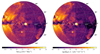 |
Fig. 1. eRASS1 O VIII intensity data used in this work. Data are shown using a Zenith Equal Area projection in the Galactic coordinate reference frame and centered at (l, b) = (270, 0) deg throughout this work. We note that the left panel includes the contribution from the eROSITA instrumental background, and the sky flux was processed through the effective area of eROSITA. The right panel shows the same map, but the instrumental background has been subtracted, leaving the signal from the sky (see Eq. (2)). We divided the sky signal by the eROSITA effective area to obtain the surface brightness of the physical sky signal in line units (L.U. = ph s−1 cm−2 sr−1). |
The eRASS1 data feature a highly nonuniform exposure across the sky, producing a direction-dependent sensitivity threshold to point-source detection. Removing point-source emission homogeneously (including active galactic nuclei) and taking the subtraction correctly into account in the modeling of the cosmic X-ray background (CXB) is not trivial. We thus decided to subtract only the brightest point sources detected in the 0.2−2.3 keV band (Merloni et al., in prep.) above a flux of 10−12 erg s−1 cm−2. This high threshold allowed us to remove bright source contamination in the maps while keeping the CXB contribution uniform across the sky. We converted the original FITS maps in HEALPix format with the use of the HEALPy Python library (Zonca et al. 2019). The HEALPix maps, defined to provide sky area units of equal surface (Górski et al. 2005), were used in our analysis, whereas a Zenith Equal Area projection is used throughout this work for displaying purposes only.
In addition, we considered a catalog of O VII Kα absorption column densities retrieved thanks to the higher spectral resolution of the XMM-Newton Reflection Grating Spectrometer (Bregman & Lloyd-Davies 2007; Miller & Bregman 2013). The column density N of the absorption lines is directly proportional to (the integral of) the density of the medium N ∝ nL (whereas emission intensity goes as ∝n2L). For this reason, O VII absorption data are particularly relevant to constraining lower density plasma located at large distances from the Sun.
2.1. eRASS1 data selection
The eRASS1 data cover the western Galactic sky. We show the O VIII narrow energy band map in Fig. 1. Several large angular scale features and sources show up in the map (e.g., eROSITA bubbles, the Eridanus-Orion superbubble, the Monogem Ring supernova remnant, etc.). These extended sources would bias our analysis if kept in the data, and thus the analysis of the hot CGM of the MW presented in this work required exclusion of the photons coming from these sources. We therefore selected all pixels within 2σb of Fig. 1 (left panel), where σb represents the root-mean-square value computed at every latitude b in the 220 deg < l < 250 deg stripe at the same latitude b. The longitude range considered is in fact clear from extended foreground sources, as is evident from Fig. 1.
In addition, we excluded all regions holding total hydrogen column densities NH > 1.6 × 1021 cm−2. Overestimation of the total hydrogen column density may in fact affect lines of sight in which not all of the emission comes from behind the absorption layer. This effect may become more prominent closer to the disk, where column density is also higher. The column density threshold of NH > 1.6 × 1021 cm−2 fixes the bias on the absorbed emission model in the O VIII band to be less than 30% for any absorbed source for assumed NH values within a factor +50% of the true value. The selected lines of sight used in our analysis are shown in Fig. D.1. They are mostly found at |b|> 15 deg. Clusters of galaxies from the MCXC catalog (Piffaretti et al. 2011) were also masked up to twice their R500 reported value. The regions excluded from the resulting mask well approximate either the presence of extended foreground sources or high column density regions (i.e., the Galactic disk). The final selected area used for the analysis presented in this work amounts to approximately one-third of the western sky (i.e., ∼6.6 k deg2).
2.2. Ubiquitous background and foreground components
The selected data represents what is commonly referred to as the X-ray sky background. The spectrum extracted in the eFEDS region is shown in Fig. 5 of Ponti et al. (2023) together with the proposed best-fits of the data. By looking at their model components, the diffuse background in the 0.6−0.7 keV band includes the emission of the hot CGM (blue line), whose 3D structure we aim to analyze. Other components that we aim to isolate are also present, namely, the instrumental background (INST; black line) and the CXB (magenta line). In softer energy bands (e.g., O VII, 0.5−0.6 keV) the addition of the Local Hot Bubble emission (LHB; red line) and the potential presence of the solar wind charge exchange (SWCX; cyan line) complicate the analysis. Despite O VII being the most prominent CGM emission line, in this work, we do not analyze the 0.5−0.6 keV energy range due to the limited knowledge about the detailed morphology of the LHB and SWCX components. Nonetheless, both the LHB and SWCX components are found to only provide a minor contribution in the O VIII band (see Appendices B and C for details on the modeling). We then considered the O VIII band as the main driver of our results. Study of the O VIII/O VII line ratio is expected to provide deeper insight into the temperature distribution across the sky, provided that degeneracy between the various components building the O VII emission can be correctly separated. The study of the O VII line, however, goes beyond the scope of the analysis presented here and will be addressed in a future work.
In addition to a warm-hot medium, a hotter plasma component (kT ∼ 107 K) was introduced in the eFEDS spectral analysis to model excess emission found at ∼1 keV. This component may produce emission that is also in the O VIII band, although with an intensity comparable to the LHB and SWCX components, amounting to only 1 − 2% of the total intensity in this band. Given the very little information available on the shape and properties of this component, as well as the minor contribution in the O VIII band, for simplicity we left it out of our analysis.
We thus describe the CGM intensity as
 (1)
(1)
 (2)
(2)
![Mathematical equation: $$ \begin{aligned}&I_{\rm add}(\boldsymbol{s},E) = I_{\rm CXB}(E)\,e^{-\sigma (E) N_{\rm H}(\boldsymbol{s})} + \left[I_{\rm LHB}(\boldsymbol{s},E) + I_{\rm SWCX}(\boldsymbol{s},E)\right], \end{aligned} $$](/articles/aa/full_html/2024/01/aa47061-23/aa47061-23-eq3.gif) (3)
(3)
where s ≡ (l, b) is expressed in Galactic coordinates and E is the photon energy. The exponential term models the absorption by neutral material in the interstellar medium (ISM), with σ being the absorption cross section of X-ray radiation (Balucinska-Church & McCammon 1992), assuming photospheric abundances (Lodders 2003), and NH(l, b) as the total hydrogen column density along a given line of sight (see Appendix A). The terms in square brackets are considered in the analysis of the O VIII band eRASS1 data but only provide minor contributions to the intensity (see the appendix for further details).
Below we provide descriptions of the components other than the CGM with the aim of modeling and subtracting them from the eRASS1 intensity in the different narrow energy ranges.
2.2.1. Instrumental particle background
The spurious contribution of charges produced in the camera sensor (CCD) was computed by collecting data with the filter wheel in the closed position (FWC). The resulting particle spectrum has been described and modeled in Predehl et al. (2021), and the models for all of the telescope modules (TM) have been made available2 through the eROSITA Early Data Release (EDR) of the Calibration and Performance Verification (CalPV) phase (see also Yeung et al. 2023). We built the particle spectrum in units of counts per second, per square degree, per kiloelectronvolt [cts s−1 deg−2 keV−1] by summing over the FWC models for the only TMs used to produce our line images (i.e., TM 1, 2, 3, 4 and 6). The spectrum was then multiplied by the pixel area in square degrees and integrated in the line energy range of interest to obtain the expected count rate. The background was observed to be significantly constant over the sky, and we thus assumed single values of 0.122 cts s−1 deg−2. From the scatter in the TMs data, we estimated a fractional error of 5% on the instrumental noise component, measured on a square degree scale.
2.2.2. Cosmic X-ray background
We modeled the cosmic X-ray background as a sum of two broken power-laws (Smith et al. 2007; Henley & Shelton 2012), as this model is able to describe the steepening of the summed spectrum of the sources building up the extragalactic background below 2 keV (Hasinger et al. 1993). The first power-law breaks at Eb = 0.4 keV and evolves from ∝E−1.9 for E ≤ 0.4 keV to E−1.6 for E ≥ 0.4 keV. At E > 1.2 keV. After a second break, the function is described by E−1.45. The CXB spectrum normalization at 1 keV is 10.9 ph s−1 cm−2 sr−1 keV−1. After multiplying by the effective area in the line energy range and integrating over the spectrum, we estimated CXB’s contribution to be 0.29 ph s−1 deg−2 in the O VIII band. In addition, the CXB is expected to be absorbed by the neutral material in the ISM, as it is generated in the background of the ISM with respect to an observer from Earth. We thus applied the absorption factor e−σ(E)NH(s, E) to this component (see Eq. (3)). Due to absorption, the final (additive) CXB contribution to the line intensity is dependent on the line of sight. We attributed a fractional error of 4% to the knowledge of the CXB count rate on a square degree scale (Revnivtsev et al. 2003).
3. Model of the eRASS1 CGM maps
3.1. Physical models
By “modeling the warm-hot CGM”, we refer to either modeling an extended spherical halo component or an oblate or disk-like distribution, usually referred to as the corona. The term “corona” is used across different fields of astronomy and plasma physics, and it is usually linked to the presence of diffuse and highly ionized plasma. For the hot phase of the CGM of galaxies, “corona” has been used in connection with a disk-shape morphology that is closer to stellar or ISM scale lengths than to virial radius scales. If the link between a spherical large-scale morphology and the presence of diffuse ∼virialized gas is well motivated and supported by other observations (Henley & Shelton 2013; Miller & Bregman 2013; although see also Lochhaas et al. 2021), in general, observing a nonspherical, disk-like component of the emission does not directly imply a diffuse volume-filling plasma as its source. We thus prefer the geometrical term “disk-like” rather than “corona”. This semantic difference allows us to separate the direct results of our analysis, which are mostly based on geometrical arguments and are to some extent independent of the actual physics, from the physical picture derived after assuming a diffuse plasma as the source of the emission. The relative importance of the two classes of models (i.e., spherical halo and disk-like), as well as the sources of the emission, motivated us to try different recipes to first describe the geometry of the soft X-ray emission described by the eROSITA data.
3.2. Thermo-chemistry
We modeled the gas of the Galactic halo as an isothermal distribution with T = 1.7 × 10⁶ K (kT = 0.15 keV). This assumption on the temperature is supported by the analysis of the eROSITA spectrum in the eFEDS field (Ponti et al. 2023) and tightly constrained by the ratio between the line intensities of highly ionized species (Henley & Shelton 2012). The large background region available in the eFEDS field allowed us to reach detailed energy calibration of the O VII line in the eRASS1 data, showing a value consistent with being dominated by emission from the recombination line (Ponti et al. 2023). This corroborates the assumption of a collisionally ionized plasma in thermal equilibrium for the warm-hot component. The G-ratio3 and the spectral fit performed by Ponti et al. (2023) using an APEC model also provide consistent and independent temperature estimates of kT = 0.15 − 0.17 keV (respectively including or not including an SWCX component). Different studies find a warm-hot temperature component at slightly different temperatures around kT ≃ 0.2 keV (McCammon et al. 2002; Yoshino et al. 2009; Gupta et al. 2021; Das et al. 2021; Kaaret et al. 2020; Bhattacharyya et al. 2023); however, systematic shifts may arise depending on the number of gas phases used to fit the spectra (Bluem et al. 2022). Previous studies have also found a small observed scatter at high Galactic latitudes (ΔkT ≃ 0.023 keV, Kaaret et al. 2020). In addition, we tested a model with kT = 0.225 keV and Z = 0.3 Z⊙ to assess potential systematic uncertainties in the fit results. We note that a constant temperature profile is also expected for any virialized halo following a total mass profile M(< r)∝r, such as the one derived by assuming a Navarro-Frenk-White dark matter profile (Navarro et al. 1997) in the theoretical framework of ΛCDM cosmology. Important deviations from the virial temperature may nonetheless be common depending on the amount of turbulence, bulk motions, magnetic fields, and accelerated cosmic rays in one galaxy. A uniform metal abundance Z = 0.1 Z⊙ was also assumed for the halo (Ponti et al. 2023).
3.2.1. Geometry: Spherical virialized halo
In the extended halo model the density of the hot material is most simply described by a spherical β model
![Mathematical equation: $$ \begin{aligned} n(r) = n_0 \left[1 + \left(\frac{r}{r_0}\right)^2 \right]^{-\frac{3}{2}\beta }, \end{aligned} $$](/articles/aa/full_html/2024/01/aa47061-23/aa47061-23-eq4.gif) (4)
(4)
where r is the distance to the Galactic center, n0 and r0 describe the flattening of the inner profile, and β describes the roll-off of the density at large radii. In fact, since in practice we masked out most directions in the quarter slab close to the Galactic center (|l|≥270 deg), due to either foreground structures or high absorption, we considered a simpler formula for the β model by setting the limit of the model to large radii. Small radii are in fact probed mostly by directions close to the Galactic center, and these directions are excluded from our analysis. The asymptotic formula also reduces the number of degrees of freedom as
 (5)
(5)
This treatment allowed us to ignore the degeneracy between the central parameters and to potentially obtain a more robust estimate for β, which is key to correctly inferring the mass of the baryons.
3.2.2. Geometry: Oblate disk-like component
In an alternative scenario, the X-ray emission can be produced by a hot corona powered by outflows of hot gas driven by supernovae explosions surrounding the stellar disk or by an unresolved population of Galactic sources distributed in and around the disk. Both imply a nonspherical geometry and are expected to mimic the flatter distribution characteristic of the stellar and/or ISM disk, although with potentially different scales of length and height. To model this kind of flattened density distribution, we could either set independent scale heights along the radial direction (R direction) and perpendicularly to the midplane (z direction).
Plasma processed by supernovae expanding from the stellar disk and/or condensing fountains of material falling back to the disk from where it was expelled both contribute to creating a hot and thick atmosphere around the stellar disk. Hydrodynamic (non)equilibrium arguments imply a steeper decrease of the density with the distance with respect to the beta model. It makes sense then to model this kind of disk-like extended corona with an exponential function of the radius rather than a power-law model. We describe this disk-like atmosphere with the following model (e.g., Yao et al. 2009; Li & Bregman 2017):
 (6)
(6)
We note that a similar (i.e., exponential) distribution is also expected in the case where the emission is related to an unresolved population of hot stars in the disk rather than a truly diffuse plasma. In that case, the scale height will be related to the actual distribution of the star population. The topology of the resulting emission can be modeled in a manner similar to the modeling of the thick disk. In this work, we neglect flattened distributions tilted with respect to the plane of the galaxy for simplicity.
3.3. Estimated model intensity
The model in Eq. (1) is described in Galactic coordinates and thus assumes the observer is located at the position of the Sun at distance R0 = 8.2 kpc from the Galactic center. However, as can be seen from Eqs. (4)–(6), the models are first defined in the reference frame of the Galactic center. They thus have to be transformed to the Sun reference frame through the following set of equations (Miller & Bregman 2015):
 (7)
(7)
 (8)
(8)
 (9)
(9)
where we call r the distance to the Galactic center and s the distance relative to the Sun. The change of reference frame is crucial and introduces a direction dependence of the emission morphology even for plasma geometries spherically symmetric around the Galactic center.
Given our assumption of constant temperature, the density of a plasma component at each point (i.e., a volume’s voxel) is converted to an emission profile through a constant emissivity ϵ(T) depending on the assumed gas temperature. We computed the line emissivities from an APEC (Smith et al. 2001) emission model and smoothed its spectrum with a Gaussian kernel with full width at half of maximum (FWHM)≃80 eV in order to mimic the energy resolution of eROSITA. We computed ϵ(0.15 keV) = 1.649 and ϵ(0.225 keV) = 2.607 in units of 10−15 (Z/Z⊙) ph cm3 s−1 in the O VIII band (dominated by the O VIII line emissivity). We then integrated the quantity n2ϵ over all points located along one line of sight described by a vector in Galactic coordinates s = (l, b, s) at a distance s from the Sun and up to a maximum distance Rout = 350 kpc
 (10)
(10)
We note that as long as the n2(s) profile is steeper than s−2, the choice of Rout does not affect the integral. For flatter profiles, Rout can weakly affect the total CGM emission and mass up to divergence for profiles equal to or flatter than s−1. The above conditions (s−2, s−1) are met for β models holding β = 1/3 and β = 1/6, respectively. High values of β > 1/3 imply that the bulk of the emission is provided by gas well within Rout, whereas β < 1/6 profiles hold the bulk of the mass and the emission at the outer boundary, diverging for Rout → ∞. We thus considered all values β < 1/6 ≃ 0.17 as nonphysical. In our analysis, we neglect optical depth corrections and assume the gas to be optically thin.
To fit the model map to the data, we used a Markov chain Monte Carlo Bayesian algorithm implemented in Python language by the ultranest library (Buchner 2021). We defined our likelihood ℒ to be maximized (we actually minimize its logarithm) by the best-fit solution as
 (11)
(11)
for any set of parameters θ, where σobs is the uncertainty on the data Iobs.
4. Results
The fit results of the models presented in Sect. 3 are reported in Table 1 and commented on with some minimal notes to convey the main characteristic of each model fit. In this section, we provide a more detailed description of the broad classes of models we tested: the spherical β and the exponential disk-like models.
Summary of the best-fit results for the different models.
4.1. Combined β + disk geometry
The current picture in the literature describes the X-ray emission and absorption attributed to the hot CGM of the MW as the sum of two components that each hold a different geometry: a disk-like exponential profile (Eq. (6)) that accounts for most of the emission and a spherical β (Eq. (5)) halo that produces a minor contribution to the emission but accounts for most of the absorption of background light.
The O VIII data, the derived best-fit model, and its residual are shown in Fig. 2. We assumed Gaussian priors for the disk scale length Rh = 12 ± 4 kpc and scale height zh = 3 ± 0.5 kpc. We chose the value Rh = 12 ± 4 kpc to include the exponential drop of the HI gas disk of the MW (Kalberla & Dedes 2008; McMillan 2017). The large standard deviations (σR = 4 and σz = 0.5) allowed for a wide range of values while also helping the fit convergence. In addition, we fixed the slope β of the β-model. To assess the systematic on the fit results introduced by the choice of β, however, we repeated the fit for different choices of β = 0.3, 0.5, 0.7.
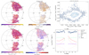 |
Fig. 2. Fit results of the combined (β ≡ 0.5) density model to the O VIII eRASS1 intensity data. The four maps on the left-hand side show the eRASS1 selected data (top left) and the best-fit model intensities (bottom left; including all the background and foreground components and using the same color scale as the data); the logarithm of the ratio data/model in the range 10−0.3 ≃ 0.5 to 100.3 ≃ 2 (top center); and the residuals (data-model)/error (bottom center). The plots on the right show the data intensities against the predicted best-fit model intensities (top right) and an example latitudinal profile extracted along the l = 240 deg line (bottom right) highlighting the contribution of the different modeled components. |
The presence of a spherical component allows for accounting of the column densities derived from O VII absorption line studies, which are otherwise systematically underestimated, as shown by Fig. 3. The absorption column density of the warm-hot plasma is proportional to the plasma density ∝nL rather than ∝n2L. This makes the length L, and thus the plasma scale length, more relevant with respect to the density in absorption rather than emission data. In fact, a model including only a disk-like component systematically underestimates the observed equivalent widths of z = 0 O VII lines detected in the spectra of background quasars (Gupta et al. 2012; Kaaret et al. 2020).
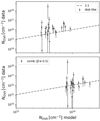 |
Fig. 3. Absorption column density data of O VII (Miller & Bregman 2013) versus model. The disk-like model systematically underestimates the absorption column densities. The inclusion of a spherical β model allowed us to account for them. A combination of the two model geometries thus explains both absorption and emission data. |
On the basis of the χ2 statistic, all the realizations of the combined models with different β are similarly good, with a very small preference (Δχ2 ≃ −357 over ∼31 416 d.o.f.) for the value β = 0.5 with the inclusion of an SWCX model. Given this degeneracy, in the following sections we consider the combined (β ≡ 0.5) model as a reference for comparison with other results presented in the literature. Although we stress that an actual fit of the halo β parameter is currently prevented by X-ray intensity data, β ≡ 0.5 is considered with respect to other solutions also derived on the basis of theoretical arguments4. Nevertheless, we take into account the systematic uncertainty introduced by the choice of β on other derived quantities (e.g., MW baryonic mass Mb and fraction fb, see Sect. 5).
4.2. Oblate disk-like model
From the results of the combined (β ≡ 0.5) model, it follows that the majority of the CGM X-ray emission is produced by the disk-like component (see the lower-right panel in Fig. 2). It is thus instructive to see how the fit is affected when using only this disk-like component. This case has the advantage of simplifying the model description, though at the expense of not accounting for the observed O VII absorption.
When looking at the fit residuals (Fig. 4) and χ2 statistic (Table 1), the disk-like model overall does not perform significantly worse than the combined (β ≡ 0.5) model and provides a similar scale length Rh = 8.0 ± 0.3 kpc. However, the scale height zh significantly increases to zh = 3.3 ± 0.1 kpc. This is explained by the portion of the emission previously attributed to the halo (increasingly important at high |b| and absent in the disk-like model) having to be accounted for in the disk-like component alone, which in turn increases the scale height (cf. the profiles in Figs. 2 and 4). Based only on the eROSITA data, we cannot disfavor a scale height zh = 3.3 kpc with respect to 1.1 kpc. However, this can be done by comparing the expected amount of O VII absorption accounted for by the different models. As pointed out above, the disk-like model alone systematically underestimates O VII absorption data.
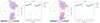 |
Fig. 4. Results of the disk-like (left) and spherical β (right) density model fits to the O VIII eRASS1 intensity data. All the plot details are the same as in Fig. 2. |
4.3. Spherical β model
For completeness, we also tested our data with a fit of a spherical β model alone. Our data selection leaves out most directions at l > 270 deg. This severely reduces the constraining power related to the combination of central density n0 and scale r0 in a spherically symmetric geometry of the plasma. Without the lines of sight toward the Galactic center, these two parameters are in fact highly degenerate with each other. We thus fit the spherical β model using its r ≫ 1 approximation presented in Eq. (5). Looking at the right panels in Fig. 4, the β model (χ2/d.o.f. = 1.89) can account for the sky average count rate, as the ratio data/model (upper central panel) lays within the 0.5−2 range across most of the sky. However, from the data we observed a systematic increase of the count rates with a decreasing |b| at all longitudes that cannot be accounted for by a spherical geometry. The same trend was made more evident when looking at the residual (data-model)/err map (Fig. 4). This evidence alone suggests the presence of an oblate disk-like component other than the INST (flat) and CXB (increasing with |b|) as a significant component of the X-ray intensity from the MW (as independently suggested by Yao et al. 2009; Li et al. 2017; Nakashima et al. 2018; Kaaret et al. 2020 using Chandra, XMM-Newton, Suzaku, and HaloSat data, respectively). Our analysis of the eRASS1 data provides an unambiguous signal for this oblate component, which is detected with a very high significance. We discuss the possible nature of this emission in Sect. 5.
The very flat best-fit slope of the density distribution of the spherical halo β = 0.23 is likely biased toward lower values in order to accommodate lower rates at high latitudes and higher rates at lower latitudes together. Such a flat slope would also result in a nonphysical diverging emission for r → ∞.
Previous studies focusing on only very high latitude regions have found steeper slopes consistent with β = 0.5 (Li & Bregman 2017). By fixing β ≡ 0.5, the fit worsens (χ2/d.o.f. = 1.97, not shown), showing even larger residuals at low latitudes, and the central normalization increases by an order of magnitude, probably to maintain a similar average density (i.e., intensity) value across the volume. Overall, the spherical β model alone reproduces the average intensity of the sky but poorly adapts to the morphology of the eRASS1 O VIII band image.
4.4. Systematic uncertainties
We tested the combined models for different choices of β, namely, β ≡ 0.3, 0.5, 0.7. The best-fit parameters of the combined models still show some degeneracy with β. The central density of the β component C and the scale length of the disk-like component Rh increase with β, while the central density of the disk-like component n0 decreases with β. The scale height of the disk does not show a clear trend and is found in the range zh ∼ 1 − 3 kpc.
We found a minor but not significant preference for the β ≡ 0.5 realization of the combined model including the SWCX based on the χ2 statistic. In the β ≡ 0.3 combined fit, the β-model is suppressed, while the disk-like component dominates the model intensity, showing the same parameters as in the disk-like CGM model. This is probably due to the fact that a β ≡ 0.3 profile looks flatter across the sky than for higher β. This brings the dominating trend with |b| in the data to be mainly fitted by means of the other components (i.e., the disk-like), which in turn leaves only a little residual intensity available for the fit of the β model. The β ≡ 0.7 fit instead shows a large central normalization C due to the mentioned degeneracy between the various parameters (see Fig. D.2). The scale length Rh and height zh of the disk-like component also increase, due to the density left unaccounted for by the steeper roll-off (β = 0.7 > 0.5).
We tested three additional models (combined+swcx, combined+20%instr, and combined+highϵ) in order to assess the systematic errors respectively introduced by the introduction of a (minor) SWCX emission component, a potential systematic underestimation of the instrumental noise or CXB component at soft energies, and the choice of temperature of the plasma component and the spectral modeling of the soft X-ray emission. In the combined+swcx model, we introduced a characterization of the SWCX component in the O VIII band of the eRASS1 data (Dennerl et al., in prep.; see also Appendix C). We compared the estimated CGM flux with an XMM-Newton measurement obtained after subtraction of SWCX (Koutroumpa et al. 2007). We consider the latter measurement to be among the most detailed measurements of the MW CGM component, as it relies on a careful model of the SW Parker spiral in space and time as well as on high spectral resolution data obtained by the Reflection Grating Spectrometer onboard XMM. For the only available field in the western sky (i.e., the Marano field: l, b = 269.8, − 51.7 deg), the authors report FOVIII, cgm = 1.41 ± 0.49 L.U. From the analysis of the eRASS1 data with the inclusion of our SWCX model, we found a consistent value of  L.U.
L.U.
After introducing the SWCX component into the modeling of the eFEDS spectrum, the temperature of the CGM component increases from kT = 0.15 keV to kT = 0.17 keV (Ponti et al. 2023). We introduced this change accordingly in the combined+swcx model. We estimated differences of −30, +96, −37, −18% respectively for the C, n0, Rh, and zh parameters of the combined+swcx with respect to the combined (β ≡ 0.5) model. The morphological parameters Rh and zh change mostly due to a nonuniform morphology of the (faint) SWCX component. The shrunken scale length Rh then requires the normalizations C and n0 in order to adapt while accounting in general for the +16% increase in temperature kT (and in turn emissivity).
We confirmed similar trends when looking at the systematic introduced by a potential underestimation of either the INST or the CXB component (or the sum of them; combined+20%instr model). Given that these are very bright components in the O VIII band, we wanted to assess the sensitivity of our results with respect to the modeling of these components. We estimated −6, +19, −26, and −18% differences with respect to the combined (β ≡ 0.5) model. The systematic shift is comparable or smaller on all parameters with respect to the one caused by the inclusion of the SWCX component.
In addition, we tested different temperature kT = 0.225 keV and metallicity Z = 0.3 Z⊙ assumptions on the CGM modeling through the combined+highϵ model. In practice, both the temperature and metallicity only act on the emissivity ϵ(T, Z) of the APEC model, which in turn does not affect the fit of the morphological parameters (Rh and zh do not change with respect to the combined (β ≡ 0.5) model). Both normalization factors C and n0 decrease by ∼70%, compensating for the boosted emissivity ϵOVIII due to the higher temperature and oxygen abundance.
The strong dependence of the normalization parameters on temperature and emissivity (both fixed quantities in our model) on the one hand stresses the large uncertainty affecting the baryon budget encompassed by the spherical halo component even more (see Sect. 5.3), while on the other hand it also strengthens the evidence for the presence of a disk-like component, as the best fit values of Rh and zh rely mostly on the morphology of the data rather than on assumptions regarding the physical properties of the plasma. This also remains true for a scenario in which (part of) the plasma is at a different temperature than the one assumed in this work, or out of equilibrium. Nearby emission can, in principle, be produced as well by outflowing hot gas out of thermal equilibrium. However, (a lack of) equilibrium mainly affects gas emissivity, which in turn plays a role only in the determination of the density normalization rather than on the fitted geometry. The Rh and zh parameters are thus relatively solid against the assumption of a collisionally ionized plasma in thermal equilibrium, unless the distribution of the temperature and equilibrium phase changes significantly across the sky.
5. Discussion
In this section, we explore some further implications of our fit results. This includes the effects produced by our assumptions.
5.1. The disk-like component is brighter than the spherical halo
The fraction of the observed X-ray intensity coming from the extended hot halo component has so far been left undetermined, or only partially accounted for, due to the limited X-ray intensity data structures that were available before the advent of eROSITA. By simulating and reprojecting the expected emission from the components of the combined (β ≡ 0.5) model (the overall model intensity is shown in the lower-left panel of Fig. 2), we show in Fig. 5 the ratio between the projected O VIII intensity of the halo (β) and the disk-like component in the combined (β ≡ 0.5) model. The ratio is mostly dependent on Galactic latitude |b|, with a slight dependence over longitude l as well. The ratio is less than one in all directions, reaching values as low as 10% at |b|∼20 deg. The ratio confirms that the oblate disk-like component provides most of the counts attributed to the CGM in the O VIII band in all directions. Only at high |b|> 80 deg do the spherical and oblate components result in about the same emission. Previous analyses of high-latitude soft-X background data (Kaaret et al. 2020) have already pointed out the improvement in the fit that results from including a spherical and a disk-like component rather than a single one. Our result confirms that this procedure is necessary, as the model components generally hold comparable levels of emission, whereas the spherical component only provides a minor contribution at low latitudes.
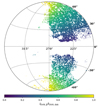 |
Fig. 5. Intensity ratio between the spherical β halo and disk-like components in the O VIII band for the combined (β ≡ 0.5) model. The disk-like component is brighter everywhere. The two components are about equal only at the Galactic poles. |
We stress that the situation described by Fig. 5, as most of the results presented in this work, remains true regardless of the nature of the disk-like component. In fact, a population of unresolved sources with a (thick) disk-like geometry as well as a truly diffuse plasma embracing the stellar disk, or even emission arising from the ISM, can all be explained by a disk-like geometry component of the emission.
5.2. Most of the plasma emission is produced within a few kiloparsecs
From the combined (β ≡ 0.5) model, we predicted where most of the observed emission is produced. In Fig. 6, we plot the cumulative surface brightness of the spherical β and disk-like components of the combined (β ≡ 0.5) model as a function of the distance from the Sun s. The height of a line at a given distance s tells us in practice how much emission has been produced within that distance by that component of the model. Given the general nonspherical symmetry of the projected emission, we computed the profiles for (l, b) = (270, 40) deg. A line of sight at b = 80 deg is also shown for the combined (β ≡ 0.5) model for comparison (dot-dashed line). The hatched areas encompass the 10 − 90 percentile of the surface brightness distribution of each component and model. We plotted different models in order to assess the systematic errors.
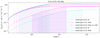 |
Fig. 6. Cumulative surface brightness as a function of the distance from the Sun s. For each model, the dotted and dashed lines respectively show the spherical and disk-like components. The hatched areas encompass the 10 − 90 percentile of the surface brightness distribution. |
We first highlight how the choice of assumed temperature kT and metallicity Z affects the density normalizations but leave the emission profile unchanged in practice. In fact, for simplicity we do not show the combined+highϵ model curves in Fig. 6, as they would entirely coincide with the magenta lines. We have already pointed out this feature of the models. Differently, a change in β affects the emission profile, mainly distributing the emission in the spherical component over a broader (narrower) and larger (closer) range of distances for lower (higher) β while only slightly affecting the disk-like component. In general, the disk-like component always cumulatively produces a larger amount of emission and has a faster increase with s. Most of the emission is in fact produced between 0.2 and 5 kpc from the Sun (median ∼1 kpc), including all systematic uncertainties.
We note that the lower bound of this range is potentially in conflict with our assumption of the absorption happening in front of the X-ray emission with respect to the Sun, as clouds at latitudes |b|∼20 deg above the Galactic plane are found up to distances of 1 kpc (Lallement et al. 2019). At the lower latitudes, breaking the assumption of a single foreground layer of colder gas may explain (part of) the positive residual that is still visible (e.g., Figs. 2 and 4). Loosening the assumption would unfortunately require the introduction of additional degrees of freedom, greatly increasing the degeneracy between them. Although we chose not to increase the complexity of our analysis, we point out that only a minor part of the emission in our closest proximity (0.2−0.3 kpc) may be strongly affected by co-spatial absorption, as farther clouds at |b|> 20 deg only provide a minor contribution to the column density (Lallement et al. 2019).
5.3. The spherical halo holds most of the mass, but its precise budget remains highly uncertain
Given our density models and their components, we integrated over the volume and obtained the mass profiles shown in Fig. 7. We note that this time, we integrated and plotted the profile with respect to the distance from the Galactic center rather than from the position of the Sun. Although the disk-like component produces most of the emission, as we have seen above, the component holding most of the mass is the spherical β model. This is due to the slower roll-off of the profile with respect to the exponential of the disk. The density (and pressure) ratio between the spherical halo and the oblate components increases with the distance from the Galactic center r. At large radii, the volume becomes very large V ∝ r3, thus collecting most of the mass. The mass profile becomes steeper for lower (i.e., flatter) β profiles, as the density decreases more slowly for lower β. Contrary to the surface brightness profiles, in this case the assumptions on temperature kT and metallicity Z of the plasma contribute largely to the systematic offset of the mass profile, as they mainly affect the normalization C and in turn the overall mass. At about the virial radius Rvir ≃ 250 kpc, depending on the choice of β, kT, and Z, the overall mass of the hot gas ranges between some ×109 to some 1010 M⊙. Thus, the fraction of baryons present in the MW potential well cannot be compared to the cosmic fraction fb to almost an order of magnitude of uncertainty. Provided that it makes sense to expect a baryon fraction fb within the virial radius of one galaxy to be similar to the cosmic value (Lochhaas et al. 2021) and given the very large systematic uncertainty affecting the hot gas mass models, we could only qualitatively infer some fraction of the baryons that were seemingly missing from the MW expected budget.
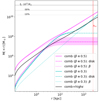 |
Fig. 7. Cumulative mass of the hot gas as a function of the distance from the Galactic center r. For the combined (β ≡ 0.5) model, the solid and dashed lines respectively show the spherical and disk-like components. The horizontal gray lines show 10%, 30%, and 100% of fb × 1012 M⊙, where fb ≡ Σb/Σm = 0.071 is the cosmic baryon fraction. |
5.4. The disk-like emission is consistent with the projected mass distribution of the stellar disk
In this work, we confirmed the existence of a component of the soft X-ray background emission holding a disk-like geometry (to the zeroth order). A straightforward question arises as to whether this component can potentially be linked to a population of sources in the MW stellar disk or if it instead truly arises from a diffuse plasma component. Provided that a diffuse disk-like plasma component would be related to stellar populations anyway, simply through the shared MW gravitational potential and the origin of the heated plasma, the question can be recast as whether the oblate component is the emission of an unresolved X-ray emitting stellar population or if it is of a diffuse plasma. In fact, as anticipated above, the geometry of this component alone does not allow for the exclusion of either of the hypotheses.
The hypothesis of an unresolved M dwarf stellar population producing part of the soft X-ray flux has already been suggested as an explanation for the ∼0.7 keV component, but it is considered unlikely due to the smaller scale height attributed to the M dwarf population (Masui et al. 2009; Yoshino et al. 2009). However, the scale height of the M dwarfs may be larger than previously assumed, as new models of the mass distribution of the MW disk seem to suggest (McMillan 2017). In addition, M dwarfs may have an emission component at temperatures as low as kT = 0.1 − 0.2 keV (Magaudda et al. 2022), thus also producing O VIII. We computed the MW mass surface density profile following (McMillan 2017) and projected it at the Sun position5. The result is shown in the right panel of Fig. 8, next to the O VIII emission measure (EM) computed for the combined (β ≡ 0.5) model (left panel). The profiles show a remarkably similar morphology. This is also highlighted by the scatter plot in Fig. 9, showing the two quantities one versus the other. We find it very interesting how despite showing different and completely independent quantities, each derived by completely independent data, the points generally follow the 1:1 relation, albeit with some scatter. At high EM values (and high ΣM; i.e., close to the Galactic plane), the relation shows some deviation, suggesting a slightly different trend. Indeed, the trend is mainly determined by the scale height of the combined (β ≡ 0.5) model (zh = 1.1 ± 0.1 kpc) with respect to the value used to compute the mass profile (zh = 0.9 kpc; McMillan 2017). Considering the systematic uncertainty in our result, the profiles are consistent with each other.
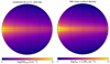 |
Fig. 8. Comparison between the projected morphologies of the combined (β ≡ 0.5) model EM (left panel) and the MW mass surface density (right panel) profiles. The mass surface density ΣM has been arbitrarily renormalized to show the same range of (log) values [17, 19]. |
We note that the normalizations in Fig. 9 are clearly not directly comparable, as they originate from different quantities. Furthermore, the median of the compared models is set equal by definition. The shift c between the EMOVIII and ΣM normalizations may or may not contain information on the luminosity of the stellar population potentially contributing to the X-ray background emission.
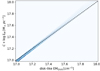 |
Fig. 9. Scatter plot of the quantities shown in Fig. 8. The dashed black line shows the 1:1 relation between them. |
Although the geometrical similarity between the X-ray emission of the disk-like component and the projected mass profile looks interesting, we stress that the mass and the combined (β ≡ 0.5) models compared in Figs. 8 and 9 are the result of a particular choice among the possible models that we showed as still being affected by some systematic uncertainties. In addition, using a geometry-independent approach, Nakashima et al. (2018) estimated the M dwarf unresolved emission from the faint end of their log N − log S and found it to account for less than 20% of the CGM flux in the soft X-ray. The EM and ΣM may thus eventually differ significantly.
The EM of the warm-hot CGM component has also been reported to scale linearly with the EM of the hot component as EMwarm − hot ∼ 10.8 × EMhot across high (absolute) latitude regions, after their detection by HaloSat (Bluem et al. 2022). The authors interpret the EM relation disfavoring the stellar coronae as being responsible for the emission of the hot phase. Their interpretation is based on the assumption that the warm-hot phase is produced by diffuse plasma. By giving up this assumption, the emission of both the warm-hot and the hot phases may be contributed by stellar coronae emission (in part or entirely). However, both the warm-hot and hot phases have been detected through absorption lines (Das et al. 2019a,b). The detected column densities cannot be explained by the small cross section offered by the stellar coronae, while they are easier to accommodate when assuming a truly diffuse nature of the plasma phases. Though the absorption by the warm-hot component could be accounted for by the spherical halo, the hot phase associated with the disk-like component seems to rule out the unresolved population scenario as its main cause. Our point here is that the potential connection between the soft X-ray emission and an unresolved stellar population, while being disfavored by different probes, is not rejected by our simple comparison. In the future, a dedicated and more quantitative investigation of the contribution of stellar coronae to the soft X-ray emission may be worth pursuing in light of the new mass models for the MW and the amount and quality of the eROSITA data.
However, as already pointed out, the same evidence of a similar scale height between the X-ray disk-like component and the MW mass distribution can be explained by an X-ray emitting gas whose dynamic is governed by the same gravitational potential followed by the stellar thick disk, producing similar scale heights. In this picture, the hot atmosphere is also expected to be stationary up to a first approximation, as a single episode of energy injection (e.g., an outflow from an active star-forming region) is not necessarily expected to correlate with the thick disk height. In the next section, we attempt to assess if such a hot gaseous disk-like component can be supported by the current stellar activity in the MW disk.
5.5. The local star formation rate can sustain the disk-like component
In this section, we investigate the thermal luminosity implied by the emitting gas and how it compares with the luminosity implied by star formation (i.e., supernovae explosions). In Sect. 5.2, we derived that most of the observed emission comes from within a few kiloparsecs from the Sun. We thus computed the X-ray luminosity in the solar neighborhood. We considered a cylinder of radius ΔR = 3 kpc centered on the Sun position and extending for Δz = 3 kpc above and below the MW midplane. The mean density value weighted for the profile of the disk-like component within the cylinder is ⟨n⟩=(3.2 ± 2)×10−3 cm−3. Under the assumption that all the emission is produced by diffuse gas of thermal energy kT = 0.15 keV, its soft X-ray (0.2−2 keV) luminosity is LX = ϵ0.2 − 2 keV ⋅ Vcyl ⋅ ⟨n⟩2 ≃ 6.4 × 1039 erg s−1, where ϵ0.2 − 2 keV(kT = 0.15 keV, Z = 0.1 Z⊙) = 1.16 × 10⁻¹⁵ erg cm3 s−1 is the soft X-ray emissivity, while the corresponding total thermal energy is then Eth = ⟨n⟩VkT = (1.3 ± 0.7)×1054 erg.
We also assessed whether the luminosity LX can be supported by heating from supernova explosions in the solar neighborhood or not. The star formation rate (SFR) in the solar neighborhood has been found to reach a uniform density of ≃(2.2 ± 0.8)×10−3 M⊙ yr−1 kpc−2 (Spilker et al. 2021), thus providing SFR ≃ (6.2 ± 2.2)×10−2 M⊙ yr−1 within the closest 3 kpc. Given an SFR, the supernova explosion rate can be estimated through the conversion factor α = 8.8 × 10⁻³ SN  obtained for MW-like galaxies (Horiuchi et al. 2011; Adams et al. 2013). The rate of supernovae in the solar neighborhood (< 3 kpc) is thus ṄSN = α · SFR = (5.4 ± 2.0) × 10−4 yr−1 (i.e., one supernova every ∼1000 − 3000 years). Assuming a supernova energy of ESN = 1051 erg spent to heat the surrounding gas, the supernova luminosity is then LSN = ESN · ṄSN = (1.7 ± 0.6) × 1040 erg s−1. The supernova luminosity LSN is thus comparable to the X-ray plasma luminosity LX, implying that the disk-like component may be powered (in part or entirely) by the current supernova rate in the stellar disk.
5.6. Pressure balance between the disk-like component and high velocity clouds
We constructed the pressure profile of the disk-like warm-hot component as a function of height |z| from the MW midplane at the Sun position. This pressure can be compared with the one derived for high-velocity clouds (HVCs) at moderate and high Galactic latitude. The HVCs show pressure gradients between the core and the outer layers and require an external pressure support in order not to dissolve in a too short timescale (Wakker & van Woerden 1997). In this section, we investigate if the warm-hot disk-like component can provide such a pressure support and if equilibrium with the HVC pressure is reached.
We plot the HVC pressures in Fig. 10 as a function of their height from the MW midplane. Between the few HVCs with available estimates of their pressure, we selected the ones at moderate and/or high Galactic latitudes (|b|> 40 deg). The HVC pressure measurements in fact are degenerate with respect to the (unknown) cloud distances d from the Sun, following P ∝ d−1 (Wakker & Schwarz 1991). For high-latitude clouds, the assumption d ∼ z introduces a smaller bias in the vertical pressure profile Pz than for clouds at lower latitudes. We also computed the pressure profile derived for the warm-hot disk-like component of our best-fit model. The model was computed at the Sun position, following n⊙e−|z|/zh.
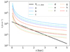 |
Fig. 10. Vertical pressure profile Pz, ⊙, disk computed at the Sun position. The dashed lines show the pressure measurements of HVCs available in the literature: from Wakker & Schwarz (1991) MI.1 (a, [l, b] = [165, 70] deg), AIV.1 and AIV.2 (b and c, respectively; [l, b] = [153, 40] deg) and from Fox et al. (2005) along the line of sight of HE 0226−4110 ([l, b] = [354, −66] deg) HVC.1 (d), HVC.2 (e), HVC.3 (f), HVC.4 (g) and along the line of sight of PG 0953+414 ([l, b] = [180, +52] deg) HVC.1 (h), and HVC.2 (i). The pressure of the HVCs is degenerate with distance, following ∝z−1. |
We found that the pressure of the disk-like gas component is in the same ballpark as the ambient pressure required for HVCs, with moderate scatter. We note that the detailed picture for each cloud may be dependent on other sources of (nonthermal) pressure support within the clouds (e.g., turbulence, magnetic, cosmic rays) that may produce the scatter in the profiles. The HVCs with the highest pressure may even be found at distances greater than 5 kpc, where the spherical halo pressure component starts to dominate over the disk. However, the general order of magnitude agreement in the disk suggests a physical link between the hot gas pressure and the HVC pressure, which would not have reason to match otherwise. In addition, by assuming our model, the distance to the HVCs can be roughly derived at a few kiloparsecs from the Sun, broadly agreeing with the recent constraints put on other HVCs of similar properties (Lehner et al. 2022).
5.7. Results in context
Analyses of the O VIII line intensities for the study of the diffuse Galactic background have been already conducted using different instruments. In general, the various instruments (e.g., XMM-Newton, Suzaku, HaloSat, eROSITA) have different fields of view and spectral resolution; reach different levels of spatial resolution; and cover a different total sky area. In addition, and potentially based on the information retrieved by a given instrument, different authors may adopt different assumptions regarding the physical properties of the hot CGM of the MW (e.g., kT, Z) when required. Despite these differences, a consistent picture arises from the experiments.
In Fig. 11, we show the parameters derived by similar studies for the density profile of the disk-like component. We focus on the disk-like component, as it produces most of the emission attributed to the CGM X-ray emission. We first note that thanks to the sky coverage and spatial resolution of eROSITA, the statistical uncertainties are the smallest to date. Despite this, the physical assumptions necessarily introduce systematic biases in the results, as evidenced by the significant shift of the best-fit parameters for the different models summarized in Table 1 (empty magenta stars) with respect to the combined (β ≡ 0.5) model (filled magenta star). Compared with the other works, we find an overall agreement on zh ∼ 1 − 3 kpc, with some preference toward the lower end of the range. The agreement likely comes from the fact that no physical assumption (i.e., kT, Z) is required to fit these parameters. Again, we note that the lower bound of a scale height of 1−3 kpc is not too far from the one estimated for the thick-disk component of the MW of zthick = 0.9 kpc (McMillan 2017), as discussed above. If the source of the disk-like emission is a truly diffuse plasma, the normalization of the profile n0 really indicates a density value. Although n0 shows inconsistency between experiments when only the statistical uncertainties are taken into account, we note that assumptions on temperature and metal abundances shift n0 across the parameter space. Considering that our combined (β ≡ 0.5) model assumes kT = 0.15 keV and Z = 0.1 Z⊙, n0 is consistent with the approximately two to four times lower values found using HaloSat (kT ≃ 0.225, Z ≡ 0.3 Z⊙; Kaaret et al. 2020) and Suzaku (kT ≃ 0.28, Z ≡ Z⊙; Nakashima et al. 2018), within uncertainties, as shown by our combined+highϵ model holding similar assumptions. The large statistical uncertainty on the value estimated using XMM (Li & Bregman 2017) relates to the small sky coverage of the experiment. Furthermore, a minor but additional scatter across different experiments possibly relates to the different treatment of the background and foreground components other than the hot CGM of the MW.
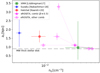 |
Fig. 11. Scale height zh versus n0 derived by different works, as labeled. Error bars only provide statistical uncertainties quoted in the references. |
Using a conservative approach, n0 ≃ 1 − 6 × 10⁻² cm−3 reasonably encompasses the actual value, although we note that, in a sense, n0 still has a more geometrical meaning rather than a physical one for at least two different reasons: (i) our experiments and similar ones are currently only able to probe the CGM using average profile models, while the details at a precise location in space are expected to certainly deviate (within some scatter) from the average picture; (ii) as n0 is the extrapolation of the density profile for (R, z)≪(Rh, zh), there may be no place at all that holds n = n0, as the physics at the Galactic center largely deviate from those assumed in these works.
In Fig. 12, we computed the column density of O VIII emitting gas as seen by an observer far away from the MW and who computes NOVIII as a function of the projected distance from the Galactic center. The different colored solid lines in Fig. 12 show the profiles for our combined (β ≡ 0.5) model (magenta) and some of the other profiles summarized in Table 1, as labeled. In particular, we show the combined (β ≡ 0.3) and combined+highϵ in order to investigate how β, kT, and Z affect NO VIII. In addition, we compared the NO VIII profiles with predictions from the HESTIA simulations of the MW in the Local Group for different initial conditions (please refer to Damle et al. 2022, for details). All of our models are consistent with the HESTIA profiles within the first ∼100 kpc. At larger distances, they seem to overpredict the column density of some of the HESTIA realizations, while they become inconsistent at Rproj > 500 kpc, with the main difference induced by the choice of β. These distances however correspond to ∼2 Rvir, where our assumptions on the physics may be broken by galaxy-galaxy interactions within the Local Group. Although this comparison does not allow us to rule out or to prefer one the models, we find a general agreement between our results and the HESTIA predictions.
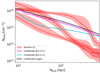 |
Fig. 12. Column density of O VIII versus projected distance Rproj for different models (see Table 1) compared with MW profiles extracted from the HESTIA simulations of the Local Group (Damle et al. 2022). |
Comparat et al. (2022) and Chadayammuri et al. (2022) computed the average eROSITA X-ray (0.5−2.0 keV) surface brightness profile of different populations of star-forming galaxies by stacking cross-matched samples extracted from the eFEDS field. We show a comparison of their results with ours in Fig. 13. We show the same models as in Fig. 12, with the exception of combined+highϵ, as kT and Z only bias the density profile, while leaving the brightness unchanged. The combined+highϵ model and its component would thus overlay everywhere in Fig. 13 to the combined (β ≡ 0.5) model (magenta).
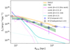 |
Fig. 13. Projected surface brightness profile ΣX as a function of projected distance Rproj from the Galactic center (as seen by an observer far from the MW) in comparison to stacking experiments (Comparat et al. 2022; Chadayammuri et al. 2022) and simulations (taken from Chadayammuri et al. 2022). The dotted and dashed lines show the β halo and disk-like emission components, respectively. The blue triangles indicate upper limits from Comparat et al. (2022). |
The ΣX projected profiles are dominated by the disk-like (β) CGM component below (above) Rproj ∼ 15 − 40 kpc for the combined β ≡ 0.3 − 0.5. For the stacked data profiles, we chose the bins in stellar mass (and star formation) closer to the values inferred for the MW. We advise some caution regarding the comparison with the data for different reasons: (i) In our reprojection of the MW models, we did not include any absorption from the cold ISM. Any realistic galaxy seen from any angle will necessarily be highly absorbed in the central regions in the soft X-ray band. Our profiles at small Rproj are thus mostly upper limits to the actual profile. (ii) The point spread function (PSF) has not been subtracted from the stacking data points, and they are thus consistent with the PSF up to Rproj ∼ 80 kpc (Comparat et al. 2022). (iii) Because of the previous fact and despite the galaxy selection criteria, unresolved contribution from active galactic nuclei may still be present in all the samples, thus biasing the stacking data profile for Rproj < 80 kpc toward high values. (iv) The projection effect with close galaxies (i.e., two-halo term) is considered to be a major contribution at the largest Rproj. For the above reasons, the profiles from the stacking should be considered more as upper limits when compared to our models. All the models considered in Table 1 are well within the upper limits. In this case, both the EAGLE (Crain et al. 2015; Schaye et al. 2015) and TNG (Nelson et al. 2018; Pillepich et al. 2019) simulations (stacked by Chadayammuri et al. 2022) seem to overpredict our combined (β ≡ 0.5) model (magenta).
6. Conclusion
In this work, we analyzed data from the first eROSITA All-Sky Survey of the eROSITA_DE consortium. We exploited a narrowband image (ΔE = 80 eV) produced in an energy range (O VIII) representative of the emission of the warm-hot component attributed to the CGM of the MW at kT = 0.15 − 0.23. We retrieved the CGM emission intensity in the O VIII band by modeling and subtracting the instrumental background and CXB while also taking into account Galactic absorption. We fit the CGM component using three different profiles describing the density of warm-hot gas in the MW: (i) a spherical halo described by a β model, (ii) a disk-like exponential profile characterizing possible stellar feedback or population, and (iii) a linear combination of the previous two.
In accordance with previous studies conducted with different instruments, we find that:
-
(i) a disk-like component virtually accounts for most or all of the observed CGM emission;
-
(ii) the inclusion of a β halo, though only slightly improving the fit of the eRASS1 data, is also necessary to account for O VII absorption column densities observed by XMM as well as the majority of the mass;
-
(iii) the scale height of the disk-like component in the combined model is zh ∼ 1 − 3 kpc, depending on other assumptions (i.e., β, Rh), with a preference toward zh ≃ 1 kpc;
-
(vi) by considering diffuse warm-hot and hot plasma as the source of the disk-like component, most of the emission is produced within ∼5 kpc from the Sun;
-
(iv) the amount of baryons in the hot CGM of the MW is largely unconstrained. In fact, the normalization of the spherical halo C constraining the mass included within Rvir, MW = 250 kpc suffers moderate systematic uncertainties mostly depending on β, kT, and Z;
-
(v) the disk-like profile and scale height is not dissimilar from updated models of MW projected mass profiles (stellar plus gas), suggesting that either some fraction of the emission attributed to the CGM may be contributed by unresolved stellar populations or that the disk-like component is a stationary (i.e., long-lived), gaseous atmosphere following the same gravitational potential as the stellar thick disk;
-
(vi) a truly diffuse nature of the disk-like component can be energetically sustained by star formation (via heating by supernovae explosions), at least locally;
-
(vii) the disk-like component of the warm-hot CGM can provide (part of) the ambient pressure support required by observations of high velocity clouds in the MW.
We also demonstrated the augmented statistical power provided by the quality and amount of the eROSITA data. Our knowledge of the CGM properties is thus now limited by the still necessary physical assumptions on the plasma properties. These assumptions will potentially be loosened by observations of the soft X-ray band with future high-resolution spectrometers (e.g., XRISM, Athena), which will allow individual emission lines to be resolved and in turn kT and Z in the CGM of the MW to be further constrained.
The western half of the sky at 359.9442 > l > 179.9442 deg (great circle over galactic poles and Sgr A*). These are proprietary data of the eROSITA_DE consortium.
G = (f + i)/r, where f, i, and r are respectively the intensities of the forbidden, intercombination and recombination lines (Porquet & Dubau 2000).
In the self-gravitating isothermal sphere (virial) model  is the square of the galaxy-to-gas velocity dispersion ratio (Sarazin 1988; King 1962, although see also Lochhaas et al. 2023).
The complete mass model for the MW must include components such as the nuclear star cluster, the nuclear stellar disk, the Galactic bar, and the Galactic disk. Since our work selects longitudes 180 < l < 300 deg, only the disk component is relevant for our purposes, as all the others only affect the inner |l|< 30 deg.
Acknowledgments
This work is based on data from eROSITA, the soft X-ray instrument aboard SRG, a joint Russian-German science mission supported by the Russian Space Agency (Roskosmos), in the interests of the Russian Academy of Sciences represented by its Space Research Institute (IKI), and the Deutsches Zentrum für Luft- und Raumfahrt (DLR). The SRG spacecraft was built by Lavochkin Association (NPOL) and its subcontractors, and is operated by NPOL with support from the Max Planck Institute for Extraterrestrial Physics (MPE). The development and construction of the eROSITA X-ray instrument was led by MPE, with contributions from the Dr. Karl Remeis Observatory Bamberg & ECAP (FAU Erlangen-Nuernberg), the University of Hamburg Observatory, the Leibniz Institute for Astrophysics Potsdam (AIP), and the Institute for Astronomy and Astrophysics of the University of Tübingen, with the support of DLR and the Max Planck Society. The Argelander Institute for Astronomy of the University of Bonn and the Ludwig Maximilians Universität Munich also participated in the science preparation for eROSITA. The eROSITA data shown here were processed using the eSASS software system developed by the German eROSITA consortium. N.L., G.P. and X.Z. acknowledge financial support from the European Research Council (ERC) under the European Unions Horizon 2020 research and innovation program HotMilk (grant agreement No. [865637]). G.P. also acknowledges support from Bando per il Finanziamento della Ricerca Fondamentale 2022 dell’Istituto Nazionale di Astrofisica (INAF): GO Large program. N.L. thanks Aggeliki Chantzopoulou for her unconditional support. The authors thank Mattia Sormani and Shifra Mandel for fruitful discussion and help.
References
- Adams, S. M., Kochanek, C. S., Beacom, J. F., Vagins, M. R., & Stanek, K. Z. 2013, ApJ, 778, 164 [Google Scholar]
- Anderson, M. E., Gaspari, M., White, S. D. M., Wang, W., & Dai, X. 2015, MNRAS, 449, 3806 [NASA ADS] [CrossRef] [Google Scholar]
- Balucinska-Church, M., & McCammon, D. 1992, ApJ, 400, 699 [Google Scholar]
- Bhattacharyya, S., Das, S., Gupta, A., Mathur, S., & Krongold, Y. 2023, ApJ, 952, 41 [NASA ADS] [CrossRef] [Google Scholar]
- Bluem, J., Kaaret, P., Kuntz, K. D., et al. 2022, ApJ, 936, 72 [NASA ADS] [CrossRef] [Google Scholar]
- Bogdán, Á., Forman, W. R., Vogelsberger, M., et al. 2013, ApJ, 772, 97 [CrossRef] [Google Scholar]
- Bregman, J. N. 1980, ApJ, 236, 577 [NASA ADS] [CrossRef] [Google Scholar]
- Bregman, J. N., & Lloyd-Davies, E. J. 2007, ApJ, 669, 990 [NASA ADS] [CrossRef] [Google Scholar]
- Brunner, H., Liu, T., Lamer, G., et al. 2022, A&A, 661, A1 [NASA ADS] [CrossRef] [EDP Sciences] [Google Scholar]
- Buchner, J. 2021, J. Open Source Softw., 6, 3001 [CrossRef] [Google Scholar]
- Chadayammuri, U., Bogdán, Á., Oppenheimer, B. D., et al. 2022, ApJ, 936, L15 [NASA ADS] [CrossRef] [Google Scholar]
- Comparat, J., Truong, N., Merloni, A., et al. 2022, A&A, 666, A156 [NASA ADS] [CrossRef] [EDP Sciences] [Google Scholar]
- Cox, D. P. 1998, in IAU Colloq. 166: The Local Bubble and Beyond, eds. D. Breitschwerdt, M. J. Freyberg, & J. Truemper, 506, 121 [NASA ADS] [Google Scholar]
- Crain, R. A., Schaye, J., Bower, R. G., et al. 2015, MNRAS, 450, 1937 [NASA ADS] [CrossRef] [Google Scholar]
- Cravens, T. E. 1997, Geophys. Res. Lett., 24, 105 [NASA ADS] [CrossRef] [Google Scholar]
- Damle, M., Sparre, M., Richter, P., et al. 2022, MNRAS, 512, 3717 [CrossRef] [Google Scholar]
- Das, S., Mathur, S., Gupta, A., Nicastro, F., & Krongold, Y. 2019a, ApJ, 887, 257 [NASA ADS] [CrossRef] [Google Scholar]
- Das, S., Mathur, S., Nicastro, F., & Krongold, Y. 2019b, ApJ, 882, L23 [NASA ADS] [CrossRef] [Google Scholar]
- Das, S., Mathur, S., Gupta, A., & Krongold, Y. 2021, ApJ, 918, 83 [NASA ADS] [CrossRef] [Google Scholar]
- Faerman, Y., Sternberg, A., & McKee, C. F. 2017, ApJ, 835, 52 [NASA ADS] [CrossRef] [Google Scholar]
- Forman, W., Jones, C., & Tucker, W. 1985, ApJ, 293, 102 [NASA ADS] [CrossRef] [Google Scholar]
- Fox, A. J., Wakker, B. P., Savage, B. D., et al. 2005, ApJ, 630, 332 [NASA ADS] [CrossRef] [Google Scholar]
- Górski, K. M., Hivon, E., Banday, A. J., et al. 2005, ApJ, 622, 759 [Google Scholar]
- Goulding, A. D., Greene, J. E., Ma, C.-P., et al. 2016, ApJ, 826, 167 [Google Scholar]
- Green, G. 2018, J. Open Source Softw., 3, 695 [NASA ADS] [CrossRef] [Google Scholar]
- Gulick, H., Kaaret, P., Zajczyk, A., et al. 2021, AJ, 161, 57 [NASA ADS] [CrossRef] [Google Scholar]
- Gupta, A., Mathur, S., Krongold, Y., Nicastro, F., & Galeazzi, M. 2012, ApJ, 756, L8 [CrossRef] [Google Scholar]
- Gupta, A., Kingsbury, J., Mathur, S., et al. 2021, ApJ, 909, 164 [NASA ADS] [CrossRef] [Google Scholar]
- Hasinger, G., Burg, R., Giacconi, R., et al. 1993, A&A, 275, 1 [NASA ADS] [Google Scholar]
- Henley, D. B., & Shelton, R. L. 2010, ApJS, 187, 388 [NASA ADS] [CrossRef] [Google Scholar]
- Henley, D. B., & Shelton, R. L. 2012, ApJS, 202, 14 [NASA ADS] [CrossRef] [Google Scholar]
- Henley, D. B., & Shelton, R. L. 2013, ApJ, 773, 92 [NASA ADS] [CrossRef] [Google Scholar]
- HI4PI Collaboration (Ben Bekhti, N., et al.) 2016, A&A, 594, A116 [NASA ADS] [CrossRef] [EDP Sciences] [Google Scholar]
- Hodges-Kluck, E. J., Bregman, J. N., & Li, J.-T. 2018, ApJ, 866, 126 [NASA ADS] [CrossRef] [Google Scholar]
- Horiuchi, S., Beacom, J. F., Kochanek, C. S., et al. 2011, ApJ, 738, 154 [NASA ADS] [CrossRef] [Google Scholar]
- Kaaret, P., Zajczyk, A., LaRocca, D. M., et al. 2019, ApJ, 884, 162 [NASA ADS] [CrossRef] [Google Scholar]
- Kaaret, P., Koutroumpa, D., Kuntz, K. D., et al. 2020, Nat. Astron., 4, 1072 [CrossRef] [Google Scholar]
- Kalberla, P. M. W., & Dedes, L. 2008, A&A, 487, 951 [NASA ADS] [CrossRef] [EDP Sciences] [Google Scholar]
- King, I. 1962, AJ, 67, 471 [Google Scholar]
- Koutroumpa, D., Acero, F., Lallement, R., Ballet, J., & Kharchenko, V. 2007, A&A, 475, 901 [NASA ADS] [CrossRef] [EDP Sciences] [Google Scholar]
- Kuntz, K. D. 2019, A&ARv, 27, 1 [NASA ADS] [CrossRef] [Google Scholar]
- Kuntz, K. D., & Snowden, S. L. 2000, ApJ, 543, 195 [Google Scholar]
- Lallement, R. 2004, A&A, 418, 143 [NASA ADS] [CrossRef] [EDP Sciences] [Google Scholar]
- Lallement, R., Babusiaux, C., Vergely, J. L., et al. 2019, A&A, 625, A135 [NASA ADS] [CrossRef] [EDP Sciences] [Google Scholar]
- Lehner, N., Howk, J. C., Marasco, A., & Fraternali, F. 2022, MNRAS, 513, 3228 [NASA ADS] [CrossRef] [Google Scholar]
- Li, Y., & Bregman, J. 2017, ApJ, 849, 105 [NASA ADS] [CrossRef] [Google Scholar]
- Li, J.-T., Bregman, J. N., Wang, Q. D., et al. 2017, ApJS, 233, 20 [NASA ADS] [CrossRef] [Google Scholar]
- Liu, W., Chiao, M., Collier, M. R., et al. 2017, ApJ, 834, 33 [Google Scholar]
- Lochhaas, C., Tumlinson, J., O’Shea, B. W., et al. 2021, ApJ, 922, 121 [NASA ADS] [CrossRef] [Google Scholar]
- Lochhaas, C., Tumlinson, J., Peeples, M. S., et al. 2023, ApJ, 948, 43 [NASA ADS] [CrossRef] [Google Scholar]
- Lodders, K. 2003, ApJ, 591, 1220 [Google Scholar]
- Magaudda, E., Stelzer, B., Raetz, S., et al. 2022, A&A, 661, A29 [NASA ADS] [CrossRef] [EDP Sciences] [Google Scholar]
- Masui, K., Mitsuda, K., Yamasaki, N. Y., et al. 2009, PASJ, 61, S115 [NASA ADS] [CrossRef] [Google Scholar]
- McCammon, D., Almy, R., Apodaca, E., et al. 2002, ApJ, 576, 188 [NASA ADS] [CrossRef] [Google Scholar]
- McMillan, P. J. 2017, MNRAS, 465, 76 [NASA ADS] [CrossRef] [Google Scholar]
- Merloni, A., Predehl, P., Becker, W., et al. 2012, ArXiv e-prints [arXiv:1209.3114] [Google Scholar]
- Miller, M. J., & Bregman, J. N. 2013, ApJ, 770, 118 [NASA ADS] [CrossRef] [Google Scholar]
- Miller, M. J., & Bregman, J. N. 2015, ApJ, 800, 14 [NASA ADS] [CrossRef] [Google Scholar]
- Nakashima, S., Inoue, Y., Yamasaki, N., et al. 2018, ApJ, 862, 34 [CrossRef] [Google Scholar]
- Navarro, J. F., Frenk, C. S., & White, S. D. M. 1997, ApJ, 490, 493 [Google Scholar]
- Nelson, D., Kauffmann, G., Pillepich, A., et al. 2018, MNRAS, 477, 450 [NASA ADS] [CrossRef] [Google Scholar]
- Nicastro, F., Krongold, Y., Fang, T., et al. 2023, ApJ, 955, L21 [NASA ADS] [CrossRef] [Google Scholar]
- Oppenheimer, B. D., Schaye, J., Crain, R. A., Werk, J. K., & Richings, A. J. 2018, MNRAS, 481, 835 [NASA ADS] [CrossRef] [Google Scholar]
- O’Sullivan, E., Forbes, D. A., & Ponman, T. J. 2001, MNRAS, 328, 461 [NASA ADS] [CrossRef] [Google Scholar]
- Piffaretti, R., Arnaud, M., Pratt, G. W., Pointecouteau, E., & Melin, J. B. 2011, A&A, 534, A109 [NASA ADS] [CrossRef] [EDP Sciences] [Google Scholar]
- Pillepich, A., Nelson, D., Springel, V., et al. 2019, MNRAS, 490, 3196 [Google Scholar]
- Planck Collaboration Int. XLVIII 2016, A&A, 596, A109 [NASA ADS] [CrossRef] [EDP Sciences] [Google Scholar]
- Ponti, G., Zheng, X., Locatelli, N., et al. 2023, A&A, 674, A195 [NASA ADS] [CrossRef] [EDP Sciences] [Google Scholar]
- Porquet, D., & Dubau, J. 2000, A&AS, 143, 495 [NASA ADS] [CrossRef] [EDP Sciences] [Google Scholar]
- Predehl, P., Andritschke, R., Arefiev, V., et al. 2021, A&A, 647, A1 [EDP Sciences] [Google Scholar]
- Qu, Z., & Bregman, J. N. 2019, ApJ, 880, 89 [NASA ADS] [CrossRef] [Google Scholar]
- Revnivtsev, M., Gilfanov, M., Sunyaev, R., Jahoda, K., & Markwardt, C. 2003, A&A, 411, 329 [NASA ADS] [CrossRef] [EDP Sciences] [Google Scholar]
- Sarazin, C. L. 1988, Sky Telesc., 76, 639 [NASA ADS] [Google Scholar]
- Schaye, J., Crain, R. A., Bower, R. G., et al. 2015, MNRAS, 446, 521 [Google Scholar]
- Shapiro, P. R., & Field, G. B. 1976, ApJ, 205, 762 [NASA ADS] [CrossRef] [Google Scholar]
- Smith, R. K., Brickhouse, N. S., Liedahl, D. A., & Raymond, J. C. 2001, ApJ, 556, L91 [Google Scholar]
- Smith, R. K., Bautz, M. W., Edgar, R. J., et al. 2007, PASJ, 59, 141 [Google Scholar]
- Snowden, S. L., & Schmitt, J. H. M. M. 1990, Ap&SS, 171, 207 [NASA ADS] [CrossRef] [Google Scholar]
- Snowden, S. L., Egger, R., Freyberg, M. J., et al. 1997, ApJ, 485, 125 [Google Scholar]
- Snowden, S. L., Collier, M. R., & Kuntz, K. D. 2004, ApJ, 610, 1182 [Google Scholar]
- Spilker, A., Kainulainen, J., & Orkisz, J. 2021, A&A, 653, A63 [NASA ADS] [CrossRef] [EDP Sciences] [Google Scholar]
- Strickland, D. K., Heckman, T. M., Colbert, E. J. M., Hoopes, C. G., & Weaver, K. A. 2004, ApJS, 151, 193 [Google Scholar]
- Sunyaev, R., Arefiev, V., Babyshkin, V., et al. 2021, A&A, 656, A132 [NASA ADS] [CrossRef] [EDP Sciences] [Google Scholar]
- Tüllmann, R., Pietsch, W., Rossa, J., Breitschwerdt, D., & Dettmar, R. J. 2006, A&A, 448, 43 [CrossRef] [EDP Sciences] [Google Scholar]
- Tumlinson, J., Peeples, M. S., & Werk, J. K. 2017, ARA&A, 55, 389 [Google Scholar]
- Wakker, B. P., & Schwarz, U. J. 1991, A&A, 250, 484 [NASA ADS] [Google Scholar]
- Wakker, B. P., & van Woerden, H. 1997, ARA&A, 35, 217 [NASA ADS] [CrossRef] [Google Scholar]
- White, S. D. M., & Rees, M. J. 1978, MNRAS, 183, 341 [Google Scholar]
- Willingale, R., Starling, R. L. C., Beardmore, A. P., Tanvir, N. R., & O’Brien, P. T. 2013, MNRAS, 431, 394 [Google Scholar]
- Yao, Y., Wang, Q. D., Hagihara, T., et al. 2009, ApJ, 690, 143 [NASA ADS] [CrossRef] [Google Scholar]
- Yeung, M. C. H., Freyberg, M. J., Ponti, G., et al. 2023, A&A, 676, A3 [NASA ADS] [CrossRef] [EDP Sciences] [Google Scholar]
- Yoshino, T., Mitsuda, K., Yamasaki, N. Y., et al. 2009, PASJ, 61, 805 [NASA ADS] [Google Scholar]
- Zheng, Y., Peeples, M. S., O’Shea, B. W., et al. 2020, ApJ, 896, 143 [NASA ADS] [CrossRef] [Google Scholar]
- Zheng, X., Ponti, G., Freyberg, M., et al. 2024, A&A, 681, A77 [NASA ADS] [CrossRef] [EDP Sciences] [Google Scholar]
- Zhu, H., Tian, W., Li, A., & Zhang, M. 2017, MNRAS, 471, 3494 [NASA ADS] [CrossRef] [Google Scholar]
- Zonca, A., Singer, L., Lenz, D., et al. 2019, J. Open Source Softw., 4, 1298 [Google Scholar]
Appendix A: X-ray absorption
We assumed the neutral atomic hydrogen column densities NHI from the full sky HI4PI radio survey (HI4PI Collaboration 2016). In general, the content of atomic hydrogen NHI differs from the total content of hydrogen in both atomic and molecular form NH. We computed the total hydrogen column density NH as
 (A.1)
(A.1)
![Mathematical equation: $$ \begin{aligned} N_{\rm H_2}&= 7.2 \times 10^{20} \left[1 - \exp \left(\frac{-N_{\rm HI} E_{\rm B-V}}{3.0 \times 10^{20}}\right)\right]^{1.1}, \end{aligned} $$](/articles/aa/full_html/2024/01/aa47061-23/aa47061-23-eq17.gif) (A.2)
(A.2)
where NH2 is the molecular hydrogen column density in cm−2 and EB − V is the optical reddening caused by dust extinction (Willingale et al. 2013, Eq. 7). The optical reddening has been taken from the Planck Collaboration Int. XLVIII (2016) results, extracted using the dustmaps tool of Green (2018). The computed total hydrogen column density map NH is shown in Fig. A.1. At high absolute Galactic latitudes, the northern hemisphere shows, on average, a larger column density with respect to the southern hemisphere. The total hydrogen column density was also computed through a direct correlation with the optical extinction in the V-band Av as NH = 2.04 × 10²¹Av (Zhu et al. 2017), where Av = RvEB − V with Rv = 3.1 as the total-to-selective extinction ratio. The two methods provide consistent NH values, with the largest discrepancies produced only for large NHI lines of sight, mainly involving very low Galactic latitudes. In fact, we note that at high enough Galactic latitudes, which is where we focus our analysis, the relatively low column densities (NHI < 1021 cm−2) limit the presence of molecular gas not probed by HI surveys and makes the two different NH estimates consistent with each other within a few percent. We assumed the CGM and CXB emission components are located behind all of the absorbing layers, thus accounting for the whole NH value for all lines of sight.
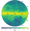 |
Fig. A.1. Total hydrogen column density NH map of the foreground absorption. |
Appendix B: Local hot bubble
The LHB emission becomes increasingly important toward softer energies. This fact is supported by both spectral analysis (Fig. 5 in Ponti et al. 2023) and the morphology of the soft emission, as it highly resembles that of the 1/4 keV ROSAT map thought to be dominated by such a component (Snowden et al. 1997). The latter argument in particular, considering the different background particle environments of eROSITA and ROSAT (Snowden et al. 1997; Predehl et al. 2021), implies the importance of LHB photons with respect to the instrumental particle background in the soft band. A detailed modeling of the LHB emission measure has been provided by Liu et al. (2017), who quantified and removed from the ROSAT data the contribution from the spurious component of the solar wind charge exchange (SWCX) thanks to data collected with a dedicated rocket mission. By assuming thermal ionization equilibrium, the authors provided an emission measure map of the LHB, which was found to be at a remarkably homogeneous temperature of kT = 0.097 ± 0.019 keV across the sky. Although their map derived from the ROSAT data has a lower angular resolution than eROSITA, it is the most robust modeling of the LHB currently available, thanks to the large effective area of ROSAT at very soft energies E ∼ 0.1 keV, where the emission from all the diffuse components become heavily absorbed, except from the LHB. By assuming solar metallicities (Ponti et al. 2023), we then reconstructed the expected LHB emission in all bands, estimating median contributions of 1.20 × 10⁻² ph s−1 deg−2 in the O VIII energy band (i.e., ∼1.3% of the line intensity). The LHB thus only provides a very small fraction of the counts in the O VIII energy band. We attribute a fractional error of 8% to the LHB count rates. This includes possible systematic variations of the LHB temperature estimation Liu et al. (2017).
Appendix C: Solar wind charge exchange
The solar wind is known to be composed of ionized particles that can interact with the neutral ISM. The interaction between the ionized and neutral material through the exchange of electrons was first discovered to produce soft X-rays in the tails of comets (Cravens 1997) and at the interface between the heliosphere and the ISM (Cox 1998). The ISM in fact constantly passes through the heliosphere due to its relative motion with respect to the Sun. Emission lines consistent with charge exchange from the solar wind have been detected by XMM-Newton (Snowden et al. 2004), and their contribution to the 1/4 keV ROSAT map has been found to be important and widespread across the sky (Lallement 2004). Due to the variability and anisotropy of the solar wind, the emission of the SWCX has also been found to be variable in both time and direction (Kuntz 2019). An additional component of the SWCX can be produced at the interaction region between the solar wind and the Earth’s exosphere. However, thanks to the position of eROSITA in L2, this component is expected to be negligible with respect to the one in the heliospheric within our data, while it is potentially relevant for instruments operating at low Earth orbits, such as XMM-Newton or Chandra (Snowden et al. 2004).
The variation of the intensity between the eRASS1 and eRASS2 data is found to be negligible (Ponti et al. 2023; Dennerl et al. in preparation). This implies that if the eRASS1 data are affected by SWCX emission, this component is rather stable over an approximately one-year timescale, at odds with the SWCX properties. In any case, the SWCX intensity has been constrained in the eRASS1 data in the direction of dark clouds (Yeung et al. 2023) to amount to less than 10% of the median observed O VIII intensity. Given the direction of the cloud toward the GC and close to the ecliptic plane, both places where the SWCX is thought to be highest, we can consider this value as an upper limit to the SWCX contribution in the O VIII band. In all the other lines, the SWCX emission is negligible.
Accounting for the SWCX emission in spectral analysis shifts the temperature of the warm-hot component from T = 0.15 keV to 0.17 keV (Ponti et al. 2023). In the combined (β ≡ 0.5) model for the eRASS1 data, we considered the SWCX emission as negligible. However, we investigated what systematic this component may introduce in our results by including it and considering T = 0.17 keV the temperature of the hot phase of the CGM in Sec. 5.
Appendix D: Additional figures
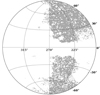 |
Fig. D.1. Data selection mask resulting from a combination of the signal-to-noise ratio < 2σb of the pixels and total hydrogen column density NH < 1.6 × 1021 cm−2. |
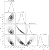 |
Fig. D.2. Corner plot for the parameters of the combined (β ≡ 0.5) model fit using ultranest. |
All Tables
All Figures
|
Fig. 1. eRASS1 O VIII intensity data used in this work. Data are shown using a Zenith Equal Area projection in the Galactic coordinate reference frame and centered at (l, b) = (270, 0) deg throughout this work. We note that the left panel includes the contribution from the eROSITA instrumental background, and the sky flux was processed through the effective area of eROSITA. The right panel shows the same map, but the instrumental background has been subtracted, leaving the signal from the sky (see Eq. (2)). We divided the sky signal by the eROSITA effective area to obtain the surface brightness of the physical sky signal in line units (L.U. = ph s−1 cm−2 sr−1). |
| In the text | |
|
Fig. 2. Fit results of the combined (β ≡ 0.5) density model to the O VIII eRASS1 intensity data. The four maps on the left-hand side show the eRASS1 selected data (top left) and the best-fit model intensities (bottom left; including all the background and foreground components and using the same color scale as the data); the logarithm of the ratio data/model in the range 10−0.3 ≃ 0.5 to 100.3 ≃ 2 (top center); and the residuals (data-model)/error (bottom center). The plots on the right show the data intensities against the predicted best-fit model intensities (top right) and an example latitudinal profile extracted along the l = 240 deg line (bottom right) highlighting the contribution of the different modeled components. |
| In the text | |
|
Fig. 3. Absorption column density data of O VII (Miller & Bregman 2013) versus model. The disk-like model systematically underestimates the absorption column densities. The inclusion of a spherical β model allowed us to account for them. A combination of the two model geometries thus explains both absorption and emission data. |
| In the text | |
|
Fig. 4. Results of the disk-like (left) and spherical β (right) density model fits to the O VIII eRASS1 intensity data. All the plot details are the same as in Fig. 2. |
| In the text | |
|
Fig. 5. Intensity ratio between the spherical β halo and disk-like components in the O VIII band for the combined (β ≡ 0.5) model. The disk-like component is brighter everywhere. The two components are about equal only at the Galactic poles. |
| In the text | |
|
Fig. 6. Cumulative surface brightness as a function of the distance from the Sun s. For each model, the dotted and dashed lines respectively show the spherical and disk-like components. The hatched areas encompass the 10 − 90 percentile of the surface brightness distribution. |
| In the text | |
|
Fig. 7. Cumulative mass of the hot gas as a function of the distance from the Galactic center r. For the combined (β ≡ 0.5) model, the solid and dashed lines respectively show the spherical and disk-like components. The horizontal gray lines show 10%, 30%, and 100% of fb × 1012 M⊙, where fb ≡ Σb/Σm = 0.071 is the cosmic baryon fraction. |
| In the text | |
|
Fig. 8. Comparison between the projected morphologies of the combined (β ≡ 0.5) model EM (left panel) and the MW mass surface density (right panel) profiles. The mass surface density ΣM has been arbitrarily renormalized to show the same range of (log) values [17, 19]. |
| In the text | |
|
Fig. 9. Scatter plot of the quantities shown in Fig. 8. The dashed black line shows the 1:1 relation between them. |
| In the text | |
|
Fig. 10. Vertical pressure profile Pz, ⊙, disk computed at the Sun position. The dashed lines show the pressure measurements of HVCs available in the literature: from Wakker & Schwarz (1991) MI.1 (a, [l, b] = [165, 70] deg), AIV.1 and AIV.2 (b and c, respectively; [l, b] = [153, 40] deg) and from Fox et al. (2005) along the line of sight of HE 0226−4110 ([l, b] = [354, −66] deg) HVC.1 (d), HVC.2 (e), HVC.3 (f), HVC.4 (g) and along the line of sight of PG 0953+414 ([l, b] = [180, +52] deg) HVC.1 (h), and HVC.2 (i). The pressure of the HVCs is degenerate with distance, following ∝z−1. |
| In the text | |
|
Fig. 11. Scale height zh versus n0 derived by different works, as labeled. Error bars only provide statistical uncertainties quoted in the references. |
| In the text | |
|
Fig. 12. Column density of O VIII versus projected distance Rproj for different models (see Table 1) compared with MW profiles extracted from the HESTIA simulations of the Local Group (Damle et al. 2022). |
| In the text | |
|
Fig. 13. Projected surface brightness profile ΣX as a function of projected distance Rproj from the Galactic center (as seen by an observer far from the MW) in comparison to stacking experiments (Comparat et al. 2022; Chadayammuri et al. 2022) and simulations (taken from Chadayammuri et al. 2022). The dotted and dashed lines show the β halo and disk-like emission components, respectively. The blue triangles indicate upper limits from Comparat et al. (2022). |
| In the text | |
|
Fig. A.1. Total hydrogen column density NH map of the foreground absorption. |
| In the text | |
|
Fig. D.1. Data selection mask resulting from a combination of the signal-to-noise ratio < 2σb of the pixels and total hydrogen column density NH < 1.6 × 1021 cm−2. |
| In the text | |
|
Fig. D.2. Corner plot for the parameters of the combined (β ≡ 0.5) model fit using ultranest. |
| In the text | |
Current usage metrics show cumulative count of Article Views (full-text article views including HTML views, PDF and ePub downloads, according to the available data) and Abstracts Views on Vision4Press platform.
Data correspond to usage on the plateform after 2015. The current usage metrics is available 48-96 hours after online publication and is updated daily on week days.
Initial download of the metrics may take a while.