| Issue |
A&A
Volume 689, September 2024
|
|
|---|---|---|
| Article Number | A328 | |
| Number of page(s) | 15 | |
| Section | Galactic structure, stellar clusters and populations | |
| DOI | https://doi.org/10.1051/0004-6361/202449398 | |
| Published online | 24 September 2024 | |
eROSITA narrowband maps at the energies of soft X-ray emission lines
1
Max-Planck-Institut für extraterrestrische Physik, Gießenbachstraße 1, D-85748 Garching bei München, Germany
2
INAF-Osservatorio Astronomico di Brera, Via E. Bianchi 46, I-23807 Merate (LC), Italy
3
Dr. Karl Remeis Observatory, Erlangen Centre for Astroparticle Physics, Friedrich-Alexander-Universität Erlangen-Nürnberg, Sternwartstraße 7, 96049 Bamberg, Germany
Received:
30
January
2024
Accepted:
29
June
2024
Abstract
Hot plasma plays a crucial role in regulating the baryon cycle within the Milky Way, flowing from the energetic sources in the Galactic center and plane, to the corona and the halo. This hot plasma represents an important fraction of the Galactic baryons, plays a key role in galactic outflows and is an important ingredient in galaxy evolution models. Taking advantage of the Spectrum-Roentgen-Gamma (SRG)/eROSITA first all-sky survey (eRASS1), in this work our aim is to provide a panoramic view of the hot circumgalactic medium (CGM) of the Milky Way. Compared to the previous all-sky X-ray survey performed by ROSAT, the improved energy resolution of eROSITA enabled us to map, for the first time, the sky within the narrow energy bands characteristic of soft X-ray emission lines. These lines provide essential information on the physical properties of the hot plasma. Here we present the eROSITA eRASS1 half sky maps in narrow energy bands corresponding to the most prominent soft X-ray lines, O VII and O VIII, which allowed us to constrain the distribution of the hot plasma within and surrounding the Milky Way. We corrected the maps by removing the expected contribution associated with the cosmic X-ray background, the time-variable solar wind charge exchange, and the local hot bubble. We applied corrections to mitigate the effect of absorption, therefore highlighting the emission from the CGM of the Milky Way. We used the line ratio of the oxygen lines as a proxy to constrain the temperature of the warm-hot CGM, and we defined a pseudo-temperature 𝒯 map. The map highlights how different regions are dominated by different thermal components. Toward the outer halo, the temperature distribution of the CGM on angular scales of 2–20 deg is consistent with being constant Δ𝒯/⟨𝒯⟩≤4%, with a marginal detection of Δ𝒯/⟨𝒯⟩ = 2.7%±0.2% (statistical) ±0.6% (systematic) in the southern hemisphere. Instead, significant variations of ∼12% are observed on scales of many tens of degrees when comparing the northern and southern hemispheres. The pseudo-temperature map shows significant variations across the borders of the eROSITA bubbles, suggesting temperature variations, possibly linked to shocks, between the interior of the Galactic outflow and the unperturbed CGM. In particular, a shell characterized by a lower line ratio appears close to the edge of the eROSITA bubbles.
Key words: Galaxy: general / Galaxy: structure / X-rays: diffuse background / X-rays: general
Corresponding author; This email address is being protected from spambots. You need JavaScript enabled to view it. .
© The Authors 2024
 Open Access article, published by EDP Sciences, under the terms of the Creative Commons Attribution License (https://creativecommons.org/licenses/by/4.0), which permits unrestricted use, distribution, and reproduction in any medium, provided the original work is properly cited.
This article is published in open access under the Subscribe to Open model.
Open access funding provided by Max Planck Society.
1. Introduction
As the next generation of all-sky survey experiments in soft X-ray, the extended ROentgen Survey with an Imaging Telescope Array (eROSITA), on board the Russian-German observatory Spectrum-Roentgen-Gamma (Sunyaev et al. 2021), performed the first all-sky survey (eRASS1; Merloni et al. 2024) from December 2019 to June 2020. eRASS1 has an unprecedented sensitivity to the whole sky in the soft X-ray range, thanks to an effective area of ≈1100 cm2 at 1.4 keV, with an energy resolution typical of CCD instruments (≈65 eV at 0.5 keV; Predehl et al. 2021). Hence eROSITA makes it possible to obtain monochromatic images for various emission lines simultaneously from the diffuse emission over the entire sky.
In this paper we present the eRASS1 narrowband maps corresponding to the brightest transitions in the soft X-ray band (i.e., O VII and O VIII), together with the maps ratio, and make these maps (in count rate unit), publicly available online1.
In X-rays, emission lines are vital for understanding the properties of the hot plasma inside the interstellar medium (ISM) and in the circumgalactic medium (CGM), the latter made up of different components, among which the Galactic halo, the Galactic corona, and the Galactic outflow are also included. The halo of the Milky Way is expected to be filled with plasma with temperatures close to its virial temperature2, T ∼ 0.15 − 0.20 keV, and therefore appearing bright in soft X-ray emission lines (Yoshino et al. 2009; Henley et al. 2010; Henley & Shelton 2012; Miller & Bregman 2015). Additionally, Galactic outflows emerging from the center of the Milky Way are expected (and observed) to drive shocks into the ISM and the unperturbed CGM, heating the plasma and inducing bright soft X-ray emission lines (Predehl et al. 2020). Finally, it has been argued that activity in the Galactic plane is expected to sustain a hot Galactic atmosphere (called the Galactic corona), which might also be traced in the soft X-ray band (Das et al. 2019a, 2019b; Ponti et al. 2023a).
Mapping the emission lines from such hot and rarefied plasma is extremely challenging because the corresponding signal is spread over the entire sky and at very low surface brightness. To increase sensitivity to this emission, broadband images can be helpful. The ROSAT all-sky survey allowed us to get a view of the CGM emission in broad energy bands (Snowden et al. 1997; Zheng et al. 2024); however, the O VII and O VIII lines (i.e., the brightest) could not be imaged separately because of the limited energy resolution of ROSAT. With its high sensitivity and band coverage in soft X-ray, eROSITA possesses the specialized capability to image the faint emission in narrower energy bands compared to ROSAT. Here we present the first eROSITA sky maps of the soft X-ray emission lines.
The paper is organized as follows. Section 2 shows the data analysis. Section 3 discusses the soft X-ray emission lines as tracers of hot plasma. Section 4 presents the necessary tools used to retrieve the physical information from the maps. Section 5 discusses the morphology of the line emission maps, their ratio, and the retrieved physical information. Section 6 discusses the observed ratio between emission line maps as a proxy for the plasma temperature. Sections 7 and 8 present the constraints on the temperature of the CGM and the eROSITA bubbles, respectively. We discuss our findings in Sect. 9, and give a summary in Sect. 10.
2. Data
We analyzed the eRASS1 data (Merloni et al. 2024), collected from December 12, 2019, until June 11, 2020. We considered only data from the five telescope modules (TM) of eROSITA cameras equipped with on-chip filter (i.e., TM1, TM2, TM3, TM4, TM6), to avoid any contamination from the effects of light leak (affecting TM 5 and 7, Predehl et al. 2021). We used the same procedures as in Zheng et al. (2024) and analyze the data with the standard eROSITA Science Analysis Software System (eSASS), version 020, developed by the German eROSITA consortium (Brunner et al. 2022). The eROSITA all-sky data are archived in a system of 4700 partially overlapping tiles of  each (Merloni et al. 2024). When required, we re-projected each pixel in each sky-tile, to create a map with an HEALPix3 projection with NSIDE = 512 (Górski et al. 2005; Zonca et al. 2019). The same filtering described in Zheng et al. (2024) has been applied to the counts maps and exposure maps.
The maps display the intensity within the specific energy range in unit of counts per second per square degree [cts s−1 deg−2]. The Zenital Equal Area (ZEA) projection is applied to conserve surface brightness. While the ZEA projection introduces projection distortion, especially toward the borders of the map, we find the distortions less prominent compared to other kinds of possible projections. For display purposes only, several maps presented below were smoothed with an adaptive kernel based on a count rate S/N threshold of 15 to highlight the diffuse emission.
3. Soft X-ray lines as tracers of hot plasma
The electromagnetic spectrum of optically thin and collisionally ionized (hot) plasma consists of continuum emission plus an array of emission lines. For X-ray emitting plasma with temperatures lower than T ∼ 1 keV, the majority of the flux is in fact carried by a large number of weak emission lines. The numerous lines cannot be resolved individually at the CCD energy resolution of eROSITA, forming a pseudo continuum. As an example, the data in the top and bottom panels of Fig. 1 show the eROSITA spectra from two sky regions (eROSITA sky tiles 294147 and 085126, Merloni et al. 2024) characteristics of bright and faint diffuse emission, respectively. The spectra shown in Fig. 1 here are meant to help present the meaning and relations between different emission lines and the spectral components producing them. Both spectra show several peaks associated with the most prominent transitions, which stand out in the eROSITA spectra above the pseudo continuum (Fig. 1).
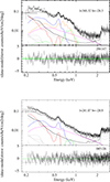 |
Fig. 1. Spectra of the diffuse emission observed by eROSITA within two sky patches of 3° ×3° each. Upper panel: Observed and modeled spectrum of the sky region at |


We focus this work on the two strongest lines observed in the eROSITA spectra of the diffuse emission: O VII and O VIII (see Table 1). We chose the width of the energy bands on the basis of the energy resolution of the pnCCD cameras of eROSITA, as determined on ground (see Table 4 in Predehl et al. 2021). Within these relatively narrow energy ranges, fainter emission lines might contribute to the emission from the pseudo continuum. For this reason, we did not perform any continuum subtraction of the emission lines (e.g., computing the line equivalent width). Instead, we forward modeled the expected emission (assuming the AtombDB library of atomic data and transitions4) in order to compare the data with expectations (see Sect. 4).
Transitions considered in this work and corresponding energy band selected to extract photon lists and to create the corresponding images.
Figure 2 shows an RGB half-sky map of the emission in the O VII, the broad continuum (0.2–2.3 keV) and O VIII bands in red, green and blue, respectively. The RGB image shown in Fig. 2 highlights the emission associated with the hot plasma. All major extended features which are also observed in the broadband maps are seen in Fig. 2 (see Zheng et al. 2024, for a chart map of the principal diffuse structures). In particular, the nearby extended features, such as the Monogem ring (Knies 2022), the Antlia supernova remnant, and the Orion-Eridanus complex (Joubaud et al. 2019) appear as large-scale extended features in a markedly orange color. A greenish and bright patch of X-ray emission is observed around the LMC (Locatelli et al. 2024a). A green-blue color characterizes the interior of the eROSITA bubbles (Predehl et al. 2020) compared with the anti-center direction. Moreover, clear color gradients are observed at the edges of the eROSITA bubbles. The dark regions at small Galactic latitudes b (i.e., along the Galactic plane) in Fig. 2, some of which are as extended as ∼20 deg, are the result of absorption of the soft X-ray emission through the ISM.
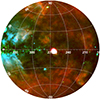 |
Fig. 2. Bright emission lines in eRASS1. The RGB map is composed of the broadband maps at 0.20–0.25 keV (red, Zheng et al. 2024) and 0.2–2.3 keV (green, Zheng et al. 2024), and the narrowband O VIII images (blue, this work). All the maps include the contribution of different components (both celestial and instrumental), and were smoothed with an adaptive kernel set to retrieve a S/N threshold of 15. |
3.1. The dependence of the ion fractions on temperature
Figure 3 shows the expected ion fraction as a function of the plasma temperature for oxygen, as derived from AtombDB under the assumption of an optically thin hot plasma mainly ionized by collisions between atoms. For each element, the ionization fraction is obtained by balancing the net rates of ionization and recombination, which depends on the temperature of the plasma. The vertical dotted gray lines indicate the typical or empirical temperature of some of the components contributing to the soft X-ray diffuse emission. These are: the local hot bubble (LHB), characterized by T ∼ 0.097 keV (Liu et al. 2017); the circumgalactic medium (CGM or halo) of the Milky Way, with T ∼ 0.15 − 0.2 keV (Ponti et al. 2023a); the eROSITA bubbles, which we assume to have T ∼ 0.3 keV (Kataoka et al. 2018; but see also Gupta et al. 2023). Figure 3 shows that plasma with temperatures characteristic of the LHB is dominated by O VII, while the CGM emission has similar contributions from O VII and O VIII, while the O VIII/O VII line ratio becomes insensitive to the presence of plasma at even higher temperatures (i.e., T ≫ 0.3 keV).
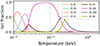 |
Fig. 3. Ionization fraction of oxygen as a function of temperature (from AtomDB, see Smith et al. 2001). The vertical dotted lines in gray show the typical temperatures of LHB (T = 0.097 keV); CGM (T = 0.15 keV); and eROSITA bubbles (assumed to be T = 0.3 keV). |
3.2. Soft X-ray line ratios as temperature diagnostics
As can be seen in Fig. 3, under the assumption of a single emission component in collisional ionization equilibrium, it is possible to measure the temperature of the emitting plasma, given an observed line ratio. In particular, if both ions belong to the same element (e.g., O VII and O VIII), then the line ratio has almost no dependence on the metal abundances of the emitting plasma, therefore becoming a reliable tool to determine the temperature of the hot plasma.
Figure 4 shows the evolution of the O VIII/O VII line ratio as a function of temperature. The line ratio was computed by simulating a collisionally ionized diffuse gas (APEC component in XSPEC) at each temperature. The theoretical spectrum obtained was then convolved with a Gaussian kernel with a full width at half maximum of 74 eV in order to simulate the spectral resolution of eROSITA and compare the theoretical ratio with the data. Finally, the fluxes in each band (see Table 1) were used to produce the expected line ratio as a function of temperature. The lines in the bottom panel of Fig. 4 show that the O VIII/O VII line ratio as observed by eROSITA is an excellent temperature diagnostic for single temperature plasma between T ∼ 0.1 and T ∼ 0.3 keV, while it is insensitive to plasma hotter than T ≥ 0.3 keV. The different lines show line ratios under the assumption that the emitting plasma has a metallicity of 0.1 or 0.3 Solar, as well as holding different ratios between the abundances of the metals (e.g., assuming different abundance sets; Lodders et al. 2009; Anders & Grevesse 1989 and Allen et al. 2019). As expected, in the 0.1–0.3 keV temperature range, where the O VIII and O VII lines are sufficiently bright with respect to the pseudo-continuum, little to no variations of the line ratio are observed with metallicity.
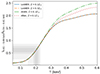 |
Fig. 4. Narrowband intensity ratio as a function of temperature, and absolute and relative metal abundances (as labeled, from AtomDB Smith et al. 2001, and convolved with the eROSITA spectral resolution). The shaded areas encompass 2, 10, 25, 75, 90, and 98% of the distribution of the narrowband intensity ratio analyzed in this work (an image of the data is presented in the top panel of Fig. 9). |
4. Subtraction of non-CGM emission components from the maps
As discussed in Sect. 3.2, from the line ratio maps it is possible to extract important information on the temperature of the CGM, if the emission can be described by a single component of an optically thin plasma in collisional ionization equilibrium. However, the diffuse soft X-ray emission measured by eROSITA has several contributions from various thermal and non-thermal components that need to be removed before we can constrain the temperature of the CGM. Additionally, we expect that the emission from the CGM is, at least in part, absorbed by the interstellar medium, further complicating the interpretation of the line ratio maps. We note that the subtraction of (back-)foreground components is not performed on all the images shown within this paper but is applied to produce and analyze the temperature distribution of some representative sky patches. Below, we provide a description of the corrections we applied to retrieve the temperature map from the data.
4.1. Subtraction of the instrumental background
During the eRASS1 survey, the level of the instrumental background has been frequently monitored, thanks to weekly observations with the filter wheel closed (Yeung et al. 2023). The analysis of these filter wheel closed data shows that the eROSITA instrumental background has been relatively stable in flux and spectrum for the entire duration of eRASS1.
This instrumental background is described by a relatively flat spectrum with various emission lines, as well as detector electronic noise, which is stronger at lower energies and can be represented by a rise in the flux of the instrumental background toward lower energies (solid black line in Fig. 1; see also Yeung et al. 2023). Here, we subtracted the contribution of the instrument background over the entire sky by assuming that it is stable over the duration of the eRASS1 survey.
We stress that the contribution of the background over the narrow O VII band is small, being ∼40 and ∼10 times fainter than the O VII emission in the bright and faint region we denoted in Fig. 1, respectively.
4.2. Removing the contribution from the solar wind charge exchange emission
eRASS1 occurred close to solar minimum when the heliospheric solar wind charge exchange (SWCX) is at its minimum (Kuntz 2019). In addition, eROSITA is located close to the Sun-Earth Lagrangian point L2 (where the effects of the geocoronal SWCX are low). In this context, Ponti et al. (2023a) and Yeung et al. (2023) have reported evidence for a time-variable component affecting the diffuse emission observed by eROSITA. This variable component was attributed to the effects of the heliospheric SWCX. The impact of SWCX is found to be minimal during eRASS1 (Yeung et al. 2023; Ponti et al. 2023a) due to a combination of the aforementioned effects: the telescope position at L2 and eRASS1 happening close to solar minimum. The contribution from time-variable components in the sky (including and setting an upper limit to the SWCX) was computed by first producing background maps reporting the minimum values of O VII and O VIII observed by eROSITA between 2019 and 2022 in every direction in the sky. This is possible thanks to the multiple passages of the telescope’s field of view, according to the survey scanning strategy. The minimum map was then used to detect any variable excess in time. We then subtracted the map representing the time-variable excess from the narrowband maps of Figs. 5 and 6.
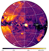 |
Fig. 5. Narrowband map in the energy range of the O VII line as observed by eROSITA during eRASS1 in units of cts s−1 deg−2. An adaptive smoothing kernel using S/N = 15 was applied. |
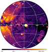 |
Fig. 6. Narrowband map in the energy range of the O VIII line as observed by eROSITA during eRASS1 in units of cts s−1 deg−2. An adaptive smoothing kernel using S/N = 15 was applied. |
4.3. Removing the contribution from the LHB
The LHB is an irregular volume filled with hot (T ∼ 0.097 keV) plasma with a typical size of ∼200 pc around the Sun (see, e.g., Yeung et al. 2023, and references therein). Being almost completely devoid of cold material, the emission from the LHB appears unaffected by absorption of X-rays.
Because of its unabsorbed nature and relatively low temperature, the LHB emission dominates mainly in the very soft X-ray band (≤0.3 keV). Zheng et al. (2024) have shown that the diffuse emission observed by eROSITA in the softer bands (0.2–0.25 keV) is indeed heavily affected by the emission from the LHB. For any study of the Galactic plasma beyond of LHB, such as the CGM and the eROSITA bubbles, it is therefore necessary to remove the foreground contribution from the LHB.
The distribution of the LHB is observed to be inhomogeneous, based on the thermal emission from the LHB detected by ROSAT in the softest energy bands (Snowden et al. 1997).
Thanks to relatively recent observations from the Diffuse X-rays from the Local Galaxy mission (DXL), Liu et al. (2017) modeled the SWCX contribution in the ROSAT R12 map and inferred the latest 3D structures of the LHB. We used the emission measure of the LHB provided in their work, assuming a constant temperature (T = 0.097 keV APEC model with Lodders (2003) abundance table) to reconstruct the observed LHB emission as observed by eROSITA in each relevant energy band. We then removed the LHB component from the maps.
Because of the relatively low temperature of LHB, the soft band is affected more than the harder bands. Figure 5 of Ponti et al. 2023a shows that the LHB generally takes a much larger fraction in the O VII narrowband flux than that in O VIII: in most regions of O VII maps, the LHB takes more than 15% of the flux, while in O VIII maps the contribution from LHB is smaller by about a factor 10.
4.4. Absorption correction
The soft X-ray spectrum is heavily affected by absorption from neutral material (Locatelli et al. 2022). To account for the absorption effect, we used the column density maps combining the HI (HI4PI Collaboration 2016) and H2 column density derived from Planck observations (Planck Collaboration Int. XLVIII 2016; Green 2018) following the recipe proposed by Willingale et al. (2013). Then, assuming Solar abundances for the absorbing medium, we derived the correction factor to be applied to deabsorb either the maps or the emission from the various emission components (see Appendix A in Locatelli et al. 2024b, for further details). The absorption correction was applied to the CGM and CXB components only, because we assumed that the SWCX and LHB components are un-absorbed. We note that the correction for the effects of absorption are negligible for column densities lower than NH ≤ 1021 cm−2 in the oxygen maps. This condition applies to all the regions included in our analysis of the temperature distribution.
4.5. Subtraction of the cosmic X-ray background (CXB)
The major contribution to the diffuse X-ray emission above ∼0.6 keV is given by the CXB (see Table 4 of Ponti et al. 2023a). Ultra-deep X-ray surveys performed with Chandra and XMM-Newton have resolved more than ∼80% and ∼92% of the CXB flux into extra-galactic discrete sources (primarily active galactic nuclei, clusters of galaxies, groups, normal galaxies, etc.) in the 0.5–2 and 2–7 keV bands, respectively (Luo et al. 2017; Brandt et al. 2021). The CXB flux is observed to be uniformly distributed, with small amplitude variations on arcminutes to degrees scales. We removed the CXB component by assuming it has constant flux on the sky, that it is absorbed by the full Galactic column density of material (computed as above), and that its spectrum can be described by a doubly broken power law (Ponti et al. 2023a). The CXB spectrum (Gilli et al. 2007) is assumed to have a photon index of Γ3 = 1.45 above 1.2 keV, of Γ2 = 1.6 between 0.4 and 1.2 keV and Γ1 = 1.9 below 0.4 keV and to have a normalization of 8.2 photons s−1 cm−2 at 1 keV.
5. The O VII and O VIII line maps of the CGM component
Figure 5 shows the half sky emission observed by eROSITA during eRASS1 within the O VII energy band, while Figure 6 shows the same map in the O VIII band. In both bands bright emission is observed at relatively high Galactic latitudes |b|≥30°, with count rates of ∼0.01 cts s−1 deg−2. Some small depressions are observed there, however they are associated with absorbing clouds (Snowden et al. 2015; Yeung et al. 2023; Ponti et al. 2023b). This indicates that, as expected, we are surrounded by hot plasma along every direction on the sky, the so called hot CGM.
As already pointed out, along most of the Galactic plane, the effect of interstellar absorption is much more relevant. Dark patches are observed nearby dark clouds, which are primarily concentrated at small latitudes. O VII and O VIII are the brightest lines observed by eROSITA in the soft band. For this reason many of the features described in both the broadband maps (Zheng et al. 2024) and in the RGB map in Fig. 2 are also evident in the narrowband maps of the oxygen lines. For instance, large-scale enhanced O VII and O VIII emission is observed both in the direction toward the Galactic center, along the footprint of the eROSITA bubbles and on smaller regions toward the anti-center (e.g., the Orion-Eridanus superbubble; the Monogem ring; the Antlia supernova remnant).
It is also possible to observe a clear trend of increasing O VIII emission closer to the Galactic plane and toward the Galactic center (Fig. 6). These large-scale features contain morphological information recently used to constrain the geometry and physical properties of the warm-hot CGM (Locatelli et al. 2024b).
6. Line ratio and pseudo-temperature maps
Figure 7 shows the ratio of the O VIII/O VII emission. The O VII and O VIII maps used to compute the ratio collect counts over a squared pixel of side length Δrpxl = 2 deg. This pixel size allows most pixels in the maps to hold C ≥ 30 counts. Under the C ≫ 1 assumption, the uncertainty related to the count can then be computed as  . We note that the only regions where the assumption is broken are those highly absorbed, primarily along the Galactic plane and toward dark clouds (Yeung et al. 2023). The Galactic plane regions are anyway not included in the quantitative analysis, and the results are presented in the following sections. We stress that, for display purposes, we have inverted the color scale, so that brighter regions correspond to a higher contribution from O VII, therefore to a lower temperature. At high Galactic latitudes |b|> 30° and away from the Galactic center l < 270°, the line ratio map appears rather smooth (with small fluctuations, that do not appear significant, see Sect. 7), with the northern hemisphere possessing slightly lower ratio. On the contrary, at high Galactic latitudes |b|> 30° toward the Galactic center l < 270°, sharp color variations are clearly observed in Fig. 7. Particularly evident is a bright (less hot) stripe running all along the edge of the northern eROSITA bubble (enclosed by the dashed white lines drawn in Fig. 7). Just inside (closer to the Galactic center) this bright stripe, a dark (hot) region is observed to run again all along the edge of the northern eROSITA bubble. Although fainter, such a dark (hot) transition layer can also be observed along a good fraction of the southern eROSITA bubble.
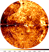 |
Fig. 7. O VIII/O VII line intensity ratio map (unitless), as observed by eROSITA during eRASS1. The contribution from CXB, LHB, foreground absorption, and instrumental background (see Sect. 4) were not removed before taking the line ratio shown in this image. An adaptive smoothing kernel using S/N = 15 was applied. The kernel used was the same for the O VII and O VIII maps. The white dashed lines are placed along the sharpest features close to the boundaries of the eROSITA bubbles. |
To better highlight this interesting feature occurring at the edge of the eROSITA bubbles, Fig. 8 shows both the X-ray continuum (0.2–2.3 keV) in green as well as the O VII to O VIII line ratio in blue and the O VII emission in red. The O VII to O VIII line ratio in blue is thus brighter whenever a source produces more O VII than O VIII, that is for lower plasma temperatures (see also Fig. 3). Fig. 8 thus clearly shows that this colder rim of emission occurs in close correspondence with the surface brightness transition used to define the edges of the eROSITA bubbles. This effect is very clear along the northern bubble but it can be followed all the way down to about −40° also in the southern bubble (Figs. 8 and 9), although partially blended with broad absorption features close to the boundary of the bubble, in projection.
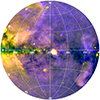 |
Fig. 8. Bright emission lines in eRASS1. The RGB map is composed of O VII (red), broadband emission in the 0.2–2.3 keV energy range (green), and the O VII/O VIII line ratio (blue). All the maps include the contribution of different components (both celestial and instrumental) and were smoothed with an adaptive kernel set to retrieve S/N threshold of 15. |
6.1. Pseudo-temperature map derived from the O VIII/O VII line ratio
Assuming that the line ratio map shown in Fig. 7 is produced by only one warm-hot plasma component, by inverting the relation in Fig. 4, from the oxygen lines ratio map, we were able to create the first temperature map of the warm-hot CGM of the Milky Way (see Fig. 9, top panel). Such a temperature map is valid only in areas where a single plasma component is emitting most of the observed photons. In other regions, where different components of comparable brightness build up the observed narrowband intensities, the derived map loses its meaning as a temperature. For this reason, a meaningful temperature map depends on an accurate selection of the emission component subject of the study, for instance, through the models and subtractions presented in Sect. 4. Additionally, absorption can severely affect the temperature map by absorbing the emission of the different lines by a different factor, therefore affecting the final temperature map. Because in several places, the assumption of a single thermal component is not true (e.g., within the footprints of the eROSITA bubbles and close to the Galactic plane, where the hot ISM could contribute to the emission), we call the map derived from the oxygen line ratio as “pseudo-temperature” map.
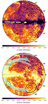 |
Fig. 9. Pseudo-temperature derived from the O lines ratio with (and without) accounting for the absorbed intensity of the line. Upper panel: Temperature map corrected for foreground absorption. This version is used for quantitative statements on the temperature throughout the paper. These maps were corrected for the LHB, CXB, SWCX, instrumental background emissions, and foreground absorption, as presented in Sect. 4 (in Fig. 7 the ratio was not corrected). The regions used for the pseudo-temperature analysis are shown in the panel below. Lower panel: Temperature map, without deabsorbing the O VII and O VIII line emission. The black circles show the regions selected for the analysis of the eROSITA bubbles and the CGM in the north and south hemispheres. The profiles shown in Figs. 12 and 13 are indicated by the transparent cyan and white regions, respectively. |
The top panel of Fig. 9 shows the pseudo-temperature 𝒯 map obtained by subtracting all components as detailed in Sect. 4. Therefore, all components discussed by Ponti et al. (2023a), apart from the CGM (composed by a hot halo, a disk-like component, and the emission of the Galactic outflow) have been removed. By looking at Fig. 1 (see also Fig. 5 of Ponti et al. 2023a), it is possible to see that, at moderate latitudes, little contribution is given to the O VII and O VIII lines by the emission attributed to the corona. This suggests that the pseudo-temperature map derived from the O VIII over O VII maps is a good proxy of the real CGM plasma temperature in regions away from the Galactic outflow and the Galactic plane. On the other hand, we expect that the additional emission induced by the Galactic outflow and the hot interstellar medium will break the initial assumption that only one thermal component is contributing to the oxygen line ratio map, therefore biasing the temperature map shown in Fig. 9 within the footprints of the eROSITA bubbles and along the Galactic plane.
The top panel of Fig. 9 shows similar structures to the ones observed in the oxygen lines ratio. In particular, the CGM pseudo-temperature appears rather uniform toward both the northern and southern hemispheres, with values on the order of 𝒯 ∼ 0.20 − 0.22 keV, respectively. A low-temperature shell (colder than the CGM) surrounds all of the northern bubble and a good fraction of the southern bubble. This shell has a considerable width, appearing as extended as ∼10° in several places. We note that, just inside this colder shell, the temperature rises again to temperatures higher than the surrounding CGM. Again, this interior and hotter shell surround all of the northern bubble as well as a good fraction of the southern one (Fig. 9).
The question arises of whether the LHB alone can be attributed to the O VIII/O VII line-ratio transition at the eROSITA bubbles. A 0.1 keV LHB can be approximated to produce only O VII but not O VIII. Assuming a single-temperature CGM that gives a uniform O VIII/O VII line ratio across the sky, adding such a LHB component always decreases the line ratio, more at locations where the LHB emission measure is high. Since the Liu et al. (2017) LHB model shows a lower emission measure at l ≳ 300° (near eROSITA bubbles) compared to the rest of the western Galactic hemisphere, one should see a lower O VII (hence higher O VIII/O VII) in the eROSITA bubbles compared to outside. While we model the LHB emission according to the best available information, deviations of ±15% from a uniform LHB temperature have been recently found (Yeung et al. 2023) in a few directions toward giant molecular clouds, at odds with the model used in this work. Further improvements in the knowledge of the LHB thermodynamics will be beneficial to the analysis presented in this work.
In addition, we emphasize that our results and interpretations concerning the pseudo-temperature rely on the assumption of a single-temperature, collisionally ionized plasma. In non-equilibrium scenarios, the observed lowering of the line ratio in the shell could be due to an under-ionization state rather than a lower temperature. As the ionization properties depend on the emission model, we present our results only based on the stated assumptions.
The bottom panel of Fig. 9 shows how the temperature map changes once the correction for absorption is not applied. As expected, only in highly absorbed regions (i.e., along the Galactic plane and toward dark clouds) do the corrections become relevant.
7. Constraining the temperature distribution of the circumgalactic medium
7.1. Circumgalactic medium temperature distribution on small scales
To constrain the pseudo-temperature distribution of the CGM away from the Galactic plane and center, we selected two circular regions centered at (l,b) = (220,+50) and (l,b) = (230,–50) and with radii of 20 degrees (black solid wide circles in Fig. 9, bottom panel). Two additional regions at coordinates (l,b) = (340,+40) and (l,b) = (340,–30) with radii of 10 degrees were also considered to study the pseudo-temperature within the eROSITA bubbles (black solid small circles in Fig. 9, bottom panel).
Choosing moderate- and high-latitude regions minimizes potential systematic uncertainties in the oxygen ratio introduced by the absorption model used to retrieve the unabsorbed CGM emission in both oxygen bands (see Appendix A). Figure 10 shows the probability distribution function of the pseudo-temperature within the selected regions, obtained using a pixel side length of Δrpxl = 2 deg. The distributions from the northern and southern hemispheres are shown by the black solid and red dashed lines, respectively. In Fig. 10, the horizontal error bars show the root-mean-square (rms) value σrms of the pseudo-temperature uncertainty in the regions considered.
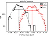 |
Fig. 10. Probability distribution function (PDF) of the pseudo-temperature derived in the north and south CGM regions (black solid and red dashed lines, respectively; see footprints in the lower panel of Fig. 9). The thin solid lines show Gaussian fits of the temperature distributions. The vertical dashed lines show the median values of the distribution with the uncertainty on the mean bracketed by the filled vertical regions. |
The value σrms happens to be similar to the standard deviation std(𝒯) of the pseudo-temperature map computed in the same region (i.e., σrms ≃ std(𝒯)), in both the north and south regions. We conclude that the CGM pseudo-temperature can be considered uniform over the regions considered, that is, between 2 and 20 deg scales, given the statistical uncertainties on the pseudo-temperature values. Any intrinsic fluctuation ΔT would in fact contribute to the overall spread of the distribution std(𝒯) following (e.g., Vaughan et al. 2003)
 (1)
(1)
Therefore, provided std(𝒯)≃σrms, we constrain any intrinsic pseudo-temperature fluctuation to be ΔT ≤ Δ𝒯 ≤ σrms = 0.007 keV on Δθ ≃ 2 − 20 deg in the CGM regions. The fractional fluctuation with respect to the average pseudo-temperature Δ𝒯/⟨𝒯⟩ (reported below in Sect. 7.2) amounts to Δ𝒯/⟨𝒯⟩≤4% for both the north and south regions. In particular, in the south region we find Δ𝒯 = 0.0062 keV (i.e., Δ𝒯 > 0), hinting to a detected fluctuation of the pseudo-temperature of Δ𝒯/⟨𝒯⟩ = 2.7%. Due to the eROSITA scanning strategy, the southern hemisphere is characterized by a higher exposure than the north, thus providing relatively deeper data.
We assessed the statistical uncertainty on the potential fluctuation by exploiting both a jackknife resampling and a bootstrap of the pseudo-temperature distribution. The derived statistics on the simulated distributions are consistent between the two methods. We obtain that the values std(𝒯) and σrms of the simulated distributions vary (one standard deviation) by 3.7% and 1.4% of their expected value, respectively. We derive Δ𝒯 = 0.0062 ± 0.0004 keV (statistical) by propagating the uncertainties. Additional systematic biases however, may be introduced by the modeling of the back- and foreground components subtracted to retrieve the CGM intensity. By switching on and off the subtraction of the different components (i.e., CXB, LHB, SWCX) and increasing their flux by an arbitrary 10%, we find a shift in the detected excess of ±0.0013 keV. The uncertainty on the fluctuations is then dominated by the systematic component. We obtain Δ𝒯 = 0.0062 ± 0.0004 keV (statistical) ±0.0013 keV (systematic), translating to Δ𝒯/⟨𝒯⟩ = 2.7%±0.2% (statistical) ±0.6% (systematic). The detected fluctuation thus seems significant (with respect to zero). We only investigated systematic uncertainties by modifying the relative importance of back- and foreground components without changing their morphology. For this reason, we are still cautious about the source of this signal. Further investigations exploiting the full amount of the eROSITA data (ongoing) will be able to confirm or disprove the origin of this excess in the scatter of the line ratio distribution and better assess which fraction of the observed fluctuation has to be ascribed to other components. This measure however, sets a tight upper limit to the temperature variations of the warm-hot CGM.
7.2. North-south asymmetry in the pseudo-temperature distribution of the CGM
As already pointed out when describing Fig. 7, we note that the CGM in the southern hemisphere appears hotter (i.e., higher line ratio) than its northern counterpart. From the oxygen pseudo-temperature map, the derived mean pseudo-temperature values are ⟨𝒯⟩ = 0.195 ± 0.001 keV and ⟨𝒯⟩ = 0.218 ± 0.001 keV for the north and south regions respectively. The quoted uncertainties indicate the error on the mean. The median pseudo-temperatures are equal to the mean pseudo-temperatures within uncertainties. The difference between north and south pseudo-temperature is thus Δ𝒯 = 0.024 ± 0.001 keV, where the uncertainty has been obtained from the quadrature of the mean pseudo-temperature uncertainties of the north and south samples. Thus, we find a significant difference of Δ𝒯/⟨𝒯⟩≃12% in the pseudo-temperature of the hot CGM when comparing representative regions in the north and south Galactic hemispheres. This difference is larger than the sum of statistical and systematic uncertainties (see Appendix A), and we thus interpret it as a physical, real effect.
This then suggests that the pseudo-temperature of the CGM has variations as large as ∼12% on scales of several tens of degrees. In contrast, when looking at angular scales on the order of ∼2 − 20°, then the pseudo-temperature distribution is consistent with being normal and shows variations as small as 2 − 3%, or in any case smaller than Δ𝒯 ≤ 4%.
8. Constraining the pseudo-temperature distribution within the eROSITA bubbles
Figure 11 shows the probability distribution function of the pseudo-temperature within two circular regions inside the northern and southern eROSITA bubbles (in black and red, respectively). We stress again that, within this region, at least two thermal components (i.e., the emission from the eROSITA bubbles, plus the emission from the other parts of the CGM) contribute to the total emission. Therefore, the pseudo-temperature derived from the line ratio must be biased. In particular, as shown in Figs. 3 and 4, the pseudo-temperatures derived from the oxygen line ratio are unable to trace plasma hotter than T ∼ 0.3 keV. The pseudo-temperatures derived from the oxygen line ratio are observed to be ⟨𝒯⟩ = 0.211 ± 0.001 keV and ⟨𝒯⟩ = 0.217 ± 0.001 keV for the northern and southern bubbles, respectively. These values are surprisingly similar to the temperatures derived for the CGM outside the eROSITA bubbles, indicating that the oxygen line ratio is not sensitive to the presence of a hotter component within the bubbles (see Fig. 1). Therefore, although the absolute value of the pseudo-temperature might be biased inside the eROSITA bubbles (because the presence of a hotter component is not traced), we expect that intrinsic variations of the temperature of the eROSITA bubbles would induce a spread in the distribution of oxygen line ratio and, consequently, on the pseudo-temperatures derived from the latter.
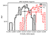 |
Fig. 11. Probability distribution function (PDF) of the pseudo-temperature in the north and south regions inside the eROSITA bubbles (black solid and red dashed lines, respectively; see footprints in the lower panel of Fig. 9). |
Figure 11 shows that the mean uncertainty on the value of the pseudo-temperature is significantly smaller than the pseudo-temperature standard deviation σrms < std(𝒯), indicating that there are significant pseudo-temperature variations observed. The typical error bars within these regions inside the eROSITA bubbles are smaller than the CGM regions, thanks to the brighter emission characterizing the bubbles compared to the background (faint) CGM. This suggests significant temperature variations are observed on small (∼2 − 10 degrees) scales within the eROSITA bubbles. We obtain std(𝒯) = 0.007 keV in both regions and σrms = 0.003, 0.005 keV in the north and south region respectively. From Eq. (1), we derive Δ𝒯 = 0.006, 0.004 keV. Compared to the average values ⟨𝒯⟩ = 0.2262 ± 0.0007 keV and ⟨𝒯⟩ = 0.2340 ± 0.0007 keV in the north and south regions within the eROSITA bubbles, the relative strength of the excess scatter is Δ𝒯/⟨𝒯⟩ = 2.7, 1.9%, respectively. The relative excess scatter thus shows similar strength inside and outside (see Sect. 7) the eROSITA bubbles.
Potential deviations from a normal distribution (solid lines in Fig. 10) has been tested through a Kolmogorov–Smirnov (KS) test on both the north and south samples. The tested hypothesis is that of an underlying normal distribution of the sample. Both 𝒯 and log𝒯 distributions have been tested using the KS. The test hypothesis is considered as rejected for p < 0.05. The resulting p-values do not reject the null hypothesis in all cases. The pseudo-temperature distributions are thus consistent with a normal distribution. A fit using a normal distribution is also shown (solid lines in Fig. 10).
8.1. Pseudo-temperature variations across the eROSITA bubbles
In Sect. 6, we discussed the presence of pseudo-temperature variations across the edges of the eROSITA bubbles. To investigate in more detail the trend across the edge of the eROSITA bubbles, we drew pseudo-temperature profiles, from (l, b) = (350, ±15) to (l, b) = (250, ±60). The two profiles shown in Fig. 12 are thus symmetric with respect to the Galactic plane, and their path in the sky is shown in the lower-left corner, and the bottom panel of Fig. 9. Δθ is the angle [deg] between a given point in the sky, along the profile, and the point of lower absolute latitude |b|.
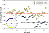 |
Fig. 12. Pseudo-temperature profiles across the eROSITA bubbles. The paths are also shown as cyan transparent regions in the bottom panel of Fig. 9. |
The two profiles in Fig. 12 show different ratios between the regions inside (small Δθ) and outside (large Δθ, i.e., the CGM) the eROSITA bubbles. In particular, the northern bubble (blue dots) shows a significant increase toward the inner regions, while a milder transition characterized the southern bubble (yellow squares). We stress once again that, as indicated by Fig. 1, the plasma inside the eROSITA bubbles might have a contribution from a hotter component, which is not traced by the oxygen line ratio. Therefore, the mean temperature inside the bubbles is likely larger than the pseudo temperature shown in Fig. 12.
Figure 12 shows clear pseudo-temperature variations at the edges of the eROSITA bubbles. This transition happens at higher (absolute) latitudes in the northern bubble compared to the southern one. In other words, the X-ray emission from the bubbles is not symmetric with respect to the Galactic equator, with the northern bubble being brighter and more evident at higher latitudes. Complementary, while the foreground absorption in the northern hemisphere reaches NH = 1021 cm−2 at b ≃ 30 − 40 deg, the southern hemisphere is less absorbed, with the same NH being limited to b > −20 deg. This allows us to extend the investigation on the pseudo-temperature in the southern bubble to regions closer to the Galactic plane or the Galactic center. In Fig. 12, we partially hid the data points characterized by a column density NH > 1021 cm−2, thus potentially biased by systematic on the absorption model.
The colder shell at about the boundary of the bubbles can be recognized by the steep drop at around Δθ ≃ 50 − 60 deg from the path origin. In the south, the regions well inside the bubble are characterized by a higher average pseudo-temperature than in the north. A constant value is then observed well outside the boundaries eventually (l ∼ 240 − 210 deg) matching the same level of the CGM regions (dashed lines).
The regions around the boundary of the bubbles show a systematic pseudo-temperature drop in both hemispheres when compared to the respective CGM values. The drop (i.e., the colder shell) is more evident in the north and is also present in the south. At the same time, a small but significant enhancement is observed Δθ = 10 − 20 deg before the drop in both hemispheres. Strong deviations from homogeneity are found within the boundaries of the bubbles. While these inhomogeneities prevent us from characterizing the details of a putative pseudo-temperature jump, we find evidence for a higher pseudo-temperature and broad spatial variations of 𝒯 inside the bubbles compared to the outer regions.
Given the brighter emission of the northern bubble, we further inspected the inhomogeneities through different profiles across it, as shown in the panels of Fig. 12 (the profiles are also charted as a white transparency in the bottom panel of Fig. 9). All the profiles have origin at (l, b) = (350, 35). From these profiles, the features described above (e.g., the pseudo-temperature enhancement, the colder shell, the constant and scattered value at large Δθ, and the large and coherent variations inside the bubbles) are all evident and highly significant. We note that along the profile encompassing the highest latitudes (Fig. 13, top panel), the pseudo-temperature shows a significant and increasing trend with respect to the average CGM value. This confirms that the cold-warm shell noticed in the line ratio and pseudo-temperature maps is statistically significant.
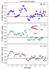 |
Fig. 13. Pseudo-temperature profiles across the northern eROSITA bubble. The paths are also shown as white transparent regions in the bottom panel of Fig. 9. |
9. Discussion
Thanks to the eROSITA energy resolution, we could derive the first half sky maps in narrow energy bands characteristic of some of the most prominent soft X-ray emission lines. These narrowband maps allowed us to detect several known features, reveal new structures, and use line ratio maps to derive a pseudo-temperature map of the CGM of the Milky Way.
9.1. On the pseudo-temperature distribution of the CGM
The study of the soft X-ray emission lines (and their ratio), has allowed us to place constraints on the pseudo-temperature distribution of the CGM. We observe that on small angular scales, up to ∼20°, the CGM pseudo-temperature shows an overall normal distribution with fluctuations from the expected value on the order of a few percent, not accounted for by our modeling. Conservatively, an overall upper limit to the intrinsic pseudo-temperature fluctuations on the order of Δ𝒯 ≤ 4% can be considered. At first sight, this may appear in contrast with simulations of galaxies, predicting log-normal distributions of the CGM pseudo-temperatures and significant pseudo-temperature fluctuations from different regions in the sky. However, we note that we trace the pseudo-temperature distribution based only on the ratio of the O VIII and O VII lines, which are sensitive to the hotter component of the CGM. Therefore, we cannot exclude that the real pseudo-temperature distribution is actually skewed toward lower pseudo-temperature (e.g., traced by O VI), but we are insensitive to those CGM phases here.
By comparing the CGM pseudo-temperature in the northern and southern hemispheres, we also observed significant pseudo-temperature variations on scales larger than ∼20°, on the order of ∼12%. Significant pseudo-temperature variations are also observed when comparing the interior of the eROSITA bubbles with the high Galactic latitude region away from the Galactic center. However, the presence of an additional hotter component prevents us from quantifying this pseudo-temperature jump in an unbiased way. Therefore, the study of the line ratio suggests that the CGM undergoes significant pseudo-temperatures variations of at least ∼12% on angular scales of several tens of degrees, while we observe that on smaller angular scales (∼2 − 20°) the pseudo-temperature is significantly smaller, and on the order of a few percent.
9.2. An additional and hotter plasma component inside the eROSITA bubbles
In the previous Sect. 8, we detected clear pseudo-temperature variations at the edges of the eROSITA bubbles. The pseudo-temperature map, derived from the oxygen line ratio, indicates pseudo-temperatures of 𝒯 ∼ 0.21 − 0.22 keV and 𝒯 ∼ 0.19 − 0.22 keV for the region inside and outside the eROSITA bubbles, respectively. This appears in agreement with some recent results based on the analysis of Suzaku spectra (Gupta et al. 2023), which find a pseudo-temperature of the plasma inside the bubbles to be consistent with 𝒯 ∼ 0.2 keV, although with a significant overabundance of neon to oxygen of ∼2. We reiterate that the oxygen line ratio is not very sensitive to any component hotter than T ∼ 0.3 keV, as suggested by previous studies of the same Suzaku data, which did not require neon overabundance (Kataoka et al. 2018). To discriminate between these different hypotheses, a full characterization of the spectra from the inside and outside of the eROSITA bubbles is necessary (e.g., Fig. 1).
9.3. A shell surrounding the eROSITA bubbles
The investigation of the oxygen line ratio suggests the presence of a shell of colder material, with an inner hotter stripe, close to the edge of the eROSITA bubbles, defined as the drop in surface brightness. The shell appears to wrap most of the northern bubble and a good fraction of the southern bubble closer to the plane. The origin of such a shell is still unclear. Colder phases as transition layers between an expanding bubble and the interstellar medium are typically observed in superbubbles, where a colder and high-density shocked interstellar gas is contained between the forward shock and the contact discontinuity separating it from the hotter and more rarefied shocked stellar wind (Weaver et al. 1977). This colder and high-density shell forms because of radiative losses, which become relevant as the superbubble expands into the interstellar medium.
Clearly, the example of superbubbles shows that an outflow interacting with the colder ambient gas can form a shell. However, the conditions experienced by the putative Galactic outflow, which might have shaped the eROSITA bubbles, are probably closer to the ones in galactic outflows observed in star-forming and starburst galaxies, where the assumption of a homogeneous ambient medium creating a homogeneous shell in all direction is likely, not true. The typical scale height of galactic outflows is significantly larger than their galactic disks. Therefore, the galactic plane is likely helping in impeding the expansion of the outflow along the plane and in collimating the outflow into a bipolar feature, which is expanding more toward directions where there is a significant drop in the density of the environment (the CGM). Because of the significant drop in the density of the environment (the CGM), outflows from star-forming galaxies are not expected to produce a colder cap, as observed in superbubbles. Instead, such denser and colder phases might be developed at the boundary between the outflow and the galactic plane and to trace the edges of the outflow up to several kiloparsecs above the Galactic plane. Thus, within the framework of a Galactic outflow, it is puzzling that the colder shell can be traced all the way to the top of the northern eROSITA bubble.
The observation of a shell reaching very high Galactic latitudes might be related to either entrainment and mixing between the hot and colder phases of the outflow or to projection effects. The geometry of the outflow may be different from the one assumed in Predehl et al. (2020) because the eROSITA bubbles are so extended in the sky that the upper portion of this layer, which appears at Galactic latitudes of b ∼ 60° or more, may be associated with the near side of the Galactic outflow, which is so extended to fill the sky above us. We note that in such a scenario, it is somewhat natural to expect that this colder shell will trace the edges of the eROSITA bubbles closer to the Galactic plane. A colder shell might be present all along the envelope around the eROSITA bubble and closer to the Galactic plane, but to appear clearer at its edges because of projection effects. If so, then no cap would be present at the top of the Galactic outflow and the colder shell observed in our maps would be due to the projection of the near side of the outflow, just a few kiloparsecs above the Galactic plane.
This prompts further consideration of the connections between eROSITA bubbles and other known large-scale structures such as the North Pole Spur (NPS). This extended X-ray arc, previously detected by ROSAT (Snowden et al. 1997) emerges from the eastern Galactic plane and gradually fades as it extends out from the plane. The NPS can be considered as part of the northern eROSITA bubble. A bright and extended radio structure known as Loop-I has been associated to the NPS (Berkhuijsen et al. 1971; Haslam et al. 1974; Sofue & Reich 1979; Vidal et al. 2015; Planck Collaboration XXV 2016). However, it is unclear whether the radio structure Loop-I and the northern eROSITA bubble share a common origin. The high radio intensity from the low-latitude ISM regions complicates the determination of the origin of Loop I. There is still an open debate on the origin of the Loop-I/NPS feature. While some studies propose a Galactic Center (GC) origin (Sofue 1977, 2000; Bland-Hawthorn & Cohen 2003; Kataoka et al. 2013), others propose a local origin (Egger & Aschenbach 1995; Dickinson 2018). Currently, both scenarios are still consistent with observations. While the appearent lack of a corresponding southern feature for NPS/Loop-I posed a challenge for GC origin, the reassessment of the South Pole Spur (SPS) in planck map (Planck Collaboration XXV 2016) seemed to reduce the discrepancy with GC models. We note here that this radio-detected SPS aligns well with southern eROSITA bubbles in the projection as viewed from Earth (see a review of Sarkar 2024).
Of course, more work is needed to clarify the three-dimensional geometry of the eROSITA bubbles and the origin of the features observed here. What seems clear from the data is the pseudo-temperature variation across the edges of the bubbles, indicating the presence of a shell.
10. Conclusions
We investigated the eROSITA half sky maps within narrow energy bands characteristic of the brightest soft X-ray line transitions. Our conclusions are as follows:
-
We subtracted the non-CGM components from soft X-ray emission lines (O VII and O VIII) and corrected the maps for the effects of absorption to determine the emission from the hot plasma associated with the CGM;
-
Toward regions with little effects due to absorption, we derived maps of the pseudo-temperature of the CGM plasma from the O VIII/O VII line ratio, which is a good tracer of the pseudo-temperature of the warm-hot CGM unperturbed by the Galactic outflow;
-
We constrained the CGM temperature fluctuations for the first time on relatively small (∼2 − 20°) and large scales. The CGM pseudo-temperature shows fluctuations not accounted for by our background and foreground modeling, on the order of ∼3%, and with an upper limit of Δ𝒯/𝒯 ≤ 4% on angular scales between ∼2 and ∼20°. Instead, the CGM temperature shows variations as large as ∼12% when comparing the northern and southern hemispheres, therefore indicating that pseudo-temperature fluctuations are indeed present on large angular scales (i.e., ≫20°);
-
Toward the northern and southern eROSITA bubbles we detected significant pseudo-temperature fluctuations of order 2 − 3% of the average values, indicating significant temperature fluctuations toward the interior of the bubbles.
-
The line ratio map shows significant variations at the edges of the eROSITA bubbles, suggesting the presence of a shell of lower values at the edge of the outflow. In particular, when the line ratio map was translated into a pseudo-temperature map, we could see that the interior of the eROSITA bubbles appears hotter than the surrounding CGM. Approaching the edge from the interior of the bubble, we observe a rise in the pseudo-temperature, followed by a significant drop, to then become hotter again, with a pseudo-temperature consistent with the surrounding CGM. This suggests the presence of a shell of cooler material present at the edge of the bubbles or of a separate process (not modeled in this work) affecting the different metal ionization states.
For simplicity, we refer to temperature as kT or just T throughout the paper. Therefore, we report all temperatures T using keV units.
Acknowledgments
This work is based on data from eROSITA, the soft X-ray instrument aboard SRG, a joint Russian-German science mission supported by the Russian Space Agency (Roskosmos), in the interests of the Russian Academy of Sciences represented by its Space Research Institute (IKI), and the Deutsches Zentrum für Luft- und Raumfahrt (DLR). The SRG spacecraft was built by Lavochkin Association (NPOL) and its subcontractors, and is operated by NPOL with support from the Max Planck Institute for Extraterrestrial Physics (MPE). The development and construction of the eROSITA X-ray instrument was led by MPE, with contributions from the Dr. Karl Remeis Observatory Bamberg & ECAP (FAU Erlangen-Nuernberg), the University of Hamburg Observatory, the Leibniz Institute for Astrophysics Potsdam (AIP), and the Institute for Astronomy and Astrophysics of the University of Tübingen, with the support of DLR and the Max Planck Society. The Argelander Institute for Astronomy of the University of Bonn and the Ludwig Maximilians Universität Munich also participated in the science preparation for eROSITA. The eROSITA data shown here were processed using the eSASS/NRTA software system developed by the German eROSITA consortium. We acknowledge financial support from the European Research Council (ERC) under the European Union’s Horizon 2020 research and innovation program Hot- Milk (grant agreement No 865637). GP acknowledges support from Bando per il Finanziamento della Ricerca Fondamentale 2022 dell’Istituto Nazionale di Astrofisica (INAF): GO Large program and from the Framework per l’Attrazione e il Rafforzamento delle Eccellenze (FARE) per la ricerca in Italia (R20L5S39T9). MF and MY acknowledge support from the Deutsche Forschungsgemeinschaft through the grant FR 1691/2-1.
References
- Allen, B., Hoak, D., Hong, J., et al. 2019, in Asteroid Science in the Age of Hayabusa2 and OSIRIS-REx, LPI Contributions, 2189, 2009 [NASA ADS] [Google Scholar]
- Anders, E., & Grevesse, N. 1989, Geochim. Cosmochim. Acta, 53, 197 [Google Scholar]
- Balucinska-Church, M., & McCammon, D. 1992, ApJ, 400, 699 [Google Scholar]
- Berkhuijsen, E. M., Haslam, C. G. T., & Salter, C. J. 1971, A&A, 14, 252 [NASA ADS] [Google Scholar]
- Bland-Hawthorn, J., & Cohen, M. 2003, ApJ, 582, 246 [Google Scholar]
- Brandt, W. N., Ni, Q., & The Xmm-Servs Team 2021. Am. Astron. Soc. Meet. Abstr., 53, 209.01 [Google Scholar]
- Brunner, H., Liu, T., Lamer, G., et al. 2022, A&A, 661, A1 [NASA ADS] [CrossRef] [EDP Sciences] [Google Scholar]
- Das, S., Mathur, S., Nicastro, F., & Krongold, Y. 2019a, ApJ, 882, L23 [NASA ADS] [CrossRef] [Google Scholar]
- Das, S., Mathur, S., Gupta, A., Nicastro, F., & Krongold, Y. 2019b, ApJ, 887, 257 [NASA ADS] [CrossRef] [Google Scholar]
- Dickinson, C. 2018, Galaxies, 6, 56 [NASA ADS] [CrossRef] [Google Scholar]
- Egger, R. J., & Aschenbach, B. 1995, A&A, 294, L25 [NASA ADS] [Google Scholar]
- Gilli, R., Comastri, A., & Hasinger, G. 2007, A&A, 463, 79 [NASA ADS] [CrossRef] [EDP Sciences] [Google Scholar]
- Górski, K. M., Hivon, E., Banday, A. J., et al. 2005, ApJ, 622, 759 [Google Scholar]
- Green, G. 2018, J. Open Source Softw., 3, 695 [NASA ADS] [CrossRef] [Google Scholar]
- Gupta, A., Mathur, S., Kingsbury, J., Das, S., & Krongold, Y. 2023, Nat. Astron., 7, 799 [NASA ADS] [CrossRef] [Google Scholar]
- Haslam, C. G. T., Wilson, W. E., Graham, D. A., & Hunt, G. C. 1974, A&AS, 13, 359 [NASA ADS] [Google Scholar]
- Henley, D. B., & Shelton, R. L. 2012, ApJS, 202, 14 [NASA ADS] [CrossRef] [Google Scholar]
- Henley, D. B., Shelton, R. L., Kwak, K., Joung, M. R., & Mac Low, M.-M. 2010, ApJ, 723, 935 [NASA ADS] [CrossRef] [Google Scholar]
- HI4PI Collaboration (Ben Bekhti, N., et al.) 2016, A&A, 594, A116 [NASA ADS] [CrossRef] [EDP Sciences] [Google Scholar]
- Joubaud, T., Grenier, I. A., Ballet, J., & Soler, J. D. 2019, A&A, 631, A52 [NASA ADS] [CrossRef] [EDP Sciences] [Google Scholar]
- Kataoka, J., Tahara, M., Totani, T., et al. 2013, ApJ, 779, 57 [NASA ADS] [CrossRef] [Google Scholar]
- Kataoka, J., Sofue, Y., Inoue, Y., et al. 2018, Galaxies, 6, 27 [Google Scholar]
- Knies, J. R. 2022, PhD thesis, Friedrich-Alexander-Universität Erlangen-Nürnberg (FAU), Germany [Google Scholar]
- Kuntz, K. D. 2019, A&ARv, 27, 1 [NASA ADS] [CrossRef] [Google Scholar]
- Liu, W., Chiao, M., Collier, M. R., et al. 2017, ApJ, 834, 33 [Google Scholar]
- Locatelli, N., Ponti, G., & Bianchi, S. 2022, A&A, 659, A118 [NASA ADS] [CrossRef] [EDP Sciences] [Google Scholar]
- Locatelli, N., Ponti, G., Merloni, A., et al. 2024a, A&A, 688, A85 [NASA ADS] [CrossRef] [EDP Sciences] [Google Scholar]
- Locatelli, N., Ponti, G., Zheng, X., et al. 2024b, A&A, 681, A78 [NASA ADS] [CrossRef] [EDP Sciences] [Google Scholar]
- Lodders, K. 2003, ApJ, 591, 1220 [Google Scholar]
- Lodders, K., Palme, H., & Gail, H. P. 2009, Landolt Boernstein, 4B, 712 [Google Scholar]
- Luo, B., Brandt, W. N., Xue, Y. Q., et al. 2017, ApJS, 228, 2 [Google Scholar]
- Merloni, A., Lamer, G., Liu, T., et al. 2024, A&A, 682, A34 [NASA ADS] [CrossRef] [EDP Sciences] [Google Scholar]
- Miller, M. J., & Bregman, J. N. 2015, ApJ, 800, 14 [NASA ADS] [CrossRef] [Google Scholar]
- Planck Collaboration XXV. 2016, A&A, 594, A25 [NASA ADS] [CrossRef] [EDP Sciences] [Google Scholar]
- Planck Collaboration Int. XLVIII. 2016, A&A, 596, A109 [NASA ADS] [CrossRef] [EDP Sciences] [Google Scholar]
- Ponti, G., Zheng, X., Locatelli, N., et al. 2023a, A&A, 674, A195 [NASA ADS] [CrossRef] [EDP Sciences] [Google Scholar]
- Ponti, G., Sanders, J. S., Locatelli, N., et al. 2023b, A&A, 670, A99 [NASA ADS] [CrossRef] [EDP Sciences] [Google Scholar]
- Predehl, P., Sunyaev, R. A., Becker, W., et al. 2020, Nature, 588, 227 [CrossRef] [Google Scholar]
- Predehl, P., Andritschke, R., Arefiev, V., et al. 2021, A&A, 647, A1 [EDP Sciences] [Google Scholar]
- Sarkar, K. C. 2024, A&ARv, 32, 1 [NASA ADS] [CrossRef] [Google Scholar]
- Smith, R. K., Brickhouse, N. S., Liedahl, D. A., & Raymond, J. C. 2001, ApJ, 556, L91 [Google Scholar]
- Snowden, S. L., Egger, R., Freyberg, M. J., et al. 1997, ApJ, 485, 125 [Google Scholar]
- Snowden, S. L., Koutroumpa, D., Kuntz, K. D., Lallement, R., & Puspitarini, L. 2015, ApJ, 806, 120 [NASA ADS] [CrossRef] [Google Scholar]
- Sofue, Y. 1977, A&A, 60, 327 [NASA ADS] [Google Scholar]
- Sofue, Y. 2000, ApJ, 540, 224 [NASA ADS] [CrossRef] [Google Scholar]
- Sofue, Y., & Reich, W. 1979, A&AS, 38, 251 [NASA ADS] [Google Scholar]
- Sunyaev, R., Arefiev, V., Babyshkin, V., et al. 2021, A&A, 656, A132 [NASA ADS] [CrossRef] [EDP Sciences] [Google Scholar]
- Vaughan, S., Edelson, R., Warwick, R. S., & Uttley, P. 2003, MNRAS, 345, 1271 [Google Scholar]
- Vidal, M., Dickinson, C., Davies, R. D., & Leahy, J. P. 2015, MNRAS, 452, 656 [NASA ADS] [CrossRef] [Google Scholar]
- Weaver, R., McCray, R., Castor, J., Shapiro, P., & Moore, R. 1977, ApJ, 218, 377 [Google Scholar]
- Willingale, R., Starling, R. L. C., Beardmore, A. P., Tanvir, N. R., & O’Brien, P. T. 2013, MNRAS, 431, 394 [Google Scholar]
- Yeung, M. C. H., Freyberg, M. J., Ponti, G., et al. 2023, A&A, 676, A3 [NASA ADS] [CrossRef] [EDP Sciences] [Google Scholar]
- Yoshino, T., Mitsuda, K., Yamasaki, N. Y., et al. 2009, PASJ, 61, 805 [NASA ADS] [Google Scholar]
- Zheng, X., Ponti, G., Freyberg, M., et al. 2024, A&A, 681, A77 [NASA ADS] [CrossRef] [EDP Sciences] [Google Scholar]
- Zonca, A., Singer, L., Lenz, D., et al. 2019, J. Open Source Softw., 4, 1298 [Google Scholar]
Appendix A: Fore ground absorption
The flux of an emission line is contributed by different sources, as discussed above. Some of these sources, such as the CXB and the CGM (i.e., the object of our study) are also absorbed by foreground cold(er) layers of material. In addition, the absorption coefficient depends on the energy considered (Balucinska-Church & McCammon 1992). To correctly interpret the line ratio between different emission lines it is thus necessary to account for the fraction of absorbed ration and add it back to the total emitted line flux. In order to do so, a model for the absorption column density (and metal content) has to be assumed. The final line ratio thus depends on the absorption model, and potentially introduces systematics in the results. The absorption model adopted in this work is the same as the one described in Locatelli et al. (2024b), we refer to that work for further details on the model. In Fig. 9 we plot a pseudo-temperature map (upper panel) derived from a line ratio where we did not added back the absorbed emission, and thus does not depend on the absorption model. By comparing it with Fig. 7 (we plot one versus the other in the lower panel of Fig. 9) we show that for all absolute Galactic latitudes |b|≥20 deg, the deviation introduced by the absorption model are negligible. This is mostly due to the relatively small column densities of absorbing material found at these latitudes. This also means that any systematic deviation introduced by the absorption model will be smaller than the deviation from unity seen in the lower panel Fig. 9 at a given latitude. Given that our representative samples in both the northern and southern hemispheres have been drawn at |b|> 30 deg for all pixels, we constrain any systematic deviation introduced by the absorption model in our samples to Δ𝒯/⟨𝒯⟩< 5%.
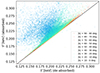 |
Fig. A.1. Pseudo-temperature values derived by the absorbed (upper panel) vs the de-absorbed lines (see Fig. 7). The pixel values are colored according to their absolute Galactic latitude, in steps of 10 deg, as labeled. All |b|> 30 deg values deviate from the 1:1 relation (black solid line) to less than 5% of their value. |
All Tables
Transitions considered in this work and corresponding energy band selected to extract photon lists and to create the corresponding images.
All Figures
|
Fig. 1. Spectra of the diffuse emission observed by eROSITA within two sky patches of 3° ×3° each. Upper panel: Observed and modeled spectrum of the sky region at |
| In the text | |
|
Fig. 2. Bright emission lines in eRASS1. The RGB map is composed of the broadband maps at 0.20–0.25 keV (red, Zheng et al. 2024) and 0.2–2.3 keV (green, Zheng et al. 2024), and the narrowband O VIII images (blue, this work). All the maps include the contribution of different components (both celestial and instrumental), and were smoothed with an adaptive kernel set to retrieve a S/N threshold of 15. |
| In the text | |
|
Fig. 3. Ionization fraction of oxygen as a function of temperature (from AtomDB, see Smith et al. 2001). The vertical dotted lines in gray show the typical temperatures of LHB (T = 0.097 keV); CGM (T = 0.15 keV); and eROSITA bubbles (assumed to be T = 0.3 keV). |
| In the text | |
|
Fig. 4. Narrowband intensity ratio as a function of temperature, and absolute and relative metal abundances (as labeled, from AtomDB Smith et al. 2001, and convolved with the eROSITA spectral resolution). The shaded areas encompass 2, 10, 25, 75, 90, and 98% of the distribution of the narrowband intensity ratio analyzed in this work (an image of the data is presented in the top panel of Fig. 9). |
| In the text | |
|
Fig. 5. Narrowband map in the energy range of the O VII line as observed by eROSITA during eRASS1 in units of cts s−1 deg−2. An adaptive smoothing kernel using S/N = 15 was applied. |
| In the text | |
|
Fig. 6. Narrowband map in the energy range of the O VIII line as observed by eROSITA during eRASS1 in units of cts s−1 deg−2. An adaptive smoothing kernel using S/N = 15 was applied. |
| In the text | |
|
Fig. 7. O VIII/O VII line intensity ratio map (unitless), as observed by eROSITA during eRASS1. The contribution from CXB, LHB, foreground absorption, and instrumental background (see Sect. 4) were not removed before taking the line ratio shown in this image. An adaptive smoothing kernel using S/N = 15 was applied. The kernel used was the same for the O VII and O VIII maps. The white dashed lines are placed along the sharpest features close to the boundaries of the eROSITA bubbles. |
| In the text | |
|
Fig. 8. Bright emission lines in eRASS1. The RGB map is composed of O VII (red), broadband emission in the 0.2–2.3 keV energy range (green), and the O VII/O VIII line ratio (blue). All the maps include the contribution of different components (both celestial and instrumental) and were smoothed with an adaptive kernel set to retrieve S/N threshold of 15. |
| In the text | |
|
Fig. 9. Pseudo-temperature derived from the O lines ratio with (and without) accounting for the absorbed intensity of the line. Upper panel: Temperature map corrected for foreground absorption. This version is used for quantitative statements on the temperature throughout the paper. These maps were corrected for the LHB, CXB, SWCX, instrumental background emissions, and foreground absorption, as presented in Sect. 4 (in Fig. 7 the ratio was not corrected). The regions used for the pseudo-temperature analysis are shown in the panel below. Lower panel: Temperature map, without deabsorbing the O VII and O VIII line emission. The black circles show the regions selected for the analysis of the eROSITA bubbles and the CGM in the north and south hemispheres. The profiles shown in Figs. 12 and 13 are indicated by the transparent cyan and white regions, respectively. |
| In the text | |
|
Fig. 10. Probability distribution function (PDF) of the pseudo-temperature derived in the north and south CGM regions (black solid and red dashed lines, respectively; see footprints in the lower panel of Fig. 9). The thin solid lines show Gaussian fits of the temperature distributions. The vertical dashed lines show the median values of the distribution with the uncertainty on the mean bracketed by the filled vertical regions. |
| In the text | |
|
Fig. 11. Probability distribution function (PDF) of the pseudo-temperature in the north and south regions inside the eROSITA bubbles (black solid and red dashed lines, respectively; see footprints in the lower panel of Fig. 9). |
| In the text | |
|
Fig. 12. Pseudo-temperature profiles across the eROSITA bubbles. The paths are also shown as cyan transparent regions in the bottom panel of Fig. 9. |
| In the text | |
|
Fig. 13. Pseudo-temperature profiles across the northern eROSITA bubble. The paths are also shown as white transparent regions in the bottom panel of Fig. 9. |
| In the text | |
|
Fig. A.1. Pseudo-temperature values derived by the absorbed (upper panel) vs the de-absorbed lines (see Fig. 7). The pixel values are colored according to their absolute Galactic latitude, in steps of 10 deg, as labeled. All |b|> 30 deg values deviate from the 1:1 relation (black solid line) to less than 5% of their value. |
| In the text | |
Current usage metrics show cumulative count of Article Views (full-text article views including HTML views, PDF and ePub downloads, according to the available data) and Abstracts Views on Vision4Press platform.
Data correspond to usage on the plateform after 2015. The current usage metrics is available 48-96 hours after online publication and is updated daily on week days.
Initial download of the metrics may take a while.