| Issue |
A&A
Volume 679, November 2023
|
|
|---|---|---|
| Article Number | A4 | |
| Number of page(s) | 35 | |
| Section | Interstellar and circumstellar matter | |
| DOI | https://doi.org/10.1051/0004-6361/202346598 | |
| Published online | 30 October 2023 | |
HCN emission from translucent gas and UV-illuminated cloud edges revealed by wide-field IRAM 30 m maps of the Orion B GMC
Revisiting its role as a tracer of the dense gas reservoir for star formation
1
Instituto de Física Fundamental (CSIC),
Calle Serrano 121-123,
28006
Madrid, Spain
e-mail: miriam.g.sm@csic.es
2
IRAM,
300 rue de la Piscine,
38406
Saint-Martin-d’Hères, France
3
LERMA, Observatoire de Paris, PSL Research University, CNRS, Sorbonne Universités,
75014
Paris, France
4
Chalmers University of Technology, Department of Space,
Earth and Environment,
412 93
Gothenburg, Sweden
5
LERMA, Observatoire de Paris, PSL Research University, CNRS, Sorbonne Universités,
92190
Meudon, France
6
Univ. Grenoble Alpes, Inria, CNRS, Grenoble INP, GIPSA-Lab,
Grenoble
38000, France
7
Univ. Lille, CNRS, Centrale Lille, UMR 9189 - CRIStAL,
59651
Villeneuve d’Ascq, France
8
Université de Toulon, Aix-Marseille Univ., CNRS, IM2NP,
83041
Toulon, France
9
Laboratoire d’Astrophysique de Bordeaux, Univ. Bordeaux, CNRS,
B18N Allée Geoffroy Saint-Hilaire,
33615
Pessac, France
10
Instituto de Astrofísica, Pontificia Universidad Católica de Chile,
Av. Vicuña Mackenna 4860,
7820436
Macul, Santiago, Chile
11
Institut de Recherche en Astrophysique et Planétologie (IRAP), Université Paul Sabatier,
9 av. du Colonel Roche,
BP 44346,
31028
Toulouse cedex 4, France
12
Laboratoire de Physique de l’École normale supérieure, ENS, Université PSL, CNRS, Sorbonne Université, Université de Paris,
Sorbonne Paris Cité, 24 rue Lhomond,
75005
Paris, France
13
Jet Propulsion Laboratory, California Institute of Technology,
4800 Oak Grove Drive,
Pasadena, CA
91109, USA
14
National Radio Astronomy Observatory,
520 Edgemont Road,
Charlottesville, VA
22903, USA
15
Department of Physics, The University of Tokyo,
7-3-1, Hongo, Bunkyo-ku,
Tokyo
113-0033, Japan
16
Research Center for the Early Universe, The University of Tokyo,
7-3-1, Hongo, Bunkyo-ku,
Tokyo,
113-0033, Japan
17
Harvard-Smithsonian Center for Astrophysics,
60 Garden Street,
Cambridge, MA
02138, USA
18
School of Physics and Astronomy, Cardiff University,
Queen’s buildings,
Cardiff
CF24 3AA, UK
Received:
5
April
2023
Accepted:
5
September
2023
Context. Massive stars form within dense clumps inside giant molecular clouds (GMCs). Finding appropriate chemical tracers of the dense gas (n(H2) > several 104 cm−3 or AV > 8 mag) and linking their line luminosity with the star formation rate is of critical importance.
Aims. Our aim is to determine the origin and physical conditions of the HCN-emitting gas and study their relation to those of other molecules.
Methods. In the context of the IRAM 30m ORION-B large program, we present 5 deg2 (~250 pc2) HCN, HNC, HCO+, and CO J =1–0 maps of the Orion B GMC, complemented with existing wide-field [C I] 492 GHz maps, as well as new pointed observations of rotationally excited HCN, HNC, H13CN, and HN13C lines. We compare the observed HCN line intensities with radiative transfer models including line overlap effects and electron excitation. Furthermore, we study the HCN/HNC isomeric abundance ratio with updated photochemical models.
Results. We spectroscopically resolve the HCN J = 1–0 hyperfine structure (HFS) components (and partially resolved J = 2−1 and 3−2 components). We detect anomalous HFS line intensity (and line width) ratios almost everywhere in the cloud. About 70% of the total HCN J = 1−0 luminosity, L′(HCN J = 1−0) = 110 K km s−1 pc−2, arises from AV < 8 mag. The HCN/CO J = 1−0 line intensity ratio, widely used as a tracer of the dense gas fraction, shows a bimodal behavior with an inflection point at AV < 3 mag typical of translucent gas and illuminated cloud edges. We find that most of the HCN J = 1−0 emission arises from extended gas with n(H2) < 104 cm−3, and even lower density gas if the ionization fraction is χe ≥ 10−5 and electron excitation dominates. This result contrasts with the prevailing view of HCN J = 1−0 emission as a tracer of dense gas and explains the low-AV branch of the HCN/CO J = 1−0 intensity ratio distribution. Indeed, the highest HCN/CO ratios (~ 0.1) at AV < 3 mag correspond to regions of high [C I] 492 GHz/CO J = 1−0 intensity ratios (>1) characteristic of low-density photodissociation regions. The low surface brightness (≲ 1 K km s−1) and extended HCN and HCO+ J = 1−0 emission scale with IFIR – a proxy of the stellar far-ultraviolet (FUV) radiation field – in a similar way. Together with CO J = 1−0, these lines respond to increasing IFIR up to G0 ≃ 20. On the other hand, the bright HCN J = 1−0 emission (> 6 K km s−1) from dense gas in star-forming clumps weakly responds to IFIR once the FUV field becomes too intense (G0 > 1500). In contrast, HNC J = 1−0 and [C I] 492 GHz lines weakly respond to IFIR for all G0. The different power law scalings (produced by different chemistries, densities, and line excitation regimes) in a single but spatially resolved GMC resemble the variety of Kennicutt-Schmidt law indexes found in galaxy averages.
Conclusions. Given the widespread and extended nature of the [C I] 492 GHz emission, as well as its spatial correlation with that of HCO+, HCN, and 13CO J = 1−0 lines (in this order), we argue that the edges of GMCs are porous to FUV radiation from nearby massive stars. Enhanced FUV radiation favors the formation and excitation of HCN on large scales, not only in dense star-forming clumps, and it leads to a relatively low value of the dense gas mass to total luminosity ratio, α (HCN) = 29 M⊙/(K km s−1pc2) in Orion B. As a corollary for extragalactic studies, we conclude that high HCN/CO J = 1−0 line intensity ratios do not always imply the presence of dense gas, which may be better traced by HNC than by HCN.
Key words: galaxies: ISM / ISM: clouds / photon-dominated region (PDR) / ISM: individual objects: Orion B / radio lines: ISM / astrochemistry
© The Authors 2023
 Open Access article, published by EDP Sciences, under the terms of the Creative Commons Attribution License (https://creativecommons.org/licenses/by/4.0), which permits unrestricted use, distribution, and reproduction in any medium, provided the original work is properly cited.
This article is published in open access under the Subscribe to Open model. Subscribe to A&A to support open access publication.
1 Introduction
Massive stars dominate the injection of radiative energy into their interstellar environment through ultraviolet (UV) photons. They form within cold clumps of dense gas inside giant molecular clouds (GMCs, e.g., Lada 1992; Lada & Lada 2003). Observations reveal that the star formation rate (SFR) is close to linearly proportional to the cloud mass above a visual extinction threshold of AV ≃ 8 mag (Schmidt 1959, 1963; Kennicutt 1998a,b; Lada et al. 2010; Evans et al. 2020), which corresponds to an approximate gas density threshold of n(H2) > 104 cm−3 (e.g., Bisbas et al. 2019). In galaxies, the far-infrared (FIR) dust luminosity (LFIR, defined between 40 μm and 500 μm, see Sect. 2.5 and Sanders & Mirabel 1996) provides a measure of the SFR, especially in starbursts (e.g., Kennicutt 1998a). The LFIR and the HCN J = 1−0 line luminosity (LHCN 1−0) are linearly correlated over a broad range of spatial scales and galaxy types, from spatially resolved star-forming clumps (LFIR ≃104 L⊙) to ultraluminous infrared galaxies (ULIRGs, with LFIR ≥1011 L⊙) (Solomon et al. 1992; Gao & Solomon 2004b; Wu et al. 2010). These studies suggest that LHCN1−0 is a good tracer of the dense star-forming gas mass. However, the LCO 1−0 to LFIR luminosity ratio in ULIRGs is lower than in normal galaxies. This leads to a superlinear relationship  (e.g., Kennicutt 1998b; Gao & Solomon 2004a). The above relations are observational proxies of the so-called Kennicutt-Schmidt (KS) relationship,
  , where ΣSFR and
  are the SFR and molecular gas surface densities. One obtains N ≈ 1.5 assuming that a roughly constant fraction of the gas present in molecular clouds is subsequently converted into stars each free-fall time (e.g., Madore 1977; Elmegreen 2002).
HCN has a high dipole moment (μe = 2.99 D), 30 times higher than that of CO. The HCN J = 1−0 line is commonly used as a tracer of dense gas because of its high critical density (ncr), the density for which the net radiative decay from J = 1 equals the rate of collisional (de-)excitations out of the upper level. This results in ncr(HCN J = 1−0) ≃ 3 × 105 cm−3 for collisions with H2 at 20 K (see Table 1 for references on spectroscopy and collisional rate coefficients). However, as lines become optically thick, radiative trapping becomes important, leading to lower effective critical densities (ncr,eff; e.g., Evans 1999; Shirley 2015).
The end 14N atom has a large nuclear electric quadrupole moment (O’Konski & Ha 1968) and nuclear spin I = 1. The large quadruple moment coupling with the molecular rotation induces a hyperfine splitting of each rotational level (J) of HCN, in three hyperfine levels F (= I + J) that vary between |I – J| and I + J, except for J = 0 which only has a single level. The rotational transition J = 1−0 splits into three hyperfine transitions: F = 0−1, F = 2−1, and F =1−1, separated by −7.1 km s−1and +4.9 km s−1from the central component F = 2−1, respectively (e.g., Ahrens et al. 2002; Goicoechea et al. 2022). The three hyperfine structure (HFS) lines of the J = 1−0 transition are usually well spectrally resolved by observations toward GMCs of the Galactic disk. In principle, this is convenient since the relative HCN J =1−0 HFS line intensity ratios can provide the line opacity and the excitation temperature (Tex), thus avoiding the need to observe isotopologues or multiple-J lines. However, only in the optically thin limit (τ → 0) are the relative HFS line intensity ratios equal to their relative line strengths (1:5:3), is the linewidth the same for the three HFS lines, and is Tex exactly the same for the three HFS transitions, with Tex = Tk if local thermodynamic equilibrium (LTE) prevails. For optically thick lines, the line intensity ratios approach unity. Overall, the expected HCN J = 1−0 HFS line intensity ratio ranges are R02 = W(F = 0−1)/W(F = 2−1) = [0.2, 1] and R12 = W(F = 1−1)/W(F = 2−1) = [0.6, 1], where we define the integrated line intensity as W = ∫Tmb(v)dv (in K km s−1). Interestingly, the observed interstellar line ratios are usually outside these ranges. This is called anomalous HCN emission.
Early studies of the HCN J=1−0 emission from warm GMCs revealed anomalous R12 <0.6 and R02 ≳ 0.2 ratios (Wannier et al. 1974; Clark et al. 1974; Gottlieb et al. 1975). Cold dark clouds show HFS anomalies toward embedded cores (Walmsley et al. 1982) and around them (Cernicharo et al. 1984a). More modern observations confirm the ubiquity of the HCN J= 1−0 HFS line intensity anomalies toward low- and high-mass star-forming cores (e.g., Fuller et al. 1991; Sohn et al. 2007; Loughnane et al. 2012; Magalhães et al. 2018).
Since the first detection of anomalous HCN J =1−0 HFS emission, several theoretical studies have tried to explain its origin. Proposed explanations are as follows: radiative trapping combined with efficient collisional excitation from J =0 to 2 (Kwan & Scoville 1975); HFS line overlap effects (Guilloteau & Baudry 1981; Daniel & Cernicharo 2008; Keto & Rybicki 2010); resonant scattering by low density halos (Gonzalez-Alfonso & Cernicharo 1993); and line overlaps together with electron-assisted weak collisional excitation (Goicoechea et al. 2022). A proper treatment of the HCN excitation in GMCs thus requires (i) the radiative effects induced by high line opacities and HFS line overlaps to be modeled and (ii) the HFS-resolved inelastic collision rate coefficients to be known. Recent developments include collisions of HCN with p-H2, o-H2, and e− (Faure et al. 2007b; Faure & Lique 2012; Hernández Vera et al. 2017; Magalhães et al. 2018; Goicoechea et al. 2022).
Mapping large areas of nearby molecular clouds (a few hundred pc2) in molecular rotational lines different than CO, and at the high spatial resolution (< 0.1 pc) needed to separate the emission from the different cloud component (cores, filaments, and ambient gas), has always been a difficult challenge. Recent surveys of GMCs, sensitive to the line emission from star-forming clumps and their environment, suggest that a significant fraction of the HCN J = 1−0 emission stems from low visual extinctions (AV, i.e., from low density gas; e.g., Pety et al. 2017; Shimajiri et al. 2017; Kauffmann et al. 2017; Evans et al. 2020; Barnes et al. 2020; Tafalla et al. 2021; Patra et al. 2022; Dame & Lada 2023). Even the most translucent (Turner et al. 1997) and diffuse molecular clouds (AV < 1 mag) show HCN J = 1−0 emission and absorption lines (Liszt & Lucas 2001; Godard et al. 2010) compatible with HCN abundances similar to those inferred in dense molecular clouds, 10−8–10−9 (e.g., Blake et al. 1987).
Giant molecular clouds are illuminated by UV photons from nearby massive stars and by the interstellar radiation field. They are also bathed by cosmic ray particles. Ultraviolet radiation favors high electron abundances (the ionization fraction or χe) in the first AV ≈ 2−3 mag into the cloud (e.g., Hollenbach et al. 1991). In these cloud surface layers, most electrons arise from the photoionization of carbon atoms. Hence, χe ≃ χ(C+) ≃ a few 10−4 (Sofia et al. 2004). At intermediate cloud depths, from AV ≈ 2–3 to 4–5 mag depending on the gas density, cloud porosity to UV photons (Boisse 1990), and abundance of low ionization potential elements such as sulfur determine the ionization fraction (e.g., χe ≃ χ(S+) ≃ a few 10−5 in Orion A; Goicoechea & Cuadrado 2021). At much larger AV, deeper inside the dense cores shielded from external UV radiation, χe is much lower, ~10−7−10−8. These χe values apply to GMCs in the disk of the galaxy exposed to standard cosmic ray ionization rates, ζCR = 10−17−10−16 s−1 (Guelin et al. 1982; Caselli et al. 1998; Goicoechea et al. 2009).
More than 45 yr ago, Dickinson et al. (1977) suggested that electron collisions contribute to the rotational excitation of very polar neutral molecules (see also Liszt 2012). These molecules have large cross sections for collisions with electrons (Faure et al. 2007b). This implies that the rate coefficients of inelastic collisions with electrons can be at least three orders of magnitude greater than those of collisions with H2 and H. Hence, electron collisions contribute to, and even dominate, the excitation of these molecules when (i) χe is higher than the critical fractional abundance of electrons,  , and (ii) the gas density n(H2) is lower than the critical density for collisions with H2, n(H2) < ncr(H2). For HCN J = 1−0, this implies χe ≳ 10−5 and n(H2) ≲ 105 cm−3 (Dickinson et al. 1977; Liszt 2012; Goldsmith & Kauffmann 2017; Goicoechea et al. 2022). Table 1 lists the frequency, upper level energy, ncr, and critical fractional abundance
  of the lines relevant to this work.
Galactic and extragalactic studies typically overlook the role of electron excitation (e.g., Yamada et al. 2007; Behrens et al. 2022). However, the ionization fraction in the interstellar medium (ISM) of galaxies can be very high because of enhanced cosmic ray ionization rates and X-ray fluxes driven by accretion processes in their nuclei (Lim et al. 2017). Mapping nearby GMCs in our Galaxy offers a convenient template to spatially resolve and quantify the amount of low surface brightness HCN emission (affected by electron excitation) not directly associated with dense star-forming clumps. This emission component is usually not considered in extragalactic studies (e.g., Papadopoulos et al. 2014; Stephens et al. 2016).
Here we carry out a detailed analysis of the extended HCN J = 1−0 line emission, and that of related molecules, obtained in the framework of the large program Outstanding Radio-Imaging of Orion B (ORION-B) over 5 deg2 (see Fig. 1 for an overview). These maps cover five times larger areas than those originally presented by Pety et al. (2017). We revisit the diagnostic power of the HCN J = 1−0 emission as a tracer of the dense molecular gas reservoir for star formation. This paper is organized as follows. In Sect. 2, we introduce the most relevant regions in Orion B as well as the observational dataset. In Sect. 3, we present and discuss the spatial distribution of different tracers. In Sect. 4, we analyze the extended HCN emission and derive gas physical conditions. In Sect. 5, we reassess the chemistry of HCN and HNC in FUV-illuminated gas. In Sect. 6, we discuss the relevance and properties of the low-density extended cloud component, we determine the dense gas mass conversion factor a(HCN), and discuss the IFIR−W scalings we find between different emission lines and FIR dust intensities. In Sect. 7, we summarize our findings and give our conclusions.
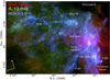 |
Fig. 1 Composite image of the ~5 deg2 area mapped in Orion B. Red color represents the PACS 70 μm emission tracing FUV-illuminated extended warm dust. Green color represents the cloud depth in magnitudes of visual extinction, AV ∝ N(H2). Blue color represents the HCN J = 1−0 line intensity. We note that outside the main filaments most of the HCN J =1−0 emission is at AV < 4 mag. |
Spectroscopic parameters of the lines studied in this work (from Endres et al. 2016, and references therein), critical densities for collisions with p-H2 and electrons at 20 K (if LTE prevails, 99.82% of H2 is in para form), and critical fractional abundance of electrons (see text).
Properties of the massive stars creating H II regions.
2 Observations
2.1 The Orion B GMC
Orion B, in the Orion complex, east of the Orion Belt stars, is one of the nearest GMCs (e.g., Anthony-Twarog 1982). Here we adopt a distance1 of d = 400 pc. Orion B is a good template to study the star formation processes in the disk of a normal galaxy. This is an active but modest star-forming region (with a low SFR ~ 1.6 × 10⁻⁴ M⊙ yr−1 and low star-formation efficiency, SFE ~ 1%, e.g., Lada et al. 2010; Megeath et al. 2016; Orkisz et al. 2019) that contains thousands of dense molecular cores: starless, prestellar, and protostellar cores (e.g., Könyves et al. 2020). Massive star formation is highly concentrated in four main regions: NGC 2071 and NGC 2068 in the northeast, and NGC 2023 and NGC 2024 in the southwest. Table 2 summarizes the properties of the massive stars that create H II regions in the field. Figure 2b shows the position and extent of these H II regions (marked with circles). Orion B hosts a complex network of filaments. The main and longest filaments are the Flame and Hummingbird filaments, Orion B9, and the Cloak (Orkisz et al. 2019; Gaudel et al. 2023). Appendix A outlines the main properties of these regions.
2.2 ORION-B molecular line maps in the 3 mm band and spatial smoothing
The ORION-B project (PIs: J. Pety and M. Gerin) is a large program that uses the 30m telescope of the Institut de Radioastronomie Millimétrique (IRAM) to map a large fraction of the Orion B molecular cloud (5 square-degrees, 18.1 × 13.7 pc2). Observations were obtained using the EMIR090 receiver at ~21″–28″ resolution. The FTS backend provided a channel spacing of 195 kHz (0.5–0.7 km s−1 depending on the line frequency). The typical 1σ line sensitivity in these maps is ~100 mK per velocity resolution channel. The full field of view was covered in about 850 h by (on-the-fly) mapping rectangular tiles with a position angle of 14° in the Equatorial J2000 frame that follows the global morphology of the cloud. Data reduction was carried out using GILDAS2/CLASS and CUBE. This includes gridding of individual spectra to produce regularly sampled maps, at a common angular resolution of 30″, with pixels of 9″ size, about one third of the angular resolution of the telescope (half power beam width, HPBW). The projection center of the maps is located on the Horsehead photodissociation region (PDR) at 5h40m54.27s, −02°28′00.0″. We rotated the maps counter-clockwise by 14° around this center. Pety et al. (2017) presents a detailed description of the observing procedure and data reduction. Here we focus on a global analysis of the HCN J = 1−0 emission, and its relation to that of HNC, 12CO, and HCO+. Orion B shows three main velocity components at the local standard of rest (LSR) velocities ~2.5, ~6, and ~10 km s−1 (Gaudel et al. 2023). Here we obtained the line intensity maps (zero-order moment maps) integrating each line spectrum in the velocity ranges [−5, +25] km s−1 (for 12CO and HCN J = 1−0 lines) and [0, +18] km s−1 (for HNC and HCO+ J =1−0). We refer to Gaudel et al. (2023) for a thorough analysis of the 13CO and C18O J = 1−0 maps and gas kinematics.
To match the resolution of the [C I] 492 GHz map (see next Section), and since we are interested in the faint and extended molecular emission, we spatially smoothed the original line maps to an angular resolution of ~2′ (~0.2pc). This allows us to recover a significant fraction of low surface brightness line emission at large spatial scales. Spatial smoothing improves the root mean square (rms) to ~25 mK per velocity channel. Thus, it improves the detection limit and signal-to-noise ratio (S/N) of the faint and extended emission. Figure 2 shows the spatially smoothed maps.
2.3 Wide-field [C I] 492 GHz map
We complement our molecular line maps with an existing wide-field map of the ground-state fine structure line (3P1−3P1) of neutral atomic carbon, the [C I] 492 GHz line, obtained with the Mount Fuji submillimeter-wave telescope. These observations reached a rms noise of ~0.45 K per 1.0 km s−1 velocity channel (Ikeda et al. 2002). The angular resolution is ~2′. Figure 2h shows the [C I] 492 GHz line integrated intensity map in the LSR velocity range [+3, +14] km s−1.
2.4 Pointed observations of rotationally excited lines
In addition to the molecular J =1−0 line maps, we observed several cloud positions (see Table 3 for the exact coordinates and details) in rotationally excited lines (J = 2−1, 3−2, and 4−3). We obtained these observations also with the IRAM-30m telescope. We observed 14 positions representative of different cloud environments: cold and dense cores, filaments and their surroundings, PDRs adjacent to H II regions and cloud environment. Figure 2 shows the location of these positions. We used the EMIR receivers E150 (at 2 mm), E230 (at 1.3 mm), and E330 (at 0.9 mm) in combination with the FTS backend (195 kHz spectral resolution). The HPBW varies as ≈2460/Freq[GHz]3. For the E1, E2, and E3 bands, the HPBW is ~14″, ~9″, and ~7″, respectively. We carried out dualband observations combining the E1 and E3 bands, during December 2021 and 2022, under excellent winter conditions (~1−4 mm of precipitable water vapor, pwv). We obtained the E2 band observations during three different sessions: (i) December 2021: pwv<4 mm (positions #1, #2, #4, #10, and #11), (ii) March 2022: pwv>6 mm (#3 and #7), (iii) May 2022: pwv ~ 5 mm ( #6, #8, #12, #13, and #14).
In order to compare line intensities at roughly the same 30″ resolution, we averaged small raster maps centered around each target position and approximately covering the area of a 30″ diameter disk (Fig. F.1 shows our pointing strategy). The total integration time per raster-map was ~1 h, including on and off integrations. The achieved rms noises of these observations, merging all observed positions of a given raster-map, are ~22 mK (J =2−1), ~20 mK (J = 3−2), and ~30 mK (J = 4−3), per 0.5 km s−1 velocity channel. Table F.1 summarizes the frequency ranges observed with each backend, the HPBW, and the number of pointings of each raster map.
We analyzed these pointed observations with CLASS. We subtracted baselines fitting line-free channels with first or second order polynomial functions. We converted the intensity scale from antenna temperature,  , to main-beam temperature, Tmb, as
  , where Feff and Beff are the forward and beam efficiencies3. Figure 3 shows a summary of the spectra. Figures G.1 and G.2 show the complete dataset.
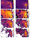 |
Fig. 2 Maps of Orion B in different tracers. (a) Visual extinction AV, (b) Approximate FUV field, |

Representative environments of our pointed observations.
2.5 Herschel Td, AV, and G′0 maps
In addition to the molecular and atomic line maps, we also make use of the dust temperature (Td) and 850 µm dust opacity (τ850 µm) maps fitted by Lombardi et al. (2014) on a combination of Planck and Herschel data from the Herschel Gould Belt Survey (HGBS) (André et al. 2010). In Appendix C we provide additional details on these maps. We estimated the (line of sight) visual extinction from the τ850 µm dust opacity map following Pety et al. (2017):
![${A_{\rm{V}}} = 2.7 \times {10^4}\,{\tau _{850\,\,{\rm{\mu m}}}}\,\left[ {{\rm{mag}}} \right].$](/articles/aa/full_html/2023/11/aa46598-23/aa46598-23-eq13.png) (1)
(1)
By taking the τ850 µm error map of Lombardi et al. (2014), we determine that the mean 5cr error of the AV map is about 0.8 mag.
This value is slightly above our molecular line detection threshold (AV ≃ 0.3–0.4 mag, see Fig. 4). Thus, we caution that one can probably not trust any AV−W trend below AV ≃ 0.8 mag. For each line of sight, we determined the FIR surface brightness, IFIR, from spectral energy distributions (SED) fits, by integrating:
![${I_{{\rm{FIR}}}} = \,\int {{I_v}\,dv} = \int {{B_v}} \left( {{T_{\rm{d}}}} \right)\left[ {1 - {{\rm{e}}^{ - {\tau _v}}}} \right]\,\,dv,$](/articles/aa/full_html/2023/11/aa46598-23/aa46598-23-eq14.png) (2)
(2)
from λ = 40 to 500 µm. In this expression, Bv(Td) is the blackbody function,  is the frequency-dependent dust opacity (we adopt the same emissivity exponent as Lombardi et al. 2014), and Td is an effective dust temperature.
We estimate the strength of the far-UV (FUV) radiation field (6 < E < 13.6 eV), in Habing units (G′0), from IFIR using:
![$G{\prime _0} = {1 \over 2}{{{I_{{\rm{FIR}}}}\,\left[ {{\rm{erg}}\,{{\rm{s}}^{ - 1}}\,{\rm{c}}{{\rm{m}}^{ - 2}}\,{\rm{s}}{{\rm{r}}^{ - 1}}} \right]} \over {1.3 \times {{10}^{ - 4}}}}.$](/articles/aa/full_html/2023/11/aa46598-23/aa46598-23-eq16.png) (3)
(3)
In this expression we assume that the FIR continuum emission arises from dust grains heated by stellar FUV and visible photons (Hollenbach & Tielens 1999). We use the notation G′0 (meaning approximate G0) because this expression is precise for a face-on PDR (e.g., it is valid for NGC 2024 and NGC 2023). Because of their edge-on geometry, Eq. (3) is less accurate for the Horse-head PDR and IC 434 front (although it provides the expected G0 within factors of a few). In addition, Eq. (3) provides an upper limit to the actual G0 toward embedded star-forming cores (at high AV). These cores emit significant non-PDR FIR dust continuum. To directly compare our line emission maps with the AV, G′0, and IFIR maps, we also spatially smoothed these SED-derived maps to an angular resolution of 120″ (Figs. 2a and b).
3 Results
3.1 Spatial distribution of the HCN J = 1−0 emission, relation to other chemical species, and AV and G′0 maps
Figure 1 shows a composite RGB image of the mapped area (~ 5deg2 = 250 pc2). This image shows extended HCN J = 1−0 emission far from the main dense gas filaments (where AV > 8 mag), as well as very extended 70 µm dust emission (e.g., André et al. 2010) from FUV-illuminated warm grains. Figure 2 shows the spatial distribution of the12 CO, HCO+, HCN, and HNC J = 1-0 integrated line intensities, W (also dubbed line surface brightness) at a common resolution of ~2′ (~0.2 pc, thus matching the angular resolution of the [C I] 492 GHz map in Fig. 2g). W(HCN J = 1−0) refers the sum of the three HFS components. The emission from all species peaks toward NGC 2024. The last column in Table 4 shows that spatial smoothing (increasing the line sensitivity at the expense of lower spatial resolution) allows us to detect HCN and HNC J = 1−0 emission from a cloud area nearly four times bigger than from maps at ~30″ resolution. For CO J = 1−0 (very extended emission) the recovered area is smaller. CO J = 1−0 shows the most widespread emission. It traces the most extended and translucent gas, arising from 90% of the mapped area. HCO+ and HCN J = 1−0 are the next molecular lines showing the most extended distribution, 73% and 60% of the total observed area, respectively. On the other hand, HNC J = 1−0 shows a similar distribution as C18 O J = 1−0 (Gaudel et al. 2023).
Table 4 provides the total line luminosity (LLine) from the mapped area in L⊙ units. LLine is the power emitted through a given line. It also provides  (in units of K km s−1 pc2), with:
 (4)
(4)
where Ω is the solid angle subtended by the source area and Waverage is the average spectrum over the mapped area A. This last quantity is commonly used to express mass conversion factors (see Sect. 6.3) and it is also frequently used in the extra-galactic context (e.g., Gao & Solomon 2004a; Carilli & Walter 2013). The 12CO J = 1−0 luminosity over the mapped area, ~1.7 L⊙ is more than a hundred times higher than  and LHCN 1−0.
Figures 2a and b show maps of visual extinction (AV) and the approximate strength of the FUV radiation field G′0 (see Sect. 2.5). Table 5 summarizes the median, average, and standard deviation values of the SED-derived parameters. The star-forming cores at the center of the NGC 2024 have the highest AV values, with a secondary peak toward NGC 2023 star-forming cores. The highest values of G′0 correspond to cloud areas in the vicinity of the HII regions NGC 2024 (G′0 ≈ 104), with a contribution from the neighbor H II region created by Alnitak star (G′0 ≈ 103), NGC 2023 (G′0 ≈ 103), IC 435 (G′0 ≈ 102), and the ionization front IC 434 (G′0 ≈ a few 102) that includes the iconic Horsehead Nebula. On the other hand, the easter part of the cloud shows low surface brightness IFIR emission compatible with G′0 of a few to ≃ 10. The median G′0 in the mapped region is 9.
Figure 4 shows 2D histograms of the CO, HCN, HCO+, HNC J =1−0, and [C I] 492 GHz integrated line intensities as function of the visual extinction into the cloud4. The running median of the HCN J =1−0 emission increases with extinction at AV > 3 mag, whereas the running median of the HNC J =1−0 emission shows a similar change of tendency but at higher extinction depths AV > 5 mag. As HCN, the largest number of HCO+ J =1−0 and [C I] 492 GHz line detections in the map occur at AV ≃ 3 mag. Atomic carbon, however, shows an approximate bimodal behavior with AV (it shows both bright and faint emission at high Ay). Indeed, while AV is the total visual extinction along each line of sight, we expect that in many instances the [C I] 492 GHz emission mostly arises from cloud rims close to the C0/CO transition (e.g., Hollenbach et al. 1991). On the other hand, lines of sight of large AV and very bright [C I] 492 GHz emission (such as NGC 2024) probably trace FUV-illuminated surfaces of multiple dense cores and PDRs along the line of sight.
Following Pety et al. (2017), Fig. 5a shows the fraction of total Lline within a set of four visual extinction masks. The mask with AV>15 mag (~1% of the total mapped area) represents the highest density gas associated with dense cores. The mask within the AV range 8–15 mag (~ 3% of the mapped area) is right above the extinction threshold above which the vast majority of prestellar cores are found in molecular clouds (e.g., Lada 1992; Lada et al. 2010; Wu et al. 2010; Evans et al. 2020). Below this threshold, we create two masks to differentiate the emission associated with AV below 4 mag (translucent and PDR gas; ~80% of the mapped area) and 4 < AV < 8 mag (intermediate cloud depths representing ~16% of the mapped area). We find that more than half of the total CO J = 1−0 intensity arises from the lowest extinction mask AV<4 mag. Interestingly, about a 30% of the total HCN J = 1−0 emission arises from gas also at AV<4 mag. Most of the HCN and HNC J = 1−0 emission arises from regions at visual extinctions between 4 and 8 mag, and only 10% of the HCN emission arises from regions at very high visual extinctions, AV > 15 mag. Likewise, the HCN and HNC 2D histograms peak at AV lower than 3 mag (HCN) and 5 mag (HNC). This contrasts with the N2H+ J = 1−0 emission, which arises from cold and dense gas shielded from FUV radiation at AV > 15 mag (see Pety et al. 2017). For each molecular line, Fig. 5b shows the typical (the statistical mode) intensity W toward each of the four extinction masks. The CO J = 1−0 emission is bright (~1 K km s−1) even at AV < 4 mag, and very bright (> 10 K km s−1) toward all the other masks (although optically thick).
The typical HCN, HNC, and HCO+ J = 1−0 line intensities are above 1 K km s−1 for AV > 15 mag (dense gas). For lower AV, the lines are fainter but detectable. Since the translucent gas spans much larger areas than the dense gas (96% of the mapped cloud is AV < 8 mag, 80% at AV < 3 mag), in many instances it is the widespread and faint extended emission that dominates the total luminosity. We stress that -70% of the HCN J = 1−0 line luminosity in Orion B arises from gas at AV < 8 mag (and 50% of the FIR dust luminosity). Table 4 summarizes the line intensities and line luminosities over the mapped area.
Figure 5c shows the cumulative fractions of the integrated intensities for CO, HCO+, HCN, HNC J =1−0 as a function of AV. The cumulative distributions are different for each species. We define the visual extinction that contains 50% of the total integrated line intensity as the characteristic AV, such as  (e.g., Barnes et al. 2020). We find that the characteristic
  for CO J = 1−0 is 3.8 mag, which implies that 50% of the CO total intensity arises from gas below AV = 3.8 mag. For HCO+, HCN, and HNC J = 1−0 lines, we find
  of 5.0, 5.8, and 6.7 mag, respectively. These values agree with recent studies of the star-forming regions Orion A and W49 (Kauffmann et al. 2017; Barnes et al. 2020).
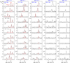 |
Fig. 3 Selection of HCN J = 1−0 to 4−3, and HNC J = 3−2 line detections toward representative cloud environments in OrionB. Red lines show the expected relative HFS line intensities in the LTE and optically thin limit. |
Characteristics of the molecular line emission over 5 deg2 of Orion B.
SED derived parameters from 5 deg2 maps of Orion B.
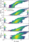 |
Fig. 4 Distribution of 12CO, HCN, HCO+, HNC J = 1−0, and [C I] 492 GHz line intensities as a function of AV. The dashed red lines show the running median (median values of the line intensity within equally spaced log AV bins). Error bars show the line intensity dispersion. We note that the 5σ error of AV is ≃0.8 mag. Thus, one cannot trust any trend below this threshold. |
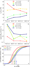 |
Fig. 5 Line emission properties as a function of AV. (a) Fractions (in %) of line luminosities emitted in each Ay mask. (b) Typical (the mode) line intensity in each AV mask. (c) Cumulative line luminosity. |
3.2 HCN/CO, HCN/HNC, HCN/HCO+, and [C I]/CO line intensity ratio maps
The spatial distribution of the HCN J = 1−0 line emission compared to that of other molecules provides information about the origin and the physical conditions of the HCN-emitting gas. Figure 6 shows the HCN/12 CO J = 1−0, HCN/HNC J = 1−0, and HCN/HCO+ J = 1−0 integrated line intensity ratios. We generated these maps by taking only line signals above 3σ for each species (i.e., we show regions where the emission from both species spatially coexist along the line of sight). In addition, Fig. 6d shows a map of the [C I] 492 GHz/CO J = 1−0 integrated line intensity ratio5). Table 6 summarizes the average and median line intensity ratios in the mapped region.
HCN/CO J = 1−0: The average line intensity ratio is 0.015, with a standard deviation of 0.023. In the inner regions of the cloud, close to the Cloak, Orion B9, Hummingbird, and Flame filaments, the ratio increases with AV (shown in contours). We also find high line intensity ratios (~0.1) in the FUV-illuminated cloud edges (see discussion in Sect. 6.2).
HCN/HNC J = 1−0: The average line intensity ratio is 3.1, with a standard deviation of 1.2. The lowest ratios, ~0.5–0.9, appear in cold and low IFIR regions such as the Cloak and Orion B9.
HCN/HCO+ J = 1−0: The average line intensity ratio is 0.9, with a standard deviation of 0.4. In general, this line ratio displays small variations across the cloud. The Cloak, the center of NGC 2024, the Flame Filament, and the Horsehead show a line intensity ratio above one (reddish areas in Fig. 6c). All these regions host starless and prestellar cores (Könyves et al. 2020).
[C I] 492 GHz/CO J = 1−0: The average line intensity ratio is 0.20, with a standard deviation of 0.26. In PDR gas, this ratio is roughly inversely proportional to the gas density (see e.g., Kaufman et al. 1999). We find the highest ratios, above one, toward the FUV-illuminated edges of the cloud.
We also investigate the possible spatial correlations of the above line intensity ratios with the SED derived parameters G′0, Td, Tpeak(CO), and Av. Only the HCN/HNC J = 1−0 line intensity map shows a (weak) monotonic correlation with G′0 (Spearman correlation rank of 0.6; see Table 6). This spatial correlation is not linear (the Pearson correlation rank is 0.5 in log-log scale and 0.008 in linear scale) but suggests a connection between the HCN/HNC abundance ratio and the FUV radiation field. Figures B.1 and Fig. B.2 show 2D histograms of the studied line intensity ratios as function a of AV and IFIR, respectively.
4 HCN excitation, radiative transfer models, and gas physical conditions
In this section we analyze the large scale HCN J = 1−0 emission in detail. We, (i) derive excitation temperatures (Tex) and HCN column densities, N(HCN), using the LTE-HFS fitting method, (ii) analyze the anomalous HCN J = 1−0 HFS emission, (iii) determine the physical conditions of the widespread and extended HCN J = 1−0 emitting gas, and (iv) derive rotational temperatures, Trot, and N(HCN) in a sample of representative positions observed in rotationally excited HCN and H13CN lines. In order to determine all these parameters at the highest possible spatial resolution, throughout all this section we make use of maps and pointed observations at an effective 30″ resolution (~0.06 pc).
4.1 HCN column density and Tex using the LTE-HFS method
Firstly, we determine Tex (J = 1−0) and the opacity-corrected column density Nτ,corr(HCN) by applying the LTE-HFS fitting method in CLASS2 (Appendix D.1). This method uses as input the line separations and 1:5:3 intrinsic line strengths of the J =1−0 HFS components. The LTE-HFS fitting method assumes that: (i) all HFS lines have the same Tex and linewidth Δυ, and (ii) the velocity-dependent line opacities have Gaussian profiles. Thus, one can express the continuum-substracted main beam temperature at a given velocity υ of the J =1−0 line profile as:
![${T_{{\rm{mb}}}}\left( \upsilon \right) = \left[ {J\left( {{T_{{\rm{ex}}}}} \right) - J\left( {{T_{{\rm{bg}}}}} \right)} \right]\,\,\left[ {1 - {{\rm{e}}^{ - \tau \left( \upsilon \right)}}} \right],$](/articles/aa/full_html/2023/11/aa46598-23/aa46598-23-eq25.png) (5)
(5)
where τ(υ) is the sum of the HFS line opacities:
 (6)
(6)
In the above expressions,  is the opacity of each HFS component i at (each) line center (
 ), and
  is a Gaussian profile centered at
  . In the LTE-FTS fitting method, one fixes the sum of all HCN J =1−0 HFS line center opacities, τ0, following their intrinsic line strengths:
 (7)
(7)
In the Rayleigh-Jeans regime, J(Tex) → Tex. Thus, the LTE-HFS fitting method returns Tex and τ0 as outputs. We use these parameters to derive Nτ,corr (HCN). In order to obtain satisfactory fits, we applied this method to the brightest regions, those  (HCN J =1−0 F = 2−1, ≥0.5 K = 5σ), associated with the main cloud velocity component at υLSR ≃10 km s−1.
Figure 7 shows the resulting HCN column density and Tex maps in a smaller but high S/N submap. The average (median) Tex (J = 1−0) in the region is 5 K (4.5 K), implying subthermal emission, that is, Tex ≪ Tk and n(H2) < ncr, eff. NGC 2024 shows the highest values, with Tex > 15 K. Nτ,corr(HCN) ranges between 1013 and a few 1014 cm−2. The average (median) column is 3.4×1013 cm−2 (1.3×1013 cm−2).
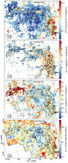 |
Fig. 6 Line intensity ratio maps. Contours show AV = 4, 6, 8, and 15 mag. |
4.2 Large-scale anomalous HCN J = 1−0 HFS emission
To study the HCN J = 1−0 emission in more detail we extracted the intensity and linewidth of each HFS component individually (by fitting Gaussians). Figures 7c and d show the spatial distribution of the HFS line intensity ratios, R02 = W(F = 0–1)/W( F = 2−1) and R12 = W(F = 1–1)/W(F = 2−1), respectively, and Fig. 8a shows their histograms. In addition, Fig. 8b shows the histograms of the HFS linewidth ratios,  and
and  . The red curve in Fig. 8a shows the expected R02 and R12 ratios in LTE as line opacities increase. We note that the majority of observed ratios in the map are far from the LTE curve. Indeed, the histogram of the intensity ratio R02 peaks at 0.21, with a median value of 0.25 whereas the histogram of the intensity ratio R12 peaks at 0.52, with a median value of 0.56. Therefore, the intensity ratio R12 is typically anomalous6 over large cloud scales.
Non-LTE radiative transfer models including line overlap effects show that these anomalous intensity ratios imply that lines are optically thick and that a single Tex does not represent the excitation of these HFS levels (Gonzalez-Alfonso & Cernicharo 1993; Goicoechea et al. 2022). This questions the precision of the parameters obtained from the LTE-HFS fitting method. To illustrate this, Fig. D.1 shows the (poor) best LTE-HFS fit to the HCN J = 1−0 HFS lines toward the Horsehead PDR.
The linewidth of the faintest F = 0−1 HFS component in the map ranges from ~1 to ~2 k m s−1 (see also Table G.1). These linewidths are broader than the narrow linewidths, ~0.5 km s−1, typically observed in Orion B toward dense and FUV-shielded cold cores in molecules such as H13CO+ (e.g., Gerin et al. 2009). Thus, HCN J = 1−0 traces a different cloud component. Figure 8b shows the histogram of the HFS linewidth ratios  and
and  . They peak at 0.75 and 0.91 respectively, with median values of 0.91 and 1.03. That is, the linewidths of the different HFS components are not the same and line opacity broadening matters. Non-LTE models including line overlap predict these anomalous linewidth ratios, RΔυ≠1, when HFS lines become optically thick (e.g., see Fig. 3 of Goicoechea et al. 2022).
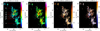 |
Fig. 7 Spatial distribution of Tex(HCN J = 1−0) and N(HCN) estimated from LTE-HFS fits, and maps of HCN J = 1−0 HFS intensity ratios. (a) Tex(HCN J = 1−0). (b) Opacity-corrected column densities N(HCN). (c) and (d) R02 and R12 (white color corresponds to non-anomalous ratios). |
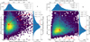 |
Fig. 8 Histograms of HCN J =1−0 HFS (a) Line intensity ratios, and (b) Line-width ratios observed in OrionB. R02 stands for W(F = 0−1)/W(F = 2−1) and R12 stands for W(F = 1–1)/W(F = 2−1). The red curve in panel (a) shows the expected LTE ratios as line opacities increase. The red star marks the non-anomalous ratios in the optically thin limit τ → 0 (1σ is the standard deviation relative to the mean line ratios). |
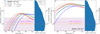 |
Fig. 9 Comparison of observed W(HCN J = 1−0) intensities in Orion B and predictions from nonlocal and non-LTE radiative transfer models including line overlap for (a) N(HCN) = 1013 cm−2 and (b) N(HCN) = 1014 cm−2. The continuous curves show model results for Tk = 60, 30, and 10 K (red, green, and blue curves, respectively), different ionization fractions: χe = 0 (continuous curves), χe = 2×10⁻⁵ (dashed curves), and χe = 10−4 (dotted curves). The pink and orange horizontal line mark the mean and median values of W(HCN J = 1−0). The pink shaded area represents the standard deviation (1er) relative to the mean detected W(HCN J = 1−0) intensities in Orion B (at 30″). Positions in the pink area account for -70% of the total LHCN 1−0 in the map. The right panels show an histogram with the distribution of W(HCN J =1−0) detections in individual map pixels. |
4.3 Physical conditions of the extended low surface brightness HCN J = 1−0 emitting gas
Here we compare the observed line integrated intensities W(HCN J = 1−0) with a grid of non-local and non-LTE radiative transfer models calculated by Goicoechea et al. (2022). These models include HFS line overlaps and use new HFS-resolved collisional rate coefficients for inelastic collisions of HCN with para-H2, ortho-H2, and electrons in warm gas.
The grid of single-component (Tk = 60, 30, and 10 K) static-cloud (no velocity field) models encompass the HCN column densities predicted by our chemical models (Sect. 5) and typically observed in Orion B (Fig. 7b): N(HCN)= 1013 cm−2, representative of optically thin or marginally optically thick HCN J = 1−0 HFS lines, and N(HCN) = 1014 cm−2, representative of bright optically thick lines. The range in gas densities n(H2) goes from ~107 cm−3, only relevant to hot cores and protostellar envelopes, to nearly 102 cm−3, relevant to the most extended and FUV-illuminated component of GMCs. As we are mostly interested in this component, these models compute the HCN excitation for three different electron abundances: χe = 10−4, 2 × 10⁻⁵, and 0. Figure 9 shows model results (continuous curves) in the form of predicted line intensities W(HCN J = 1−0) as a function of n(H2).
The right panels in Fig. 9 show histograms with the distribution of W(HCN J = 1−0) detections (> 3σ) in individual pixels of the map. The mean (median) intensity7 in these pixels is 1.4 K km s−1 (0.97 K km s−1). The pink shaded area in Fig. 9 represents the 1σ dispersion relative to the mean W(HCN J = 1−0) value. However, while about 70% of the observed intensities have a value below the mean, less than 1% of the observed intensities have a value above 10 K km s−1 (very bright HCN emission). In the following we take W(HCN J = 1−0) = 1 K km s−1 as the reference7 for the extended cloud emission. Models with N(HCN) = 1013 cm−2 (Fig. 9a) encompass this W(HCN J = 1−0) intensity level. The gas temperature in this cloud component is Tk ≃ 30 to 60 K (translucent gas and UV-illuminated cloud edges; see specific PDR models in Sect. 5). Using N(HCN) = 1013 cm−2 and neglecting electron collisional excitation (χe = 0) we determine an upper limit to the gas density of n(H2) ≃ (1–3) × 104 cm−3.
Figure 10 shows the effect of electron excitation predicted by radiative transfer models appropriate to this extended and translucent gas (adopting n(H2) = 5 × 103 cm−3). The plot shows how W(HCN J = 1−0) (red curves) and Tex(HCN J = 1−0 F = 2−1) (blue curves) increase as the electron abundance χe increases. The reference intensity value, W(HCN J = 1−0) = 1 K km s−1, intersects the model curves at an electron abundance of a few 10−5 and Tex ≃ 3.2–3.5 K. These low excitation temperatures imply weak collisional excitation, but still Tex > TCMB.
Interestingly, the extended HCN J= 1−0 emission observa-tionally correlates well with the [C I] 492 GHz emission (see Fig. 2 and Sect. 6.2.1). In addition, our photochemical models show that χe reaches ≳ 10−5 in the [C I] 492 GHz emitting cloud layers (see Sect. 5). For such high χe values, electron excitation enhances the HCN J =1−0 emission at low gas densities (see Fig. 10 and Goldsmith & Kauffmann 2017; Goicoechea et al. 2022). Hence, we estimate that the median gas density in the extended cloud component is n(H2) ≃ (4–7) x 103 cm−3 if χe ≃ 2 × 10⁻⁵ (or ≃ 103 cm−3 if χe ≃ 10−4).
On the other hand, the strongest HCN-emitting regions in OrionB, those with W(HCN J = 1−0)>6 K km s−1, only represent ~15% of the total HCN J = 1−0 luminosity in the map. This bright HCN emission can only be reproduced by models with N(HCN) = 1014 cm−2 and higher gas densities, n(H2) > 105 cm−3.
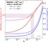 |
Fig. 10 W(HCN J = 1−0) (red curves) and Tex (HCN J = 1−0 F = 2−1) (blue curves) predicted by non-LTE radiative transfer models, appropriate to extended and translucent gas, as a function of electron abundance. The vertical pink shaded area intersects the typical W(HCN J = 1−0) = 1 K km s−1 intensity level ( ± 20%). |
4.4 Rotationally excited HCN and H13 CN toward representative cloud environments in Orion B
To complement our analysis of the HCN J = 1−0 emission at large spatial scales, and to determine more accurate HCN column densities, here we analyze our multiple- J HCN and H13CN line observations toward 14 positions in Orion B (see Table 3 for a brief explanation). Figure 3 shows a selection of the spectra. We detect HCN J = 2−1 and J=3−2 toward all positions, and HCN J = 4−3 toward five of the 14 observed positions (Fig. G.1 shows the spectra of all observed positions).
The HCN J =2−1 transition has six HFS lines that, for the narrow line widths in Orion B, blend into three lines with apparent relative intensity ratios ~ 1:9:2 in the LTE and optically thin limit (red vertical lines in Fig. 3). The HCN J =3−2 transition also has six HFS lines. Only the central ones are blended and cannot be spectrally resolved. This gives the impression of three lines with relative intensity ratios 1:25:1 in the LTE and optically thin limit (e.g., Ahrens et al. 2002; Loughnane et al. 2012). We term these three apparent components (blueshifted, central, and redshifted) of the J=2−1 and J=3−2 rotational lines as “satellite (B),” “main,” and “satellite (R),” respectively. We recall that these overlapping lines in the HCN J = 2−1 and 3−2 transitions are responsible of the observed anomalous HCN J = 1−0 HFS line intensity ratios (Goicoechea et al. 2022, and references therein).
Blue and red curves in Fig. 11 show the expected HCN J = 2−1 and J = 3−2 HFS intensity ratios satellite (R)/main versus satellite (B)/main in LTE as line opacities increase. Only when τ2−1 → 0 and τ3−2 → 0, one should detect the ~ 1:9:2 and ~1:25:1 HFS ratios. The filled dots in Fig. 11 show the observed ratios (summarized in Table D.1) toward the sample of representative positions that could be fitted with three Gaussian lines. This plot shows that several HCN J = 2−1, and specially J = 3−2, HFS line intensity ratios do not lie on the LTE curves even for elevated line opacities. That is, the emission of rotationally excited HCN lines can also be anomalous.
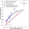 |
Fig. 11 HCN J = 2−1 and J = 3−2 HFS intensity ratios satellite(R)/main versus satellite(B)/main (see Sect. 4.4 for their definition) in LTE and as line opacities increase. Blue and red dots show the observed HFS line ratios toward the representative positions (see Table D.1). |
4.4.1 HCN and HNC rotational diagrams
Here we estimate the degree of excitation (by determining rotational temperatures, Trot) and column densities of HCN and HNC toward the sample of representative positions. We analyze the detected rotationally excited HCN (up to J = 4−3) and HNC (up to J = 3−2) lines by constructing rotational population diagrams in Appendix E (Goldsmith & Langer 1999). We derive N(HCN), and N(HNC) ignoring their HFS structure (i.e., only the total line intensity of each rotational transition matters).
This is a valid approximation to obtain Trot from observations of multiple-J lines. We derive the HCN column density and rotational temperature under the assumption of optically thin emission (Nthin and  ). We also determine their opacity-corrected values (Nτ,corr and
  ) by using the H13CN line intensities (see Fig. G.1) and assuming that the emission from HCN and H13CN lines arise from the same gas. Except for the brightest position #1, the derived HCN rotational temperatures range from 4 to 10 K (i.e. subthermal excitation), and NτcoII(HCN) ranges from 5 × 10¹² to 3.4× 1013 cm−2. Table summarizes the derived values and Appendix E shows the resulting rotational diagram plots. We employ the same methodology for HNC and HN13C. Rotational temperatures are also low, from 5 to 11 K. HNC column densities range from ~1012 to 1.6 × 1013 cm−2 (see Table E.1).
4.4.2 Comparison with single-component non-LTE models
Most of the observed representative positions likely have velocity, temperature, and density gradients (specially prestellar cores and protostars). However, carrying out a complete, source-by-source, radiative transfer analysis is beyond the scope of this study (more focused on the extended cloud component). Here we just used the outputs of the grid of single-component and static models computed by Goicoechea et al. (2022), and presented in Sect. 4.3, to estimate the physical conditions (gas temperature and densities) compatible by the detected rotationally excited HCN line emission. We compared the observed line intensity ratios  and
and  summarized in Table 7 with the models shown in Fig. 10 of Goicoechea et al. (2022). As an example, the observed line ratios toward the Horsehead PDR are
  and
and  . These ratios can be explained by models with Tk = 30–60 K and n(H2) of a few 104 cm−3. Position #14 shows the lowest line ratios of the sample,
  and
and  , which is consistent with n(H2) of a few 104 cm−3. On the other hand, the observed line intensity ratios toward position #1 (center of NGC 2024) are
  and
and  . In this position we derive the highest HCN rotational temperature (~38 ± 10 K). The observed
  intensity ratios are consistent with the presence of dense gas, n(H2) ≥ 106 cm−3.
4.5 HCN/HNC intensity and column density ratios
Table 8 summarizes the resulting N(HCN)/N(HNC) column density ratios obtained from rotational population diagrams (Sect. 4.4.1) as well as W(HCN)/W(HNC) J = 1−0 and J =3−2 line intensity ratios. The positions that host lower excitation conditions (e.g., low Trot(HNC)) tend to have lower N(HCN)/N(HNC) column and W(HCN)/W(HNC) intensity ratios. Mildly FUV-illuminated environments such as the Horsehead nebula show W(HCN)/W(HNC) line intensity ratios of about two, whereas the most FUV-shielded cold cores and their surroundings (positions #7, #8, #10, #13) display ratios of about one. On the other hand, the most FUV-irradiated and densest cloud environments (those with HCN J= 4−3 detections in NGC 2024) show ratios of at least four (positions #1 and #2).
These results roughly agree with the spatial correlation between the HCN/HNC J = 1−0 integrated line intensity ratio and G0 in the entire region. Figure 12 shows a 2D histogram of the observed W(HCN)/W(HNC) J =1−0 intensity ratio as a function of G′0 in the mapped region. The running median HCN/HNC J = 1−0 intensity ratio increases from ≃ 1 at G′0 ≃10 to ≃3 at G′0 ≃200. For higher values of G′0, the running median intensity ratio stays roughly constant at ≃ 3–4. We estimate that the higher HCN J = 1–0 line opacity toward these bright positions (at least τ ≃ 5-10, see Table D.1) compared to that of HNC J = 1–0 (on the order of τ ≃ 1–3, Table E.1) contributes to the observed constancy of the line intensity ratio.
In FUV-illuminated environments, the strength of the radiation field influences the gas chemistry and determines much of the gas temperature and electron abundance (see Sect. 5). At a given abundance, HNC responds more weakly to electron excitation than HCN. In particular, the HCN J =1–0 critical fractional abundance of electrons ( in Table 1) is a factor of ~4 lower than that of HNC J =1–0. Moreover, HNC is typically less abundant in FUV-illuminated gas (Sect. 5).
In addition, as HCN and HNC rotational lines become optically thick, HFS line overlap effects become important for both species. However, their relative effect as a function of J are different (Daniel & Cernicharo 2008). These aspects ultimately drive their excitation and contribute to the slightly different rotational temperatures we infer for the two species. Still, modeling the HFS resolved excitation of HNC is beyond the scope of our study. Future determinations of HFS-resolved HNC-H2 inelastic collision rate coefficients will make such detailed studies feasible.
HCN J = 1−0 HFS line intensity ratios, W(HCN J = 2−1)/W(HCN J =1−0) and W(HCN J = 3−2)/W(HCN J =1−0) line intensity ratios, and parameters derived from rotational population diagrams, computed in Appendix E, toward a sample of representative cloud positions.
HNC rotational temperatures, HCN/HNC column density, and line intensity ratios toward selected positions in Orion B.
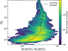 |
Fig. 12 2D histogram of the observed HCN/HNC J = 1–0 line intensity ratio as a function of G′0 in the Orion B map. The dashed black curve shows the running median. The error bars show the standard deviation. |
5 HCN and HNC chemistry in FUV-illuminated gas
To guide our interpretation of the extended HCN J =1–0 emission, here we reassess the chemistry of HCN, HNC, and related species in FUV-illuminated gas. The presence of FUV photons, C+ ions, C atoms, and high electron abundances triggers a distinctive nitrogen chemistry, different to that prevailing in cold and dense cores (e.g., Hily-Blant et al. 2010) shielded from FUV radiation. Sternberg & Dalgarno (1995), Young Owl et al. (2000) and Boger & Sternberg (2005) previously studied the formation and destruction of HCN in FUV-irradiated gas. Here we used an updated version of the Meudon PDR code (Le Petit et al. 2006) that implements a detailed treatment of the penetration of FUV photons (Goicoechea & Le Bourlot 2007) and includes v-state-dependent reactions of FUV-pumped H2(υ) (hereafter  ) with neutral N atoms leading to NH + H (Goicoechea & Roncero 2022), as well as reactions of o-H2 and p-H2 with N+ ions, leading to NH+ + H (Zymak et al. 2013).
We also included the isomerization reaction:
 (8)
(8)
with a rate coefficient k(T) = 10−10 exp(−Eb/T), where Eb is the reaction energy barrier. Theoretical calculations agree on the presence of a barrier, however, different methods provide slightly different barrier heights: ~2130K (Talbi et al. 1996), ~1670K (Sumathi & Nguyen 1998), and ~960K (Petrie 2002). In our models we initially adopt Eb = 1200 K (see Graninger et al. 2014). We also included the isomerization reaction:
 (9)
(9)
which is generally not included in dark cloud chemical models but plays a role in FUV-illuminated gas. We adopt a rate coefficient k(T) = 1.6 × l·0−10 cm3 s−1 and no energy barrier (from calculations by Loison et al. 2014; Loison & Hickson 2015).
In order to accurately treat the photochemistry of HCN and HNC, our models explicitly integrate their photodissociation and photoionization cross sections at each cloud depth. We use the wavelength-dependent cross sections tabulated in Heays et al. (2017), which include a theoretical calculation of the HNC photodissociation cross section by Aguado et al. (2017). For the interstellar radiation field, this cross section implies that HNC is photodissociated about two times faster than HCN.
We adopted a H2 cosmic ray ionization rate ζCR of 10−16 s−1, typical of translucent gas and cloud edges in the disk of the galaxy (e.g., Indriolo et al. 2015). We assumed standard interstellar dust grain properties and extinction laws. We ran photochemical models adapted to the illumination conditions and gas densities at large scales in Orion B. In particular, we adopted a representative FUV field of G0 = 100, typical of the Horsehead edge, the IC 434 ionization front, and close to the mean G0 in the mapped area (see Table 5). Nonetheless, we note that adopting lower G0 values basically shifts the abundance profiles to lower cloud depths but the following chemical discussion remains very similar. Figure 13 shows the predictions of constant density models, with nH = 5 × 103 cm−3 (left panels) and nH = 5 × 104 cm−3 (right panels). Figures 13a and b show the predicted column density ratios (upper panels) and abundance8 profiles (lower panels) as a function of cloud depth, in mag of visual extinction9.
We determine molecular column densities at a given cloud depth AV (or cloud path length l) by integrating the predicted depth-dependent abundance profile, x(species), from 0 to AV:
 (10)
(10)
where x(l) is the species abundance, with respect to H nuclei7, at a cloud path length l.
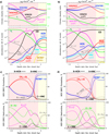 |
Fig. 13 Constant density gas-phase PDR models with G0 = 100 and nH = 5 × 103 cm−3 (left) and 5 × 104 cm−3 (right). These models adopt Eb = 1200 K for Reaction (8). Upper panels in (a) and (b): dashed curves show the depth-dependent column density ratios of selected species (left y-axis). The blue continuous curves in the upper panels of (a) and (b) show the HCN/HNC column density ratio adopting Eb = 200 K. Green continuous curves show the temperature structure as a function of AV (right y-axis). Lower panels in (a) and (b): abundance profiles with respect to H nuclei. (c) and (d): Contribution (in percent) of the main formation and destruction reactions for HCN (continuous curves) and HNC (dashed curves). |
5.1 Chemistry at cloud edges, AV < 4 mag
The red shaded areas in Fig. 13 show model results for AV < 4 mag typical of FUV-illuminated cloud edges. FUV photons drive the chemistry in these translucent layers that host the C+ to C transition and have high electron abundances: from xe ≃ x(C+) ≃ 10−4 to xe ≃ 10−6 depending on AV and G0/nH. To simplify our chemical discussion, Fig. 14 summarizes the network of dominant chemical reactions at AV < 4 mag. Wherever C+ is abundant, reactions of CH2 with N atoms dominate the formation of HCN and HNC, as shown by the red curves in Figs. 13c and 13d. These two figures show the contribution (in percent) of the main HCN and HNC formation and destruction reactions as a function of cloud depth. The second most important path for HCN and HNC formation at AV < 4 mag is HCNH+ dissociative recombination. HCN and HNC destruction is governed by photodissociation and by reactions with C+. Their exact contribution depends on the gas density and G0. Our model assumes that the rate coefficient of reactions C+ + HCN and C+ + HNC, as well as the branching ratios of dissociative recombination HCNH+ + e → HCN/HNC + H, are identical for both isomers (e.g., Semaniak et al. 2001). Therefore, the N(HCN)/N(HNC) column density ratio at AV < 4 mag basically depends on the differences between HCN and HNC photodissociation cross sections. Wherever photodissociation dominates (e.g., green curves in Figs. 13c and 13d), we predict N(HCN)/N(HNC) ≃ 1.5–2.5. These values are consistent with the ratio inferred toward the rim of the Horsehead, a nearly edge-on PDR (see Table 8).
Neutral atomic carbon reaches its abundance peak at AV ≃1–3 mag (depending on nH), which is relevant to understand the nature of the extended [CI]492GHz emission in Orion B (Fig. 2h). The isomerization reaction C + HNC → HCN + C as well as reaction N + HCO → HCN + O provide additional formation paths for HCN at AV < 4 mag (black and gray curves in Figs. 13c and 13d). These two reactions enhance the HCN/HNC column density ratio to ~5–15 at AV ≃ 3 mag. These ratios agree with the high N(HCN)/N(HNC) ratios we infer toward NGC 2024 (e.g., positions #1 and #2 in Table 8).
We end this subsection by giving the HCN and HNC column densities predicted by the nH = 5 × 103 cm−3 (5 × 104 cm−3) models at AV = 4 mag: N(HCN) = 4.5 × 1012 cm−2 (2.4 × 1012 cm−2) and N(HNC)=1.8 × 1012 cm−2 (4.5 × 1011 cm−2). These column densities are representative of extended and translucent gas.
5.2 Intermediate depths, 4 mag < AV < 8 mag
The yellow shaded areas in Fig. 13 show model results for 4 mag < AV < 8 mag. In these intermediate-depth cloud layers, the FUV flux diminishes and most carbon becomes locked in CO. Figure 15 summarizes the dominant chemical reactions in these molecular cloud layers. As shown in Figs. 13c and 13d, HCN and HNC are now predominantly destroyed by reactions with abundant molecular and atomic ions ( and C+ at low densities,
  , HCO+, and H3O+ at higher densities). The main formation route for HCN and HNC switches to HCNH+ dissociative recombination (blue curves in Figs. 13c and 13d). For equal branching ratios (Semaniak et al. 2001), the predicted N(HCN)/N(HNC) column density ratio is ≃1–2. Indeed, our observations of Orion B reveal N(HCN)/N(HNC) ratios and W(HCN J = 1–0)/W(HNC J = 1–0) line intensity ratios of ≃ 1–2 toward positions with low G0 values (see Table 8 and Fig. 6).
The abundance of HCNH+, the precursor of HCN and HNC at large AV (Figs. 13c and 13d), depends on the  abundance, which is sensitive to the penetration of FUV radiation and to the cosmic ray ionization rate. The
  abundance is higher at lower nH because the higher penetration of FUV radiation reduces the abundances of the neutral species (CO, O, N2, and S) that destroy
  . In addition, the
  abundance scales with ζCR. We run a few models with ζCR rates significantly lower than assumed in Fig. 13 and indeed they produce lower HCNH+ abundances than those shown in Figs. 13a and b. This leads to higher HCN/HNC abundance ratios (see also Behrens et al. 2022) because reaction:
 (11)
(11)
becomes more important than HCNH+ dissociative recombination. Reaction (11) is often quoted in chemical networks (Mitchell 1984; Young Owl et al. 2000) but no detailed study seems to exist.
We end this subsection by providing HCN and HNC column densities predicted at AV = 8 mag. The PDR model with nH = 5 × 103 cm−3 (5 × 104 cm−3) predicts JV(HCN) = 6.2 × 1013cm−2 (6.4 × 1012 cm−2) and N(HNC) = 5.2× l·013cm−2 (3.2 × 1012 cm−2). These column densities encompass the range of HCN (see Table 7) and HNC (see Table E.1) column densities we infer toward the observed sample of representative positions in Orion B.
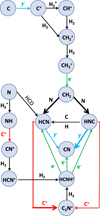 |
Fig. 14 Dominant chemical reactions in FUV-illuminated gas. |
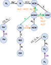 |
Fig. 15 Dominant chemical reactions in FUV-shielded gas. |
5.3 On HNC destruction reactions
Previous studies invoked that the isomerization reaction H + HNC → HCN + H determines a temperature dependence of the N(HCN)A/N(HNC) ratio in warm molecular gas (Schilke et al. 1992; Herbst et al. 2000; Graninger et al. 2014; Hacar et al. 2020). In our PDR models, the gas temperature is Γ ≃ 50 K at Av ≃ 1 mag, and T ≃ 15 K at AV 4 mag (upper panels of Fig. 13a and b). We run the same two models adopting Eb = 200 K for reaction (8) and found that reducing Eb has little effect on the predicted N(HCN)/N(HNC) ratio (blue continuous curves in the upper panels of Figs. 13a and b). Even at AV < 2 mag, where the abundance of H atoms and T are moderately high, the JV(HCN)/JV(HNC) ratio increases by less than 30% (i.e., the effects are very small). We note that in all these models, HCN and HNC photodissociation, as well as C + HNC → HCN + C reactions, are faster than the isomerization reaction H + HNC (see Figs. 13c and 13d).
We run a more extreme model adopting Eb = 0 K. That is to say, as if reaction (8) was barrierless. Only in this case, the isomerization reaction H + HNC → HCN + H would dominate HNC destruction (specially at large AV), increasing the N(HCN)/N(HNC) ratio. However, this choice of Eb results in very low HNC column densities, 2 × 1012 cm−2 and 3 × 1011cm−2 at Ay = 8 mag for nH = 5 × 103 cm−3 and 5 × 104 cm−3, respectively. These N(HNC) values are much lower than the N(HNC) column densities we infer from observations (Table E.l). In addition, models with Eb = 0 K would imply very high N(HCN)/N(HNC) = 30–75 ratios, something not seen in our observations (Table 8).
Some studies also suggest that in cold molecular gas, reaction HNC + O → CO + NH dominates HNC destruction, and thus it controls the HCN/HNC abundance ratio if the energy barrier of this particular reaction is low, Eb≃ 20–50 K (Schilke et al. 1992; Hacar et al. 2020). However, these values are much lower than the expected theoretical barrier (A. Zanchet, priv.comm. and Lin et al. 1992). Overall, our observational results are more consistent, at least for the extended cloud emission, with a greater dependence of the N(HCN)/N(HNC) ratio on the FUV radiation field (as suggested in planetary nebulae, Bublitz et al. 2019, 2022).
6 Discussion
In this section we discuss the nature of the extended HCN J= 1–0 emission observed in Orion B and its relation to other species. We conclude by comparing the observed line intensity vs. FIR dust continuum intensity scalings with the line luminosity vs. SFR scaling laws typically inferred in extragalactic studies.
6.1 The origin of the extended HCN J = 1–0 emission: weak collisional excitation vs. scattering
The existence of a widespread HCN J = 1–0 emission component in low density gas, weakly collisionally excited, but enhanced by electron collisions (see Sect. 4.3), may affect the interpretation of the extragalactic relationship HCN luminosity versus SFR. Alternatively, the extended HCN J = 1–0 emission we observe in Orion B might arise from photons emitted in dense star-forming cores that become resonantly scattered by halos of low density gas. This seems to be the case, albeit at much smaller spatial scales, in dense cores inside cold dark clouds shielded from stellar FUV radiation (e.g., Langer et al. 1978; Walmsley et al. 1982; Cernicharo et al. 1984b; Gonzalez-Alfonso & Cernicharo 1993).
The above two scenarios lead to different HCN J = 1–0 HFS line intensity ratios (see predictions by Goicoechea et al. 2022), which can be tested on the basis of HFS resolved observations of the extended gas emission in GMCs. In particular, if the observed HCN J = 1–0 HFS photons arise from dense gas and become resonantly scattered by interacting with a low density halo, then both the R02 and R12 HFS line intensity ratios should be very anomalous. That is, R02 < 0.2 and R12 < 0.6. On the other hand, if the HCN J = 1–0 emission intrinsically arises from low density gas, far from dense cores, models predict that weak collisional excitation drives the HFS intensity ratios to R02 ≳ 0.2 and R12 ≲ 0.6.
Figure 8a shows that the most common HCN J = 1–0 HFS line intensity ratios in Orion B are R02 ≳ 0.2 and R12 ≲0.6 (Fig. 7). Hence, the very anomalous ratios predicted by the scattering halo scenario are rarely encountered at large scales. Therefore, weconcludethattheextendedHCN J=1–0 emission in Orion B is weakly collisionally excited, and it mostly arises from low density gas. In particular, we determined n(H2) of several 103 cm−3 to 104 cm−3 (see Sect. 4.3). This result contrasts with the prevailing view of HCN J = 1–0 emission as a tracer of dense gas (e.g., Gao & Solomon 2004a,b; Rosolowsky et al. 2011; Jiménez-Donaire et al. 2017, 2019; Sánchez-García et al. 2022; Rybak et al. 2022).
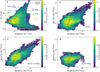 |
Fig. 16 2D histograms. (a) Visual extinction AV as a function of the HCN/CO J =1–0 integrated intensity ratio (from maps at 120″ resolution). Dashed red, yellow, green, and blue horizontal lines are the visual extinction values 1, 4, 8, and 15 mag, respectively. Above each line, we show the percentage of the total HCN J = 1–0 luminosity that comes from the different AV ranges. (b), (c), and (d) 2D histogram of the observed [C I] 492 GHz/CO J =1–0 line intensity ratio (in units of K km s−1) as function of the observed HCN/CO J =1–0 line ratio for all AV, for AV < 3 mag, and for AV > 3 mag. The dashed black curve shows the running median. Error bars show the standard deviation in the x-axis. |
6.2 Bimodal behavior of the HCN/CO J = 1–0 line intensity ratio as a function of AV
Extragalactic studies frequently interpret the HCN/CO J = 1–0 line luminosity ratio as a tracer of the dense gas fraction (e.g., Lada 1992; Gao & Solomon 2004b,a; Usero et al. 2015; Gallagher et al. 2018; Jiménez-Donaire et al. 2019; Neumann et al. 2023). This interpretation assumes that CO J =1–0 line emission is a tracer of the bulk molecular gas, whereas HCN J=1–0 traces dense gas in star-forming cores (at high AV). Normal galaxies have low luminosity ratios LHCN/LCO = 0.02–0.06 while luminous and ultraluminous galaxies have LHCN/LC0 > 0.06. By contrast, Helfer & Blitz (1997) argue that the HCN/CO intensity ratio could measure the total hydrostatic gas pressure.
Figure 16a shows a 2D histogram of the HCN/CO J=1–0 line intensity ratios in Orion B as a function of AV. The 2D histogram shows a bimodal behavior. There is a first branch at AV > 3 mag where W(HCN)/W(CO) J=1–0 increases with extinction (the assumed behavior in extragalactic studies). The running median W(HCN)/W(CO) J=1–0 ratio increases from ≳ 0.02 (at AV ≃ 8 mag) to ~0.1 (dense cores at larger AV). In addition, there is a second branch at AV < 3 mag where W(HCN)/W(CO) J=1–0 increases with decreasing extinction. This is somehow unexpected, because the running median intensity ratio reaches high values, ≳ 0.1, in diffuse gas at AV ≃ 1 mag.
Figure 6a shows the spatial distribution of the HCN/CO J =1–0 intensity ratios in Orion B. The ratio is indeed high toward the dense gas in filaments and cores. In addition, W(HCN)/W(CO) J = 1–0 also increases toward the east rim of the cloud that borders the ionization front IC 434. Owing to the roughly edge-on geometry with respect to the illuminating stars, we can easily spatially resolve these FUV-illuminated cloud edges (high χe) from the more shielded cloud interior. This picture agrees with HCN J =1−0 emission arising from extended and relatively low density gas, n(H2) ≤ 104 cm−3, in GMCs illuminated by FUV radiation, and being boosted by electron excitation. This extended cloud component must be common in GMCs that host young massive stars, or have massive stars in their vicinity.
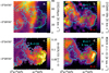 |
Fig. 17 30″-resolution view of the Horse-head. (a) [C II] 158 µm (Pabst et al. 2017) and (b) [C I] 492 GHz (Philipp et al. 2006) integrated line intensity maps (from 7 to 18 km s−1). (c) R = HCN/CO intensity ratio and (d) HCN J = 1−0 line intensity maps. Contours on [C II] 158 µm map: HCN/CO ratio (R = 0.06 and 0.12). Contours on [C I] 492 GHz map: HCN J =1−0 surface brightness (W = 2.7, 4.5, and 6 K km s−1). |
6.2.1 Cloud porosity to FUV radiation: HCN 1−0 emission from high electron abundance gas traced by [C II] 158 µm and extended [C I] 492 GHz emission
The ionization fraction in cloud edges and in gas translucent to FUV-radiation is high. It starts at χe ≃ a few 10−4, where the electron abundance is controlled by the photoionization of carbon atoms, thus leading to χe ≃;χ(C+) at AV ≲ 2 mag. These cloud layers emit bright FIR [C II] 158 µm fine-structure line emission. Slightly deeper inside the molecular cloud, at AV ≲ 3 mag, the flux of FUV photons decreases to the point where the gas becomes fully molecular, and neutral atomic carbon (C0) becomes more abundant than C+ (see PDR models in Figs. 13a and b). Our models predict χe ≳ 10−5 at the C0 abundance peak, where the [C I] 492 GHz line emission reaches its intensity peak.
Figure 17a shows a [CII] 158 µm line emission map of the Horsehead nebula and the ionization front IC 434 observed with SOFIA (Pabst et al. 2017) and convolved to the 30″ resolution of the ORION-B maps. The C+ map shows faint [C II] 158 µm emission from the (nearly edge-on) molecular PDR at the rim of the Horsehead. It also shows bright [C II] 158 µm emission from the neutral atomic PDR, χ(H) ≫χ(H2) at AV < 1 mag, that delineates the edge of IC 434 and shows very little CO emission (e.g., Bally et al. 2018). Figure 17c shows a closer look to the HCN/CO J = 1−0 line intensity ratio. The ratio is particularly high, ≥ 0.12 (green contours), toward the FUV-illuminated cloud edge. This area matches the [C II] 158 µm emission from the rim of the Horsehead. As n(H2) is a few 104 cm−3 (e.g., Pabst et al. 2017) and  (HCN J = 1−0) <χe ≃;χ(C+) ≃ 10−4, electron excitation boosts the HCN emission (see Fig. 10), and thus the HCN/CO J = 1−0 line intensity ratio.
Figure 17b shows a map of the [C I] 492 GHz line emission around the Horsehead nebula observed with Caltech Submillimeter Observatory (Philipp et al. 2006) and smoothed to 30″ resolution. The HCN J =1−0 emission nicely follows that of [C I] 492 GHz. This agrees with the widespread nature of neutral atomic carbon, and with the similar spatial distribution of [C I] 492 GHz and HCN J = 1−0 emission seen at much larger scales (cf., the complete Orion B maps in Fig. 2h). This observational result indicates that C0 coexists with HCN in large areas of the cloud, which implies moderate ionization fractions, χe ≳ 10−6 to several 10−5, in gas where [C I] 492 GHz and HCN J =1−0 emissions coexist.
Since the spatial and velocity distribution of the large-scale [C I] 492 GHz and13CO J = 1−0 emission are very similar (Ikeda et al. 2002), the presence of C0 cannot be restricted to cloud edges (AV < 3 mag). Otherwise Fig. 2h would only show bright [C I] 492 GHz emission parallel to the IC 434 front associated with the rims of all nearly edge-on PDRs such as the Horse-head (zoomed in Fig. 17). Instead, the [C I] 492 GHz emission is widespread and extended through the cloud. We find that [C I] 492 GHz also linearly correlates with the HCO+, HCN, and 13CO J = 1–0 emission (Pearson coefficients of 0.80, 0.79, and 0.73 respectively). These correlations include many positions at AV > 3 mag (60% of [C I] 492 GHz detections, and 70% of total [C I] 492 GHz luminosity, see Fig. 4). Therefore, C0 must be abundant also toward the cloud interior. The most plausible scenario suggested by these maps is that GMCs are porous to FUV radiation. This is consistent with the detection of very extended 70 µm dust emission from FUV-illuminated grains (see Fig. 1). This implies that GMCs are inhomogeneous, and we are detecting [C I] 492 GHz emission from the cloud edges as well as from FUV-illuminated surfaces of structures located at moderate cloud depths (typically modeled as clumps, filamentary, or fractal structures, e.g., Boisse 1990; Falgarone et al. 1991; Spaans 1996; Stutzki et al. 1998; Barnes et al. 2013). Unfortunately, while ALMA, Keck, and JWST observations show surprisingly rich small-scale substructures in the prototypical PDR the Orion Bar (Goicoechea et al. 2016; Habart et al. 2023a,b), similar sub-arcsecond resolution observations of the [C I] 492 GHz are still missing. Such observations will help to constrain the small-scale origin of C0.
6.2.2 High HCN/CO J = 1−0 and [C I] 492 GHz/CO J = 1−0 line intensity ratios from gas at AV < 3 mag
We close our discussion of the bimodal behavior of the W(HCN)/W(CO) J =1−0 intensity ratio by providing more evidence that FUV radiation (leading to abundant C0 and moderate χe) is ultimately responsible of the increased ratios observed at AV < 3 mag (Fig. 16a). These regions correspond to translucent gas and FUV-illuminated cloud edges. They coincide with enhanced [C I] 492 GHz/CO J =1−0 line intensity ratios (Fig. 6), which traces low-density PDRs (Hollenbach et al. 1991; Kaufman et al. 1999). Hence, we expect that both ratios are related.
Figure 16 shows the distribution of [C I] 492 GHz/CO J = 1−0 and HCN/CO J =1−0 intensity ratios in Orion B. The upper-right panel shows all detections (at all AV) in the map. The running median clearly shows that, above a threshold of W(HCN)/W(CO) J = 1−0 ≳ 0.02, the ratio quickly increases with the [C I] 492 GHz/CO J =1−0 intensity ratio. The lower panels in Fig. 16 separate the HCN/CO and [C I]/CO detections in the lines of sight with AV < 3 mag (Fig. 16c) and AV > 3 mag (Fig. 16d). These plots show that the HCN/CO J = 1−0 line intensity ratio linearly correlates with [C I] 492 GHz/CO J = 1−0 at AV < 3 mag. Hence, the ratios follow the increasing electron abundance in PDR gas. On the other hand, the ratios are not correlated at higher AV > 3 mag. As a corollary, our observations imply that the detection of high HCN/CO J = 1−0 line intensity ratios do not always imply the presence of dense gas. The existence of a low-AV branch, from extended FUV-illuminated low-density gas, leads to increasing ratios with decreasing AV. This cloud component cannot be overlooked, specially in the context of the very large scale emission from GMCs, otherwise the mass of the dense molecular gas can easily be overestimated. In the next section we specifically quantify the amount of dense molecular gas traced by the HCN J = 1−0 emission.
6.3 The dense gas mass conversion factor α (HCN J = 1−0)
Using the dust SEDs across the observed field10, we derive the mass of the dense gas in the mapped area (represented by gas at AV > 8 mag, e.g., Lada et al. 2010). The likely density of this cloud component is n(H2) > 104 cm−3 (e.g., Bisbas et al. 2019). We obtain Mdg = 3.1 × 10³ M⊙, which accounts for about 20% of the total mass ( M⊙) in the mapped area. These numbers imply a dense gas surface density (Σdg = Mdg/A) and a total gas surface density (
 ) of Σdg = 13 M⊙ pc−2 and
  , respectively, where in both cases we divide by the total mapped area, A ≃ 250 pc2.
High spatial resolution observations of the dust SED are rarely available in extragalactic studies. Hence, it is appropriate to calibrate the mass of the dense molecular gas with the emitted luminosity of a convenient molecular line tracer, with HCN J = 1−0 being the traditional choice. Hence, it is common to define:
 (12)
(12)
where L′(HCN) is the total HCN J =1−0 line luminosity in the mapped area (in K km s−1 pc2) as defined in Eq. (4). Gao & Solomon (2004a) originally estimated α(HCN) = 10 M⊙ / K km s−1 pc2. Recent dust continuum and line emission surveys determine α(HCN) in a few local GMCs (e.g., Shimajiri et al. 2017; Kauffmann et al. 2017; Barnes et al. 2020). These studies find quite a diversity of α(HCN) values, from 10 to 500 M⊙/K km s−1 pc2. However, these surveys typically map star-forming clumps and their immediate environment (areas <1 deg2) but do not account for, or do not spatially resolve, the extended HCN J=1−0 emission from low density and more translucent gas. This emission is weakly excited (TCMB ≲ Tex ≪ Tk), but because it covers large spatial scales, its total line luminosity typically exceeds the line luminosity from dense gas in star-forming cores at AV > 8 mag (~30% in Orion B).
Here we determine α for HCN, HCO+, and HNC J = 1−0 lines in OrionB. We obtain L′(HCN)=110 K km s−1 pc2 for HCN J = 1−0, which implies a dense mass conversion factor α(HCN) = 29 M⊙/K km s−1 pc2. Table 4 summarizes the luminosities and α values derived for other molecules. A recent survey of the Perseus low-mass star-forming region (at 11 arcmin resolution and covering 8.1 deg2 or ~215pc2) finds α(HCN) = 92M⊙/K km s−1 pc2, L′(HCN) = 55.3 K km s−1, and Mdg = 5.1 × 10³ M⊙ (Dame & Lada 2023). As FUV radiation favors the formation of HCN and the excitation of the J = 1−0 line at large spatial scales (enhanced by electron collisions; Sect. 6.1), our study suggests that the lower α(HCN) value in Orion B is linked to the presence of FUV radiation from massive stars. Indeed, Shimajiri et al. (2017) mapped small areas of Orion B, Aquila, and Ophiuchus star-forming cores (<10pc2). They find that α(HCN) anticorrelates with G0. We do find this tendency at the much larger spatial scales of our maps, but not a strong anticorrelation. This can be explained by the nonlinear dependence of the HCN abundance, HCN J = 1−0 line emission, and electron abundance with G0.
All in all, we conclude that there is no universal α(HCN J = 1−0) value, as environmental conditions and contribution of the low density extended cloud component at different angular scales likely vary from cloud to cloud. In Orion B, the cloud mass at AV > 8 mag is similar to that at AV < 3 mag. This results in a similar value of the mass to total L′(HCN) ratio in both cloud components. Thus, it will not be straightforward to distinguish, based on the observation of a single line, which component dominates the emission from spatially unresolved GMCs.
6.4 Schmidt-like laws: Spatially resolved relations between molecular and atomic lines with FIR intensities
On more global spatial scales (hundreds of parsec to kilopar-sec scales) than those discussed in our study, observations of nearby normal galaxies find a tight, close to linear, correlation between the HCN J = 1−0 line luminosity and the FIR luminosity (a proxy of the SFR when averaged on such global scales; Solomon et al. 1992; Gao & Solomon 2004a; Kennicutt & Evans 2012). However, when considering starburst galaxies and (U)LIRGs, the relation often deviates from linearity (e.g., Gao et al. 2007; García-Burillo et al. 2012; Usero et al. 2015; Sánchez-García et al. 2022). These luminous galaxies lie above the FIR-HCN correlation observed in nearby normal galaxies. They also display high HCN/CO J = 1−0 line luminosity ratios (~ 0.2) interpreted as galaxies having high fractions of dense molecular gas. Our survey of Orion B provides access to the local properties that contribute to the large averages seen in galaxies. In this section we discuss the spatially resolved relationships between IFIR and CO, HCN, HCO+, HNC J = 1–0, and [C I] 492 GHz line intensities (W) mapped in Orion B.
Figure 18 shows 2D histograms of the observed W(CO), W(HCN), W(HCO+), W(HNC), and W([C I] 492 GHz) line intensities (in K km s−1) as a function of IFIR (in erg s−1 cm−2 sr−1). We find that the observed line intensities W scale with IFIR as a power law. As we fit these points using an orthogonal regression method11 in log(y)-log(x) space and we use the appropriate error bars (the standard deviation) in both axes, we can present the scalings as IFIR ∝ WN (as in Fig. 18) or as  (as in Fig. B.3). Perhaps provocatively, and in order to promote the comparison with the extragalactic scalings SFR–Lmol (e.g., Gao & Solomon 2004a; Shirley et al. 2008; Shetty et al. 2013, 2014a,b), here we start discussing the power-law indexes N.
As discussed in Sect. 2.5, IFIR is a surrogate of the local FUV radiation field,  (upper panel x-axis of Fig. 18). FUV photons are related to the presence of massive O and B stars that have short lifetimes. Thus, the FIR emission from FUV-heated grains is ultimately related to the SFR. However, the statistical connection between SFR and FIR luminosities in galaxies holds when averaging over large cloud samples (e.g., Kennicutt & Evans 2012). Therefore, the extrapolation of the local scalings in Orion B to galaxies (global averages) has to be taken with caution, bearing in mind that IFIR traces the strength of the FUV radiation field, but LFIR over a small region does not trace the true SFR12.
By fitting all points in Fig. 18, we find that W(CO), W(HCO+) and W(HCN J = 1–0) scale with IFIR as a power law with N ~ 0.9–1.3. However, W(HNC J = 1–0) and W([C I] 492 GHz) show a different behavior, with a power-law index N ~ 1.8–2.2. A closer inspection of the IFIR–W(CO J = 1–0) running median shows two clear tendencies. The median toward the brightest FIR positions (IFIR > 0.4 erg s−1 cm−2 sr−1 or  , mostly arising from NGC 2024 star-forming clump) shows a power-law index of N~ 4.8. On the other hand, the faintest IFIR and W(CO J = 1–0) positions show N ~ 0.4 (sublinear relationship). This faint CO emission is associated with widespread and very extended diffuse gas (low AV and G′0<20).
The IFIR–W(HCN J = 1–0) and IFIR–W(HCO+ J = 1–0) histograms are quite similar. They also reveal two different tendencies. Fitting the brightest IFIR positions alone, most of them associated with dense gas in NGC 2024 (as demonstrated by the detection of bright HCN J = 4−3 line emission, Fig. 3), provides N~1.6 for HCN and N~2.4 for HCO+ (superlinear relationships). In contrast, the most common low surface brightness HCN J = 1–0, HCO+ J = 1–0, and IFIR positions (those with  ) show N~0.6 (i.e., not far from the extended and diffuse CO emission index). Interestingly, the IFIR–W(HNC J = 1–0) and IFIR–W([C I]492 GHz) histograms show a single superlinear tendency across the map, with N~1.8 and 2.2, respectively. Hence, HNC and [C I] 492 GHz have a very different behavior compared to the other species. The derived N index for HNC resembles the index we find for HCN at the highest values of IFIR (
 and dense gas), whereas the single index for [C I] 492 GHz resembles that of HCO+ at high G′0. This similitude must reflect their related chemistry and excitation conditions.
From the point of view of the local gas properties, Figs. 18 and B.3 show that W(CO J = 1–0), W(HCO+ J = 1–0), and W(HCN J = 1–0) intensities increase with increasing IFIR up to G′0 ≃ 20. Most of these positions refer to the extended cloud component, which hosts low densities and thus, the HCN J = 1–0 line is weakly collisionally excited (see Sect. 4.3), with n(H2) < ncr, eff(HCN 1–0) and thus, Tex < Tk. Under these conditions (effectively thin emission), W(HCN J = 1–0) scales with N(HCN) even for large line opacities (see also Liszt & Pety 2016). Furthermore, our chemical analysis shows that models with a higher G0/nH ratio produce more HCN (Sect. 5 and Fig. 13). In addition, electron excitation contributes to enhance W(HCN J = 1–0) at low densities. These conditions favor the emission of CO, HCO+, and HCN as G′0 increases.
On the other hand, Figs. 18 and B.3 show that W(CO J = 1–0), W(HCO+ J = 1–0), and W(HCN J = 1–0) respond weakly to IFIR once the FUV field becomes too intense ( ). These other regions at large AV host denser gas, so that n(H2) > ncr, eff(HCN 1–0), and J = 1–0 lines turn into very optically thick, thus becoming less sensitive to column densities. Interestingly, W(HNC J = 1–0) and W([C I] 492 GHz) weakly respond to IFIR at all G′0. We already showed that HNC traces slightly denser gas than HCN (Fig. 5c) and that HNC responds less to electron excitation (Table 1). In addition, the observed W(HCN 1–0)/W(HNC 1–0) intensity ratio increases with the FUV field for G′0 < 200 (Fig. 12). Indeed, our chemical models show that the HNC abundance is lower in the FUV-illuminated gas (Sect. 5). This gas is usually at lower density than the FUV-shielded cold gas. Thus, we expect that most of the HNC J = 1–0 emission arises from gas in which n(H2) > ncr, eff (HNC 1–0). These facts explain the weaker response of W(HNC J = 1–0) to FUV radiation. Finally, PDR models predict that the C0 column density is a weak function of gas density and especially of G0 (e.g., Hollenbach et al. 1991). This is consistent with the weak scaling we find in Orion B.
As a corollary, we conclude that our large-scale and spatially resolved lines maps of a local GMC show a variety of power-law indexes, IFIR ∝ WN (or  ). These N indexes resemble the kind of Kennicutt-Schmidt power-law indexes,
  , found in galaxy surveys that average multiple GMCs (e.g., Wu et al. 2005, 2010; Kennicutt & Evans 2012; García-Burillo et al. 2012; Sánchez-García et al. 2022). We attribute the different scalings in Orion B to the different gas densities, excitation regimes, and chemistry of the star-forming (dense and compact) versus non-star-forming (low density, extended, and FUV-illuminated) environments. However, while it is tempting to extrapolate our results to the extragalactic scalings (as in Krumholz & Thompson 2007; Narayanan et al. 2008), we still need to better understand the spatial scales at which LFIR becomes a reliable tracer of the global SFR, as well as the connection between the extragalactic averages versus our spatially resolved scalings.
 |
Fig. 18 2D histograms of the 12CO, HCN, HCO+, HNC, J = 1–0, and [C I]3P1 – 3P0 line intensities as a function of FIR intensity in Orion B (from maps at 120″ resolution). The dashed red lines show the running median (median values of the integrated intensity within equally spaced log IFIR bins). The error bars show their dispersion. Black lines (and associated text) show a linear fit (orthogonal regression in log(y)-log(x)) to all observed positions in each map. Magenta lines and blue lines show a linear fit to a range of IFIR <6 × 10⁻³ erg s−1 cm−2 sr−1 and (0.4–7.7) erg s−1 cm−2 sr−1, respectively. We note that in each plot the number of line detections is different. |
7 Summary and conclusions
In the context of the IRAM 30m ORION-B large program, we presented a detailed analysis of 5 deg2 (~250 pc2) HCN, HNC, HCO+, CO J = 1–0, and [C I]492 GHz line emission maps of the Orion B GMC. We complemented this dataset with new pointed observations of rotationally excited HCN, HNC, H13CN, and HN13C lines. We constructed integrated line intensity (W), visual extinction, and IFIR (a proxy of G0) maps from existing dust SED observations. We summarize our results as follows:
About 70% of the total HCN J = 1–0 luminosity, L′(HCN J = 1–0) = 110 K km s−1 pc−2, arises from gas at AV < 8 mag (Sect. 3.1), that is, from gas below the common extinction threshold of star-forming cores. About 80% of the total cloud mass and 50% of the total FIR luminosity (mostly arising from FUV-heated dust grains) also stems from AV < 8 mag.
We detect anomalous HCN J = 1–0 HFS line intensity ratios (also in the HCN J = 2−1 and 3−2 transitions) almost everywhere in the cloud (Sect. 4.4). That is, HCN J = 1–0 R02 = W(F = 0–1)/W(F = 2−1) and R12 = W(F = 1–1)/W(F = 2−1) hyperfine line intensity ratios outside the LTE range R02 = [0.2, 1] and R12 = [0.6, 1]. We also detect anomalous HFS line width ratios. That is, Δυ(F = 0–1) ≠ Δυ(F = 2−1) ≠ Δυ(F = 1–1) (Sect. 4.2). Radiative effects induced by moderate line opacities and HFS line overlaps produce these anomalous ratios, which are inconsistent with the common assumption of the same Tex and line width for all HFS lines of a given rotational transition.
Most of the widespread and extended HCN J = 1–0 emission arises from weakly collisionally excited gas with n(H2) ≲ 104 cm−3. That is, it is not line radiation emitted by dense cores that is resonantly scattered by low density halos (Sect. 6.1). This is demonstrated by the typical HCN J = 1–0 HFS intensity ratios R02 ≳ 0.2 and R12 < 0.6 observed at large scales. Even lower densities are possible in FUV-illuminated gas if χe ≥ 10−5 and electron collisional excitation dominates (Sect. 4.3).
The HCN/HNC J = 1–0 line intensity ratio is sensitive to the strength of the FUV radiation field. Our chemical models and observations suggest that the HCN/HNC abundance ratio is more sensitive to G0 than to Tk (Sect. 5). In particular, HNC is a slightly better tracer of dense gas, defined as n(H2) > 104 cm−3, than HCN, because its abundance is lower in the FUV-illuminated gas (translucent gas and cloud edges). This gas is usually at lower density than the FUV-shielded cold gas. In addition, HNC is less sensitive to electron excitation than HCN (Table 1).
The HCN/CO J = 1–0 line intensity ratio (Sect. 3.2), widely used as a tracer of the dense gas fraction, shows a bimodal behavior with respect to AV, with an inflection point at AV ≲ 3 mag (Sect. 6.2) typical of translucent gas and FUV-illuminated cloud edges. The extended cloud HCN J = 1–0 emission (Sect. 4.3) explains the low AV branch of the observed distribution of the HCN/CO J = 1–0 line intensity ratio. The highest HCN/CO J = 1–0 line intensity ratios (~ 0.1) at AV < 3 mag correspond to regions displaying high [C I] 492 GHz/CO J = 1–0 intensity ratios too (> 1). These values are characteristic of low-density PDRs and χe ≳ 10−5. Therefore, we conclude that the detection of high HCN/CO J = 1–0 intensity ratios does not always imply the presence of dense gas.
Given the widespread and extended nature of the [C I]492GHz emission (a typical tracer of PDR gas), and its spatial correlation with W(HCO+ J = 1–0), W(HCN J = 1–0), and W(13CO J = 1–0) (see Sect. 6.2.1), the extended component of Orion B (and likely in most GMCs), must be porous to FUV radiation from nearby massive stars. Indeed, 70% of the total [C I] 492 GHz luminosity arises from lines of sight with AV > 3 mag (i.e., not exactly from the cloud surface). In addition, the 70 µm continuum emission from FUV-illuminated dust grains is very extended. The enhanced FUV field favors the formation of HCN and the excitation of the J = 1–0 line at large scales, not only in dense star-forming cores. This is exemplified by the relatively low value of the dense gas mass to the HCN J = 1–0 line luminosity ratio, α (HCN) = 29 M⊙/K km s−1 pc2, in Orion B (Sect. 6.3). The existence of a widespread HCN J = 1–0 emission component associated with low density gas affects the interpretation of the extragalactic relationship LHCN versus SFR.
The low-surface brightness and extended HCN J = 1–0 and HCO+ J = 1–0 emissions (≲ 1 K km s−1) scale with IFIR with a similar power-law index (Sect. 6.4). Together with CO J = 1–0, these lines respond to the increasing IFIR up to G′0 ≃ 20. On the other hand, the bright HCN emission (> 6 K km s−1) from dense gas in star-forming clumps weakly responds to IFIR once the FUV radiation field becomes too intense (G′0 > 1500). HNC J = 1–0 and [C I] 492 GHz lines weakly respond to IFIR at all G′0.
Our large-scale and spatially resolved lines maps of a local GMC show a variety of power-law indexes, IFIR ∝ WN (from sublinear to superlinear), that resemble the kind of Kennicutt-Schmidt power-law indexes,
 , found in surveys of different galaxy types that spatially average multiple GMCs (e.g., Kennicutt & Evans 2012). We attribute the different scalings in Orion B to the different gas densities, excitation regimes, and chemistry of the star-forming (compact) versus non-star-forming (extended) environments (Sect. 6.4).
Our study stresses the major contribution of the extended and low density component of GMCs to the total CO, HCO+, and HCN J = 1–0 line luminosity. It also enables us to remark that there is a need to carry out sensitive wide field surveys of galactic GMCs in multiple molecular lines. This will allow us to determine the properties of the star formation environment and to better understand the origin of the extragalactic Kennicutt-Schmidt scalings on global galaxy averages. In Orion B, the HCN J = 1–0 line intensity at any position of the extended cloud component is obviously much fainter than that arising from dense star-forming clumps such as NGC 2024. However, the much larger area of the extended cloud component at low AV implies that the emission arising from dense cores does not dominate the HCN J = 1–0 line luminosity from GMCs (see also Santa-Maria et al. 2021). Finally, better knowledge of the rate coefficient of some critical gas-phase reactions, namely reaction NCO + N → HCN + O and reactions of HNC with H, C, and O atoms, will help us to refine our abundance estimations from chemical models.
Acknowledgements
We are very grateful to our referee for a very detailed and constructive report that allowed us to improve the presentation of our results. M.G.S.M. and J.R.G. thank the Spanish MICINN for funding support under grant PID2019-106110GB-I00. This work was supported by the French Agence Nationale de la Recherche through the DAOISM grant ANR-21-CE31–0010, and by the Programme National “Physique et Chimie du Milieu Interstellaire” (PCMI) of CNRS/INSU with INC/INP, co-funded by CEA and CNES. Part of this research was carried out at the Jet Propulsion Laboratory, California Institute of Technology, under a contract with the National Aeronautics and Space Administration (80NM0018D0004). We thank A. Zanchet for useful discussions on the energy barrier of the HNC + H and HNC + O reactions and A. Faure for providing the HFS-resolved rate coefficients for HCN-e− inelastic collisions. This work is based on observations carried out under project number 019-13, 022-14, 145-14, 122-15, 018-16, the large program number 124-16, 130-21, and 127-22 with the IRAM 30m telescope. IRAM is supported by INSU/CNRS (France), MPG (Germany), and Spain (ING). This research made use of data from the Herschel Gould Belt survey (HGBS) project (http://gouldbelt-herschel.cea.fr). The HGBS is a Herschel Key Programme jointly carried out by SPIRE Specialist Astronomy Group 3 (SAG 3), scientists of several institutes in the PACS Consortium (CEA Saclay, INAF-IFSI Rome and INAF-Arcetri, KU Leuven, MPIA Heidelberg), and scientists of the Herschel Science Center (HSC).
Appendix A Main regions in Orion B
In this Appendix we provide more details about the properties of the main regions in Orion B discussed in this work (see Fig. 2).
NGC 2024: also known as the Flame nebula, is located east of the belt star Alnitak (ζ Ori). This is an active massive star-forming region, with the highest H2 column density (~5×1023 cm−2) and star formation efficiency (SFE~30%, Lada et al. 1997) in Orion B. It is composed of an embedded stellar cluster and associated H II region (Barnes et al. 1989). Inside the molecular ridge behind the H II region, FIR and radio observations reveal the presence of embedded dense cores, protostars, and YSOs (Mezger et al. 1988; Gaume et al. 1992; Chandler & Carlstrom 1996; Choi et al. 2015; Ren & Li 2016; Könyves et al. 2020). The bulk of the FIR line emission arises from an extended PDR, with Tk ≃ 75-100 K and n(H2)≃106 cm−3. This region is illuminated by ionizing and dissociating UV photons from a massive star (e.g., Giannini et al. 2000; Emprechtinger et al. 2009). The dominant ionizing source is likely the late-O or early-B star IRS2b (Bik et al. 2003; Meyer et al. 2008).
NGC 2023: is a reflection nebula located 20′ south of NGC 2024 (Meyer et al. 2008). It is illuminated by a B1.5V star (Abt & Levato 1977). This is a filamentary massive star-forming region (Könyves et al. 2020; Gaudel et al. 2023), with a FUV radiation flux equivalent to a few 104 times the mean interstellar radiation field (G0) toward the [C II] 158 µm emission peak (e.g., Sandell et al. 2015).
The Horsehead nebula13: also known as Barnard 33, is a dense pillar seen projected against the bright H II region and ionization front IC 434. The multiple stellar system, σ Orionis, formed by an O9.5V and a B0.5V binary, photoionizes the region (Walter et al. 2008). The Horsehead and all the western rim of the Orion B cloud is a large scale PDR eroded by UV radiation from σ Ori. The molecular cloud is located at a projected distance of ~4 pc from the ionizing stars, resulting in a moderate incident FUV flux, G0 ≃ 100 (Abergel et al. 2003). The expansion of the H II region likely triggers gas compression along the cloud rim and perhaps star-formation (Bally et al. 2018). The Horse-head pillar points radially to the ionizing source, and its western edge is a PDR observed nearly edge-on. This region hosts a few dense cores, protostars and YSOs (Bowler et al. 2009; Könyves et al. 2020). The gas temperature ranges from ~100 K (at the FUV-illuminated edge) to 10-20 K deeper inside the cloud (e.g., Habart et al. 2005; Pety et al. 2007; Goicoechea et al. 2009).
Orion B9: is an active low-mass star-forming region composed of supercritical filaments hosting pre- and proto-stellar cores (Miettinen et al. 2009, 2010). Line observations resolve two different velocity components at about υLSR=0-4 km s−1 and 8-10 km s−1, respectively (e.g., Gaudel et al. 2023).
The Flame filament: is physically connected with NGC 2024, at the southeast of NGC 2024. This is a very structured filament (Orkisz et al. 2019; Gaudel et al. 2023).
The Hummingbird filament: is one of the longest isolated filaments in the observed field. Only a few embedded YSOs exist in this region (Orkisz et al. 2019).
The Cloak: is a filamentary structure that crosses Orion B from east to west (Gaudel et al. 2023). Embedded starless and prestellar cores exist in the region (Könyves et al. 2020).
Appendix B Line intensities, line intensity ratios, and their relation to AV and IFIR
In this Appendix we show 2D histograms that display the relationship between line intensity ratios, AV, and IFIR. In Sect. 6.2 we discussed the behavior of the HCN/CO J = 1–0 line intensity ratio with AV and its relation to the [C I]/CO J = 1–0 line intensity ratio. In Sect. 5.3 we discussed the HCN/HNC abundance ratio and its possible relation with G0. In addition, Fig. B.3 shows 2D histograms of the relation between line intensities and IFIR, showing the exponents  (see Sect. 6.4).
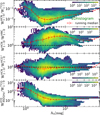 |
Fig. B.1 2D histograms showing the line intensity ratios HCN/CO, HCN/HNC, HCN/HCO+ J = 1–0, and [C I] 492 GHz/CO J = 1–0 with respect to the visual extinction AV. The dashed red line marks the running median. The error bars mark the standard deviation. The dashed black line marks the intensity ratio equal to one. |

Appendix C SED-derived parameters
C.1 Dust temperature and column density maps
In previous papers (e.g., Pety et al. 2017), we have used dust temperature and column density maps derived from the maps published by Lombardi et al. (2014), based on Herschel and Planck data. More recently, similar maps have been published by Könyves et al. (2020) as part of the HGBS (André et al. 2010; Schneider etal. 2013)14.
The Könyves et al. (2020) maps benefit from additional Her-schel observations, which were used to correct a small patch of pixels where the SPIRE detectors are saturated in the NGC 2024 region in the original data (Fig. C.1). This saturation creates an artifact in the maps derived by Lombardi et al. (2014). However, the two datasets, which in principle use essentially the same observational data and the same derivation method (modified black-body SED fitting) display some discrepancies (typically a factor of 1.2 – 1.5 in temperature and a factor 1.2 – 2 in column density), which can partly be attributed to the fact that Könyves et al. (2020) use a fixed value of zero-point calibrations for the Herschel bands and a fixed β index for the modified black body, whereas Lombardi et al. (2014) use spatially varying values for these parameters based on previous SED fitting of Planck and IRAS data.
For the sake of consistency with our previous work and due to the level of detail of its SED fitting, we chose to keep the Lombardi et al. (2014) data as our reference, but we incorporated the newly available reobserved patch in NGC 2024 by rescaling the Könyves et al. (2020) maps and compositing them into the Lombardi et al. (2014) maps (hereafter K20 and L14 maps respectively), as illustrated in Fig. C.1.
The compositing procedure for both column density and temperature was the following:
The saturated patch in NGC 2024 is masked out as tightly as possible, with a 81″ × 216″ (9 × 24 pixels) mask.
A 36″ wide (4 pixels, about one beam) border is selected around the masked patch, yielding a 153″ × 288″ selection region.
-
From this we obtain a correction constant AX corresponding to the local ratio between the datasets:
 (C.1)
(C.1)where X corresponds to N or T.
The 153″ × 288″ binary mask is then smoothed with a Hann window of radius 45″ (4/3 beam) to avoid compositing artifacts. This yields a gray-scale mask M, with value 1 in most of the map, 0.5 at the edge of the compositing region, and 0 at the center of the NGC 2024 region.
-
The two datasets are finally merged into a final column density map N or a final temperature map T:
 (C.2)
(C.2)where again X corresponds to N or T.
No significant discontinuity is visible in the combined datasets. Figure C.2 shows the spatial distribution of the dust temperature, the visual extinction, and integrated FIR intensity which are derived from these maps.
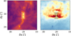 |
Fig. C.1 Compositing geometry in the NGC 2024 region between data from Lombardi et al. (2014) and Könyves et al. (2020), for column density (left) and dust temperature (right). The outer contour is the one in which the compositing is executed. The “selection area” over which the K20 datasets are rescaled to match the L14 ones corresponds to the outer contour minus the inner, hashed area (affected by the artifact in L14 and masked out). The full maps corresponding to these zoom-ins can be found in Fig. C.2 |
C.2 Determination of gas masses
We determined the mass of molecular gas as:
 (C.3)
(C.3)
where N(H2)=1.9×10²¹ AV, µ=2.8 is the molecular weight per H2, mH is the hydrogen atom mass, and Apixel is the area of each pixel in cm2. In Orion B, the total H2 mass is  . The dense gas mass, Mdg, was computed for visual extinctions AV >8 mag (e.g., Lada et al. 2010; Shimajiri et al. 2017).
Appendix D HCN hyperfine structure analysis
D.1 HCN J = 1–0 LTE-HFS fitting method
In Sect. 4.1 we determined Tex(J=1–0) and the opacity corrected column density Nτ,corr(HCN) by applying the LTE-HFS fitting method implemented in CLASS foot note 2. This method uses as input the line separation and the intrinsic line strengths of the J=1–0 HFS components, 1:5:3 (so that S = 9). The method assumes that the three HFS lines have the same Tex and linewidth Δυ. The output parameters are the linewidth Δυ = p3, the velocity of the reference component υLSR = p2, the sum of all the line center opacities such as p4 S = ∑ τHFS,I, and the product of the antenna temperature and the line opacity  . This procedure allows one to derive the (LTE) excitation temperature as:
 (D.1)
(D.1)
where Tbg is the background temperature (~2.73 K), and Feff/Beff is the ratio of the telescope forward and beam efficiencies (see CLASSfootnote 2 documentation). From the opacities and Tex, we derive the opacity corrected column density, assuming Boltzmann populations at a single Tex value:
![${N^{\tau ,{\rm{corr}}}} = {{8\pi {v^3}} \over {{A_{{\rm{ul}}}}\,{c^3}}}{{Q\left( {{T_{{\rm{ex}}}}} \right)} \over {{g_{\rm{u}}}}}{{{e^{{{{E_{\rm{u}}}} \mathord{\left/ {\vphantom {{{E_{\rm{u}}}} {k{T_{{\rm{ex}}}}}}} \right. \kern-\nulldelimiterspace} {k{T_{{\rm{ex}}}}}}}}} \over {{e^{{{hv} \mathord{\left/ {\vphantom {{hv} {k{T_{{\rm{ex}}}}}}} \right. \kern-\nulldelimiterspace} {k{T_{{\rm{ex}}}}}}}} - 1}}{{{W_{F = 2 - 1}}} \over {\left[ {{J_v}\left( {{T_{{\rm{ex}}}}} \right) - {J_v}\left( {{T_{{\rm{bg}}}}} \right)} \right]}}{{{\tau _{F = 2 - 1}}} \over {1 - {e^{ - {\tau _{F = 2 - 1}}}}}},$](/articles/aa/full_html/2023/11/aa46598-23/aa46598-23-eq93.png) (D.2)
(D.2)
where Wf = 2−1 is the integrated intensity of the main HFS component F = 2−1, τF = 2−1 is the line center opacity, Q(Tex) is the partition function at a temperature of Tex, ɡu is the statistical weight of the transition upper level, and Eu/k is the upper level energy. The rotational partition function can be approximated with precision as:
 (D.3)
(D.3)
where B0 is the rotational constant (McDowell 1988). We took the HCN HFS spectroscopic parameters compiled in CDMS (Endres et al. 2016, and references therein).
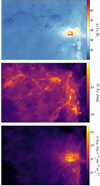 |
Fig. C.2 Maps of dust SED derived parameters at 30″ angular resolution. (a) Dust temperature, Td. (b) Visual extinction, AV. (c) FIR surface brightness (integrated from 40 to 500 µm). |
This fitting method works better on high S/N spectra. Thus, we only applied it to the main cloud velocity component (vLSR ≃10 km s−1) where S/N>5σ. Figure D.1 shows the anomalous HCN J = 1−0 spectrum observed (at by the IRAM 30m telescope toward the Horsehead PDR position δv ≃0.16 km s−1 resolution). This figure compares the expected HFS line strengths in the LTE and optically thin limit (green lines), the result of the LTE-HFS fit in CLASS (blue curve), and a non-LTE radiative transfer model (red curve, Goicoechea et al. 2022).
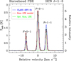 |
Fig. D.1 HCN J =1−0 HFS lines toward the Horsehead PDR. The right axis shows the normalized line intensity to make clear that the observed HFS emission differs from the optically thin LTE line ratios 1:5:3 (green lines). Red curves show the results of a non-LTE radiative transfer model including line overlaps (for details, see Sect. 5.1 in Goicoechea et al. 2022). Blue curves show the best LTE-HFS fit using CLASSfootnote 2. |
D.2 HCN J = 2−1 and 3−2 HFS line ratios
The HCN J = 2−1 transition has six HFS lines that blend into three lines with relative intensity ratios ~1:9:2 in the LTE and optically thin limit. The HCN J = 3−2 transition also has six HFS lines. Only the central ones are blended and cannot be spectrally resolved. This gives the impression of three lines with relative intensity ratios 1:25:1 in the LTE and optically thin limit (e.g., Ahrens et al. 2002; Loughnane et al. 2012). Here we term these three apparent components (blueshifted, central, and red-shifted) of the J = 2−1 and J = 3−2 rotational lines as “satellite(L),” “main,” and “satellite(R),” respectively. Table D.1 provides the entries used to construct Fig.11.
Appendix E HCN and HNC rotational diagrams
In Sect. 4.4, we analyzed multiple-J HCN and HNC line observations. Here we detail how we obtained the opacity corrected population diagrams. We took the HCN and HNC rotational spectroscopic parameters from CDMS (Endres et al. 2016, and references therein).
E.1 Estimation of line opacities:
To estimate the opacity of a given rotational transition HCN Ju → J1, we used the observed HCN/H13CN line ratio. We assumed that the H13CN Ju → Jı line is optically thin, that Trot is the same for the two isotopologues, and that HCN and H13CN Ju → J1 emit from the same gas volume (Goldsmith et al. 1984). Hence,
![${{{W_{{\rm{HCN}}}}} \over {{W_{{{\rm{H}}^{13}}{\rm{CN}}}}}} \approx {{1 - {e^{{\tau _{{\rm{HCN}}}}}}} \over {{\tau _{{\rm{HCN}}}}}}{{\left[ {^{12}{\rm{C}}} \right]} \over {\left[ {^{13}{\rm{C}}} \right]}},$](/articles/aa/full_html/2023/11/aa46598-23/aa46598-23-eq95.png) (E.1)
(E.1)
where τ is the line opacity, W is the integrated line intensity, and [12C]/[13C] is the isotopic ratio, around 60 in Orion (Langer & Penzias 1990).
The H13CN J=1−0 line is detected toward NGC 2024 cores, as well as toward the Horsehead PDR and Core positions in the higher sensitivity WHISPER survey (Gerin et al. 2009; Pety et al. 2012). We detect HCN and H13CN J = 2−1 toward several positions (#1, #2, #3, #4, #7, #8, HH-PDR and HH-Core). Table D.1 shows the estimated HCN J = 2−1 opacities following Eq. (E.1). We computed the opacities of the rotational lines J = 1−0 (for positions with no H13CN J = 1−0 detections), 3−2, and 4−3 as a function of J = 2−1 line opacity, as:
 (E.2)
(E.2)

where Trot is the rotational temperature, ul refers to the transition from the upper to lower level, and ∆vul is the linewidth. For simplicity, we assume a linewidth ratio ∆v2−1/∆vul = 1. For the fainter emitting positions, where we do not detect H13CN, we assume that the HCN emission is optically thin.
E.2 Opacity corrected population diagram
In order to determine Trot and the column density toward each observed position, we computed rotational diagrams assuming a single Trot(HCN) (Goldsmith & Langer 1999),
 (E.4)
(E.4)
where Nu is the level и population, Ntot is the total column density. We iteratively applied the opacity correction ( ) to the population diagram until a solution for Trot and N converged. For the first iteration we use eq. (E.4) and compute the line opacities from eq. (E.3). From the second iteration to convergence, we implement the opacity correction as
 (E.5)
(E.5)
The uncertainties are  , where ∆W is the uncertainty of the integrated intensity, ~20% of W. Figure E.1 shows a comparison between the optically thin (squares and dashed lines), and opacity-corrected HCN population diagrams (circles and straight lines), for positions #1, #2, and #4 in Fig. E.1a, and for positions #7, #8, and Core, in the Horsehead, in Fig. E.1b.
E.3 HNC rotational population diagrams
Table E.1 shows the rotational temperatures and column densities obtained from rotational diagrams constructed with the observed HNC J = 1−0 and J = 3−2 lines. This table also shows the estimated J = 1−0 line opacities toward positions with HNC and HN13C J = 1−0 detections (assuming that both emission lines steam from the same gas).
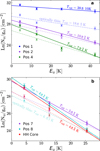 |
Fig. E.1 HCN rotational diagrams. (a) Opacity corrected (straight lines) population diagrams for positions #1, #2, #4. Lighter color dashed lines and squares show the optically thin population diagrams. (b) The same but for positions #7, #8, and the HH-Core. |
HNC excitation temperature and column densities obtained from rotational diagrams, as well as HNC J = 1−0 line opacities for positions in which we detected HN13C J = 1−0.
Appendix F Raster crossmap observation strategy
Because the telescope beam size changes with frequency, we split the observation of each position into a small raster crossmap of ~30” extent (the beam size in the 3 mm band). Figure F.1 shows the target positions. This way, the raster averaged spectra from the 2 and 1 mm bands (J = 2−1 and 3−2 lines), and to a lesser extend the 0.8 mm band ( J = 4−3), can directly be compared with the J = 1−0 observations.
Observed frequency ranges and telescope parameters
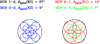 |
Fig. F.1 Pointing strategy of raster crossmaps designed to obtain multi frequency line observations at the ~30″ angular resolution of the Orion-B J = 1−0 maps. |
Appendix G Complementary figures and tables
In this section we provide figures (Figs. G.1 and G.2) with all detected HCN, HNC, H13CN, and HN13C line spectra toward the sampled of selected positions in Orion B (pointed observations). The following tables summarize their observed spectroscopic parameters: integrated line intensities, peak LSR velocity, line width and, peak temperature.
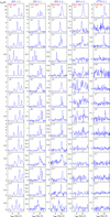 |
Fig. G.1 HCN J = 1−0 to J = 4−3, and H13CN J = 2−1 pointed observations. The velocity resolution is ∼0.5 km s−1. |
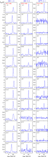 |
Fig. G.2 HNC J = 1−0 and J = 3−2, and HN13C J = 2−1 pointed observations. The velocity resolution is ∼0.5 km s−1. |
Line spectroscopie parameters obtained from Gaussian fits to the observed HCN lines.
Line spectroscopic parameters obtained from Gaussian fits to the observed HNC lines.
Line spectroscopic parameters obtained from Gaussian fits to the observed H13CN and HN13C lines.
References
- Abergel, A., Teyssier, D., Bernard, J. P., et al. 2003, A & A, 410, 577 [NASA ADS] [CrossRef] [EDP Sciences] [Google Scholar]
- Abt, H. A., & Levato, H. 1977, PASP, 89, 797 [CrossRef] [Google Scholar]
- Aguado, A., Roncero, O., Zanchet, A., Agúndez, M., & Cernicharo, J. 2017, ApJ, 838, 33 [Google Scholar]
- Ahrens, V., Lewen, F., Takano, S., et al. 2002, Z. Naturfor. A, 57, 669 [NASA ADS] [CrossRef] [Google Scholar]
- André, P., Men’shchikov, A., Bontemps, S., et al. 2010, A & A, 518, A102 [Google Scholar]
- Anthony-Twarog, B. J. 1982, AJ, 87, 1213 [NASA ADS] [CrossRef] [Google Scholar]
- Bally, J., Chambers, E., Guzman, V., et al. 2018, AJ, 155, 80 [Google Scholar]
- Barnes, P. J., Crutcher, R. M., Bieging, J. H., Storey, J. W. V., & Willner, S. P. 1989, ApJ, 342, 883 [NASA ADS] [CrossRef] [Google Scholar]
- Barnes, P. J., Ryder, S. D., O’Dougherty, S. N., et al. 2013, MNRAS, 432, 2231 [CrossRef] [Google Scholar]
- Barnes, A. T., Kauffmann, J., Bigiel, F., et al. 2020, MNRAS, 497, 1972 [NASA ADS] [CrossRef] [Google Scholar]
- Behrens, E., Mangum, J. G., Holdship, J., et al. 2022, ApJ, 939, 119 [NASA ADS] [CrossRef] [Google Scholar]
- Bik, A., Lenorzer, A., Kaper, L., et al. 2003, A & A, 404, 249 [NASA ADS] [CrossRef] [EDP Sciences] [Google Scholar]
- Bisbas, T. G., Schruba, A., & van Dishoeck, E. F. 2019, MNRAS, 485, 3097 [NASA ADS] [Google Scholar]
- Blake, G. A., Sutton, E. C., Masson, C. R., & Phillips, T. G. 1987, ApJ, 315, 621 [Google Scholar]
- Boger, G. I., & Sternberg, A. 2005, ApJ, 632, 302 [NASA ADS] [CrossRef] [Google Scholar]
- Boisse, P. 1990, A & A, 228, 483 [NASA ADS] [Google Scholar]
- Bowler, B. P., Waller, W. H., Megeath, S. T., Patten, B. M., & Tamura, M. 2009, AJ, 137, 3685 [NASA ADS] [CrossRef] [Google Scholar]
- Branham, J., Richard, L. 1995, Celest. Mech. Dyn. Astron., 61, 239 [NASA ADS] [CrossRef] [Google Scholar]
- Bublitz, J., Kastner, J. H., Santander-García, M., et al. 2019, A & A, 625, A101 [NASA ADS] [CrossRef] [EDP Sciences] [Google Scholar]
- Bublitz, J., Kastner, J. H., Hily-Blant, P., et al. 2022, A & A, 659, A197 [NASA ADS] [CrossRef] [EDP Sciences] [Google Scholar]
- Carilli, C. L., & Walter, F. 2013, ARA & A, 51, 105 [NASA ADS] [CrossRef] [Google Scholar]
- Caselli, P., Walmsley, C. M., Terzieva, R., & Herbst, E. 1998, ApJ, 499, 234 [Google Scholar]
- Cernicharo, J., Castets, A., Duvert, G., & Guilloteau, S. 1984a, A & A, 139, L13 [NASA ADS] [Google Scholar]
- Cernicharo, J., Guelin, M., & Askne, J. 1984b, A & A, 138, 371 [NASA ADS] [Google Scholar]
- Chandler, C. J., & Carlstrom, J. E. 1996, ApJ, 466, 338 [Google Scholar]
- Choi, M., Kang, M., & Lee, J.-E. 2015, AJ, 150, 29 [NASA ADS] [CrossRef] [Google Scholar]
- Clark, F. O., Buhl, D., & Snyder, L. E. 1974, ApJ, 190, 545 [NASA ADS] [CrossRef] [Google Scholar]
- Dame, T. M., & Lada, C. J. 2023, ApJ, 944, 197 [NASA ADS] [CrossRef] [Google Scholar]
- Daniel, F., & Cernicharo, J. 2008, A & A, 488, 1237 [CrossRef] [EDP Sciences] [Google Scholar]
- Denis-Alpizar, O., Stoecklin, T., Dutrey, A., & Guilloteau, S. 2020, MNRAS, 497, 4276 [Google Scholar]
- Dickinson, A. S., Phillips, T. G., Goldsmith, P. F., Percival, I. C., & Richards, D. 1977, A & A, 54, 645 [Google Scholar]
- Elmegreen, B. G. 2002, ApJ, 577, 206 [CrossRef] [Google Scholar]
- Emprechtinger, M., Wiedner, M. C., Simon, R., et al. 2009, A & A, 496, 731 [NASA ADS] [CrossRef] [EDP Sciences] [Google Scholar]
- Endres, C. P., Schlemmer, S., Schilke, P., Stutzki, J., & Müller, H. S. 2016, J. Mol. Spectrosc., 327, 955, new Visions of Spectroscopic Databases, Volume II [NASA ADS] [CrossRef] [Google Scholar]
- Evans, I., Neal, J. 1999, ARA & A, 37, 311 [NASA ADS] [CrossRef] [Google Scholar]
- Evans, I., Neal, J., Kim, K.-T., Wu, J., et al. 2020, ApJ, 894, 103 [NASA ADS] [CrossRef] [Google Scholar]
- Falgarone, E., Phillips, T. G., & Walker, C. K. 1991, ApJ, 378, 186 [NASA ADS] [CrossRef] [Google Scholar]
- Faure, A., & Lique, F. 2012, MNRAS, 425, 740 [NASA ADS] [CrossRef] [Google Scholar]
- Faure, A., Tennyson, J., Varambhia, H. N., et al. 2007a, in SF2A-2007: Proceedings of the Annual meeting of the French Society of Astronomy and Astrophysics, eds. J. Bouvier, A. Chalabaev, & C. Charbonnel, 244 [Google Scholar]
- Faure, A., Varambhia, H. N., Stoecklin, T., & Tennyson, J. 2007b, MNRAS, 382, 840 [Google Scholar]
- Faure, A., Tennyson, J., Kokoouline, V., & Greene, C. H. 2009, J. Phys. Conf. Ser., 192, 012016 [CrossRef] [Google Scholar]
- Fuller, G. A., Myers, P. C., Welch, W. J., et al. 1991, ApJ, 376, 135 [NASA ADS] [CrossRef] [Google Scholar]
- Gallagher, M. J., Leroy, A. K., Bigiel, F., et al. 2018, ApJ, 868, L38 [CrossRef] [Google Scholar]
- Gao, Y., & Solomon, P. M. 2004a, ApJS, 152, 63 [Google Scholar]
- Gao, Y., & Solomon, P. M. 2004b, ApJ, 606, 271 [NASA ADS] [CrossRef] [Google Scholar]
- Gao, Y., Carilli, C. L., Solomon, P. M., & Vanden Bout, P. A. 2007, ApJ, 660, L93 [NASA ADS] [CrossRef] [Google Scholar]
- García-Burillo, S., Usero, A., Alonso-Herrero, A., et al. 2012, A & A, 539, A8 [CrossRef] [EDP Sciences] [Google Scholar]
- Gaudel, M., Orkisz, J. H., Gerin, M., et al. 2023, A & A, 670, A59 [NASA ADS] [CrossRef] [EDP Sciences] [Google Scholar]
- Gaume, R. A., Johnston, K. J., & Wilson, T. L. 1992, ApJ, 388, 489 [NASA ADS] [CrossRef] [Google Scholar]
- Gerin, M., Goicoechea, J. R., Pety, J., & Hily-Blant, P. 2009, A & A, 494, 977 [CrossRef] [EDP Sciences] [Google Scholar]
- Giannini, T., Nisini, B., Lorenzetti, D., et al. 2000, A & A, 358, 310 [NASA ADS] [Google Scholar]
- Godard, B., Falgarone, E., Gerin, M., Hily-Blant, P., & de Luca, M. 2010, A & A, 520, A20 [NASA ADS] [CrossRef] [EDP Sciences] [Google Scholar]
- Goicoechea, J. R., & Cuadrado, S. 2021, A & A, 647, A7 [Google Scholar]
- Goicoechea, J. R., & Le Bourlot, J. 2007, A & A, 467, 1 [NASA ADS] [CrossRef] [EDP Sciences] [Google Scholar]
- Goicoechea, J. R., & Roncero, O. 2022, A & A, 664, A190 [NASA ADS] [CrossRef] [EDP Sciences] [Google Scholar]
- Goicoechea, J. R., Pety, J., Gerin, M., Hily-Blant, P., & Le Bourlot, J. 2009, A & A, 498, 771 [NASA ADS] [CrossRef] [EDP Sciences] [Google Scholar]
- Goicoechea, J. R., Pety, J., Cuadrado, S., et al. 2016, Nature, 537, 207 [Google Scholar]
- Goicoechea, J. R., Lique, F., & Santa-Maria, M. G. 2022, A & A, 658, A28 [NASA ADS] [CrossRef] [EDP Sciences] [Google Scholar]
- Goldsmith, P. F., & Kauffmann, J. 2017, ApJ, 841, 25 [Google Scholar]
- Goldsmith, P. F., & Langer, W. D. 1999, ApJ, 517, 209 [Google Scholar]
- Goldsmith, P. F., Snell, R. L., Hemeon-Heyer, M., & Langer, W. D. 1984, ApJ, 286, 599 [NASA ADS] [CrossRef] [Google Scholar]
- Gonzalez-Alfonso, E., & Cernicharo, J. 1993, A & A, 279, 506 [NASA ADS] [Google Scholar]
- Gottlieb, C. A., Lada, C. J., Gottlieb, E. W., Lilley, A. E., & Litvak, M. M. 1975, ApJ, 202, 655 [NASA ADS] [CrossRef] [Google Scholar]
- Graninger, D. M., Herbst, E., Öberg, K. I., & Vasyunin, A. I. 2014, ApJ, 787, 74 [Google Scholar]
- Guelin, M., Langer, W. D., & Wilson, R. W. 1982, A & A, 107, 107 [NASA ADS] [Google Scholar]
- Guilloteau, S., & Baudry, A. 1981, A & A, 97, 213 [NASA ADS] [Google Scholar]
- Habart, E., Abergel, A., Walmsley, C. M., Teyssier, D., & Pety, J. 2005, A & A, 437, 177 [NASA ADS] [CrossRef] [EDP Sciences] [Google Scholar]
- Habart, E., Le Gal, R., Alvarez, C., et al. 2023a, A & A, 673, A149 [NASA ADS] [CrossRef] [EDP Sciences] [Google Scholar]
- Habart, E., Peeters, E., Berne, O., et al. 2023b, A & A, in press, https://doi.org/10.1051/0004-6361/202346747 [Google Scholar]
- Hacar, A., Bosman, A. D., & van Dishoeck, E. F. 2020, A & A, 635, A4 [NASA ADS] [CrossRef] [EDP Sciences] [Google Scholar]
- Heays, A. N., Bosman, A. D., & van Dishoeck, E. F. 2017, A & A, 602, A105 [NASA ADS] [CrossRef] [EDP Sciences] [Google Scholar]
- Helfer, T. T., & Blitz, L. 1997, ApJ, 478, 233 [NASA ADS] [CrossRef] [Google Scholar]
- Herbst, E., Terzieva, R., & Talbi, D. 2000, MNRAS, 311, 869 [NASA ADS] [CrossRef] [Google Scholar]
- Hernández Vera, M., Lique, F., Dumouchel, F., Hily-Blant, P., & Faure, A. 2017, MNRAS, 468, 1084 [Google Scholar]
- Hily-Blant, P., Walmsley, M., Pineau Des Forêts, G., & Flower, D. 2010, A & A, 513, A41 [NASA ADS] [CrossRef] [EDP Sciences] [Google Scholar]
- Hollenbach, D. J., Takahashi, T., & Tielens, A. G. G. M. 1991, ApJ, 377, 192 [NASA ADS] [CrossRef] [Google Scholar]
- Hollenbach, D. J., & Tielens, A. G. G. M. 1999, Rev. Mod. Phys., 71, 173 [Google Scholar]
- Ikeda, M., Oka, T., Tatematsu, K., Sekimoto, Y., & Yamamoto, S. 2002, ApJS, 139, 467 [NASA ADS] [CrossRef] [Google Scholar]
- Indriolo, N., Neufeld, D. A., Gerin, M., et al. 2015, ApJ, 800, 40 [NASA ADS] [CrossRef] [Google Scholar]
- Jiménez-Donaire, M. J., Bigiel, F., Leroy, A. K., et al. 2017, MNRAS, 466, 49 [CrossRef] [Google Scholar]
- Jiménez-Donaire, M. J., Bigiel, F., Leroy, A. K., et al. 2019, ApJ, 880, 127 [CrossRef] [Google Scholar]
- Johnson, C. T., Burke, P. G., & Kingston, A. E. 1987, J. Phys. B At. Mol. Phys., 20, 2553 [CrossRef] [Google Scholar]
- Kaufman, M. J., Wolfire, M. G., Hollenbach, D. J., & Luhman, M. L. 1999, ApJ, 527, 795 [Google Scholar]
- Kauffmann, J., Goldsmith, P. F., Melnick, G., et al. 2017, A & A, 605, A5 [Google Scholar]
- Kennicutt, R. C. J. 1998a, ARA & A, 36, 189 [NASA ADS] [CrossRef] [Google Scholar]
- Kennicutt, R. C. J., 1998b, ApJ, 498, 541 [NASA ADS] [CrossRef] [Google Scholar]
- Kennicutt, R. C., & Evans, N. J. 2012, ARA & A, 50, 531 [NASA ADS] [CrossRef] [Google Scholar]
- Keto, E., & Rybicki, G. 2010, ApJ, 716, 1315 [NASA ADS] [CrossRef] [Google Scholar]
- Könyves, V., André, P., Arzoumanian, D., et al. 2020, A & A, 635, A34 [CrossRef] [EDP Sciences] [Google Scholar]
- Krumholz, M. R., & Thompson, T. A. 2007, ApJ, 669, 289 [NASA ADS] [CrossRef] [Google Scholar]
- Kwan, J., & Scoville, N. 1975, ApJ, 195, L85 [NASA ADS] [CrossRef] [Google Scholar]
- Lada, E. A. 1992, ApJ, 393, L25 [NASA ADS] [CrossRef] [Google Scholar]
- Lada, C. J., & Lada, E. A. 2003, ARA & A, 41, 57 [NASA ADS] [CrossRef] [Google Scholar]
- Lada, E. A., Evans, I., Neal, J. & Falgarone, E. 1997, ApJ, 488, 286 [NASA ADS] [CrossRef] [Google Scholar]
- Lada, C. J., Lombardi, M., & Alves, J. F. 2010, ApJ, 724, 687 [Google Scholar]
- Langer, W. D., & Penzias, A. A. 1990, ApJ, 357, 477 [Google Scholar]
- Langer, W. D., Wilson, R. W., Henry, P. S., & Guelin, M. 1978, ApJ, 225, L139 [NASA ADS] [CrossRef] [Google Scholar]
- Le Petit, F., Nehmé, C., Le Bourlot, J., & Roueff, E. 2006, ApJS, 164, 506 [NASA ADS] [CrossRef] [Google Scholar]
- Lim, J., Dinh-V-Trung, Vrtilek, J., David, L. P., & Forman, W. 2017, ApJ, 850, 31 [CrossRef] [Google Scholar]
- Lin, M. C., Yinsheng, H., & Melius, C. 1992, Int. J. Chem. Kinet., 24, 1103 [CrossRef] [Google Scholar]
- Liszt, H. S. 2012, A & A, 538, A27 [NASA ADS] [CrossRef] [EDP Sciences] [Google Scholar]
- Liszt, H., & Lucas, R. 2001, A & A, 370, 576 [NASA ADS] [CrossRef] [EDP Sciences] [Google Scholar]
- Liszt, H. S., & Pety, J. 2016, ApJ, 823, 124 [NASA ADS] [CrossRef] [Google Scholar]
- Loison, J. C., & Hickson, K. M. 2015, Chem. Phys. Lett., 635, 174 [NASA ADS] [CrossRef] [Google Scholar]
- Loison, J.-C., Wakelam, V., & Hickson, K. M. 2014, MNRAS, 443, 398 [Google Scholar]
- Lombardi, M., Bouy, H., Alves, J., & Lada, C. J. 2014, A & A, 566, A45 [NASA ADS] [CrossRef] [EDP Sciences] [Google Scholar]
- Loughnane, R. M., Redman, M. P., Thompson, M. A., et al. 2012, MNRAS, 420, 1367 [NASA ADS] [CrossRef] [Google Scholar]
- Madore, B. F. 1977, MNRAS, 178, 1 [NASA ADS] [CrossRef] [Google Scholar]
- Magalhães, V. S., Hily-Blant, P., Faure, A., Hernandez-Vera, M., & Lique, F. 2018, A & A, 615, A52 [CrossRef] [EDP Sciences] [Google Scholar]
- McDowell, R. S. 1988, J. Chem. Phys., 88, 356 [NASA ADS] [CrossRef] [Google Scholar]
- Megeath, S. T., Gutermuth, R., Muzerolle, J., et al. 2016, AJ, 151, 5 [Google Scholar]
- Meyer, M. R., Flaherty, K., Levine, J. L., et al. 2008, in Handbook of Star Forming Regions, 4, ed. B. Reipurth, 662 [NASA ADS] [Google Scholar]
- Mezger, P. G., Chini, R., Kreysa, E., Wink, J. E., & Salter, C. J. 1988, A & A, 191, 44 [NASA ADS] [Google Scholar]
- Miettinen, O., Harju, J., Haikala, L. K., Kainulainen, J., & Johansson, L. E. B. 2009, A & A, 500, 845 [NASA ADS] [CrossRef] [EDP Sciences] [Google Scholar]
- Miettinen, O., Harju, J., Haikala, L. K., & Juvela, M. 2010, A & A, 524, A91 [NASA ADS] [CrossRef] [EDP Sciences] [Google Scholar]
- Mitchell, G. F. 1984, ApJS, 54, 81 [Google Scholar]
- Narayanan, D., Cox, T. J., Shirley, Y., et al. 2008, ApJ, 684, 996 [NASA ADS] [CrossRef] [Google Scholar]
- Neumann, L., Gallagher, M. J., Bigiel, F., et al. 2023, MNRAS, 521, 3348 [NASA ADS] [CrossRef] [Google Scholar]
- O’Konski, C. T., & Ha, T.-K. 1968, J. Chem. Phys., 49, 5354 [CrossRef] [Google Scholar]
- Orkisz, J. H., Peretto, N., Pety, J., et al. 2019, A & A, 624, A113 [CrossRef] [EDP Sciences] [Google Scholar]
- Pabst, C. H. M., Goicoechea, J. R., Teyssier, D., et al. 2017, A & A, 606, A29 [NASA ADS] [CrossRef] [EDP Sciences] [Google Scholar]
- Pabst, C. H. M., Hacar, A., Goicoechea, J. R., et al. 2021, A & A, 651, A111 [NASA ADS] [CrossRef] [EDP Sciences] [Google Scholar]
- Papadopoulos, P. P., Zhang, Z.-Y., Xilouris, E. M., et al. 2014, ApJ, 788, 153 [CrossRef] [Google Scholar]
- Patra, S., Evans, Neal J., I., Kim, K.-T., et al. 2022, AJ, 164, 129 [NASA ADS] [CrossRef] [Google Scholar]
- Petrie, S. 2002, J. Phys. Chem. A, 106, 11181 [CrossRef] [Google Scholar]
- Pety, J., Goicoechea, J. R., Hily-Blant, P., Gerin, M., & Teyssier, D. 2007, A & A, 464, L41 [NASA ADS] [CrossRef] [EDP Sciences] [Google Scholar]
- Pety, J., Gratier, P., Guzmán, V., et al. 2012, A & A, 548, A68 [NASA ADS] [CrossRef] [EDP Sciences] [Google Scholar]
- Pety, J., Guzmán, V. V., Orkisz, J. H., et al. 2017, A & A, 599, A98 [CrossRef] [EDP Sciences] [Google Scholar]
- Philipp, S. D., Lis, D. C., Güsten, R., et al. 2006, A & A, 454, 213 [NASA ADS] [CrossRef] [EDP Sciences] [Google Scholar]
- Pickering, E. C. 1908, Ann. Harvard Coll. Observ., 60, 147 [NASA ADS] [Google Scholar]
- Ren, Z., & Li, D. 2016, ApJ, 824, 52 [NASA ADS] [CrossRef] [Google Scholar]
- Rezaei Kh., S., Bailer-Jones, C. A. L., Soler, J. D., & Zari, E. 2020, A & A, 643, A151 [CrossRef] [EDP Sciences] [Google Scholar]
- Rosolowsky, E., Pineda, J. E., & Gao, Y. 2011, MNRAS, 415, 1977 [NASA ADS] [CrossRef] [Google Scholar]
- Rybak, M., Hodge, J. A., Greve, T. R., et al. 2022, A & A, 667, A70 [NASA ADS] [CrossRef] [EDP Sciences] [Google Scholar]
- Sánchez-García, M., García-Burillo, S., Pereira-Santaella, M., et al. 2022, A & A, 660, A83 [CrossRef] [EDP Sciences] [Google Scholar]
- Sandell, G., Mookerjea, B., Güsten, R., et al. 2015, A & A, 578, A41 [NASA ADS] [CrossRef] [EDP Sciences] [Google Scholar]
- Sanders, D. B., & Mirabel, I. F. 1996, ARA & A, 34, 749 [NASA ADS] [CrossRef] [Google Scholar]
- Santa-Maria, M. G., Goicoechea, J. R., Etxaluze, M., Cernicharo, J., & Cuadrado, S. 2021, A & A, 649, A32 [NASA ADS] [CrossRef] [EDP Sciences] [Google Scholar]
- Schaefer, G. H., Hummel, C. A., Gies, D. R., et al. 2016, AJ, 152, 213 [NASA ADS] [CrossRef] [Google Scholar]
- Schilke, P., Walmsley, C. M., Pineau Des Forets, G., et al. 1992, A & A, 256, 595 [NASA ADS] [Google Scholar]
- Schmidt, M. 1959, ApJ, 129, 243 [NASA ADS] [CrossRef] [Google Scholar]
- Schmidt, M. 1963, ApJ, 137, 758 [Google Scholar]
- Schneider, N., André, P., Könyves, V., et al. 2013, ApJ, 766, L17 [NASA ADS] [CrossRef] [Google Scholar]
- Schroder, K., Staemmler, V., Smith, M. D., Flower, D. R., & Jaquet, R. 1991, J. Phys. B At. Mol. Phys., 24, 2487 [NASA ADS] [CrossRef] [Google Scholar]
- Semaniak, J., Minaev, B. F., Derkatch, A. M., et al. 2001, ApJS, 135, 275 [NASA ADS] [CrossRef] [Google Scholar]
- Shetty, R., Kelly, B. C., & Bigiel, F. 2013, MNRAS, 430, 288 [NASA ADS] [CrossRef] [Google Scholar]
- Shetty, R., Clark, P. C., & Klessen, R. S. 2014a, MNRAS, 442, 2208 [NASA ADS] [CrossRef] [Google Scholar]
- Shetty, R., Kelly, B. C., Rahman, N., et al. 2014b, MNRAS, 437, L61 [NASA ADS] [CrossRef] [Google Scholar]
- Shimajiri, Y., André, P., Braine, J., et al. 2017, A & A, 604, A74 [NASA ADS] [CrossRef] [EDP Sciences] [Google Scholar]
- Shirley, Y. L. 2015, PASP, 127, 299 [Google Scholar]
- Shirley, Y. L., Wu, J., Shane Bussmann, R., & Wootten, A. 2008, in ASP Conf. Ser., 387, Massive Star Formation: Observations Confront Theory, eds. H. Beuther, H. Linz, & T. Henning, 401 [Google Scholar]
- Sofia, U. J., Lauroesch, J. T., Meyer, D. M., & Cartledge, S. I. B. 2004, ApJ, 605, 272 [NASA ADS] [CrossRef] [Google Scholar]
- Sohn, J., Lee, C. W., Park, Y.-S., et al. 2007, ApJ, 664, 928 [NASA ADS] [CrossRef] [Google Scholar]
- Solomon, P. M., Downes, D., & Radford, S. J. E. 1992, ApJ, 387, L55 [NASA ADS] [CrossRef] [Google Scholar]
- Spaans, M. 1996, A & A, 307, 271 [Google Scholar]
- Stephens, I. W., Jackson, J. M., Whitaker, J. S., et al. 2016, ApJ, 824, 29 [NASA ADS] [CrossRef] [Google Scholar]
- Sternberg, A., & Dalgarno, A. 1995, ApJS, 99, 565 [NASA ADS] [CrossRef] [Google Scholar]
- Stutzki, J., Bensch, F., Heithausen, A., Ossenkopf, V., & Zielinsky, M. 1998, A & A, 336, 697 [NASA ADS] [Google Scholar]
- Sumathi, R., & Nguyen, M. T. 1998, J. Phys. Chem. A, 102, 8013 [NASA ADS] [CrossRef] [Google Scholar]
- Tafalla, M., Usero, A., & Hacar, A. 2021, A & A, 646, A97 [NASA ADS] [CrossRef] [EDP Sciences] [Google Scholar]
- Talbi, D., Ellinger, Y., & Herbst, E. 1996, A & A, 314, 688 [Google Scholar]
- Turner, B. E., Pirogov, L., & Minh, Y. C. 1997, ApJ, 483, 235 [CrossRef] [Google Scholar]
- Usero, A., Leroy, A. K., Walter, F., et al. 2015, AJ, 150, 115 [Google Scholar]
- Virtanen, P., Gommers, R., Oliphant, T. E., et al. 2020, Nat. Methods, 17, 261 [Google Scholar]
- Walmsley, C. M., Churchwell, E., Nash, A., & Fitzpatrick, E. 1982, ApJ, 258, L75 [NASA ADS] [CrossRef] [Google Scholar]
- Walter, F. M., Sherry, W. H., Wolk, S. J., & Adams, N. R. 2008, in Handbook of Star Forming Regions, Volume I, 732, ed. B. Reipurth, 732 [Google Scholar]
- Wannier, P. G., Encrenaz, P. J., Wilson, R. W., & Penzias, A. A. 1974, ApJ, 190, L77 [NASA ADS] [CrossRef] [Google Scholar]
- Wu, J., Evans, I., Neal, J., Gao, Y., et al. 2005, ApJ, 635, L173 [NASA ADS] [CrossRef] [Google Scholar]
- Wu, J., Evans, I., Neal, J., Shirley, Y. L., & Knez, C. 2010, ApJS, 188, 313 [NASA ADS] [CrossRef] [Google Scholar]
- Yamada, M., Wada, K., & Tomisaka, K. 2007, ApJ, 671, 73 [NASA ADS] [CrossRef] [Google Scholar]
- Yang, B., Stancil, P. C., Balakrishnan, N., & Forrey, R. C. 2010, ApJ, 718, 1062 [Google Scholar]
- Young Owl, R. C., Meixner, M. M., Wolfire, M., Tielens, A. G. G. M., & Tauber, J. 2000, ApJ, 540, 886 [Google Scholar]
- Zucker, C., Speagle, J. S., Schlafly, E. F., et al. 2019, ApJ, 879, 125 [NASA ADS] [CrossRef] [Google Scholar]
- Zymak, I., Hejduk, M., Mulin, D., et al. 2013, ApJ, 768, 86 [NASA ADS] [CrossRef] [Google Scholar]
Interferometric observations of the σ Ori system provides a distance of ~388 pc (Schaefer et al. 2016). Recent determinations using Gaia also estimate ~400 pc (e.g., Zucker et al. 2019; Rezaei Kh. et al. 2020).
Section 6.4 discusses the relation between these lines and IFIR.
This value is higher than the line intensity of the average HCN J =1−0 spectrum over the full mapped area (see Table 4), thus including emission free pixels. The mean and median W(HCN J = 1−0) intensity values computed considering pixels with CO J = 1−0 detections above 3e are 1.0 and 0.7 K km s−1, respectively.
In these 1D PDR models, the cloud depth or shielding (AV in mag of visual extinction) refers to the extinction normal to the cloud surface and parallel to the FUV illumination direction. In general, this extinction is different from AV determined from observations and the dust SED along a given line of sight. Only for a face-on cloud (with the illuminating stars in the observed line of sight) both magnitudes are equivalent.
Appendix C.2 details how we determine the gas mass.
Using the Scipy-odr package (Branham 1995; Virtanen et al. 2020). https://docs.scipy.org/doc/scipy/reference/odr.html
The total FIR luminosity in the mapped region of Orion B (~ 250 pc2) is LFIR = 1.5 × 10⁵ L⊙ (or ΣFIR = 6 × 10² L⊙ pc−2). Using the extragalactic scalings (e.g., Kennicutt 1998a), these FIR luminosities translate into a SFR of 2.6 × 10⁻⁵ M⊙ yr−1, which is nearly an order of magnitude lower than the SFR estimated by counting young stellar objects (YSOs), 1.6 × 10⁻⁴ M⊙ yr−1 (Lada et al. 2010). Pabst et al. (2021) find a similar result in Orion A, namely that SFR(FIR) < SFR(YSOs).
Discovered by Williamina Fleming (Pickering 1908).
The HGBS data can be found at http://www.herschel.fr/cea/star-formation/en/Phocea/Vie_des_labos/Ast/ast_visu.php?id_ast=66
All Tables
Spectroscopic parameters of the lines studied in this work (from Endres et al. 2016, and references therein), critical densities for collisions with p-H2 and electrons at 20 K (if LTE prevails, 99.82% of H2 is in para form), and critical fractional abundance of electrons (see text).
HCN J = 1−0 HFS line intensity ratios, W(HCN J = 2−1)/W(HCN J =1−0) and W(HCN J = 3−2)/W(HCN J =1−0) line intensity ratios, and parameters derived from rotational population diagrams, computed in Appendix E, toward a sample of representative cloud positions.
HNC rotational temperatures, HCN/HNC column density, and line intensity ratios toward selected positions in Orion B.
HNC excitation temperature and column densities obtained from rotational diagrams, as well as HNC J = 1−0 line opacities for positions in which we detected HN13C J = 1−0.
Line spectroscopie parameters obtained from Gaussian fits to the observed HCN lines.
Line spectroscopic parameters obtained from Gaussian fits to the observed HNC lines.
Line spectroscopic parameters obtained from Gaussian fits to the observed H13CN and HN13C lines.
All Figures
|
Fig. 1 Composite image of the ~5 deg2 area mapped in Orion B. Red color represents the PACS 70 μm emission tracing FUV-illuminated extended warm dust. Green color represents the cloud depth in magnitudes of visual extinction, AV ∝ N(H2). Blue color represents the HCN J = 1−0 line intensity. We note that outside the main filaments most of the HCN J =1−0 emission is at AV < 4 mag. |
| In the text | |
|
Fig. 2 Maps of Orion B in different tracers. (a) Visual extinction AV, (b) Approximate FUV field, |
| In the text | |
|
Fig. 3 Selection of HCN J = 1−0 to 4−3, and HNC J = 3−2 line detections toward representative cloud environments in OrionB. Red lines show the expected relative HFS line intensities in the LTE and optically thin limit. |
| In the text | |
|
Fig. 4 Distribution of 12CO, HCN, HCO+, HNC J = 1−0, and [C I] 492 GHz line intensities as a function of AV. The dashed red lines show the running median (median values of the line intensity within equally spaced log AV bins). Error bars show the line intensity dispersion. We note that the 5σ error of AV is ≃0.8 mag. Thus, one cannot trust any trend below this threshold. |
| In the text | |
|
Fig. 5 Line emission properties as a function of AV. (a) Fractions (in %) of line luminosities emitted in each Ay mask. (b) Typical (the mode) line intensity in each AV mask. (c) Cumulative line luminosity. |
| In the text | |
|
Fig. 6 Line intensity ratio maps. Contours show AV = 4, 6, 8, and 15 mag. |
| In the text | |
|
Fig. 7 Spatial distribution of Tex(HCN J = 1−0) and N(HCN) estimated from LTE-HFS fits, and maps of HCN J = 1−0 HFS intensity ratios. (a) Tex(HCN J = 1−0). (b) Opacity-corrected column densities N(HCN). (c) and (d) R02 and R12 (white color corresponds to non-anomalous ratios). |
| In the text | |
|
Fig. 8 Histograms of HCN J =1−0 HFS (a) Line intensity ratios, and (b) Line-width ratios observed in OrionB. R02 stands for W(F = 0−1)/W(F = 2−1) and R12 stands for W(F = 1–1)/W(F = 2−1). The red curve in panel (a) shows the expected LTE ratios as line opacities increase. The red star marks the non-anomalous ratios in the optically thin limit τ → 0 (1σ is the standard deviation relative to the mean line ratios). |
| In the text | |
|
Fig. 9 Comparison of observed W(HCN J = 1−0) intensities in Orion B and predictions from nonlocal and non-LTE radiative transfer models including line overlap for (a) N(HCN) = 1013 cm−2 and (b) N(HCN) = 1014 cm−2. The continuous curves show model results for Tk = 60, 30, and 10 K (red, green, and blue curves, respectively), different ionization fractions: χe = 0 (continuous curves), χe = 2×10⁻⁵ (dashed curves), and χe = 10−4 (dotted curves). The pink and orange horizontal line mark the mean and median values of W(HCN J = 1−0). The pink shaded area represents the standard deviation (1er) relative to the mean detected W(HCN J = 1−0) intensities in Orion B (at 30″). Positions in the pink area account for -70% of the total LHCN 1−0 in the map. The right panels show an histogram with the distribution of W(HCN J =1−0) detections in individual map pixels. |
| In the text | |
|
Fig. 10 W(HCN J = 1−0) (red curves) and Tex (HCN J = 1−0 F = 2−1) (blue curves) predicted by non-LTE radiative transfer models, appropriate to extended and translucent gas, as a function of electron abundance. The vertical pink shaded area intersects the typical W(HCN J = 1−0) = 1 K km s−1 intensity level ( ± 20%). |
| In the text | |
|
Fig. 11 HCN J = 2−1 and J = 3−2 HFS intensity ratios satellite(R)/main versus satellite(B)/main (see Sect. 4.4 for their definition) in LTE and as line opacities increase. Blue and red dots show the observed HFS line ratios toward the representative positions (see Table D.1). |
| In the text | |
|
Fig. 12 2D histogram of the observed HCN/HNC J = 1–0 line intensity ratio as a function of G′0 in the Orion B map. The dashed black curve shows the running median. The error bars show the standard deviation. |
| In the text | |
|
Fig. 13 Constant density gas-phase PDR models with G0 = 100 and nH = 5 × 103 cm−3 (left) and 5 × 104 cm−3 (right). These models adopt Eb = 1200 K for Reaction (8). Upper panels in (a) and (b): dashed curves show the depth-dependent column density ratios of selected species (left y-axis). The blue continuous curves in the upper panels of (a) and (b) show the HCN/HNC column density ratio adopting Eb = 200 K. Green continuous curves show the temperature structure as a function of AV (right y-axis). Lower panels in (a) and (b): abundance profiles with respect to H nuclei. (c) and (d): Contribution (in percent) of the main formation and destruction reactions for HCN (continuous curves) and HNC (dashed curves). |
| In the text | |
|
Fig. 14 Dominant chemical reactions in FUV-illuminated gas. |
| In the text | |
|
Fig. 15 Dominant chemical reactions in FUV-shielded gas. |
| In the text | |
|
Fig. 16 2D histograms. (a) Visual extinction AV as a function of the HCN/CO J =1–0 integrated intensity ratio (from maps at 120″ resolution). Dashed red, yellow, green, and blue horizontal lines are the visual extinction values 1, 4, 8, and 15 mag, respectively. Above each line, we show the percentage of the total HCN J = 1–0 luminosity that comes from the different AV ranges. (b), (c), and (d) 2D histogram of the observed [C I] 492 GHz/CO J =1–0 line intensity ratio (in units of K km s−1) as function of the observed HCN/CO J =1–0 line ratio for all AV, for AV < 3 mag, and for AV > 3 mag. The dashed black curve shows the running median. Error bars show the standard deviation in the x-axis. |
| In the text | |
|
Fig. 17 30″-resolution view of the Horse-head. (a) [C II] 158 µm (Pabst et al. 2017) and (b) [C I] 492 GHz (Philipp et al. 2006) integrated line intensity maps (from 7 to 18 km s−1). (c) R = HCN/CO intensity ratio and (d) HCN J = 1−0 line intensity maps. Contours on [C II] 158 µm map: HCN/CO ratio (R = 0.06 and 0.12). Contours on [C I] 492 GHz map: HCN J =1−0 surface brightness (W = 2.7, 4.5, and 6 K km s−1). |
| In the text | |
|
Fig. 18 2D histograms of the 12CO, HCN, HCO+, HNC, J = 1–0, and [C I]3P1 – 3P0 line intensities as a function of FIR intensity in Orion B (from maps at 120″ resolution). The dashed red lines show the running median (median values of the integrated intensity within equally spaced log IFIR bins). The error bars show their dispersion. Black lines (and associated text) show a linear fit (orthogonal regression in log(y)-log(x)) to all observed positions in each map. Magenta lines and blue lines show a linear fit to a range of IFIR <6 × 10⁻³ erg s−1 cm−2 sr−1 and (0.4–7.7) erg s−1 cm−2 sr−1, respectively. We note that in each plot the number of line detections is different. |
| In the text | |
|
Fig. B.1 2D histograms showing the line intensity ratios HCN/CO, HCN/HNC, HCN/HCO+ J = 1–0, and [C I] 492 GHz/CO J = 1–0 with respect to the visual extinction AV. The dashed red line marks the running median. The error bars mark the standard deviation. The dashed black line marks the intensity ratio equal to one. |
| In the text | |
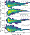 |
Fig. B.2 Same as Fig. B.1 but as a function of IFIR. |
| In the text | |
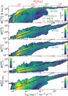 |
Fig. B.3 Same as Fig. 18 but showing the exponents |
| In the text | |
|
Fig. C.1 Compositing geometry in the NGC 2024 region between data from Lombardi et al. (2014) and Könyves et al. (2020), for column density (left) and dust temperature (right). The outer contour is the one in which the compositing is executed. The “selection area” over which the K20 datasets are rescaled to match the L14 ones corresponds to the outer contour minus the inner, hashed area (affected by the artifact in L14 and masked out). The full maps corresponding to these zoom-ins can be found in Fig. C.2 |
| In the text | |
|
Fig. C.2 Maps of dust SED derived parameters at 30″ angular resolution. (a) Dust temperature, Td. (b) Visual extinction, AV. (c) FIR surface brightness (integrated from 40 to 500 µm). |
| In the text | |
|
Fig. D.1 HCN J =1−0 HFS lines toward the Horsehead PDR. The right axis shows the normalized line intensity to make clear that the observed HFS emission differs from the optically thin LTE line ratios 1:5:3 (green lines). Red curves show the results of a non-LTE radiative transfer model including line overlaps (for details, see Sect. 5.1 in Goicoechea et al. 2022). Blue curves show the best LTE-HFS fit using CLASSfootnote 2. |
| In the text | |
|
Fig. E.1 HCN rotational diagrams. (a) Opacity corrected (straight lines) population diagrams for positions #1, #2, #4. Lighter color dashed lines and squares show the optically thin population diagrams. (b) The same but for positions #7, #8, and the HH-Core. |
| In the text | |
|
Fig. F.1 Pointing strategy of raster crossmaps designed to obtain multi frequency line observations at the ~30″ angular resolution of the Orion-B J = 1−0 maps. |
| In the text | |
|
Fig. G.1 HCN J = 1−0 to J = 4−3, and H13CN J = 2−1 pointed observations. The velocity resolution is ∼0.5 km s−1. |
| In the text | |
|
Fig. G.2 HNC J = 1−0 and J = 3−2, and HN13C J = 2−1 pointed observations. The velocity resolution is ∼0.5 km s−1. |
| In the text | |
Current usage metrics show cumulative count of Article Views (full-text article views including HTML views, PDF and ePub downloads, according to the available data) and Abstracts Views on Vision4Press platform.
Data correspond to usage on the plateform after 2015. The current usage metrics is available 48-96 hours after online publication and is updated daily on week days.
Initial download of the metrics may take a while.