| Issue |
A&A
Volume 675, July 2023
|
|
|---|---|---|
| Article Number | A143 | |
| Number of page(s) | 30 | |
| Section | Extragalactic astronomy | |
| DOI | https://doi.org/10.1051/0004-6361/202346291 | |
| Published online | 11 July 2023 | |
The massive relic galaxy NGC 1277 is dark matter deficient
From dynamical models of integral-field stellar kinematics out to five effective radii⋆
1
Departamento de Astrofísica, Universidad de La Laguna, 38200 La Laguna, Tenerife, Spain
e-mail: This email address is being protected from spambots. You need JavaScript enabled to view it.
2
Instituto de Astrofísica de Canarias, 38205 La Laguna, Tenerife, Spain
3
Sub-Department of Astrophysics, Department of Physics, University of Oxford, Denys Wilkinson Building, Keble Road, Oxford OX1 3RH, UK
4
Departamento de Física Teórica, Atómica y Óptica, Universidad de Valladolid, 47011 Valladolid, Spain
5
Instituto de Astrofísica e Ciências do Espaço, Universidade de Lisboa, OAL, Tapada da Ajuda, 1349-018 Lisbon, Portugal
6
Instituto Nacional de Astrofísica, Óptica y Electrónica (INAOE), Luis Enrique Erro No. 1, Tonantzintla, Puebla CP 72840, Mexico
7
Consejo Nacional de Ciencia y Tecnología, Av. Insurgentes Sur 1582, 03940 México City, Mexico
8
Faculty of Physics, Ludwig-Maximilians-Universität, Scheinerstr. 1, 81679 Munich, Germany
9
Main Astronomical Observatory, National Academy of Sciences of Ukraine, 27 Akademika Zabolotnoho St, 03680 Kyiv, Ukraine
10
Departamento de Física de la Tierra y Astrofísica, Universidad Complutense de Madrid, 28040 Madrid, Spain
11
Instituto de Física de Partículas y del Cosmos IPARCOS, Fac. de Ciencias Físicas, Universidad Complutense de Madrid, 28040 Madrid, Spain
12
Max Planck Institute for Astronomy, Königstuhl 17, 69117 Heidelberg, Germany
Received:
1
March
2023
Accepted:
6
June
2023
Abstract
According to the Λ cold dark matter (ΛCDM) cosmology, present-day galaxies with stellar masses M⋆ > 1011 M⊙ should contain a sizable fraction of dark matter within their stellar body. Models indicate that in massive early-type galaxies (ETGs) with M⋆ ≈ 1.5 × 10¹¹ M⊙, dark matter should account for ∼15% of the dynamical mass within one effective radius (1 Re) and for ∼60% within 5 Re. Most massive ETGs have been shaped through a two-phase process: the rapid growth of a compact core was followed by the accretion of an extended envelope through mergers. The exceedingly rare galaxies that have avoided the second phase, the so-called relic galaxies, are thought to be the frozen remains of the massive ETG population at z ≳ 2. The best relic galaxy candidate discovered to date is NGC 1277, in the Perseus cluster. We used deep integral field George and Cynthia Mitchel Spectrograph (GCMS) data to revisit NGC 1277 out to an unprecedented radius of 6 kpc (corresponding to 5 Re). By using Jeans anisotropic modelling, we find a negligible dark matter fraction within 5 Re (fDM(5 Re) < 0.05; two-sigma confidence level), which is in tension with the ΛCDM expectation. Since the lack of an extended envelope would reduce dynamical friction and prevent the accretion of an envelope, we propose that NGC 1277 lost its dark matter very early or that it was dark matter deficient ab initio. We discuss our discovery in the framework of recent proposals, suggesting that some relic galaxies may result from dark matter stripping as they fell in and interacted within galaxy clusters. Alternatively, NGC 1277 might have been born in a high-velocity collision of gas-rich proto-galactic fragments, where dark matter left behind a disc of dissipative baryons. We speculate that the relative velocities of ≈2000 km s−1 required for the latter process to happen were possible in the progenitors of the present-day rich galaxy clusters.
Key words: galaxies: elliptical and lenticular / cD / galaxies: evolution / galaxies: formation / galaxies: individual: NGC 1277 / galaxies: individual: NGC 1278 / galaxies: kinematics and dynamics
The reduced spectra and the information necessary to reconstruct the kinematic maps presented in this paper are only available at the CDS via anonymous ftp to cdsarc.cds.unistra.fr (130.79.128.5) or via https://cdsarc.cds.unistra.fr/viz-bin/cat/J/A+A/675/A143
© The Authors 2023
 Open Access article, published by EDP Sciences, under the terms of the Creative Commons Attribution License (https://creativecommons.org/licenses/by/4.0), which permits unrestricted use, distribution, and reproduction in any medium, provided the original work is properly cited.
This article is published in open access under the Subscribe to Open model. This email address is being protected from spambots. You need JavaScript enabled to view it. to support open access publication.
1. Introduction
The first proposed formation scenarios for massive early-type galaxies (ETGs) suggested a monolithic collapse (Larson 1969) similar to what had been posited for the oldest stellar populations in the Milky Way (Eggen et al. 1962). These models fell out of fashion with the advent of hierarchical formation models within a cold dark matter cosmology (White & Rees 1978; Klypin & Shandarin 1983). However, recent computational studies assuming a Λ cold dark matter (ΛCDM) cosmology indicate that nature borrows from both scenarios and that the actual massive ETG formation process can be broadly divided into two phases (Naab et al. 2009; Oser et al. 2010; Johansson et al. 2012; Lackner et al. 2012; Zolotov et al. 2015; Rodriguez-Gomez et al. 2016). At first, the massive ETG progenitors suffer a dissipative collapse that results in a compact rotating object (known as a blue nugget) whose star formation is rapidly quenched (Huang et al. 2013; Dekel & Burkert 2014; Zolotov et al. 2015; Martín-Navarro et al. 2019; Lapiner et al. 2023), perhaps due to active galactic nucleus (AGN) feedback (e.g. Choi et al. 2018). During the second phase, the passive evolution of the stellar population turns the blue nugget into a red one, and most of the growth of the stellar mass of the object comes from the accretion of an extended pressure-supported envelope through dry accretion.
This simplified two-phase formation narrative is supported by observations indicating that passively evolving galaxies at high redshift were much more compact than local massive ETGs (Daddi et al. 2005; Zirm et al. 2007; Cimatti et al. 2008; Toft et al. 2017; Kubo et al. 2018), and they have grown by a factor of roughly four in effective radius since redshift z ∼ 2 (Trujillo et al. 2006, 2007; Buitrago et al. 2008; van der Wel et al. 2011; Szomoru et al. 2012). Further credence to this framework is given by the fact that stellar envelopes have been shown to grow with cosmic time (Damjanov et al. 2011; Ryan et al. 2012; van der Wel et al. 2014; Bai et al. 2014; Buitrago et al. 2017). Also, the recently identified compact, star-forming, and presumably rotating ultra-red flattened objects (Nelson et al. 2023) could be dust-shrouded blue nuggets, which would give additional evidence for the two-phase formation scenario.
Both models and observations indicate that red nuggets are the evolved remnants of the infant massive galaxies, offering a sneak peek at the epoch at which the first giant galaxies assembled, at z ≳ 2. Since red nuggets are expected to survive within at least a fraction of massive galaxies (Pulsoni et al. 2021), they can be examined and resolved in nearby galaxies. However, this often comes at the expense of suffering contamination from the envelope. Local red nuggets embedded within elliptical or even disc galaxies have been studied through structural decompositions (Huang et al. 2013; Graham et al. 2015; de la Rosa et al. 2016; Costantin et al. 2021) and resolved stellar populations (Yıldırım et al. 2017; Martín-Navarro et al. 2018; Ferré-Mateu et al. 2019; Barbosa et al. 2021). Also, some red nuggets could be identified with the kinematically decoupled components (KDCs) often observed in the central regions of slow rotator ETGs (see review by Cappellari 2016). Cleaner nuggets can be studied at intermediate and high z (e.g. Damjanov et al. 2009, 2013, 2014; van Dokkum et al. 2009; Auger et al. 2011; Stockton et al. 2014; Hsu et al. 2014; Saulder et al. 2015; Oldham et al. 2017; Charbonnier et al. 2017; Buitrago et al. 2018; Scognamiglio et al. 2020; Spiniello et al. 2021a,b; Lisiecki et al. 2023; D’Ago et al. 2023), but the price to pay is to suffer cosmological dimming and poor angular resolution.
Local red nuggets that have somehow avoided accreting an envelope are therefore key to accessing good-quality uncontaminated data from the progenitors of massive ETGs. They constitute snapshots of galaxies that have evolved passively, and whose growth stopped at a freezing redshift zf > 1. Such galaxies are exceedingly rare (see the number density estimates in Quilis & Trujillo 2013) and have been named ‘relic galaxies’ since the study by Trujillo et al. (2009). Ironically, no relic galaxy was found in the study defining them. Later searches were more successful, and nowadays a few tens of candidates and spectroscopically confirmed relics are known (Trujillo et al. 2014; Ferré-Mateu et al. 2015, 2017; Spiniello et al. 2021a,b).
The detailed study of NGC 1277 has provided unique insight into the extreme conditions under which nuggets grow. Martín-Navarro et al. (2015) found that the initial mass function (IMF) of NGC 1277 is bottom-heavy throughout the galaxy, which implies a large stellar mass-to-light ratio Υ⋆, as confirmed by Yıldırım et al. (2015). Similar although slightly less extreme properties have also been confirmed for two more relic galaxies (Ferré-Mateu et al. 2017). Also, dynamical modelling has unveiled that virtually no dark matter is necessary to explain the stellar kinematics in the innermost 13″ of NGC 1277 (Yıldırım et al. 2015).
NGC 1277 is a fast rotator, a property that is common among compact ETGs (Yıldırım et al. 2017). It is found in a cluster environment, which is in agreement with the expectations for relic galaxies from some cosmological simulations (Stringer et al. 2015; Peralta de Arriba et al. 2016) and observational findings (Poggianti et al. 2013; Buitrago et al. 2018; Baldry et al. 2021). The reason for this environmental preference has been posited to be that the high relative velocities between cluster galaxies are efficient at preventing prolonged interactions. However, other evolutionary pathways are also possible (see Buitrago et al. 2018; Tortora et al. 2020, for more details).
NGC 1277 was originally reported to have an unexpectedly massive black hole with MBH = 17 × 109 M⊙ from Schwarzschild dynamical modelling based on rather low spatial resolution long-slit data (van den Bosch et al. 2012, assumed distance of d = 73 Mpc). However, a reanalysis of the same data by Emsellem (2013, d = 73 Mpc) using an N-body particle realisation based on the Jeans Anisotropic Modelling (JAM; Cappellari 2008) formalism suggested that the black hole was likely overestimated and proposed MBH ≈ 5 × 10⁹ M⊙. This lower value of MBH was later confirmed with higher spatial resolution integral field data from both Schwarzschild (Walsh et al. 2016, d = 71 Mpc) and JAM models (Krajnović et al. 2018). Even the lower black hole mass estimates place NGC 1277 more than one order of magnitude above the scaling relations linking the mass of the black hole with the luminosity of the spheroid (the MBH − L relation; Gültekin et al. 2009; Sani et al. 2011), but would be consistent with the MBH − σ relation (Ferrarese & Merritt 2000; Gebhardt et al. 2000) for a stellar velocity dispersion of 400 km s−1 at the centre of the galaxy (van den Bosch et al. 2012). A possible explanation for the MBH − L anomaly in NGC 1277 is that the black hole assembly occurs chiefly during the early collapse phase, with little to no mass increase during the envelope growth period (Trujillo et al. 2014; Ferré-Mateu et al. 2015, 2017). Since the scaling relations are established using mostly ETGs that have undergone an envelope growth, NGC 1277 would naturally have a lower mass than regular massive ETGs hosting black holes with a similar mass. Another possibility is that the central black hole in NGC 1277 was captured. Indeed, NGC 1275, which is the central dominant elliptical in the Perseus cluster, has an under-massive black hole. It has been postulated that a former black hole sitting at the centre of NGC 1275 might have been lost due to recoil during a black hole fusion and ended up being captured by NGC 1277 (Shields & Bonning 2013). Alternatively, the mass of the central black hole in NGC 1277 might have been overestimated and be as low as MBH = 1.2 × 10⁹ M⊙ (Graham et al. 2016) due to the degeneracy between the black hole mass and Υ⋆ in the central parts of the galaxy (see also Emsellem 2013).
We revisit NGC 1277 with new deep spectroscopic data obtained with the George and Cynthia Mitchell Spectrograph (GCMS), an integral field spectrograph at the 2.7 m Harlan J. Smith telescope at the McDonald Observatory (Hill et al. 2008; Tufts et al. 2008). These data are a significant improvement over single-slit observations (Trujillo et al. 2014; Martín-Navarro et al. 2015). Our observations also improve upon previous integral field observations with a narrower radial coverage than ours (13″ versus 18″, roughly an increase of 50% in the area coverage; Yıldırım et al. 2015, 2017). This is critical to explore the outskirts of the galaxy, where dark matter is expected to contribute the most to the mass budget, and test the claims that a dark matter halo is not required to describe the stellar kinematics. An additional advantage of our dataset is that the field of view simultaneously covers NGC 1278, a regular massive ETG in the Perseus cluster with a mass similar to that of NGC 1277. Thus, we can study a compact relic galaxy alongside more extended object that has an envelope that has probably been accreted (as indicated by the age, metallicity, and abundance gradients obtained from an analysis of the stellar populations; companion paper Ferré-Mateu et al., in prep.) with exactly the same instrumental setup, enabling a straightforward comparison of their properties. In order to mitigate the coarse GCMS ∼4″ angular resolution and better constrain the kinematics in the vicinity of the central black hole, we are complementing our data with kinematics of the inner  of NGC 1277 obtained by Walsh et al. (2016) using the adaptive-optics-assisted Near-infrared Integral Field Spectrometer (NIFS; McGregor et al. 2003) at the Gemini North telescope.
In this paper, we examine the stellar kinematics of NGC 1277 and NGC 1278 and produce detailed dynamical Jeans models with JAM1 (Cappellari 2008, 2020). We assume NGC 1277 to be isolated and non-interacting. This is based on the observation by Trujillo et al. (2014) that the object has no signs of tidal features down to a level of μr = 26.8 mag arsec−2. In order to be consistent with the dark matter halo parametrisation from Child et al. (2018, see Sect. 5.2), we assume a flat Universe with a Hubble-Lemaître constant of H0 = 71 km s−1 Mpc−1 and a matter density Ωm0 = 0.265. Given a redshift of z = 0.017195 for the Perseus Cluster (Bilton & Pimbblet 2018), we determine that the comoving distance to the galaxies is d = 72.4 Mpc. The luminosity distance is dL = 73.6 Mpc and the angular diameter distance is dA = 71.1 Mpc, which means that 1″ corresponds to 345 pc.
The goal of this article is to describe the dark matter distribution of NGC 1277 out to an unprecedented radius of five effective radii (5 Re, corresponding to 6 kpc). Because of the relic nature of the target, this is equivalent to studying the dark matter halo properties of a massive ETG at z ≳ 2. The results of the experiment provide tight constraints to test the accuracy of the dark matter distributions that are predicted by the ΛCDM model.
This paper is organised as follows: in Sect. 2 we describe the GCMS data and their reduction process. In Sect. 3 we detail how the stellar kinematics and the multi-Gaussian expansion (MGE) models of the Hubble Space Telescope (HST) images and mass maps were obtained. In Sect. 4 we describe the Jeans dynamical modelling of NGC 1277 and NGC 1278. We discuss our results in Sect. 5 and present our summary in Sect. 6. We also include Appendix A, where we discuss the accuracy of our black hole mass determination if we ignore the high-resolution HST and NIFS data. This is crucial to assess the feasibility of the black hole mass determination for the progenitors of relic galaxies at high redshift using adaptive optics-assisted or James Webb Space Telescope (JWST) data.
2. Data and data reduction
The George Mitchell and Cynthia Spectrograph (GCMS; formerly known as VIRUS-P), is hosted at the 2.7 m Harlan J. Smith telescope at the McDonald Observatory (Tufts et al. 2008; Hill et al. 2008). The integral field unit comprises 246  in diameter fibres that are distributed in a fixed pattern with a filling factor of roughly one-third. The total field of view of the instrument is of 100″ × 102″. At the distance of NGC 1277, the fibre diameter corresponds to 1.4 kpc and the field of view is ∼35 kpc per side.
The data were taken with the ‘red setup’ on 29–31 December 2019 as part of the Metal-THINGS programme (Lara-López et al. 2021, 2023). The observations were made with the VP1 grism and covered the 4400 Å–6800 Å spectral range with a spectral resolution of 5.3 Å. In order to ensure a high filling factor, a three-pointing dither pattern was followed, resulting in a 738-fibre coverage of the field of view. The dithering pattern was designed so as to avoid the position of the fibres to overlap within each three-pointing dataset.
Ten three-point dither datasets were taken, each with an exposure time of 900 s per dither for a total of 9000 s (2.5 h) per position. Throughout the acquisition, the full width at half maximum (FWHM) of the seeing varied between  and
and  . Only one of the datasets had a seeing above
  . We checked that ignoring the latter dataset did not improve the quality of the recovered kinematics.
The basic data reduction (bias subtraction, flat frame correction, and wavelength calibration) was performed using P3D2 (Sandin et al. 2010). The sky emission of the ten datasets was estimated by computing the median spectrum of a few hand-picked sky fibres. After the sky subtraction, the datasets were flux-calibrated using IRAF (Tody 1986) and combined to produce a final science-ready data product with a single spectrum for each of the 738 fibre locations (from now on and for the sake of brevity, we simply call them fibres) in the field of view. We cropped the reddest portion of the spectrum, above the rest frame 6650 Å, to avoid some calibration problems on that portion of the spectrum. Nine fibres in the south-eastern corner of the field of view have problematic spectra and were excluded from further analysis. Figure 1 shows maps of the median spectral intensity and the signal-to-noise ratio (S/N) per spectral pixel of 1.1 Å. The S/N was obtained by estimating the noise with the DER_SNR algorithm by Stoehr et al. (2008) and comparing it to the median intensity.
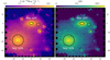 |
Fig. 1. Map of the median intensity (left panel) and S/N per spectral pixel of 1.1 Å (right panel) in the wavelength range 4400 Å–6650 Å. The coordinates are centred in NGC 1277 and are in arcseconds. The black continuous shapes denote the effective radii of the galaxies as measured in Sect. 3.2. The effective radius of NGC 1277 has been de-circularised assuming an axial ratio |

3. Galaxy resolved kinematics and MGE modelling
3.1. The resolved kinematics of NGC 1277 and NGC 1278
The kinematics of the field were obtained with pPXF3 (Cappellari & Emsellem 2004; Cappellari 2022). This code fits the spectra with a linear combination of spectral energy distribution templates convolved with a line-of-sight velocity distribution (LOSVD). The templates were drawn from the E-MILES single stellar population models4 (Vazdekis et al. 2015), which uses the MILES (Sánchez-Blázquez et al. 2006; Falcón-Barroso et al. 2011) and CaT (Cenarro et al. 2007) stellar templates. We used the models with a Kroupa initial mass function (Kroupa 2001) and BaSTI isochrones (Pietrinferni et al. 2004, 2006, 2009; Pietrinferni et al. 2013; Cordier et al. 2007), but the choice of a specific library plays little effect in the precise determination of the kinematics. To speed up the processing, we excluded the templates that, a priori, would not describe a massive ETG, that is those with low metallicity ([Z/H]< − 0.35) and young ages (< 1 Gyr). We have tested that producing the fits with the complete MILES model library would not introduce significant changes in the derived kinematics.
We only fitted the first two momenta of the LOSVD, that is the mean recession velocity and the velocity dispersion [v, σ]. The characterisation of higher-order momenta requires high-S/N data, which would go against our goal of covering as much of NGC 1277 as possible. In some lines of sight, two objects appear in projection, so their spectra should be fitted with two sets of templates with distinct kinematics. This is why each spectrum was at first fitted with single sets of templates with initial values [v = 5066 km s−1, σ = 250 km s−1] (corresponding to the redshift z = 0.016898 of NGC 1277; Falco et al. 1999), [v = 6066 km s−1, σ = 250 km s−1] (roughly the velocity of NGC 1278), [v = 4066 km s−1, σ = 50 km s−1] (the velocity of a small galaxy overlapping with part of the western side of NGC 1277; see Fig. 1), and [v = −34 km s−1, σ = 50 km s−1] (this is a velocity compatible with that of Galactic objects and it was chosen so to describe foreground stars), and with pairs of sets of templates combining the above initial values. The best fit was chosen based on the chi-squared values after penalising by a factor 1.1 fits with two sets of templates. The latter factor was manually selected after extensively testing which value was required not to use two templates in fitting spectra where a visual inspection clearly indicated the presence of a single object.
A necessary input of the Jeans modelling (Sect. 4) is a 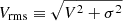 map, where V is the velocity corrected for the mean recession velocity of the galaxy vrec (V ≡ v − vrec). The recession velocity was obtained by assuming a symmetric rotation curve and by finding the average of the peak velocities of the receding and the approaching sides. We obtained a recession velocity of vrec = 5097 km s−1 for NGC 1277 and vrec = 6072 km s−1 for NGC 1278.
Figures 2 and 3 show the V, σ, and Vrms maps for NGC 1277 and NGC 1278, respectively. We are only plotting the fibres that were used for the Jeans modelling, that is those with high enough S/N (S/N > 7 per spectral pixel), low kinematic errors (ϵ(Vrms) < 65 km s−1; formal errors as derived by pPXF), and for which pPXF has converged to reasonable σ values (10 km s−1 < σ < 350 km s−1). Furthermore we only selected those with V within 400 km s−1 of vrec for NGC 1277 and within 60 km s−1 for NGC 1278. Those values are selected to be slightly larger than the amplitude of the rotation curve of the galaxies. Overall, the maps include 47 fibres for NGC 1277 and 183 for NGC 1278. The coverage of NGC 1277 is roughly elliptical in shape, with a semi-major axis of ∼18″ (6 kpc at the distance of NGC 1277, corresponding to five effective radii as measured in Sect. 3.2) and a semi-minor axis of ∼10″ (3.5 kpc). The coverage of NGC 1278 is roughly circular, with a radius of ∼30″ (10 kpc, or more than two effective radii).
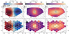 |
Fig. 2. Kinematic maps of NGC 1277. From left to right, V, σ, and Vrms maps of NGC 1277. The dashed line in the left panel indicates the kinematic major axis determined with kinemetry. The top row shows an interpolated version of the maps, whereas the lower one shows the individual fibre values. The grey contours denote isophotes separated by 0.5 mag arcsec−2 intervals obtained from an HST F625W image (top row) and from the integral field data integrated between 6150 Å and 6650 Å (lower row). The axes are in units of arcseconds. |
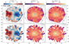 |
Fig. 3. Same as Fig. 2, but for NGC 1278. In order to highlight the kinematic structures, the colour scales differ from those in Fig. 2. In this case, the top-row isophotes are based on an HST F850LP image, which is the one used for the MGE modelling detailed in Sect. 3.2. Since for this galaxy V ≪ σ, the Vrms map is virtually identical to the σ map. |
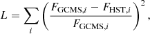
Because of the large angular size of the fibres compared to the size of NGC 1277, we had to devise a method to pinpoint the centre of the galaxy in the CGMS data. Initially, we aligned the GCMS data of both galaxies simultaneously with an HST Advanced Camera for Surveys (ACS; Ford et al. 1998) F850LP image (programme ID GO 14215; Trujillo et al. 2015). This was done by comparing the flux of the fibres selected for the Jeans modelling with that within circular apertures in the image with the same radius as the fibres. The HST image had previously been convolved with a Gaussian kernel with a sigma of one arcsecond so to match the seeing of the GCMS observations. The CGMS fluxes were calculated in the 6150 Å−6650 Å spectral range. We excluded bluer wavelengths in order to avoid a too large wavelength difference between the integral field and the HST data. Ideally, an HST image in a wavelength matching that of the CGMS data should have been used, but unfortunately the available ACS F625W image (programme ID GO 10546; Fabian 2005) does not fully cover NGC 1278. The determination of the exact alignment was obtained by minimising
 (1)
(1)
where FGCMS, i and FHST, i denote the flux for the ith bin in the CGMS fibre and the corresponding HST area, respectively. To deal with the differences in wavelength range between the two instruments and with possible flux calibration issues, we normalised FGCMS, i by setting ∑iFGCMS, i = ∑iFHST, i before applying Eq. (1). The minimisation was performed with the adaptive Metropolis et al. (1953) for Bayesian analysis code (adamet5; Cappellari et al. 2013a), which is an implementation of the algorithm by Haario et al. (2001).
The simultaneous registration of the two galaxies led to small systematics in the ratio (FGCMS, i − FHST, i)/FGCMS, i, indicating small inaccuracies in the coordinates of either the GCMS fibres or the HST pixels. As a consequence, we redid the registration by processing the two galaxies separately (using the F625W image for NGC 1277). Because a few fibres have a very different photometry from that of the matched HST apertures, we introduced a two sigma clipping to remove the outliers in (FGCMS, i − FHST, i)/FGCMS, i. The separate registration of the two galaxies resulted in centres that are  and
and  away from those obtained from a joint registration for NGC 1277 and NGC 1278, respectively. In Figs. 4 and 5, we show the relative differences of the GCMS fluxes and those derived from the matched apertures in the HST images. The residuals are generally at a level of ∼10% except at the very centre. We checked whether the latter discrepancies could be reduced by fine-tuning the seeing used for blurring the HST images, but failed to find a value leading to a significant improvement. This might either indicate that the Gaussian shape assumed for the point spread function (PSF) is too simplistic or a non-linearity in the behaviour of the GCMS.
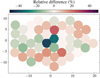 |
Fig. 4. Relative difference between the 6150 Å−6650 Å normalised flux of the GCMS fibres and the flux from matched apertures of an HST F625W image smoothed to mimic the seeing of the ground-based observations. |
As an alternative method for the GCMS data registration, we aligned four bright stars in the HST with their GCMS counterparts. The alignment differences between the two methods were of  only for NGC 1277. We decided to use the former registration method, but we have checked that using the latter alignment does not significantly change any of the results obtained from the JAM fit (Sects. 4.1 and 4.2). Actually, according to our tests, the fitted parameters of NGC 1277 are robust to changes in the centre of up to at least
  .
.
We determined the major axis of the galaxies photometrically by running the isophote routine from the Photutils package that uses the ellipse fitting method from Jedrzejewski (1987) over the HST F625W image (for NGC 1277) and the F850LP image (for NGC 1278). Point sources, overlapping galaxies were manually masked. The HST images reveal that both galaxies have a tiny circumnuclear dust ring smaller than 1″ in radius which is visually similar to some of those described in Lauer et al. (2005) and Comerón et al. (2010). The ring in NGC 1277 has already been reported by van den Bosch et al. (2012) and Emsellem (2013). The near side of those rings was masked too. The major axis position angles were extracted by averaging the orientation of the tilted rings over radial ranges where it is roughly flat (3″ ≤ R ≤ 10″ for NGC 1277 and 4″ ≤ R ≤ 20″ for NGC 1278). We find the position angles  and
and  for NGC 1277 and NGC 1278, respectively (Fig. 6). Our determination of the position angle for NGC 1277 is close to the value of
  reported in van den Bosch et al. (2012) and of
  from HyperLeda6 (Makarov et al. 2014).
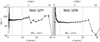 |
Fig. 6. Position angle as a function of distance along the major axis for the ellipse fit of the HST imaging of NGC 1277 (left) and NGC 1278 (right). The error bars correspond to the one-sigma uncertainties. The vertical dashed lines indicate the radial interval over which the kinematical axis was determined. Its estimated value is indicated by the number in the lower part of the panels and the horizontal dotted lines. |
We constructed velocity and velocity dispersion profiles using the information from the fibres that are crossed by the kinematic major axis. Figure 7 displays the rotation and the velocity dispersion curves for NGC 1277 in black (left panels). The profiles for NGC 1278 are also shown for reference. As a sanity check to assess the quality of our kinematic determination we also plot the previous long-slit measurements of NGC 1277 from Ferré-Mateu et al. (2017) in crimson (right panels). We find a smaller amplitude of the velocity curve than them. This is most likely because, while they explore a relatively narrow slit along the major axis of the galaxy ( in width Martín-Navarro et al. 2015), our resolution element is
  in radius, so it gathers light from regions with a significant tangential motion of the stars. Our σ profile agrees with that in Ferré-Mateu et al. (2017) except for the central peak which we are missing, most likely due to beam smearing. In principle, a small increase in the sigma of the disc is to be expected in our data because within each fibre we are sampling separated regions with different velocities. However, because these differences in velocity are of the order of at most ∼50 km s−1, they constitute an almost insignificant increase of up to ∼10 km s−1 over a typical velocity dispersion of 150 km s−1.
 |
Fig. 7. Velocity (top-row panels) and σ (lower-row panels) profiles for NGC 1277 (left-column panels) and NGC 1278 (right-column panels) as measured along the kinematic major axes. The black data points denote our measurements obtained from fibres whose centre is within the fibre radius ( |

The fact that in Fig. 7 both galaxies are shown with the same velocity and angular scales highlights the differences between the two. NGC 1277 is a compact fast rotator with a central σ cusp, while NGC 1278 is an extended barely rotating object with a much more uniform σ.
3.2. MGE models of HST images and mass maps
The density of the luminous tracers whose kinematics dominate the spectral range that we are studying (stars in our case) is a necessary input for JAM. Since we aim to obtain dark matter distributions, we also need to know the baryonic mass distributions to disentangle both kinds of matter.
To trace the luminosity of NGC 1277, we used an HST ACS F625W image with a Galactic extinction correction AF625W = 0.365 mag (Schlafly & Finkbeiner 2011) and also corrected for cosmological dimming. The filter was selected because it is within the spectral range from which we obtained the kinematics (4400 Å−6650 Å), so it is representative of the stellar population that dominates the stellar kinematics that we are tracing with our instrumental set-up. Unfortunately, NGC 1278 is only partially covered by the exposure. To model this galaxy, we instead used the ACS F850LP image with a correction AF850LP = 0.205 mag and corrected for cosmological dimming. This is not ideal, because this band falls outside the CGMS spectral range, and as a consequence does not exactly correspond to the stellar population of the luminous tracers. Because the F850LP image covers both galaxies, it is used as a proxy for the z band in the colour maps (see below).
The mass maps for both galaxies were constructed by combining the above-mentioned F850LP frame and an extinction- and cosmological dimming-corrected F475W image (AF475W = 0.538) from the same programme. Equating F475W to the g band and F850LP to the z band (Ryon 2022) and assuming a Chabrier (2003) IMF, Table A.1 from Roediger & Courteau (2015) provides the following relation for the g-band mass-to-light ratio:
 (2)
(2)
We did not account for the PSF mismatch because both bands have a Gaussian kernel with a very similar FWHM ( and
and  for F475W and F850LP, respectively as estimated with IRAF’s imexamine). We applied the mass-to-light ratio map to the F475W image to obtain the mass surface density map. We considered an absolute solar magnitude of M⊙g = 5.11 mag (Willmer 2018). Because of the strong evidence for a bottom-heavy IMF in red nuggets (Martín-Navarro et al. 2015; Ferré-Mateu et al. 2017), which is consistent with the tendency for the densest galaxies to have the heaviest IMF (Fig. 12 in Cappellari et al. 2013b), the mass density map was corrected from a Chabrier to a Salpeter (1955) IMF with the following recipe from Cimatti et al. (2008)
 (3)
(3)
This recipe does not account for the mass of stellar remnants.
Given that the outer regions of the galaxies contain pixels with no well-defined colours due to negative fluxes introduced by random fluctuations, we fixed the colours beyond a certain radius before producing the mass maps. For NGC 1277 the colours were fixed to those within an elliptical corona oriented along the galaxy major axis. The parameters of the corona were an ellipticity of 0.6 (from our isophote fits in Sect. 3.1), an outer semi-major axis of 9″, and a 0.9 times smaller inner semi-major axis. For NGC 1278 we used a circular corona with an outer radius of 15″ and an inner radius of 0.9 times that.
Both the surface brightness and the mass density distributions were parametrised using an MGE (Emsellem et al. 1994; Cappellari 2002). The fits were made with the MgeFit7 software by Cappellari (2002). This approach describes galaxies as a superposition of two-dimensional Gaussian components which, by knowing the inclination of the galaxy, can be deprojected into three-dimensional oblate axi-symmetric Gaussian components. We fixed the major axis of the MGE components to correspond to those of the kinematic axes measured in Sect. 3.1.
A detailed characterisation of the surface brightness and mass distributions requires knowledge about the PSFs. They were modelled using Tiny Tim (Krist 1995; Krist et al. 2011) and assuming that the targets sit at the centre of the chip. For the mass map, we adopted the PSF of the reddest filter used to build it, that is F850LP.
We modelled a region significantly larger than that covered by our good-quality integral field data, that is, an ellipse with  (from the kinematic major axis) and with semi-axes a = 640 pixels (32″) and b = 384 pixels (
 ) for NGC 1277 (the ellipticity was again set to 0.6), and a circle with a radius a = 900 pixels (45″) for NGC 1278. We used the same mask as for the isophote fit in Sect. 3.1. As done by Emsellem (2013), and in order to avoid roundish MGE components for NGC 1277, we imposed a maximum projected axial ratio of 0.7 for the components in this galaxy.
Tables 1 and 2 show the parameters of the MGE decompositions of the surface brightness and mass density maps of the two galaxies, respectively. The magnitude of the Sun in r (F625W) and z (F850LP) was assumed to be M⊙r = 4.65 mag and M⊙z = 4.50 mag, respectively (Willmer 2018). Figures 8 and 9 allow a direct visual comparison of the isophotes of the original HST images (in black) and those from the model (in red).
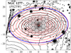 |
Fig. 8. Isophote plot derived from the HST F625W image of NGC 1277 with 0.5 mag arcsec−2 intervals (black contours). The corresponding MGE model isophotes are indicated in red. The blue ellipse denotes the extent of the region that was used to produce the MGE models (an ellipse with a semi-major axis of 32″, an ellipticity of 0.6, and a |

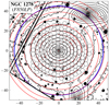 |
Fig. 9. Same as Fig. 8, but for NGC 1278 and the HST F850LP image. The fitted area (blue circle) is 45″ in radius. |
Parameters of the MGE decompositions of the surface brightness maps of NGC 1277 and NGC 1278.
Parameters of the MGE decompositions of the surface mass density maps of NGC 1277 and NGC 1278.
As a sanity check, we compared our MGE major- and minor-axis surface brightness profiles for NGC 1277 to those in Emsellem (2013). We corrected the latter for Galactic extinction to be directly comparable with ours. The profiles were computed following Eq. (1) in Cappellari (2002)
![Mathematical equation: $$ \begin{aligned} I(x,{ y})=\sum _jI_{0j}\,\mathrm{exp}\left[-\frac{1}{2\sigma _{{\star }j}^2}\left(x^2+\frac{{ y}^2}{q^{\prime }_{{\star } j}}\right)\right], \end{aligned} $$](/articles/aa/full_html/2023/07/aa46291-23/aa46291-23-eq30.gif) (4)
(4)
where the sum is made over all the Gaussian components j, x and y are coordinates in the plane of the sky (in the directions of the major and the minor axis of the galaxy, respectively), and I0j, σ⋆j, and  are the central surface brightness, the dispersion (size), and the projected axial ratio of the MGE components. The results are shown in Fig. 10.
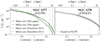 |
Fig. 10. Major- (continuous line and coordinate x) and minor-axis (dashed line and coordinate y) surface brightness profiles of NGC 1277 (left panel; in F625W) and NGC 1278 (right panel; in F850LP). Black lines come from our MGE fit and green ones come from Emsellem (2013) after a correction for extinction. The vertical grey lines indicate the maximum extent of the fitting area along the major (continuous) and the minor axis (dashed). For NGC 1278 the minor and major axis surface brightness profiles are nearly undistinguishable. The grey curves in the right panel correspond to the F625W surface brightness profiles calculated under the assumption that r − z = 0.74 (see text). |
Overall, the agreement between our parametrisation of the surface brightness map of NGC 1277 and that from Emsellem (2013) is rather good. The apparently large difference within the central  only affects the central pixel. The other small discrepancies within the central 1″ can be attributed to differences in the handling of the small nuclear dust ring. Some large differences are seen at the edges of the fitting range, where the surface brightness profiles computed from our fit can be, at very specific radii, a factor of two or more above that obtained from Emsellem (2013). This occurs at a surface brightness of ∼25 mag arcsec−2 and might be a consequence of small differences in sky subtraction, masking strategies, or the extent of the fitted area.
The total F625W luminosity of our NGC 1277 model can be calculated as (Cappellari et al. 2013a, Eq. (10))
 (5)
(5)
where Lj is the total luminosity of each of the individual Gaussian components, resulting in L = 2.6 × 10¹⁰ L⊙r. The luminosity estimated from the Emsellem (2013) parametrisation (after the extinction correction) is L = 2.6 × 10¹⁰ L⊙r too when using the same cosmology as us.
Our models show that NGC 1278, as expected, is more extended than NGC 1277. The central surface brightness of NGC 1278 is smaller than in NGC 1277, again indicating that the latter is a much more centrally concentrated object. The total F850LP luminosity of our NGC 1278 model is L = 8.7 × 10¹⁰ L⊙z. Given r − z = 0.74 (r − z = 0.90, when not accounting for differential extinction) as measured from a circular aperture 15″ in radius centred in NGC 1278 in SDSS DR16 images (Ahumada et al. 2020), this corresponds to L ≈ 5.8 × 10¹⁰ L⊙r, which is roughly two times the luminosity of NGC 1277 at the same band.
The circularised luminosity integrated within a cylinder of radius R of an MGE model can be written as (Cappellari et al. 2013a, Eq. (11))
![Mathematical equation: $$ \begin{aligned} L(R)=\sum _{j}L_j\left[1-\mathrm{exp}\,\left(-\frac{R^2}{2\sigma _{{\star }j}^2q_{{\star }j}^{\prime }}\right)\right]. \end{aligned} $$](/articles/aa/full_html/2023/07/aa46291-23/aa46291-23-eq34.gif) (6)
(6)
This expression can be used to find the effective radius of the galaxies by setting L(Re) = L/2. For NGC 1277 we obtain  (corresponding to 1.2 kpc) and for NGC 1278 we find
  (4.2 kpc). These values highlight again the extreme compactness of NGC 1277 when compared to a regular massive ETG. Our determination of the effective radius of NGC 1277 is comparable with the values of Re = 1.6 kpc obtained by van den Bosch et al. (2012, assumed distance d = 73 Mpc), Re = (1.2 ± 0.1) kpc by Ferré-Mateu et al. (2017), and Re = (1.3 ± 0.1) kpc by Yıldırım et al. (2017, d = 71 Mpc). Because the two galaxies differ in luminosity by a factor of roughly two, it might be convenient to describe their compactness in terms of their effective radius relative to that of a given isophote. We chose R23, the circularised radius of the 23 mag arcsec−2 extinction- and cosmological dimming-corrected F625W isophote. The circularised surface brightness profile was computed by setting
  and
and  in Eq. (4) as suggested in Cappellari et al. (2009). We obtained R23/Re = 5.1 and R23/Re = 2.9 for NGC 1277 and NGC 1278, respectively.
Using the data in Table 2 we derived the surface density profiles (Fig. 11), which we found to follow rather closely the surface brightness profiles except for the inner arcsecond, where the colours differ from the rest of the galaxy due to the presence of dust rings. These profiles have to be taken with some care, since they are made under the assumption of a Salpeter IMF. Different IMFs might result in significant Υ⋆ changes (see Sects. 4 and 5.1 for a dynamical determination of Υ⋆). Under this IMF assumption we use an expression analogous to Eq. (5),
 (7)
(7)
 |
Fig. 11. Major- (continuous line and coordinate x) and minor-axis (dashed line and coordinate y) stellar surface density profiles of NGC 1277 (left panel) and NGC 1278 (right panel). The vertical grey lines are as in Fig. 10. The surface density estimates were calculated by deriving pixel-to-pixel mass-to-light ratios from colours following the prescriptions in Roediger & Courteau (2015), and assuming a Salpeter IMF. |
to find a total stellar mass of M⋆ = 1.3 × 10¹¹ M⊙ for NGC 1277 (compatible with the value of M⋆ = (1.3 ± 0.2)×1011 M⊙ in Yıldırım et al. 2017, for a distance d = 71 Mpc) and of M⋆ = 2.9 × 10¹¹ M⊙ for NGC 1278.
4. JAM dynamical modelling
We used the Jeans Anisotropic Modelling (JAM8) code to produce dynamical models of the galaxies. A basic assumption of JAM is that the galaxies are axisymmetric. Given MGE models of the luminous tracer and mass distributions, a galaxy inclination (i), and an anisotropy parameter (βz or βr) that can be different for each MGE component, JAM computes the projected first and second moments of the velocity distribution of the dynamical tracers (stars in our case). JAM solves the Jeans equations to describe the motions of star in a state of hydrodynamical equilibrium (Jeans 1922) by assuming either a cylindrically (Cappellari 2008) or a spherically aligned velocity ellipsoid (Cappellari 2020). The definition of the anisotropy parameter varies depending on the chosen alignment. In the cylindrically aligned case, with coordinates (R, z, θ), the anisotropy parameter is defined as  , whereas for the spherically aligned case with coordinates (r, θ, ϕ),
  (Vz, VR, Vθ, and Vr stand for the velocities along the z, R, θ, and r coordinates, respectively). We fitted the JAM models to the Vrms values obtained from the GCMS and NIFS observations using adamet. Before running the fits, we rotated the Vrms maps so that the major axis of the galaxy determined in Sect. 3.1 lied horizontally.
Tests of JAM using high-resolution N-body simulations (Lablanche et al. 2012) and lower-resolution cosmological hydrodynamical simulations (Li et al. 2016) have confirmed its good accuracy when using high-S/N data, and negligible bias in reproducing the total mass profiles. More recently, JAM was compared in detail against the Schwarzschild (1979) method using samples of both observed galaxies, with circular velocities from interferometric observations of the CO gas, and numerical simulations respectively. These studies consistently found that the JAM method produces even more accurate (smaller scatter versus the true values) density profiles (Fig. 8 in Leung et al. 2018) and enclosed masses (Fig. 4 in Jin et al. 2019) than the more general Schwarzschild models. This may be due to the JAM assumption acting as an empirically motivated prior and reducing the degeneracies of the dynamical inversion. These extensive tests justify our choice of JAM for this study.
In general, our density models introduced into adamet include the dark matter halo, the stellar component, and a central mass to account for the supermassive black hole. The latter is introduced as a minute MGE component with a Gaussian sigma of  .
.
We assumed spherical dark matter haloes described by a Navarro-Frenk-White profile (NFW profile Navarro et al. 1996, 1997)
 (8)
(8)
where r is the three-dimensional radius, rs is the break radius, and ρs is a normalisation density. In order to reduce the number of free parameters, we set rs = 100 kpc, which is a reasonable estimate for massive elliptical galaxies calculated from the stellar-to-halo mass relation from Girelli et al. (2020) and the halo mass-concentration relations from Klypin et al. (2011) and Child et al. (2018, see Sect. 5.2 for further details). As discussed in Cappellari et al. (2013a), the choice of a break radius is irrelevant because simulations systematically predict them to be found well outside the outermost regions sampled by the dynamical tracers. To include the dark matter halo in our JAM models, we fitted the analytic form of the halo with the mge_fit_1d routine in the MgeFit package, which produces an accurate MGE approximation. The dark matter halo Gaussian components were characterised by their mass MDM j and dispersion σDM j.
The three-dimensional stellar mass distribution fed into JAM was that from the MGE stellar mass density models (Sect. 3.2). The intrinsic axial ratio of the Gaussian components was obtained by assuming an inclination angle i (Cappellari 2008, Eq. (14))
 (9)
(9)
Once the intrinsic axial ratios of the components were computed, the volume density of stars was described as
![Mathematical equation: $$ \begin{aligned} \rho _\star (R,z)=\alpha \sum _j\frac{M_{\star j}}{\left(\sqrt{2\pi }\sigma _{{\star }j}\right)^3q_{\star j}}\,\mathrm{exp}\,\left[-\frac{1}{2\sigma _{{\star }j}^2}\left(R^2+\frac{z^2}{q_{{\star }j}^2}\right)\right], \end{aligned} $$](/articles/aa/full_html/2023/07/aa46291-23/aa46291-23-eq45.gif) (10)
(10)
where R is the projection of the radius in the mid-plane of the galaxy, and where the formula from Cappellari (2008) is scaled with the so-called mismatch parameter (Cappellari et al. 2012), which is defined as
 (11)
(11)
The mismatch parameter describes the stellar mass-to-light ratio with respect to that expected from a Salpeter IMF.
In practice, we fitted up to five parameters by feeding JAM models into adamet. These parameters are:
-
(1)
The intrinsic axial ratio of the flattest MGE component of the stellar model, q⋆ min. It is related to the projected axial ratio
 and the inclination i through Eq. (9). Fitting this parameter is equivalent to fit the inclination i.
 -
(2)
The shape of the velocity ellipsoid, parametrised by either βz or βr.
-
(3)
The mismatch parameter, that accounts for deviations from the Salpeter IMF that was assumed while constructing the stellar mass maps (Sect. 3.2). Finding this parameter is equivalent to a dynamical determination of the stellar mass-to-light ratio.
-
(4)
The black hole mass, MBH.
-
(5)
The dark matter halo density normalisation. We introduced it as fDM(6 kpc), the fraction of matter that is dark within the inner 6 kpc of the galaxy. The mass within 6 kpc was calculated as M(6 kpc) = M⋆(6 kpc)+MDM(6 kpc)+MBH. The seemingly arbitrary 6 kpc radius corresponds to the radial coverage of the GCMS data of NGC 1277. When computing fDM(6 kpc) we have counted the central black hole mass as baryonic mass.
We adopted constant priors on all parameters during the adamet Bayesian modelling. For most of the parameters, we refined the bounds of the fitting range after running the fit several times and examining the posterior probability distributions. In other cases, the boundaries come from physical limitations. For example, MBH and fDM(6 kpc) cannot be smaller than zero. Also, the intrinsic axial ratio of the flattest MGE component cannot be larger than the projected one, setting an upper boundary  . Finally, to avoid unphysically thin components, we assume a minimum possible axial ratio for the flattest component at q⋆ min = 0.05.
In order to calculate the mass of spherical dark matter halo MGEs within a specific radius we used the following expression from Cappellari (2008, Eq. (49))
![Mathematical equation: $$ \begin{aligned} M_{\rm DM}(r)=\sum _jM_{\mathrm{DM}\,j}\left[\mathrm{erf}\,\left(\frac{r}{\sqrt{2}\sigma _{\mathrm{DM}\,j}}\right)-\frac{\sqrt{\frac{2}{\pi }}r}{\sigma _{\mathrm{DM}\,j}}\mathrm{exp}\,\left(-\frac{r^2}{2\sigma _{\mathrm{DM}\,j}^2}\right)\right], \end{aligned} $$](/articles/aa/full_html/2023/07/aa46291-23/aa46291-23-eq49.gif) (12)
(12)
where erf stands for the error function. For the flattened stellar MGE components, the mass contained within a radius r is given by the following expression adapted from Cappellari et al. (2013a, Eq. (15))
![Mathematical equation: $$ \begin{aligned} M_\star (r)=\alpha \sum _jM_{\star j}\left[\mathrm{erf}\,\left(h_{\star j}\right)-2h_{\star j}\mathrm{exp}\,\left(-h_{\star j}^2\right)/\sqrt{\pi }\right], \end{aligned} $$](/articles/aa/full_html/2023/07/aa46291-23/aa46291-23-eq50.gif) (13)
(13)
where we accounted for the mismatch parameter, and where
 (14)
(14)
The instrumental pixel size and the seeing are accounted for by JAM. Since the pixels considered by JAM are square, for GCMS we assumed a pixel size of  , equivalent in surface to our
  in diameter fibres. We also assumed a PSF sigma of one arcsecond. For the NIFS data the situation is more complicated, because the data points correspond to the centre of Voronoi bins with variable size. We set the pixel size to the native value for NIFS,
  , because the data for the central region of NGC 1277 (the most sensitive to the black hole dynamics) has enough signal to remain unbinned. We used the same NIFS PSF parametrisation as Krajnović et al. (2018, Appendix A), that is an inner component with a Gaussian sigma
  and weight 0.65 and an outer component with sigma
  and a weight 0.35.
4.1. Dynamical modelling of NGC 1277
For NGC 1277 we have both GCMS and NIFS data. A particularity of the NIFS dataset is that the spaxel with the largest σ does not correspond to the coordinate centre as provided by Walsh et al. (2016). This small offset of  was corrected before running the fits.
We tested three fitting approaches to check the internal consistency and gauge the uncertainties:
A. Successively fit the NIFS and the GCMS data: We first fitted the NIFS data (A1; Fig. 12). Since the field of view of the instrument only covers the inner 0.5 kpc of NGC 1277, we assumed the dynamical effect of dark matter to be negligible and fixed fDM(6 kpc) = 0. Indeed, the dark matter fraction within 0.5 kpc expected for a dark matter halo typical of a galaxy with the mass of NGC 1277 (see Sect. 5.2) is ∼0.5%. Then, we fitted the GCMS data with the black hole mass MBH fixed to the value obtained in A1 (A2; Fig. 13). The rationale for this is that the black hole sphere of influence (Peebles 1972) is small compared to the field of view covered by the GCMS data (∼130 pc or  for a MBH = 5 × 10⁹ M⊙ and for a central velocity dispersion σ = 400 km s−1) and we should not expect the latter to help constraining the black hole mass. When fitting for black hole masses with JAM, it is always recommended to restrict the field of view to the smallest region required to break the M/L-black hole degeneracy (e.g. Thater et al. 2022) not to risk biasing the black hole mass due to gradients in the velocity ellipsoid and the mismatch parameter, or due the choice of a parametrisation for the dark matter halo. In other words, a good global fit might be reached at the expense of a poor fit of the central region, resulting in a bad determination of the black hole mass. This approach is very different from the one usually employed with Schwarzschild models, which need large radii kinematics to constrain the orbital distribution and reduce degeneracies in the black hole mass.
 |
Fig. 12. Dynamical modelling of the NIFS Vrms map of NGC 1277 assuming a cylindrically aligned velocity ellipsoid (fit cA1). The corner plot shows the probability distribution of the fitted parameters marginalised over either two parameters for the contour plots, and over one for the histograms. In the contour plots blue regions correspond to the three-sigma confidence level and white regions denote maximum likelihood. The top-right corner shows the Vrms map and the fit, with grey isophotes indicating F625W contours separated by 0.5 mag arcsec−2 and the black crosses indicating the centre of the bins. The indentations in the isophotes are a clear sign of the presence of the dust ring, whose near side was masked while producing the MGE models. The fitted parameters were q⋆ min, βz, α, and MBH, whereas the dark matter fraction fDM(6 kpc) was fixed to zero. |
B. Simultaneous fit of the NIFS and the GCMS data: Both sets of data were fitted simultaneously (plot not shown). We multiplied the uncertainties of Vrms in the NIFS dataset by a factor 2.5 so both datasets have a roughly equal weight in the chi-squared value (the same procedure was followed in Cappellari et al. 2015, to merge data from SLUGGS and ATLAS3D).
C. Fitting the GCMS data alone: For this fit, we excluded the NIFS data (plot not shown). As detailed in the description of approach A, this procedure is not recommended because we run into the risk of biasing the black hole mass estimate. However, because we do not have NIFS data for NGC 1278, producing this fit allows for a direct comparison between the two galaxies.
We denote fits made assuming a cylindrically aligned velocity ellipsoid with a ‘c’ prefix, and those with a spherically oriented one with an ‘s’. As discussed in Cappellari (2020), no single alignment holds for a full galaxy. A cylindrically oriented ellipsoid is only found in the case of a plane-parallel potential, whereas a spherically oriented one is found for a strictly spherical one. Nevertheless, a cylindrically oriented ellipsoid is a rather good approximation for a disc, especially close to the mid-plane (Cappellari et al. 2007; Cappellari 2008). Since the Schwarzschild (1979) dynamical modelling by Yıldırım et al. (2015) does not show signs of a galaxy-wide pressure-supported component, we assumed a cylindrical alignment for our fiducial fit of NGC 1277 (cA).
The fitted parameters for all the approaches are listed in Table 3. For parameters whose maximum likelihood values are not close to the boundary of the fitting interval, we present them as value ± sigma/2, where sigma has been calculated as the interval between the 15.86 and 84.14 percentiles. In some cases, in particular for fDM(6 kpc) and q⋆min, the probability distribution may peak close to the boundary of the fitting interval imposed by physics. We detected those cases are those where |value−boundary| < sigma/2. In such cases, we determined one-sigma upper (lower) limits based on the 68.28 (31.72) percentile.
JAM model fit parameters for NGC 1277.
We first comment on the fiducial fit, cA. When fitting the NIFS data only we find a black hole mass MBH = (4.88 ± 0.11)×109 M⊙ (Fig. 12), which is very similar to MBH = (4.54 ± 0.11)×109 M⊙ obtained by Krajnović et al. (2018) with the same data. The fitted values for q⋆ min and β are the same within the uncertainties. The subsequent GCMS data fit with a fixed MBH (Fig. 13) yields a negligible dark matter fraction with fDM(6 kpc) < 0.018. We find that the mismatch parameter is very similar for the NIFS and the GCMS fits (only a 5% difference; α = 1.342 ± 0.014 versus α = 1.276 ± 0.013). This is relevant, since a large difference between the two would require considering an α varying with radius. The determination of the mismatch parameter in the cA2 fit allows us to re-evaluate the stellar mass of NGC 1277 to M⋆ ≈ 1.8 × 10¹¹ M⊙.
 |
Fig. 13. As Fig. 12, but this time the fitted Vrms map is that of the GCMS data, fDM(6 kpc) (fDM(1.5 Re)) is a free parameter and the central black hole mass is fixed to MBH = 4.70 × 10⁹ M⊙ (fit cA2). As in Fig. 2, the Vrms maps are displayed in their interpolated (left) and individual-fibre (right) forms. They surface brightness contours correspond to HST data for the interpolated maps and to photometry derived from the CGMS data for the non-interpolated ones. |
In Figs. 14 and 15 we compare the major- and minor-axis Vrms profiles of the NIFS and GCMS data to those derived from the cA1 and cA2 fits, respectively. The agreement between the data and the fits is generally good, especially for the GCMS data (cA2), where the fitted Vrms passes close to most of the observed data points when accounting for three-sigma error bars. The central small Vrms peak is also well captured by the fit.
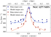 |
Fig. 14. Major- (blue) and minor-axis (red) Vrms profiles for the NIFS data of NGC 1277 (symbols) and the cA1 fit (continuous line). The error bars represent one-sigma Vrms formal uncertainties as obtained by pPXF (see Sect. 3.1). We selected the bins whose centres are within a cone with an aperture of 30° centred in the major (minor) axis. |
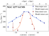 |
Fig. 15. Same as Fig. 14, but this time for the GCMS data, the cA2 fit, and for fibres whose centre is within a fibre radius ( |

Both fitting approaches cB and cC yield very similar values for several of the parameters, with negligible dark matter fractions within 6 kpc, a mismatch parameter α ≈ 1.3, and a black hole mass in the range 2.6 × 10⁹ M⊙ ≲ MBH ≲ 4.9 × 10⁹ M⊙. It is noteworthy that the high angular resolution NIFS data do not seem to be required to obtain a reasonable order of magnitude estimate of the black hole mass. This is probably due to the fact that we are introducing high angular resolution information through the MGE models of the luminosity and the surface brightness distributions (see Appendix A) and highlights the importance of high angular resolution information to properly constrain the mass of the central black hole. A further reason for the black hole mass agreement is that the mismatch parameter does not vary much with radius, as indicated by the small difference in the α values fitted in cA1 and cA2.
The intrinsic flattening of the flattest component q⋆ min shows significant differences between fitting approaches. This parameter is found to be in the range between q⋆ min = 0.050 and q⋆ min = 0.4, which corresponds to an inclination between i = 67° and i = 90°. The intermediate q⋆ min values given by fit cA2 corresponds to i ≈ 76°, which is very close to the value deduced from the shape of the circumnuclear dust ring (i = 75°; van den Bosch et al. 2012). The value of q⋆ min < 0.06 obtained from fitting the NIFS data only is considerably off the other values, probably because the NIFS FOV covers a region where the dominant MGE components are nearly round (Table 2), hence offering little constraining power on the flatness of the galaxy.
The parameter βz is significantly smaller when fitting the NIFS data alone than when fitting GCMS data. This suggests a radial variation of the shape of the velocity ellipsoid. To explore this effect, we repeated all the fits where GCMS data are used, but this time we considered two βz parameters. The first one corresponded to stellar MGE components with a sigma smaller than the effective radius Re, whereas the second one (βz, out) described the more extended components. The fits with two βz values are denoted with the suffix ‘βz’. The results of the fits (Table 3) indicate that allowing for radial variations in βz does not have a significant effect in either α, MBH, or fDM(6 kpc).
Following Cappellari (2020), we also fitted the data assuming a spherically aligned velocity ellipsoid (with an anisotropy parameter βr) in order to have a better grasp of the uncertainties. The results remain broadly the same as with the cylindrically aligned models (Table 3) and a negligible dark matter fraction is also recovered.
We have also made experiments with dark matter profiles other than NFW, such as the generalised NFW profile or the Einasto profile (Einasto 1965). In all cases, the resulting dark matter fraction fDM(6 kpc) has been found to be compatible with zero. We also checked that uncertainties of the order of  in the determination of the centre of NGC 1277 within the field of view of the GCMS (see Sect. 3.1) do not affect our results.
To sum up, the results of all our fitting approaches broadly coincide with those of the fiducial fit cA (with a cylindrically aligned velocity ellipsoid and a single βz). This fit yields a mismatch parameter α = 1.342 ± 0.014 (giving a probably too optimistically well-constrained stellar mass of M⋆ ≈ (1.790 ± 0.019)×1011 M⊙) and a black hole mass MBH = (4.88 ± 0.11)×109 M⊙. We also find a negligible dark matter fraction within 6 kpc (5 Re), fDM(6 kpc) < 0.018. We stress that, irrespectively of the fitting approach, we find that dark matter has a negligible dynamical effect within the inner 6 kpc of NGC 1277 under the assumption of a mismatch parameter that is constant with radius.
4.2. Dynamical modelling of NGC 1278
In order to fit the NGC 1278 kinematics we need to rely on the GCMS data only. This means that, contrary to the case of NGC 1277, we lack high angular resolution data able to provide tight constraints on the black hole mass. For these fits we followed two approaches:
A. Fit where the central black hole mass is fixed by scaling relations: We use the MBH − M⋆ scaling relation in the Eq. (15) from Sahu et al. (2019) relating the black hole mass to the total stellar mass of elliptical galaxies (the plot for fit A is not shown). By introducing the total stellar mass M⋆ = 2.9 × 10¹¹ M⊙ (Sect. 3.2) we obtained MBH = 1.5 × 10⁹ M⊙. However, because the residual mean square of the relation is 0.48 dex, MBH is expected to be in the rather large range between MBH ≈ 5 × 10⁸ M⊙ and MBH ≈ 5 × 10⁹ M⊙. Alternatively, we could have used the MBH − σ relation. Assuming the expression in Eq. (7) from Kormendy & Ho (2013) and a central velocity dispersion σ = 285 km s−1 we obtained a virtually identical black hole mass of (MBH = 1.4 × 10⁹ M⊙ with a 0.29 dex scatter in the relation).
B. Fit with no constraints: We left all the parameters free, including the black hole mass MBH. We chose it to be our fiducial fit (Fig. 16) because the large scatter in the black hole scaling relations (see item A) could introduce a bias when fixing the black hole mass.
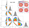 |
Fig. 16. Same as Fig. 12, but this time for the GCMS Vrms map of NGC 1278 assuming a spherically aligned velocity ellipsoid (fit sB). The isophotes in the left-column maps come from an F850LP image. This is our fiducial fit for NGC 1278, where the fitted parameters are q⋆ min, βr, α, and MBH, and fDM(6 kpc) (fDM(1.5 Re)). |
The baryon distribution in NGC 1278 is found to be nearly circular in projection (Table 2), which might be indicative of a far from flattened baryonic matter distribution. We tested this hypothesis by calculating the projected angular momentum within an effective radius to check whether NGC 1278 is a slow rotator, as follows. First, we estimated the projected angular momentum within Re (Emsellem et al. 2007, Eq. (6))
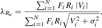 (15)
(15)
where the sums are made over the fibres within Re, Ri are the distances of the fibres to the centre of NGC 1278, and Fi are the fluxes at those distances based on the MGE model calculated using the circularised version of Eq. (4) (see Sect. 3.2). We found λRe = 0.093. Then, we measured the ellipticity of the MGE model using the routine mge_half_light_isophote included in JAM and obtained εe = 0.18. Finally, we applied the test proposed in Eq. (19) in Cappellari (2016), who suggested that galaxies fulfilling
 (16)
(16)
as it is the case for NGC 1278, are slow rotators. Since this test proves that NGC 1278 is not likely to be a very flattened object, we chose a spherically aligned velocity ellipsoid for our fiducial fit. We present the results in Table 4. As for NGC 1277, the fits are labelled with prefixes ‘c’ and ‘s’ so to denote the velocity alignments and a suffix ‘βz’ or ‘βr’, respectively, if they were produced assuming two different values for the shape of the velocity ellipsoid. Here we assumed that βr, out and βz, out affect the shape of the MGE components with σ⋆ larger than the effective radius,  .
.
JAM model fit parameters for NGC 1278.
Our fiducial fit sB (Fig. 16) yields a significant fraction of dark matter within 6 kpc, fDM(6 kpc) = 0.14 ± 0.04. This fraction does not change if we keep the black hole mass fixed (fit sA). The fiducial fit yields a mismatch parameter α = 1.16 ± 0.06, which implies that the stellar mass-to-light ratio is slightly larger than that expected from a Salpeter IMF. In principle, changes in α modify the MBH obtained in the MBH − M⋆ scaling relation that is introduced as a constant in sA, but since α ≈ 1, the shift in MBH would be very small. The value of MBH < 0.7 × 10⁹ M⊙ obtained in the fiducial fit is compatible with what is expected from the scaling relations.
All the fits yield a q⋆ min value peaking at or close to the boundary of the fitting range (q⋆ min = 0.75). Since NGC 1278 is likely to be near-spherical, this is a poorly defined parameter and not much importance should be attached to this coincidence.
Contrarily to NGC 1277, where fDM(6 kpc) was consistently found to be negligible irrespective of the kind of fit, the fraction of dark matter within 6 kpc in NGC 1278 is found to vary depending on whether a cylindrically or a spherically aligned velocity ellipsoid is assumed. The former orientation yields dark matter fractions fDM(6 kpc) = 0.02 − 0.04 and the latter have fDM(6 kpc) = 0.10 − 0.15. Fits with low fDM(6 kpc) compensate the lack of dark matter by increasing the baryonic mass through an increase in α from α ≈ 1.1 − 1.2 (slightly larger than that expected for a Salpeter IMF) to up to α ≈ 1.3 (indicating a bottom-heavy IMF comparable to that obtained for NGC 1277). For our fiducial fit, a zero dark matter fraction is disfavoured at a more than four-sigma level, but a strong covariance is seen between α and fDM(6 kpc) (Fig. 16). Hence, an independent determination of α would be desirable in order to confirm the presence of a significant dark matter fraction. Such evidence was obtained from line index indicators, showing a much bottom-lighter IMF in NGC 1278 than in NGC 1277 (Ferré-Mateu et al., in prep.).
Figure 17 shows the radial Vrms profile. The agreement between the observation and the fit in the central region (R ≲ 15″) is remarkable. At larger radii, the error bars in Vrms for the individual fibres becomes as large as a few tens of km s−1, which causes a large scatter. Yet, the fit passes roughly through the middle of the data cloud. The reason why such data points with large error bars are not abundantly found for NGC 1277 is the abruptness of the surface brightness profile, which causes the radial range of fibres with barely acceptable kinematic fits to be very narrow.
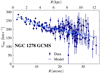 |
Fig. 17. Same as Fig. 14 but for NGC 1278 with GCMS data, and the SB fit. Because the galaxy is nearly spherical, we included data from all the fibres and sorted them according to their distance to the centre. |
As for NGC 1277, we checked whether registration errors of the GCMS data would have an impact on the results. We found that the uncertainties in α and fDM(6 kpc) introduced by a centring error of up to 1″ are comparable to the formal one-sigma error bars of the fit.
In summary, for NGC 1278 we find a dark matter fraction fDM(6 kpc) = 0.14 ± 0.04 and a black hole mass MBH < 0.7 × 10⁹ M⊙. The excess parameter is α = 1.16 ± 0.06 (slightly larger than for a Salpeter IMF), which yields a total stellar mass M⋆ = (3.4 ± 0.2)×1011 M⊙.
5. Discussion
5.1. The mass-to-light ratio and the IMF of the stellar component of NGC 1277 and NGC 1278
Our determination of the stellar mass of NGC 1277 and NGC 1278 makes it possible to provide constraints on the IMF. Our fiducial fit of NGC 1277 yields a stellar mass-to-light ratio in F625W (similar to the r band) Υ⋆r = 7.0 M⊙/L⊙r. After converting the F850LP surface brightnesses to F625W through r − z = 0.74 (measured from SDSS images, Sect. 3.2), we find Υ⋆r = 5.8 M⊙/L⊙r for NGC 1278.
If we know Υ⋆, the age of the stellar population, and its metallicity, we can obtain information about the shape of the IMF from photometric predictions based on spectral energy distributions. Here, we used those based on E-MILES (Vazdekis et al. 2012)9 computed using BaSTI isochrones. These predictions are made assuming an IMF lower cutoff at 0.1 M⊙ and an upper cutoff at 100 M⊙. The Υ⋆ inferences account for the stellar remnants (contrarily to the mass maps derived in Sect 3.2, with respect to which the mismatch parameter α from our fits was calculated). Based on Martín-Navarro et al. (2015) and Ferré-Mateu et al. (in prep.) we assume an age of 13.0 Gyr and a metallicity of [Z/H] = 0.26 for NGC 1277.
Under the assumption of a bimodal IMF with a turning point at 0.4 M⊙ defined as in Vazdekis et al. (1996), and where −Γb corresponds to the exponent of the power law in the high-end of the IMF, we obtain Γb = 2.46. This value is very similar with that found by Martín-Navarro et al. (2015) and Ferré-Mateu et al. (2017), where the index varied between Γb ≈ 3.05 ± 0.20 at the very centre of NGC 1277 and Γb ≈ 2.55 ± 0.40 at a radius of about 1.4 Re. The fact that both line-strength indices and dynamical modelling yield similar results makes the inference of a bottom-heavy IMF for NGC 1277 very robust.
In Fig. 18 we plot the stellar mass-to-light ratio at F625W as a function of the radius for NGC 1277 and NGC 1278. Here we define Υ⋆r as the ratio of the circularised surface density and the surface brightness MGE models corrected (multiplied) by the mismatch parameter. The right axis indicates the corresponding absolute value of the outer exponent of a bimodal IMF, Γb, obtained from the E-MILES photometric predictions for a stellar population with age 13.0 Gyr, metallicity [Z/H] = 0.26 (this is roughly valid for NGC 1277 only, because NGC 1278 is slightly younger and less metallic; Ferré-Mateu et al., in prep.). If the mismatch parameter, α, were constant with radius as assumed in the JAM fits, the wiggles in Υ⋆ would imply a genuine variation of the mass-to-light ratio. However, the observed changes in Γb, are a combination of real variations driven by small radial changes in α, and apparent variations due to small radial trends of the stellar population age and abundances. Nevertheless, it is reassuring to see that the estimated Γb index for NGC 1277 falls within the range of values obtained in Martín-Navarro et al. (2015) and Ferré-Mateu et al. (2017). In NGC 1278, Υ⋆ is systematically lower than in NGC 1277 at all radii. This is in line with the finding that relic galaxies have a bottom-heavier IMF than regular ETGs with similar properties (Martín-Navarro et al. 2023).
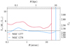 |
Fig. 18. Circularised mass-to-light ratio Υ⋆r as a function of the radius for NGC 1277 and NGC 1278, in blue and red respectively. The vertical lines indicate the limit of the GCMS kinematic data, The right axis shows the correspondence with the absolute value of the outer exponent of a bimodal IMF, Γb, for a stellar population with an age of 13.0 Gyr and a metallicity [Z/H] = 0.26. The horizontal black dashed lines denote the range of Γb values found by Martín-Navarro et al. (2015) for NGC 1277, with the upper line (Γb = 3.25) corresponding to their upper limit for the inner parts of the galaxy and the lower line (Γb = 2.15) corresponding to their lower limit at a radius R = 1.4 Re. The surface brightness of NGC 1278 has been converted to F625W as in Sect. 3.2. The correspondence between Υ⋆r and Γb is only roughly valid for NGC 1277 because NGC 1278 is slightly younger and less metallic (Ferré-Mateu et al., in prep.). |
5.2. The dark matter haloes of NGC 1277 and NGC 1278
In this subsection we compare the fitted dark matter haloes to the expectations from models and simulations. To do so, two pieces of information are required:
-
(1)
A stellar-to-halo mass relation (SHMR) providing a dark halo mass as a function of the measured stellar mass.
-
(2)
A parametrisation of the three-dimensional radial profile of the dark matter halo as a function of its mass.
We adopted the SHMR from Girelli et al. (2020), who used abundance matching to relate the observed stellar mass of galaxies in the COSMOS field to dark matter halo masses extracted from DUSTGRAIN-pathfinder ΛCDM simulation (Giocoli et al. 2018). They offer SHMRs at different redshifts, which allows us to check z = 0 galaxies, but also to test whether the relic galaxy NGC 1277 has properties compatible with those of galaxies at z ∼ 2 − 3. In this context, the dark matter halo mass M200 is defined as the mass enclosed within a radius r200 where the average density is a factor Δ = 200 times the critical density of the Universe
 (17)
(17)
Throughout this paper, the stellar masses in Girelli et al. (2020) have been consistently shifted by 0.23 dex, so to convert their assumed Chabrier (2003) IMF into a Salpeter (1955) one.
Using the SMHR parametrisation in Eq. (6) of Girelli et al. (2020) and the parameters from their Table 2, we produced Montecarlo runs to estimate the dark matter halo mass accounting for the statistical uncertainties of the parameters and in the galaxy stellar mass (from our mismatch parameter uncertainties). The uncertainties were assumed to have a Gaussian distribution.
Once the masses of the dark matter haloes were estimated, we parametrised their three-dimensional radial profile using Eq. (18) in Child et al. (2018). This expression gives the NFW dark matter halo concentration, defined as c200 = r200/rs, as a function of the stellar-to-halo mass ratio M⋆/M200. We adopted the free parameters from the ‘Stack, NFW’ fit in their Table 1. We can then reformulate Eq. (8) as a function of the concentration
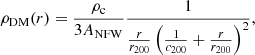 (18)
(18)
where ANFW can be written as
 (19)
(19)
Density profile uncertainties were computed from Montecarlo runs accounting for one-sigma error bars from our fit and those from the parameters in Girelli et al. (2020) and Child et al. (2018).
In Fig. 19 we display the cumulative baryonic (stellar plus black hole) and dark matter mass profiles from our fiducial fit to NGC 1277. We include 95.4% confidence interval (two sigma) bands for both profiles. Since the fDM(6 kpc) probability distribution peaks at zero (the border of the fitting interval) we calculated the confidence intervals as the 95.4 percentile rather than the interval between the 2.3 and the 97.7 percentiles. We also display the predicted dark matter halo profiles for freezing redshifts zf = 0 − 0.2 (meaning that the evolution of the galaxy has continued to the present, undergoing no freezing) and zf = 2.5 − 3, as well as the 95.4% confidence intervals based on the Montecarlo simulations. The predicted dark matter halo profiles for both freezing redshifts are very similar because the stellar mass of NGC 1277 roughly corresponds to that where the SHMR for all the redshifts intersect (Fig. 8 in Girelli et al. 2020).
 |
Fig. 19. Three-dimensional cumulative mass profiles of NGC 1277 for the baryonic component (stars plus black hole, in purple), the fitted dark matter halo (in black), and the predicted dark matter halo profiles for two different freezing redshifts (in blue and red for low and high zf, respectively) based on the SMHR parametrisation by Girelli et al. (2020) and the dark matter halo parametrisation by Child et al. (2018). The bands correspond to 95.4% confidence intervals. The baryonic component can be further subdivided into the black hole (dotted purple line) and the stellar component (dashed purple line). The grey vertical line indicates r = 6 kpc (18″), that is the radius within which we have kinematic data. |
The cumulative mass profiles in Fig. 19 indicate that within 6 kpc (equivalent to 5Re, which is the radius traced by our kinematic data), NGC 1277 has a mass-follows-light behaviour, with a maximum allowed dark matter fraction (at a two-sigma level) of fDM(6 kpc) = 0.05. This is in tension with fDM(6 kpc) = 0.09 predicted for both freezing redshifts zf = 0 and zf = 3. However, it is compatible with the minimum two-sigma mass fractions allowed by the models according to our Montecarlo runs based on the Girelli et al. (2020) and Child et al. (2018) works (fDM(6 kpc) = 0.03). The negligible amount of dark matter within 6 kpc, and hence the tension between the fit and the expectations, is a common feature among all the experiments listed in Table 3. Our results are compatible with those from Yıldırım et al. (2015), who found a fraction of dark matter within the effective radius, fDM(Re) compatible with zero.
The discrepancy between the fitted and the expected dark matter fraction for NGC 1277 arises from a combination of several factors. The extreme compactness of NGC 1277 might make it baryon-dominated over most of the disc, so it may become hard to characterise the dynamical effects of the underlying dark matter distribution. Also, the reported formal error bars ignore the systematics that might be introduced by the hypotheses used in the Jeans modelling (such as the use of a single mismatch parameter across the whole galaxy). However, those systematics are probably small because if the fitted parameters are robust against changes in the assumed velocity ellipsoid (as it occurs for fDM(6 kpc)), they can be assumed to be reliable (Cappellari 2020). The result is also robust against changes in the positioning of the galaxy centre and the estimated distance.
Contrary to the case of NGC 1277, Fig. 20 shows that the dark matter profile obtained in our fiducial fit of NGC 1278 falls right on top of the zf = 0 prediction. The fitted dark matter profile is above, but still compatible, with what would be expected for a zf = 3 galaxy. For NGC 1278, fDM(6 kpc) varies with the varying fitting approaches. Nevertheless, regardless of the fitting approach and other input parameters (such as the position of the centre of the galaxy and the estimated distance), we always find that NGC 1278 has a non-negligible dark matter fraction.
 |
Fig. 20. Same as Fig. 19, but for NGC 1278. The dashed grey line indicates the radius out to which we have kinematic data, that is 10 kpc or 30″. |
In summary, we find that the fact that the extreme relic galaxy NGC 1277 has no detectable dark matter within five effective radii is in tension with the expectations from models. On the other hand, we find that the regular massive ETG NGC 1278 has a detectable dark matter halo which is compatible with the models.
5.3. The dark matter fraction within one and five effective radii and within 6 kpc
In this section, we compare the fitted dark matter fractions of NGC 1277 and NGC 1278 with those of other massive ETGs from the literature, as well as with expectations from combining theoretical models with measurements of the sizes of massive ETGs. Our deep observations allow us to explore as far as 5 Re for NGC 1277 and 2.5 Re for NGC 1278. However, studies of large samples (e.g. Cappellari et al. 2013a; Santucci et al. 2022), typically only cover the central regions of the galaxies. Thus, here we compare the dark matter fractions within Re, fDM(Re). Given the small radius probed by these studies and the increased fraction of baryons as we approach the central regions of galaxies, this dark matter fraction comparison is of limited interest because these previous studies sampled radii where dark matter usually plays a minor role.
In Fig. 21, we compare the dark matter fractions fDM(Re) for NGC 1277 and NGC 1278 to the values obtained for a sub-sample of 103 galaxies from the ETG survey ATLAS3D (Cappellari et al. 2011) shown in the top panel of Fig. 10 from Cappellari et al. (2013a) and a sample of 161 passive galaxies from the SAMI Galaxy Survey (Croom et al. 2012; Bryant et al. 2015) shown in Fig. 7 from Santucci et al. (2022). The former data points correspond to the fits deemed to be good by the authors and come from JAM models similar to ours. The stellar masses of the galaxies from Santucci et al. (2022) were positively shifted by 0.23 dex to convert their assumed Chabrier (2003) IMF into a Salpeter (1955) one as we do in Sect. 3.2. Figure 21 also shows two M⋆ − fDM(Re) relations derived from the above-mentioned works. The green line comes from the lower panel in Fig. 10 in Cappellari et al. (2013a), and was derived from JAM fits where the NFW halo parameters were fixed to cosmologically motivated values obtained from Moster et al. (2010). The red line indicates the fit from Fig. 7 in Santucci et al. (2022) and is again shifted by 0.23 dex.
 |
Fig. 21. Dark matter fraction within the effective radius, fDM(Re), as a function of the stellar mass for NGC 1277 and NGC 1278 (star symbols). The error bars represent one sigma confidence intervals (that corresponding to NGC 1277 is smaller than the symbol size). Circles correspond to the 103 ATLAS3D galaxies with good fits in Cappellari et al. (2013a) and the diamond symbols correspond to the data for a sample of 161 passive galaxies from the SAMI Galaxy Survey from Santucci et al. (2022). The colour coding of the symbols indicates the effective radius of the galaxies as shown by the side-bar. The ATLAS3D data points were derived by merging the galaxy distances from Cappellari et al. (2011), the effective radii and luminosities from Cappellari et al. (2013a), and the fDM(Re) and Υ⋆ values from Cappellari et al. (2013b). The effective radii for the SAMI galaxies were kindly provided by G. Santucci. The green line indicates the M⋆ − fDM(Re) relation derived from JAM models with a fixed cosmologically motivated NFW dark matter halo from Cappellari et al. (2013a). The red line and confidence band correspond to the fit represented in Fig. 7 from Santucci et al. (2022). The black line shows a prediction of the M⋆ − fDM(Re) relation made by combining the dark matter haloes derived from the SHMR from Girelli et al. (2020) and the dark matter halo parametrisation from Child et al. (2018) with the Re values derived from a linear fit (Eq. (20)) to the size measurements for galaxies with a morphological type T ≤ −1 in Trujillo et al. (2020). The latter relation was calculated assuming a de Vaucouleurs (1948) profile for the stellar component and it is complemented by a one-sigma uncertainty band calculated using a Montecarlo simulation. For the Trujillo et al. (2020) and the Santucci et al. (2022) data and the Girelli et al. (2020) SHMR, the stellar masses were corrected by a factor 0.23 dex to convert the assumed Chabrier (2003) IMF into a Salpeter (1955) one (see Eq. (3) in Sect. 3.2). |
Figure 21 also displays a third M⋆ − fDM(Re) relation (black line) that was obtained from the dark matter haloes predicted by combining the SHMR from Girelli et al. (2020, which is corrected to a Salpeter IMF too) and the dark matter halo parametrisation from Child et al. (2018, see Sect. 5.2). In order to assign an effective radius to each galaxy stellar mass, we produced a linear fit between log Re and log M⋆ using the observational data for ETGs (Hubble-Reynolds type T ≤ 1) from Trujillo et al. (2020). After correcting M⋆ by 0.23 dex to shift the IMF to a Salpeter one, we obtained
 (20)
(20)
where Re is in kpc and M⋆ in M⊙. To estimate the fraction X⋆(r = Re) of the stellar mass that is found within a three-dimensional radius r = Re we assumed a Sérsic (1963) profile with an index n = 4 (a de Vaucouleurs 1948, profile). The fraction X⋆ for the n = 4 specific case was calculated by combining Eqs. (30) and (41) and from Baes & Gentile (2011)
![Mathematical equation: $$ \begin{aligned} X_\star (r) = 1.523\left(\frac{r}{R_{\rm e}}\right)^2G^{8,1}_{1,9}\left[\begin{array}{cc}0&\\ \boldsymbol{b},&-1\end{array}\left|0.7132\left(\frac{r}{R_{\rm e}}\right)^2\right.\right], \end{aligned} $$](/articles/aa/full_html/2023/07/aa46291-23/aa46291-23-eq68.gif) (21)
(21)
where G is the Meijer G function (Meijer 1936) and
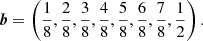 (22)
(22)
We found that for a de Vaucouleurs (1948) profile X⋆(Re) = 0.415. The M⋆ − fDM(Re) relation is complemented by a one-sigma uncertainty band that was calculated with a Montecarlo simulation using the uncertainties quoted by Girelli et al. (2020) and Child et al. (2018), as well as an intrinsic sigma of 0.057 in log Re from Table 3 in Trujillo et al. (2020).
We found that the fDM(Re) value for NGC 1278 is compatible with the M⋆ − fDM(Re) relation from Santucci et al. (2022). NGC 1278 is below the M⋆ − fDM(Re) relations from Cappellari et al. (2013a), but is within the scatter of the galaxies in the lower panel of their Fig. 10. NGC 1278 also falls below the two other M⋆ − fDM(Re) relations examined in Fig. 21. The fact that NGC 1278 falls below all the M⋆ − fDM(Re) relations while it has a dark matter halo compatible with the expectation for its mass (Fig. 20) is because its effective radius (Re = 4.2 kpc) is smaller than the average for ETGs of its mass (Re = 7.6 kpc from Eq. (20)).
NGC 1277 is well below the three M⋆ − fDM(Re) relations shown in Fig. 21 with fDM(Re) < 0.005 (95.4% confidence interval). Based on the M⋆ − fDM(Re) relation that we established using models and the effective radii in Trujillo et al. (2020), the expected dark matter fraction of a galaxy with the stellar mass of NGC 1277 is 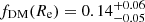 at a one-sigma confidence level and
 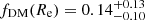 at a two-sigma confidence level. Calculating fDM(Re) is another way of demonstrating the dark matter deficient nature of this object in comparison with other galaxies with a similar stellar mass. However, as NGC 1277 is very compact, we emphasise that its extreme lack of dark matter is only fully demonstrated by finding little to no dark matter within 6 kpc (5 Re).
If two galaxies have the same dark matter halo and the same stellar mass, the most compact one has the smallest fDM(Re). We colour-coded the symbols in Fig. 21 according to their Re to check whether galaxies with a small fDM(Re) are exclusively compact (Re ≈ 1 kpc). We find that galaxies with a small fDM(Re) can be relatively extended (with effective radii of a few kpc), and that some compact galaxies have a non-negligible central dark matter fraction. Therefore, the reason why Cappellari et al. (2013a) and Santucci et al. (2022) find galaxies with fDM(Re)≈0 cannot be solely the compactness of the objects. Instead, these small fDM(Re) values are likely because the fraction of dark matter within 1 Re is so small, that it becomes hard to constrain it. Indeed, ATLAS3D was designed to observe galaxies out to 1 Re (Cappellari et al. 2011) and most of the Santucci et al. (2022) galaxies are covered out to less than 2 Re (see their Fig. 1). Figure 4 in Cappellari et al. (2015) illustrates this point by showing that, whereas the stellar and the total mass profiles of massive ETGs do not differ much in the inner 1 Re, the stellar density profile falls much faster than the total one in the outskirts. Hence, our large radial coverage (5 Re for NGC 1277 and 2.5 Re for NGC 1278) ensures a precision in the characterisation of the dark matter component that cannot be achieved if we are limited to the inner 1 − 2 Re.
To stress the importance of the fact that we find little to no dark matter within 5 Re for NGC 1277, in Fig. 22 we compare the properties of NGC 1277 with a M⋆ − fDM(5 Re) relation computed by combining the works by Child et al. (2018), Girelli et al. (2020), and Trujillo et al. (2020) as done for the M⋆ − fDM(Re) relation in black in Fig. 21. This time the fraction of the stellar mass lying within the radius of interest is X⋆(5 Re) = 0.842. Additionally, we used a Montecarlo simulation to estimate confidence intervals, yielding  (at a 68.3% confidence interval) and
 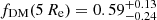 (at a 95.4% confidence interval) for an ETG with the stellar mass of NGC 1277. This is clearly incompatible with the two-sigma limit fDM(5 Re) < 0.05 obtained from our dynamical fit (Sect. 5.2).
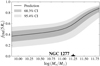 |
Fig. 22. Dark matter fraction within five effective radii fDM(5 Re) for NGC 1277 (star) with the 95.4% confidence interval indicated by a vertical line. The black line indicates the predicted M⋆ − fDM(5 Re) relation based on the dark matter haloes profiles and Re values derived as in Fig. 21. The grey shades indicate the 68.3% (darker) and 95.4% (lighter) confidence intervals of the relation calculated using a Montecarlo simulation. A de Vaucouleurs (1948) profile was assumed for the stellar density profile of the galaxies. |
As NGC 1277 is very compact compared to a typical galaxy of its mass (1.2 kpc versus 5.5 kpc from the M⋆ − Re relation derived from Trujillo et al. 2020), the lack of dark matter within 5 Re could be interpreted as a consequence of the high density of the stellar component. To emphasise that NGC 1277 is genuinely dark matter deficient, the dark matter fraction within a given physical radius could be checked instead. In Fig. 23 we compare fDM(6 kpc) for NGC 1277 and NGC 1278 with that of a prediction calculated as for Figs. 21 and 22. Here, X⋆(6 kpc) had to be computed in a stellar mass by stellar mass basis, as this fraction varies as a function of 6 kpc/Re. We again show that, whereas NGC 1278 falls within the expected trend, NGC 1277 is below it. Although the discrepancy between the fit and the prediction is not as large as for the M⋆ − fDM(5 Re) relation, a tension is still found (fDM(6 kpc) < 0.05 two-sigma limit versus fDM(6 kpc) = 0.16 ± 0.05 and fDM(6 kpc) = 0.16 ± 0.10 at 68.3% and 95.4% confidence intervals, respectively).
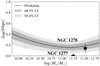 |
Fig. 23. Same as Fig. 22, but this time for the dark matter fraction enclosed within 6 kpc, fDM(6 kpc), and including the data point corresponding to NGC 1278. |
The tension between the measured dark matter fraction and the predictions would pose a challenge for ΛCDM if NGC 1277 were found to be incompatible with being a statistical outlier. According to Quilis & Trujillo (2013), relic galaxies (defined as those that have grown less than 10% in mass through mergers) are expected to be today one in one thousand among massive galaxies with M⋆ > 8 × 10¹⁰ M⊙. Assuming a normal distribution, relic galaxies would be 3.3-σ outliers of the distribution. If we use this number to gauge the level of tension between the measured dark matter fraction in NGC 1277 and that predicted from the simulations, we find that the answer depends on whether the dark matter fraction is measured within a given physical scale or within a given number of effective radii. Whereas in the former case NGC 1277 might be compatible with being a statistical outlier (the upper two-sigma limit of the dark matter fraction in NGC 1277 is close to the lower two-sigma limit of the expectation), in the latter one there is a strong (more than 5σ) tension. Given that we lack a clear-cut answer about the relevant radius within which the dark matter fraction should be measured, we are refraining from speculating whether the tension observed for NGC 1277 challenges the current cosmological paradigm.
The decaying rotation curve of NGC 1277 (Fig. 7) bears a qualitative resemblance with those of the high-redshift massive star-forming galaxies studied by Genzel et al. (2017). The latter six galaxies are also found to be dark matter-poor, with fDM(Re)≲0.2 and compatible with zero in four cases. However, these galaxies cannot be straightforwardly compared to NGC 1277. The reason is that the typical effective radius in the Genzel et al. (2017) sample is Re ≈ 8 kpc, so these objects are not nearly as compact as NGC 1277. Also, in five out of six galaxies, the data coverage stops at R ≈ 2 Re, so it misses the galactic outskirts where dark matter is presumed to be playing a major role and might be able to provide tight constraints on fDM(Re).
In conclusion, we find that NGC 1277 lacks dark matter within 1 Re, 5 Re, and 6 kpc when compared to the expectations from models. On the other hand, we find that NGC 1278 behaves according to what is expected for a massive ETG.
5.4. How could a compact dark matter-deficient galaxy form?
We have found evidence that, in addition to being the best massive relic candidate in the local Universe, NGC 1277 is dark matter deficient (it has a fraction of dark matter within 5 Re of less than 5% at a two sigma confidence level, whereas the expected value is ∼60%; Sect. 5.3 and Fig. 22). The principle of parsimony suggests that the two oddities have a common cause (or that one is the consequence of the other). However, another relic, Mrk 1216 (Ferré-Mateu et al. 2017), has been found to contain a significant fraction of dark matter within Re (Yıldırım et al. 2015; Buote & Barth 2019). The situation poses a conundrum: either (1) relic galaxies can form with largely different dark matter contents, or (2) NGC 1277 and Mrk 1216 are different kinds of objects born and/or evolved under different circumstances. The latter possibility is supported by the work by Ferré-Mateu et al. (2017), who found Mrk 1216 to be the galaxy with the smallest ‘degree of relic’ (that is, the one that is the most similar to a regular ETG) among their three-galaxy sample (which includes NGC 1277). They also found that the burst of star formation that generated the bulk of the baryonic mass in Mrk 1216 was more extended in time than for the other galaxies in the sample, as well as traces of recent accretion. As a consequence, they posit that Mrk 1216 is a relic that is on its way to become a ‘regular’ massive ETG (see also Yıldırım et al. 2015).
How did NGC 1277, one of the densest known galaxies, form within a not so dense dark matter halo? This seems counterintuitive and, according to a study by Flores-Freitas et al. (2022) based on the TNG50 cosmological simulation (Pillepich et al. 2019; Nelson et al. 2019), the progenitors of present-day massive relic galaxies inhabited at z ∼ 4 dark matter haloes that were more massive than those of an average quiescent galaxy progenitor with a similar stellar mass. Also, Fig. 7 in Lapiner et al. (2023) shows that simulations predict that even the most compact blue nuggets have non-negligible dark matter fractions (fDM(Re)≳0.1).
If it is possible for a few rare galaxies not to have dark matter, it becomes easy to explain why they do not undergo the envelope accretion phase. In the absence of a halo, nearby galaxies undergo parabolic flybys instead of spiralling-in due to dynamical friction (Chandrasekhar 1943). This hypothesis would hold even if we had underestimated fDM(5 Re), because the stripping of the outskirts of the halo (see discussion below) would still be a plausible mechanism to explain the lack of accretion. On the other hand, regular massive ETGs like NGC 1278 are effective at cannibalising small dark matter rich-galaxies, which impacts both Re and fDM (e.g. Hilz et al. 2012; Tortora & Napolitano 2022). If we assume that the lack of an envelope in NGC 1277 is due to a dark matter deficiency, it must have either lost its dark matter early (before significant accretion occurred) or was dark matter deficient ab initio. Hence, the big question about NGC 1277 shifts from ‘how did it avoid to accrete an envelope?’ to ‘why is it dark matter deficient?’.
If dynamical friction were suppressed in NGC 1277, it would be extremely unlikely that its central black hole were accreted as suggested by Shields & Bonning (2013). The relatively large mass of the central black hole in NGC 1277 should be then attributed to the fact that the black hole-related scaling relations are established based on galaxies that have accreted an envelope. Indeed, present-day regular massive ETGs are significantly more massive than they were in their blue nugget phase.
A possible way to generate a dark matter-poor galaxy that resembles a massive relic was proposed by Flores-Freitas et al. (2022). They used the TNG50 cosmological simulation to identify five relic analogues, of which the one residing in subhalo 6 is the purest and the most similar to NGC 1277. The simulated galaxy is born in isolation within a massive ∼1012 M⊙ dark matter halo that is significantly stripped as it enters a cluster. As the galaxy loses most (∼90%) of its dark matter, it also leaves behind most of its gas, which prevents further star formation from happening. During this process, the stellar body of the galaxy remains mostly intact, as it loses only about 20% of its mass. The resulting galaxy has 1.4 times more mass in dark matter than in stars (Flores-Freitas et al. 2022), and virtually all the dark matter outside a radius of 30 kpc has been stripped away (Flore-Freitas, priv. comm.). This phenomenon is similar to the stripping of dark matter of satellites as they interact with their main galaxy (Engler et al. 2021). Moreno et al. (2022) also explored simulated dwarf satellite galaxies that lose most of their dark matter as they have a close interaction with their parent galaxy. They proposed that in such events the stellar component is harder to remove than the dark matter one because stellar orbits are more circular than those of dark matter particles. Hence, repeated interactions would be efficient at stripping dark matter particles when they are close to their apocentre.
The main caveat of the Flores-Freitas et al. (2022) scenario is given by the authors themselves. Indeed, as subhalo 6 falls within the cluster, the apparent stripping might in part be caused by some of the material being assigned to the parent halo. Thus, the mass loss could be an artefact introduced by the algorithm assigning particles to the different dark matter haloes. Another problem is that, whereas the outer parts of the halo are efficiently stripped, the dark matter mass within the inner 6 kpc diminishes by a factor of less than two (Flores-Freitas; priv. comm.), so the mechanism does not seem sufficient to remove most of the dark matter from the central parts of the galaxy. On the other hand, the stripping of the outer parts of the halo would probably be sufficient to greatly reduce dynamical friction and perhaps prevent the accretion of an envelope. A possible way around all these caveats is that subhalo 6 contains the best relic analogue within the TNG50 volume, but this volume of 1.4 × 10⁵ Mpc3 is relatively small compared to the observed local number density of relics (three in 5 × 10⁶ Mpc3; Ferré-Mateu et al. 2017) and might be insufficient to cover the most rare and extreme objects.
A scenario similar to that put forward by Flores-Freitas et al. (2022) was given by Yu et al. (2018). These authors studied the Illustris simulation (Vogelsberger et al. 2014) searching for dark matter-deficient galaxies. They found a galaxy akin to NGC 1277 that is, compact (Re ≈ 2 kpc), massive (M⋆ = 9.42 × 10¹⁰ M⊙), and with a total dark matter mass fraction below 0.1. According to Yu et al. (2018), a strong interaction with the environment at redshift z < 1 would have stripped about half of the stars from the galaxy and most of the dark matter (their Fig. 2). The result would be a dense compact galaxy with little dark matter. Only one such galaxy is found within the (106.5 Mpc)3 ≈ 1.2 × 10⁶ Mpc3 Illustris box, which is tantalisingly close to the observational density constraints by Ferré-Mateu et al. (2017) and of the same order of magnitude as the number density of relics estimated by Quilis & Trujillo (2013). It is also compatible with the estimated density of massive ultra-compact galaxies for the z < 0.3 Universe of (1.0 ± 0.4)×10−6 Mpc−3 from Buitrago et al. (2008) and the lower limit for the relic density of one relic within 107 Mpc3 from Spiniello et al. (2021b).
A possible caveat of the work by Yu et al. (2018) is that the Illustris simulation yields lower dark matter fractions for ETGs than those measured through gravitational lensing (Mukherjee et al. 2022). Another caveat is that, since the mass loss in their scenario occurred quite late (z < 1), the interaction should have stripped both the envelope and the population of blue globular clusters (discovered to be absent in Beasley et al. 2018). This possibility is discussed in Beasley et al. (2018) and found to be unlikely because, whereas tidal stripping could explain the lack of an envelope, it could not explain the extreme density of the centre of the galaxy. As a consequence, they conclude that NGC 1277 was already dense and compact at birth. Another sign that NGC 1277 never had a significant envelope can be found by comparing this galaxy with the regular ETG NGC 1278. Indeed, we find that NGC 1278 has signs of a relatively young (< 10 Gyr) accreted stellar population all the way to its centre (Ferré-Mateu et al., in prep.) which should be observed in NGC 1277 too if it ever had an envelope that was later lost. Furthermore, NGC 1277 lacks shells and streams down to μr = 26.8 mag arcsec−2 (implying that no more than 2% of the stellar mass of the galaxy is missing from the deepest HST imaging; Trujillo et al. 2014). This indicates a paucity of interactions affecting the stellar component in the last few Gyr (Mancillas et al. 2019). Within the framework of the two-phase formation scenario the simplest way to reconcile the stripping hypothesis with the observations is by assuming that the dark matter loss occurred very early (as seen in the work by Flores-Freitas et al. 2022), before NGC 1277 had time to accrete a significant envelope.
In a bottom-up hierarchical paradigm, galaxies grow by mergers. In the early Universe, galaxies were richer in gas than nowadays and mergers and cold streams caused a wet compaction that led to the formation of the compact high-redshift galaxies known as blue nuggets (e.g. Lapiner et al. 2023). It is possible that for a few major mergers the geometry of the encounter (impact parameter and relative velocity) were such that the collisionless dark matter would escape the system. The escape velocity from a 1011 M⊙ body at a distance of 1 kpc is ≈1000 km s−1, so under this hypothesis the relative velocity of the two bodies should be of the order of 2000 km s−1 in order to remove the dark matter from the system. Whereas these relative velocities can hardly be found in the field, they are consistent with the high-velocity tail within rich clusters. For example the Perseus cluster where NGC 1277 resides, is a rich cluster (Völk & Atoyan 2000) with a velocity dispersion of  km s−1 (Girardi et al. 1993). Hence, we speculate that infrequent high-velocity collisions during the proto-cluster phase are possible. Indeed, assuming a Hubble-Lemaître parameter at z = 2, H(z = 2)≈200 km s−1, we obtain from the relations in Ferragamo et al. (2022) that to reach a velocity dispersion of 1000 km s−1 (so a few outliers have velocities of 2000 km s−1), a cluster mass of 3 × 10¹⁴ M⊙ is sufficient. This mass is less than half the current mass of the Perseus cluster, M = 8.5 × 10¹⁴ M⊙ (Mathews et al. 2006).
In this high-velocity collision scenario, the situation would be somewhat similar to that of the Bullet Cluster (Clowe et al. 2004; Markevitch et al. 2004), where dissipative matter (gas) is left behind. However, the analogy cannot be pushed too far because the gas in the blue nugget progenitor fragments would be orders of magnitude denser and cooler than that in the intra-cluster medium.
In the high-velocity encounter framework, the difference between the progenitor of NGC 1277 and that of a blue nugget on its way to become a regular ETG would be that the latter keeps most of its dark matter. This might be because the mergers that generated the progenitors of regular ETGs were mostly minor (as suggested by Zolotov et al. 2015) or because the relative velocity of the merging fragments was not large enough to prevent the dark matter from falling back.
The high-velocity merger hypothesis has of course several caveats. The first one is that NGC 1277 looks like the passively evolved product of the average blue nugget which is presumed to have a regular fraction of dark matter. As a consequence, if our suggestion is valid, young massive ETGs should look similar irrespective of their dark matter content. This is not completely unreasonable because the dark matter fraction in the central regions of blue nuggets and massive ETGs is often small (Lapiner et al. 2023, and Fig. 21, respectively). However, it remains to be seen whether the lack of a dense extended dark matter halo would not result in the loss of many of the baryons at the onset of intense star formation. Another problem of this scenario is related to the time-scales involved in the process. On one hand, intense star formation would likely be triggered by the collision. On the other hand, the star formation time-scale should be longer than the dynamical time-scale (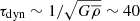 Myr, where
  is the average density of NGC 1277) for the gas to have time to settle in a disc in order to produce a mostly rotation-supported stellar body. Also, the density of the gas should have been high enough to ensure a fast cooling to prevent the escape of a large fraction of the gas shock-heated by the collision.
A third possibility to explain the apparent lack of dark matter in NGC 1277 is a strong departure from a NFW dark matter profile. Our data do not reach the depth required to probe the matter distribution beyond 6 kpc. This leaves the door open for a halo with a core much flatter than that predicted by a NFW profile. It is known that density fluctuations introduced by AGN and stellar feedback at the centre of galaxies can erase cusps (e.g. Martizzi et al. 2013). The extremely massive central black hole could have powered the feedback, but such processes are also efficient at expelling baryons, so they should have occurred after most of the gas was transformed into stars. Therefore it is unclear how an extremely concentrated stellar component could sit within a halo that is more cored than average unless a large amount of fresh gas were accreted after the AGN had modified the density profile. Furthermore, a cored halo would not prevent dynamical friction from happening, so it would fail to naturally explain the absence of an envelope. In this case, the lack of mergers would be the consequence of a fortuitous lack of nearby galaxies to interact with.
Finally, a mass-follows-light scenario could be considered. In this case the dark matter distribution would be similar to that of the baryons. The presence of dark matter would be observed as an increase in the mass-to-light ratio, which would manifest as a large mismatch parameter α and mimicking a bottom-heavy IMF. At first glance the high value of α for NGC 1277 makes this explanation plausible. However, the dynamically estimated mass-to-light ratio broadly agrees with that that can be extracted from the line-strength index-based study by Martín-Navarro et al. (2015). The fact that a bottom-heavy IMF is found using two completely independent methods leaves little room for a significant mass-follows-light dark matter component.
One might be tempted to use the fact that NGC 1277 lacks detectable dark matter to speculate about the (in)existence of Milgromian dynamics (also known as MOND; Milgrom 1983) or other alternatives to the ΛCDM paradigm. Given a centrally concentrated baryonic mass of M⋆ ≈ 1.6 × 10¹¹ M⊙ and an acceleration constant a0 = 1.24 × 10⁻¹⁰ m s−2 (McGaugh 2011), a radius R = 13 kpc should be explored to be able to probe the fully Milgromian regime. This is about twice the radius that we cover and therefore our data do not permit studying the Milgromian regime unless the Newtonian-Milgromian transition were not abrupt. In a Milgromiam framework the lack of dark matter could not be invoked to explain the absence of dynamical friction and the missing envelope and, as in the case of the cored halo discussed above, the lack of an envelope would have been caused by the paucity of mergers for this particular galaxy.
NGC 1277 is similar to a gigantic rotating globular cluster, where the stars are the main contributor to the mass. Our favoured hypothesis to explain the formation of such a peculiar object is that NGC 1277 was born with little dark matter or that it lost most of it very early at or soon after its blue nugget phase. A plausible mechanism for that is that most of the dark matter of the galaxy was lost through interactions as it entered and moved through the Perseus cluster. Alternatively, NGC 1277 could have formed in a high-velocity collision of gas-rich fragments, where baryons coalesced and formed stars as dark matter left the system because of a velocity exceeding the escape one.
6. Summary and conclusions
Relic galaxies are fascinating objects thought to be the frozen remains of the high redshift massive ETGs (z ≳ 2). Whereas according to the two-phase formation scenario for massive ETGs the vast majority of these objects have suffered a complex merger history and have accreted an envelope, relic galaxies are thought to be the relatively untouched and passively evolved descendants of the blue nuggets observed in the early Universe. Very few relic galaxies are known, the most pristine of which is NGC 1277 (Trujillo et al. 2014). NGC 1277 is a massive (stellar mass M⋆ ≈ 1.8 × 10¹¹ M⊙) and centrally concentrated (effective radius Re ≈ 1.2 kpc) galaxy in the Perseus cluster.
We have revisited NGC 1277 using data from the fibre spectrograph GCMS at the 2.7 m Harlan J. Smith telescope (Fig. 1). The data are of unprecedented interest because the long 2.5 h exposure allows us to study the outskirts of the galaxy (going from a radius of 13″ in literature studies up to 18″ here). The field of view also covers the regular massive ETG NGC 1278, a galaxy that constitutes an excellent benchmark against which to compare NGC 1277. In order to complement the GCMS data of NGC 1277, we use kinematics of the innermost  of the galaxy obtained by Walsh et al. (2016) using the AO-assisted NIFS integral field spectrograph.
Our aim was to produce dynamical models of both NGC 1277 and NGC 1278 and recover their mass distribution. We used HST images to compute colour-derived mass density maps to be able to disentangle the dark and the baryonic matter. Both the surface brightness and the surface density maps were parametrised using multi-Gaussian expansions (MGEs; Tables 1 and 2 and Figs. 10 and 11) produced with the code by Cappellari (2002).
We fitted the  maps of the two galaxies (Figs. 2 and 3) by feeding Jeans anisotropic models provided by JAM (Cappellari 2008, 2020) into the adamet Bayesian analysis code (Cappellari et al. 2013a). For each galaxy, we fitted (among other parameters) the mismatch parameter indicating how the mass-to-light ratio compares to that expected from a Salpeter (1955) IMF, α, and the dark matter fraction within 6 kpc, fDM(6 kpc). The 6 kpc radius matches the maximum coverage of the good-quality GCMS data of NGC 1277 and corresponds to five effective radii (5 Re) for this particular galaxy. During the fitting process we assumed that the galaxies are axisymmetric and that they have a single mismatch parameter throughout their stellar body.
Our fits (Figs. 12 and 13) show that NGC 1277 has a large mismatch parameter α ≈ 1.34, which is a consequence of a bottom-heavy IMF. Our most surprising result is that there is little to no dark matter within the explored radius and that the maximum permissible dark matter fraction within 6 kpc (corresponding to 5 Re) is fDM(6 kpc) = 0.05 (95.4% confidence interval; Fig. 19), which is in tension with the fDM(6 kpc) = 0.09 expectation based on the ΛCDM cosmology as obtained from stellar-to-halo mass relations by Girelli et al. (2020) and the dark matter halo radial profile parametrisation in Child et al. (2018). This low dark matter fraction is on an even stronger tension with the prediction of fDM(5 Re)∼0.6 (Fig. 22) obtained from combining the above two works with a M⋆ − Re relation for massive ETGs extracted from the data in Trujillo et al. (2020).
NGC 1278 has a mismatch parameter α ≈ 1.16, which indicates a shallower IMF slope than for NGC 1277 (Fig. 16). According to our fiducial fit, the dark matter fraction of NGC 1278 is fDM(6 kpc) = 0.14 ± 0.08 (95.4% confidence interval), which which agrees with the expectations from the ΛCDM cosmology (Fig. 20).
The large mismatch parameter of NGC 1277 indicates a high value of the stellar mass-to-light ratio, Υ⋆r = 7.0 M⊙/L⊙r. This provides a dynamically derived constraint to the IMF that is compatible with the bottom-heavy IMFs determined by Martín-Navarro et al. (2015) and Ferré-Mateu et al. (2017) using line-strength indices (Fig. 18).
The lack of a dynamically significant dark matter component in NGC 1277 confirms the findings by Yıldırım et al. (2015). The fact that one of the galaxies with the densest stellar component lies within an underdense dark matter halo is extremely puzzling. On the other hand it explains why it has not accreted an envelope, since the lack of an extended dark matter component would shut down dynamical friction and hence the spiralling down of nearby dwarf galaxies. Hence, we propose that NGC 1277 either lost its dark matter early, before it accreted a significant envelope, or was dark matter deficient ab initio.
A possible way to create a dark matter-poor object such as NGC 1277 has been proposed by Flores-Freitas et al. (2022) who, based on the TNG50 simulation, posited that relic galaxy analogues may have lost a large fraction of their dark matter through interactions with the environment as they entered a cluster. A similar scenario has been proposed by Yu et al. (2018) based on a search for dark matter deficient galaxies in the Illustris simulation. It is suggestive that the density of compact, massive and dark matter deficient galaxies in the Illustris simulation is very close to that found in the local Universe by Ferré-Mateu et al. (2017, one in ≈1.2 × 10⁶ Mpc3 versus three in ≈5 × 10⁶ Mpc3) and compatible with other density estimates by Buitrago et al. (2018) and Spiniello et al. (2021b). Simulations have also shown a similar mechanism at work for dwarf galaxies through interactions with their parent galaxies (Engler et al. 2021; Moreno et al. 2022). Alternatively, an NGC 1277-like object could have been born in a high-velocity collision of gas-rich objects where dark matter would have escaped the system leaving behind a rotating stellar body (blue nugget). The high relative velocities required for this process to work could only be found in a cluster-like environment and, based on Ferragamo et al. (2022), we speculate that they might have been possible in the progenitors of the rich galaxy clusters at z ∼ 2.
We have found that NGC 1277 lacks any detectable dark matter within 6 kpc (corresponding to five effective radii, 5 Re) of its centre. Massive dark matter-deficient galaxies are unexpected within the framework of the consensus cosmological model ΛCDM. We propose that the galaxy was dark matter deficient ab initio or soon after birth and that the relic nature of NGC 1277 stems from the lack of an extended halo. In order to confirm this hypothesis more deep integral field studies of pure relic galaxies are required. It would also be interesting to check whether even deeper observations of NGC 1277 can find traces of a tenuous dark matter halo by finding a flattening of the rotation curve at a radius R ≳ 10 kpc.
We used v6.3.2 of the Python package JamPy, available from https://pypi.org/project/jampy/
The software can be obtained from http://p3d.sourceforge.io
We used v7.4.5 of the pPXF package available from https://pypi.org/project/ppxf/
The E-MILES spectral energy distribution libraries can be downloaded from http://research.iac.es/proyecto/miles/pages/spectral-energy-distributions-seds/e-miles.php
We used v2.0.7 of the Python package adamet, available from https://pypi.org/project/adamet/
The HyperLeda database is hosted at http://leda.univ-lyon1.fr/
We used v5.0.14 of the MgeFit Python package from https://pypi.org/project/mgefit/
We used v6.3.2 of the Python package JamPy, available from https://pypi.org/project/jampy/
The E-MILES spectral energy distributions can be downloaded from http://research.iac.es/proyecto/miles/pages/photometric-predictions-based-on-e-miles-seds.php
Acknowledgments
We thank the referee, Dr. Eric Emsellem, for his very helpful comments that have helped strengthen this article. We thank Giulia Santucci for kindly sharing information about Fig. 7 in Santucci et al. (2022). We thank Rodrigo Flores-Freitas and Ana L. Chies-Santos for sharing valuable insights about the intricacies of their work in Flores-Freitas et al. (2022). We thank Michalina Maksymowicz-Maciata for her careful reading of the paper that has led to the discovery of a couple of typos. S.C. is indebted to all the participants at the ‘Cosmic nuggets – A feast of compact and massive Galaxies across the Universe’, in particular Dr. Claudia Pulsoni, for the useful idea exchanges and for the references that were essential for the discussion in this paper. S.C. also thanks Drs. Jorge Sánchez Almeida, Alexandre Vazdekis, Claudio dalla Vecchia, and Tod Lauer for useful comments and enlightening discussions. S.C. and M.A.L.L. acknowledge support from the Ramón y Cajal programme funded by the Spanish Government (references RYC2020-030480-I and RYC2020-029354-I). S.C. acknowledges funding from the State Research Agency (AEI-MCINN) of the Spanish Ministry of Science and Innovation under the grants ‘The structure and evolution of galaxies and their central regions’ with reference PID2019-105602GB-I00/10.13039/501100011033, and ‘Thick discs, relics of the infancy of galaxies’ with reference PID2020-113213GA-I00. I.T. acknowledges support from the ACIISI, Consejería de Economía, Conocimiento y Empleo del Gobierno de Canarias and the European Regional Development Fund (ERDF) under grant with reference PROID2021010044 and from the State Research Agency (AEI-MCINN) of the Spanish Ministry of Science and Innovation under the grant PID2019-107427GB-C32 and IAC project P/300624, financed by the Ministry of Science and Innovation, through the State Budget and by the Canary Islands Department of Economy, Knowledge and Employment, through the Regional Budget of the Autonomous Community. F.B. also acknowledges support from the grants PID2020-116188GA-I00 and PID2019-107427GB-C32 by the Spanish Ministry of Science and Innovation. M.A.L.L. acknowledges support from the Spanish grant PID2021-123417OB-I00. A.F.M. has received support from the Spanish Ministry grants CEX2019-000920-S, PID2021-123313NA-I00 and RYC2021-031099-I. This research was supported by the International Space Science Institute (ISSI) in Bern, through ISSI International Team project No. 505 (The Metal-THINGS Survey of Nearby Galaxies). Based on observations made with the NASA/ESA Hubble Space Telescope, and obtained from the Hubble Legacy Archive, which is a collaboration between the Space Telescope Science Institute (STScI/NASA), the Space Telescope European Coordinating Facility (ST-ECF/ESA) and the Canadian Astronomy Data Centre (CADC/NRC/CSA). This research has made use of the NASA/IPAC Extragalactic Database (NED), which is funded by the National Aeronautics and Space Administration and operated by the California Institute of Technology. We acknowledge the usage of the HyperLeda database (http://leda.univ-lyon1.fr). This research made use of NumPy (Harris et al. 2020), SciPy (Virtanen et al. 2020), SymPy (Meurer et al. 2017), and Astropy (http://www.astropy.org) a community-developed core Python package for Astronomy (Astropy Collaboration 2013, 2018). This research made use of Photutils, an Astropy package for detection and photometry of astronomical sources (Bradley et al. 2022). This research was partially based on data from the MILES project. This research has made use of the integral-field spectroscopy data-reduction tool P3D, which is provided by the Leibniz-Institut für Astrophysik Potsdam (AIP).
References
- Ahumada, R., Prieto, C. A., Almeida, A., et al. 2020, ApJS, 249, 3 [Google Scholar]
- Astropy Collaboration (Robitaille, T. P., et al.) 2013, A&A, 558, A33 [NASA ADS] [CrossRef] [EDP Sciences] [Google Scholar]
- Astropy Collaboration (Price-Whelan, A. M., et al.) 2018, AJ, 156, 123 [Google Scholar]
- Auger, M. W., Treu, T., Brewer, B. J., & Marshall, P. J. 2011, MNRAS, 411, L6 [Google Scholar]
- Baes, M., & Gentile, G. 2011, A&A, 525, A136 [NASA ADS] [CrossRef] [EDP Sciences] [Google Scholar]
- Bai, L., Yee, H. K. C., Yan, R., et al. 2014, ApJ, 789, 134 [NASA ADS] [CrossRef] [Google Scholar]
- Baldry, I. K., Sullivan, T., Rani, R., & Turner, S. 2021, MNRAS, 500, 1557 [Google Scholar]
- Barbosa, C. E., Spiniello, C., Arnaboldi, M., et al. 2021, A&A, 649, A93 [NASA ADS] [CrossRef] [EDP Sciences] [Google Scholar]
- Beasley, M. A., Trujillo, I., Leaman, R., & Montes, M. 2018, Nature, 555, 483 [NASA ADS] [CrossRef] [Google Scholar]
- Bilton, L. E., & Pimbblet, K. A. 2018, MNRAS, 481, 1507 [CrossRef] [Google Scholar]
- Bradley, L., Sipőcz, B., Robitaille, T., et al. 2022, https://doi.org/10.5281/zenodo.6825092 [Google Scholar]
- Bryant, J. J., Owers, M. S., Robotham, A. S. G., et al. 2015, MNRAS, 447, 2857 [Google Scholar]
- Buitrago, F., Trujillo, I., Conselice, C. J., et al. 2008, ApJ, 687, L61 [Google Scholar]
- Buitrago, F., Trujillo, I., Curtis-Lake, E., et al. 2017, MNRAS, 466, 4888 [NASA ADS] [Google Scholar]
- Buitrago, F., Ferreras, I., Kelvin, L. S., et al. 2018, A&A, 619, A137 [NASA ADS] [CrossRef] [EDP Sciences] [Google Scholar]
- Buote, D. A., & Barth, A. J. 2019, ApJ, 877, 91 [NASA ADS] [CrossRef] [Google Scholar]
- Cappellari, M. 2002, MNRAS, 333, 400 [NASA ADS] [CrossRef] [Google Scholar]
- Cappellari, M. 2008, MNRAS, 390, 71 [NASA ADS] [CrossRef] [Google Scholar]
- Cappellari, M. 2016, ARA&A, 54, 597 [Google Scholar]
- Cappellari, M. 2020, MNRAS, 494, 4819 [NASA ADS] [CrossRef] [Google Scholar]
- Cappellari, M. 2022, MNRAS, submitted [arXiv:2208.14974] [Google Scholar]
- Cappellari, M., & Emsellem, E. 2004, PASP, 116, 138 [Google Scholar]
- Cappellari, M., Emsellem, E., Bacon, R., et al. 2007, MNRAS, 379, 418 [Google Scholar]
- Cappellari, M., di Serego Alighieri, S., Cimatti, A., et al. 2009, ApJ, 704, L34 [NASA ADS] [CrossRef] [Google Scholar]
- Cappellari, M., Emsellem, E., Krajnović, D., et al. 2011, MNRAS, 413, 813 [Google Scholar]
- Cappellari, M., McDermid, R. M., Alatalo, K., et al. 2012, Nature, 484, 485 [Google Scholar]
- Cappellari, M., Scott, N., Alatalo, K., et al. 2013a, MNRAS, 432, 1709 [Google Scholar]
- Cappellari, M., McDermid, R. M., Alatalo, K., et al. 2013b, MNRAS, 432, 1862 [NASA ADS] [CrossRef] [Google Scholar]
- Cappellari, M., Romanowsky, A. J., Brodie, J. P., et al. 2015, ApJ, 804, L21 [NASA ADS] [CrossRef] [Google Scholar]
- Cenarro, A. J., Peletier, R. F., Sánchez-Blázquez, P., et al. 2007, MNRAS, 374, 664 [Google Scholar]
- Chabrier, G. 2003, PASP, 115, 763 [Google Scholar]
- Chandrasekhar, S. 1943, ApJ, 97, 255 [Google Scholar]
- Charbonnier, A., Huertas-Company, M., Gonçalves, T. S., et al. 2017, MNRAS, 469, 4523 [NASA ADS] [CrossRef] [Google Scholar]
- Child, H. L., Habib, S., Heitmann, K., et al. 2018, ApJ, 859, 55 [NASA ADS] [CrossRef] [Google Scholar]
- Choi, E., Somerville, R. S., Ostriker, J. P., Naab, T., & Hirschmann, M. 2018, ApJ, 866, 91 [NASA ADS] [CrossRef] [Google Scholar]
- Cimatti, A., Cassata, P., Pozzetti, L., et al. 2008, A&A, 482, 21 [NASA ADS] [CrossRef] [EDP Sciences] [Google Scholar]
- Clowe, D., Gonzalez, A., & Markevitch, M. 2004, ApJ, 604, 596 [NASA ADS] [CrossRef] [Google Scholar]
- Comerón, S., Knapen, J. H., Beckman, J. E., et al. 2010, MNRAS, 402, 2462 [Google Scholar]
- Cordier, D., Pietrinferni, A., Cassisi, S., & Salaris, M. 2007, AJ, 133, 468 [NASA ADS] [CrossRef] [Google Scholar]
- Costantin, L., Pérez-González, P. G., Méndez-Abreu, J., et al. 2021, ApJ, 913, 125 [NASA ADS] [CrossRef] [Google Scholar]
- Croom, S. M., Lawrence, J. S., Bland-Hawthorn, J., et al. 2012, MNRAS, 421, 872 [NASA ADS] [Google Scholar]
- Daddi, E., Renzini, A., Pirzkal, N., et al. 2005, ApJ, 626, 680 [NASA ADS] [CrossRef] [Google Scholar]
- D’Ago, G., Spiniello, C., Coccato, L., et al. 2023, A&A, 672, A17 [NASA ADS] [CrossRef] [EDP Sciences] [Google Scholar]
- Damjanov, I., McCarthy, P. J., Abraham, R. G., et al. 2009, ApJ, 695, 101 [Google Scholar]
- Damjanov, I., Abraham, R. G., Glazebrook, K., et al. 2011, ApJ, 739, L44 [Google Scholar]
- Damjanov, I., Chilingarian, I., Hwang, H. S., & Geller, M. J. 2013, ApJ, 775, L48 [NASA ADS] [CrossRef] [Google Scholar]
- Damjanov, I., Hwang, H. S., Geller, M. J., & Chilingarian, I. 2014, ApJ, 793, 39 [NASA ADS] [CrossRef] [Google Scholar]
- Dekel, A., & Burkert, A. 2014, MNRAS, 438, 1870 [Google Scholar]
- de la Rosa, I. G., La Barbera, F., Ferreras, I., et al. 2016, MNRAS, 457, 1916 [NASA ADS] [CrossRef] [Google Scholar]
- de Vaucouleurs, G. 1948, Ann. Astrophys., 11, 247 [Google Scholar]
- Eggen, O. J., Lynden-Bell, D., & Sandage, A. R. 1962, ApJ, 136, 748 [NASA ADS] [CrossRef] [Google Scholar]
- Einasto, J. 1965, Trudy Astrofizicheskogo Instituta Alma-Ata, 5, 87 [NASA ADS] [Google Scholar]
- Emsellem, E. 2013, MNRAS, 433, 1862 [NASA ADS] [CrossRef] [Google Scholar]
- Emsellem, E., Monnet, G., & Bacon, R. 1994, A&A, 285, 723 [NASA ADS] [Google Scholar]
- Emsellem, E., Cappellari, M., Krajnović, D., et al. 2007, MNRAS, 379, 401 [Google Scholar]
- Engler, C., Pillepich, A., Joshi, G. D., et al. 2021, MNRAS, 500, 3957 [Google Scholar]
- Fabian, A. 2005, The Filaments of NGC 1275, HST Proposal [Google Scholar]
- Falco, E. E., Kurtz, M. J., Geller, M. J., et al. 1999, PASP, 111, 438 [Google Scholar]
- Falcón-Barroso, J., Sánchez-Blázquez, P., Vazdekis, A., et al. 2011, A&A, 532, A95 [Google Scholar]
- Ferragamo, A., De Petris, M., Yepes, G., et al. 2022, Eur. Phys. J. Web Conf., 257, 00018 [CrossRef] [EDP Sciences] [Google Scholar]
- Ferrarese, L., & Merritt, D. 2000, ApJ, 539, L9 [Google Scholar]
- Ferré-Mateu, A., Mezcua, M., Trujillo, I., Balcells, M., & van den Bosch, R. C. E. 2015, ApJ, 808, 79 [CrossRef] [Google Scholar]
- Ferré-Mateu, A., Trujillo, I., Martín-Navarro, I., et al. 2017, MNRAS, 467, 1929 [NASA ADS] [Google Scholar]
- Ferré-Mateu, A., Forbes, D. A., McDermid, R. M., Romanowsky, A. J., & Brodie, J. P. 2019, ApJ, 878, 129 [CrossRef] [Google Scholar]
- Flores-Freitas, R., Chies-Santos, A. L., Furlanetto, C., et al. 2022, MNRAS, 512, 245 [NASA ADS] [CrossRef] [Google Scholar]
- Ford, H. C., Bartko, F., Bely, P. Y., et al. 1998, in Space Telescopes and Instruments V, eds. P. Y. Bely, & J. B. Breckinridge, SPIE Conf. Ser., 3356, 234 [NASA ADS] [CrossRef] [Google Scholar]
- Gebhardt, K., Bender, R., Bower, G., et al. 2000, ApJ, 539, L13 [Google Scholar]
- Genzel, R., Förster Schreiber, N. M., Übler, H., et al. 2017, Nature, 543, 397 [Google Scholar]
- Giocoli, C., Baldi, M., & Moscardini, L. 2018, MNRAS, 481, 2813 [Google Scholar]
- Girardi, M., Biviano, A., Giuricin, G., Mardirossian, F., & Mezzetti, M. 1993, ApJ, 404, 38 [NASA ADS] [CrossRef] [Google Scholar]
- Girelli, G., Pozzetti, L., Bolzonella, M., et al. 2020, A&A, 634, A135 [NASA ADS] [CrossRef] [EDP Sciences] [Google Scholar]
- Graham, A. W., Dullo, B. T., & Savorgnan, G. A. D. 2015, ApJ, 804, 32 [NASA ADS] [CrossRef] [Google Scholar]
- Graham, A. W., Durré, M., Savorgnan, G. A. D., et al. 2016, ApJ, 819, 43 [NASA ADS] [CrossRef] [Google Scholar]
- Gültekin, K., Richstone, D. O., Gebhardt, K., et al. 2009, ApJ, 698, 198 [Google Scholar]
- Haario, H., Saksman, E., & Tamminen, J. 2001, Bernoulli, 7, 223 [CrossRef] [Google Scholar]
- Harris, C. R., Millman, K. J., van der Walt, S. J., et al. 2020, Nature, 585, 357 [NASA ADS] [CrossRef] [Google Scholar]
- Hill, G. J., MacQueen, P. J., Smith, M. P., et al. 2008, in Ground-based and Airborne Instrumentation for Astronomy II, eds. I. S. McLean, & M. M. Casali, SPIE Conf. Ser., 7014, 701470 [NASA ADS] [Google Scholar]
- Hilz, M., Naab, T., Ostriker, J. P., et al. 2012, MNRAS, 425, 3119 [Google Scholar]
- Hsu, L.-Y., Stockton, A., & Shih, H.-Y. 2014, ApJ, 796, 92 [NASA ADS] [CrossRef] [Google Scholar]
- Huang, S., Ho, L. C., Peng, C. Y., Li, Z.-Y., & Barth, A. J. 2013, ApJ, 768, L28 [Google Scholar]
- Jeans, J. H. 1922, MNRAS, 82, 122 [NASA ADS] [CrossRef] [Google Scholar]
- Jedrzejewski, R. I. 1987, MNRAS, 226, 747 [Google Scholar]
- Jin, Y., Zhu, L., Long, R. J., et al. 2019, MNRAS, 486, 4753 [Google Scholar]
- Johansson, P. H., Naab, T., & Ostriker, J. P. 2012, ApJ, 754, 115 [NASA ADS] [CrossRef] [Google Scholar]
- Klypin, A. A., & Shandarin, S. F. 1983, MNRAS, 204, 891 [NASA ADS] [Google Scholar]
- Klypin, A. A., Trujillo-Gomez, S., & Primack, J. 2011, ApJ, 740, 102 [NASA ADS] [CrossRef] [Google Scholar]
- Kormendy, J., & Ho, L. C. 2013, ARA&A, 51, 511 [Google Scholar]
- Krajnović, D., Cappellari, M., McDermid, R. M., et al. 2018, MNRAS, 477, 3030 [CrossRef] [Google Scholar]
- Krist, J. 1995, in Astronomical Data Analysis Software and Systems IV, eds. R. A. Shaw, H. E. Payne, & J. J. E. Hayes, ASP Conf. Ser., 77, 349 [NASA ADS] [Google Scholar]
- Krist, J. E., Hook, R. N., & Stoehr, F. 2011, in Optical Modeling and Performance Predictions V, ed. M. A. Kahan, SPIE Conf. Ser., 8127, 81270J [Google Scholar]
- Kroupa, P. 2001, MNRAS, 322, 231 [NASA ADS] [CrossRef] [Google Scholar]
- Kubo, M., Tanaka, M., Yabe, K., et al. 2018, ApJ, 867, 1 [NASA ADS] [CrossRef] [Google Scholar]
- Lablanche, P.-Y., Cappellari, M., Emsellem, E., et al. 2012, MNRAS, 424, 1495 [NASA ADS] [CrossRef] [Google Scholar]
- Lackner, C. N., Cen, R., Ostriker, J. P., & Joung, M. R. 2012, MNRAS, 425, 641 [NASA ADS] [CrossRef] [Google Scholar]
- Lapiner, S., Dekel, A., Freundlich, J., et al. 2023, MNRAS, 522, 4515 [NASA ADS] [CrossRef] [Google Scholar]
- Lara-López, M. A., Zinchenko, I. A., Pilyugin, L. S., et al. 2021, ApJ, 906, 42 [CrossRef] [Google Scholar]
- Lara-López, M. A., Pilyugin, L. S., Zaragoza-Cardiel, J., et al. 2023, A&A, 669, A25 [NASA ADS] [CrossRef] [EDP Sciences] [Google Scholar]
- Larson, R. B. 1969, MNRAS, 145, 405 [NASA ADS] [Google Scholar]
- Lauer, T. R., Faber, S. M., Gebhardt, K., et al. 2005, AJ, 129, 2138 [NASA ADS] [CrossRef] [Google Scholar]
- Leung, G. Y. C., Leaman, R., van de Ven, G., et al. 2018, MNRAS, 477, 254 [Google Scholar]
- Li, H., Li, R., Mao, S., et al. 2016, MNRAS, 455, 3680 [CrossRef] [Google Scholar]
- Lisiecki, K., Małek, K., Siudek, M., et al. 2023, A&A, 669, A95 [NASA ADS] [CrossRef] [EDP Sciences] [Google Scholar]
- Lucy, L. B. 1974, AJ, 79, 745 [Google Scholar]
- Makarov, D., Prugniel, P., Terekhova, N., Courtois, H., & Vauglin, I. 2014, A&A, 570, A13 [NASA ADS] [CrossRef] [EDP Sciences] [Google Scholar]
- Mancillas, B., Duc, P.-A., Combes, F., et al. 2019, A&A, 632, A122 [NASA ADS] [CrossRef] [EDP Sciences] [Google Scholar]
- Markevitch, M., Gonzalez, A. H., Clowe, D., et al. 2004, ApJ, 606, 819 [NASA ADS] [CrossRef] [Google Scholar]
- Martín-Navarro, I., La Barbera, F., Vazdekis, A., et al. 2015, MNRAS, 451, 1081 [CrossRef] [Google Scholar]
- Martín-Navarro, I., Vazdekis, A., Falcón-Barroso, J., et al. 2018, MNRAS, 475, 3700 [CrossRef] [Google Scholar]
- Martín-Navarro, I., van de Ven, G., & Yıldırım, A. 2019, MNRAS, 487, 4939 [CrossRef] [Google Scholar]
- Martín-Navarro, I., Spiniello, C., Tortora, C., et al. 2023, MNRAS, 521, 1408 [CrossRef] [Google Scholar]
- Martizzi, D., Teyssier, R., & Moore, B. 2013, MNRAS, 432, 1947 [NASA ADS] [CrossRef] [Google Scholar]
- Mathews, W. G., Faltenbacher, A., & Brighenti, F. 2006, ApJ, 638, 659 [CrossRef] [Google Scholar]
- McGaugh, S. S. 2011, Phys. Rev. Lett., 106, 121303 [CrossRef] [Google Scholar]
- McGregor, P. J., Hart, J., Conroy, P. G., et al. 2003, in Instrument Design and Performance for Optical/Infrared Ground-based Telescopes, eds. M. Iye, & A. F. M. Moorwood, SPIE Conf. Ser., 4841, 1581 [NASA ADS] [CrossRef] [Google Scholar]
- Meijer, C. S. 1936, Nieuw Archief voor Wiskunde, 18, 10 [Google Scholar]
- Metropolis, N., Rosenbluth, A. W., Rosenbluth, M. N., Teller, A. H., & Teller, E. 1953, J. Chem. Phys., 21, 1087 [Google Scholar]
- Meurer, A., Smith, C. P., Paprocki, M., et al. 2017, PeerJ Comput. Sci., 3, e103 [CrossRef] [Google Scholar]
- Milgrom, M. 1983, ApJ, 270, 365 [Google Scholar]
- Moreno, J., Danieli, S., Bullock, J. S., et al. 2022, Nat. Astron., 6, 496 [NASA ADS] [CrossRef] [Google Scholar]
- Moster, B. P., Somerville, R. S., Maulbetsch, C., et al. 2010, ApJ, 710, 903 [Google Scholar]
- Mukherjee, S., Koopmans, L. V. E., Tortora, C., et al. 2022, MNRAS, 509, 1245 [Google Scholar]
- Naab, T., Johansson, P. H., & Ostriker, J. P. 2009, ApJ, 699, L178 [Google Scholar]
- Navarro, J. F., Frenk, C. S., & White, S. D. M. 1996, ApJ, 462, 563 [Google Scholar]
- Navarro, J. F., Frenk, C. S., & White, S. D. M. 1997, ApJ, 490, 493 [Google Scholar]
- Nelson, D., Pillepich, A., Springel, V., et al. 2019, MNRAS, 490, 3234 [Google Scholar]
- Nelson, E. J., Suess, K. A., Bezanson, R., et al. 2023, ApJ, 948, L18 [NASA ADS] [CrossRef] [Google Scholar]
- Oldham, L., Auger, M. W., Fassnacht, C. D., et al. 2017, MNRAS, 465, 3185 [NASA ADS] [CrossRef] [Google Scholar]
- Oser, L., Ostriker, J. P., Naab, T., Johansson, P. H., & Burkert, A. 2010, ApJ, 725, 2312 [Google Scholar]
- Peebles, P. J. E. 1972, ApJ, 178, 371 [NASA ADS] [CrossRef] [Google Scholar]
- Peralta de Arriba, L., Quilis, V., Trujillo, I., Cebrián, M., & Balcells, M. 2016, MNRAS, 461, 156 [NASA ADS] [CrossRef] [Google Scholar]
- Perrin, M. D., Sivaramakrishnan, A., Lajoie, C. P., et al. 2014, in Space Telescopes and Instrumentation 2014: Optical, Infrared, and Millimeter Wave, eds. J. Oschmann, M. Jacobus, M. Clampin, G. G. Fazio, & H. A. MacEwen, SPIE Conf. Ser., 9143, 91433X [CrossRef] [Google Scholar]
- Pietrinferni, A., Cassisi, S., Salaris, M., & Castelli, F. 2004, ApJ, 612, 168 [Google Scholar]
- Pietrinferni, A., Cassisi, S., Salaris, M., & Castelli, F. 2006, ApJ, 642, 797 [Google Scholar]
- Pietrinferni, A., Cassisi, S., Salaris, M., Percival, S., & Ferguson, J. W. 2009, ApJ, 697, 275 [Google Scholar]
- Pietrinferni, A., Cassisi, S., Salaris, M., & Hidalgo, S. 2013, A&A, 558, A46 [NASA ADS] [CrossRef] [EDP Sciences] [Google Scholar]
- Pillepich, A., Nelson, D., Springel, V., et al. 2019, MNRAS, 490, 3196 [Google Scholar]
- Poggianti, B. M., Calvi, R., Bindoni, D., et al. 2013, ApJ, 762, 77 [NASA ADS] [CrossRef] [Google Scholar]
- Pulsoni, C., Gerhard, O., Arnaboldi, M., et al. 2021, A&A, 647, A95 [EDP Sciences] [Google Scholar]
- Quilis, V., & Trujillo, I. 2013, ApJ, 773, L8 [NASA ADS] [CrossRef] [Google Scholar]
- Richardson, W. H. 1972, J. Opt. Soc. Am. (1917–1983), 62, 55 [Google Scholar]
- Rieke, M. J., Kelly, D., & Horner, S. 2005, in Cryogenic Optical Systems and Instruments XI, eds. J. B. Heaney, & L. G. Burriesci, SPIE Conf. Ser., 5904, 1 [NASA ADS] [Google Scholar]
- Rodriguez-Gomez, V., Pillepich, A., Sales, L. V., et al. 2016, MNRAS, 458, 2371 [Google Scholar]
- Roediger, J. C., & Courteau, S. 2015, MNRAS, 452, 3209 [NASA ADS] [CrossRef] [Google Scholar]
- Ryan, R. E., Jr., McCarthy, P. J., Cohen, S. H., et al. 2012, ApJ, 749, 53 [NASA ADS] [CrossRef] [Google Scholar]
- Ryon, J. E. 2022, ACS Instrument Handbook for Cycle 30 Ver. 21.0, 21 [Google Scholar]
- Sahu, N., Graham, A. W., & Davis, B. L. 2019, ApJ, 876, 155 [NASA ADS] [CrossRef] [Google Scholar]
- Salpeter, E. E. 1955, ApJ, 121, 161 [Google Scholar]
- Sánchez-Blázquez, P., Peletier, R. F., Jiménez-Vicente, J., et al. 2006, MNRAS, 371, 703 [Google Scholar]
- Sandin, C., Becker, T., Roth, M. M., et al. 2010, A&A, 515, A35 [NASA ADS] [CrossRef] [EDP Sciences] [Google Scholar]
- Sani, E., Marconi, A., Hunt, L. K., & Risaliti, G. 2011, MNRAS, 413, 1479 [NASA ADS] [CrossRef] [Google Scholar]
- Santucci, G., Brough, S., van de Sande, J., et al. 2022, ApJ, 930, 153 [NASA ADS] [CrossRef] [Google Scholar]
- Saulder, C., van den Bosch, R. C. E., & Mieske, S. 2015, A&A, 578, A134 [NASA ADS] [CrossRef] [EDP Sciences] [Google Scholar]
- Schlafly, E. F., & Finkbeiner, D. P. 2011, ApJ, 737, 103 [Google Scholar]
- Schwarzschild, M. 1979, ApJ, 232, 236 [NASA ADS] [CrossRef] [Google Scholar]
- Scognamiglio, D., Tortora, C., Spavone, M., et al. 2020, ApJ, 893, 4 [Google Scholar]
- Sérsic, J. L. 1963, Boletin de la Asociacion Argentina de Astronomia La Plata Argentina, 6, 41 [Google Scholar]
- Shields, G. A., & Bonning, E. W. 2013, ApJ, 772, L5 [NASA ADS] [CrossRef] [Google Scholar]
- Spiniello, C., Tortora, C., D’Ago, G., et al. 2021a, A&A, 646, A28 [EDP Sciences] [Google Scholar]
- Spiniello, C., Tortora, C., D’Ago, G., et al. 2021b, A&A, 654, A136 [NASA ADS] [CrossRef] [EDP Sciences] [Google Scholar]
- Stockton, A., Shih, H.-Y., Larson, K., & Mann, A. W. 2014, ApJ, 780, 134 [Google Scholar]
- Stoehr, F., White, R., Smith, M., et al. 2008, in Astronomical Data Analysis Software and Systems XVII, eds. R. W. Argyle, P. S. Bunclark, & J. R. Lewis, ASP Conf. Ser., 394, 505 [NASA ADS] [Google Scholar]
- Stringer, M., Trujillo, I., Dalla Vecchia, C., & Martinez-Valpuesta, I. 2015, MNRAS, 449, 2396 [NASA ADS] [CrossRef] [Google Scholar]
- Szomoru, D., Franx, M., & van Dokkum, P. G. 2012, ApJ, 749, 121 [Google Scholar]
- Thater, S., Krajnović, D., Weilbacher, P. M., et al. 2022, MNRAS, 509, 5416 [Google Scholar]
- Tody, D. 1986, in Instrumentation in Astronomy VI, ed. D. L. Crawford, SPIE Conf. Ser., 627, 733 [NASA ADS] [CrossRef] [Google Scholar]
- Toft, S., Zabl, J., Richard, J., et al. 2017, Nature, 546, 510 [NASA ADS] [CrossRef] [Google Scholar]
- Tortora, C., & Napolitano, N. R. 2022, Front. Astron. Space Sci., 8, 197 [NASA ADS] [CrossRef] [Google Scholar]
- Tortora, C., Napolitano, N. R., Radovich, M., et al. 2020, A&A, 638, L11 [NASA ADS] [CrossRef] [EDP Sciences] [Google Scholar]
- Trujillo, I., Feulner, G., Goranova, Y., et al. 2006, MNRAS, 373, L36 [NASA ADS] [CrossRef] [Google Scholar]
- Trujillo, I., Conselice, C. J., Bundy, K., et al. 2007, MNRAS, 382, 109 [NASA ADS] [CrossRef] [Google Scholar]
- Trujillo, I., Cenarro, A. J., de Lorenzo-Cáceres, A., et al. 2009, ApJ, 692, L118 [NASA ADS] [CrossRef] [Google Scholar]
- Trujillo, I., Ferré-Mateu, A., Balcells, M., Vazdekis, A., & Sánchez-Blázquez, P. 2014, ApJ, 780, L20 [Google Scholar]
- Trujillo, I., Beasley, M. A., Leaman, R., & Montes, M. 2015, The Pristine Globular Cluster Population of the Primordial Relic Galaxy NGC 1277, HST Proposal [Google Scholar]
- Trujillo, I., Chamba, N., & Knapen, J. H. 2020, MNRAS, 493, 87 [NASA ADS] [CrossRef] [Google Scholar]
- Tufts, J. R., MacQueen, P. J., Smith, M. P., et al. 2008, in High Energy, Optical, and Infrared Detectors for Astronomy III, eds. D. A. Dorn, & A. D. Holland, SPIE Conf. Ser., 7021, 702109 [NASA ADS] [CrossRef] [Google Scholar]
- van den Bosch, R. C. E., Gebhardt, K., Gültekin, K., et al. 2012, Nature, 491, 729 [NASA ADS] [CrossRef] [Google Scholar]
- van der Wel, A., Rix, H.-W., Wuyts, S., et al. 2011, ApJ, 730, 38 [NASA ADS] [CrossRef] [Google Scholar]
- van der Wel, A., Franx, M., van Dokkum, P. G., et al. 2014, ApJ, 788, 28 [Google Scholar]
- van Dokkum, P. G., Kriek, M., & Franx, M. 2009, Nature, 460, 717 [NASA ADS] [CrossRef] [Google Scholar]
- Vazdekis, A., Casuso, E., Peletier, R. F., & Beckman, J. E. 1996, ApJS, 106, 307 [Google Scholar]
- Vazdekis, A., Ricciardelli, E., Cenarro, A. J., et al. 2012, MNRAS, 424, 157 [Google Scholar]
- Vazdekis, A., Coelho, P., Cassisi, S., et al. 2015, MNRAS, 449, 1177 [Google Scholar]
- Virtanen, P., Gommers, R., Oliphant, T. E., et al. 2020, Nat. Meth., 17, 261 [Google Scholar]
- Vogelsberger, M., Genel, S., Springel, V., et al. 2014, Nature, 509, 177 [Google Scholar]
- Völk, H. J., & Atoyan, A. M. 2000, ApJ, 541, 88 [CrossRef] [Google Scholar]
- Walsh, J. L., van den Bosch, R. C. E., Gebhardt, K., et al. 2016, ApJ, 817, 2 [NASA ADS] [CrossRef] [Google Scholar]
- White, S. D. M., & Rees, M. J. 1978, MNRAS, 183, 341 [Google Scholar]
- Willmer, C. N. A. 2018, ApJS, 236, 47 [Google Scholar]
- Yıldırım, A., van den Bosch, R. C. E., van de Ven, G., et al. 2015, MNRAS, 452, 1792 [CrossRef] [Google Scholar]
- Yıldırım, A., van den Bosch, R. C. E., van de Ven, G., et al. 2017, MNRAS, 468, 4216 [Google Scholar]
- Yu, H., Ratra, B., & Wang, F. Y. 2018, ArXiv e-prints [arXiv:1809.05938] [Google Scholar]
- Zirm, A. W., van der Wel, A., Franx, M., et al. 2007, ApJ, 656, 66 [NASA ADS] [CrossRef] [Google Scholar]
- Zolotov, A., Dekel, A., Mandelker, N., et al. 2015, MNRAS, 450, 2327 [Google Scholar]
Appendix A: Could the JWST be used to find the black hole masses of relic progenitors at z ≳ 1?
We have found that the mass of the black hole sitting at the centre of NGC 1277 is MBH = (4.88 ± 0.11)×109 M⊙. This very precise determination was made using the NIFS data from Walsh et al. (2016, our cA1 fit for NGC 1277). Surprisingly, if we use the GCMS data only we obtain a black hole mass of the right order of magnitude (MBH = (2.6 ± 1.0)×109 M⊙; cC fit). Black hole masses of a few times 109 M⊙ are consistently found for both a cylindrically and a spherically aligned velocity ellipsoid, irrespective of whether we use the data from NIFS, from GCMS, or both datasets.
One might wonder whether these roughly concordant black hole mass values between fits resorting to datasets with a very different angular resolution is merely a coincidence. The fact that by using adaptive optics or the JWST we can now obtain integral field data of the progenitor of a massive ETG at z ≳ 1 with a physical resolution comparable to that given by the GCMS for NGC 1277 makes it worth to study this issue a bit further.
A possible explanation for the GCMS data alone being able to constrain the black hole mass is that some high angular resolution information is introduced through MGE parametrisations of HST images. In order to simulate the MGEs of a galaxy at high redshift seen through the JWST, we first need to degrade the HST images.
In the cosmology assumed in this paper, at z = 1.2 one arcsecond corresponds to roughly 8.55 kpc (compared to 345 pc at the distance of NGC 1277). To reproduce how NGC 1277 would look at z = 1.2 seen through the JWST, we degraded the HST F475W, F625W, and F850LP images by reducing their side by a factor 16 (that is, by coadding the flux from a box of 16 pixels by 16 pixels to generate a single pixel). The factor 16 comes from the difference in angular size (8550 pc/345 pc ≈ 25) and the  versus
  difference in pixel size between the HST ACS and the JWST Near Infrared Camera (NIRCam Rieke et al. 2005). Then, we convolved the images with a JWST PSF simulated by WebbPSF (Perrin et al. 2014). Given the wavelength shift for a z = 1.2 object, we convolved the F625W image with a F140M PSF. The mass map is built from the F475W and the F850LP filters (Sect. 3.2) that, given the redshift, would roughly correspond to the F115M and F182M filters, respectively. However, the PSF mismatch between these two filters is rather large and introduces artefacts in the colour map used to compute the mass map. This is why, we convolved the two filters with the F182M PSF, so we simulated a PSF matching. Effectively, the resampling and convolution corresponds to a degradation of the width of the core of the PSF of a factor of ∼15.
We produced a mask based on the degraded images, hence missing small stars and the circumnuclear dust ring that are obvious in the original HST images. The degraded F625W image and the mass map were parametrised with the MGEs listed in Tables A.1 and A.2, respectively.
Parameters of the MGE decompositions of the degraded surface brightness map of NGC 1277.
Parameters of the MGE decompositions of the degraded surface mass density map of NGC 1277.
The total luminosity of NGC 1277 as obtained from the MGE decomposition of the degraded image is L = 2.7 × 10¹⁰ L⊙r (similar to what was found for the original image). The total mass obtained from the degraded mass map is M = 1.3 × 10¹¹ M⊙ (similar to what was found for the original map before applying the correction for the mismatch parameter).
In Figs. A.1 and A.2 we show the surface brightness and surface density profiles obtained from the degraded data and we compare them to those obtained from the original HST data (Figs. 10 and 11). Unsurprisingly, the density peaks within the central arcsecond are washed out by the image degradation.
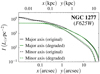 |
Fig. A.1. Major- (continuous line and coordinate x) and minor-axis (dashed line and coordinate y) surface brightness profiles of NGC 1277. Black lines come from our original MGE parametrisation (Fig. 10 and Sect. 3.2) and green ones were obtained from HST data that were degraded to a resolution corresponding to that of a galaxy at z = 1.2 as seen by the JWST. |
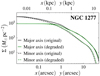 |
Fig. A.2. As Fig. A.1, but for the surface density profiles. As in Fig. 11, a Salpeter IMF was assumed. |
We produced Jeans models of NGC 1277 as in Sect. 4, but this time using the MGEs obtained from degraded data. Since we want to determine the black hole mass, we did a fit akin cC in Table 3, that is with a free MBH, a cylindrical velocity ellipsoid, and no variation in βz with radius. We call this model cCd (‘d’ stands for degraded). The fit is shown in Fig. A.3 and the fitted parameters are listed in Table A.3.
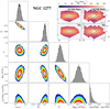 |
Fig. A.3. Same as Fig. 13, but this time we also fitted MBH and we used MGE parametrisations obtained from degraded HST images so to simulate how NGC 1277 would look like at z = 1.2 (fit cCd). |
JAM model fit parameters for NGC 1277 with the MGE parametrisation obtained from degraded HST data simulating JWST observations of a galaxy at a redshift z = 1.2.
Once again, we find a negligible dark matter fraction within 6 kpc. Perhaps the most surprising result is the detection of an extremely massive black hole, with MBH = (1.01 ± 0.10)×1010 M⊙. This mass is about two times larger than that found in Sect. 4.1. The mismatch parameter that we find here, α ≈ 1.5, is also significantly larger than in Sect. 4.1 (α ≈ 1.3).
Why is the black hole mass so large when using low angular resolution data? Accounting for the mismatch parameter, the stellar mass within the central kpc of NGC 1277 is M⋆(1 kpc) = 5.5 × 10¹⁰ M⊙ for the original MGE parametrisation. But this goes down to only M⋆(1 kpc) = 4.6 × 10¹⁰ M⊙ when using the degraded data. The central Vrms peak is the consequence of both a black hole and a peaked stellar distribution. If the peak in the stellar distribution is smoothened or erased, the algorithm assigns a larger mass to the black hole to compensate for the loss of the stellar cusp. Hence, our simple test tentatively indicates that black hole mass estimates obtained from insufficiently sharp data might be biased towards high values. It is noteworthy that in spite of the likely bias, we recover a black hole mass that is only a factor of roughly two off the one obtained using high-angular-resolution data.
Our test underlines the importance of properly characterising the central stellar distribution to be able to give an order-of-magnitude estimate of the mass of the central black hole. Using images with the JWST resolution concomitantly with a deconvolution method such as the Lucy-Richardson algorithm (Richardson 1972; Lucy 1974) it should be possible to recover information about the central stellar peak. Hence, such techniques should allow obtaining reasonable black hole mass estimates for galaxies with a central velocity dispersion cusp. Before being applied, this possibility hinted at by our relatively simple experiments should be confirmed with thorough tests made using mock simulated data.
All Tables
Parameters of the MGE decompositions of the surface brightness maps of NGC 1277 and NGC 1278.
Parameters of the MGE decompositions of the surface mass density maps of NGC 1277 and NGC 1278.
Parameters of the MGE decompositions of the degraded surface brightness map of NGC 1277.
Parameters of the MGE decompositions of the degraded surface mass density map of NGC 1277.
JAM model fit parameters for NGC 1277 with the MGE parametrisation obtained from degraded HST data simulating JWST observations of a galaxy at a redshift z = 1.2.
All Figures
|
Fig. 1. Map of the median intensity (left panel) and S/N per spectral pixel of 1.1 Å (right panel) in the wavelength range 4400 Å–6650 Å. The coordinates are centred in NGC 1277 and are in arcseconds. The black continuous shapes denote the effective radii of the galaxies as measured in Sect. 3.2. The effective radius of NGC 1277 has been de-circularised assuming an axial ratio |
| In the text | |
|
Fig. 2. Kinematic maps of NGC 1277. From left to right, V, σ, and Vrms maps of NGC 1277. The dashed line in the left panel indicates the kinematic major axis determined with kinemetry. The top row shows an interpolated version of the maps, whereas the lower one shows the individual fibre values. The grey contours denote isophotes separated by 0.5 mag arcsec−2 intervals obtained from an HST F625W image (top row) and from the integral field data integrated between 6150 Å and 6650 Å (lower row). The axes are in units of arcseconds. |
| In the text | |
|
Fig. 3. Same as Fig. 2, but for NGC 1278. In order to highlight the kinematic structures, the colour scales differ from those in Fig. 2. In this case, the top-row isophotes are based on an HST F850LP image, which is the one used for the MGE modelling detailed in Sect. 3.2. Since for this galaxy V ≪ σ, the Vrms map is virtually identical to the σ map. |
| In the text | |
|
Fig. 4. Relative difference between the 6150 Å−6650 Å normalised flux of the GCMS fibres and the flux from matched apertures of an HST F625W image smoothed to mimic the seeing of the ground-based observations. |
| In the text | |
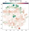 |
Fig. 5. Same as Fig. 4, but for NGC 1278 and a F850LP image. |
| In the text | |
|
Fig. 6. Position angle as a function of distance along the major axis for the ellipse fit of the HST imaging of NGC 1277 (left) and NGC 1278 (right). The error bars correspond to the one-sigma uncertainties. The vertical dashed lines indicate the radial interval over which the kinematical axis was determined. Its estimated value is indicated by the number in the lower part of the panels and the horizontal dotted lines. |
| In the text | |
|
Fig. 7. Velocity (top-row panels) and σ (lower-row panels) profiles for NGC 1277 (left-column panels) and NGC 1278 (right-column panels) as measured along the kinematic major axes. The black data points denote our measurements obtained from fibres whose centre is within the fibre radius ( |
| In the text | |
|
Fig. 8. Isophote plot derived from the HST F625W image of NGC 1277 with 0.5 mag arcsec−2 intervals (black contours). The corresponding MGE model isophotes are indicated in red. The blue ellipse denotes the extent of the region that was used to produce the MGE models (an ellipse with a semi-major axis of 32″, an ellipticity of 0.6, and a |
| In the text | |
|
Fig. 9. Same as Fig. 8, but for NGC 1278 and the HST F850LP image. The fitted area (blue circle) is 45″ in radius. |
| In the text | |
|
Fig. 10. Major- (continuous line and coordinate x) and minor-axis (dashed line and coordinate y) surface brightness profiles of NGC 1277 (left panel; in F625W) and NGC 1278 (right panel; in F850LP). Black lines come from our MGE fit and green ones come from Emsellem (2013) after a correction for extinction. The vertical grey lines indicate the maximum extent of the fitting area along the major (continuous) and the minor axis (dashed). For NGC 1278 the minor and major axis surface brightness profiles are nearly undistinguishable. The grey curves in the right panel correspond to the F625W surface brightness profiles calculated under the assumption that r − z = 0.74 (see text). |
| In the text | |
|
Fig. 11. Major- (continuous line and coordinate x) and minor-axis (dashed line and coordinate y) stellar surface density profiles of NGC 1277 (left panel) and NGC 1278 (right panel). The vertical grey lines are as in Fig. 10. The surface density estimates were calculated by deriving pixel-to-pixel mass-to-light ratios from colours following the prescriptions in Roediger & Courteau (2015), and assuming a Salpeter IMF. |
| In the text | |
|
Fig. 12. Dynamical modelling of the NIFS Vrms map of NGC 1277 assuming a cylindrically aligned velocity ellipsoid (fit cA1). The corner plot shows the probability distribution of the fitted parameters marginalised over either two parameters for the contour plots, and over one for the histograms. In the contour plots blue regions correspond to the three-sigma confidence level and white regions denote maximum likelihood. The top-right corner shows the Vrms map and the fit, with grey isophotes indicating F625W contours separated by 0.5 mag arcsec−2 and the black crosses indicating the centre of the bins. The indentations in the isophotes are a clear sign of the presence of the dust ring, whose near side was masked while producing the MGE models. The fitted parameters were q⋆ min, βz, α, and MBH, whereas the dark matter fraction fDM(6 kpc) was fixed to zero. |
| In the text | |
|
Fig. 13. As Fig. 12, but this time the fitted Vrms map is that of the GCMS data, fDM(6 kpc) (fDM(1.5 Re)) is a free parameter and the central black hole mass is fixed to MBH = 4.70 × 10⁹ M⊙ (fit cA2). As in Fig. 2, the Vrms maps are displayed in their interpolated (left) and individual-fibre (right) forms. They surface brightness contours correspond to HST data for the interpolated maps and to photometry derived from the CGMS data for the non-interpolated ones. |
| In the text | |
|
Fig. 14. Major- (blue) and minor-axis (red) Vrms profiles for the NIFS data of NGC 1277 (symbols) and the cA1 fit (continuous line). The error bars represent one-sigma Vrms formal uncertainties as obtained by pPXF (see Sect. 3.1). We selected the bins whose centres are within a cone with an aperture of 30° centred in the major (minor) axis. |
| In the text | |
|
Fig. 15. Same as Fig. 14, but this time for the GCMS data, the cA2 fit, and for fibres whose centre is within a fibre radius ( |
| In the text | |
|
Fig. 16. Same as Fig. 12, but this time for the GCMS Vrms map of NGC 1278 assuming a spherically aligned velocity ellipsoid (fit sB). The isophotes in the left-column maps come from an F850LP image. This is our fiducial fit for NGC 1278, where the fitted parameters are q⋆ min, βr, α, and MBH, and fDM(6 kpc) (fDM(1.5 Re)). |
| In the text | |
|
Fig. 17. Same as Fig. 14 but for NGC 1278 with GCMS data, and the SB fit. Because the galaxy is nearly spherical, we included data from all the fibres and sorted them according to their distance to the centre. |
| In the text | |
|
Fig. 18. Circularised mass-to-light ratio Υ⋆r as a function of the radius for NGC 1277 and NGC 1278, in blue and red respectively. The vertical lines indicate the limit of the GCMS kinematic data, The right axis shows the correspondence with the absolute value of the outer exponent of a bimodal IMF, Γb, for a stellar population with an age of 13.0 Gyr and a metallicity [Z/H] = 0.26. The horizontal black dashed lines denote the range of Γb values found by Martín-Navarro et al. (2015) for NGC 1277, with the upper line (Γb = 3.25) corresponding to their upper limit for the inner parts of the galaxy and the lower line (Γb = 2.15) corresponding to their lower limit at a radius R = 1.4 Re. The surface brightness of NGC 1278 has been converted to F625W as in Sect. 3.2. The correspondence between Υ⋆r and Γb is only roughly valid for NGC 1277 because NGC 1278 is slightly younger and less metallic (Ferré-Mateu et al., in prep.). |
| In the text | |
|
Fig. 19. Three-dimensional cumulative mass profiles of NGC 1277 for the baryonic component (stars plus black hole, in purple), the fitted dark matter halo (in black), and the predicted dark matter halo profiles for two different freezing redshifts (in blue and red for low and high zf, respectively) based on the SMHR parametrisation by Girelli et al. (2020) and the dark matter halo parametrisation by Child et al. (2018). The bands correspond to 95.4% confidence intervals. The baryonic component can be further subdivided into the black hole (dotted purple line) and the stellar component (dashed purple line). The grey vertical line indicates r = 6 kpc (18″), that is the radius within which we have kinematic data. |
| In the text | |
|
Fig. 20. Same as Fig. 19, but for NGC 1278. The dashed grey line indicates the radius out to which we have kinematic data, that is 10 kpc or 30″. |
| In the text | |
|
Fig. 21. Dark matter fraction within the effective radius, fDM(Re), as a function of the stellar mass for NGC 1277 and NGC 1278 (star symbols). The error bars represent one sigma confidence intervals (that corresponding to NGC 1277 is smaller than the symbol size). Circles correspond to the 103 ATLAS3D galaxies with good fits in Cappellari et al. (2013a) and the diamond symbols correspond to the data for a sample of 161 passive galaxies from the SAMI Galaxy Survey from Santucci et al. (2022). The colour coding of the symbols indicates the effective radius of the galaxies as shown by the side-bar. The ATLAS3D data points were derived by merging the galaxy distances from Cappellari et al. (2011), the effective radii and luminosities from Cappellari et al. (2013a), and the fDM(Re) and Υ⋆ values from Cappellari et al. (2013b). The effective radii for the SAMI galaxies were kindly provided by G. Santucci. The green line indicates the M⋆ − fDM(Re) relation derived from JAM models with a fixed cosmologically motivated NFW dark matter halo from Cappellari et al. (2013a). The red line and confidence band correspond to the fit represented in Fig. 7 from Santucci et al. (2022). The black line shows a prediction of the M⋆ − fDM(Re) relation made by combining the dark matter haloes derived from the SHMR from Girelli et al. (2020) and the dark matter halo parametrisation from Child et al. (2018) with the Re values derived from a linear fit (Eq. (20)) to the size measurements for galaxies with a morphological type T ≤ −1 in Trujillo et al. (2020). The latter relation was calculated assuming a de Vaucouleurs (1948) profile for the stellar component and it is complemented by a one-sigma uncertainty band calculated using a Montecarlo simulation. For the Trujillo et al. (2020) and the Santucci et al. (2022) data and the Girelli et al. (2020) SHMR, the stellar masses were corrected by a factor 0.23 dex to convert the assumed Chabrier (2003) IMF into a Salpeter (1955) one (see Eq. (3) in Sect. 3.2). |
| In the text | |
|
Fig. 22. Dark matter fraction within five effective radii fDM(5 Re) for NGC 1277 (star) with the 95.4% confidence interval indicated by a vertical line. The black line indicates the predicted M⋆ − fDM(5 Re) relation based on the dark matter haloes profiles and Re values derived as in Fig. 21. The grey shades indicate the 68.3% (darker) and 95.4% (lighter) confidence intervals of the relation calculated using a Montecarlo simulation. A de Vaucouleurs (1948) profile was assumed for the stellar density profile of the galaxies. |
| In the text | |
|
Fig. 23. Same as Fig. 22, but this time for the dark matter fraction enclosed within 6 kpc, fDM(6 kpc), and including the data point corresponding to NGC 1278. |
| In the text | |
|
Fig. A.1. Major- (continuous line and coordinate x) and minor-axis (dashed line and coordinate y) surface brightness profiles of NGC 1277. Black lines come from our original MGE parametrisation (Fig. 10 and Sect. 3.2) and green ones were obtained from HST data that were degraded to a resolution corresponding to that of a galaxy at z = 1.2 as seen by the JWST. |
| In the text | |
|
Fig. A.2. As Fig. A.1, but for the surface density profiles. As in Fig. 11, a Salpeter IMF was assumed. |
| In the text | |
|
Fig. A.3. Same as Fig. 13, but this time we also fitted MBH and we used MGE parametrisations obtained from degraded HST images so to simulate how NGC 1277 would look like at z = 1.2 (fit cCd). |
| In the text | |
Current usage metrics show cumulative count of Article Views (full-text article views including HTML views, PDF and ePub downloads, according to the available data) and Abstracts Views on Vision4Press platform.
Data correspond to usage on the plateform after 2015. The current usage metrics is available 48-96 hours after online publication and is updated daily on week days.
Initial download of the metrics may take a while.