| Issue |
A&A
Volume 658, February 2022
|
|
|---|---|---|
| Article Number | A76 | |
| Number of page(s) | 19 | |
| Section | Extragalactic astronomy | |
| DOI | https://doi.org/10.1051/0004-6361/202141762 | |
| Published online | 03 February 2022 | |
The MUSE Extremely Deep Field: Evidence for SFR-induced cores in dark-matter dominated galaxies at z ≃ 11
1
Univ. Lyon, Univ. Lyon1, Ens de Lyon, CNRS, Centre de Recherche Astrophysique de Lyon (CRAL) UMR5574, 69230 Saint-Genis-Laval, France
e-mail: This email address is being protected from spambots. You need JavaScript enabled to view it.
2
Leibniz-Institut für Astrophysik Potsdam (AIP), An der Sternwarte 16, 14482 Potsdam, Germany
3
European Southern Observatory (ESO), Karl-Schwarzschild-Strasse 2, 85748 Garching b. München, Germany
4
Institut de Recherche en Astrophysique et Planétologie (IRAP), Université de Toulouse, CNRS, UPS, 31400 Toulouse, France
5
Leiden Observatory, Leiden University, PO Box 9513 2300 RA Leiden, The Netherlands
6
Aix Marseille Univ., CNRS, CNES, LAM, Marseille, France
7
Instituto de Astrofísica e Ciências do Espaço, Universidade do Porto, CAUP, Rua das Estrelas, 4150-762 Porto, Portugal
8
Max Planck Institute for Astronomy, Königstuhl 17, 69117 Heidelberg, Germany
Received:
9
July
2021
Accepted:
23
October
2021
Abstract
Context. Disc-halo decompositions z = 1 − 2 star-forming galaxies (SFGs) at z > 1 are often limited to massive galaxies (M⋆ > 1010 M⊙) and rely on either deep integral field spectroscopy data or stacking analyses.
Aims. We present a study of the dark-matter (DM) content of nine z ≈ 1 SFGs selected among the brightest [O II] emitters in the deepest Multi-Unit Spectrograph Explorer (MUSE) field to date, namely the 140 h MUSE Extremely Deep Field. These SFGs have low stellar masses, ranging from 108.5 to 1010.5 M⊙.
Methods. We analyzed the kinematics with a 3D modeling approach, which allowed us to measure individual rotation curves to ≈3 times the half-light radius Re. We performed disk-halo decompositions on their [O II] emission line with a 3D parametric model. The disk-halo decomposition includes a stellar, DM, gas, and occasionally a bulge component. The DM component primarily uses the generalized α, β, γ profile or a Navarro-Frenk-White profile.
Results. The disk stellar masses M⋆ obtained from the [O II] disk-halo decomposition agree with the values inferred from the spectral energy distributions. While the rotation curves show diverse shapes, ranging from rising to declining at large radii, the DM fractions within the half-light radius fDM(< Re) are found to be 60% to 95%, extending to lower masses (densities) recent results who found low DM fractions in SFGs with M⋆ > 1010 M⊙. The DM halos show constant surface densities of ∼100 M⊙ pc−2. For isolated galaxies, half of the sample shows a strong preference for cored over cuspy DM profiles. The presence of DM cores appears to be related to galaxies with low stellar-to-halo mass ratio, log M⋆/Mvir ≈ −2.5. In addition, the cuspiness of the DM profiles is found to be a strong function of the recent star-formation activity.
Conclusions. We measured the properties of DM halos on scales from 1 to 15 kpc, put constraints on the z > 0 cvir − Mvir scaling relation, and unveiled the cored nature of DM halos in some z ≃ 1 SFGs. These results support feedback-induced core formation in the cold dark matter context.
Key words: galaxies: high-redshift / galaxies: evolution / galaxies: formation / galaxies: kinematics and dynamics / methods: data analysis
Based on observations made with ESO telescopes at the La Silla Paranal Observatory under the large program 1101.A-0127.
© N. F. Bouché et al. 2022
 Open Access article, published by EDP Sciences, under the terms of the Creative Commons Attribution License (https://creativecommons.org/licenses/by/4.0), which permits unrestricted use, distribution, and reproduction in any medium, provided the original work is properly cited.
1. Introduction
The universe’s matter content is dominated by elusive dark matter (DM), which has been one of the main topics in astronomical research. The idea of a dark or invisible mass was proposed numerous times based on the motions of stars in the Milky Way disk (Oort 1932), the motion of galaxies in the Coma cluster (Zwicky 1933), and by the lesser known argument made by Peebles & Partridge (1967) using an upper limit on the mean mass density of galaxies from the average spectrum of galaxies (i.e., from the night-sky brightness). Nonetheless, the concept of DM became part of mainstream research only in the 1970s, based on the remarkable fact that the rotation curves (RC) of massive galaxies remain flat at large galactocentric distances (Rubin & Ford 1970). It was quickly realized that these flat rotation curves at large radii could not be explained by the Newtonian gravity of the visible matter alone, but instead implied the presence of an unobserved mass component attributed to a DM halo.
Today, the cold-DM (CDM) framework in which the large-scale structure originates from the growth of the initial density fluctuations (Peebles & Yu 1970; Peebles 1974) is very successful in reproducing the large-scale structure (e.g., Springel et al. 2006). However, understanding the nature and properties of DM on galactic scales remains one of the greatest challenges of modern physics and cosmology (see Bullock & Boylan-Kolchin 2017, for a review).
In this context, disentangling and understanding the relative distributions of baryons and dark matter in galaxies is still best achieved from a careful analysis of galaxies’ RCs on galactic scales. At redshift z = 0, this type of analysis is mature with a wealth of studies published in the past 20−30 years, using a variety of dynamics tracers such as H I (e.g. de Blok & McGaugh 1997; de Blok et al. 2001; van den Bosch et al. 2000), Hα in the GHASP survey (Spano et al. 2008; Korsaga et al. 2018, 2019) or a combination of H I and Hα as in the recent SPARC sample (Allaert et al. 2017; Katz et al. 2017; Li et al. 2020) and the DiskMass survey (Bershady et al. 2010; Martinsson et al. 2013a). These studies have shown that, in low surface brightness (LSB) galaxies, the DM profiles have a flat density inner “core”, contrary to the expectations from DM-only simulations that DM haloes ought to have a steep central density profiles or “cusp” (e.g. Navarro et al. 1997, Navarro-Frenk-White: NFW). This cusp-core debate may be resolved within CDM with feedback processes (e.g. Navarro et al. 1996; Pontzen & Governato 2012; Teyssier et al. 2013; Di Cintio et al. 2014; Lazar et al. 2020; Freundlich et al. 2020a) transforming cusps into cores1, a process that could be already present at z = 1 (Tollet et al. 2016). DM-only simulations in the ΛCDM context have made clear predictions for the properties of DM halos, such as their concentration and evolution (e.g. Bullock et al. 2001; Eke et al. 2001; Wechsler et al. 2002; Duffy et al. 2008; Ludlow et al. 2014; Dutton & Macciò 2014; Correa et al. 2015), but the c − M relation remains untested beyond the local universe in SFGs (e.g. Allaert et al. 2017; Katz et al. 2017).
At high redshifts, where 21 cm observations are not yet available, in order to measure the DM content of high-redshift galaxies, one must measure the kinematics in the outskirts of individual star-forming galaxies (SFGs) using nebular lines (e.g. Hα), at radii up to 10−15 kpc (2−3 times the half-light radius Re) where the signal-to-noise ratio (S/N) per spaxel drops approximately exponentially and quickly falls below unity. Disk-halo decompositions have proven to be possible at z ≃ 2 in the pioneering work of Genzel et al. (2017) using very deep (> 30 h) near-IR integral field spectroscopy (IFS) on a small sample of six massive star-forming galaxies (SFGs). Exploring lower mass SFGs, this exercise requires a stacking approach (as in Lang et al. 2017; Tiley et al. 2019) or deep IFS observations (as in Genzel et al. 2020). These studies of massive SFGs with M⋆ > 1011 M⊙ showed that RCs are declining at large radii, indicative of a low DM fraction within Re; see also Wuyts et al. (2016), Übler et al. (2017), Abril-Melgarejo et al. (2021) for dynamical estimates of DM fractions.
Recently, 3D algorithms such as GALPAK3D (Bouché et al. 2015a) or 3DBAROLO (Di Teodoro & Fraternali 2015) have pushed the limits of what can be achieved at high-redshifts. For instance, one can study the kinematics of low mass SFGs, down to 108 M⊙ (as in Bouché et al. 2021) in the regime of low S/Ns or study the kinematics of SFGs at large galactic radii ∼3 × Re as in Sharma et al. (2021), when combined with stacking techniques. Most relevant for this paper, disk-halo decompositions of distant galaxies have been performed with 3DBAROLO at z ≃ 4 on bright submm [CII] ALMA sources (Rizzo et al. 2020; Neeleman et al. 2020; Fraternali et al. 2021). In addition, when used in combination with stacking or lensing, 3D algorithms are powerful tools to extract resolved kinematics at very high-redshifts as in Rizzo et al. (2021).
This paper aims to show that a disk-halo decomposition can be achieved for individual low-mass SFGs at intermediate redshifts (0.6 < z < 1.1) using the GALPAK3D algorithm combined with the deepest (140 h) Multi-Unit Spectroscopic Explorer (MUSE; Bacon et al. 2010) data obtained on the Hubble Ultra Deep Field (HUDF) and presented in Bacon et al. (2021). We show that rotation curves can be constrained up to 3 Re thanks to the 3D modeling approach on these deep IFU data. This paper is organized as follows. In Sect. 2, we present the sample used here. In Sect. 3, we present our methodology. In Sect. 4, we present our results. Finally, we present our conclusions in Sect. 6.
Throughout this paper, we use a ‘Planck 2015’ cosmology (Planck Collaboration XIII 2016) with ΩM = 0.307, Λ = 0.693, H0 = 67.7 km s−1 Mpc−1, yielding 8.23 physical kpc arcsec−1 at z = 1, and Δvir = 157.2. We also consistently use ‘log’ for the base-10 logarithm.
2. Sample
In this paper, we selected nine [O II] emitters from the recent MUSE eXtremely Deep Field (MXDF) region of the HUDF. The MXDF consists of a single MUSE field observed within the MUSE observations of the HUDF (Bacon et al. 2017) taken in 2018-2019 (PI. R. Bacon; 1101.A-0127) with the dedicated VLT GALACSI/Ground-Layer Adaptive Optics (AO) facility for a total of 140 h of integration. The MXDF field is thus located within the 9 sq. arcmin mosaic observations (at 10 h depth) and overlaps with the deep 30 h ‘UDF-10’ region, as described in Bacon et al. (2021) (their Fig. 1). The MXDF was observed with a series of 25 min exposures, each rotated by a few degrees yielding a final field of view that is approximately circular with radius 41″, where the deepest 140 h are contained within the central 31″ (see Bacon et al. 2021, for details). Thanks to the AO, the resulting point-spread function (PSF) full-width-at-half-max (FWHM) ranges from ≈0.6″ at 5000 Å to 0.4″ at 9000 Å.
The sample of [O II] emitters was selected from the mosaic catalogue (Inami et al. 2017) where we chose galaxies with the highest S/N per spaxel in [O II] that were not face-on (using the [O II] inclinations estimated in Bouché et al. 2021). From the catalog, we found 9 galaxies matching these criteria, listed in Table 1, with some reaching S/Npix ∼ 100 in the central spaxel. All galaxies but one are contained within the deepest 140 h MXDF circle of 31″. One galaxy, ID3, has only 24 h of integration in the MXDF dataset, but is fortuitously located in a deep stripe of the UDF10 region (Bacon et al. 2017) leading to a total of 42 h integration.
Properties of the SFGss selected in the MXDF.
These galaxies have redshifts ranging from 0.6 to 1.1, and have stellar masses from M⋆ = 108.9 M⊙ to M⋆ = 1010.3 M⊙ with SFRs from 1 to 5 M⊙ yr−1. The stellar masses and SFR were determined from spectral energy distribution (SED) fits with the MAGPHYS (da Cunha et al. 2015) software on the HST photometry (as in Maseda et al. 2017; Bacon et al. 2017, 2021) using a Chabrier (2003) initial mass function (IMF). Uncertainties on these quantities are obtained from the marginalized posterior probability distributions given by Magphys under the assumption of smooth star formation histories with additional random bursts (da Cunha et al. 2008, and references therein). The main properties of these galaxies are listed in Table 1.
In Fig. 1, we show the HST/F160W images of the nine SFGs where the background and foreground objects have been masked. This figure shows that not all galaxies are regular and axisymmetric. In particular, ID943 has a large companion 1″ away (masked) and ID919 has a small satellite at the same redshift, as seen in Fig. 2, and both of these galaxies show signs of tidal tails. ID3 has also a companion  away (masked).
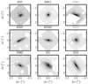 |
Fig. 1. Stellar continuum postage stamps. HST/F160W flux map for the nine [O II] emitters from the MXDF used in this study (ordered by increasing M⋆ from top left to bottom right). Background and foreground objects have been masked. The ellipse shows a constant isophote on the models. |
Using Sérsic (1963) fits with the GALF IT tool (Peng et al. 2002) on the HST/F160W WFC3 images, we find that these galaxies have surface brightness profiles consistent with an exponential. More specifically, we modeled the flux distribution using a single Sérsic profile with its total magnitude, effective radius, Sérsic index n, position angle (PA) and axis ratio (b/a) as free parameters, in combination with a sky component to take into account the sky background in the HST images. We used the F160W WFC3 images since these probe older stellar populations which better trace the underlying mass distribution and also because they have the best spatial resolution available. In order to improve the fits, we additionally masked the nearby objects appearing in the HST segmentation maps.
In order to get a measure of the galaxies bulge to total ratio (B/T), we remodeled them performing a multicomponent decomposition. This time, we used a combination of an exponential disk (with fixed n = 1) with a de Vaucouleurs bulge (with fixed n = 4, PA and b/a) on the same masked HST images.
3. Methodology
In order to measure the DM content of high-redshift galaxies, one must measure individual RCs in the outskirts of individual SFGs, at radii up to 10−15 kpc (2−3 Re) where the S/N per spaxel falls below unity. This is possible thanks to the combination of the deep MUSE data and 3D analysis tools such as GALPAK3D (Bouché et al. 2015a). In Sect. 3.1, we describe the 3D algorithm and our parameterization designed to analyze the shape of the RCs in order to characterize the outer slope of RCs. In Sect. 3.2, we describe our methodology for performing a full disk-halo decomposition directly to the 3D MUSE data-cubes.
3.1. Simultaneous measurements of the morphology and kinematics from 3D modeling
The GALPAK3D algorithm (Bouché et al. 2015a) compares 3D parametric models directly to the 3D data, taking into account the instrumental resolution and PSF2. Briefly, GALPAK3D performs a parametric fit of the 3D emission line data, simultaneously fitting the morphology and kinematics using a 3D (x, y, λ) disk model, which specifies the morphology and kinematic parametric profiles. GALPAK3D convolves the 3D model with the Point Spread Function and Line Spread Function, which implies that all the fitted parameters are “intrinsic” (i.e., corrected for beam smearing and instrumental effects).
For the morphology, the model assumes a Sérsic (1963) surface brightness profile Σ(r), with Sérsic index n. The disk model is inclined to any given inclination i and orientation or positional angle (PA). The thickness profile is taken to be Gaussian whose scale height hz is 0.15 × Re. For [O II] emitters, as in this analysis, we add a global [O II] doublet ratio rO2.
For the kinematics, the 3D model uses a parametric form for the rotation curve v(r) and the dispersion σ(r) profile as discussed in Bouché et al. (2021). In order to assess the shape of the RCs, we can use several RC models which allow for a rising or declining RC, such as in Rix et al. (1997), Courteau (1997) or the universal RC (URC) of Persic et al. (1996, PSS96). After experimentation, the latter is often our preferred choice because it has fewer parameter degeneracies. The URC of PSS96 has three parameters, the core radius rt, the velocity V2 (at Ropt ≃ 2Re) and the outer slope β of v(r).
Finally, as described in Bouché et al. (2015a, 2021), the velocity dispersion profile σt(r) consists of the combination of a thick disk σthick, defined from the identity σthick(r)/v(r) = hz/r (Genzel et al. 2006; Cresci et al. 2009) where hz is the disk thickness (taken to be 0.15 × Re) and a dispersion floor, σ0, added in quadrature (similar to σ0 in Genzel et al. 2006, 2008; Förster Schreiber et al. 2006, 2018; Cresci et al. 2009; Wisnioski et al. 2015; Übler et al. 2019).
Altogether, this 3D model (hereafter ‘URC’ model) has 13 parameters: xc, yc, zc, fO2, Re|O2, nO2, iO2, PA|O2, rt, V2, β, σ0 and the [O II] doublet ratio rO2. We use flat priors on these parameters and fit them simultaneously with a Bayesian Monte-Carlo algorithm. GALPAK3D can use a variety of Monte-Carlo algorithms and here we use the python version of MULTINEST (Feroz et al. 2009) from Buchner et al. (2014) because it is found to be very robust and insensitive to initial parameters. Moreover, it also provides the model evidence 𝒵.
There are several advantages to note here. The 3D algorithm GALPAK3D allows to fit the kinematics and morphological parameters simultaneously and thus no prior information is required on the inclination3. The agreement between HST-based and MUSE-based inclinations is typically better than 7° (rms) for galaxies with 25 < i < 80 as demonstrated in Contini et al. (2016) and with mock data-cubes (Bouché et al. 2021) derived from the Illustris “NewGeneration 50 Mpc” (TNG50) simulations (Nelson et al. 2019; Pillepich et al. 2019). Nonetheless, we checked that the inclinations i and Sérsic n parameters obtained from the [O II] MUSE data are consistent with those obtained from the HST/F160W images (see Tables 1 and 2). We find good agreement except for ID912 and ID919, which have the most face-on inclination with i⋆ < 30°. For these two galaxies, we restrict the GALPAK3D fits to iO2 < 35°.
Kinematics results from the GALPAK3D fits with our disk-halo decomposition.
3.2. Disk-halo decompositions
In most general terms, a disk-halo decomposition of the rotation curve v(r) is made of the combination of a dark-matter vdm, a stellar disk v⋆, a molecular vg, H2 and an atomic a gas vg,H I component:
 (1)
(1)
The mass profile for the molecular gas H2 component is negligible at low redshifts (due to the low gas fraction) (e.g. Frank et al. 2016). At high-redshifts, the molecular gas follows the SFR profile (or [O II]) (Leroy et al. 2008; Nelson et al. 2016; Wilman et al. 2020), and approximately the stellar component, and thus can become significant. However, because of the similar mass profile in molecular gas and stars, the two are inherently degenerate without direct CO measurements, currently inaccessible at our mass range. Depending on the molecular gas fractions, this component could be significant, but given that the molecular gas fractions in our redshift range 0.6 − 1.1 are typically 30−50% (e.g. Freundlich et al. 2019), this amounts to a systematic uncertainty of 0.1−0.15 dex on the mass of disk component.
The neutral gas profile vg,H I, however, is important given that (i), locally, it extends much further than the stellar component (e.g. Martinsson et al. 2013a; Wang et al. 2016, 2020) and can extend up to 40 kpc using stacking techniques (Ianjamasimanana et al. 2018), and (ii) at z ≈ 1 several absorption line surveys show extended cool structures that extend up to 80 kpc (e.g. Bouché et al. 2013, 2016; Ho et al. 2017, 2019; Zabl et al. 2019) traced by quasar Mg II absorption lines. Because of the roughly constant surface density of H I gas, this neutral gas contribution to v(r) is important at large distances (e.g. Allaert et al. 2017).
Within the context of this paper, we have implemented a 3D disk-halo decomposition in GALPAK3D, where the rotation curve is made of the combination of a dark-matter vdm, a disk v⋆, a neutral gas vg component (hereafter vg ≡ vg,H I):
 (2)
(2)
and in some cases an additional central or ‘bulge’ component vbg. For instance, ID982 has a B/T greater than 0.2 from the HST/F160W photometry (see Table 1). For these, we add a bulge to the flux profile and a Hernquist (1990) component vbg(r) to Eq. (2) whose parameters are the Sérsic index for the bulge nb (taken between nb = 2 and nb = 4), the bulge kinematic mass (vmax, b), the bulge radius rb and the bulge-to-total (BT) ratio.
The disk component v⋆ can be modeled as a Freeman (1970) disk suitable for exponential mass profiles and most of our galaxies have stellar Sérsic indices n⋆ close to n⋆ ≃ 1 (see Table 1). For a mass profile of any Sérsic n, the rotation curve v⋆(r) can be derived analytically (e.g. Lima Neto et al. 1999) or approximated using the Multi-Gaussian Expansion (MGE) approach of the spatial distribution (Emsellem et al. 1994a), assuming axisymmetry, with a sufficiently high number of gaussian components to ensure a given accuracy (e.g. < 1%) within 0.1 < r/Re < 20. Here, we use the MGE approach where the shape of v⋆(r) is determined by the Sérsic nO2 index from the [O II] SB profile, and the normalization of v⋆ is given by the disk mass M⋆, the sole free parameter. Naturally, this assumes that [O II] traces mass, which might not be appropriate. Hence, when preferred by the data (i.e., with a better evidence), we relax this constraint and use a Freeman (1970) disk (n ≡ 1) together with nO2 different than unity for the disk v⋆ component. For two galaxies, we selected this option (‘Freeman’ in Table 2).
The DM component vdm(r) can be modeled as a generalized α − β − γ double power-law model (Jaffe 1983; Hernquist 1990; Zhao 1996), hereafter the Hernquist-Zhao profile:
 (3)
(3)
where rs is the scale radius, ρs the scale density, and α, β, γ are the shape parameters, with β corresponding to the outer slope, γ the inner slope and α the transition sharpness.
The density ρs is set by the halo virial velocity Vvir (or halo mass Mvir), and following Di Cintio et al. (2014, hereafter DC14), rs can be scaled as
 (4)
(4)
where r−2 the radius at which the logarithmic DM slope is −24. The concentration cvir is defined as cvir, −2 ≡ Rvir/r−2, where Rvir is the halo virial radius (using the virial overdensity definition of Bryan & Norman 1998).
The shape parameters α, β, γ in Eq. (3) are a direct function of the disk-to-halo mass ratio log X ≡ log(M⋆/Mvir), in simulations with supernova feedback (e.g. DC14, Tollet et al. 2016; Lazar et al. 2020). This parameter X then uniquely determines the shape of the DM halo profile and its associated vdm(r). Hence, this DM profile vdm(r) has three free parameters, namely log X, Vvir and c−2. Since we used the α(X),β(X),γ(X) parametrisation with log X from DC14 (their Eq. (3)), we refer to this model as ‘DC14’, and refer the reader to DC14, Allaert et al. (2017), and Katz et al. (2017) for the details.
We also use a NFW DM profile, which is a special case of Hernquist-Zhao profiles with α, β, γ = (1, 3, 1)5. In Appendix C, we relax the DC14 assumption and explore Hernquist-Zhao DM profiles with unconstrained α, β, γ parameters (Fig. C.1), and refer this model as the ‘Zhao’ models. The shape of these DM profiles are not linked to log(M⋆/Mvir) as in DC14, and thus require a prior input for M⋆.
The gas component vg is made of a velocity profile  , appropriate for a gas distribution with a constant surface density Σg. This constant Σg is appropriate for H I gas profiles in the local universe (e.g. Martinsson et al. 2013a; Wang et al. 2016, 2020). Empirically, it has been shown that vg(r) can be well approximated with
  at z = 0 (e.g. Allaert et al. 2017). Here, Σg is an additional parameter which can be marginalized over. ΣHI is typically ∼5 M⊙ pc−2 (Martinsson et al. 2013a) which is a consistent with the well-known size-mass DH I − MH I z = 0 relation (Broeils & Rhee 1997; Wang et al. 2016; Martinsson et al. 2016; Lelli et al. 2016). We allowed ΣHI to range over 0 − 12.5 M⊙ pc−2. The maximum gas surface density at ∼10 M⊙ pc−2 can be thought as of a consequence of molecular gas formation (e.g. Schaye 2001).
Finally, we include the correction for pressure support (often called asymmetric drift correction) namely  following Weijmans et al. (2008), Burkert et al. (2010), and many others (see Appendix A), such that the circular velocity in Eq. (2) is
  where v⊥ is the observed rotation velocity. Since the ISM pressure P is approximately linearly dependent on the gas surface density Σg (e.g. Blitz & Rosolowsky 2006; Leroy et al. 2008), and can be described with
  (e.g Dalcanton & Stilp 2010), one has
 (5)
(5)
where rd is the disk scale length, (see Eq. (A.5)).
To summarize, the disk-halo 3D-model has 14 parameters: xc, yc, zc, fO2, Re, i, nO2, PA, Vvir, c−2, log X, σ0, Σg and the [O II] doublet ratio rO2. For the halo component, we can use a ‘DC14’ or an NFW model, for which, we use directly log M⋆ instead of log X as a parameter. For the ‘DC14’ halo model, we restrict log X to [−3.0, −1.2] to ensure a solution in the upper branch6 of the core-cusp vs. log X parameter space (see Fig. 1 of Di Cintio et al. 2014). In the cases with a bulge component, there are 4 additional parameters: rb, nb, vmax, b and B/T.
3.3. Parameter optimization and model selection
Having constructed disk-halo models in 3D(x, y, λ) within GALPAK3D, we optimize the 14 parameters simultaneously with GALPAK3D using the python PYMULTINEST package (Buchner et al. 2014) against the MUSE data where the stellar continuum was removed taking into account the PSF and LSF. As in Sect. 3.1, we use flat priors on each parameter. We also do not use the stellar mass from SED as input/prior on the disk mass (via log X) because the traditional disk-halo degeneracy is broken from the shape (α − β − γ) of the DM halo profile Eq. (3) which depends on the disk-to-halo mass ratio X = M⋆/Mvir as discussed in the previous section. We do not use priors on the inclination7 because the i − V degeneracy is broken from the simultaneous fit of the kinematics with the morphology, as discussed in Sect. 3.1.
Regarding model selection between DC14 or NFW DM profiles, we choose the preferred model by comparing the evidence ln𝒵 or marginal probability lnP(y|M1) (namely the integral of the posterior over the parameters space) (Jeffreys 1961; Kass & Raftery 1995; Robert et al. 2009; Jenkins & Peacock 2018) for the DC14 DM model (M1) against the NFW model (M2) and using the Bayes factor defined as the ratio of the marginal probabilities B12 ≡ P(y|M1)/P(y|M2). Throughout this paper, following Kass & Raftery (1995) (see also Gelman et al. 2014), we rescale the evidence by −2 such that it is on the same scale as the usual information criterion (Deviance, Bayesian Information Criterion, etc.). With this factor in mind, as discussed in Jeffreys (1961) and Kass & Raftery (1995), positive (strong) evidence against the null hypothesis (that the two models are equivalent) occurs when the Bayes factor is > 3 (> 20), respectively. This corresponds to a logarithmic difference Δln𝒵 of 2 and 6, respectively. Thus, we use a minimum Δln𝒵 of 6 as our threshold to discriminate between models. Table 3 shows the logarithmic difference of the Bayes factors, Δln𝒵, for the NFW DM models with respect to the fiducial DC14 models.
Bayesian evidences from the GALPAK3D fits.
3.4. Stellar rotation from HST photometry
In order to independently estimate the contribution of the stellar component to the RC, we parameterized the light distribution of HST/F160W images with the MGE method (Monnet et al. 1992; Emsellem et al. 1994b)8. For each galaxy we made an MGE model by considering the PSF of the HST/F160W filter, removing the sky level and masking any companion galaxies or stars. Each MGE model consists of a set of concentric 2D Gaussians defined by the peak intensity, the dispersion and the axial ratio or flattening. The Gaussian with the lowest flattening is critical as it sets the lower limit to the inclination at which the object can be projected (Monnet et al. 1992). Therefore, following the prescription from Scott et al. (2013), we also optimize the allowed range of axial ratios of all MGE models until the fits become unacceptable. In practice, convergence is achieved when the mean absolute deviation of the model for a given axial ratio pair increases by less than 10% over the previous step. Finally, we convert the Gaussian peak counts to surface brightness using the WFC3 zeropoints from the headers, and then to surface density (in L⊙ pc−2) adopting 4.60 for the absolute magnitude for the Sun in the F160W (Willmer 2018).
We follow the projection formulas in Monnet et al. (1992) and the steps outlined in Emsellem et al. (1994a,b) to determine the gravitational potential for our MGE models (see also Appendix A of Cappellari et al. 2002). The critical parameters here are the distance, inclination, and the mass-to-light ratio of the galaxy. The distances are simply calculated from the redshifts and our assumed Planck 2015 cosmology.
As we assume that the stellar component is distributed in a disk, we use the axial ratio of galaxies measured from the HST/F160W images to derive the inclinations of galaxies. An alternative approach would be to use the inclinations returned from the GALPAK3D models, which lead to almost identical results.
We estimate the mass-to-light ratios of galaxies combining the stellar masses obtained from photometric SED fits (see Sect. 2) and the total light obtained from the MGE models. Finally we use the module mge_vcirc from the JAM code (Cappellari 2008) to calculate the circular velocity in the equatorial plane of each galaxy.
4. Results
4.1. The diversity of rotation curve shapes
In Fig. 2, we show the morpho-kinematics of the galaxies used in this study. The first column shows the stellar continuum from HST/F160W. The second column shows the [O II] flux map obtained from the CAMEL9 algorithm (Epinat et al. 2012). The third column shows the [O II] surface brightness profile as a function of radius r, in units of Re. The fourth column shows the observed 2D velocity field v2d obtained from CAMEL. The fifth column shows the intrinsic rotation velocity v⊥(r) corrected for inclination and instrumental effects (beam smearing, see Sect. 3), using the parametric model of PSS96 (see Sect. 3.1). The vertical dotted lines represent the radius at which the S/N per spaxel reaches 0.3, and indicates the limits of our data. The last column shows the residual map, obtained from computing the standard deviation in the residual cube along the wavelength direction.
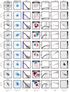 |
Fig. 2. Morpho-kinematics of each SFG. The columns shows (from left to right) the stellar continuum from HST/F160W, the [O II] flux map from MUSE, the [O II] surface brightness profile (SB(r)), the observed projected velocity field (v2d), the observed 1d velocity profile v⊥ sin i, the intrinsic (i.e., deprojected, corrected for beam smearing) modeled rotation curve (v⊥) using the URC model of PSS96 (see Sect. 3.1), and the residuals map obtained from the residual cube (see text). The red solid lines show the intrinsic SB(r) and v⊥ model. The solid black lines show the convolved SB profile and modeled 1d velocity profile. The gray symbols represent the data extracted from the flux and velocity maps. The blue vertical dotted lines represent 2 Re, while the red dotted lines show the radius at which the S/N per spaxel reaches 0.3. |
This figure shows that z = 1 RCs have diverse shapes (as in Tiley et al. 2019; Genzel et al. 2020) with mostly increasing but some presenting declining RCs at large radii as in Genzel et al. (2017). The diversity, albeit for a smaller sample, is similar to the diversity observed at z = 0 (e.g. Persic et al. 1996; Catinella et al. 2006; Martinsson et al. 2013b; Katz et al. 2017).
4.2. The disk-halo decomposition
We now turn to our disk-halo decomposition using the method described in Sect. 3.2. For each SFG, we ran several combinations of disk-halo models, such as different halo components (DC14/NFW), different disk components (Freeman/MGE), with or without a bulge, with various asymmetric drift corrections and chose the model that best fit the data for each galaxy according to the model evidence. We find that the DC14 halo model is generally preferred over a NFW profile and the resulting model parameters are listed in Table 2. The evidence for the DC14 models is discussed further in Sect. 4.6.
Before showing the disk-halo decompositions, we compare the disk stellar mass M⋆ (M⋆ being one of the 14 free parameters) obtained from the 3D fits with the SED-derived M⋆. This comparison is performed in Fig. 3 where the total M⋆ (disk+bulge from our fits) is plotted along the x-axis. This figure shows that there is relatively good agreement between the disk mass estimates from our GALPAK3D model fits (described in Sect. 3.2) and the SED-based ones, except for ID919 and ID943. This figure shows that our 3D disk-halo decomposition yields a disk mass consistent with the SED-derived M⋆, and thus opens the possibility to constrain disk stellar masses from rotation curves of distant galaxies for kinematically undisturbed galaxies.
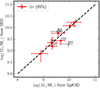 |
Fig. 3. Comparison of SED-based stellar masses and kinematic-based stellar masses. The kinematic-based stellar mass M⋆ are obtained from GALPAK3D disk-halo fits, while the SED-based M⋆ are derived from the HST photometry. The error bars represent the 95% confidence intervals. The M⋆ obtained with GALPAK3D (one of the 14 free parameters in Sect. 3.2) and from HST photometry are completely independent, except for ID912 (open circle). The dashed line shows the 1:1 line and this figure shows the two are in excellent agreement, except for ID919 and ID943. |
The disk-halo decompositions (deprojected and ‘deconvolved’ from instrumental effects) using our 3D-modeling approach with GALPAK3D are shown in Fig. 4, where the panels are ordered by increasing M⋆ as in Fig. 1. The disk/DM models used are listed in Table 2. In each panel, the solid black line shows the total rotation velocity v⊥(r) corrected for asymetric drift. All velocities are ‘intrinsic’, meaning corrected for inclination and instrumental effects, while the dot-dashed line represents the circular velocity vc(r). The gray band represents the URC model as in Fig. 2. The solid green, red and blue lines represent the dark-matter vdm(r), stellar v⋆(r), and gas components vg(r), respectively. The dotted red lines represent the stellar component obtained from the HST/F160W images as discussed in Sect. 3.4.
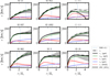 |
Fig. 4. Disk-halo decompositions for the nine galaxies in our sample (ordered by increasing M⋆). The solid black line represents the total rotation velocity v⊥(r). All velocities are ‘intrinsic’, that is corrected for inclination and instrumental effects. The dot-dashed line represents the circular velocity vc(r), that is v⊥(r) corrected for asymmetric drift. The gray band represents the intrinsic universal rotation curve (URC) using the parameterization of PSS96 as in Fig. 2. The solid red (blue) line represents the stellar (gas) component v⋆(r) obtained from GALPAK3D modeling of the MUSE [O II] data. The dotted red line represents the stellar component obtained using a MGE decomposition of the HST/F160W stellar continuum images. The green line represents the DM component. The vertical dotted lines are as in Fig. 2. |
Comparing the solid with the dotted red lines in Fig. 4, one can see that there is generally good agreement between v⋆(r) obtained from the HST photometry and from our disk-halo decomposition with GALPAK3D of the MUSE data, except again for ID919 and ID943. This comparison shows that the disk-halo decomposition obtained from the [O II] line agrees with the v⋆ from the mass profile obtained on the HST photometry. One should note that the stellar mass M⋆ from SED fitting is not used as a prior in our GALPAK3D fits, except for ID937 because the data for this galaxy prefers a NFW profile, which then becomes degenerate with M⋆. For the interested reader, the potential degeneracies between M⋆ and Mvir are shown in Fig. B.2.
4.3. The stellar-to-halo mass relation
The M⋆ − Mvir relation in ΛCDM is a well-known scaling relation that reflects the efficiency of feedback. Hence, measuring this scaling relation in individual galaxies is often seen as a crucial constraint on models for galaxy formation. This scaling relation can be constructed from abundance matching techniques (e.g. Vale & Ostriker 2004; Moster et al. 2010; Behroozi et al. 2013, 2019). Observationally, the z = 0 stellar-to-halo relation has been constrained by numerous authors using a variety of techniques such as weak lensing and/or clustering (e.g. Leauthaud et al. 2012; Mandelbaum et al. 2016). Direct measurements of the M⋆ − Mvir relation on individual galaxies using rotation curves have been made on various samples of dwarfs (Read et al. 2017), spirals (Allaert et al. 2017; Katz et al. 2017; Lapi et al. 2018; Posti et al. 2019; Di Paolo et al. 2019) and early type galaxies (Posti & Fall 2021) among the most recent studies, and these have found a very significant scatter in this relation.
In Fig. 5 (left), we show the stellar-to-halo mass ratio M⋆/Mvir as a function M⋆. The blue (gray) contours show the expectation for z = 1 SFGs in the TNG100/50 simulations and the solid lines represent the M⋆/Mvir relation from Behroozi et al. (2019). Figure 5 (left) shows that our results are qualitatively in good agreement with the Behroozi relation.
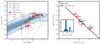 |
Fig. 5. Total stellar-to-halo fraction. Left: total stellar-to-halo fractions M⋆/Mvir as a function of the stellar mass M⋆ obtained from our 3D fits. The error bars from our data are 95% confidence intervals, and the open circles show the sample of Genzel et al. (2020). The shaded (blue contours) histogram shows the location of SFGs in the TNG simulations for z = 1 centrals, while the gray contours show the satellites. The colored lines show the Behroozi et al. (2019) relation inferred from semi-empirical modeling at redshifts z = 0.5, 1.0, 1.5, respectively. Right: total stellar-to-halo fractions M⋆/Mvir as a function of GMvir/j⋆σ⋆ (Eq. (7)) for the galaxies in our sample. The inset histogram shows that the sample has |
Romeo (2020) argued that disk gravitational instabilities are the primary driver for galaxy scaling relations. Using a disk-averaged version of the Toomre (1964)Q stability criterion10, Romeo (2020) find that
 (6)
(6)
where i = ⋆, H I or H2,  is the radially averaged velocity dispersion, and ji is the total specific angular-momentum. For i = ⋆, Ai ≈ 0.6.
Consequently, for the stellar-halo mass relation with i = ⋆, M⋆/Mvir ought to correlate with (Romeo et al. 2020):
 (7)
(7)
where j⋆ is the stellar specific angular momentum,  the radially averaged stellar dispersion. We can estimate j⋆ using the ionized gas kinematics, namely log j⋆ = log jgas − 0.25 as in Bouché et al. (2021). The dispersion
  is not directly accessible, but we use the scaling relation with M⋆ (
 ) from Romeo et al. (2020) which followed from the Leroy et al. (2008) analysis of local galaxies. Figure 5 (right) shows the resulting stellar-to-halo mass ratio using M⋆ from SED and the Mvir values obtained from our disk-halo decomposition, where the inset shows the sample has ⟨Q⋆⟩≈0.7, close to the expectation (Eq. (6)).
4.4. DM fractions in z = 1 SFGs
Using the disk-halo decomposition shown in Fig. 4, we turn toward the DM fraction within Re, fDM(< Re), by integrating the DM and disk mass profile to Re11. Figure 6 shows that fDM(< Re) for the galaxies in our sample is larger than 50% in all cases, ranging from 60% to 90%. The left (right) panel of Fig. 6 shows fDM(< Re) as a function of Mvir (Σ⋆, 1/2 the surface density within Re), respectively. Compared to the sample of 41 SFGs from Genzel et al. (2020) (open circles), our sample extends their results to the low mass regime, with M⋆ < 1010.5 M⊙, Mvir < 1012 M⊙ and to lower mass surface densities Σ⋆ < 108 M⊙ kpc−2.
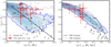 |
Fig. 6. DM fractions for our SFGs. Left: DM fractions within the half-light radius Re, fDM(< Re), as a function of halo mass, Mvir. The dashed line represent the downward trend of Genzel et al. (2020). Right: DM fractions within Re as a function of stellar mass surface density Σ⋆, 1/2 within Re. In both panels, the error bars from our data are 95% confidence intervals, and the open circles show the sample of Genzel et al. (2020). The shaded (blue contours) histogram shows the location of SFGs in the TNG100 simulations for z = 1 central SFGs, while the gray contours show the satellites. The dotted line represents the toy model derived from the TF relation (Eq. (9)). |
The relation between fDM and Σ⋆, 1/2 in Fig. 6 is tighter and follows the expectation for z = 1 SFGs in the TNG100/50 simulations (blue contour) (Lovell et al. 2018; Übler et al. 2021), except at high masses. Genzel et al. (2020) already noted that the correlation with Σ⋆ is better than with Vvir or Mvir. This anticorrelation between the baryonic surface density and DM fraction has been noted at z = 0 in several disk surveys (e.g. Bovy & Rix 2013; Courteau & Dutton 2015, see their Fig. 23).
In Sect. 5.1, we discuss the implications of this fDM − Σ⋆ relation and its relation to other scaling relations.
4.5. DM halo properties. The c−M scaling relation
Having shown (Figs. 3 and 4) that the baryonic component from our 3D fits is reliable, we now turn to the DM properties of the galaxies, and in particular to the concentration-halo mass relation (cvir − Mvir).
The c − M relation predicted from ΛCDM models (e.g. Bullock et al. 2001; Ludlow et al. 2014; Dutton & Macciò 2014; Correa et al. 2015) is often tested in the local universe (e.g. Allaert et al. 2017; Katz et al. 2017; Leier et al. 2012, 2016, 2022; Wasserman et al. 2018), but rarely beyond redshift z = 0 except perhaps in massive clusters (e.g. Buote et al. 2007; Ettori et al. 2010; Sereno et al. 2015; Amodeo et al. 2016; Biviano et al. 2017). These generally agree with the predicted mild anticorrelation between concentration and virial mass.
Figure 7 (left) shows the cvir − Mvir relation for the best 6 cases in our sample, that is excluding the two interacting galaxies (ID919, ID943) as well as ID15 because its concentration parameter remains unconstrained and degenerate with Vvir (see Fig. B.2b). The error bars represent 2σ (95%) and are color-coded according to the galaxy redshift. In Fig. 7 (left), the solid lines color coded with redshift represent to the c − M relation from Dutton & Macciò (2014).
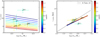 |
Fig. 7. Size of DM cores. Left: halo concentration-halo mass relation. The concentrations cvir for z ≃ 1 SFGs, derived from our 3D modeling of the [O II] rotation curves, are converted to a DM-only NFW equivalent cvir, DMO (see text). Right: DM core size rs, DMO ≡ Rvir/cvir, DMO in kpc as a function of halo mass. The dotted line represents the observed core-mass scaling relation for z = 0 LSBs from Di Paolo et al. (2019) (see text). In both panels, the solid lines represent the cvir − Mvir relation predicted by Dutton & Macciò (2014) for DM halos, color-coded by redshift. The error bars are 95% confidence intervals (2σ) and color-coded also by the galaxy redshift. |
We note that in order to fairly compare our data to such predictions from DM-only (DMO) simulations, we show, in Fig. 7, the halo concentration parameter cvir corrected to a DM-only (DMO) halo following DC1412:
![Mathematical equation: $$ \begin{aligned} c_{\rm vir,DMO} = \frac{c_{\rm vir,-2}}{1 + 0.00003 \times \exp [3.4 (\log X + 4.5)]}\cdot \end{aligned} $$](/articles/aa/full_html/2022/02/aa41762-21/aa41762-21-eq46.gif) (8)
(8)
We note that the correction is important only for halos with stellar-to-halo mass ratio log X > −1.5 and that most of our galaxies (7 out of 9) have log X < −1.5.
Figure 7 (right) shows the corresponding scaling relation for the scaling radius rs, namely the rs − Mvir relation. This relation in terms of rs is redshift independent. Several authors have shown, in various contexts (i.e., using pseudo-isothermal or Burkert 1995 profiles), that this quantity scales with galaxy mass or luminosity (e.g. Salucci et al. 2012; Kormendy & Freeman 2016; Di Paolo et al. 2019). For illustrative purposes, we show the recent z = 0 sequence for low surface brightness (LSB) galaxies of Di Paolo et al. (2019).
Figure 7 shows that 5 of the 6 SFGs tend to follow the expected scaling relations for DM, the exception being ID912. One should keep in mind that cosmological simulations predict a c − M relation with a significant scatter (e.g. Correa et al. 2015). To our knowledge, Fig. 7 is the first test of the c − M relation at z > 0 on halos with log Mvir/M⊙ = 11.5−12.5 and our data appears to support the expectations from ΛCDM.
The cvir − Mvir or rs − Mvir relations can be recasted as a rs − ρs relation (from Eq. (3)). Figure 8 (left) shows the ρs − rs relation and confirms the well-known anticorrelation between these two quantities with a slope of ≈ − 1 (e.g. Salucci & Burkert 2000; Kormendy & Freeman 2004, 2016; Martinsson et al. 2013b; Spano et al. 2008; Salucci et al. 2012; Ghari et al. 2019; Di Paolo et al. 2019; Li et al. 2019), which has been found in a wide range of galaxies (dwarfs disks, LSBs, spirals). These results are similar in nature, in spite of using different contexts and assumptions (namely ρ0 vs ρ−2 or ρs). A detailed investigation of the differences related to these assumptions is beyond the scope of this paper.
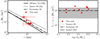 |
Fig. 8. Halo scale radius-density relation at z = 1. Left: ρs − rs scaling relation for the galaxies shown in Fig. 7. The error bars are 95% confidence intervals (2σ). For comparison, the anticorrelation of Kormendy & Freeman (2004), Spano et al. (2008) and Di Paolo et al. (2019) are shown. Right: DM surface density (Σs ≡ ρs rs) as a function of galaxy mass. The anticorrelation in the left panel implies a constant DM surface density. The gray band represents the range of surface densities from Burkert (2015) for dwarfs. The constant densities of Kormendy & Freeman (2004) and Donato et al. (2009) are shown as the dotted, dot-dashed lines, respectively. |
As discussed in Kormendy & Freeman (2004), this anticorrelation can be understood from the expected scaling relation of DM predicted by hierarchical clustering (Peebles 1974) under initial density fluctuations that follow the power law |δk|2 ∝ kn (Djorgovski 1992). Djorgovski (1992) showed that the size R, density ρ of DM halos should follow ρ ∝ R−3(3 + n)/(5 + n). For n ≃ − 2 on galactic scales, ρ ∝ R−1. This anticorrelation is also naturally present in the ΛCDM context as shown by Kravtsov et al. (1998) with numerical simulations. As noted by many since Kormendy & Freeman (2004), the anticorrelation between ρs and rs implies a constant DM surface density Σs ≡ ρs rs (e.g. Donato et al. 2009; Salucci et al. 2012; Burkert 2015; Kormendy & Freeman 2016; Karukes & Salucci 2017; Di Paolo et al. 2019). Figure 8 (right) shows the resulting DM surface density Σs as a function of galaxy mass Md. The gray band represents the range of surface densities from Burkert (2015) for dwarfs, while the dashed line represents the range of densities from Donato et al. (2009), Salucci et al. (2012) for disks. Kormendy & Freeman (2004) had found a value of ∼100 M⊙ pc−2.
4.6. DM halos properties with core or cuspy profiles
We now investigate the shape of DM profiles, and in particular the inner logarithmic slope γ (ρdm ∝ r−γ) in order to find evidence against or for core profiles. There is a long history of performing this type of analysis in local dwarfs (e.g. Kravtsov et al. 1998; de Blok et al. 2001; Goerdt et al. 2006; Oh et al. 2011, 2015; Read et al. 2016b, 2018, 2019; Karukes & Salucci 2017; Zoutendijk et al. 2021), in spiral galaxies (e.g. Gentile et al. 2004; Spano et al. 2008; Donato et al. 2009; Martinsson et al. 2013a; Allaert et al. 2017; Katz et al. 2017; Korsaga et al. 2018; Di Paolo et al. 2019) or in massive early type galaxies often aided by gravitational lensing (e.g. Suyu et al. 2010; Newman et al. 2013; Sonnenfeld et al. 2012, 2013, 2015; Oldham & Auger 2018; Wasserman et al. 2018), but the core/cusp nature of DM is rarely investigated in SFGs outside the local universe (except in Genzel et al. 2020; Rizzo et al. 2021) because this is a challenging task. However, owing to the high DM fractions in our sample (see Fig. 6), the shape the rotation curves are primarily driven by the DM profile.
The DM profiles ρdm(r) as a function of r/Re obtained from our 3D fits with the DC14 model are shown in Fig. 9. This figure shows that the NFW profile is not compatible with the majority of the SFGs. Figure 9 shows that at least three galaxies (IDs 37, 912, 982) show strong departures from a NFW profile, in particular they show evidence for cored DM profiles. For these three galaxies, the logarithmic difference of the Bayes factors for the NFW profiles are > 100 (see Table 3), indicating very strong evidence against cuspy NFW profiles. Our results are in good agreement with the RC41 sample of Genzel et al. (2020) where about half of their sample showed a preference for cored profiles (their Fig. 10).
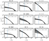 |
Fig. 9. DM density profiles in M⊙/kpc3. Each panel show ρdm(r) as a function of r/Re obtained from our disk-halo decompositions (Fig. 4). The stellar-to-halo-mass ratio (log X ≡ log M⋆/Mvir) is indicated. The gray bands represent the 95% confidence interval and the dotted lines represent NFW profiles. The vertical dotted lines represent the 1 kpc physical scale, corresponding to ≈1 MUSE spaxel, and indicates the lower limit of our constraints. |
Before discussing the implications of these results in Sect. 5.2, we show in Fig. 10 (left) the constraints on the DM shape parameters (α, β, γ) as a function of log X in the context of ‘DC14’ models, except for ID937 where we used a ‘NFW’ profile. The errorbars are 95% confidence intervals. For the curious reader, we show in Fig. C.1 (left) the constraints on these shape parameters when we relax the DC14 assumption, i.e. using Hernquist-Zhao DM profiles, and the SED stellar mass as prior.
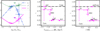 |
Fig. 10. Relation between SFR and cores. Left: α, β, γ parameters as a function of log M⋆/Mvir. The curves show the parameterisation of DC14 for α, β, γ and the solid symbols represent our SFGs, excluding ID919 and 943. Middle: DM inner slope γ as a function of the SFR surface density ΣSFR, scaled to z = 1.5. Right: DM inner slope γ as a function of the logarithmic offset from the MS, δ(MS), using the Boogaard et al. (2018) MS. DM cores are present in galaxies with higher SFR and SFR surface-densities. |
In a subsequent paper, we will analyze additional DM profiles for CDM (e.g. Einasto 1965; Burkert 1995; Dekel et al. 2017; Freundlich et al. 2020b) including alternative DM models such as “fuzzy” axion-like DM (Weinberg 1978; Burkert 2020), self-interacting DM (SIDM; Spergel & Steinhardt 2000; Vogelsberger & Zavala 2013).
5. Discussion
5.1. DM fractions in z = 1 SFGs
We return to the fDM − Σ⋆ relation in Fig. 6 and its implications. The tight fDM − Σ⋆ relation can be thought of as a consequence of the tight Tully & Fisher (1977) relation (TFR) for disks as follows (see also Übler et al. 2017). Indeed, if we approximate the DM fraction within Re as  (Genzel et al. 2020), one has
  . Thus,
 (9)
(9)
where we used the stellar TFR,  (e.g. McGaugh 2005), the definition of gas-to-stellar mass ratio μg ≡ Mgas/M⋆ and the maximum stellar rotation velocity for disks
  . Equation (9) shows the intimate link between the fDM − Σ⋆ diagram and the TFR relation.
More specifically, the TFR has  with n ≃ 4, a ≃ 1010 M⊙ (McGaugh 2005; Meyer et al. 2008; Cresci et al. 2009; Pelliccia et al. 2017; Tiley et al. 2016; Übler et al. 2017; Abril-Melgarejo et al. 2021) where Vrot, 2.2 ≡ Vrot/102.2 km s−1. Given that
  for a Freeman (1970) disk,
  becomes
 (10)
(10)
using Re = 1.68 Rd, where M⋆, a ≡ M⋆/a. For a z ≈ 1 TFR with n = 3.8 and a = 109.8 M⊙ (e.g. Übler et al. 2017), Eq. (9) results in  , which is shown in Fig. 6 (right) as the dotted line with fg = 0.5 (e.g. Tacconi et al. 2018; Freundlich et al. 2019). This exercise shows that the fDM − Σ⋆ relation is another manifestation of the TFR as argued in Übler et al. (2017).
5.2. Core/cusp formation
Our results in Sect. 4.6 (Fig. 9) indicate a strong preference for cored DM profiles for four SFGs in our sample. Several mechanisms have been invoked to explain the presence of cored DM profiles such as Warm Dark Matter (WDM, Bode et al. 2001), whose free streaming can suppress the small-scale fluctuations, axion-like “fuzzy” DM (Weinberg 1978; Hu et al. 2000; Burkert 2020), baryon-DM interactions (Famaey et al. 2018), SIDM (Spergel & Steinhardt 2000; Burkert 2000; Vogelsberger et al. 2013) or dynamical friction (Read et al. 2006; Goerdt et al. 2010; Orkney et al. 2021) from infalling satellites/minor mergers.
Within the context of CDM, it has long been recognized (see review in Bullock & Boylan-Kolchin 2017) since the original cusp/core problem first observed in dwarfs or low-surface brightness galaxies (e.g. de Blok & McGaugh 1997; de Blok et al. 2001; Kravtsov et al. 1998) that (rapid) changes in the gravitational potential due to star-formation driven outflows can essentially inject energy in the DM, resulting in a flattened DM profile (Navarro et al. 1996; Read & Gilmore 2005; Pontzen & Governato 2012; Teyssier et al. 2013; Di Cintio et al. 2014; Dutton et al. 2016, 2020; Chan et al. 2015; El-Zant et al. 2016; Lazar et al. 2020; Freundlich et al. 2020a). Similarly, DM core/cusps can also be linked to active galactic nuclei (AGN) activity (Peirani et al. 2017; Dekel et al. 2021) in more massive galaxies with Mvir > 1012 M⊙. While most of these analyses focus at cores at z = 0, Tollet et al. (2016) showed that cores can form in a similar fashion as early as z = 1.
Observationally, cores are now found up to z ≃ 2 (Genzel et al. 2020), but the relation between outflows/star-formation and core formation has not been established, as observations have unveiled cores in galaxies spaning a range of halo or stellar masses (e.g. Wasserman et al. 2018, and references therein) or cusps when cores would be expected (e.g Shi et al. 2021). At high-redshifts, Genzel et al. (2020) found that cores are preferentially associated with low DM fractions.
In order to investigate the potential relation between SFR-induced feedback and DM cores, we show in Fig. 10 the DM inner slope γ as a function of SFR surface density ΣSFR (middle) and as a function of the offset from the main-sequence (MS) for SFGs (using Boogaard et al. 2018) (right). This figure indicates that SFGs above the MS or with high-SFR densities are preferentially found to have cores. SFGs below the MS with decaying SFR (like ID15) have low SFR densities owing to the low SFR, and show cuspy DM profiles, indicating that cusps reform when galaxies stop being active.
While the majority of research has focused on the formation of DM cores in order to match observations at z = 0, DM cusps can reform from the accretion of DM substructures (Laporte & Peñarrubia 2015) as first argued in Dekel et al. (2003), or as a result of late mergers as argued in Orkney et al. (2021) for dwarfs.
In Fig. 11, we compare our results to those of Read et al. (2019) who found that dwarfs fall in two categories, where the core/cusp presence is related to the star-formation activity. Read et al. (2019) found that dwarfs whose star-formation stopped over 6 Gyr ago show preferentially cusps (open red squares), while dwarfs with extended star-formation show shallow DM cores (open blue squares). In this figure, the filled red (blue) circles represent our galaxies with ΣSFR smaller (larger) than log ΣSFR/M⊙ kpc−2 = −0.7. Our results in Fig. 11, together with those of Read et al. (2019), provide indirect evidence for SFR-induced core formation within the CDM scenario, where DM can be kinematically heated by SFR-related feedback processes.
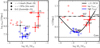 |
Fig. 11. Left: DM density at 150 pc as a function of log M⋆/Mvir. The blue (red) solid circles with error bars (2σ) show our SFGs, except ID919 and 943. Right: DM inner slope γ parameter at 150 pc as a function of log M⋆/Mvir. The blue (red) squares represent the z ≈ 0 dwarfs from Read et al. (2019) whose SFR was truncated less (more) than 6 Gyr ago. The blue (red) solid circles with error bars (2σ) show our SFGs with high (low) ΣSFR, respectively. |
6. Conclusions
Using a sample of nine [O II] emitters with the highest S/Ns in the deep (140 h) MXDF (Bacon et al. 2021) dataset, we measure the shape of individual RCs of z ≈ 1 SFG out to 3 × Re with stellar masses ranging from 108.5 to 1010.5 M⊙, covering a range of stellar masses complementary to the analysis of Genzel et al. (2020), whose sample has M⋆ > 1010 M⊙.
We then performed a disk-halo decomposition on the [O II] emission lines using a 3D modeling approach that includes stellar, dark-matter, gas (and bulge) components (Fig. 4). The dark-matter profile is a generalized Zhao (1996) profile using the feedback prescription of Di Cintio et al. (2014), which links the DM profile shape to the baryonic content.
Our results are as follows. We find that:
– The 3D approach allows to constrain RCs to 3Re in individual SFGs revealing a diversity in shapes (Fig. 2) with mostly rising and some having declining outer profiles;
– The disk stellar mass M⋆ from the [O II] rotation curves is consistent with the SED-derived M⋆ (Fig. 3), except for two SFGs (IDs 919, 943) whose kinematics are strongly perturbed by a nearby companion (< 2″);
– The stellar-to-DM ratio M⋆/Mvir follows the relation inferred from abundance matching (e.g. Behroozi et al. 2019), albeit with some scatter (Fig. 5);
– The DM fractions fDM(< Re) are high (60−90%) for our nine SFGs (Fig. 6) which have stellar masses (from 108.5 M⊙ to 1010.5 M⊙) or surface densities (Σ⋆ < 108 M⊙ kpc−2). These DM fractions complement the low fractions of the sample of Genzel et al. (2020), and globally, the fDM(< Re)−Σ⋆ relation is similar to the z = 0 relation (e.g. Courteau & Dutton 2015), and follows from the TFR;
– The fitted concentrations are consistent with the cvir − Mvir scaling relation predicted by DM only simulations (Fig. 7);
– The DM profiles show constant surface densities at ∼100 M⊙ pc−2 (Fig. 8);
– Similarly to the z > 1 samples of Genzel et al. (2020), the disk-halo decomposition of our z ≈ 1 SFGs shows cored DM profiles for about half of the isolated galaxies (Figs. 9 and 10) in agreement with other z = 0 studies (e.g. Allaert et al. 2017; Katz et al. 2017);
– DM cores are present in galaxies with high SFRs (above the MS), or high SFR surface density (Figs. 10b and c), possibly supporting the scenario of SN feedback-induced core formation. Galaxies below the MS or low SFR surface density have cuspy DM profiles (Fig. 11), suggesting that cusps can reform when galaxies become passive (e.g. Laporte & Peñarrubia 2015; Chan et al. 2015; Orkney et al. 2021).
Overall, our results demonstrate the power of performing disk-halo decomposition in 3D on deep IFU data. With larger samples, it should be possible to confirm this type of relation between cores and star-formation histories, and to test further SN feedback induced core formation within the ΛCDM framework.
Recently, Pineda et al. (2017) argued that NFW profiles can be mistaken as cores when the PSF/beam is not taken into account.
The traditional i − Vmax degeneracy is broken using the morphological information, specifically the axis b/a ratio.
For a NFW profile r−2 is equal to rs, and cvir = Rvir/rs.
A pseudo-isothermal profile has α, β, γ = (2, 2, 0), the modified NFW (used in Sonnenfeld et al. 2015; Wasserman et al. 2018; Genzel et al. 2020) has α, β, γ = (1, 3, γ) and the Dekel et al. (2017) profile has α, β, γ = (0.5, 3.5, a) (see Freundlich et al. 2020b). Other DM profiles include the Burkert (1995), the Einasto (1965) profiles and the core-NFW profile of Read et al. (2016a).
The lower branch is appropriate for dwarfs.
Except for the two low-inclination galaxies (ID912, 919).
An implementation of the method (Cappellari 2002) is available at https://www-astro.physics.ox.ac.uk/~mxc/software/
Available at https://gitlab.lam.fr/bepinat/CAMEL
Obreschkow et al. (2016) used similar arguments to derive the H I mass fractions.
Genzel et al. (2020) used the ratio of velocities  , whereas we use the mass ratio,
  using the Übler et al. (2021) notation, derived from the mass profiles.
See Lazar et al. (2020) and Freundlich et al. (2020b) for variations on this convertion.
Acknowledgments
We are grateful to the anonymous referee for useful comments and suggestions. We thank S. Genel, J. Fensch, J. Freundlich and B. Famaey for inspiring discussions. This work made use of the following open source software: GALPAK3D (Bouché et al. 2015b), MATPLOTLIB (Hunter 2007), NUMPY (Van Der Walt et al. 2011), SCIPY (Jones et al. 2001), COLOSSUS (Diemer 2015), ASTROPY (Astropy Collaboration 2018). This study is based on observations collected at the European Southern Observatory under ESO programme 1101.A-0127. We thank the TNG collaboration for making their data available at http://www.tng-project.org. This work has been carried out thanks to the support of the ANR 3DGasFlows (ANR-17-CE31-0017), the OCEVU Labex (ANR-11-LABX-0060). B.E. acknowledges financial support from the Programme National Cosmology et Galaxies (PNCG) of CNRS/INSU with INP and IN2P3, co-funded by CEA and CNES. R.B. acknowledges support from the ERC advanced grant 339659-MUSICOS. S.L.Z. acknowledges support by The Netherlands Organisation for Scientific Research (NWO) through a TOP Grant Module 1 under project number 614.001.652. J.B. acknowledges support by Fundação para a Ciência e a Tecnologia (FCT) through research grants UIDB/04434/2020 and UIDP/04434/2020 and work contract ‘2020.03379.CEECIND’. J.S. acknowledges support from the Dutch Research Council (NWO) through Vici grant 639.043.409.
References
- Abril-Melgarejo, V., Epinat, B., Mercier, W., et al. 2021, A&A, 647, A152 [NASA ADS] [CrossRef] [EDP Sciences] [Google Scholar]
- Allaert, F., Gentile, G., & Baes, M. 2017, A&A, 605, A55 [NASA ADS] [CrossRef] [EDP Sciences] [Google Scholar]
- Amodeo, S., Ettori, S., Capasso, R., & Sereno, M. 2016, A&A, 590, A126 [NASA ADS] [CrossRef] [EDP Sciences] [Google Scholar]
- Astropy Collaboration (Price-Whelan, A. M., et al.) 2018, AJ, 156, 123 [Google Scholar]
- Bacon, R., Accardo, M., Adjali, L., et al. 2010, in Ground-based and Airborne Instrumentation for Astronomy III, eds. I. S. McLean, S. K. Ramsay, & H. Takami, SPIE Conf. Ser., 7735, 773508 [Google Scholar]
- Bacon, R., Conseil, S., Mary, D., et al. 2017, A&A, 608, A1 [NASA ADS] [CrossRef] [EDP Sciences] [Google Scholar]
- Bacon, R., Mary, D., Garel, T., et al. 2021, A&A, 647, A107 [NASA ADS] [CrossRef] [EDP Sciences] [Google Scholar]
- Behroozi, P. S., Wechsler, R. H., & Conroy, C. 2013, ApJ, 770, 57 [NASA ADS] [CrossRef] [Google Scholar]
- Behroozi, P., Wechsler, R. H., Hearin, A. P., & Conroy, C. 2019, MNRAS, 488, 3143 [NASA ADS] [CrossRef] [Google Scholar]
- Bershady, M. A., Verheijen, M. A. W., Swaters, R. A., et al. 2010, ApJ, 716, 198 [NASA ADS] [CrossRef] [Google Scholar]
- Binney, J., & Tremaine, S. 1987, Galactic Dynamics (Princeton: Princeton University Press) [Google Scholar]
- Biviano, A., Moretti, A., Paccagnella, A., et al. 2017, A&A, 607, A81 [NASA ADS] [CrossRef] [EDP Sciences] [Google Scholar]
- Blitz, L., & Rosolowsky, E. 2006, ApJ, 650, 933 [NASA ADS] [CrossRef] [Google Scholar]
- Bode, P., Ostriker, J. P., & Turok, N. 2001, ApJ, 556, 93 [Google Scholar]
- Boogaard, L. A., Brinchmann, J., Bouché, N., et al. 2018, A&A, 619, A27 [NASA ADS] [CrossRef] [EDP Sciences] [Google Scholar]
- Bouché, N., Murphy, M. T., Kacprzak, G. G., et al. 2013, Science, 341, 50 [Google Scholar]
- Bouché, N. F., Carfantan, H., Schroetter, I., Michel-Dansac, L., & Contini, T. 2015a, AJ, 150, 92 [CrossRef] [Google Scholar]
- Bouché, N. F., Carfantan, H., Schroetter, I., Michel-Dansac, L., & Contini, T. 2015b, Astrophysics Source Code Library [record ascl:1501.014] [Google Scholar]
- Bouché, N., Finley, H., Schroetter, I., et al. 2016, ApJ, 820, 121 [Google Scholar]
- Bouché, N. F., Genel, S., Pellissier, A., et al. 2021, A&A, 654, A49 [NASA ADS] [CrossRef] [EDP Sciences] [Google Scholar]
- Bovy, J., & Rix, H.-W. 2013, ApJ, 779, 115 [Google Scholar]
- Broeils, A. H., & Rhee, M. H. 1997, A&A, 324, 877 [NASA ADS] [Google Scholar]
- Bryan, G. L., & Norman, M. L. 1998, ApJ, 495, 80 [NASA ADS] [CrossRef] [Google Scholar]
- Buchner, J., Georgakakis, A., Nandra, K., et al. 2014, A&A, 564, A125 [NASA ADS] [CrossRef] [EDP Sciences] [Google Scholar]
- Bullock, J. S., & Boylan-Kolchin, M. 2017, ARA&A, 55, 343 [Google Scholar]
- Bullock, J. S., Kolatt, T. S., Sigad, Y., et al. 2001, MNRAS, 321, 559 [Google Scholar]
- Buote, D. A., Gastaldello, F., Humphrey, P. J., et al. 2007, ApJ, 664, 123 [NASA ADS] [CrossRef] [Google Scholar]
- Burkert, A. 1995, ApJ, 447, L25 [NASA ADS] [Google Scholar]
- Burkert, A. 2000, ApJ, 534, L143 [NASA ADS] [CrossRef] [Google Scholar]
- Burkert, A. 2015, ApJ, 808, 158 [NASA ADS] [CrossRef] [Google Scholar]
- Burkert, A. 2020, ApJ, 904, 161 [NASA ADS] [CrossRef] [Google Scholar]
- Burkert, A., Genzel, R., Bouché, N., et al. 2010, ApJ, 725, 2324 [Google Scholar]
- Cappellari, M. 2002, MNRAS, 333, 400 [NASA ADS] [CrossRef] [Google Scholar]
- Cappellari, M. 2008, MNRAS, 390, 71 [NASA ADS] [CrossRef] [Google Scholar]
- Cappellari, M., Verolme, E. K., van der Marel, R. P., et al. 2002, ApJ, 578, 787 [NASA ADS] [CrossRef] [Google Scholar]
- Catinella, B., Giovanelli, R., & Haynes, M. P. 2006, ApJ, 640, 751 [Google Scholar]
- Chabrier, G. 2003, PASP, 115, 763 [Google Scholar]
- Chan, T. K., Kereš, D., Oñorbe, J., et al. 2015, MNRAS, 454, 2981 [NASA ADS] [CrossRef] [Google Scholar]
- Contini, T., Epinat, B., Bouché, N., et al. 2016, A&A, 591, A49 [NASA ADS] [CrossRef] [EDP Sciences] [Google Scholar]
- Correa, C. A., Wyithe, J. S. B., Schaye, J., & Duffy, A. R. 2015, MNRAS, 452, 1217 [CrossRef] [Google Scholar]
- Courteau, S. 1997, AJ, 114, 2402 [Google Scholar]
- Courteau, S., & Dutton, A. A. 2015, ApJ, 801, L20 [Google Scholar]
- Cresci, G., Hicks, E. K. S., Genzel, R., et al. 2009, ApJ, 697, 115 [Google Scholar]
- da Cunha, E., Charlot, S., & Elbaz, D. 2008, MNRAS, 388, 1595 [Google Scholar]
- da Cunha, E., Walter, F., Smail, I. R., et al. 2015, ApJ, 806, 110 [Google Scholar]
- Dalcanton, J. J., & Stilp, A. M. 2010, ApJ, 721, 547 [NASA ADS] [CrossRef] [Google Scholar]
- de Blok, W. J. G., & McGaugh, S. S. 1997, MNRAS, 290, 533 [NASA ADS] [CrossRef] [Google Scholar]
- de Blok, W. J. G., McGaugh, S. S., & Rubin, V. C. 2001, AJ, 122, 2396 [NASA ADS] [CrossRef] [Google Scholar]
- Dekel, A., Arad, I., Devor, J., & Birnboim, Y. 2003, ApJ, 588, 680 [NASA ADS] [CrossRef] [Google Scholar]
- Dekel, A., Ishai, G., Dutton, A. A., & Maccio, A. V. 2017, MNRAS, 468, 1005 [NASA ADS] [CrossRef] [Google Scholar]
- Dekel, A., Freundlich, J., Jiang, F., et al. 2021, MNRAS, 508, 999 [NASA ADS] [CrossRef] [Google Scholar]
- Di Cintio, A., Brook, C. B., Dutton, A. A., et al. 2014, MNRAS, 441, 2986 [Google Scholar]
- Di Teodoro, E. M., & Fraternali, F. 2015, MNRAS, 451, 3021 [Google Scholar]
- Diemer, B. 2015, Astrophysics Source Code Library [record ascl:1501.016] [Google Scholar]
- Di Paolo, C., Salucci, P., & Erkurt, A. 2019, MNRAS, 490, 5451 [NASA ADS] [CrossRef] [Google Scholar]
- Djorgovski, S. G. 1992, in Cosmology and Large-Scale Structure in the Universe, ed. R. R. de Carvalho, ASP Conf. Ser., 24, 19 [NASA ADS] [Google Scholar]
- Donato, F., Gentile, G., Salucci, P., et al. 2009, MNRAS, 397, 1169 [Google Scholar]
- Duffy, A. R., Schaye, J., Kay, S. T., & Dalla Vecchia, C. 2008, MNRAS, 390, L64 [Google Scholar]
- Dutton, A. A., & Macciò, A. V. 2014, MNRAS, 441, 3359 [Google Scholar]
- Dutton, A. A., Macciò, A. V., Dekel, A., et al. 2016, MNRAS, 461, 2658 [NASA ADS] [CrossRef] [Google Scholar]
- Dutton, A. A., Buck, T., Macciò, A. V., et al. 2020, MNRAS, 499, 2648 [NASA ADS] [CrossRef] [Google Scholar]
- Einasto, J. 1965, Trudy Astrofizicheskogo Instituta Alma-Ata, 5, 87 [NASA ADS] [Google Scholar]
- Eke, V. R., Navarro, J. F., & Steinmetz, M. 2001, ApJ, 554, 114 [NASA ADS] [CrossRef] [Google Scholar]
- El-Zant, A. A., Freundlich, J., & Combes, F. 2016, MNRAS, 461, 1745 [Google Scholar]
- Emsellem, E., Monnet, G., Bacon, R., & Nieto, J. L. 1994a, A&A, 285, 739 [NASA ADS] [Google Scholar]
- Emsellem, E., Monnet, G., & Bacon, R. 1994b, A&A, 285, 723 [NASA ADS] [Google Scholar]
- Epinat, B., Tasca, L., Amram, P., et al. 2012, A&A, 539, A92 [NASA ADS] [CrossRef] [EDP Sciences] [Google Scholar]
- Ettori, S., Gastaldello, F., Leccardi, A., et al. 2010, A&A, 524, A68 [NASA ADS] [CrossRef] [EDP Sciences] [Google Scholar]
- Famaey, B., Khoury, J., & Penco, R. 2018, JCAP, 2018, 038 [Google Scholar]
- Feroz, F., Hobson, M. P., & Bridges, M. 2009, MNRAS, 398, 1601 [NASA ADS] [CrossRef] [Google Scholar]
- Förster Schreiber, N. M., & Wuyts, S. 2020, ARA&A, 58, 661 [Google Scholar]
- Förster Schreiber, N. M., Genzel, R., Lehnert, M. D., et al. 2006, ApJ, 645, 1062 [Google Scholar]
- Förster Schreiber, N. M., Renzini, A., Mancini, C., et al. 2018, ApJS, 238, 21 [Google Scholar]
- Frank, B. S., de Blok, W. J. G., Walter, F., Leroy, A., & Carignan, C. 2016, AJ, 151, 94 [NASA ADS] [CrossRef] [Google Scholar]
- Fraternali, F., Karim, A., Magnelli, B., et al. 2021, A&A, 647, A194 [NASA ADS] [CrossRef] [EDP Sciences] [Google Scholar]
- Freeman, K. C. 1970, ApJ, 160, 811 [Google Scholar]
- Freundlich, J., Combes, F., Tacconi, L. J., et al. 2019, A&A, 622, A105 [NASA ADS] [CrossRef] [EDP Sciences] [Google Scholar]
- Freundlich, J., Dekel, A., Jiang, F., et al. 2020a, MNRAS, 491, 4523 [NASA ADS] [CrossRef] [Google Scholar]
- Freundlich, J., Jiang, F., Dekel, A., et al. 2020b, MNRAS, 499, 2912 [NASA ADS] [CrossRef] [Google Scholar]
- Gelman, A., Hwang, J., & Vehtari, A. 2014, Stat. Comput., 24, 997 [Google Scholar]
- Gentile, G., Salucci, P., Klein, U., Vergani, D., & Kalberla, P. 2004, MNRAS, 351, 903 [Google Scholar]
- Genzel, R., Tacconi, L. J., Eisenhauer, F., et al. 2006, Nature, 442, 786 [Google Scholar]
- Genzel, R., Burkert, A., Bouché, N., et al. 2008, ApJ, 687, 59 [Google Scholar]
- Genzel, R., Schreiber, N. M. F., Übler, H., et al. 2017, Nature, 543, 397 [NASA ADS] [CrossRef] [Google Scholar]
- Genzel, R., Price, S. H., Übler, H., et al. 2020, ApJ, 902, 98 [NASA ADS] [CrossRef] [Google Scholar]
- Ghari, A., Famaey, B., Laporte, C., & Haghi, H. 2019, A&A, 623, A123 [NASA ADS] [CrossRef] [EDP Sciences] [Google Scholar]
- Goerdt, T., Moore, B., Read, J. I., Stadel, J., & Zemp, M. 2006, MNRAS, 368, 1073 [Google Scholar]
- Goerdt, T., Dekel, A., Sternberg, A., et al. 2010, MNRAS, 407, 613 [Google Scholar]
- Hernquist, L. 1990, ApJ, 356, 359 [Google Scholar]
- Ho, S. H., Martin, C. L., Kacprzak, G. G., & Churchill, C. W. 2017, ApJ, 835, 267 [NASA ADS] [CrossRef] [Google Scholar]
- Ho, S. H., Martin, C. L., & Turner, M. L. 2019, ApJ, 875, 54 [NASA ADS] [CrossRef] [Google Scholar]
- Hu, W., Barkana, R., & Gruzinov, A. 2000, Phys. Rev. Lett., 85, 1158 [NASA ADS] [CrossRef] [Google Scholar]
- Hunter, J. D. 2007, Comput. Sci. Eng., 9, 90 [NASA ADS] [CrossRef] [Google Scholar]
- Ianjamasimanana, R., Walter, F., Blok, W. J., Heald, G. H., & Brinks, E. 2018, AJ, 155, 233 [NASA ADS] [CrossRef] [Google Scholar]
- Inami, H., Bacon, R., Brinchmann, J., et al. 2017, A&A, 608, A2 [NASA ADS] [CrossRef] [EDP Sciences] [Google Scholar]
- Jaffe, W. 1983, MNRAS, 202, 995 [NASA ADS] [Google Scholar]
- Jeffreys, H. 1961, The Theory of Probability (Oxford: Oxford University Press) [Google Scholar]
- Jenkins, C. R., & Peacock, J. A. 2018, MNRAS, 413, 2895 [Google Scholar]
- Jones, E., Oliphant, T., Peterson, P., et al. 2001, SciPy: Open Source Scientific Tools for Python, http://www.scipy.org [Google Scholar]
- Karukes, E. V., & Salucci, P. 2017, MNRAS, 465, 4703 [Google Scholar]
- Kass, R. E., & Raftery, A. E. 1995, J. Am. Stat. Assoc., 90, 773 [Google Scholar]
- Katz, H., Lelli, F., Mcgaugh, S. S., et al. 2017, MNRAS, 466, 1648 [NASA ADS] [CrossRef] [Google Scholar]
- Kennicutt, R. C. 1998, ARA&A, 36, 189 [NASA ADS] [CrossRef] [Google Scholar]
- Kormendy, J., & Freeman, K. C. 2004, in Dark Matter in Galaxies, eds. S. Ryder, D. Pisano, M. Walker, & K. Freeman, 220, 377 [Google Scholar]
- Kormendy, J., & Freeman, K. C. 2016, ApJ, 817, 84 [NASA ADS] [CrossRef] [Google Scholar]
- Korsaga, M., Carignan, C., Amram, P., Epinat, B., & Jarrett, T. H. 2018, MNRAS, 478, 50 [NASA ADS] [CrossRef] [Google Scholar]
- Korsaga, M., Epinat, B., Amram, P., et al. 2019, MNRAS, 490, 2977 [Google Scholar]
- Kravtsov, A. V., Klypin, A. A., Bullock, J. S., & Primack, J. R. 1998, ApJ, 502, 48 [CrossRef] [Google Scholar]
- Lang, P., Forster Schreiber, N. M., Genzel, R., et al. 2017, ApJ, 840, 92 [NASA ADS] [CrossRef] [Google Scholar]
- Lapi, A., Salucci, P., & Danese, L. 2018, ApJ, 859, 2 [Google Scholar]
- Laporte, C. F., & Peñarrubia, J. 2015, MNRAS, 449, L90 [NASA ADS] [CrossRef] [Google Scholar]
- Lazar, A., Bullock, J. S., Boylan-Kolchin, M., et al. 2020, MNRAS, 497, 2393 [NASA ADS] [CrossRef] [Google Scholar]
- Leauthaud, A., Tinker, J., Bundy, K., et al. 2012, ApJ, 744, 159 [Google Scholar]
- Leier, D., Ferreras, I., & Saha, P. 2012, MNRAS, 424, 104 [NASA ADS] [CrossRef] [Google Scholar]
- Leier, D., Ferreras, I., Saha, P., et al. 2016, MNRAS, 459, 3677 [NASA ADS] [CrossRef] [Google Scholar]
- Leier, D., Ferreras, I., Negri, A., & Saha, P. 2022, MNRAS, 510, L24 [Google Scholar]
- Lelli, F., McGaugh, S. S., & Schombert, J. M. 2016, AJ, 152, 157 [Google Scholar]
- Leroy, A. K., Walter, F., Brinks, E., et al. 2008, AJ, 136, 2782 [Google Scholar]
- Li, P., Lelli, F., McGaugh, S. S., Starkman, N., & Schombert, J. M. 2019, MNRAS, 482, 5106 [Google Scholar]
- Li, P., Lelli, F., McGaugh, S., & Schombert, J. 2020, ApJS, 247, 31 [Google Scholar]
- Lima Neto, G. B., Gerbal, D., & Márquez, I. 1999, MNRAS, 309, 481 [Google Scholar]
- Lovell, M. R., Pillepich, A., Genel, S., et al. 2018, MNRAS, 481, 1950 [Google Scholar]
- Ludlow, A. D., Navarro, J. F., Angulo, R. E., et al. 2014, MNRAS, 441, 378 [NASA ADS] [CrossRef] [Google Scholar]
- Mandelbaum, R., Wang, W., Zu, Y., et al. 2016, MNRAS, 457, 3200 [Google Scholar]
- Martinsson, T. P. K., Verheijen, M. A. W., Westfall, K. B., et al. 2013a, A&A, 557, A131 [NASA ADS] [CrossRef] [EDP Sciences] [Google Scholar]
- Martinsson, T. P. K., Verheijen, M. A. W., Westfall, K. B., et al. 2013b, A&A, 557, A130 [NASA ADS] [CrossRef] [EDP Sciences] [Google Scholar]
- Martinsson, T. P. K., Verheijen, M. A. W., Bershady, M. A., et al. 2016, A&A, 585, A99 [NASA ADS] [CrossRef] [EDP Sciences] [Google Scholar]
- Maseda, M. V., Brinchmann, J., Franx, M., et al. 2017, A&A, 608, A4 [NASA ADS] [CrossRef] [EDP Sciences] [Google Scholar]
- McGaugh, S. S. 2005, ApJ, 632, 859 [Google Scholar]
- Meurer, G. R., Carignan, C., Beaulieu, S. F., & Freeman, K. C. 1996, AJ, 111, 1551 [Google Scholar]
- Meyer, M. J., Zwaan, M. A., Webster, R. L., Schneider, S., & Staveley-Smith, L. 2008, MNRAS, 391, 1712 [NASA ADS] [CrossRef] [Google Scholar]
- Monnet, G., Bacon, R., & Emsellem, E. 1992, A&A, 253, 366 [NASA ADS] [Google Scholar]
- Moster, B. P., Somerville, R. S., Maulbetsch, C., et al. 2010, ApJ, 710, 903 [Google Scholar]
- Navarro, J. F., Eke, V. R., & Frenk, C. S. 1996, MNRAS, 283, L72 [NASA ADS] [Google Scholar]
- Navarro, J. F., Frenk, C. S., & White, S. D. M. 1997, ApJ, 490, 493 [Google Scholar]
- Neeleman, M., Prochaska, J. X., Kanekar, N., & Rafelski, M. 2020, Nature, 581, 269 [Google Scholar]
- Nelson, E. J., van Dokkum, P. G., Förster Schreiber, N. M., et al. 2016, ApJ, 828, 27 [Google Scholar]
- Nelson, D., Pillepich, A., Springel, V., et al. 2019, MNRAS, 490, 3234 [Google Scholar]
- Newman, A. B., Treu, T., Ellis, R. S., & Sand, D. J. 2013, ApJ, 765, 25 [NASA ADS] [CrossRef] [Google Scholar]
- Obreschkow, D., Glazebrook, K., Kilborn, V., & Lutz, K. 2016, ApJ, 824, L26 [CrossRef] [Google Scholar]
- Oh, S.-H., de Blok, W. J. G., Brinks, E., Walter, F., & Kennicutt, R. C., Jr. 2011, AJ, 141, 193 [Google Scholar]
- Oh, S.-H., Hunter, D. A., Brinks, E., et al. 2015, AJ, 149, 180 [CrossRef] [Google Scholar]
- Oldham, L. J., & Auger, M. W. 2018, MNRAS, 476, 133 [Google Scholar]
- Oort, J. H. 1932, Bull. Astron. Inst. Neth., 6, 249 [NASA ADS] [Google Scholar]
- Orkney, M. D. A., Read, J. I., Rey, M. P., et al. 2021, MNRAS, 504, 3509 [NASA ADS] [CrossRef] [Google Scholar]
- Peebles, P. J. E. 1974, ApJ, 189, L51 [NASA ADS] [CrossRef] [Google Scholar]
- Peebles, P. J. E., & Partridge, R. B. 1967, ApJ, 148, 713 [NASA ADS] [CrossRef] [Google Scholar]
- Peebles, P. J. E., & Yu, J. T. 1970, ApJ, 162, 815 [NASA ADS] [CrossRef] [Google Scholar]
- Peirani, S., Dubois, Y., Volonteri, M., et al. 2017, MNRAS, 472, 2153 [NASA ADS] [CrossRef] [Google Scholar]
- Pelliccia, D., Tresse, L., Epinat, B., et al. 2017, A&A, 599, A25 [NASA ADS] [CrossRef] [EDP Sciences] [Google Scholar]
- Peng, C. Y., Ho, L. C., Impey, C. D., & Rix, H.-W. 2002, AJ, 124, 266 [Google Scholar]
- Persic, M., Salucci, P., & Stel, F. 1996, MNRAS, 281, 27 [Google Scholar]
- Pillepich, A., Nelson, D., Springel, V., et al. 2019, MNRAS, 490, 3196 [Google Scholar]
- Pineda, J. C., Hayward, C. C., Springel, V., & de Oliveira, C. M. 2017, MNRAS, 466, 63 [NASA ADS] [CrossRef] [Google Scholar]
- Planck Collaboration XIII. 2016, A&A, 594, A13 [NASA ADS] [CrossRef] [EDP Sciences] [Google Scholar]
- Pontzen, A., & Governato, F. 2012, MNRAS, 421, 3464 [NASA ADS] [CrossRef] [Google Scholar]
- Posti, L., & Fall, S. M. 2021, A&A, 649, A119 [NASA ADS] [CrossRef] [EDP Sciences] [Google Scholar]
- Posti, L., Fraternali, F., Di Teodoro, E. M., & Pezzulli, G. 2018, A&A, 612, L6 [NASA ADS] [CrossRef] [EDP Sciences] [Google Scholar]
- Posti, L., Fraternali, F., & Marasco, A. 2019, A&A, 626, A56 [NASA ADS] [CrossRef] [EDP Sciences] [Google Scholar]
- Rafelski, M., Teplitz, H. I., Gardner, J. P., et al. 2015, AJ, 150, 31 [Google Scholar]
- Read, J. I., & Gilmore, G. 2005, MNRAS, 356, 107 [NASA ADS] [CrossRef] [Google Scholar]
- Read, J. I., Goerdt, T., Moore, B., et al. 2006, MNRAS, 373, 1451 [NASA ADS] [CrossRef] [Google Scholar]
- Read, J. I., Agertz, O., & Collins, M. L. M. 2016a, MNRAS, 459, 2573 [NASA ADS] [CrossRef] [Google Scholar]
- Read, J. I., Iorio, G., Agertz, O., & Fraternali, F. 2016b, MNRAS, 462, 3628 [NASA ADS] [CrossRef] [Google Scholar]
- Read, J. I., Iorio, G., Agertz, O., & Fraternali, F. 2017, MNRAS, 467, 2019 [NASA ADS] [Google Scholar]
- Read, J. I., Walker, M. G., & Steger, P. 2018, MNRAS, 481, 860 [NASA ADS] [CrossRef] [Google Scholar]
- Read, J. I., Walker, M. G., & Steger, P. 2019, MNRAS, 484, 1401 [NASA ADS] [CrossRef] [Google Scholar]
- Rix, H.-W., Guhathakurta, P., Colless, M., & Ing, K. 1997, MNRAS, 285, 779 [NASA ADS] [CrossRef] [Google Scholar]
- Rizzo, F., Vegetti, S., Powell, D., et al. 2020, Nature, 584, 201 [Google Scholar]
- Rizzo, F., Vegetti, S., Fraternali, F., Stacey, H. R., & Powell, D. 2021, MNRAS, 507, 3952 [NASA ADS] [CrossRef] [Google Scholar]
- Robert, C. P., Chopin, N., & Rousseau, J. 2009, Stat. Sci., 24, 141 [Google Scholar]
- Romeo, A. B. 2020, MNRAS, 491, 4843 [NASA ADS] [CrossRef] [Google Scholar]
- Romeo, A. B., Agertz, O., & Renaud, F. 2020, MNRAS, 499, 5656 [NASA ADS] [CrossRef] [Google Scholar]
- Rubin, V. C., & Ford, W. K., Jr. 1970, ApJ, 159, 379 [NASA ADS] [CrossRef] [Google Scholar]
- Salucci, P., & Burkert, A. 2000, ApJ, 537, L9 [NASA ADS] [CrossRef] [Google Scholar]
- Salucci, P., Wilkinson, M. I., Walker, M. G., et al. 2012, MNRAS, 420, 2034 [NASA ADS] [CrossRef] [Google Scholar]
- Schaye, J. 2001, ApJ, 562, L95 [NASA ADS] [CrossRef] [Google Scholar]
- Scott, N., Cappellari, M., Davies, R. L., et al. 2013, MNRAS, 432, 1894 [NASA ADS] [CrossRef] [Google Scholar]
- Sereno, M., Giocoli, C., Ettori, S., & Moscardini, L. 2015, MNRAS, 449, 2024 [NASA ADS] [CrossRef] [Google Scholar]
- Sérsic, J. L. 1963, Boletin de la Asociacion Argentina de Astronomia La Plata Argentina, 6, 41 [Google Scholar]
- Sharma, G., Salucci, P., Harrison, C. M., van de Ven, G., & Lapi, A. 2021, MNRAS, 503, 1753 [CrossRef] [Google Scholar]
- Shi, Y., Zhang, Z.-Y., Wang, J., et al. 2021, ApJ, 909, 20 [NASA ADS] [CrossRef] [Google Scholar]
- Sonnenfeld, A., Treu, T., Gavazzi, R., et al. 2012, ApJ, 752, 163 [Google Scholar]
- Sonnenfeld, A., Treu, T., Gavazzi, R., et al. 2013, ApJ, 777, 98 [Google Scholar]
- Sonnenfeld, A., Treu, T., Marshall, P. J., et al. 2015, ApJ, 800, 94 [Google Scholar]
- Spano, M., Marcelin, M., Amram, P., et al. 2008, MNRAS, 383, 297 [Google Scholar]
- Spergel, D. N., & Steinhardt, P. J. 2000, Phys. Rev. Lett., 84, 3760 [NASA ADS] [CrossRef] [Google Scholar]
- Springel, V., Frenk, C. S., & White, S. D. M. 2006, Nature, 440, 1137 [NASA ADS] [CrossRef] [Google Scholar]
- Suyu, S. H., Marshall, P. J., Auger, M. W., et al. 2010, ApJ, 711, 201 [Google Scholar]
- Tacconi, L. J., Genzel, R., Saintonge, A., et al. 2018, ApJ, 853, 179 [Google Scholar]
- Teyssier, R., Pontzen, A., Dubois, Y., & Read, J. I. 2013, MNRAS, 429, 3068 [NASA ADS] [CrossRef] [Google Scholar]
- Tiley, A. L., Stott, J. P., Swinbank, A. M., et al. 2016, MNRAS, 460, 103 [Google Scholar]
- Tiley, A. L., Swinbank, A. M., Harrison, C. M., et al. 2019, MNRAS, 485, 934 [NASA ADS] [CrossRef] [Google Scholar]
- Tollet, E., Macci, A. V., Dutton, A. A., et al. 2016, MNRAS, 456, 3542 [CrossRef] [Google Scholar]
- Toomre, A. 1964, ApJ, 139, 1217 [Google Scholar]
- Tully, R. B., & Fisher, J. R. 1977, A&A, 54, 661 [NASA ADS] [Google Scholar]
- Übler, H., Förster Schreiber, N. M., Genzel, R., et al. 2017, ApJ, 842, 121 [Google Scholar]
- Übler, H., Genzel, R., Wisnioski, E., et al. 2019, ApJ, 880, 48 [Google Scholar]
- Übler, H., Genel, S., Sternberg, A., et al. 2021, MNRAS, 500, 4597 [Google Scholar]
- Vale, A., & Ostriker, J. P. 2004, MNRAS, 353, 189 [Google Scholar]
- van den Bosch, F. C., Robertson, B. E., DAlcanton, J., & de Blok, W. J. G. 2000, ApJ, 119, 1579 [Google Scholar]
- Van Der Walt, S., Colbert, S. C., & Varoquaux, G. 2011, Comput. Sci. Eng., 13, 22 [Google Scholar]
- van der Wel, A., Chang, Y.-Y., Bell, E. F., et al. 2014, ApJ, 792, L6 [NASA ADS] [CrossRef] [Google Scholar]
- Vogelsberger, M., & Zavala, J. 2013, MNRAS, 430, 1722 [NASA ADS] [CrossRef] [Google Scholar]
- Vogelsberger, M., Genel, S., Sijacki, D., et al. 2013, MNRAS, 436, 3031 [Google Scholar]
- Wang, J., Koribalski, B. S., Serra, P., et al. 2016, MNRAS, 460, 2143 [Google Scholar]
- Wang, J., Catinella, B., Saintonge, A., et al. 2020, ApJ, 890, 63 [NASA ADS] [CrossRef] [Google Scholar]
- Wasserman, A., Romanowsky, A. J., Brodie, J., et al. 2018, ApJ, 863, 130 [CrossRef] [Google Scholar]
- Wechsler, R. H., Bullock, J. S., Primack, J. R., Kravtsov, A. V., & Dekel, A. 2002, ApJ, 568, 52 [NASA ADS] [CrossRef] [Google Scholar]
- Weijmans, A.-M., Krajnović, D., van de Ven, G., et al. 2008, MNRAS, 383, 1343 [Google Scholar]
- Weinberg, S. 1978, Phys. Rev. Lett., 40, 223 [Google Scholar]
- Willmer, C. N. A. 2018, ApJS, 236, 47 [Google Scholar]
- Wilman, D. J., Fossati, M., Mendel, J. T., et al. 2020, ApJ, 892, 1 [NASA ADS] [CrossRef] [Google Scholar]
- Wisnioski, E., Förster Schreiber, N. M., Wuyts, S., et al. 2015, ApJ, 799, 209 [Google Scholar]
- Wuyts, S., Schreiber, N. M. F., Wisnioski, E., et al. 2016, ApJ, 831, 149 [NASA ADS] [CrossRef] [Google Scholar]
- Zabl, J., Bouché, N. F., Schroetter, I., et al. 2019, MNRAS, 485, 1961 [NASA ADS] [CrossRef] [Google Scholar]
- Zhao, H. 1996, MNRAS, 278, 488 [Google Scholar]
- Zoutendijk, S. L., Brinchmann, J., Bouché, N. F., et al. 2021, A&A, 651, A80 [NASA ADS] [CrossRef] [EDP Sciences] [Google Scholar]
- Zwicky, F. 1933, Helvetica Physica Acta, 6, 110 [Google Scholar]
Appendix A: Asymmetric drift
Generally speaking, Fg = GMdm/r2 is balanced by the centripedal force Fc and the outward force  ) from the pressure gradient such that
  . Using dm = ρ(r)drdA, the gravitational potential Fg is balanced with
 (A.1)
(A.1)
where ρ is the gas density and σr is the gas dispersion in the radial direction. For the ISM gas, it is often assumed that the dispersion is isotropic, that is σr = σ⊥.
This pressure correction for rotation curves (often referred to as asymmetric drift [AD] correction) is at z = 0 larger for the stellar component than for the gas component (e.g. Martinsson et al. 2013b), but at high-redshifts, the gas velocity dispersion is larger (e.g. Genzel et al. 2008; Übler et al. 2019) and this correction becomes important (e.g. Burkert et al. 2010; Förster Schreiber & Wuyts 2020).
In most general terms Eq. A.1 can be expanded as:
![Mathematical equation: $$ \begin{aligned} { v}_{\rm c}^2 = {{ v}_\perp ^2}-\sigma _{r}^2(r) \left[2\frac{\mathrm{d} \ln \sigma _{\rm r}}{\mathrm{d} \ln r}+\frac{\mathrm{d}\ln \rho }{\mathrm{d}\ln r}\right] \end{aligned} $$](/articles/aa/full_html/2022/02/aa41762-21/aa41762-21-eq62.gif) (A.2)
(A.2)
as in Dalcanton & Stilp (2010).
For a density profile ρ = Σ/hz, the most general expression is
![Mathematical equation: $$ \begin{aligned} { v}_{\rm c}^2 = {{ v}_\perp ^2}-\sigma _{r}^2(r) \left[2\frac{\mathrm{d} \ln \sigma _{r}}{\mathrm{d} \ln r}+\frac{\mathrm{d}\ln \Sigma }{\mathrm{d}\ln r}-\frac{\mathrm{d} \ln h_z}{\mathrm{d} \ln r}\right] \end{aligned} $$](/articles/aa/full_html/2022/02/aa41762-21/aa41762-21-eq63.gif) (A.3)
(A.3)
as in Meurer et al. (1996).
Assuming a constant disk thickness hz, that is ρ ∝ Σ, and a constant dispersion profile σr, one has
![Mathematical equation: $$ \begin{aligned} { v}_{\rm c}^2 = { v}_\perp ^2-\sigma _r^2 \left[\frac{\mathrm{d}\ln \Sigma }{\mathrm{d}\ln r}\right] \end{aligned} $$](/articles/aa/full_html/2022/02/aa41762-21/aa41762-21-eq64.gif) (A.4)
(A.4)
which becomes
for exponential disks with Σ ∝ exp(−r/rd).
This is close to what one gets for a turbulent disk with an exponential surface density Σ, where the ISM pressue Pturb is found to follow  (Dalcanton & Stilp 2010), and using the Kennicutt (1998) relation (
 ), one has
 (A.5)
(A.5)
as Eq. 17 in Dalcanton & Stilp (2010).
Burkert et al. (2010) used the hydro-static equilibrium condition for hz, finding that the disk thickness hz ∝ exp(r/rd), that is a flaring disk thickness, leading to
 (A.6)
(A.6)
Similarly, Weijmans et al. (2008) expanded the formalism of Binney & Tremaine (1987), taking into account the full Jeans equation for spheroids and thin disks. Neglecting the last term of Eq. A17 of Weijmans et al. (2008), Sharma et al. (2021) used the AD correction:
![Mathematical equation: $$ \begin{aligned} { v}^2_c&= { v}_\perp ^2-\sigma _r^2\left[\frac{\mathrm{d}\ln \Sigma }{\mathrm{d}\ln r}+\frac{\mathrm{d}\ln \sigma ^2_r}{\mathrm{d}\ln r}+\frac{1}{2}(1-\alpha _r)\right]\nonumber \\&= { v}_\perp ^2-\sigma _r^2\left[\frac{\mathrm{d}\ln \Sigma }{\mathrm{d}\ln r}+\frac{1}{2}(1-\alpha _r)\right] \end{aligned} $$](/articles/aa/full_html/2022/02/aa41762-21/aa41762-21-eq70.gif) (A.7)
(A.7)
where  is the slope of the velocity profile, and the second equation applies for a constant σr profile. For an exponential disk, this becomes
Posti et al. (2018) used Eq. A.4 with a constant scale height ad an exponentially declining dispersion profile σr(r)≡σ0exp(−r/2rd) and found with Eq. A.3
 (A.8)
(A.8)
for exponential disks.
In Fig. A.1, we compare the various AD prescriptions such as the ‘Sigma’ (Eq. A.4), the Dalcanton & Stilp (2010) (Eq. A.5), the Burkert et al. (2010) (Eq. A.6), the Weijmans et al. (2008) (Eq. A.7), and the Posti et al. (2018) (Eq. A.8) prescription.
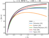 |
Fig. A.1. The rotation velocity v⊥ with various asymmetric drift correction for a galaxy with a Sérsic index ns = 1.5, a NFW profile with Vvir = 100 km/s, cvir = 10, and a velocity dispersion of σ = 30 km/s. |
Appendix B: Parameter degeneracies
Fig. B.1 shows the potential correlations between M⋆ and Mvir from the GALPAK3D DC14 fits. For ID937, which is better fitted by a NFW profile, the fit was restricted to the SED-derived stellar mass M⋆. One sees that, generally, there seems to be a good agreement between the GALPAK3D-derived M⋆ with the SED-derived ones, except for ID943, ID919. The halo mass for ID1002 and the concentration for ID15 are poorly constrained.
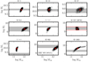 |
Fig. B.1. The M⋆ − Mvir potential correlations from the GALPAK3D fits, derived from the log X − Vvir fits. The horizontal gray band represents the SED-based M⋆ and its 2σ uncertainty. The triangles represent the best-fit values. For ID937, the fit was restricted to the SED M⋆ value. There is good agreement between the GALPAK3D-derived M⋆ with the SED-derived ones, except for ID943, ID919. |
Fig. B.2 shows the potential correlations between cvir and Mvir from the GALPAK3D fits. As in the left panel, the triangles represent the best-fit values. This shows figure shows that the halo concentration is well determined except for ID15 and ID943.
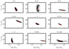 |
Fig. B.2. The cvir − Mvir correlations from the MCMC chain. The triangles represent the best-fit values. One sees that the halo mass for ID1002 and the concentration for IDs15, 943 are poorly constrained. |
Appendix C: Relaxing constraints on α, β, γ
In Fig. C.1, we show the derived α, β, γ parameters using Zhao (1996) DM profile with the 3 parameters (inner & outer slopes, transition sharpness) free. The solid, dotted, dot-dashed lines represent the inner (γ), outer (β) slopes of the DM profile and the sharpness of the transition α as a function of log X = M⋆/Mvir from the DC14 (their Eq. 3). Here, the ratio M⋆/Mvir is degenerate with the profile parameters, so we used the SED stellar mass M⋆, SED as prior.
This figure shows that the DC14 model is not far from the actual DM profiles and indicates that the Dekel et al. (2017) profile with α, β, γ = (0.5, 3.5, γ) (Freundlich et al. 2020b) would be disfavored.
All Tables
All Figures
|
Fig. 1. Stellar continuum postage stamps. HST/F160W flux map for the nine [O II] emitters from the MXDF used in this study (ordered by increasing M⋆ from top left to bottom right). Background and foreground objects have been masked. The ellipse shows a constant isophote on the models. |
| In the text | |
|
Fig. 2. Morpho-kinematics of each SFG. The columns shows (from left to right) the stellar continuum from HST/F160W, the [O II] flux map from MUSE, the [O II] surface brightness profile (SB(r)), the observed projected velocity field (v2d), the observed 1d velocity profile v⊥ sin i, the intrinsic (i.e., deprojected, corrected for beam smearing) modeled rotation curve (v⊥) using the URC model of PSS96 (see Sect. 3.1), and the residuals map obtained from the residual cube (see text). The red solid lines show the intrinsic SB(r) and v⊥ model. The solid black lines show the convolved SB profile and modeled 1d velocity profile. The gray symbols represent the data extracted from the flux and velocity maps. The blue vertical dotted lines represent 2 Re, while the red dotted lines show the radius at which the S/N per spaxel reaches 0.3. |
| In the text | |
|
Fig. 3. Comparison of SED-based stellar masses and kinematic-based stellar masses. The kinematic-based stellar mass M⋆ are obtained from GALPAK3D disk-halo fits, while the SED-based M⋆ are derived from the HST photometry. The error bars represent the 95% confidence intervals. The M⋆ obtained with GALPAK3D (one of the 14 free parameters in Sect. 3.2) and from HST photometry are completely independent, except for ID912 (open circle). The dashed line shows the 1:1 line and this figure shows the two are in excellent agreement, except for ID919 and ID943. |
| In the text | |
|
Fig. 4. Disk-halo decompositions for the nine galaxies in our sample (ordered by increasing M⋆). The solid black line represents the total rotation velocity v⊥(r). All velocities are ‘intrinsic’, that is corrected for inclination and instrumental effects. The dot-dashed line represents the circular velocity vc(r), that is v⊥(r) corrected for asymmetric drift. The gray band represents the intrinsic universal rotation curve (URC) using the parameterization of PSS96 as in Fig. 2. The solid red (blue) line represents the stellar (gas) component v⋆(r) obtained from GALPAK3D modeling of the MUSE [O II] data. The dotted red line represents the stellar component obtained using a MGE decomposition of the HST/F160W stellar continuum images. The green line represents the DM component. The vertical dotted lines are as in Fig. 2. |
| In the text | |
|
Fig. 5. Total stellar-to-halo fraction. Left: total stellar-to-halo fractions M⋆/Mvir as a function of the stellar mass M⋆ obtained from our 3D fits. The error bars from our data are 95% confidence intervals, and the open circles show the sample of Genzel et al. (2020). The shaded (blue contours) histogram shows the location of SFGs in the TNG simulations for z = 1 centrals, while the gray contours show the satellites. The colored lines show the Behroozi et al. (2019) relation inferred from semi-empirical modeling at redshifts z = 0.5, 1.0, 1.5, respectively. Right: total stellar-to-halo fractions M⋆/Mvir as a function of GMvir/j⋆σ⋆ (Eq. (7)) for the galaxies in our sample. The inset histogram shows that the sample has |
| In the text | |
|
Fig. 6. DM fractions for our SFGs. Left: DM fractions within the half-light radius Re, fDM(< Re), as a function of halo mass, Mvir. The dashed line represent the downward trend of Genzel et al. (2020). Right: DM fractions within Re as a function of stellar mass surface density Σ⋆, 1/2 within Re. In both panels, the error bars from our data are 95% confidence intervals, and the open circles show the sample of Genzel et al. (2020). The shaded (blue contours) histogram shows the location of SFGs in the TNG100 simulations for z = 1 central SFGs, while the gray contours show the satellites. The dotted line represents the toy model derived from the TF relation (Eq. (9)). |
| In the text | |
|
Fig. 7. Size of DM cores. Left: halo concentration-halo mass relation. The concentrations cvir for z ≃ 1 SFGs, derived from our 3D modeling of the [O II] rotation curves, are converted to a DM-only NFW equivalent cvir, DMO (see text). Right: DM core size rs, DMO ≡ Rvir/cvir, DMO in kpc as a function of halo mass. The dotted line represents the observed core-mass scaling relation for z = 0 LSBs from Di Paolo et al. (2019) (see text). In both panels, the solid lines represent the cvir − Mvir relation predicted by Dutton & Macciò (2014) for DM halos, color-coded by redshift. The error bars are 95% confidence intervals (2σ) and color-coded also by the galaxy redshift. |
| In the text | |
|
Fig. 8. Halo scale radius-density relation at z = 1. Left: ρs − rs scaling relation for the galaxies shown in Fig. 7. The error bars are 95% confidence intervals (2σ). For comparison, the anticorrelation of Kormendy & Freeman (2004), Spano et al. (2008) and Di Paolo et al. (2019) are shown. Right: DM surface density (Σs ≡ ρs rs) as a function of galaxy mass. The anticorrelation in the left panel implies a constant DM surface density. The gray band represents the range of surface densities from Burkert (2015) for dwarfs. The constant densities of Kormendy & Freeman (2004) and Donato et al. (2009) are shown as the dotted, dot-dashed lines, respectively. |
| In the text | |
|
Fig. 9. DM density profiles in M⊙/kpc3. Each panel show ρdm(r) as a function of r/Re obtained from our disk-halo decompositions (Fig. 4). The stellar-to-halo-mass ratio (log X ≡ log M⋆/Mvir) is indicated. The gray bands represent the 95% confidence interval and the dotted lines represent NFW profiles. The vertical dotted lines represent the 1 kpc physical scale, corresponding to ≈1 MUSE spaxel, and indicates the lower limit of our constraints. |
| In the text | |
|
Fig. 10. Relation between SFR and cores. Left: α, β, γ parameters as a function of log M⋆/Mvir. The curves show the parameterisation of DC14 for α, β, γ and the solid symbols represent our SFGs, excluding ID919 and 943. Middle: DM inner slope γ as a function of the SFR surface density ΣSFR, scaled to z = 1.5. Right: DM inner slope γ as a function of the logarithmic offset from the MS, δ(MS), using the Boogaard et al. (2018) MS. DM cores are present in galaxies with higher SFR and SFR surface-densities. |
| In the text | |
|
Fig. 11. Left: DM density at 150 pc as a function of log M⋆/Mvir. The blue (red) solid circles with error bars (2σ) show our SFGs, except ID919 and 943. Right: DM inner slope γ parameter at 150 pc as a function of log M⋆/Mvir. The blue (red) squares represent the z ≈ 0 dwarfs from Read et al. (2019) whose SFR was truncated less (more) than 6 Gyr ago. The blue (red) solid circles with error bars (2σ) show our SFGs with high (low) ΣSFR, respectively. |
| In the text | |
|
Fig. A.1. The rotation velocity v⊥ with various asymmetric drift correction for a galaxy with a Sérsic index ns = 1.5, a NFW profile with Vvir = 100 km/s, cvir = 10, and a velocity dispersion of σ = 30 km/s. |
| In the text | |
|
Fig. B.1. The M⋆ − Mvir potential correlations from the GALPAK3D fits, derived from the log X − Vvir fits. The horizontal gray band represents the SED-based M⋆ and its 2σ uncertainty. The triangles represent the best-fit values. For ID937, the fit was restricted to the SED M⋆ value. There is good agreement between the GALPAK3D-derived M⋆ with the SED-derived ones, except for ID943, ID919. |
| In the text | |
|
Fig. B.2. The cvir − Mvir correlations from the MCMC chain. The triangles represent the best-fit values. One sees that the halo mass for ID1002 and the concentration for IDs15, 943 are poorly constrained. |
| In the text | |
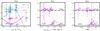 |
Fig. C.1. Same as Fig. 10, but with the ‘Zhao’ DM profiles with free α, β, γ. |
| In the text | |
Current usage metrics show cumulative count of Article Views (full-text article views including HTML views, PDF and ePub downloads, according to the available data) and Abstracts Views on Vision4Press platform.
Data correspond to usage on the plateform after 2015. The current usage metrics is available 48-96 hours after online publication and is updated daily on week days.
Initial download of the metrics may take a while.