| Issue |
A&A
Volume 685, May 2024
|
|
|---|---|---|
| Article Number | A132 | |
| Number of page(s) | 16 | |
| Section | Extragalactic astronomy | |
| DOI | https://doi.org/10.1051/0004-6361/202347243 | |
| Published online | 16 May 2024 | |
Investigating the dark matter halo of NGC 5128 using a discrete dynamical model
1
Max Planck Institute for Astronomy, Königstuhl 17, 69117 Heidelberg, Germany
e-mail: This email address is being protected from spambots. You need JavaScript enabled to view it.
2
Department of Physics and Astronomy, University of Utah, 115 South 1400 East, Salt Lake City UT 84112, USA
3
Department of Physics and Astronomy Michigan State University Biomedical & Physical Sciences, 567 Wilson Rd, Room 3275 East Lansing, MI 48824-2320 Michigan, USA
4
Steward Observatory, University of Arizona, 933 North Cherry Avenue, Tucson, AZ 85721, USA
5
Universite de Strasbourg, CNRS, Observatoire astronomique de Strasbourg, UMR 7550, 67000 Strasbourg, France
6
Steward Observatory, University of Arizona, 933 North Cherry Avenue, Tucson, AZ 85721, USA
7
University of Tampa, 401 West Kennedy Boulevard, Tampa, FL 33606, USA
8
Centre for Astrophysics and Supercomputing, Swinburne University of Technology, Hawthorn, VIC 3122, Australia
9
Department of Astronomy, University of Michigan, Ann, Arbor, MI 48109, USA
10
Center for Cosmology and Particle Physics, Department of Physics, New York University, 726 Broadway, New York, NY 10003, USA
Received:
20
June
2023
Accepted:
21
February
2024
Abstract
Context. As the nearest accessible massive early-type galaxy, NGC 5128 presents an exceptional opportunity to measure dark matter halo parameters for a representative elliptical galaxy.
Aims. Here we take advantage of rich new observational datasets of large-radius tracers to perform dynamical modeling of NGC 5128
Methods. We used a discrete axisymmetric anisotropic Jeans approach with a total tracer population of nearly 1800 planetary nebulae, globular clusters, and dwarf satellite galaxies extending to a projected distance of ∼250 kpc from the galaxy center to model the dynamics of NGC 5128.
Results. We find that a standard Navarro-Frenk-White (NFW) halo provides an excellent fit to nearly all the data, except for a subset of the planetary nebulae that appear to be out of virial equilibrium. The best-fit dark matter halo has a virial mass of Mvir = 4.4−1.4+2.4 × 10¹² M⊙, and NGC 5128 appears to sit below the mean stellar mass–halo mass and globular cluster mass–halo mass relations, which both predict a halo virial mass closer to Mvir ∼ 1013 M⊙. The inferred NFW virial concentration is cvir = 5.6−1.6+2.4, which is nominally lower than cvir ∼ 9 predicted from published cvir–Mvir relations, but within the ∼30% scatter found in simulations. The best-fit dark matter halo constitutes only ∼10% of the total mass at one effective radius but ∼50% at five effective radii. The derived halo parameters are consistent within the uncertainties for models with differing tracer populations, anisotropies, and inclinations.
Conclusions. Our analysis highlights the value of comprehensive dynamical modeling of nearby galaxies and the importance of using multiple tracers to allow cross-checks for model robustness.
Key words: galaxies: general / galaxies: halos / galaxies: kinematics and dynamics
Hubble Fellow.
© The Authors 2024
 Open Access article, published by EDP Sciences, under the terms of the Creative Commons Attribution License (https://creativecommons.org/licenses/by/4.0), which permits unrestricted use, distribution, and reproduction in any medium, provided the original work is properly cited.
This article is published in open access under the Subscribe to Open model.
Open Access funding provided by Max Planck Society.
1. Introduction
Large-scale observations of the Universe show that more than 80% of the total mass in the Universe is in the form of dark matter (e.g., Planck Collaboration VI 2020). At smaller scales, galaxies’ rotation curves derived from neutral hydrogen (HI) observations have also revealed massive dark matter halos in spiral galaxies (e.g., Rubin & Ford 1978; Bosma 1978, 1981; Sofue et al. 1999; Sofue & Rubin 2001; Martinsson et al. 2013). These observations have also shown that the dark matter halo of individual spiral galaxies correlates with their luminosity, stellar mass, and possibly galaxy size (for a more detailed discussion see Wechsler & Tinker 2018).
However, studying the dark matter halos of elliptical galaxies presents a major challenge. Unlike spiral galaxies, which have a disk-like structure rich in HI gas to study their rotation curve, elliptical galaxies do not have sufficient gas for similar measurements. As a result, directly measuring the circular velocities of these galaxies is difficult and instead, we rely on X-ray emission (e.g., Kim & Fabbiano 2013; Forbes et al. 2017), strong lensing (e.g., Auger et al. 2010), or stellar kinematics (e.g., Cappellari et al. 2013b) to determine the distribution of mass in their halos.
At large radii, where stellar kinematics become challenging to derive (Brodie et al. 2014), the use of bright discrete tracers such as planetary nebulae (PNe) and globular clusters (GCs) are a powerful tool to study the galaxy’s gravitational potential (e.g., Zhu et al. 2016; Alabi et al. 2016). PNe are the final evolutionary stage of some low-to-intermediate-mass stars, emitting bright narrow [O III] lines that make them well-suited for spectroscopy at cosmic distances where spectroscopy of individual main sequence or giant stars is infeasible. GCs serve as tracers of the galaxy’s potential extending to even larger radii, providing valuable information about the distribution of dark matter in the outer halo.
NGC 5128, also known as Centaurus A, is among closest and brightest elliptical galaxies to the Milky Way, located at a distance of 3.8 Mpc (Harris 2010). Owing to its proximity, NGC 5128 has been a principal target for the study of GCs and PNe, hosting a rich population of both (Harris et al. 2002, 2004; Martini & Ho 2004; Peng et al. 2004a, 2004b; Woodley et al. 2005, 2007, 2010; Rejkuba et al. 2007; Walsh et al. 2015; Dumont et al. 2022; Hughes et al. 2023). The kinematics of GCs and PNe in NGC 5128 have been used to study the dynamics of the galaxy’s outer halo, providing important insights into the mass distribution in the galaxy (Hui et al. 1995; Peng et al. 2004a; Woodley et al. 2007, 2010; Pearson et al. 2022; Hughes et al. 2023). Published estimates suggest that the total enclosed mass of NGC 5128 is (2.5 ± 0.3) × 1012 M⊙ within ∼120 kpc based on its GC kinematics (Hughes et al. 2023), or (1.0 ± 0.2) × 1012 M⊙ within ∼90 kpc using the PNe as kinematic tracers (Woodley et al. 2007). Based on the modeling of the tidal stellar stream of its dwarf satellite galaxy Dw3 at a projected radius of ∼80 kpc, Pearson et al. (2022) suggest a lower limit for its mass halo of M200 ≥ 4.7 × 10¹² M⊙.
The kinematics and radial density profiles of PNe and GCs are not expected to be the same therefore, using them both as independent kinematic tracers can help break the mass–anisotropy and the luminous-to-dark matter mass degeneracies (e.g., Napolitano et al. 2014). This is especially true in the outer halo of elliptical galaxies such as NGC 5128 that show signs of a complicated merging history (Israel 1998; Wang et al. 2020a). For this work, we used the most current catalogs of available kinematic tracers in NGC 5128 (stellar kinematics, GCs, PNe, and dwarf satellite galaxies), and we modeled them without binning using discrete dynamical models. This approach helps avoid the loss of valuable information (Watkins et al. 2013).
The paper is organized as follows: in Sect. 2, we discuss the kinematic tracers available to constrain our dynamical model. Section 3 provides an overview of the discrete dynamical model employed in this study, including a detailed description of our fiducial model, its assumptions, and free parameters. Section 4 presents the best-fit parameters of the fiducial model, including its dark matter halo and an assessment of the impact of systematics. This model is compared with previous measurements in Sect. 5. Then in Sect. 6, we discuss the implications of our best-fit mass model and how the dark matter halo of NGC 5128 compares to that of other elliptical galaxies.
Throughout this paper, we assume a distance of 3.8 Mpc to NGC 5128 ((m − M)0 = 27.91; Harris et al. 2002). At this distance, 1′≈1.1 kpc. We also assume that the photometric major axis (PA) is 35° east from north based on results of Silge et al. (2005), a systemic velocity for NGC 5128 of 540 km s−1 based on results from Hughes et al. (2023), and an effective radius of Reff = 305″ adopted from Dufour et al. (1979).
2. Kinematic tracers
In this section we describe the available kinematic data for NGC 5128 used to constrain our dynamical mass models. There are a total of 1267 PNe line-of-sight (LOS) velocities compiled by Walsh et al. (2015), 645 confirmed GCs with LOS velocities compiled by Hughes et al. (2023), and LOS velocities for 28 satellite dwarf satellite galaxies (Crnojević et al. 2019; Müller et al. 2021). We describe these samples each in greater detail below.
The 1267 spectroscopically confirmed PNe with radial velocities compiled by Walsh et al. (2015) also include measurements from previous works (Hui et al. 1995; Peng et al. 2004a), which have larger velocity errors. For our dynamical models, we only consider the 1135 PNe with smaller errors, as described in more detail in Walsh et al. (2015). The median projected galactocentric radius of the PNe is 9 kpc with some objects as far out as 39 kpc. Typical velocity errors are 1.7 km s−1. The kinematics of the PNe are complex with rotation around the minor axis at small radii, but with a changing axis of rotation at large radii that suggest either non-virial motions or a triaxial potential; their kinematics are discussed in detail in Peng et al. (2004a).
The largest, most up-to-date catalog of GCs in NGC 5128 is presented in Hughes et al. (2023). This cluster catalog includes 122 new measurements and compiles measurements of 523 additional literature GC velocities from a wide range of sources (Graham & Phillips 1980; van den Bergh et al. 1981; Hesser et al. 1986; Harris et al. 2002, 2004; Peng et al. 2004b; Martini & Ho 2004; Woodley et al. 2005, 2007, 2010; Rejkuba et al. 2007; Beasley et al. 2008; Georgiev et al. 2009; Taylor et al. 2010, 2015; Voggel et al. 2020; Fahrion et al. 2020; Dumont et al. 2022). The newly discovered GCs from Hughes et al. (2023) extend to larger radii than previous measurements, with the full sample having a median radius of 17.8 kpc and a maximum radius of ∼130 kpc. The dataset has both low and high resolution measurements, with median velocity errors of 29.5 km s−1. The 523 literature objects are a smaller number than the catalog of 563 GC velocities in Woodley et al. (2010) due to the discovery that many previous GC candidates were foreground stars based on Gaia measurements and subsequent velocity measurements (Hughes et al. 2021, 2023; Dumont et al. 2022).
The GC population of NGC 5128 can be divided into metal poor GCs (referred to as “blue”) and metal rich GCs (referred to as “red”), which have distinct spatial distributions. For our dynamical models, we treat the blue and red GC populations as separate kinematic tracers. We adopt the same classification for red and blue GCs as used in Hughes et al. (2023), which is based on their (u − z)0 and (g − z)0 color. Specifically, we separate GCs with (u − z)0 < 2.6 or (g − z)0 < 0.65 as blue GCs, with GCs above these colors as red GCs. Nine GCs with velocities lacked color information and are not used in our analysis. Additionally, Hughes et al. (2023) identifies 18 GCs associated with either dwarf satellite galaxies or with other stellar streams. For our fiducial model we fit red and blue GCs separately, and exclude GCs associated with stellar substructures as these give multiple measurements for a single dynamical tracer. In total we fit 618 GCs, 279 red GCs and 339 blue GCs.
NGC 5128 hosts 42 confirmed dwarf satellite galaxies (hereafter referred to as “dwarfs”), as compiled in Crnojević et al. (2019) and Müller et al. (2021), with 28 of them having LOS velocities. We are only interested in fitting satellite galaxies that are located within the virial radius of NGC 5128, rather than orbiting in the larger group potential. Previous measurements suggested a virial radius in the range 200–300 kpc (Peng et al. 2004a; Müller et al. 2022); therefore, we limit our sample to the 16 satellite galaxies with projected distances of ≤250 kpc. The LOS velocities of our three kinematic tracers (PNe, GCs, and dwarf satellite galaxies) are shown in Fig. 1.
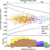 |
Fig. 1. Radial distribution of the LOS velocity for the PNe (yellow), metal rich, and metal poor GCs (red and blue respectively), and the dwarf satellite galaxies (green) around NGC 5128. The LOS velocities are with respect to the systemic velocity of NGC 5128 of 540 km s−1 (Hughes et al. 2023). The solid black line shows the radial profile for the escape velocity for NGC 5128 derived from our best-fit mass model including dark matter presented in Sect. 4.1, while the dashed lines shows the escape velocity for just the stellar mass. The bottom panel is a histogram with the radial distribution for the PNe, GCs and dwarfs in the same colors as the top panel. |
Finally, we note that there is available stellar kinematic data for NGC 5128 itself from several different sources for the innermost regions of the galaxy (e.g., Silge et al. 2005; Cappellari et al. 2009). Given that our primary interest is in the mass distribution at larger radii, we do not explicitly model these central data. Instead, we fix the inner (≤180″) K-band mass-to-light ratio based on the results from the stellar kinematic modeling of Cappellari et al. (2009). A more detailed discussion on this is presented in the next section (Sect. 3.1).
3. Discrete dynamical modeling
In this section, we introduce the discrete dynamical modeling approach that we use to estimate NGC 5128’s dynamical mass and dark matter halo properties. We subsequently discuss the input ingredients, including models of the gravitational potential, the density profiles of each kinematic tracer, the log-likelihoods used to estimate the best-fit parameters, and finally, the Markov-chain Monte Carlo (MCMC) method used for parameter estimation.
We consider that the PNe, GCs (blue and red), and dwarf satellite galaxies are independent populations, each with their own spatial and dynamical properties, whose kinematics trace the same underlying gravitational potential. We model the dynamics of each population with an axisymmetric anisotropic Jeans model (as implemented in the axisymmetric version of the Jeans Anisotropic Modeling software JAM; Cappellari 2008). The discrete kinematic tracers are modeled directly without binning to avoid loss of information, following the discrete maximum-likelihood modeling approach extension to the JAM software (CJAM) introduced by Watkins et al. (2013). CJAM predicts the full three-dimensional matrix of the first and second velocity moment as a function of the major and minor axes position (x′ and y′) of the discrete kinematic tracer. Our kinematic tracers do not have available proper motions but only LOS velocity, so we only use the LOS (z′) component of the CJAM to constrain our models. This model assumes that the velocity ellipsoid of the kinematic tracers is aligned with the cylindrical coordinates (x′, y′, z′). CJAM requires the following properties as input:
– The gravitational potential profile in the form of an elliptical multi-gaussian expansion (MGE; Cappellari 2002). For our models we assume the gravitational potential is formed from the combination of luminous matter and dark matter (see more details in Sect. 3.1).
– A mass-to-light ratio (ΥK) that converts the stellar luminosity profile into a stellar mass profile.
– The projected density profile for each kinematic tracer, also expressed in the form of an MGE.
– The global inclination of the system i, which we assume to be i = 90° or edge-on. While a common simplifying assumption in dynamical studies of early-type galaxies (e.g., Zhu et al. 2016), it is specifically supported for NGC 5128 by previous dynamical work on the PNe population (Hui et al. 1995; Peng et al. 2004a). However, we do explore the impact of the assumed inclination in Sect. 4.3.3.
– A rotation parameter κ for each kinematic tracer, as defined in Eq. (35) in Cappellari (2008). We assume κ to be zero (no rotation) to reduce computing time (see additional discussion in Sect. 4.1.3).
– A velocity anisotropy parameter  (defined in cylindrical coordinates; called βz in Cappellari et al. 2009), which takes negative values for tangential anisotropy and positive values for radial anisotropy. The β can be separately specified for each tracer MGE component.
3.1. Gravitational potential
We model the gravitational potential of the galaxy assuming it is made by two components: a luminous and dark matter component. We model the luminous mass potential by assuming mass follows light, characterizing its surface brightness profile (Sect. 3.1.1), and fitting for a mass-to-light ratio. For the dark component (Sect. 3.1.2) we assume it follows a generalized Navarro–Frenk–White (NFW) density profile (Navarro et al. 1996; Zhao 1996).
3.1.1. Stellar gravitational potential
We characterize the contribution of luminous mass to the gravitational potential in our dynamical models by deriving the galaxy’s surface brightness profile and multiplying this by a mass-to-light ratio to convert it into a mass profile. We derive the central surface brightness profile of NGC 5128 using data from the 2MASS Large Galaxy Atlas imaging data (Jarrett et al. 2003). We use the Ks-band mosaic for NGC 5128 since it is sensitive to the main, primarily old stellar population and is less affected by dust extinction than images at shorter wavelengths. The 2MASS imaging data extends to approximately ∼200″ from the galaxy center. However, there is observational evidence that luminous matter contributes significantly to the gravitational potential of the galaxy inside ∼10 kpc, or ∼600″ (Peng et al. 2004a), beyond the sensitivity limit of the 2MASS images.
To characterize the outer stellar halo, we turn to previous literature measurements by Dufour et al. (1979) and Rejkuba et al. (2022), and combine their outer surface brightness profile data with the 2MASS Ks image at smaller radii. Dufour et al. (1979) derived a V and B surface brightness profile from unresolved stars using photographic plates out to a radius of ∼8′ centered on the nucleus of NGC 5128. Dufour et al. (1979) found that the galaxy’s V-band surface brightness profile is well represented by a de Vaucouleurs’s law at radial distances between 70″ and 255″. Because we are deriving the surface brightness profile in the 2MASS Ks band, we need to convert this profile using a V − Ks color. Based on PARSEC single stellar population models (Marigo et al. 2017), we expect a V − Ks ∼ 3 for old age populations at somewhat subsolar metallicities. This color provides a good overlap between the outer part of the 2MASS image and the inner part of the Dufour et al. (1979) profile (70″), and we assume this color for both this profile (μK in Eq. (1)) and to convert the Rejkuba et al. (2022) profile below. The V and Ks profiles from Dufour et al. (1979) that we use is thus:
![Mathematical equation: $$ \begin{aligned} \begin{aligned}&\mu _{\mathrm{K}} = 8.32[(a/R_{\rm eff})^{1/4} - 1] + 22.0 - 3.0, \end{aligned} \end{aligned} $$](/articles/aa/full_html/2024/05/aa47243-23/aa47243-23-eq4.gif) (1)
(1)
where Reff = 305″(∼5.6 kpc) is the effective radius of NGC 5128, a = x′2 + y′2/(1 − e)2 is the major axis distance, and the mean ellipticity of NGC 5128 is e = 1 − (b′/a′) = 0.23, where b′/a′ is the minor-to-major axis ratio (Dufour et al. 1979).
Rejkuba et al. (2022) derive a number density profile of resolved red giant branch (RGB) stars from a large number of archival Hubble Space Telescope fields in the outer halo of NGC 5128 extending to radii of ∼140 kpc. They fit this data to a de Vaucouleurs-Sérsic profile, and provide a conversion from number density to V-band surface brightness. Specifically we use equation 13 from Rejkuba et al. (2022):
 (2)
(2)
where ΦRGB is the number density of RGB stars per arcmin−2. We then need to convert Eq. (2) from counts per arcmin−2 to Ks-band surface brightness to provide a uniform band for our input mass-model. Using the conversion given by Rejkuba et al. (2022) of log(ΦRGB)=0 is equal to a V-band surface brightness of μV = 33.82 mag arcsec−2 and assuming V − Ks = 3 mag, the resulting Ks-band surface brightness profile in units of mag arcsec−2 is:
 (3)
(3)
We assume a PA = 35° for the two outer halo surface brightness profiles. This is the PA found for the 2MASS image in Silge et al. (2005) and also is consistent with the PA found by Dufour et al. (1979). We use an ellipticity for both outer halo profiles of e = 0.23, while the ellipticity in the inner part is fitted from the 2MASS data. This PA and ellipticity are different from the best-fit values in Rejkuba et al. (2022) of PA =55° and e = 0.46 ± 0.02 – we note however that their values are not based on azimuthally complete data, but instead are a best-fit to isolated HST fields that sample only a small portion of the outer halo. While it is possible that the PA twists at large radii, our CJAM modeling cannot accommodate such a twist. We therefore use the Dufour et al. (1979) values of PA and e throughout the halo.
We combine the profiles by creating a single image combining the 2MASS data at small radii (< 70″), and the Dufour et al. (1979) (for distances between 70 − 255″) and Rejkuba et al. (2022) profiles at large radii (beyond 255″). To do this, the two halo surface density profiles (Eqs. (1) and (3)) have to be transformed back into counts using the 2MASS K-band zeropoint (ZPKs = 19.915 mag) to be combined with the 2MASS image. The resulting combined image is fit using an MGE model, assuming a point-spread function (PSF) of 1.3″ determined by measuring the full width at half maximum (FWHM) of stars in the 2MASS image. The resulting final major axis surface brightness profile and the sum of the fitted MGEs are shown in Fig. 2, and the MGE parameters are listed in Table 1. We note the axis ratios for the MGE components are left as free parameters; since each component has contributions from a range of radii, they do not exactly equal the value assumed for the outer halo in constructing the combined surface brightness profile. We calculate the total K-band luminosity of NGC 5128 by integrating the three-dimensional Gaussian with amplitude, sigma and flattening based on the Luminous MGEs listed in Table 1. We find a total K-band luminosity of 1.544 × 10¹¹ L⊙ which is in excellent agreement with the results found by Karachentsev et al. (2002).
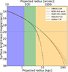 |
Fig. 2. Stellar surface brightness profile of NGC 5128. This figure shows a comparison between the best-fit MGE model for the surface brightness (red) with the 2MASS Large Galaxy Atlas surface brightness profile (blue) Jarrett et al. (2003), literature MGE model of NGC 5128 (dashed black line) by Häring-Neumayer et al. (2006), and the outer halo profiles in the V-band by Dufour et al. (1979) and Rejkuba et al. (2022) (green and yellow respectively), assuming a V − Ks = 3 mag. The blue horizontal dashed line represents the 2MASS surface brightness 1σ noise level used to derived the most inner part of the MGE model. The vertical bands show the radius at which we use the 2MASS K-band image, the de Vaucouleurs-Sérsic profile by Dufour et al. (1979) and Rejkuba et al. (2022) respectively to derive the MGE model shown in red. |
MGE parametrization of NGC 5128.
Using this MGE, CJAM can deproject the two-dimensional MGE model into a three-dimensional profile. Multiplied by a mass-to-light ratio, we get a luminous stellar mass density.
Perhaps surprisingly, there has been no published analysis of the star formation history of the inner few kpc of NGC 5128 based on integral-field spectroscopy or similar methods that would allow us fine-grained constraints on the mass-to-light ratio as a function of radius. However, Hubble Space Telescope/WFC31 images for NGC 5128 clearly show the presence of young stars and ongoing star formation inside the dust ring of NGC 5128, which extends out to ∼180″. Beyond this radius the light appears to be dominated by an older smoother component extending outward through the halo. Because our tracer population is primarily located at large radii, and our interest is in constraining the outer mass profile of the galaxy, we fix the inner (all MGE components with spatial σ ≤ 180″) to ΥK = 0.65 based on results from Cappellari et al. (2009). They used VLT/SINFONI stellar integrated field spectroscopic data in the nuclear regions, and found good agreement with spectroscopy extending out to ∼40″. We then leave the ΥK for the outer halo (i.e., all MGE components with σ > 180″) as a free parameter in our models. We note that Bílek et al. (2019) use stellar population models applied to the integrated B − V colors of NGC 5128 and find a B-band mass-to-light ratio of ΥB ∼ 3 ± 0.5; translating the Cappellari et al. (2009)ΥK = 0.65 to B-band, we find rough agreement, with ΥB ∼ 2.42
3.1.2. Dark matter gravitational potential
For the dark matter contribution to the gravitational potential, we assume a generalized version of the Navarro-Frenk-White (NFW) density profile (Navarro et al. 1996; Zhao 1996):
 (4)
(4)
with rs being the scale radius in pc, ρs the scale density in M⊙/pc3, γ and η are the inner and outer density slope. For most models presented here, we assume γ = η = 1, the standard NFW profile from Navarro et al. (1996). We also assume a spherical halo, an assumption shared by previous measurements of the dark matter halo of NGC 5128 (e.g., Peng et al. 2004a). While the true shape of the halo is likely somewhat triaxial (e.g., Hui et al. 1995; Peng et al. 2004a; Veršič et al. 2023), the main stellar body of NGC 5128 has a relatively modest ellipticity, and numerical simulations show that dark matter halos are typically rounder than luminous matter in giant elliptical galaxies (e.g., Wu et al. 2014). However, future works could use instead NGC 5128’s stellar streams to constraint the dark matter halo shape as done for the Milky Way (Nibauer et al. 2023), expanding on current modeling of NGC 5128’s stellar streams done by Pearson et al. (2022).
We approximate the NFW profile with an MGE model (extending up to 3× further out than our furthest GC); because the NFW profile is a 3D density, we obtain the height of the best-fit 1D Gaussians and multiply these by  to convert these to the equivalent 2D Gaussians expected by CJAM.
3.2. Tracer density profiles
Each kinematic tracer has its own projected density profile, and CJAM uses this profile to translate the projected position into a distribution of 3D positions that is needed to estimate their velocity moments.
3.2.1. Globular cluster density profiles
Metal rich (red) and metal poor (blue) clusters have been typically found to have different spatial and kinematic distributions in both the Milky Way and many other galaxies, with the red GCs being more centrally concentrated and the blue GCs more extended (e.g., Brodie & Strader 2006). For the spatial distributions of these subpopulations, we use the power law fits to the confirmed blue and red GCs in NGC 5128 from Hughes et al. (2023) fit over a range of 7–30′ (∼7.7 − 33 kpc). They find that the red GC population has a steeper profile with a best-fit power law slope of −3.05 ± 0.28, while the blue GC population has a slope of −2.69 ± 0.27.
For each GC subpopulation, we create a radial surface density profile (in units of number/arcmin2) up to a radius of 5.5° (∼370 kpc), well beyond the boundary of our observed GC population. We fit this profile with an MGE model assuming spherical symmetry. The MGE surface density model is then deprojected into a three-dimensional profile (with units of volume density).
3.2.2. Planetary nebulae density profile
Since PNe are just dead low-mass stars, we assume they follow the distribution of the main stellar population of NGC 5128. Thus, for their tracer density profile, we just use the MGE surface brightness profile derived in Sect. 3.1.1.
3.2.3. Satellite galaxy density profile
The number density profile for dwarfs can be obtained using the whole sample of 42 confirmed dwarf satellite galaxies combining Table 6 from Crnojević et al. (2019) with Table A.1 from Müller et al. (2021). To avoid binning the data to fit a power law in such a small sample, we fit instead a power law to the cumulative probability distribution function of the projected radii of the satellite population (e.g., Carlsten et al. 2020). We are only modeling the kinematics of satellite galaxies at ≤250 kpc and therefore fit the 29 satellite galaxies within this radius (this is higher than the 16 used in our dynamical modeling, since only a subset of these 29 have measured radial velocities). The best-fit cumulative power law slope is 1.47 ± 0.23, with the uncertainty derived from bootstrapping. A cumulative distribution power law index of 1.47 ± 0.23 implies a two-dimensional radial density profile (equivalent to the probability distribution function) slope of −0.53 ± 0.23. This measurement is consistent with the flat surface profiles for dwarf satellite galaxies observed in other nearby galaxies, such as M31 (e.g., Doliva-Dolinsky et al. 2023). We use this power law slope to create a radial surface density profile and fit it with a MGE model that we subsequently deproject into a three-dimensional profile.
3.3. Tracer log-likelihoods
Our CJAM models use the number density MGEs and the gravitational potential MGE to predict the first and second-velocity moments of the kinematic tracers. Using a maximum-likelihood analysis we can compare the CJAM LOS velocity predictions directly with our data. Assuming a Gaussian velocity distribution for the GCs, PNe and dwarf satellite galaxies, a point i with coordinates (x′, y′, z′) has a dynamical probability of:
![Mathematical equation: $$ \begin{aligned} P_{\mathrm{dyn},i} = \frac{1}{\sqrt{\sigma _{i}^{2} + \delta v_{z^{\prime },i}^{2}}} {\exp }\left[-\frac{1}{2}\frac{(\delta v_{z^{\prime },i} - \mu _{i} )^{2}}{\sigma _{i}^{2} + \delta v_{z^{\prime },i}^{2} }\right], \end{aligned} $$](/articles/aa/full_html/2024/05/aa47243-23/aa47243-23-eq9.gif) (5)
(5)
where μi and σi are the LOS mean velocity (vc from CJAM) and velocity dispersion ( from CJAM) predicted by our CJAM dynamical models.
Since the GCs, PNe and dwarf satellite galaxies are independent tracers (but modeled with the same gravitational potential), each population has separate probabilities, giving a total log-likelihood:
 (6)
(6)
where GC, PNe, and Dwarfs are used for our globular cluster, planetary nebulae and dwarf satellite galaxy tracers.
3.4. Markov chain Monte Carlo optimization
To effectively explore the parameter space of our discrete dynamical models we use a MCMC implementation. We use the PYTHON software EMCEE (Foreman-Mackey et al. 2013) for an affine-invariant MCMC ensemble sampler. For the proposed distribution of the walkers we used a combination of two moves, DESnookerMove with an 80% weight and DEMove with a 20% weight, effectively meaning that the walkers will choose 80% of the times the DESnookerMove proposal and 20% of the times the DEMove proposal. This combination of proposals for the walkers is suggested in the documentation of EMCEE for “lightly” multimodal model parameters (more details about the DESnookerMove and DEMove can be found in the references within the EMCEE documentation3). We use this mixture of walker proposals as it has already been tested for multimodal parameters and we found it improves the convergence of our models relative, for example, to the default “stretch move”.
For each model, we use the double amount of walkers as the number of free parameters in the model, and run EMCEE for 1000 steps. Based on analysis of the auto-correlation functions, we discard the first 200 steps as burn in and use the remaining 800 steps to characterize the post-burn distribution of the free parameters.
3.5. Fiducial dark matter halo model
For the fiducial model (capitalized for clarity throughout), we use the full sample of tracers as discussed in Sect. 2. The model assumes each tracer has its own anisotropic orbital distribution. For the dark matter halo, we assume an NFW profile for the dark matter component. In total, there are seven free parameters:
-
1.
K-band stellar mass-to-light ratio (ΥK) outside a radius of 180″ (see additional discussion below).
-
2.
Logarithm of the dark matter scale density, log(ρs).
-
3.
 . This is a proxy for the dark matter scale radius rs that is the parameter of interest, but fitting for log(Ds) rather than rs reduces the degeneracy between ρs and rs.
 -
4.
Four β velocity anisotropy parameters, one for each different tracer: red GCs (βred), blue GCs (βblue), PNe (βPNe), and dwarf satellite galaxies (βdwarf).
As mentioned in Sect. 3.1.1, we fix ΥK = 0.65 for the inner 180″, based on results of Cappellari et al. (2009). However, we leave ΥK as a free parameter for radius beyond 180″ with a Gaussian prior of 1.08 ± 0.30 based on the distribution of dynamical stellar ΥK of early-type galaxies from the ATLAS3D project (Cappellari et al. 2011).
For the free parameters in the NFW profile, we use a Gaussian prior for their corresponding virial concentration cvir = rvir/rs, where rvir is the virial radius (see Sect. 4.1). We set this Gaussian prior using the relation between concentration and the virial mass cvir = 15−3.3 log(Mvir/1012 h−1 M⊙) from the simulations of Bullock et al. (2001). With an assumed Mvir = 1.3 × 10¹² M⊙ for NGC 5128 from Woodley et al. (2007), we get a mean concentration cvir = 14.0 with a standard deviation of 5.6 calculated from the 40% scatter in the Bullock et al. (2001) relation. Anticipating our final results, we find a higher virial mass (and hence lower expected cvir) for NGC 5128, but the broad nature of this prior allows the likelihood to dominate in our modeling.
We use a uniform prior from −0.4 to 0.4 for the anistropy parameters at all radii for βred, βblue, βdwarf. We use this same prior for βPNe, but this parameter only applies outside of 180″. Inside 180″, we set βPNe to the published radial velocity anistropy profile from the stellar kinematic fits of Cappellari et al. (2009; βPNe = −0.35 for R ≤ 0.5″, βPNe = 0.2 for 0.5″ < R ≤ 10″, and βPNe = −0.35 for 10″ < R ≤ 180″). We verify that this anisotropy profile provides a good fit to the central stellar kinematics described in Sect. 2.
4. Dynamical modeling results
In this section, we fit our fiducial dynamical model to the data and summarize the results (Sect. 4.1). We then explore the sensitivity of these results by varying the data fit (Sect. 4.2) and different model assumptions (Sect. 4.3).
4.1. Fiducial model results
The MCMC implementation of the fiducial model consists of 14 walkers with 1000 steps. The MCMC converges after 200 steps, and the post-burn probability distribution functions (PDFs) for each parameter are shown in the left side of Fig. 3 and Table 2.
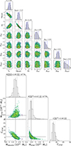 |
Fig. 3. Top: MCMC post-burn distribution for the seven free parameter of the fiducial model. The histograms show their marginalized PDF, and the vertical blue lines show their best-fit value and their 1-σ error. The scatter plots show the two-dimensional PDF for the parameters colored by log-likelihood, with yellow colors indicating higher values. The red-dashed lines indicate each parameter’s best-fit value (median) location, and the black-dashed contours show their 1-σ and 2-σ error. Bottom: plots show the one and two-dimensional PDF distribution for Mvir, M* and cvir. Lines and contours in this plot are the same as in the left panel, but all are shown here in black. |
Mass modeling results.
Most of the parameters are well-constrained by the data. We observe correlations between the stellar mass-to-light ratio ΥK (which determines the mass in stars) and the NFW profile parameters. Specifically, ΥK has a negative correlation with log10ρs with a Spearman coefficient of rSpearman = 0.8, and positive correlation with Ds with rSpearman = 0.6. Such correlations are expected: our dynamical tracers constrain the total mass, and thus a more massive luminous component will require a less massive dark matter halo component (and vice versa).
While the use of  as a proxy for the NFW scale radius rs partially helps break the degeneracy between ρs and rs in the fits, we still observe a negative correlation between log(Ds) and log(ρs) with a Spearman coefficient of rSpearman = 0.9. This is also expected given that both parameters contain ρs. In any case, both NFW halo parameters are well-constrained by the data. All parameter estimates quoted below are calculated as the median of the posterior PDF, with the listed uncertainties corresponding to 1σ equivalent (68%) of the PDF around the median.
4.1.1. Dark matter halo parameters
For the NFW scale parameters, we find a  and
and  kpc, with the latter derived from log(Ds). To more directly compare our results with published values and with simulations, we calculated the corresponding virial mass (Mvir), virial concentration (cvir), and luminous mass (M*) based on our best-fit parameters shown in Fig. 3 (left). We show these translations for each of our MCMC walkers in Fig. 3 (right) and Table 3.
Mass modeling derived quantities.
We define Mvir as the mass enclosed at a radius (virial radius rvir) where the mean halo density ( ) is δth × Ω0 times the critical density (ρcr) of the universe at that redshift. δth is the density contrast of a collapsed object in the “top-hat” collapse model, and Ω0 the matter contribution relative to the critical density. To calculate ρcr, δth and Ω0 we use the ASTROPY.COSMOLOGY python class (Astropy Collaboration 2013) with the cosmology based on the Planck mission (Planck Collaboration XIII 2016). At the redshift of NGC 5128 (z = 0.001834) we get ρcr = 1.27 × 10⁻⁷ M⊙/pc3, δth = 331.50, and Ω0 = 0.308. Finally, Mvir is given by:
 (7)
(7)
We emphasize the difference between Mvir, cvir, and rvir with the also commonly use quantities M200, C200, and R200 calculated for a mass enclosed at the distance 200 × ρcr regardless of the redshift. At this redshift M200 ∼ 0.8 × Mvir.
Our fiducial model fit has a dark matter halo virial mass of  , a concentration of
  , and a corresponding virial radius of
  kpc. Using the best-fit ΥK (see Sect. 4.1.2), the total baryonic mass of the fiducial model is
  . This gives us a total mass (Mvir, t = Mvir + M*) of
  . We note Mvir, t is calculated from the joint distribution of Mvir and M*, and thus does not represent a simple sum of these two estimates. To facilitate comparison with other studies, we also calculated other commonly used quantities referenced to a cosmological overdensity of Δ = 200. Our fiducial model gives
  and
and  , corresponding to a total mass of
  . These quantities are smaller than the virial ones; at z = 0, M200 ∼ 0.8 Mvir. The fiducial model has a dark matter fraction fDM of 0.11 ± 0.04 within 1reff and 0.52 ± 0.08 within 5reff.
4.1.2. Mass-to-light ratio
We determined a best-fit value of  for the mass-to-light ratio in the outer region of NGC 5128 (> 180″; ≳3.3 kpc).We can approximately convert ΥK to a B and V-band mass-to-light ratio of ΥB = 5.5 and ΥV = 4.3, using the same conversion as described at the end of Sect. 3.1.1. The ΥV value is in good agreement with expectations from stellar population models (Bruzual & Charlot 2003) for the old and metal rich populations found in NGC5128’s halo (Rejkuba et al. 2011).
Our best-fit value for ΥK is about 2.5 times larger than the ΥK = 0.65 found by Cappellari et al. (2009) for the inner regions of the galaxy (≲0.7 kpc), and more than 1σ larger than the prior value of ΥK = 1.08 ± 0.3 assumed in our dynamical models (see Sect. 3.5).
Given that we expect the outer stellar regions of NGC 5128 to be older than the inner regions, it is not surprising that the ΥK value fit in the outer regions is larger. However, it also lies at the upper edge of the values favored by our prior, perhaps suggesting a tension between the data and the prior. There are several potential solutions to this discrepancy. First, simulations conducted by Li et al. (2016) suggest that JAM dynamical models tend to overestimate the baryonic mass and underestimate the inner dark matter content in triaxial galaxies. Since some previous studies found evidence that NGC 5128 is triaxial (Hui et al. 1995; Peng et al. 2004a), this could in principle explain the overestimation of the baryonic mass and hence a too-high ΥK. Another, perhaps more likely possibility is that the tracers in the inner, more baryon-dominated regions are not in virial equilibrium due to the residual effects of a major merger (Wang et al. 2020a; see additional discussion in Sect. 4.2).
4.1.3. Tracer anisotropy
In our model fits, all tracers nominally exhibit tangential velocity anisotropy, but this is statistically significant only for the red and blue GCs, both of which have β ∼ −0.3. The PNe are very mildly anisotropic (β ∼ −0.11 ± 0.08) and the dwarf satellite galaxies are close to isotropic, though the anisotropy is poorly constrained for the latter due to small numbers. We provide more detailed analysis of the velocity anisotropy profiles for each tracer in Sect. 4.3.2.
We note that the observed appearance of velocity anisotropy depends on inclination. As in previous dynamical modeling of both NGC 5128 (e.g., Hui et al. 1995; Peng et al. 2004a) and other galaxies (e.g., Zhu et al. 2016), we assume an edge-on inclination in our modeling. We investigate this assumption in more detail in Sect. 4.3.3.
A caveat on the precise values of anisotropy inferred is that previous studies have shown significant rotation for both the PNe (Peng et al. 2004a; Woodley et al. 2007; Coccato et al. 2013) and the metal poor and metal rich GCs (Woodley et al. 2007, 2010; Coccato et al. 2013; Hughes et al. 2023). We experimented with the inclusion of rotation in our models, but in the end chose not to simultaneously model both anisotropy and rotation due to the computational expense. While this is not expected to affect the mass estimates, since the total enclosed mass depends on Vrms, which remains the same whether rotation is included or not in our models, the inclusion of rotation in the models could change the inferred anisotropy for the tracers. This is an interesting potential degeneracy to investigate in future work.
4.1.4. Velocity dispersion profiles: comparing model and data
In Fig. 4 we present a visual comparison of our fiducial model to the tracer observations. Focusing first on the data, the outlined white points represent the observed tracer velocity dispersion measurements binned using a maximum likelihood estimator from Walker et al. (2009) with errors calculated using bootstrapping. This velocity dispersion is equivalent to the observed Vrms, since it includes no rotation component and is azimuthally averaged. The Vrms for the blue GCs remains mostly constant with radius with values around Vrms ≈ 140 km s−1, while for the red GCs there is a slow decrease of Vrms with radius, considering the large uncertainty the Vrms stays mostly constant with radius at Vrms ≈ 130 For the PNe, Vrms is highest in the center at ≈160 km s−1, but shows an abrupt drop at around 1reff and non-monotonic variations at larger radii. These features may be related to the possibilities of non-virial motions or triaxiality discussed above.
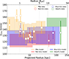 |
Fig. 4. Comparison of observed Vrms radial profiles for the different kinematic tracers (outlined points) to predicted profiles from our best-fit fiducial dynamical model (colored rectangles). The colors represent the same tracers as in Fig. 1. This figure shows that the fiducial model does an excellent job of explaining the overall velocity distribution of our tracers. |
To compare these measurements to the model, we derive predicted Vrms profiles for our fiducial model for each of the individual tracers. The model values were evaluated at the same points as the data in each radial bin. The models are shown as colored rectangles, with the height on these rectangles indicating the standard deviation in the modeled Vrms values due to the radial and azimuthal variation of data points within each bin. We note that the binning in Fig. 4 is solely for the purposes of this comparison–all dynamical modeling fits were made to unbinned data.
We generally find good agreement between the data and model predictions in Fig. 4, with the shaded data regions for each tracer consistent with model predictions. Hence our NGC 5128 mass model appears to be a reasonable fit to the observed tracer populations.
In the next two subsections we explore the robustness of our model fits by exploring their dependence on (i) the details of the datasets used and (ii) the model assumptions.
4.2. Checking robustness: data variations
We begin by separating the classes of tracers (GCs, PNe, and dwarfs) and fitting the same class of model as for our fiducial model: a stellar + anisotropic NFW halo model, fit to each class of tracers individually. The results of these fits are listed in Table 2 and plotted in Fig. 5.
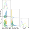 |
Fig. 5. One-and two-dimensional PDF of Mvir, cvir, and M* of the fiducial model compared to the PDF inferred from single-tracer anisotropic models. The blue PDF represents the GC-only model, the yellow PDF the PNe-only model, and the green PDF the dwarfs-only model. We represent 1-σ and 2-σ confidence intervals for each model with darker and lighter colors, respectively. The dashed lines show the median value for each quantity for the fiducial model, and they are the same as in Fig. 3 on the top. |
Focusing first on the inferred halo parameters, the concentration cvir and virial mass Mvir measured from the GCs are consistent with the fiducial model within the uncertainties. The same is true for the dwarfs, though the dwarfs cvir is poorly constrained owing to small numbers and their restricted radial range. However, the derived halo parameters from the PNe are drastically different than the fiducial model, with a much more concentrated and less massive halo (cvir = 18 ± 4;  ).
).
This tension does not appear to be driven by differences in the inferred anisotropy for the tracers. The anisotropy of the red and blue GCs were essentially identical to those in the fiducial model, while that of the PNe is marginally more negative, but not to a sufficient degree to explain this discrepancy. In Sect. 4.3.2 below we explore whether allowing radial variations in the anisotropy could relieve the tension between GCs and PNe. Anticipating these results, we do not find significant observational support for such variations.
The stellar masses (M*) inferred from the separate tracer fits all agree within 1σ with the fiducial model and with each other. However, the three single-tracer models find a smaller ΥK than the fiducial model, yielding less mass in stars and more in dark matter at these inner radii. This is the expected degeneracy between the apportionment of mass between stars and dark matter, and the advantage of the fiducial model is that using a range of tracers with different radial distributions helps to partially break this degeneracy.
As mentioned above, several previous papers have shown that the PNe display complex kinematics, with minor axis rotation at small radii and major axis rotation at larger radii. Peng et al. (2004a) suggested this could be due to triaxiality. Axisymmetric JAM modeling of triaxial systems has been studied by Li et al. (2016); they find that the impact compared to spherical models is only about 20% in mass, much lower than the discrepancies we see between the PNe and GCs. A more straightforward interpretation of these results is that at least a subset of the NGC 5128 PNe are not virialized, likely due to the recent merger (Israel 1998; Wang et al. 2020a), consistent with the findings of Coccato et al. (2013). This has also been observed in the PNe of other recent-merger elliptical galaxies, such as M94 (Hartke et al. 2018). Recent mergers could also affect the orbits of the GCs as seen in NGC 1316 (e.g., Richtler et al. 2014), affect the modeling of the Milky Way’s dark matter halo using stellar streams (e.g., Lilleengen et al. 2023; Erkal et al. 2019; Shipp et al. 2021) and impact the orbits of satellite galaxies (Pawlowski et al. 2022)
Overall, the single tracer fits show that the GCs and dwarfs give mutually consistent results that also agree with the fiducial model, while the PNe strongly differ. As a cross-check of the effect of the PNe on the fits, we also performed a fit that used the GCs, dwarfs, and the inner (< 1reff) PNe, excluding the outer PNe that show unusual rotation around the major axis (Peng et al. 2004a). This fit gave halo parameters, the stellar mass-to-light ratio, and tracer anisotropies all consistent with the fiducial model within the uncertainties, again supporting the robustness of our fiducial model fitting results even in the presence of potential non-virial motions for a subset of the tracers.
4.3. Checking robustness: model variations
4.3.1. Comparison to isotropic models
The results of the previous two sections show consistent support for tangential anisotropy in all the tracer populations, with the strongest evidence for the GCs and some evidence for the PNe. Since there is a well-known degeneracy between mass and anisotropy in dynamical models (e.g., Binney & Mamon 1982), and studies often assume isotropy for simplicity, here we fit isotropic models to allow a comparison to our Fiducial models.
The results of these fits are shown in Fig. 6 and listed in Tables 2 and 3. Mvir for the isotropic model is  , about 15% lower than the Fiducial model but consistent within the uncertainties. The inferred stellar mass is lower by a similar amount, leading to a somewhat higher inferred concentration
  that is nevertheless formally consistent with the Fiducial model value of
  . The isotropic model has a dark matter fraction fDM of
  within 1Reff and
  within 5Reff.
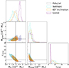 |
Fig. 6. One-and two-dimensional PDF distribution of the Mvir, M*, and cvir for the Fiducial model compared to the model variations discussed in Sect. 4.3. The PDF distributions for each model are shown in different colors: black for the Fiducial model, cyan for the “Isotropic model”, orange for the “60° inclination model”, and fuchsia for the “cored” model. The darker and lighter colors represent the 1 and 2-σ confidence intervals, respectively, for each model. The median value for the Fiducial model are shown in dashed black lines, and they are listed in Table 3 for the rest of the models. |
4.3.2. Radially varying anisotropy
Here we briefly explore whether the assumption of radially constant anisotropy for each tracer is meaningfully affecting our results. We fix the gravitational potential parameters to the values of the Fiducial model and then run single tracer fits, but replacing a single value of β with four logarithmically spaced radial ranges where it can take on different values in each region. We find no statistically significant evidence for a radial gradient in β for any of the tracer populations, indicating the assumption of a radially constant velocity anisotropy for each tracer is reasonable, at least for this dataset.
4.3.3. Varying inclination
In this subsection we study the effect of the assumed inclination in our dynamical models. As mentioned in Sect. 3, previous studies suggest the inclination of NGC 5128 is more likely edge-on, and in particular that face-on orientations are disfavored (Hui et al. 1995; Peng et al. 2004a).
Here we compare our edge-on (90°) model to one where the assumed inclination is instead the median value for a random distribution: 60°. The other model assumptions are identical to those of the Fiducial model. The resulting Mvir, cvir, and M* are shown in Fig. 6, and listed in Table 3.
The model with an inclination of 60° produces results consistent with the Fiducial model to within 1σ for all parameters, with a slightly higher concentration and a slightly lower (about 15% lower) virial mass.
4.3.4. A cored halo
For our Fiducial model we have assumed a standard cuspy NFW profile, corresponding to γ = η = 1 in Eq. (4). While giant elliptical galaxies tend to have dark matter profiles well-fit by a standard NFW profile (e.g., Grillo 2012), here we briefly consider the sensitivity our results to the assumed halo profile.
As a comparison “cored” model, we assume γ = 0 and η = 2 in Eq. (4), producing a central core rather than a cusp. All other model parameters are the same.
The differences in the fitted parameters between the cored and Fiducial are generally as one would expect: Mvir is essentially identical, being set by the data at larger radii, while the concentration is lower (cvir = 3.3 ± 0.4) due to the lesser central dark matter density. This forces the stellar mass-to-light ratio an implausibly high value ΥK = 2.3 ± 0.1 to match the inner kinematics, compensating for the lower dark matter density. This is in strong tension with our prior on ΥK (1.08 ± 0.30), and is higher than the mass-to-light ratio for stellar population models at any age and metallicity (e.g., Bruzual & Charlot 2003). This tension with stellar populations models disfavors the cored model relative to the standard NFW profile where we get mass-to-light ratios in agreement with stellar population expectations (see Sect. 4.1.2).
4.4. Conclusions
Our main conclusions from this section are:
– The best fit parameters of our Fiducial NFW model provides a good fit to nearly all the data, potentially with the exception of a subset of the PNe.
– The results are insensitive to modest variations in the tracer population used.
– The results are also relatively insensitive to modest variations in model assumptions about anisotropy or inclination, and such variations are not inconsistent with the data. However, a cored dark matter halo is disfavored, due to its unrealistic high stellar mass-to-light ratio (see discussion in Sect. 4.3.4).
Again, we summarize our mass modeling results in Table 3. We next compare our results with previous mass and mass profile measurements of NGC 5128.
5. Comparisons to previous NGC 5128 total mass and halo estimates
5.1. Comparison to enclosed mass estimates
Many previous estimates exist of the enclosed gravitational mass of NGC 5128 at a range of radii. These estimates are summarized in the left panel of Fig. 7 and compared to our new dynamical modeling.
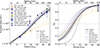 |
Fig. 7. Left: enclosed mass for the fiducial model as a function of galactocentric radius compared to literature measurements and different dynamical models from this work. The solid lines represent the median enclosed mass for each dynamical model based on 150 randomly selected walkers, while the shaded region represents the 1-σ uncertainty for the fiducial model. The symbols show the different NGC 5128 literature enclosed mass measurements (Hui et al. 1995; Mathieu et al. 1996; Kraft et al. 2003; Peng et al. 2004a; Woodley et al. 2007, 2010; Karachentsev et al. 2007; Hughes et al. 2023; Müller et al. 2022), as well as the lower limit from Pearson et al. (2022). We have colored the symbols according to the kinematic tracer used to inferred the total enclosed mass, with the colors representing the same tracer as in Fig. 1. Right: dark matter fraction (fDM) comparison for all the different dynamical models of this work. Lines are colored the same as in the left panel. The vertical lines show the virial radius for each dynamical model. |
We find good agreement between the results of our Fiducial model and the enclosed mass at smaller galactocentric radius (∼16 kpc) from the modeling of the galaxy’s interstellar X-ray emission by Kraft et al. (2003). Our Fiducial model also agrees with the enclosed mass at ∼27 kpc found by Hui et al. (1995) using a spherical and isotropic approximation of the Jeans equation to model the PNe distribution. For a detailed comparison of masses derived from X-ray observations and those from PNe and GCs at small galactocentric radii (< 55 kpc), see also Samurović (2006).
At larger radii, we find that our models have systematically lower masses than previous mass estimates made using only GCs or dwarfs as tracers (Woodley et al. 2007, 2010; Karachentsev et al. 2007; Alabi et al. 2017; Hughes et al. 2023). These previous works adopted relatively simpler dynamical models than the one presented here, using the “tracer mass estimator” (TME; Evans et al. 2003; Watkins et al. 2010) to calculate the pressure supported mass and used the spherical part of the Jeans equation to calculate the rotationally supported mass. This assumes a spherical and isotropic distribution of the kinematic tracers, which, depending on the tracer anisotropy, may underestimate or overestimate the enclosed mass (see discussion in Alabi et al. 2016). This could explain also why our isotropic GC-only model is in better agreement with their results. Using the same assumptions and method Bílek et al. (2019) derived a virial halo mass of Mvir = 1013.9 − 14.2 M⊙, which is more than an order bigger than our Mvir, maybe due to their much higher NFW scale density (see Sect. 5.2). The halo mass of our Fiducial model at a contrast density of 200 ( M⊙) is in agreement with the halo mass of
  M⊙ derived by Alabi et al. (2017) based also on the kinematics of GCs using the same method described above. The M200 = 5.3 ± 3.5 × 10¹² M⊙ estimates based on kinematics of dwarf satellite galaxies by Müller et al. (2022) using the rotational part of the Jeans equation is larger than what we find for our Fiducial model, but they both agrees within uncertainties. The M200 of our Fiducial model is also smaller than the limit of M200 > 4.7 × 10¹² M⊙ derived from modeling of the stellar stream from the disrupted dwarf satellite Dw3 by Pearson et al. (2022). However, we note that their DM halo model was fixed to match the enclosed mass at smaller galactocentric radius of Woodley et al. (2010).
The agreement between our fiducial model and the enclosed masses from PNe at larger radii is more mixed. Our models match the enclosed mass at ∼86 kpc from Peng et al. (2004a) derived using the tracer mass estimator method from Evans et al. (2003) assuming a spherical and isotropic distribution for the PNe, but we find higher masses than Woodley et al. (2007) (also done using the tracer mass estimator method), and by Mathieu et al. (1996; assuming also a spherical and isotropic distribution for the PNe). These comparisons are consistent with the interpretation that our best-fit Fiducial model represents a statistical compromise among these tracers.
5.2. Comparison to previous dark matter profile fits
Four previous works, Peng et al. (2004a), Alabi et al. (2017), Bílek et al. (2019) and Pearson et al. (2022), have estimated parameters for a standard NFW profile for NGC 5128. Peng et al. (2004a) fitted PNe using an isotropic spherically symmetric Jeans model, obtaining an NFW scale density of log(ρs)= − 2.0 and scale radius of rs = 14.4 kpc (no uncertainties reported). There is no mention of the M200 for the NFW profile in Peng et al. (2004a), only c200 = 12. However, we can estimate an M200 = 6.32 × 10¹¹ M⊙ based on their rs and ρs. These values are all inconsistent with those from our fiducial model, producing a more centrally concentrated and much lower mass halo. For comparison to these results we run an isotropic (βPNe = 0.0) MCMC with only the PNe as kinematic tracers, but otherwise with the same assumptions as in our fiducial model. For this isotropic PNe-only model, we find a scale density  and scale radius of
  kpc, in very good agreement with the values found by Peng et al. (2004a). This comparison illustrates both the value of large-radius tracers for estimating the total halo mass, and, to a lesser degree, the effect of anisotropy on the fits.
Pearson et al. (2022) used the stellar stream of the dwarf satellite galaxy Dw3 (at a projected radius of ∼80 kpc) to estimate a lower limit of the dark matter halo mass of NGC 5128 of M200 > 4.7 × 10¹² M⊙, with an assumed c200 = 8.6 and stellar mass-to-light ratio of ΥK = 0.7. These values correspond to a more centrally concentrated, massive dark matter halo than our fiducial model. The dynamical modeling of Dw3 done by Pearson et al. (2022) was tuned to reproduce the enclosed mass at 40 kpc found by Woodley et al. (2010) based on GC kinematics.
Of the models fit in the previous section, the one which is most comparable to this is the anisotropic “GC only” model (Sect. 4.2). For this model, we find  M⊙, broadly consistent with the M200 lower limit from Pearson et al. (2022). They conclude that the morphology and central radial velocity for a single stream is insufficient to precisely determine halo parameters; revisiting this stream fitting with the updated tracer constraints now available would be worthwhile.
Our fiducial model agrees with the halo concentration of cvir = 4 − 5 derived by Bílek et al. (2019) for NGC 5128 from the Jeans modeling of its GC kinematics (among other early-type galaxies), which is lower than expected from concentration-mass relations (see Sect. 6.2). The halo concentration reported in Alabi et al. (2017) for NGC 5128 c200 = 8.9 ± 2.0 is higher than what we find here. While Alabi et al. (2017) do not explicitly provide a scale radius for NGC 5128 we can derive it from their c200 and M200 values, giving a rs = 39.1 ± 7.9 kpc, which is smaller than the scale radius of our fiducial model, but they roughly agree within uncertainties (see Table 2). The scale scale density and radius found in Bílek et al. (2019) for NGC 5128 (log(ρs)=5.6 − 5.8 and log(rs)=2.4 − 2.5) are both higher than our values.
6. Discussion
6.1. Dark matter fractions
Our dynamical model fitting in Sect. 4 show the need for large amounts of dark matter to explain the dynamics of the GCs, PNe, and dwarf satellite galaxies in NGC 5128, with a best-fit virial halo mass of  and a stellar mass of ∼0.2 × 10¹² M⊙. Hence globally, the stellar mass fraction of the galaxy is found to be ∼4% (formally
  ).
).
The stellar mass–halo mass relation has been measured for galaxies in a variety of ways, including abundance matching (e.g., Moster et al. 2010), weak lensing (e.g., Leauthaud et al. 2012), and from clustering analysis (e.g., Zheng et al. 2007). A recent compilation of stellar mass–halo mass relations from Behroozi et al. (2019) shows that at NGC 5128’s measured virial mass, the expected stellar mass fraction is 1–3%. The higher end of that range is consistent with the measured stellar mass fraction within its uncertainty, while the lower end is less consistent, suggesting the possibility that NGC 5128 was more efficient than the average galaxy of this virial mass at transforming baryons into stars. This is in agreement with the general trend of higher than expected stellar mass values in the sample of early-type galaxies modeled by Bílek et al. (2019); however, our results disagree with their results on NGC 5128, as we find more than order of magnitude lower halo mass than their study.
Since observational measurements encompassing a large fraction of the virial radius are challenging, many observational studies have focused instead on quantifying the fraction of dark matter in the inner portions of galaxies, often measured at notional comparison radii of 1 and 5Reff. For the total mass-to-light ratio (stellar + dark matter) we find a value of ΥK(< 1Reff)=1.3 at 1Reff. This translates to Υr(< 1Reff)=4.6 (assuming a r − Ks = 2.6); this is identical to the mean value of Υr(< 1Reff) in ATLAS3D galaxies (Cappellari et al. 2013a). For the dark matter fraction (fDM) in NGC 5128 within 1Reff we find fDM = 0.11 ± 0.04 for our fiducial model. Previous dynamical modeling results for other early-type galaxies (Cappellari et al. 2011), along with spiral and S0 galaxies (Williams et al. 2009), show this to be a typical value, with most galaxies in these samples having fDM < 0.2 at 1Reff. Individual galaxy measurements for the giant elliptical M87 and NGC 5846, more comparable to the approach we use for NGC 5128, also find fDM ∼ 0.1 within 1Reff (Zhu et al. 2014, 2016). However, theoretical models (Lovell et al. 2018) and other dynamical and lensing results (Barnabè et al. 2011; Tortora et al. 2012) suggest higher dark matter fractions within 1Reff. This is a tension previously recognized. It could be due to inconsistencies in how sizes are measured for real galaxies compared to those in simulations, uncertainty about the initial mass function in early-type galaxies (additional discussion in e.g., van Dokkum et al. 2017; Bílek et al. 2019), or perhaps due to true differences between the inner dark matter distribution in observed galaxies compared to simulations (see additional discussion in Lovell et al. 2018).
At larger radii, within 5Reff, we find fDM = 0.52 ± 0.08. Previous measurements using tracer-mass estimator methods on large GC samples from the SLUGGS project (Alabi et al. 2017) find a wide range of dark matter fractions within 5Reff from fDM of 0.1 to 0.95, with most higher than NGC 5128. Jeans modeling of early-type GCs by Bílek et al. (2019) also find generally high dark matter fractions, with their results for NGC 5128 (∼90%) being higher than those found here. Simulations generally find less scatter in fDM at these larger radii among galaxies than do observations, but do not agree on the actual value of fDM. For example, Wu et al. (2014) find ∼0.5 for fDM for galaxies in the stellar mass range of NGC 5128, while more recent results from Remus et al. (2017) and Lovell et al. (2018) suggest much higher fDM ≳ 0.7 with minimal scatter. We note that the methodology of existing observational measurements varies significantly, with many studies using basic spherical isotropic dynamical models with limited radial tracer coverage, and only a handful of previous estimates are based on Jeans modeling out to large radii as we present here.
6.2. Concentration–mass relation
Numerical simulations show that the structural properties of dark matter halos change as a function of mass, with higher mass halos becoming less concentrated, as halo density is correlated with the density of the universe at the time of formation (e.g., Navarro et al. 1997; Bullock et al. 2001). The relation between halo mass and concentration is thus an important tracer of the formation history of galaxy halos.
As a prior on the NFW dark matter component of our NGC 5128 mass model, we adopted the concentration–mass (cvir − Mvir) relation of Bullock et al. (2001). This prior of cvir = 14.0 ± 5.6 was estimated based on a previous NGC 5128 mass measurement (Woodley et al. 2007). The actual estimated value of cvir for our fiducial model is cvir=5.6 with a
  . That our best-fit concentration is in the tail of the prior indicates the data quite strongly favor the measured low concentration. Our low concentration is consistent with the values derived by Bílek et al. (2019) for NGC 5128, and more broadly they find a majority of modeled early-type galaxies fall below the halo-mass – concentration relation of Diemer & Kravtsov (2015).
The measured value is in somewhat better agreement with the more recent concentration–mass relations of Muñoz-Cuartas et al. (2011), Dutton & Macciò (2014), and Diemer & Kravtsov (2015), who find mean values of cvir between 8.3 and 9.1 at our virial mass. While our fiducial concentration value is still nominally lower than these predictions, the simulations exhibit significant halo to halo scatter in cvir − Mvir, of order ∼30%. Hence the overall conclusion is that NGC 5128’s inferred dark matter halo is consistent with the distribution of halo properties at this virial mass observed in cosmological simulations. A much larger set of measured halo concentrations for massive ellipticals would be necessary to more carefully compare simulations to observations.
6.3. Halo mass–NGC relation
A number of papers have demonstrated a relationship between the number of GCs in a galaxy (NGC) and its total (including dark matter) mass, which is apparently linear over a large range in halo masses (e.g., Harris et al. 2017; Burkert & Forbes 2020). It is notable that the claimed scatter in this relation is small (< 0.3 dex), which if true would make the counting of GCs one of the most reliable methods to estimate halo masses.
Since NGC 5128 has both a good estimate of its total GC population (NGC = 1450 ± 160; Hughes et al. 2021) and total mass from the present work ( , see Sect. 4.1.1), it presents a compelling test of this relation. We use the two most recent derived versions of the relation, from Harris et al. (2017) and Burkert & Forbes (2020). For the former, the predicted mass from the measured NGC is ∼1.6 × 10¹³ M⊙, with an uncertainty of about a factor of 2 from the stated scatter in the relation. The offset of NGC 5128 from the relation is about 0.54 dex, or nearly 2σ on the low end. For the Burkert & Forbes (2020) relation, the inferred halo mass is lower, about 7×10¹² M⊙, which is higher than but in less tension than our NGC 5128 mass measurement.
As we discussed above for the measurement of halo concentration, it is impossible to reach a firm conclusion about variance in one of these relations from a single measurement. Nonetheless, given the small number of galaxies for which there are robust measurements of both their virial masses and GC systems, revisiting the scatter in the NGC–total mass relation should be a priority once more virial mass estimates are available.
6.4. The mass of NGC 5128 in context
NGC 5128 is one of the more massive galaxies within ∼5 Mpc, making it an important benchmark system for connecting its stellar and dark matter halo properties to expectations from the ΛCDM model and other prominent, nearby galaxies.
Within the Local Group, the masses of the Milky Way and M31 have been the subject of many studies. For the Milky Way, astrometric data from the Gaia mission has provided critical tangential velocities for many mass tracers (satellites galaxies, GCs and halo stars; see e.g., Callingham et al. 2019; Eadie & Jurić 2019; Watkins et al. 2019; Li et al. 2020; Deason et al. 2021), improving agreement between recent studies, most of which point to total masses around 1–1.5 × 10¹² M⊙ (see Wang et al. 2020b, for a recent review). This mass of the Milky Way is similar to mass estimates of other nearby, massive spiral galaxies; Mvir, M83 ≈ 0.9 × 10¹² M⊙ (Karachentsev et al. 2007); Mvir, M81 ≈ 1 × 10¹² M⊙ (Karachentsev & Kashibadze 2006). This places NGC 5128 at about three to four times more massive than the Milky Way and other nearby spirals.
In M31, modern measurements have yielded virial mass values in the range Mvir,M31 = 0.5–3.5 × 10¹² M⊙, including satellite galaxy (Watkins et al. 2010; Hayashi & Chiba 2014), globular cluster (e.g., Veljanoski et al. 2013) and stellar stream (Fardal et al. 2013; Dey et al. 2023) kinematic measurements; see the recent compilation of Patel & Mandel (2023). In that same work, Patel & Mandel (2023) combine proper motion measurements of four M31 satellites and cosmological simulations to infer Mvir, M31 = 2.85 × 10¹² M⊙. This value is within a factor of ∼1.5 of the NGC 5128 virial mass, and the uncertainties of the two measurements overlap. Those authors also note that M31 is on the upper end of expectations for the stellar mass-halo mass relation, as we have seen for NGC 5128 in Sect. 6.1. Future measurements are necessary to confirm this most recent, relatively high mass for M31. Nonetheless, it is plausible that M31 and NGC 5128 have similar masses.
The M200 halo mass of NGC 5128 is comparable to other nearby elliptical galaxies, such as NGC 1023, NGC 4473 and NGC 4494 from Alabi et al. (2017), which also have similar stellar mass5. NGC 1023 and NGC 4494 are both the central galaxy in their group (NGC 4473 is classified as a group member) and have lower than expected halo concentration. From the elliptical galaxies sample of Bílek et al. (2019), NGC 1400 and NGC 2768 have similar virial halo mass to NGC 5128, and are also central galaxies in their group. This suggests that NGC 1023, NGC 4494, NGC 1400, NGC 2768 and NGC 5128 may have formed in a similar way. However, we note that the halo mass for NGC 2768 found in Alabi et al. (2017) is about one order of magnitude bigger than Bílek et al. (2019).
Kinematic measurements out to large radii (≳50–100 kpc) using GCs, PNe and satellite galaxies is feasible for more galaxies in the nearby universe. Existing studies of large samples of galaxies have used single kinematic tracers (Alabi et al. 2017; Bílek et al. 2019). A systematic data set that pursued this goal with multiple tracers would be valuable for constraining the virial masses and mass profiles of the nearest massive galaxy halos in a consistent way, allowing for further intercomparisons and comparisons with ΛCDM.
7. Summary
We used the discrete Jeans anistoropic model CJAM (Watkins et al. 2013) to estimate the halo parameters of NGC 5128 using its GCs, PNe, and dwarf satellite galaxies as kinematic tracers out to a radius of 250 kpc, with the tracer anisotropies and stellar mass-to-light ratio fit as free parameters.
Our fiducial model fit has a dark matter halo virial mass of  , a concentration of
  , and a corresponding virial radius of
  kpc. This halo constitutes only ∼10% of the total mass at 1Reff but ∼51% at 5Reff. This model fits nearly all the data, with the exception of a subset of the PNe that are potentially not in virial equilibrium, and the derived halo parameters are relatively insensitive to modest variations in the tracer anisotropies and system inclination.
NGC 5128 appears to sit “low” on the mean stellar mass–halo mass and GC mass–halo mass relations, which both predict a halo virial mass closer to Mvir ∼ 1013 M⊙. No general statements about these relations can be made with a single galaxy, but our analysis highlights the value of comprehensive dynamical modeling of nearby galaxies, and the importance of using multiple tracers to allow cross-checks for model robustness.
This calculation is based on the K-band magnitude from Jarrett et al. (2003), combined with the available B and V-band colors from NED (which have similar radial coverage).
From the NASA/IPAC Extragalactic Database (NED).
They derived a stellar mass for NGC 5128 of M* = 8.7 × 10¹⁰ M⊙ because they assume a ΥK = 1 (also for all the galaxies in their sample), which is lower than our best-fit  .
.
Acknowledgments
Dedicated to the memory of Ruth Neira Johnston (1953–2024). We acknowledge the useful comments of the referee, which improved the presentation of this work. Work by A.D. and A.C.S. has been supported by NSF AST-1813609. A.K.H. and D.J.S. acknowledge support from NSF grants AST-1821967 and 1813708. N.C. acknowledges support by NSF grant AST-1812461. J.S. acknowledges support from NSF grants AST-1514763 and AST-1812856 and the Packard Foundation. Support for S.P. work was provided by NASA through the NASA Hubble Fellowship grant #HST-HF2-51466.001-A awarded by the Space Telescope Science Institute, which is operated by the Association of Universities for Research in Astronomy, Incorporated, under NASA contract NAS5-26555. This paper made use of the MGE fitting method and software by Cappellari (2002) and JAM modeling method of Cappellari (2008), as well as discrete dynamical model extension to JAM by Watkins et al. (2013), and the astropy package (Astropy Collaboration 2013).
References
- Alabi, A. B., Forbes, D. A., Romanowsky, A. J., et al. 2016, MNRAS, 460, 3838 [Google Scholar]
- Alabi, A. B., Forbes, D. A., Romanowsky, A. J., et al. 2017, MNRAS, 468, 3949 [Google Scholar]
- Astropy Collaboration (Robitaille, T. P., et al.) 2013, A&A, 558, A33 [NASA ADS] [CrossRef] [EDP Sciences] [Google Scholar]
- Auger, M. W., Treu, T., Bolton, A. S., et al. 2010, ApJ, 724, 511 [NASA ADS] [CrossRef] [Google Scholar]
- Barnabè, M., Czoske, O., Koopmans, L. V. E., Treu, T., & Bolton, A. S. 2011, MNRAS, 415, 2215 [Google Scholar]
- Beasley, M. A., Bridges, T., Peng, E., et al. 2008, MNRAS, 386, 1443 [NASA ADS] [CrossRef] [Google Scholar]
- Behroozi, P., Wechsler, R. H., Hearin, A. P., & Conroy, C. 2019, MNRAS, 488, 3143 [NASA ADS] [CrossRef] [Google Scholar]
- Bílek, M., Samurović, S., & Renaud, F. 2019, A&A, 625, A32 [Google Scholar]
- Binney, J., & Mamon, G. A. 1982, MNRAS, 200, 361 [Google Scholar]
- Bosma, A. 1978, PhD Thesis, University of Groningen, The Netherlands [Google Scholar]
- Bosma, A. 1981, AJ, 86, 1791 [NASA ADS] [CrossRef] [Google Scholar]
- Brodie, J. P., & Strader, J. 2006, ARA&A, 44, 193 [Google Scholar]
- Brodie, J. P., Romanowsky, A. J., Strader, J., et al. 2014, ApJ, 796, 52 [Google Scholar]
- Bruzual, G., & Charlot, S. 2003, MNRAS, 344, 1000 [NASA ADS] [CrossRef] [Google Scholar]
- Bullock, J. S., Kolatt, T. S., Sigad, Y., et al. 2001, MNRAS, 321, 559 [Google Scholar]
- Burkert, A., & Forbes, D. A. 2020, AJ, 159, 56 [Google Scholar]
- Callingham, T. M., Cautun, M., Deason, A. J., et al. 2019, MNRAS, 484, 5453 [Google Scholar]
- Cappellari, M. 2002, MNRAS, 333, 400 [NASA ADS] [CrossRef] [Google Scholar]
- Cappellari, M. 2008, MNRAS, 390, 71 [NASA ADS] [CrossRef] [Google Scholar]
- Cappellari, M., Neumayer, N., Reunanen, J., et al. 2009, MNRAS, 394, 660 [NASA ADS] [CrossRef] [Google Scholar]
- Cappellari, M., Emsellem, E., Krajnović, D., et al. 2011, MNRAS, 413, 813 [Google Scholar]
- Cappellari, M., McDermid, R. M., Alatalo, K., et al. 2013a, MNRAS, 432, 1862 [NASA ADS] [CrossRef] [Google Scholar]
- Cappellari, M., Scott, N., Alatalo, K., et al. 2013b, MNRAS, 432, 1709 [Google Scholar]
- Carlsten, S. G., Greene, J. E., Peter, A. H. G., Greco, J. P., & Beaton, R. L. 2020, ApJ, 902, 124 [NASA ADS] [CrossRef] [Google Scholar]
- Coccato, L., Arnaboldi, M., & Gerhard, O. 2013, MNRAS, 436, 1322 [Google Scholar]
- Crnojević, D., Sand, D. J., Bennet, P., et al. 2019, ApJ, 872, 80 [Google Scholar]
- Deason, A. J., Erkal, D., Belokurov, V., et al. 2021, MNRAS, 501, 5964 [Google Scholar]
- Dey, A., Najita, J. R., Koposov, S. E., et al. 2023, ApJ, 944, 1 [NASA ADS] [CrossRef] [Google Scholar]
- Diemer, B., & Kravtsov, A. V. 2015, ApJ, 799, 108 [Google Scholar]
- Doliva-Dolinsky, A., Martin, N. F., Yuan, Z., et al. 2023, ApJ, 952, 72 [CrossRef] [Google Scholar]
- Dufour, R. J., van den Bergh, S., Harvel, C. A., et al. 1979, AJ, 84, 284 [NASA ADS] [CrossRef] [Google Scholar]
- Dumont, A., Seth, A. C., Strader, J., et al. 2022, ApJ, 929, 147 [NASA ADS] [CrossRef] [Google Scholar]
- Dutton, A. A., & Macciò, A. V. 2014, MNRAS, 441, 3359 [Google Scholar]
- Eadie, G., & Jurić, M. 2019, ApJ, 875, 159 [NASA ADS] [CrossRef] [Google Scholar]
- Erkal, D., Belokurov, V., Laporte, C. F. P., et al. 2019, MNRAS, 487, 2685 [Google Scholar]
- Evans, N. W., Wilkinson, M. I., Perrett, K. M., & Bridges, T. J. 2003, ApJ, 583, 752 [NASA ADS] [CrossRef] [Google Scholar]
- Fahrion, K., Müller, O., Rejkuba, M., et al. 2020, A&A, 634, A53 [NASA ADS] [CrossRef] [EDP Sciences] [Google Scholar]
- Fardal, M. A., Weinberg, M. D., Babul, A., et al. 2013, MNRAS, 434, 2779 [Google Scholar]
- Forbes, D. A., Alabi, A., Romanowsky, A. J., et al. 2017, MNRAS, 464, L26 [NASA ADS] [CrossRef] [Google Scholar]
- Foreman-Mackey, D., Hogg, D. W., Lang, D., & Goodman, J. 2013, PASP, 125, 306 [Google Scholar]
- Georgiev, I. Y., Puzia, T. H., Hilker, M., & Goudfrooij, P. 2009, MNRAS, 392, 879 [NASA ADS] [CrossRef] [Google Scholar]
- Graham, J. A., & Phillips, M. M. 1980, ApJ, 239, L97 [NASA ADS] [CrossRef] [Google Scholar]
- Grillo, C. 2012, ApJ, 747, L15 [Google Scholar]
- Häring-Neumayer, N., Cappellari, M., Rix, H. W., et al. 2006, ApJ, 643, 226 [CrossRef] [Google Scholar]
- Harris, G. L. H. 2010, PASA, 27, 475 [NASA ADS] [CrossRef] [Google Scholar]
- Harris, G. L. H., Harris, W. E., & Geisler, D. 2004, AJ, 128, 723 [NASA ADS] [CrossRef] [Google Scholar]
- Harris, W. E., Harris, G. L. H., Holland, S. T., & McLaughlin, D. E. 2002, AJ, 124, 1435 [NASA ADS] [CrossRef] [Google Scholar]
- Harris, W. E., Blakeslee, J. P., & Harris, G. L. H. 2017, ApJ, 836, 67 [Google Scholar]
- Hartke, J., Arnaboldi, M., Gerhard, O., et al. 2018, A&A, 616, A123 [NASA ADS] [CrossRef] [EDP Sciences] [Google Scholar]
- Hayashi, K., & Chiba, M. 2014, ApJ, 789, 62 [Google Scholar]
- Hesser, J. E., Harris, H. C., & Harris, G. L. H. 1986, ApJ, 303, L51 [NASA ADS] [CrossRef] [Google Scholar]
- Hughes, A. K., Sand, D. J., Seth, A., et al. 2021, ApJ, 914, 16 [NASA ADS] [CrossRef] [Google Scholar]
- Hughes, A. K., Sand, D. J., Seth, A., et al. 2023, ApJ, 947, 34 [NASA ADS] [CrossRef] [Google Scholar]
- Hui, X., Ford, H. C., Freeman, K. C., & Dopita, M. A. 1995, ApJ, 449, 592 [Google Scholar]
- Israel, F. P. 1998, A&A Rev., 8, 237 [Google Scholar]
- Jarrett, T. H., Chester, T., Cutri, R., Schneider, S. E., & Huchra, J. P. 2003, AJ, 125, 525 [Google Scholar]
- Karachentsev, I. D., & Kashibadze, O. G. 2006, Astrophysics, 49, 3 [NASA ADS] [CrossRef] [Google Scholar]
- Karachentsev, I. D., Sharina, M. E., Dolphin, A. E., et al. 2002, A&A, 385, 21 [CrossRef] [EDP Sciences] [Google Scholar]
- Karachentsev, I. D., Tully, R. B., Dolphin, A., et al. 2007, AJ, 133, 504 [NASA ADS] [CrossRef] [Google Scholar]
- Kim, D.-W., & Fabbiano, G. 2013, ApJ, 776, 116 [NASA ADS] [CrossRef] [Google Scholar]
- Kraft, R. P., Vázquez, S. E., Forman, W. R., et al. 2003, ApJ, 592, 129 [NASA ADS] [CrossRef] [Google Scholar]
- Leauthaud, A., Tinker, J., Bundy, K., et al. 2012, ApJ, 744, 159 [Google Scholar]
- Li, H., Li, R., Mao, S., et al. 2016, MNRAS, 455, 3680 [CrossRef] [Google Scholar]
- Li, Z.-Z., Qian, Y.-Z., Han, J., et al. 2020, ApJ, 894, 10 [Google Scholar]
- Lilleengen, S., Petersen, M. S., Erkal, D., et al. 2023, MNRAS, 518, 774 [Google Scholar]
- Lovell, M. R., Pillepich, A., Genel, S., et al. 2018, MNRAS, 481, 1950 [Google Scholar]
- Marigo, P., Girardi, L., Bressan, A., et al. 2017, ApJ, 835, 77 [Google Scholar]
- Martini, P., & Ho, L. C. 2004, ApJ, 610, 233 [NASA ADS] [CrossRef] [Google Scholar]
- Martinsson, T. P. K., Verheijen, M. A. W., Westfall, K. B., et al. 2013, A&A, 557, A131 [NASA ADS] [CrossRef] [EDP Sciences] [Google Scholar]
- Mathieu, A., Dejonghe, H., & Hui, X. 1996, A&A, 309, 30 [NASA ADS] [Google Scholar]
- Moster, B. P., Somerville, R. S., Maulbetsch, C., et al. 2010, ApJ, 710, 903 [Google Scholar]
- Muñoz-Cuartas, J. C., Macciò, A. V., Gottlöber, S., & Dutton, A. A. 2011, MNRAS, 411, 584 [Google Scholar]
- Müller, O., Pawlowski, M. S., Lelli, F., et al. 2021, A&A, 645, L5 [NASA ADS] [CrossRef] [EDP Sciences] [Google Scholar]
- Müller, O., Lelli, F., Famaey, B., et al. 2022, A&A, 662, A57 [NASA ADS] [CrossRef] [EDP Sciences] [Google Scholar]
- Napolitano, N. R., Pota, V., Romanowsky, A. J., et al. 2014, MNRAS, 439, 659 [NASA ADS] [CrossRef] [Google Scholar]
- Navarro, J. F., Frenk, C. S., & White, S. D. M. 1996, ApJ, 462, 563 [Google Scholar]
- Navarro, J. F., Frenk, C. S., & White, S. D. M. 1997, ApJ, 490, 493 [Google Scholar]
- Nibauer, J., Bonaca, A., & Johnston, K. V. 2023, ApJ, 954, 195 [NASA ADS] [CrossRef] [Google Scholar]
- Patel, E., & Mandel, K. S. 2023, ApJ, 948, 104 [NASA ADS] [CrossRef] [Google Scholar]
- Pawlowski, M. S., Oria, P.-A., Taibi, S., Famaey, B., & Ibata, R. 2022, ApJ, 932, 70 [NASA ADS] [CrossRef] [Google Scholar]
- Pearson, S., Price-Whelan, A. M., Hogg, D. W., et al. 2022, ApJ, 941, 19 [NASA ADS] [CrossRef] [Google Scholar]
- Peng, E. W., Ford, H. C., & Freeman, K. C. 2004a, ApJS, 150, 367 [NASA ADS] [CrossRef] [Google Scholar]
- Peng, E. W., Ford, H. C., & Freeman, K. C. 2004b, ApJ, 602, 705 [NASA ADS] [CrossRef] [Google Scholar]
- Planck Collaboration XIII. 2016, A&A, 594, A13 [NASA ADS] [CrossRef] [EDP Sciences] [Google Scholar]
- Planck Collaboration VI. 2020, A&A, 641, A6 [NASA ADS] [CrossRef] [EDP Sciences] [Google Scholar]
- Rejkuba, M., Dubath, P., Minniti, D., & Meylan, G. 2007, A&A, 469, 147 [NASA ADS] [CrossRef] [EDP Sciences] [Google Scholar]
- Rejkuba, M., Harris, W. E., Greggio, L., & Harris, G. L. H. 2011, A&A, 526, A123 [NASA ADS] [CrossRef] [EDP Sciences] [Google Scholar]
- Rejkuba, M., Harris, W. E., Greggio, L., Crnojević, D., & Harris, G. L. H. 2022, A&A, 657, A41 [NASA ADS] [CrossRef] [EDP Sciences] [Google Scholar]
- Remus, R.-S., Dolag, K., Naab, T., et al. 2017, MNRAS, 464, 3742 [Google Scholar]
- Richtler, T., Hilker, M., Kumar, B., et al. 2014, A&A, 569, A41 [NASA ADS] [CrossRef] [EDP Sciences] [Google Scholar]
- Rubin, V. C., Ford, W. K., Jr., & Thonnard, N., 1978, ApJ, 225, L107 [NASA ADS] [CrossRef] [Google Scholar]
- Samurović, S. 2006, Serb. Astron. J., 173, 35 [CrossRef] [Google Scholar]
- Shipp, N., Erkal, D., Drlica-Wagner, A., et al. 2021, ApJ, 923, 149 [NASA ADS] [CrossRef] [Google Scholar]
- Silge, J. D., Gebhardt, K., Bergmann, M., & Richstone, D. 2005, AJ, 130, 406 [NASA ADS] [CrossRef] [Google Scholar]
- Sofue, Y., & Rubin, V. 2001, ARA&A, 39, 137 [NASA ADS] [CrossRef] [Google Scholar]
- Sofue, Y., Tutui, Y., Honma, M., et al. 1999, ApJ, 523, 136 [NASA ADS] [CrossRef] [Google Scholar]
- Taylor, M. A., Puzia, T. H., Harris, G. L., et al. 2010, ApJ, 712, 1191 [NASA ADS] [CrossRef] [Google Scholar]
- Taylor, M. A., Puzia, T. H., Gomez, M., & Woodley, K. A. 2015, ApJ, 805, 65 [NASA ADS] [CrossRef] [Google Scholar]
- Tortora, C., La Barbera, F., Napolitano, N. R., de Carvalho, R. R., & Romanowsky, A. J. 2012, MNRAS, 425, 577 [NASA ADS] [CrossRef] [Google Scholar]
- van den Bergh, S., Hesser, J. E., & Harris, G. L. H. 1981, AJ, 86, 24 [NASA ADS] [CrossRef] [Google Scholar]
- van Dokkum, P., Conroy, C., Villaume, A., Brodie, J., & Romanowsky, A. J. 2017, ApJ, 841, 68 [Google Scholar]
- Veljanoski, J., Ferguson, A. M. N., Mackey, A. D., et al. 2013, ApJ, 768, L33 [NASA ADS] [CrossRef] [Google Scholar]
- Veršič, T., Rejkuba, M., & Arnaboldi, M. 2023, arXiv e-prints [arXiv:2305.09822] [Google Scholar]
- Voggel, K. T., Seth, A. C., Sand, D. J., et al. 2020, ApJ, 899, 140 [NASA ADS] [CrossRef] [Google Scholar]
- Walker, M. G., Mateo, M., Olszewski, E. W., Sen, B., & Woodroofe, M. 2009, AJ, 137, 3109 [NASA ADS] [CrossRef] [Google Scholar]
- Walsh, J. R., Rejkuba, M., & Walton, N. A. 2015, A&A, 574, A109 [NASA ADS] [CrossRef] [EDP Sciences] [Google Scholar]
- Wang, J., Hammer, F., Rejkuba, M., Crnojević, D., & Yang, Y. 2020a, MNRAS, 498, 2766 [NASA ADS] [CrossRef] [Google Scholar]
- Wang, W., Han, J., Cautun, M., Li, Z., & Ishigaki, M. N. 2020b, Sci. China Phys. Mech. Astron., 63 [Google Scholar]
- Watkins, L. L., Evans, N. W., & An, J. H. 2010, MNRAS, 406, 264 [Google Scholar]
- Watkins, L. L., van de Ven, G., den Brok, M., & van den Bosch, R. C. E. 2013, MNRAS, 436, 2598 [Google Scholar]
- Watkins, L. L., van der Marel, R. P., Sohn, S. T., & Evans, N. W. 2019, ApJ, 873, 118 [NASA ADS] [CrossRef] [Google Scholar]
- Wechsler, R. H., & Tinker, J. L. 2018, ARA&A, 56, 435 [NASA ADS] [CrossRef] [Google Scholar]
- Williams, M. J., Bureau, M., & Cappellari, M. 2009, MNRAS, 400, 1665 [NASA ADS] [CrossRef] [Google Scholar]
- Woodley, K. A., Harris, W. E., & Harris, G. L. H. 2005, AJ, 129, 2654 [NASA ADS] [CrossRef] [Google Scholar]
- Woodley, K. A., Harris, W. E., Beasley, M. A., et al. 2007, AJ, 134, 494 [NASA ADS] [CrossRef] [Google Scholar]
- Woodley, K. A., Gómez, M., Harris, W. E., Geisler, D., & Harris, G. L. H. 2010, AJ, 139, 1871 [NASA ADS] [CrossRef] [Google Scholar]
- Wu, X., Gerhard, O., Naab, T., et al. 2014, MNRAS, 438, 2701 [Google Scholar]
- Zhao, H. 1996, MNRAS, 278, 488 [Google Scholar]
- Zheng, Z., Coil, A. L., & Zehavi, I. 2007, ApJ, 667, 760 [Google Scholar]
- Zhu, L., Long, R. J., Mao, S., et al. 2014, ApJ, 792, 59 [CrossRef] [Google Scholar]
- Zhu, L., Romanowsky, A. J., van de Ven, G., et al. 2016, MNRAS, 462, 4001 [Google Scholar]
Appendix
Table A.1 lists the binned Vrms for all our kinematic tracers shown in Figure 4.
Tracer’s binned Vrms
All Tables
All Figures
|
Fig. 1. Radial distribution of the LOS velocity for the PNe (yellow), metal rich, and metal poor GCs (red and blue respectively), and the dwarf satellite galaxies (green) around NGC 5128. The LOS velocities are with respect to the systemic velocity of NGC 5128 of 540 km s−1 (Hughes et al. 2023). The solid black line shows the radial profile for the escape velocity for NGC 5128 derived from our best-fit mass model including dark matter presented in Sect. 4.1, while the dashed lines shows the escape velocity for just the stellar mass. The bottom panel is a histogram with the radial distribution for the PNe, GCs and dwarfs in the same colors as the top panel. |
| In the text | |
|
Fig. 2. Stellar surface brightness profile of NGC 5128. This figure shows a comparison between the best-fit MGE model for the surface brightness (red) with the 2MASS Large Galaxy Atlas surface brightness profile (blue) Jarrett et al. (2003), literature MGE model of NGC 5128 (dashed black line) by Häring-Neumayer et al. (2006), and the outer halo profiles in the V-band by Dufour et al. (1979) and Rejkuba et al. (2022) (green and yellow respectively), assuming a V − Ks = 3 mag. The blue horizontal dashed line represents the 2MASS surface brightness 1σ noise level used to derived the most inner part of the MGE model. The vertical bands show the radius at which we use the 2MASS K-band image, the de Vaucouleurs-Sérsic profile by Dufour et al. (1979) and Rejkuba et al. (2022) respectively to derive the MGE model shown in red. |
| In the text | |
|
Fig. 3. Top: MCMC post-burn distribution for the seven free parameter of the fiducial model. The histograms show their marginalized PDF, and the vertical blue lines show their best-fit value and their 1-σ error. The scatter plots show the two-dimensional PDF for the parameters colored by log-likelihood, with yellow colors indicating higher values. The red-dashed lines indicate each parameter’s best-fit value (median) location, and the black-dashed contours show their 1-σ and 2-σ error. Bottom: plots show the one and two-dimensional PDF distribution for Mvir, M* and cvir. Lines and contours in this plot are the same as in the left panel, but all are shown here in black. |
| In the text | |
|
Fig. 4. Comparison of observed Vrms radial profiles for the different kinematic tracers (outlined points) to predicted profiles from our best-fit fiducial dynamical model (colored rectangles). The colors represent the same tracers as in Fig. 1. This figure shows that the fiducial model does an excellent job of explaining the overall velocity distribution of our tracers. |
| In the text | |
|
Fig. 5. One-and two-dimensional PDF of Mvir, cvir, and M* of the fiducial model compared to the PDF inferred from single-tracer anisotropic models. The blue PDF represents the GC-only model, the yellow PDF the PNe-only model, and the green PDF the dwarfs-only model. We represent 1-σ and 2-σ confidence intervals for each model with darker and lighter colors, respectively. The dashed lines show the median value for each quantity for the fiducial model, and they are the same as in Fig. 3 on the top. |
| In the text | |
|
Fig. 6. One-and two-dimensional PDF distribution of the Mvir, M*, and cvir for the Fiducial model compared to the model variations discussed in Sect. 4.3. The PDF distributions for each model are shown in different colors: black for the Fiducial model, cyan for the “Isotropic model”, orange for the “60° inclination model”, and fuchsia for the “cored” model. The darker and lighter colors represent the 1 and 2-σ confidence intervals, respectively, for each model. The median value for the Fiducial model are shown in dashed black lines, and they are listed in Table 3 for the rest of the models. |
| In the text | |
|
Fig. 7. Left: enclosed mass for the fiducial model as a function of galactocentric radius compared to literature measurements and different dynamical models from this work. The solid lines represent the median enclosed mass for each dynamical model based on 150 randomly selected walkers, while the shaded region represents the 1-σ uncertainty for the fiducial model. The symbols show the different NGC 5128 literature enclosed mass measurements (Hui et al. 1995; Mathieu et al. 1996; Kraft et al. 2003; Peng et al. 2004a; Woodley et al. 2007, 2010; Karachentsev et al. 2007; Hughes et al. 2023; Müller et al. 2022), as well as the lower limit from Pearson et al. (2022). We have colored the symbols according to the kinematic tracer used to inferred the total enclosed mass, with the colors representing the same tracer as in Fig. 1. Right: dark matter fraction (fDM) comparison for all the different dynamical models of this work. Lines are colored the same as in the left panel. The vertical lines show the virial radius for each dynamical model. |
| In the text | |
Current usage metrics show cumulative count of Article Views (full-text article views including HTML views, PDF and ePub downloads, according to the available data) and Abstracts Views on Vision4Press platform.
Data correspond to usage on the plateform after 2015. The current usage metrics is available 48-96 hours after online publication and is updated daily on week days.
Initial download of the metrics may take a while.