| Issue |
A&A
Volume 674, June 2023
|
|
|---|---|---|
| Article Number | A196 | |
| Number of page(s) | 19 | |
| Section | Stellar structure and evolution | |
| DOI | https://doi.org/10.1051/0004-6361/202244882 | |
| Published online | 21 June 2023 | |
The contribution of binary star formation via core fragmentation on protostellar multiplicity
1
Heidelberg Institute for Theoretical Studies, Schloß-Wolfsbrunnenweg 35, 69118 Heidelberg, Germany
e-mail: rajika.kuruwita@h-its.org
2
Niels Bohr Institute, University of Copenhagen, Øster Voldgade 5-7, 1350 Copenhagen K, Denmark
Received:
5
September
2022
Accepted:
10
May
2023
Context. Observations of young multiple star systems find a bimodal distribution in companion frequency and separation. The origin of these peaks has often been attributed to binary formation via core and disc fragmentation. However, theory and simulations suggest that young stellar systems that form via core fragmentation undergo significant orbital evolution.
Aims. We investigate the influence of the environment on the formation and orbital evolution of multiple star systems, and how core fragmentation contributes to the formation of close (20 − 100 AU) binaries. We use multiple simulations of star formation in giant molecular clouds and compare them to the multiplicity statistics of the Perseus star-forming region.
Methods. Simulations were run with the adaptive mesh refinement code RAMSES with sufficient resolution to resolve core fragmentation beyond 400 AU and dynamical evolution down to 16.6 AU, but without the possibility of resolving disc fragmentation. The evolution of the resulting stellar systems was followed over millions of years.
Results. We find that star formation in lower gas density environments is more clustered; however, despite this, the fractions of systems that form via dynamical capture and core fragmentation are broadly consistent at ∼40% and ∼60%, respectively. In all gas density environments, we find that the typical scale at which systems form via core fragmentation is 103 − 3.5 AU. After formation, we find that systems that form via core fragmentation have slightly lower inspiral rates (∼10−1.68 AU yr−1 measured over the first 10 000 yr) compared to dynamical capture (∼10−1.32 AU yr−1). We then compared the simulation with the conditions most similar to the Perseus star-forming region to determine whether the observed bimodal distribution can be replicated. We find that it can be replicated, but it is sensitive to the evolutionary state of the simulation.
Conclusions. Our results indicate that a significant number of low-mass close binaries with separations from 20 − 100 AU can be produced via core fragmentation or dynamical capture due to efficient inspiral, without the need for a further contribution from disc fragmentation.
Key words: methods: numerical / magnetohydrodynamics (MHD) / binaries: general / stars: kinematics and dynamics / stars: protostars / stars: formation
© The Authors 2023
 Open Access article, published by EDP Sciences, under the terms of the Creative Commons Attribution License (https://creativecommons.org/licenses/by/4.0), which permits unrestricted use, distribution, and reproduction in any medium, provided the original work is properly cited.
This article is published in open access under the Subscribe to Open model. Subscribe to A&A to support open access publication.
1. Introduction
Around half of all stars exist in binary or multiple star systems (Moe & Di Stefano 2017), and many are born with a companion (Chen et al. 2013; Offner et al. 2022). Models of star and planet formation must account for this multiplicity.
The main proposed pathways for binary star formation are disc fragmentation, core fragmentation, and dynamical capture. Disc fragmentation (a ≲ 100 AU) can occur in massive, gravitationally unstable (i.e. Toomre Q parameter < 1) protostellar discs, if the gravitationally unstable regions can efficiently cool (Gammie 2001). This has been modelled in simulations (Takaishi et al. 2021), and with high angular resolution imaging, it is possible to see what could be the outcome of disc fragmentation observationally (Tobin et al. 2016a). Bate (2019) investigated the dependency of metallicity on fragmentation and find in their models that 15 − 20% of systems formed via this pathway.
Core fragmentation (100 AU ≲ a ≲ 10 000 AU) occurs in turbulent protostellar cores. Simulations of core fragmentation into binaries have often displayed significant orbital migration from their initial separation (Ostriker 1999; Wurster et al. 2018; Lee et al. 2019; Kuruwita et al. 2020; Saiki & Machida 2020), and separations can shrink due to the ejection of tertiary companions (Armitage & Clarke 1997) down to < 100 AU. Observations of wide binaries with misaligned discs have also been attributed to formation via core fragmentation (Lee et al. 2017).
Dynamical capture occurs when stars that were initially born single and unbound to any other nearby stellar system, later become part of a bound system (Parker & Meyer 2014). There is evidence suggesting a third of multiple stars did not form together and instead became bound via dynamical interactions (Murillo et al. 2016). This could in part be sourced by primordial wide binaries that formed in clusters that disintegrate and reconfigure into new systems (Elliott & Bayo 2016).
Observations of the companion frequency distribution of protostars have found a bimodal distribution (Tobin et al. 2016b, 2022). For the Perseus molecular cloud, Tobin et al. (2016b) find a peak at approximately 75 AU and 3000 AU. The authors suggest that the peak at 75 AU is caused by disc fragmentation, while the peak at 3000 AU is likely caused by fragmentation of protostellar cores. They hypothesise that core fragmentation is a dominant mechanism for systems with separations > 200 AU. However, the authors also hypothesise that the lack of binaries with separations > 1000 AU may be due to rapid in-spiralling to lower separations.
Surveys of circumstellar disc sizes find the average radius to be ≤75 au (Cox et al. 2017; Ansdell et al. 2018) for low-mass young stars and the very large and massive discs that could fragment to form stars are uncommon. While there is evidence that disc fragmentation can form close binaries, it is unlikely to be the sole source of binaries with separations of ∼10 s of AU.
In this work, we investigate the contributions of core fragmentation and dynamical capture to the origin of the observed bimodal separation distribution. We ran multiple simulations of star formation from giant molecular clouds with different initial masses, to investigate how the environment may influence formation pathways for multiple star systems, and the orbital evolution of these systems.
In Sect. 2 we summarise the RAMSES code and the simulation setup. In Sect. 3 we look at the formation and evolution of the multiple star systems that form, and in Sect. 4 we include a comparison with observations. In Sect. 5 we discuss the overall results of this work and the implications. In Sect. 6 we discuss some of the limitations of this paper and suggestions for future work.
2. Method
2.1. Simulation setup
We use a locally developed version of the publicly available magnetohydrodynamics (MHD) Adaptive mesh refinement (AMR) code Ramses (Teyssier 2002), which is described in Haugbølle et al. (2018). To explore how binarity is affected by the environment we have carried out six models of a star-forming region. These are an extension of the models discussed in Haugbølle et al. (2018) and we refer the reader to for more details about the methodology and numerical methods. The models have initial gas masses of Mgas = 1500, 3000, 3750, 4500, 6000 and 12 000 M⊙ and a periodic box size of Lbox = 4 pc. The equation of state is isothermal assuming a 10 K gas. The initial conditions are homogeneous and contain a magnetic field of 7.2 μG, initially aligned with the z-axis, corresponding to an average Alfvenic Mach number of 5.
To create a state that reflects the observed density-velocity-magnetic field relations we use continuous solenoidal random turbulent driving on the largest scale with an amplitude that results in a typical 3D velocity dispersion of 2 km s−1. Initially, turbulence is driven for 20 dynamical timescales to erase any memory of the homogeneous initial conditions. Then gravity and sink particle formation are turned on while driving is maintained. The models are evolved until they reach a star formation efficiency (SFE) of at least 5%. The SFE is defined as the fraction of the initial gas mass that is accreted into sink particles.
We use a root grid of 2563 and add six levels of AMR refinement. The refinement strategy is based on the over-density. We refine the root grid when the density reaches a threshold density such that the Jeans length is resolved by 14.4 cells, and then refine the grid every time the density increases by a factor of four, keeping the minimum number of cells per Jeans length constant on all levels, except the highest level of refinement. The resolution on the highest level of refinement is 50 AU, and the density threshold for sink formation is 1.7 × 109 cm−3. Details of each simulation are summarised in Table 1.
Simulation properties.
2.2. Sink particle model
A sink particle model is implemented to capture star formation. A summary of the sink particle formation parameters is below. For a detailed description of the sink particle model, readers can refer to Haugbølle et al. (2018). For a sink particle to form within our simulations, the collapsing gas must meet the following criteria:
-
The cell is on the highest level of refinement.
-
The density within a cell must be above the threshold number density of ρsink = 1.7 × 109 cm−3. A typical value for ρsink in the runs presented here is 105–106 times the average density.
-
There must be a gravitational potential minimum in the cell where the sink particle will form.
-
The velocity field is converging at the cell.
-
No other sink particle exists within an exclusion radius. For our simulations, this is set to 8 cells or 400 AU.
-
The Jeans’ length is resolved with at least two cells.
This sink particle prescription is similar to others used in different MHD codes (Bate et al. 1995; Krumholz et al. 2004; Federrath et al. 2010; Gong & Ostriker 2013).
When a sink particle forms, it initially has no mass, but mass is accreted from cells within the accretion radius (racc). In our simulations racc is set to four cells. The accretion rate to the sink particles depends on the gas density and how well coupled a given gas cell is to the nearest sink particle; see Haugbølle et al. (2018) for details.
Protostellar jets and outflows carry away a portion of the mass and momentum that is accreted to the disc region (Tomisaka 2000, 2002; Federrath et al. 2014; Kuruwita et al. 2017). However, with a minimum cell size of 50 AU, we only account for the infall of gas from the environment to the disc-star system, and the launching region of these outflows is not resolved. To account for mass loss via outflows, we use a reduced accretion efficiency: only 50% of the gas mass and momentum that is removed from the gas due to sink accretion is added to the sink particles while the other 50 % is removed from the simulation. For example when reaching an SFE of 5% only 95% of the mass is available in gas and sinks. For low SFEs, the removal of gas does not impact the global gas reservoir but reduces on average the stellar masses by a factor 3 (Haugbølle et al. 2018).
Sink particle positions and velocities are updated using a leap-frog integrator. The smoothing length for the gravitational potential of the sinks is set to be 0.33Δx/≈16.6 AU.
With the selected simulation parameters and sink particle model, our simulations resolve core fragmentation but not disc fragmentation. This choice is necessary to limit the already very high computational cost and makes it reasonable to use an isothermal equation of state. Furthermore, it is a perfect setup to study the formation and evolution of multiple star systems produced exclusively via core fragmentation and dynamical capture.
3. Results and discussion
The evolution of the total accreted mass, number of stars, and SFE of all simulations are shown in Fig. 1, and values are summarised in Table 1. Figure 1 shows that simulations with higher initial gas mass have a higher star formation rate (Padoan & Nordlund 2011; Padoan et al. 2012; Federrath & Klessen 2012) and also a higher rate of stars formed (Haugbølle et al. 2018) in accordance with theory. The high mass simulations also begin to produce sink particles earlier than the lower mass simulations, with the first sinks in the 12 000 M⊙ simulation forming around 22 Myr, while the 1500 M⊙ simulation begins forming its first sinks around 23 Myr, as shown in Table 1.
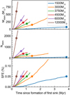 |
Fig. 1. Evolution of the total mass accreted in sink particles (top), number of sink particles (middle), and star formation efficiency (SFE, bottom) over time for all simulations. The circles indicate the value of a quantity when the simulation has SFE = 0.05. |
Projections of the density over the entire computational domain for each simulation are shown in Fig. 2. Each row is a simulation and each column shows a projection for SFE = 0%, 1.7%, 3.3%, and 5% respectively. The colour bars are centred logarithmically on the initial mean gas density of each simulation (defined as Mgas/4 pc3) and have the same range. This was chosen to visualise degrees of gas concentration between simulations. The sink particles are annotated by blue dots. From the projections, we see that most sink particles reside in regions of high column density, which, in particular at early times, is close to their region of birth.
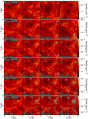 |
Fig. 2. Projections of the density over the entire computational domain from the formation of the first sink (left column) to SFE = 0.05 (right column), for each simulation. The sink particles are annotated with blue particles. The colour bars are logarithmically centred on the mean gas density of the initial gas distribution. |
3.1. Identifying multiple star systems and their formation pathways
As the sink particles accrete and interact, multiple star systems form and disintegrate. Multiple star systems were identified by:
-
Finding the sink particle pairs that are below a separation threshold and gravitationally bound (where the Epotential + Ekinetic = Etotal < 0). For our work, the maximum separation is set to 10 000 AU.
-
We then sort the pairs from lowest to highest separation.
-
A new ‘particle’ is saved with the position being the centre of mass of the bound sink particle pair and mass that is the total mass of the particle pair.
This process is carried out recursively until all bound systems with up to six components are identified. Six components are chosen as the maximum number of stars in a system because higher multiples systems tend to be short-lived with very weakly bound other companions in a highly dynamic environment, such as close to the hub-like clusters in the simulations. Sextuples are also the largest systems identified in the observations by Tobin et al. (2016b). When comparing our simulations with observations we change the approach for identifying multiple systems since three-dimensional distances and energies are not available for observations. This is discussed in Sect. 4.
When iterating, to avoid double counting sink particles that are already in a bound system, only systems are used to calculate pairs. These are either an actual sink particle if it is single, or one of the systems that was created to represent a bound pair.
As highlighted in Sect. 2.2 given the numerical resolution in our models, we can only capture core fragmentation. However, some sink particles can form isolated and unbound, but later become bound to another star. We use the birth conditions of a sink particle found in a binary or multiple to determine the pathway in which the system formed. We chronologically check bound systems, and if a new sink particle ID is found, we determine the system’s formation pathway using the following criteria:
-
Bound core fragmentation. If a sink is formed bound to another sink or system of sinks, then it was formed via bound core fragmentation.
-
Unbound core fragmentation. If a sink is formed unbound, but the sink or systems of sinks it was most bound to at birth is in the current multiple system, then it was formed via unbound core fragmentation.
-
Dynamical capture. If a sink is formed unbound, and the sink or system of sinks it was most bound to at birth is not in the current multiple system, then it was formed via dynamical capture.
These formation pathways are illustrated in Fig. 3, and examples from the simulations are shown in Fig. A.1. For systems with more than two stars, the formation pathway is determined by the newest sink particle ID ie. the most recently formed star. This classification only relies on the energy of the sink particles, and not that of the gas. Therefore, some of the systems found to be formed by unbound core fragmentation may in reality be bound, when making a detailed account of the gas distribution. We have chosen not to do this since it would entail relating different volume elements to different sink systems, which is not easily done in a unique manner and is beyond the scope of this article.
 |
Fig. 3. Illustration of the three formation pathways that a system with a new sink ID is classified into: top: if a sink is formed and is gravitationally bound to another sink or stellar system at birth (marked with a solid line), this is bound core fragmentation, middle: if a sink is formed and is gravitationally unbound at birth, but later becomes bound to the sink or stellar system it was most bound to at birth (marked with a dashed line), this is unbound core fragmentation, and bottom: if a sink is formed and is gravitationally unbound at birth, and later becomes bound to a sink or stellar system that is different to the one it was most bound to at birth, this is dynamical capture. |
In Fig. 4, we plot the separations of all multiple systems for each simulation. For binaries, this is the true separation, but for higher-order multiples, this may be the separation between stars and the centre of mass of an inner system, or two centres of mass, depending on the system configuration. If a new sink particle ID is found in a system, we also annotate its formation pathways with a marker at the initial separation of the system. In Fig. 4, the blue boxes indicate systems that formed via bound core fragmentation, the purple triangles indicate systems that formed via unbound core fragmentation, and the red circles indicate systems that formed via dynamical capture. We see that all formation pathways occur throughout the simulations. Systems that have a small initial separation likely formed via dynamical captures when a stellar fly-by of a binary resulted in a three-body interaction that expels one of the original companions and captures the fly-by star resulting in a new binary system.
 |
Fig. 4. Separation vs. SFE of all systems formed in each simulation. The markers indicate the formation pathway of the system if it contains a new sink id. Blue boxes: bound core fragmentation, purple triangles: unbound core fragmentation, red circles: dynamical capture. |
In Fig. 4, we see in each panel that many systems experience rapid orbital shrinkage, where the final separation of the systems is more than an order of magnitude smaller than the initial separation. In Fig. 5 we show the fraction of separations that are below 100 AU over time for all simulations. In all simulations, the fraction initially varies significantly due to small number statistics. However, after approximately SFE = 0.02, a gradient starts to appear with the lowest mass and highest mass simulations having 60% and 40% of separations below 100 AU, respectively. We investigate the origin of this gradient by looking at how clustered the star formation is, and orbital evolution in the following sections.
 |
Fig. 5. Fraction of all separations (between stars/stars and centre of masses/between centre of masses) that are below 100 AU, over time for all simulations. The fraction was smoothed over a window of SFE ± 5 × 10⁻⁴. The solid line shows the median of this smoothing and the shaded regions show the 1σ variation of the smoothing. |
In Fig. 6 we plot the fractions of systems that form via the different pathways for each simulation. The fractions are broadly consistent over all simulations. The fraction of systems that formed via bound core fragmentation varies between 35 − 45%, unbound core fragmentation varies between 10 − 25%, and dynamical capture varies between 35 − 50%.
 |
Fig. 6. Fractions of systems formed via the pathways (illustrated in Fig. 3) for each simulation: bound core fragmentation (blue), unbound core fragmentation (purple), and dynamical capture (red). |
The fraction of systems formed through unbound core fragmentation decreases with gas density, and hence stellar density. This is probably caused by the more dynamic environment seen in the higher-density models, leading to a lower time scale for encounters with other stars.
Overall, the fractions of that systems formed via core fragmentation (bound and unbound) are slightly higher in the lower mass simulations. This may be because the lower mass simulations require a larger over-density for protostellar cores to collapse, and this results in more systems forming via the core fragmentation pathways. This implies that star formation in lower mass GMC is more clustered than in higher mass one.
3.2. Measuring clustering with two-point correlation function
In this section we measure three-dimensional two-point correlation functions (TPCF) to gain insight into how clustered the sink particle distributions are in each simulation. A TPCF quantifies clustering by measuring all possible separations between points (for N stars, the number of separations is N(N − 1)/2)) and binning the separations into logarithmic separation bins (r). This is calculated for the observed data points (PDD(r)) and for randomly generated points that are uniformly distributed (PRR(r)). These two distributions are normalised using the number of data points and randomly generated stars to obtain:
where ND and NR is the number of data points and randomly generated points respectively. The basic TPCF (Peebles 1980) is derived by dividing the normalised distribution of the data (DD(r)) by the normalised distribution of the random points (RR(r)), that is:
If the data are clustered, the resulting TPCF will have values ≫1 in smaller separations and typically has a power law function as a function of separation with a negative slope.
To calculate a TPCF, an underlying distribution must be derived, for comparison. Given the periodic boundary conditions of our simulation, the largest separation two sinks can have is  pc which is equivalent to ∼7 × 10⁵ au. With this largest separation and the smoothing length of 16.6 AU, 10 separation bins spaced logarithmically between 10 − 106 AU were selected to calculate the TPCF. To derive the underlying distribution, 5 × 10⁵ positions were randomly generated within the simulation domain, and separations were calculated. A large number of randomly generated positions was necessary to populate the smallest separation bin. 100 instances of 5 × 10⁵ randomly generated positions were performed, and the final underlying distribution (PRR(r)) was taken to be the mean of these 100 instances, and the error is the standard deviation in a separation bin over the 100 instances.
For the simulations, the distribution (PDD(r)) is derived by calculating all separations between stars and binning the separations. The error of this distribution is taken to be the Poisson noise, because of the low number of stars per separation in the simulation, i.e.  .
.
The TPCFs for all simulations at SFE = 0.05 are shown in Fig. 7. The error bars for the TCPF are derived by summing the relative errors of DD(r) and RR(r). After calculating the TPCF a power-law is fit to the function, with a steeper slope indicating stronger clustering. Empty bins are masked to avoid poor power-law fits. At SFE = 0.05, the lower mass simulations show stronger clustering, however, this is only at one snapshot in time.
 |
Fig. 7. Two point correlation functions (TPCF) of all simulations at SFE = 0.05. The error bars on the points are the standard deviation of the TPCF values calculated against the 100 generated instances of a uniform distribution. The lines are the power law fits derived from the TPCFs up to 1 − 3 × 10⁴ AU separation bin. |
To understand how the clustering evolves over the course of the simulations, in Fig. 8 we plot fitted power-law indices for each simulation as a function of SFE. The shaded region shows the sum of the 1σ error on the power-law index plus the 1σ variation in a smoothing window. Initially, fitting a gradient is not possible due to small number statistics leading to many empty separation bins. The Mgas = 1500 M⊙ simulation has a stronger and increasing clustering throughout the simulation. Conversely, the higher-density simulations typically have shallower gradients, with little time evolution. The difference in clustering is likely due to the low-density simulation producing no stellar clusters and mostly binaries, with very few high-multiplicity systems, giving a more peaked TPCF. This is because the virial parameter is so high that stars are only formed a few at a time at density peaks with an exceptionally high over-density, leading to a very slow and stochastic star formation.
 |
Fig. 8. Gradient of two-point correlation function (TPCF) over each simulation. The smoothing was carried out in the same way as Fig. 5, however, the shaded region shows the sum of the 1σ error on the power-law index and the 1σ variation in a smoothing window. |
Observationally, the two-point correlation functions in the nearby Taurus, ρ Oph, and Orion regions are found to be a power law with exponents in the range −2 < β < −1 (Gomez et al. 1993; Larson 1995; Gomez & Lada 1998), which compares well to our results, given that exponent should be increased by one when projecting from three to two dimensions.
3.3. System formation scales
The star-forming environment may affect the initial separation of systems formed via core fragmentation pathways, which might give insight into a fragmentation scale. In Fig. 9 we plot the histogram of the initial separations of the systems formed via the three different formation pathways for each simulation pathway. For the core fragmentation pathways, the histograms are stacked in the left column, while the initial separation of dynamical capture is shown on the right column of Fig. 9.
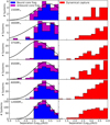 |
Fig. 9. Histograms of the initial separations of systems with new sink IDs for each simulation, for the three different formation pathways: blue: bound core fragmentation, purple: unbound core fragmentation, and red: dynamical capture. The separations were binned in log (separation), and the histogram for unbound core fragmentation is stacked on top of the bound core fragmentation histogram. The black line is the fitted Gaussian to the core fragmentation distribution. |
We fitted Gaussian distributions to the sum of the histograms for systems formed via bound and unbound core fragmentation to characterise a typical bound core fragmentation scale, dcore. The means and widths of these distributions are plotted against GMC mass in Fig. 10. The fragmentation scale appears to be smaller in denser environments, however, the typical fragmentation scale over all simulations appears to be around 103 − 3.5 AU which is consistent with observations that find a peak of around ∼3000 AU in the separation distribution of protostars (Pokhrel et al. 2018).
 |
Fig. 10. Mean fragmentation scale as a function of the GMC mass. The curve shows the peak of Gaussian distributions fitted to the (stacked) histogram of initial separations of systems formed via core fragmentation pathways plotted in Fig. 9. The error bars are the width of the Gaussian distributions and not the error on the peaks. The dashed line shows the theoretical prediction from assuming that cores on average can be described as critical Bonnor-Ebert spheres. |
If we assume that the cores on average can be described as critical mass Bonnor-Ebert spheres, the external pressure on the cores will increase with increasing cloud mass, leading to the core fragmentation scale depending inversely proportional to the square root of the cloud mass, indicated by the dashed line in Fig. 10.
The normalisation is set by assuming that the typical scale at which binaries form is similar to the radius of a critical Bonnor-Ebert core:
where ϵcore encapsulates that a binary companion will not form at the very edge of a pre-stellar core (we use ϵcore = 0.55 in the figure), and Pext is the confining pressure of the Bonnor-Ebert sphere, which can be estimated as (Haugbølle et al. 2018):
When looking at the initial separations of systems formed via dynamical capture (shown on the right column of Fig. 9), we see that for all GMC masses, the histogram increases with larger initial separations. For simulation 12 000 M⊙ the initial separation histogram plateaus beyond 1000 AU. This plateau is likely due to the higher stellar density which creates a situation where it is less probable to be captured at a large distance from a stellar system because other systems will be nearer.
3.4. Orbital evolution of the different pathways
Simulations of binary star formation via protostellar core fragmentation often show that the binaries undergo significant orbital migration. There are two classes of mechanisms that can efficiently provide migration. Dynamical friction (Chandrasekhar 1943; Ostriker 1999), slow-down due to accretion of material with lower angular momentum, and the initial high-eccentricity configuration of newly formed cores is a combination of reasons why naturally binaries with separations below ∼1000 AU suffer rapid inspiral. Prestellar cores form in general along filaments, which are kinematically cold in the direction transverse to the filament. Therefore, binaries formed through core fragmentation will initially have an angular momentum, much lower than what is required for circular motion and launch on highly eccentric orbits. This low angular momentum leads to rapid inspiral of the young binary system. Systems formed via dynamical capture must instead go through a state where they are marginally unbound and then become bound. When these systems first form, their angular momentum is therefore high, and thus, these systems are not expected to undergo fast orbital evolution. An exception is when dynamical capture is the end product of a three-body interaction, which can lead to an interchange of the stellar companions and hardening of the binary system (Reipurth 2000).
To investigate inspiral, we measure the rate of change of the semi-major axis in the 1000 and 10 000 yr after the first periastron of a system. The semi-major axis is calculated at all time steps using:
where Mtot is the total mass of the system, and ϵorb is the specific orbital energy of the system. ϵorb is calculated by summing the specific kinetic and potential energies of the system.
The median inspiral rate for systems of different formation pathways is plotted against simulation gas mass in Fig. 11. The error bars indicate the standard deviation of the measured inspiral rates. For both baselines, the inspiral rates are independent of the average density of the star-forming environment. This may be because forming systems are gravitationally decoupled from the large-scale environment and typical densities and time scales that ultimately sets the in-fall rates are set by gravity.
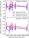 |
Fig. 11. Median inspiral rate of systems that formed via the different formation pathways (see Fig. 3) measured over the 1000 yr (top) and 10 000 yr (bottom) after the first periastron of the system vs initial gas mass of each simulation. The error bars show the standard deviation of the measured inspiral rates. |
We calculated the median inspiral rate indices over all simulations and finds that the indices are generally higher ( ) in the 1000 yr baseline compared to the 10 000 yr baseline (
 ) for all pathways. The error bars of the quoted indices are the 1σ variation over all simulations. This variation is not surprising because we expect the inspiral rate to be the greatest soon after the formation of the system, and then decrease at later stages.
For the 1000 yr baseline we do not see any significant variation between formation pathways. For the 10 000 yr baseline, we see that the median inspiral rate of systems formed via dynamical capture is marginally higher ( ) than bound core fragmentation (
 ) over all simulations.
The resulting inspiral rates measured from the 10 000 yr baseline may seem contrary to the previously stated hypothesis, but this is a result of the typical initial separation of dynamical capture systems being larger than for the core fragmentation systems (see Fig. 9). Overall, we see that many systems experience significant orbital evolution within the early stages of their lifetime.
4. Comparison with observations
We now aim to compare the multiplicity statistics produced from these simulations with observations of protostellar multiplicity. In particular, we compare our results with that of Tobin et al. (2016b) of the Perseus star-forming region using the revised statistical method described in Tobin et al. (2022). Tobin et al. (2016b) observed protostars in this region and measured how the companion frequency (CF) evolved with the separation of the components. The companion frequency as defined by Reipurth & Zinnecker (1993) is the average number of companions a star has and is given by:
where B, T, Q, ... are the number of single, binary, triple, quadruple, and higher order systems respectively.
Tobin et al. (2016b) observed a bimodal distribution in the CF versus separation, with peaks at ∼75 AU and ∼3000 AU for Class 0 and I objects. The peak at 75 AU was attributed to binaries formed via disc fragmentation while the peak at 3000 AU was attributed to systems formed via core fragmentation. However, we have shown in the previous sections that multiple systems that formed on core fragmentation scales often experience significant orbital evolution, down to separations ≤75 AU. We aim to determine what the contribution of core fragmentation is to the observed bimodal distribution.
4.1. The Perseus star-forming region and finding the best simulation for comparison
The Perseus star-forming region consists of multiple star-forming clusters. Arce et al. (2010) presents a comprehensive analysis of the mass, volume, turbulence, and star formation efficiency (SFE) of various star-forming regions in Perseus. From Arce et al. (2010) the estimated current mass, including gas mass, mass in outflows, and young stellar objects, in the L1448, NGC1333, B1-Ridge, B1, IC348, and B5 star-forming regions is approximately 3220 M⊙. The estimated total volume of all star-forming regions is 53.5 pc3, which is slightly smaller than the 43 = 64 pc3 volume of the simulations. Based on these mass and volume estimates, the Mgas = 3000 M⊙ or 3750 M⊙ simulations are best for the comparison.
To further refine which simulation is best for comparison, we calculate which simulation produces a similar number of sink particles with luminosities that would be observable by the observations of Tobin et al. (2016b).
The bimodal distribution found by Tobin et al. (2016b) is only prominent in Class 0 and I objects, and it is not seen in Class II objects. Therefore, for this comparison, we aim to target sink particles that would be classified as Class 0/I. Accretion in protostars is generally higher in the early protostellar stages than in the later stages, so an accretion limit of 10−7 M⊙ yr−1 is applied to select sinks that are likely to be in the Class 0/I stages. Observationally, Class I objects have observed accretion rates from ∼10−9 to 10−6 M⊙ yr−1, however, Class II are not observed to have accretion rates above 10−7 M⊙ yr−1 (Fiorellino et al. 2021). With the selected accretion limit we may miss some Class I objects with a low accretion rate, but avoid selecting Class II objects.
The number of Class 0/I objects observed by Tobin et al. (2016b) was 92 stars, with luminosities between 0.1 and 55 L⊙. In Tobin et al. (2022), the upper limit of the Perseus observations is stated to be approximated 120 L⊙. To find the best simulation for comparison with these observations, we calculated the number of sink particles in a simulation that would be observable. We used a lower luminosity limit of 0.1 L⊙ and upper limits of both the highest luminosity object (55 L⊙) and the theoretical maximum luminosity (120 L⊙). We assume that the luminosity is dominated by the accretion luminosity. To calculate the accretion luminosity we use:
where Ṁ is the mass accretion rate for the sink particle, R⋆ is the radius of the protostar, and facc is the fraction of potential energy from accretion that is converted into radiation. For these calculations, we take R⋆ = 2 R⊙ for all protostars and facc = 0.5 (1.e. 50% of potential energy is converted to radiation).
The evolution of the number of visible stars over time is shown in Fig. 12. We see that for all simulations, before SFE ∼0.005 essentially all sink particles are visible. However, at later times, the total number of sink particles and visible sink particles diverges. This is because older sink particles may have stopped accreting or have very low accretion rates, but newer sinks are forming which have higher accretion rates. In all simulations, a steady state in the number of visible sinks is established after SFE ∼ 0.01. Based on the steady-state visible star numbers and the number of objects observed by Tobin et al. (2016b; annotated by the horizontal dashed line in Fig. 12) the Mgas = 3750 M⊙ simulation produces the closest number of visible stars to the observations. Therefore, for further comparisons with observations, this simulation will be used.
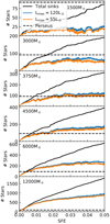 |
Fig. 12. Total number of sink particles (black) and the number of visible sink particles for the maximum luminosity of 120 L⊙ (blue), and 55 L⊙ (orange) as calculated by Eq. (7) over SFE for each simulation. The horizontal dashed line indicates the number of Class 0/I objects observed by Tobin et al. (2016b; i.e. 92 stars). |
4.2. Calculating characteristic SFE of Perseus
Observations capture the star formation evolution at a particular time, while simulations evolve over time. To make an appropriate comparison with observation, we need to find the best time for the simulations to compare with observations. To do this, we estimate a characteristic star formation efficiency of the observed star-forming regions in Perseus.
Arce et al. (2010) provides right ascension and declination boundaries for the L1448, NGC1333, B1-Ridge, B1, IC348, and B5 star-forming regions and observational estimates for the star formation efficiency in these regions. Based on the boundaries of these regions, we find how many of the Class 0 and I objects from Tobin et al. (2016b) are in each region. We find that 12 stars are in L1448, 39 stars are in NGC1333, 4 stars are in B1-Ridge, 10 stars are in B1, 13 are in IC348, 2 are in B5, and 12 are unclassified. We re-classified the unclassified stars based on which star-forming region they are closest to on the sky, and this adds 11 stars to B1-Ridge and 1 star to B1.
We then calculate a weighted average of the star-forming efficiency based on the number of stars in each region and the observed SFE. Based on Arce et al. (2010), the SFE of each region is 1.5% for L1448, 4.9% for NGC1333, 2.4% for B1-Ridge, 2.1% for B1, 9% for IC348 and 0.4% for B5. From this, the characteristic SFE we retrieve is ∼4.2%.
4.3. Data processing to make CF versus separation histogram.
To accurately carry out a comparison with observations, we must process our data the same way the observations were processed. While the true sink particle separations and separations between centres of mass for sub-systems were used to find bound systems previously, to be consistent with Tobin et al. (2022), we also calculate the separations between mid-points of components and sub-systems. Readers can refer to Fig. 1 of Tobin et al. (2022) for details on measuring separations in a multiple star system.
For some of the comparisons with observations, we save a projected midpoint-separation, for example, save the true separations projected onto the xy-plane. We also vary whether accretion and luminosity limits are applied to be consistent with Tobin et al. (2016b), and whether to count unbound pairs (pairs with projected separation < 10 000 AU). The various analysis settings are summarised in Table 2. After all the multiple systems are found based on the settings and limitations applied, we then process systems to determine how the companion frequency evolves with projected separation.
Settings used for CF vs. separation histogram.
We create 12 separation bins logarithmically spaced from 101 − 104 AU, in the same fashion of Tobin et al. (2016a) and Tobin et al. (2022). Within each bin, if a multiple system has components with separations smaller than the lower bound of the bin, it is considered a single star, and if there are components with projected separations larger than the upper bound then that system is separated into smaller systems.
It is not appropriate to compare the observations with a single time step in the simulations because accretion rates and luminosity can vary between time steps. Therefore, the CF versus separation histogram was integrated over an SFE ± 0.1% window, and the median value in each bin is used to produce the resulting histogram.
For comparison with observations, we retrieved the observations for Perseus from Tobin et al. (2022). We removed objects that were not Class 0/I and processed the data to create our histogram. We use the entire data set to produce the dashed histogram shown in Fig. 13. To approximate the correction for unbound pairs observed by Tobin et al. (2022), we recalculate the histogram only for separation with boundness likelihoods > 0.68 (refer to Table 4 of Tobin et al. 2022). This produces the solid line histogram shown in Fig. 13. The error bars are calculated using the binomial statistics described by Eq. (3) in Tobin et al. (2022).
 |
Fig. 13. Median companion frequency vs separation at star formation efficiency of 4.2%, averaged over an SFE ± 0.1% window, for the Mgas = 3750 M⊙ simulation. The solid histograms in each panel show the resulting CF vs. separation histogram for the different settings summarised in Table 2. For settings with the luminosity limits, the blue and orange show the results with an upper limit of 55 and 120 L⊙ respectively. The black dashed histogram shows the observed distribution found by Tobin et al. (2022) for all class 0/I objects, and the solid black line is the histogram derived from pairs with boundness likelihood > 0.68. The error bars are calculated using the binomial statistics described by Eq. (3) in Tobin et al. (2022). |
The results for SFE = 4.2% is shown in Fig. 13. For the 3D-Full settings, the true CF distribution of all bound systems appears to be relatively uniform at CF = 0.1. However, the CF drops significantly in the last separation bin, indicating that there are fewer true bound systems at these large separations. When observational limits are imposed in 3D-Limits, we observe an overall reduction in CF in all bins. We also see a bimodal distribution appear with peaks at ∼150 AU and ∼2000 AU. When projected onto 2D in 2D-Bound, the peak at ∼150 AU is still seen, but the larger peak is smeared out. Projecting separations into 2D will affect larger separations more than smaller separations, therefore it is expected that the CF histogram would be more affected at larger separations. When unbound pairs are counted in the 2D-Unbound analysis we see that the CF increases significantly above projected separations of > 100 AU.
4.3.1. YSO density and contamination from chance alignments
Tobin et al. (2022) correct their observations for possible chance alignments. The likelihood of a chance alignment is dependent on the observed young stellar object (YSO) density. Based on our 2D-Bound and 2D-Unbound analysis, Tobin et al. (2022) appears to have sufficiently filtered out chance alignments which may contaminate their results.
Our simulation produced significantly more unbound pairs than Tobin et al. (2016a), and we hypothesise that the chosen simulation has a significantly higher stellar density than Perseus. To investigate this we calculate the YSO density distribution for our simulation at different stages of evolution.
The YSO density is calculated using the same method described by Tobin et al. (2022). The YSO density around the sink particle is calculated using:
where r11 is the separation to the eleventh nearest visible neighbour.
We measure the YSO density at SFE = 0.5%, 1%, 2%, 3%, 4%, and 5%. The resulting cumulative distributions are plotted in Fig. 14 against the observed YSO density of Perseus for the Class 0/I objects. At SFE > 0.5%, the YSO density measured in the simulations is larger than Perseus. In the simulations, we observe that the maximum YSO density increases up to SFE = 2% and then decreases. This may reflect the initial burst of star formation in clusters, and then the later dispersal of these clusters.
 |
Fig. 14. YSO density CDF for our simulations at different SFE (blue to pink gradient). The measured YSO density for Tobin et al. (2016b, 2022) is shown by the dashed black line. |
The higher YSO density in the simulations contributes to the significantly higher CF measured with the 2D-Unbound setup in Fig. 13. The median YSO density for both Perseus and our simulation at SFE = 4% is approximately 100 pc−2, however, the simulation has an extended tail at higher densities. The highest YSO density measured among the Perseus objects is 102.8 pc−2, while the highest YSO density in the simulation at SFE = 4% is 103.8 pc−2, an order of magnitude greater. Therefore around some objects, we may expect up to 10 times more unbound pairs, contributing to the significant excess in companion frequency seen in Fig. 13.
Despite the significant increase in CF when counting unbound pairs, a peak in CF is still visible in this setup at ∼200 AU.
4.3.2. Finding best fit using two-sample KS test
While we find a bimodal distribution at the calculated characteristic SFE, we aim to determine if there is another time in the simulation where a stronger bimodal distribution is found. We carry out a two-sample Kolmogorov-Smirnov (KS) test (Massey 1951) because it is a non-parametric comparison of the shape of two distributions. While we show the result of the bimodal distribution found in Perseus, we are not concerned by the values of the resulting CF versus separation histogram, but more specifically the shape.
To calculate the KS statistic, we:
-
Order all the separations within systems observed in Perseus, and then calculate a cumulative distribution function (CDF). This distribution is normalised by dividing the CDF by the sum of all values (such that the bounds are 0 and 1).
-
For each time in the simulation, we used the 2D-Bound analysis to find the visible stars. All separations in all bound systems are sorted to produce a normalised CDF for the simulated systems.
-
Calculate the KS statistic, which is the largest vertical separation between the two normalised CDFs. We used the scipy package, which has the scipy.stats.ks_2samp function to calculate the values.
We calculate the KS statistic between SFE = 0.01 and 0.05, and we also calculate a corresponding critical value, below which, the two distributions are significantly similar. The critical value is found using:
where m and n are the number of values in each of the two samples (i.e. the number of separations, which is 39 for Perseus), and α is derived from the confidence level. We use α = 0.99, therefore if the KS statistic is below the calculated critical value, the two samples are consistent to a confidence level of 99%. We calculate KS statistics for the number of visible stars using limits in 2D-Bound analysis, for both luminosity limits.
We smoothed the KS statistic and critical value over a window of SFE = 0.01%, and the results are shown in Fig. 15. The shaded regions show the 16th and 84th percentile of the integrated values. For both luminosity limits, we see that bimodal distributions appear at various stages in the simulation. This is not surprising because we expect many systems to evolve from large to small separations, meaning that at some points in the simulation, the valley observed between ∼300 − 1000 AU is filled in.
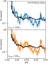 |
Fig. 15. Smoothed KS statistic measured over SFE using the 2D-Bound settings (See Table 2) for upper luminosity limits of 120 L⊙ (top) and 55 L⊙ (bottom). The smoothing window is SFE = 0.01%. The median value is plotted with an opaque line, and the shaded regions show the 16th and 84th percentile of the integrated values. The critical KS statistic (calculated with Eq. (9)) is shown by the black line. |
Based on the KS test, the time when we produce a distribution that is most consistent with the Perseus observation is at approximately SFE = 4.1% for both Lmax = 55 and 120 L⊙.
4.3.3. Best fit to observation
Based on the time of best fit found by the two-sample KS tests, we reproduce Fig. 13 for SFE = 4.1%. This is shown in Fig. 16. Although it is only slightly earlier than the CF versus separation histogram shown in Fig. 13, the bimodal distribution is more pronounced when luminosity limits are applied in 3D-Limits and 2D-Bound. While the values of the CF may vary between the simulations and observations, the positions of the peaks and the valley are in good agreement.
From this, we find that the observed bimodal distribution can be produced by multiple star formation via non-disc fragmentation pathways alone. This is not to say that disc fragmentation does not occur, but that a significant number of binaries with separations 20 − 100 AU are probably formed on core fragmentation scales and migrate. The CF values from the simulation are generally higher than observations, and in order to reduce the overall CF value, more single stars are needed.
If our simulations resolved disc fragmentation we expected a higher CF at lower separations and this may shift the inner peak to lower separations.
5. Discussion
5.1. Star formation environment on formation pathways
Our work specifically looked at whether multiple star formation on core fragmentation scales can reproduce observations of protostellar multiplicity. The minimum scale at which fragmentation occurs is set by the physics used, for example angular momentum, magnetic support, or tidal forces (Guszejnov et al. 2017; Haugbølle et al. 2018; Lee & Hennebelle 2019). Our initial condition of an isothermal equation of state (EOS), turbulent driving, and ideal MHD produces a typical fragmentation scale of approximately 1000 − 3000 AU (Figs. 9 and 10). Guszejnov et al. (2023) ran cluster simulations with a Lagrangian code with similar initial conditions (turbulent initial velocity field, ideal MHD) but also employ radiation-hydrodynamics, found similar fragmentation scales of 1000− 10 000 AU. The fragmentation scale produced by our simulations and Guszejnov et al. (2023) are consistent with observations of fragmentation in various star-forming regions having separations of a few thousand astronomical units (Palau et al. 2018; Figueira et al. 2018).
In our work, we identified the unbound core fragmentation pathway, where a star is initially born unbound, and then later becomes bound to the star or system it was most bound to at birth. Other simulations have modelled the formation of systems that were initially unbound, but through accretion, and angular momentum exchange with the surrounding medium, they become bound (Ostriker 1994; Moeckel & Bally 2007; Bate 2012; Muñoz & Lai 2015). This process has been called ‘gas-mediated capture’, and this is likely to be occurring in our unbound core fragmentation cases. Previous simulations have concluded that this mechanism would not occur frequently. In our simulations, approximately 10–25% of systems form via this mechanism (Fig. 6) with this pathway occurring more in low-density environments.
The dynamical capture pathway was thought to not occur often (Tohline 2002). However, simulations of clustered star formation and observations of young stars may suggest that flybys may occur frequently. Flybys by unbound stars have been proposed as the trigger of the excitation of spiral arms observed in some circumstellar discs Pérez et al. (2016), Cuello et al. (2019), and potentially trigger accretion bursts Borchert et al. (2022). Pfalzner & Govind (2021) used N-body simulations of the stellar dynamics in young clusters and determined that stellar flybys are probably more common than initially expected in low mass clusters, and 10%-15% of discs should show evidence of this. Pfalzner & Govind (2021) suggest that while the overall stellar density is lower in low mass star-forming regions, the distribution of stars is more clustered, which can aid stellar interactions in the central regions. In our work, we also confirm that star formation is more clustered in lower-density environments.
With the evidence that stellar flybys are not uncommon, it is not unreasonable to suggest that some flyby events may turn into dynamical capture events. Our work finds that for stars that are born unbound but later become bound, in higher-density environments, they are more likely to follow the dynamical capture pathway. Murillo et al. (2016) using SED fitting, inclination effects, and outflows, measure how coeval young multiple star systems in Perseus were. They found that approximately a third of the objects were non-coeval, suggesting these systems did not necessarily form together. This fraction is consistent with our Mgas = 3750 M⊙ simulation which also found around a third of systems follows the dynamical capture formation pathway (see Fig. 6). Our simulations also suggested that for stars that are born unbound, the fraction that follow the dynamical capture pathways increases in higher-density environments.
Once a bound binary is formed, it can proceed to evolve to smaller separations via dynamical friction with the surrounding gas. This is because in the early stages when a star is low mass in a dense environment, the dynamics are dominated by the gas. The young star dynamics are influenced by the momentum gained via accretion, and the dense wakes that form from moving through dense gas mediums (Bate & Bonnell 1997; Ostriker 1999; Stahler 2010; Kuruwita et al. 2020). Lee et al. (2019) ran simulations of clustered star formation using the MHD AMR ORION2 with similar initial conditions to our simulations and derived a model to describe the orbital decay seen in two of the formed binaries. This model describes the angular momentum evolution of the simulated binaries using:
where r* is the separation vector of the star to the centre of mass, and v∗,rel is the relative velocity between the star and the gas. The model describes the later evolution (> 100 kyr) of the simulated binaries well and finds that orbital evolution is halted when the binary is no longer embedded because there is no gas around to create drag. This formulation suggested that with a higher accretion rate, the inspiral rate is faster.
In our work, we find that the characteristic initial inspiral rates (< 10 000 yr, Fig. 11) do not vary significantly between star-forming environments (i.e. different simulations). This inspiral behaviour may eventually reflect the evolution that is modelled by Lee et al. (2019) at later times, but this is not measured in this work. Within each simulation, there is a substantial spread in the inspiral rates measured over our baselines. This may suggest that the orbital evolution is more sensitive to the local environment around the system than the overall star-forming environment. Curiously, we find that systems that formed via dynamical capture experienced faster inspiral rates when measured over the first 10 000 yr of evolution since the first periastron. This was a surprise because we hypothesised that these systems would inspiral slowly. However, many of these systems may have experienced an interaction that quickly hardens previously unbound pairs.
It is difficult to observe evidence of orbital evolution in wide binaries (a > 1000 AU) due to the long orbital periods for individual systems. However, observations of OB associations find that the velocity dispersion increases with age (Ramírez-Tannus et al. 2021). This relationship between velocity dispersion and age is suggested to be caused by the hardening of binaries, supporting orbital migration forming close binaries. However, this velocity dispersion evolution is observed over millions of years, but simulations of binary star formation from core fragmentation frequently produce binaries that experience significant orbital evolution very early on as described above.
5.2. Reproducing observations
In Sect. 4 we investigated whether our simulations reproduced the bimodal CF versus separation distributions observed in protostars in Perseus (Tobin et al. 2016b). This bimodal distribution has also been observed in Orion (Tobin et al. 2022), and Encalada et al. (2021) appear to resolve the inner peak in Ophiuchus. The valley between the two peaks has also been observed in Class I objects in various star-forming regions across the sky by Connelley et al. (2008). Because this bimodal distribution has been observed in multiple regions it is expected to be a long-lived feature.
One proposed hypothesis for the origin of a bimodal separation distribution comes from Heggie (1975) who suggested that hard binaries become harder and soft binaries become softer, leading to a bimodal separation distribution. A mechanism for orbital hardening is via the ejection of a companion. This companion can either be completely ejected from the system (becomes unbound) or pushed to a wider orbit. Many binaries in very wide orbits are found to be in triple systems, and it is hypothesised the outer companion was ejected to a wider orbit (Reipurth & Mikkola 2012). Ejections of companions and changing multiple star systems architectures also occur in gas-rich environments, like our own simulations and in other works (Bate 2012; Ryu et al. 2017).
Conversely, when the protostellar bimodal distribution was first observed in the Perseus star-forming region, the two peaks were attributed to disc fragmentation producing close binaries, and core fragmentation producing wide binaries (Tobin et al. 2016b). However, as shown throughout this paper, binaries that are formed on core fragmentation scales often experience significant orbital evolution early in their formation. We calculated CF versus separation distribution of multiple star systems, looking at the true distribution, as well as applying observational limits. We successfully produce bimodal distributions at the calculated characteristic SFE of the observed objects in Perseus (4.2%), and later find a better match to the Tobin et al. (2016b) observations at SFE = 4.1%.
The origin of the bimodal distribution in our sims appears to be driven but the inspiral of young binaries, which migrate from separations of 100–1000 s AU to tens of AU. While there are complex N-body interactions occurring in our simulations, it does not seem that the mechanism described by Heggie (1975) is dominant, at least, not on the timescales explored in this work.
As stated previously, this observed bimodal distribution may be long-lived and it is not clear if the evolutionary state of a star-forming cloud would affect when this distribution is observed. Multiple star systems form throughout all of the simulations as shown in Fig. 4, therefore we expect to constantly observe systems forming at large separations (> 1000 AU) and in-spiralling to smaller separations. The derived best fit is close to the derived characteristic SFE, and it is not clear if this is coincidental.
While the best fit between simulations and observations occurs near when the SFE of the simulation matches observations, when we look at the calculated KS statistic against the critical value in Fig. 15, we see that good statistical agreement appears throughout the evolution of the simulations. Looking at the evolution of the KS statistic, bimodal distributions with similar shapes to that observed in Perseus appear and disappear at different stages. There is an extended period where good statistical agreement is found between SFE ∼3.9–4.3%, which spans ∼52 kyr in simulation time. This bimodal distribution will be visible for approximately 10% of the simulation run time. This makes it clear that the feature in our simulation is not spurious, but is a robust feature.
Overall, we can reproduce the observed bimodal distribution in protostellar CF using multiple star systems formed on core fragmentation scales only due to orbital migration. This is not to say that disc fragmentation does not occur, but that a significant fraction of closer binaries (20 − 100 AU) can form via non-disc fragmentation pathways.
6. Limitations and caveats
6.1. Numerical resolution
On the highest level of refinement, the resolution of our simulations is 50 AU, which means typical circumstellar disc sizes (∼75 AU; Cox et al. 2017; Ansdell et al. 2018) are only resolved over a couple of cells. However, this work only investigates star formation from molecular cloud fragmentation, therefore, resolving discs is not crucial to this work.
Discs are an important part of the mechanism that determines how much mass is accreted onto stars, and what is ejected via outflows, and this is discussed in the next section.
The sink particle motion is calculated using a leap-frog integrator, and the smoothing length is a third of a cell length on the highest resolution, i.e. 16.6 AU. The sink particle motion is calculated using the gravitational potential from both other sink particles and the gas potential. The integrator can accurately calculate the N-body particles until the separation is near the softening length. However, the gravitational potential contribution from the gas can be less resolved as the two sink particles approach separations near the softening length.
Overall, the numerical resolution is limited near and sink particles, and may not accurately simulate orbital evolution when the separations are comparable to the softening length. The work in this paper has primarily focused on resolving the bimodal distribution observed in protostars, with the inner peak at projected separations of 75 AU. With our simulation setup, we can sufficiently resolve this inner peak.
6.2. Non-ideal MHD effects and resolving outflows
Our simulations compute the ideal-magnetohydrodynamic equations. For molecular clouds, the typical fractional ionisation (abundance of electrons) is ∼10−6 − 10−8. With this ionisation fraction, ambipolar diffusion is present to help dissipate magnetic field flux to allow protostellar cores to collapse. While we do not explicitly include ambipolar diffusion in the computation of the MHD, Hennebelle & Inutsuka (2019) argue that the numerical diffusion naturally present in hydrodynamic simulation is sufficient to reproduce the effect of ambipolar diffusion. Other non-ideal effects are not dominant in the molecular cloud regime, however, Wurster et al. (2019) investigated full non-ideal MHD with clustered star formation with smoothed particle hydrodynamic simulations and found there is less magnetic breaking leading to discs forming more easily. With our resolution, we do not resolve discs, therefore, we do not expect the inclusion of other non-ideal effects to affect our results.
Magnetic fields are responsible for launching jets and outflows which return mass and momentum to the surrounding protostellar environment. With the resolution of 50 AU, jets are not self-consistently produced while weak outflows can be produced with larger discs. Not resolving outflows will not affect the motion of the sink particles significantly, but outflows regulate what fraction of mass is accreted onto the star and what is lost via outflows. As described in Sect. 2.2, we assume a mass accretion fraction of 50%. The fraction of mass that is accreted is not well constrained and various disc wind models give accretion fractions from 40-90% (Seifried et al. 2012; Fendt & Sheikhnezami 2013). Observations of T-Tauri stars find mass accretion fractions of 50–99% (Nisini et al. 2018), and observations of Herbig-Haro objects find fractions of ∼90% (Ellerbroek et al. 2013).
The accretion fraction used in our simulations may be on the lower end of typical accretion fractions but it is still consistent with models and observations.
6.3. Radiation feedback
An isothermal equation of state is used in our simulations, therefore, the internal energy remains constant throughout the simulations. This equation of state is satisfactory for our simulations because with our resolution we do not enter the regime where adiabatic heating of protostellar cores occurs (∼3.8 × 10⁻¹³ g cm−3; Masunaga & Inutsuka 2000). This is because the density threshold for sink particle formation does not exceed 1.3 × 10⁻¹⁴ g cm−3.
While an isothermal equation of state is justified in this work for the resolution at which we simulate hydrodynamics, the sink particles are used as proxies for stars, which would be able to produce radiation feedback. Radiation pressure from star formation can inject energy back into the star-forming environment, however, radiative MHD simulations carried out by Rosen & Krumholz (2020) find that magnetic fields are dominant over radiation pressure feedback, even in massive stars. Observations also suggest that gas temperature may not have a strong impact on fragmentation and rather, mass and density are key factors in fragmentation Murillo et al. (2018).
Radiation feedback from the protostars is also found to suppress disc fragmentation (Offner 2011). However, in this work, we are only concerned with multiple star formation on core fragmentation scales.
7. Summary and conclusions
We present a numerical study investigating protostellar multiplicity in star-forming environments of varying density. We find the following main results.
Multiple star formation pathways. Three main formation pathways were identified in this study, which were bound core fragmentation, unbound core fragmentation, and dynamical capture. Approximately a third of systems with a new star form via dynamical capture, independent of the star-forming environment. This is consistent with observations that find approximately a third of protostellar binaries appear to not be coeval (Murillo et al. 2016).
Orbital evolution. We find that systems that form on core fragmentation scales undergo significant orbital evolution. The median inspiral rate when measured on 1 000 and 10 000 year baselines does not vary with star-forming environments. However, within a single simulation, the spread in inspiral rates is large, implying that the orbital evolution is probably most strongly affected by the local environment around the system, rather than the larger star-forming environment.
We find the inspiral rate when measured over 10 000 years does begin to segregate based on formation pathways, with systems that form via dynamical capture in-spiralling faster than those formed via bound core fragmentation. This suggests that systems that form via dynamical capture undergo an interaction that hardens the system quickly, and prolongs the inspiral process, while bound core fragmentation systems reach a steady orbit sooner.
Reproducing observed protostellar bimodal separation distribution. We used the simulation with the global properties closest to the Perseus star-forming region, and derived companion frequency versus separation distributions. When selecting SFEs in the model that matches the observed SFE of Perseus, we find a similar bimodal distribution to the one observed in Perseus (Tobin et al. 2016b, 2022) when using the same selection criteria for the sink particles as in the observations. This is due to orbital migration from large separations to 20 − 100 AU. The valley between the peaks is less defined than in the observations and is not globally present throughout the evolution, but only in a range of SFEs from 3.9% to 4.3%.
Overall our results are compatible with core fragmentation and dynamical capture being the only sources of multiplicity for separations above 20 AU, without the need for any contribution from disc fragmentation. Multiple star formation on core fragmentation scales (100 s to 1000 s of AU) can follow different pathways, but many systems experience significant orbital evolution resulting in closer separations. The star formation environment may influence which pathways are more prominent, but the subsequent inspiral rate is independent of the global environment. The result of the orbital evolution is that multiple star systems with a range of separations are produced, including close binaries. This orbital evolution naturally leads to the observed bimodal distribution seen in the Perseus star-forming region when considering large enough SFEs.
Acknowledgments
We thank the anonymous referee for their insightful comments and suggestions. The research leading to these results has received funding from the Independent Research Fund Denmark through grant No. DFF 8021-00350B (TH, RLK). This project has received funding from the European Union’s Horizon 2020 research and innovation Program under the Marie Sklodowska-Curie grant agreement No. 847523 ‘INTERACTIONS’. The astrophysics HPC facility at the University of Copenhagen, supported by research grants from the Carlsberg, Novo, and Villum foundations, was used for carrying out the simulations and analysis, as well as long-term storage of the results. RLK also acknowledges funding from the Klaus Tschira Foundation. yt (Turk et al. 2011) was used to help visualise and analyse these simulations.
References
- Ansdell, M., Williams, J. P., Trapman, L., et al. 2018, ApJ, 859, 21 [NASA ADS] [CrossRef] [Google Scholar]
- Arce, H. G., Borkin, M. A., Goodman, A. A., Pineda, J. E., & Halle, M. W. 2010, ApJ, 715, 1170 [NASA ADS] [CrossRef] [Google Scholar]
- Armitage, P. J., & Clarke, C. J. 1997, MNRAS, 285, 540 [NASA ADS] [CrossRef] [Google Scholar]
- Bate, M. R. 2012, MNRAS, 419, 3115 [NASA ADS] [CrossRef] [Google Scholar]
- Bate, M. R. 2019, MNRAS, 484, 2341 [NASA ADS] [CrossRef] [Google Scholar]
- Bate, M. R., & Bonnell, I. A. 1997, MNRAS, 285, 33 [NASA ADS] [CrossRef] [Google Scholar]
- Bate, M. R., Bonnell, I. A., & Price, N. M. 1995, MNRAS, 277, 362 [Google Scholar]
- Borchert, E. M. A., Price, D. J., Pinte, C., & Cuello, N. 2022, MNRASL, 510, L37 [Google Scholar]
- Chandrasekhar, S. 1943, ApJ, 97, 255 [Google Scholar]
- Chen, X., Arce, H. G., Zhang, Q., et al. 2013, ApJ, 768, 110 [Google Scholar]
- Connelley, M. S., Reipurth, B., & Tokunaga, A. T. 2008, AJ, 135, 2526 [NASA ADS] [CrossRef] [Google Scholar]
- Cox, E. G., Harris, R. J., Looney, L. W., et al. 2017, ApJ, 851, 83 [Google Scholar]
- Cuello, N., Montesinos, M., Stammler, S. M., Louvet, F., & Cuadra, J. 2019, A&A, 622, A43 [NASA ADS] [CrossRef] [EDP Sciences] [Google Scholar]
- Ellerbroek, L. E., Podio, L., Kaper, L., et al. 2013, A&A, 551, A5 [NASA ADS] [CrossRef] [EDP Sciences] [Google Scholar]
- Elliott, P., & Bayo, A. 2016, MNRAS, 459, 4499 [NASA ADS] [CrossRef] [Google Scholar]
- Encalada, F. J., Looney, L. W., Tobin, J. J., et al. 2021, ApJ, 913, 149 [NASA ADS] [CrossRef] [Google Scholar]
- Federrath, C., & Klessen, R. S. 2012, ApJ, 761, 156 [Google Scholar]
- Federrath, C., Banerjee, R., Clark, P. C., & Klessen, R. S. 2010, ApJ, 713, 269 [NASA ADS] [CrossRef] [Google Scholar]
- Federrath, C., Schrön, M., Banerjee, R., & Klessen, R. S. 2014, ApJ, 790, 128 [NASA ADS] [CrossRef] [Google Scholar]
- Fendt, C., & Sheikhnezami, S. 2013, ApJ, 774, 12 [Google Scholar]
- Figueira, M., Bronfman, L., Zavagno, A., et al. 2018, A&A, 616, L10 [NASA ADS] [CrossRef] [EDP Sciences] [Google Scholar]
- Fiorellino, E., Manara, C. F., Nisini, B., et al. 2021, A&A, 650, A43 [NASA ADS] [CrossRef] [EDP Sciences] [Google Scholar]
- Gammie, C. F. 2001, ApJ, 553, 174 [Google Scholar]
- Gomez, M., & Lada, C. J. 1998, AJ, 115, 1524 [CrossRef] [Google Scholar]
- Gomez, M., Hartmann, L., Kenyon, S. J., & Hewett, R. 1993, AJ, 105, 1927 [NASA ADS] [CrossRef] [Google Scholar]
- Gong, H., & Ostriker, E. C. 2013, ApJSS, 204, 8 [NASA ADS] [CrossRef] [Google Scholar]
- Guszejnov, D., Hopkins, P. F., & Krumholz, M. R. 2017, MNRAS, 468, 4093 [CrossRef] [Google Scholar]
- Guszejnov, D., Raju, A. N., Offner, S. S. R., et al. 2023, MNRAS, 518, 4693 [Google Scholar]
- Haugbølle, T., Padoan, P., & Nordlund, Å. 2018, ApJ, 854, 35 [CrossRef] [Google Scholar]
- Heggie, D. C. 1975, MNRAS, 173, 729 [NASA ADS] [CrossRef] [Google Scholar]
- Hennebelle, P., & Inutsuka, S.-I. 2019, Front. Astron. Space Sci., 6 [Google Scholar]
- Krumholz, M. R., McKee, C. F., & Klein, R. I. 2004, ApJ, 611, 399 [NASA ADS] [CrossRef] [Google Scholar]
- Kuruwita, R. L., Federrath, C., & Ireland, M. 2017, MNRAS, 470, 1626 [NASA ADS] [CrossRef] [Google Scholar]
- Kuruwita, R. L., Federrath, C., & Haugbølle, T. 2020, A&A, 641, A59 [NASA ADS] [CrossRef] [EDP Sciences] [Google Scholar]
- Larson, R. B. 1995, MNRAS, 272, 213 [NASA ADS] [Google Scholar]
- Lee, J.-E., Lee, S., Dunham, M. M., et al. 2017, Nat. Astron., 1, 0172 [NASA ADS] [CrossRef] [Google Scholar]
- Lee, A. T., Offner, S. S. R., Kratter, K. M., Smullen, R. A., & Li, P. S. 2019, ApJ, 887, 232 [NASA ADS] [CrossRef] [Google Scholar]
- Lee, Y.-N., & Hennebelle, P. 2019, A&A, 622, A125 [NASA ADS] [CrossRef] [EDP Sciences] [Google Scholar]
- Massey, F. J. 1951, J. Am. Stat. Assoc., 46, 68 [CrossRef] [Google Scholar]
- Masunaga, H., & Inutsuka, S.-I. 2000, ApJ, 531, 350 [NASA ADS] [CrossRef] [Google Scholar]
- Moe, M., & Di Stefano, R. 2017, ApJS, 230, 15 [Google Scholar]
- Moeckel, N., & Bally, J. 2007, ApJ, 656, 275 [NASA ADS] [CrossRef] [Google Scholar]
- Muñoz, D. J., & Lai, D. 2015, PNAS, 112, 9264 [CrossRef] [Google Scholar]
- Murillo, N. M., van Dishoeck, E. F., Tobin, J. J., & Fedele, D. 2016, A&A, 592, A56 [NASA ADS] [CrossRef] [EDP Sciences] [Google Scholar]
- Murillo, N. M., van Dishoeck, E. F., Tobin, J. J., Mottram, J. C., & Karska, A. 2018, A&A, 620, A30 [NASA ADS] [CrossRef] [EDP Sciences] [Google Scholar]
- Nisini, B., Antoniucci, S., Alcalá, J. M., et al. 2018, A&A, 609, A87 [EDP Sciences] [Google Scholar]
- Offner, S. S. R. 2011, Proc. Int. Astron. Union, 6, 231 [Google Scholar]
- Offner, S. S. R., Moe, M., Kratter, K. M., et al. 2022, ArXiv e-prints [arXiv:2203.10066] [Google Scholar]
- Ostriker, E. C. 1994, ApJ, 424, 292 [NASA ADS] [CrossRef] [Google Scholar]
- Ostriker, E. C. 1999, ApJ, 513, 252 [Google Scholar]
- Padoan, P., & Nordlund, Å. 2011, ApJ, 730, 40 [Google Scholar]
- Padoan, P., Haugbølle, T., & Nordlund, Å. 2012, ApJ, 759, L27 [Google Scholar]
- Palau, A., Zapata, L. A., Román-Zúñiga, C. G., et al. 2018, ApJ, 855, 24 [Google Scholar]
- Parker, R. J., & Meyer, M. R. 2014, MNRAS, 442, 3722 [NASA ADS] [CrossRef] [Google Scholar]
- Peebles, P. J. E. 1980, The Large-scale Structure of the Universe (Princeton University Press) [Google Scholar]
- Pérez, L. M., Carpenter, J. M., Andrews, S. M., et al. 2016, Science, 353, 1519 [Google Scholar]
- Pfalzner, S., & Govind, A. 2021, ApJ, 921, 90 [NASA ADS] [CrossRef] [Google Scholar]
- Pokhrel, R., Myers, P. C., Dunham, M. M., et al. 2018, ApJ, 853, 5 [NASA ADS] [CrossRef] [Google Scholar]
- Ramírez-Tannus, M. C., Backs, F., de Koter, A., et al. 2021, A&A, 645, L10 [NASA ADS] [CrossRef] [EDP Sciences] [Google Scholar]
- Reipurth, B. 2000, AJ, 120, 3177 [CrossRef] [Google Scholar]
- Reipurth, B., & Mikkola, S. 2012, Nature, 492, 221 [NASA ADS] [CrossRef] [Google Scholar]
- Reipurth, B., & Zinnecker, H. 1993, A&A, 278, 81 [NASA ADS] [Google Scholar]
- Rosen, A. L., & Krumholz, M. R. 2020, AJ, 160, 78 [NASA ADS] [CrossRef] [Google Scholar]
- Ryu, T., Leigh, N. W. C., & Perna, R. 2017, MNRAS, 470, 2 [CrossRef] [Google Scholar]
- Saiki, Y., & Machida, M. N. 2020, ApJ, 897, L22 [NASA ADS] [CrossRef] [Google Scholar]
- Seifried, D., Pudritz, R. E., Banerjee, R., Duffin, D., & Klessen, R. S. 2012, MNRAS, 422, 347 [NASA ADS] [CrossRef] [Google Scholar]
- Stahler, S. W. 2010, MNRAS, 402, 1758 [NASA ADS] [CrossRef] [Google Scholar]
- Takaishi, D., Tsukamoto, Y., & Suto, Y. 2021, PASJ, 73, L25 [NASA ADS] [CrossRef] [Google Scholar]
- Teyssier, R. 2002, A&A, 385, 337 [CrossRef] [EDP Sciences] [Google Scholar]
- Tobin, J. J., Kratter, K. M., Persson, M. V., et al. 2016a, Nature, 538, 483 [NASA ADS] [CrossRef] [Google Scholar]
- Tobin, J. J., Looney, L. W., Li, Z.-Y., et al. 2016b, ApJ, 818, 73 [CrossRef] [Google Scholar]
- Tobin, J. J., Offner, S. S. R., Kratter, K. M., et al. 2022, ApJ, 925, 39 [NASA ADS] [CrossRef] [Google Scholar]
- Tohline, J. E. 2002, ARA&A, 40, 349 [NASA ADS] [CrossRef] [Google Scholar]
- Tomisaka, K. 2000, ApJ, 528, L41 [NASA ADS] [CrossRef] [Google Scholar]
- Tomisaka, K. 2002, ApJ, 575, 306 [NASA ADS] [CrossRef] [Google Scholar]
- Turk, M. J., Smith, B. D., Oishi, J. S., et al. 2011, ApJS, 192, 9 [NASA ADS] [CrossRef] [Google Scholar]
- Wurster, J., Bate, M. R., & Price, D. J. 2018, MNRAS, 475, 1859 [NASA ADS] [CrossRef] [Google Scholar]
- Wurster, J., Bate, M. R., & Price, D. J. 2019, MNRAS, 489, 1719 [NASA ADS] [CrossRef] [Google Scholar]
Appendix A: Examples of formation pathways taken from simulation
In Figure A.1, we show examples of the formation pathways described in Figure 3 in Section 3.1. A system’s formation pathway was determined by the sink particle data, which is written out at a ∼2 yr cadence. Due to the coarse cadence of the hydrodynamic data (∼22 kyr), not all systems could be plotted.
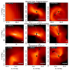 |
Fig. A.1. Shows examples of the formation pathways described in Figure 3 in Section 3.1. Projections were taken from candidates in the Mgas = 3000 M⊙ simulation. The grey bar in the bottom right of each panel annotates 1000 AU. The time annotated in the top left of each panel indicates the time with respect to the star that is centred on for each pathway. |
The projections are centred on the primary component in the bound core fragmentation pathway, and on the secondary companion in the other formation pathways. The position of the pre-sink formation frame (the projections in the left column) is estimated using the initial velocity of the centred star at birth. The projections are integrated over a box, where the side length is 2 × (rsep_max + 500 AU) in the xy-plane, where rsep_max is the maximum separation between the centred sink particle and other sink particles related to the star.
The colour bar of each projection spans three orders of magnitude and is centred on the mean density in the projection. At the bottom of each panel, 1000 AU is annotated by a grey bar. A solid line between stars indicates a bound relationship (i.e. Epot > Ekin). A dashed line signifies a relationship where the system is unbound, but this is the system that the centred sink has the lowest energy relationship with.
The centred star and the sink particle or system that the centred star is most bound to at birth are annotated by yellow stars. Other stars are annotated in red.
All Tables
All Figures
 |
Fig. 1. Evolution of the total mass accreted in sink particles (top), number of sink particles (middle), and star formation efficiency (SFE, bottom) over time for all simulations. The circles indicate the value of a quantity when the simulation has SFE = 0.05. |
| In the text | |
 |
Fig. 2. Projections of the density over the entire computational domain from the formation of the first sink (left column) to SFE = 0.05 (right column), for each simulation. The sink particles are annotated with blue particles. The colour bars are logarithmically centred on the mean gas density of the initial gas distribution. |
| In the text | |
 |
Fig. 3. Illustration of the three formation pathways that a system with a new sink ID is classified into: top: if a sink is formed and is gravitationally bound to another sink or stellar system at birth (marked with a solid line), this is bound core fragmentation, middle: if a sink is formed and is gravitationally unbound at birth, but later becomes bound to the sink or stellar system it was most bound to at birth (marked with a dashed line), this is unbound core fragmentation, and bottom: if a sink is formed and is gravitationally unbound at birth, and later becomes bound to a sink or stellar system that is different to the one it was most bound to at birth, this is dynamical capture. |
| In the text | |
 |
Fig. 4. Separation vs. SFE of all systems formed in each simulation. The markers indicate the formation pathway of the system if it contains a new sink id. Blue boxes: bound core fragmentation, purple triangles: unbound core fragmentation, red circles: dynamical capture. |
| In the text | |
 |
Fig. 5. Fraction of all separations (between stars/stars and centre of masses/between centre of masses) that are below 100 AU, over time for all simulations. The fraction was smoothed over a window of SFE ± 5 × 10⁻⁴. The solid line shows the median of this smoothing and the shaded regions show the 1σ variation of the smoothing. |
| In the text | |
 |
Fig. 6. Fractions of systems formed via the pathways (illustrated in Fig. 3) for each simulation: bound core fragmentation (blue), unbound core fragmentation (purple), and dynamical capture (red). |
| In the text | |
 |
Fig. 7. Two point correlation functions (TPCF) of all simulations at SFE = 0.05. The error bars on the points are the standard deviation of the TPCF values calculated against the 100 generated instances of a uniform distribution. The lines are the power law fits derived from the TPCFs up to 1 − 3 × 10⁴ AU separation bin. |
| In the text | |
 |
Fig. 8. Gradient of two-point correlation function (TPCF) over each simulation. The smoothing was carried out in the same way as Fig. 5, however, the shaded region shows the sum of the 1σ error on the power-law index and the 1σ variation in a smoothing window. |
| In the text | |
 |
Fig. 9. Histograms of the initial separations of systems with new sink IDs for each simulation, for the three different formation pathways: blue: bound core fragmentation, purple: unbound core fragmentation, and red: dynamical capture. The separations were binned in log (separation), and the histogram for unbound core fragmentation is stacked on top of the bound core fragmentation histogram. The black line is the fitted Gaussian to the core fragmentation distribution. |
| In the text | |
 |
Fig. 10. Mean fragmentation scale as a function of the GMC mass. The curve shows the peak of Gaussian distributions fitted to the (stacked) histogram of initial separations of systems formed via core fragmentation pathways plotted in Fig. 9. The error bars are the width of the Gaussian distributions and not the error on the peaks. The dashed line shows the theoretical prediction from assuming that cores on average can be described as critical Bonnor-Ebert spheres. |
| In the text | |
 |
Fig. 11. Median inspiral rate of systems that formed via the different formation pathways (see Fig. 3) measured over the 1000 yr (top) and 10 000 yr (bottom) after the first periastron of the system vs initial gas mass of each simulation. The error bars show the standard deviation of the measured inspiral rates. |
| In the text | |
 |
Fig. 12. Total number of sink particles (black) and the number of visible sink particles for the maximum luminosity of 120 L⊙ (blue), and 55 L⊙ (orange) as calculated by Eq. (7) over SFE for each simulation. The horizontal dashed line indicates the number of Class 0/I objects observed by Tobin et al. (2016b; i.e. 92 stars). |
| In the text | |
 |
Fig. 13. Median companion frequency vs separation at star formation efficiency of 4.2%, averaged over an SFE ± 0.1% window, for the Mgas = 3750 M⊙ simulation. The solid histograms in each panel show the resulting CF vs. separation histogram for the different settings summarised in Table 2. For settings with the luminosity limits, the blue and orange show the results with an upper limit of 55 and 120 L⊙ respectively. The black dashed histogram shows the observed distribution found by Tobin et al. (2022) for all class 0/I objects, and the solid black line is the histogram derived from pairs with boundness likelihood > 0.68. The error bars are calculated using the binomial statistics described by Eq. (3) in Tobin et al. (2022). |
| In the text | |
 |
Fig. 14. YSO density CDF for our simulations at different SFE (blue to pink gradient). The measured YSO density for Tobin et al. (2016b, 2022) is shown by the dashed black line. |
| In the text | |
 |
Fig. 15. Smoothed KS statistic measured over SFE using the 2D-Bound settings (See Table 2) for upper luminosity limits of 120 L⊙ (top) and 55 L⊙ (bottom). The smoothing window is SFE = 0.01%. The median value is plotted with an opaque line, and the shaded regions show the 16th and 84th percentile of the integrated values. The critical KS statistic (calculated with Eq. (9)) is shown by the black line. |
| In the text | |
 |
Fig. 16. Same as Fig. 13, but for SFE = 4.1%. |
| In the text | |
 |
Fig. A.1. Shows examples of the formation pathways described in Figure 3 in Section 3.1. Projections were taken from candidates in the Mgas = 3000 M⊙ simulation. The grey bar in the bottom right of each panel annotates 1000 AU. The time annotated in the top left of each panel indicates the time with respect to the star that is centred on for each pathway. |
| In the text | |
Current usage metrics show cumulative count of Article Views (full-text article views including HTML views, PDF and ePub downloads, according to the available data) and Abstracts Views on Vision4Press platform.
Data correspond to usage on the plateform after 2015. The current usage metrics is available 48-96 hours after online publication and is updated daily on week days.
Initial download of the metrics may take a while.


