| Issue |
A&A
Volume 673, May 2023
|
|
|---|---|---|
| Article Number | A134 | |
| Number of page(s) | 17 | |
| Section | Stellar structure and evolution | |
| DOI | https://doi.org/10.1051/0004-6361/202345845 | |
| Published online | 18 May 2023 | |
The role of magnetic fields in the formation of multiple massive stars
1
Université Paris Cité, CNRS, AstroParticule et Cosmologie, 10 Rue Alice Domon et Léonie Duquet, 75013 Paris, France
e-mail: This email address is being protected from spambots. You need JavaScript enabled to view it.
2
Université Paris Cité, Université Paris-Saclay, CEA, CNRS, AIM, Orme des Merisiers, 91190 Gif-sur-Yvette, France
3
École Normale Supérieure de Lyon, CRAL, UMR CNRS 5574, Université Lyon I, 46 Allée d’Italie, 69364 Lyon Cedex 07, France
Received:
4
January
2023
Accepted:
7
March
2023
Abstract
Context. Most massive stars are located in multiple stellar systems. Magnetic fields are believed to be essential in the accretion and ejection processes around single massive protostars.
Aims. Our aim is to unveil the influence of magnetic fields in the formation of multiple massive stars, in particular on the fragmentation modes and properties of the multiple protostellar system.
Methods. Using RAMSES, we follow the collapse of a massive pre-stellar core with (non-ideal) radiation-(magneto-)hydrodynamics. We choose a setup that promotes multiple stellar system formation in order to investigate the influence of magnetic fields on the multiple system’s properties.
Results. In the purely hydrodynamical models, we always obtain (at least) binary systems following the fragmentation of an axisymmetric density bump in a Toomre-unstable disk around the primary sink. This result sets the frame for further study of stellar multiplicity. When more than two stars are present in these early phases, their gravitational interaction triggers mergers until there are only two stars left. The following gas accretion increases their orbital separation, and hierarchical fragmentation occurs so that both stars host a comparable disk as well as a stellar system that then also forms a similar disk. Disk-related fragmenting structures are qualitatively resolved when the finest resolution is approximately 1/20 of the disk radius. We identify several modes of fragmentation: Toomre-unstable disk fragmentation, arm-arm collision, and arm-filament collision. Disks grow in size until they fragment and become truncated as the newly formed companion gains mass. When including magnetic fields, the picture evolves: The primary disk is initially elongated into a bar; it produces less fragments; disk formation and arm-arm collision are captured at comparatively higher resolution; and arm-filament collision is absent. Magnetic fields reduce the initial orbital separation but do not affect its further evolution, which is mainly driven by gas accretion. With magnetic fields, the growth of individual disks is regulated even in the absence of fragmentation or truncation.
Conclusions. Hierarchical fragmentation is seen in unmagnetized and magnetized models. Magnetic fields, including non-ideal effects, are important because they remove certain fragmentation modes and limit the growth of disks, which is otherwise only limited through fragmentation.
Key words: stars: formation / stars: massive / accretion / accretion disks / magnetohydrodynamics (MHD) / methods: numerical / binaries: general
© The Authors 2023
 Open Access article, published by EDP Sciences, under the terms of the Creative Commons Attribution License (https://creativecommons.org/licenses/by/4.0), which permits unrestricted use, distribution, and reproduction in any medium, provided the original work is properly cited.
This article is published in open access under the Subscribe to Open model. This email address is being protected from spambots. You need JavaScript enabled to view it. to support open access publication.
1. Introduction
Massive stars are very often located in multiple systems (Sana et al. 2012; Chini et al. 2012; Duchêne & Kraus 2013), and interest in the importance of magnetic fields for massive star formation has been growing recently (Girart et al. 2009; for a review, we refer the reader to Tsukamoto et al. 2022), but the exact role of magnetic fields in the formation of multiple massive stars is not yet clear. In addition to the role of magnetic fields in the origin of massive protostellar outflows, as predicted by Kölligan & Kuiper (2018), Commerçon et al. (2022), Mignon-Risse et al. (2021a), Oliva & Kuiper (2023a) and detected with unprecedented resolution by Moscadelli et al. (2022) using masers, magnetic fields are expected to limit gas fragmentation and therefore are certainly important in multiple massive star formation (Añez-López et al. 2020). Numerical studies had to tackle both core and disk fragmentation since their relative contribution to the formation of multiple systems remains to be evaluated, both in the low-mass and high-mass stellar regimes. Indeed, disk fragmentation has been shown theoretically (Adams et al. 1989; Shu et al. 1990; Bonnell & Bate 1994), and it has more recently been observed thanks to high angular resolution facilities such as the Atacama Larga Millimeter/submillimeter Array (ALMA; e.g., Ilee et al. 2018; Johnston et al. 2020a,b). So far, in the case of high-mass star formation, the interplay between radiation on small scales and magnetic fields has been shown to limit core fragmentation (Commerçon et al. 2011a; Myers et al. 2013) in the ideal magneto-hydrodynamical (MHD) regime (i.e., with a perfect coupling between magnetic fields and the dust-gas-mixture). In the case of low-mass pre-stellar cores, this was shown in Commerçon et al. (2010) with radiative transfer being accounted for, which followed the study by Hennebelle & Teyssier (2008) without radiative transfer. At the scale of turbulent molecular clouds, core fragmentation inhibition by magnetic pressure has been shown in a number of studies, such as Federrath & Klessen (2012; see also the review by Padoan et al. 2014 and more recently the study of Lebreuilly et al. 2021). Incorporating ambipolar diffusion, a non-ideal MHD effect describing ion-neutral drift, the ability of magnetic fields to reduce disk fragmentation has been further shown in the study of Mignon-Risse et al. (2021b), which is oriented toward massive star formation.
Observationally, the presence and influence of magnetic fields either in massive star formation or in multiple protostellar systems has been increasingly constrained thanks to polarization measurements. The relative orientation of the field lines with respect to structures of interest (see e.g., Cox et al. 2022) has shown how the gas dynamics are coupled to the magnetic field topology. Furthermore, in a hub-filament structure (a structure which could be crucial in general for massive star formation; see the review by Motte et al. 2018), the strength of magnetic fields has been found to be comparable to gravity (Wang et al. 2019; Añez-López et al. 2020). In the low-mass star formation context, the possible interplay between rotation and magnetic fields in gas fragmentation has been exposed by Galametz et al. (2020) with the submillimeter array (SMA). In addition, the magnetic field topology in a circumbinary disk around low-mass protostellar objects has also been revealed by Alves et al. (2018) using ALMA polarization observations, showing it to be active at launching outflows (Alves et al. 2017). These results suggest a long-lasting influence over the entire protostellar phase.
The present paper builds on recent numerical results. Disk fragmentation in a centrally condensed system has been recently studied by Oliva & Kuiper (2020) and Mignon-Risse et al. (2023, hereafter Paper I). Those works focused on the properties of gaseous fragments forming in an accretion disk around a massive protostar modeled as a sink cell (in Oliva & Kuiper 2020) or sink particle (in Mignon-Risse et al. 2023), for which spiral arms play a prominent role. However, those studies explored one case in which a disk forms around a central massive protostar and neglected magnetic fields. Hence, we propose to give a complementary point of view by focusing on the formation of multiple stellar systems (described by sink particles) and studying the consequences of introducing magnetic fields.
Our choice of physical ingredients is well suited for studying protostellar disk fragmentation. First of all, non-ideal MHD is found to impact the disk formation by circumventing the so-called magnetic braking catastrophe (see Wurster & Li 2018 and references therein) and affecting subsequent disk properties that can impact disk fragmentation. In fact, the fragmentation critical length (the so-called Jeans length, Jeans 1902) depends on local pressures, mainly thermal pressure and magnetic pressure. Ambipolar diffusion (i.e., the drift between the ions and the neutrals) has been shown to produce vertically thermally supported disks rather than magnetically supported disks, as in the ideal MHD case (see e.g., Masson et al. 2016 in the low-mass and Commerçon et al. 2022 in the high-mass regime), of smaller size than in the hydrodynamical case. We note that another non-ideal MHD effect, Ohmic dissipation, produces a thermally supported midplane where fragmentation should occur in the massive protostellar context (Oliva & Kuiper 2023b). Moreover, when including all three non-ideal MHD effects (ambipolar diffusion, Ohmic dissipation, Hall effect) in low-mass pre-stellar core collapse calculations, Wurster & Bate (2019) found less disk fragmentation in their magnetized models than in their purely hydrodynamical models. For these reasons, we include MHD with ambipolar diffusion in our magnetized models, as those are already implemented in the RAMSES code (Teyssier 2002; Masson et al. 2012). Finally, radiative transfer and its coupling to hydrodynamics are taken into account in order to accurately compute the gas temperature, essential for accurate Jeans instability modeling. In that view, we use RAMSES with state-of-the-art physical ingredients: radiative transfer and MHD with ambipolar diffusion.
The combination of these physical ingredients with astronomical unit-scale resolution complements the other studies led so far, in particular those carried out on molecular cloud scales and on which stellar feedback by massive stellar clusters is crucial (e.g., Grudić & Hopkins 2019; Ali & Harries 2019; Grudić et al. 2021). Indeed, disk scales – a prerequisite for modeling disk fragmentation – are hardly reached in present-day molecular cloud scale simulations (the finest resolution is, for instance, 1000 AU in Rosen et al. 2021 and 100 AU in Mathew & Federrath 2021). In Bate (2018), disk scales are reached but magnetic fields are neglected. In Lebreuilly et al. (2021), disk scales are reached and magnetic fields with ambipolar diffusion are accounted for, but no massive star formation is reported (possibly due to limited statistics); moreover, the large (> 100) number of stars and the environmental turbulence significantly complicate the detailed analysis when it comes to disentangling magnetic effects on the evolution of multiple stellar systems from other mechanisms, as mentioned above. By focusing on the small-scale physics, we can reveal potential dominant magnetic mechanisms in the formation and evolution of massive stellar systems. If identified, the mechanisms should be modeled in future large-scale simulation studies for which the properties of stellar systems (e.g., mass, multiplicity, separation) are important.
Finally, the properties of this setup are also complementary to other works that studied the collapse of massive pre-stellar cores. While Myers et al. (2013) and Mignon-Risse et al. (2021b) have studied fragmentation in turbulent clouds, we propose here to consider a non-turbulent massive pre-stellar core with a rotation profile favoring fragmentation (Oliva & Kuiper 2020). The ability of rotation to promote fragmentation has been extensively shown in the literature (e.g., Machida et al. 2005a; Wurster & Bate 2019). Observational results suggested that core rotation could play a role in dragging the magnetic fields (Beuther et al. 2020) and driving fragmentation even in turbulent cores (Girart et al. 2013; Zhang et al. 2014, with SMA). Our consideration is also meant to explore initial conditions different from those being studied previously, although coherent rotation and turbulence are possibly co-existing in nature. The point is also to make the identification of fragmentation modes and of the role played by magnetic fields easier than in turbulent simulations, as mentioned above.
The paper presents results obtained via numerical simulations of massive pre-stellar core collapse and is organized as follows. First, we study the influence of numerical resolution on disk fragmentation and stellar multiplicity in Sect. 3 in order to identify the scales of interest for fragmentation and the runs that are converged enough for a deeper physical analysis. Then, based on the results, we study the influence of magnetic fields in Sect. 4. The next section presents the numerical methods.
2. Methods
2.1. Radiation-magnetohydrodynamical model
Simulations were performed with the RAMSES code (Teyssier 2002; Fromang et al. 2006). RAMSES is an adaptive mesh refinement code (AMR) integrating the equations of radiation-MHD (RMHD). Non-ideal MHD is taken into account in the form of ambipolar diffusion (ion-neutral drift; Masson et al. 2012). For the radiative transfer part, we used a hybrid radiative transfer method (Mignon-Risse et al. 2020). In this method, the M1 method (Levermore 1984; Rosdahl et al. 2013; Rosdahl & Teyssier 2015) is employed to model the propagation and absorption of protostellar radiation, while the flux-limited diffusion (FLD; Levermore & Pomraning 1981; Commerçon et al. 2011b, 2014) is used to model dust-gas emitted radiation. The RMHD model consists of this set of equations
![Mathematical equation: $$ \begin{aligned} \begin{aligned}&{\rho }{t} + \nabla \cdot [\rho \boldsymbol{u}] = 0, \\&{\rho \boldsymbol{u}}{t} + \nabla \cdot [\rho \boldsymbol{u} \otimes \boldsymbol{u} + P \mathbb{I} ] = - \lambda \nabla E_{\rm fld} + \frac{\kappa _{\rm P,\star } \rho }{\mathrm{c}} \boldsymbol{F}_{\rm M1} +\boldsymbol{F}_{\rm L} - \rho \nabla \phi , \\&{E_{\rm T}}{t} + \nabla \cdot \biggl [\boldsymbol{u} \left( E_{\rm T} + P + B^2/2 \right) - (\boldsymbol{u} \cdot \boldsymbol{B}) \boldsymbol{B}\\&\qquad \qquad \qquad \qquad \quad - \boldsymbol{E}_{\rm AD} \times \boldsymbol{B} \biggr ] = - \mathbb{P} _{\rm fld} \nabla : \boldsymbol{u} + \kappa _{\rm P,\star } \, \rho \mathrm{c} E_{\rm M1} \\&\qquad \qquad \qquad \qquad \quad - \lambda \boldsymbol{u} \nabla E_{\rm fld} + \nabla \cdot \left( \frac{\mathrm{c} \lambda }{\rho \kappa _{\mathrm{R,fld}}}\nabla E_{\rm fld} \right) \\&\qquad \qquad \qquad \qquad \quad - \rho \boldsymbol{u} \cdot \nabla \phi , \\&{E_{\mathrm{M1}}}{t} + \nabla \cdot \boldsymbol{F}_{\rm M1} = - \kappa _{\rm P,\star } \, \rho \mathrm{c} E_{\rm M1} + \dot{E}_{\rm M1}^\star , \\&{\boldsymbol{F}_{\rm M1}}{t} + \mathrm{c}^2 \nabla \cdot \mathbb{P} _{\rm M1} = - \kappa _{\rm P,\star } \, \rho \mathrm{c} \boldsymbol{F}_{\rm M1}, \\&{E_{\mathrm{fld}}}{t} + \nabla \cdot [\boldsymbol{u} E_{\rm fld}] = - \mathbb{P} _{\rm fld} \nabla : \boldsymbol{u} + \nabla \cdot \left( \frac{\mathrm{c} \lambda }{\rho \kappa _{\mathrm{R,fld}}} \nabla E_{\mathrm{fld}} \right)\\&\qquad \qquad \qquad \qquad \quad +\kappa _{\mathrm{P,fld}} \, \rho \mathrm{c} \left( \mathrm{a_R} T^4 - E_{\mathrm{fld}} \right), \\&{\boldsymbol{B}}{t} - \nabla \times \left[ \boldsymbol{u} \times \boldsymbol{B} + \boldsymbol{E}_{\rm AD} \right] = 0, \\&\nabla \cdot \boldsymbol{B} = 0, \\&\Delta \phi = 4 \pi \mathrm{G} \rho , \end{aligned} \end{aligned} $$](/articles/aa/full_html/2023/05/aa45845-23/aa45845-23-eq1.gif) (1)
(1)
where, ρ is the gas density, u is the velocity vector, P is the gas thermal pressure, λ is the flux-limiter for the FLD module, Efld is the FLD radiative energy, κP, ⋆ is the Planck mean opacity computed at the effective temperature of the primary star, c is the speed of light, FM1 is the M1 radiative flux, FL = (∇×B)×B is the Lorentz force, ϕ is the gravitational potential, ET is the total energy (which is defined as ET = ρϵ + 1/2ρu2 + 1/2B2 + Efld, where ϵ is the specific internal energy), EM1 is the M1 radiative energy, B is the magnetic field, EAD is the ambipolar electromotive force, ℙfld is the FLD radiative pressure (which is not evolved as such but related to the other FLD moments; this is the FLD approximation), κP, fld is the Planck mean opacity in the FLD module (computed at the local gas temperature), κR, fld is the Rosseland mean opacity, aR is the radiation constant, ℙM1 is the M1 radiative pressure, and  is the injection term of the primary stellar radiation into the M1 module. For conciseness, we do not present the ambipolar electromotive force nor the chemical network used to compute the resistivities (Marchand et al. 2016). For more details, we refer the reader to Mignon-Risse et al. (2021b).
Coupling between the M1 and the FLD modules occurs through the term κP, ⋆ρcEM1 in the equation of temporal evolution of the internal energy, which is given by
 (2)
(2)
We used the ideal gas relation with the internal specific energy ρϵ = CvT, where Cv denotes the heat capacity at constant volume.
2.2. Initial conditions
We use similar initial conditions as Paper I and Oliva & Kuiper (2020). We summarize the main characteristics here, and we refer the reader to these papers for a complete setup description. The massive pre-stellar core has a mass of Mc = 200 M⊙ and radius of Rc = 20 625 AU = 0.1 pc with a density profile ρ(r)∝r−3/2, resulting in a global free-fall time of 37 kyr and a free-fall time of a few ∼1 kyr in the innermost regions. Rotation is characterized by an angular frequency Ω(R)∝R−3/4, where R is the cylindrical radius, ensuring a rotational-to-gravitational energy ratio independent of the radius in the midplane of the core equal to 5%. The initial temperature is 10 K everywhere. Hydrodynamical simulations are performed with the Lax-Friedrich solver, and magnetohydrodynamical simulations are performed with the Harten-Lax-van Leer discontinuities (HLLD) solver (Miyoshi & Kusano 2005), as in Mignon-Risse et al. (2020, 2021b), respectively.
In the magnetohydrodynamical runs, a uniform vertical magnetic field is initialized (parallel to the rotation axis). The mass-to-flux ratio divided by the critical mass-to-flux ratio (Mouschovias & Spitzer 1976) at the core border is μ = 2, corresponding to a magnetic field strength of B0 = 0.43 mG. This corresponds to a strongly magnetized pre-stellar core, but since the magnetic field is uniform, the magnetization at the center of the cloud is not as strong as μ = 2 (see Commerçon et al. 2022; Mignon-Risse et al. 2021b). Within a distance of ∼200 AU to the core center, the ratio of angular velocity to magnetic fields strength exceeds the critical value of  with cs as the sound speed given in km s−1 (Machida et al. 2005b).
Following Paper I, a sink with mass 0.01 M⊙ is initially present at the center of the cloud for all runs. However, it is not fixed in space and other sink particles are allowed to form (see below). Qualitatively similar results are obtained without the central sink initially because of the mechanisms presented in Sect. 3.3. This aspect is discussed in Sect. 5.1.
2.3. Resolution and sink particles
The coarse resolution is level five (equivalent to a 323 regular grid), and we varied the finest resolution between levels 13 and 16, resulting in a physical resolution of 10 AU to 1.25 AU. Eight runs were considered: four hydrodynamical runs (prefix HYDRO) and four magnetohydrodynamical runs (prefix MU2). The suffix “LR” refers to “low resolution” (10 AU), “MR” refers to “mid resolution” (5 AU), “HR” refers to “high resolution” (2.5 AU), and “VHR” refers to “very-high resolution” (1.25 AU). There is no constraint on the sink position nor on the maximal number of sinks to form, unlike the fiducial run of Paper I. As mentioned in Sect. 2.2, one sink is initially present at the center of the box.
On all AMR levels below the maximum, cells were refined so that the Jeans length is resolved by 12 cells (see Truelove et al. 1997). At the finest level, sink particles (Bleuler & Teyssier 2014) are introduced where a dense clump is found to be bound and Jeans unstable (more details in Commerçon et al. 2022). Sinks only interact gravitationally with the surrounding gas and other sinks, and they merge if part of their radius (four cells in our case) overlap. Accretion onto sinks occurs if gas within the sink cells is above a density threshold given by 1.2 × 10⁻¹³(dx/10 AU)−15/8 g cm−3 (Eq. (11) of Hennebelle et al. 2020, see also Paper I), where dx is the finest physical resolution of the simulation.
3. Influence of spatial resolution
In this section, we investigate the impact of spatial resolution on massive stellar multiplicity. In particular, we study its influence on the number of sink particles, on the fragmentation modes and on the properties (mass accretion, separation, etc.) of the multiple stellar system.
3.1. On the presence of accretion structures
Figure 1 shows the column density at the end of each of the eight runs. The values range from t = 11 kyr for run MU2-VHR (about a quarter of the core free-fall time) to t = 20 kyr for the hydrodynamical runs. Beginning with the hydro case, we report spiral arms and disk-like structures in the HYDRO-LR run with a filament linking two stellar systems. However, some sink particles do not possess a disk. Going to a higher resolution, the HYDRO-MR, HYDRO-HR, and HYDRO-VHR runs suggest convergence with respect to those structures (disks, spirals, filaments) and exhibit the spiral arms after disks grow. In these runs, all sink particles have a disk. Nevertheless, the individual disks clearly visible in the HYDRO-HR (and HYDRO-VHR) run appear in the place of the circumbinary disks in the HYDRO-LR run. We note that the filaments between the primary sink (already present in the initial conditions) and the secondary sink (i.e., the first sink that forms in the simulation, since the primary is already there) were created concomitantly with the secondary sink particle.
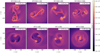 |
Fig. 1. Column density in the HYDRO runs (top row) and in the magnetic runs (bottom row) at low resolution (far-left panels), mid resolution (center left), high resolution (center right), and very-high resolution (far right panels). The column density is computed over 200 AU along the x-axis (the rotation axis) and is displayed in the x = 0 plane at the end of the runs. White dots indicate sink particle positions. Gas velocity vectors are overplotted. |
We aim to check whether a given spatial resolution allows for the observation of the spiral arm formation. In the hydrodynamical case, a 10 AU resolution is sufficient to capture structures prone to fragmentation, although circumstellar and circumbinary disks can be confused, and a 5 AU to 1.25 AU resolution appears to give a converged qualitative picture.
In all magnetic runs, a pseudo-disk is present. It is characterized by an enhanced density compared with the surrounding medium, a magnetic pressure dominating over thermal pressure, and infall motions. Its size increases with time. In Fig. 1, it is clearly visible in the MU2-MR and MU2-HR runs, with a ∼1000 AU radius, as well as in the MU2-VHR run, with a ∼700 AU radius. We do not focus on the pseudo-disks (Galli & Shu 1993) but rather on the rotationally supported disks in which the centrifugal acceleration ensures radial equilibrium (these are simply called “disks” for the rest of the paper). As can be seen in the bottom-left panel of Fig. 1, in run MU2-LR there is no rotating disk larger than the sink particle size at t = 10 kyr. Consequently, there is no spiral arm or filament connecting the two sinks or their surrounding accretion structures. In this run, disks appear after about half of the simulation time. In runs MU2-MR, MU2-HR, and MU2-VHR, we found individual disks, spiral arms, and a filament linking the two disks, just as in the hydrodynamical case. In run MU2-MR, individual disks were resolved, but over the integration time, we did not observe the formation of new spiral arms after a binary had formed. In contrast, we report that spiral arms kept forming regularly in runs MU2-HR and MU2-VHR, although they are hardly distinguishable in a single time snapshot such as Fig. 1. In run MU2-VHR, a third sink particle formed in one of the individual disks after spiral arm collision (reminiscent of Mignon-Risse et al. 2021b). The common accretion disk, where the third sink formed and is still embedded at the end of the run, is the closest structure to what could be called a circumbinary disk in any of these simulations.
For the magnetic case, under these conditions, we found that a spatial resolution of 2.5 AU is sufficient to resolve the structures prone to fragmentation, which does not mean that convergence is reached (see Sects. 3.2 and 3.3). In particular, disks (more easily identifiable by their column density structure than by rotation arguments; see Mignon-Risse et al. 2021b) are smaller than in the hydrodynamical case (see Sect. 4.4; and smaller than in Mignon-Risse et al. 2021b). Consequently, spiral arms and fragmentation induced by spiral arm collision appear at higher resolution than in hydrodynamical runs, and fragmentation might be missed in simulations that do not reach such spatial resolution requirements.
We note that the cavities visible in the bottom-left panel of Fig. 1 (run MU2-LR, also visible later in the other magnetic runs) are reminiscent of those reported in Hennebelle et al. (2020), Commerçon et al. (2022), and Mignon-Risse et al. (2021b). These are likely due to the interchange instability (see Appendix B of Mignon-Risse et al. 2021b).
3.2. Jeans length
After we addressed the spatial resolution needed to capture the structures of interest, we set out to see how resolution impacts the Jeans length. The (thermal) Jeans length is defined as
 (3)
(3)
where  is the local sound speed and with γ = 5/3 (in our calculations) as the adiabatic index. The magnetic Jeans length LJ, mag is defined in a similar fashion but using
  , where
  is the Alfvén speed, instead of cs (more details are given in Sect. 4 on the comparison between LJ and LJ, mag). For an alternative approach to computing the Jeans length in the MHD case, we refer the reader to the appendix of Myers et al. (2013), who also discuss the anisotropy of magnetic effects. We note, that the difference between the LJ, mag they derive and our simple formulation is minor.
Figure 2 shows the minimal Jeans length as a function of the maximal AMR level (a higher AMR level means a finer resolution by a factor of two). Hence, one would like the Jeans length slope to be less steep than a  slope and to ideally become flat, indicating that the Jeans length becomes increasingly well sampled as the resolution increases. It is visible in Fig. 2 that for certain AMR levels, the smallest Lj actually decreases faster than a
  slope. It is particularly visible from lmax = 13 to lmax = 14 (runs HYDRO-LR and HYDRO-MR). Indeed, we found that the maximal density reached increases with the resolution (not shown here for conciseness). Consequently, a higher maximum AMR level does not always result, in our simulations, in a better-sampled Jeans length. Nevertheless, we checked that the minimal Jeans number, that is, the number of cells sampling a Jeans length, is generally larger than eight at the maximum level so that artificial fragmentation is avoided (see the discussion in Sect. 5.1). There is no clear trend in the magnetic runs for a Jeans length generally decreasing less steeply than
  . Nevertheless, it is the case from lmax = 14 to lmax = 16 for the hydro runs, which corresponds to a resolution of 2.5 AU (run HYDRO-HR) to 1.25 AU (run HYDRO-VHR).
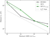 |
Fig. 2. Minimal Jeans length as a function of the maximal AMR level lmax computed at t = 10 kyr. A higher AMR level means a finer resolution. Each point refers to a simulation of Table 1. In the magnetic case, we computed the thermal (LJ, see Eq. (3)) and magnetic (LJ, mag) Jeans length. An additional AMR level gives a finer resolution by a factor of two. |
Finest spatial resolution and magnetization level of the different runs.
In summary, checking the Jeans length sampling at a given resolution only indicates that fragmentation, if reported, is not artificial (Truelove et al. 1997, see also Federrath et al. 2011 and the discussion in Sect. 5.1). It does not mean that the Jeans length converges toward a unique value because it depends on the density and temperature, which depend on the maximum resolution.
3.3. Multiplicity: Number of sink particles
Figure 3 shows the number of sinks as a function of time. We distinguish three phases: initial fragmentation (increasing number of sinks), due to Toomre-unstable disk fragmentation; mergers (number of sinks decreasing toward a value of 2); and secondary fragmentation. In runs HYDRO-VHR and MU2-VHR, only two sinks are formed after the first fragmentation phase, so there is no merger phase.
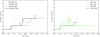 |
Fig. 3. Number of sink particles as a function of time in the HYDRO runs (left panel) and in the magnetic runs (right panel). |
In the figure, it can be seen that the sink multiplicity increases before t = 6 kyr from one (the initial sink) to a number between two and five. This is the initial fragmentation epoch, which is highly impacted by the formation of a disk with a density bump on top of it and prone to fragmentation, as it is the most Toomre-unstable region (see Paper I). This structure fragments rapidly (in less than one orbital period, Norman & Wilson 1978) into four pieces in runs HYDRO-LR and MU2-LR, and the process is likely triggered by the Cartesian grid. As mentioned in Paper I, these grid effects dominate when there are smooth initial conditions. Other possibilities to trigger the instability would be to choose perturbed (e.g., Commerçon et al. 2008; Kuruwita et al. 2017) or turbulent initial conditions (e.g., Gerrard et al. 2019; Kuruwita & Federrath 2019; Mignon-Risse et al. 2021b) to trigger the instability. In the other runs, we nevertheless observed the development of non-axisymmetries similar to spiral arms around the primary sink where additional sinks form. In runs MU2-MR, MU2-HR, and MU2-VHR, the disk is affected by magnetic forces and is elongated into a bar, which is similar to the structure reported in Machida et al. (2005a) following Machida et al. (2005b). Hence, in these cases, the disk instability has unlikely been triggered by the grid.
During a second phase, the sink multiplicity decreased as sinks merged. The central sink was initially in an unstable equilibrium, as it was surrounded by massive companions. Hence, any shift (e.g., caused by numerical errors or any asymmetry) led this sink to leave the center. We understand the drop in sink multiplicity to be due to gravitational interactions between sinks. Because of these interactions, the sinks’ angular momentum (computed with respect to the origin) changes, favoring the migration of some sinks toward the center, where the primary sink is initially located, until they merge. Eventually, all runs showed a binary system at some point between t = 7.5 kyr and t = 10 kyr.
In the hydrodynamical runs, the sink multiplicity increased again during the third phase, and we refer to this event as a secondary fragmentation. At this stage, each sink of the binary system had developed an accretion disk. New sinks formed at the extremity of spiral arms or following the collision between a spiral arm and a filament or another spiral arm. The final number of sinks was between four (mid, high, and very-high resolution) and seven (low resolution). According to the value of the Jeans number being larger than eight in the HYDRO-LR run and most fragmentation structures (circumbinary disk, filaments) being captured, fragmentation was physical rather than numerical. Nonetheless, the excess of sinks in run HYDRO-LR can be explained by the lack of convergence regarding the resolution of structures.
In the MU2 runs, the number of sinks at the end of the simulations was between two and three. In run MU2-LR, we showed in Sect. 3 that no clear disk structure forms around the two sinks (bottom-left panel of Fig. 1). Hence, we did not expect the formation of additional sinks, as this system had reached a quiescent state. As shown in run MU2-VHR (bottom-right panel of Fig. 1), secondary fragmentation is not fully prevented in the presence of magnetic fields, as we observed that a third sink particle had formed from spiral arms collision. It occurred in the close neighborhood of an existing sink, at a distance of 19 AU. This could not have occurred in run MU2-HR with such a small orbital separation because of the two sinks accretion radii (10 AU each).
Figure 4 shows the orbital separation between the sinks that will eventually become the two most massive sinks over time (see also Fig. 5). We found it to correctly converge with resolution. The evolution of the orbital separation is studied in more detail in Sect. 4.2.
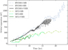 |
Fig. 4. Orbital separation between sinks #1 and #2 as a function of time. |
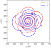 |
Fig. 5. Trajectory of sinks #1 and #2 in run HYDRO-HR in the yz-plane. This corresponds to the plane perpendicular to the initial rotation axis. The sinks location at t = 5 kyr, t = 10 kyr, and at the time of secondary fragmentation is indicated by the dots, the triangles, and the empty squares, respectively. |
Overall, we observed hierarchical fragmentation with each sink possessing its own disk that can lead to additional fragmentation in the hydrodynamical case as well as in the magnetic case. We find that early fragmentation is compensated by enhanced stellar mergers following gravitational interactions and radial migration. This suggests that high-multiplicity systems born from disk fragmentation likely formed out of hierarchical fragmentation rather than from a single disk.
3.4. Conversion of gas into stars
Figure 6 shows the sum of all sink masses as a function of time. We observed a satisfying convergence in the HYDRO run at the end of the simulation, within ≈20% with respect to the HYDRO-VHR run. We nevertheless observed large variations at low resolution (run HYDRO-LR). We recall that the density threshold for accretion obeys a scaling relation (Hennebelle et al. 2020), which appears here to lead to self-consistent results. In the magnetic runs, we found an agreement on the total mass within ≈20% as well as at the end of the runs. To sum up, the total mass is nearly independent of spatial resolution, especially at late times.
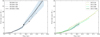 |
Fig. 6. Sums of all sink masses as a function of time. Left panel: sums of all sink masses in the HYDRO runs. The filled circles indicate the secondary formation epoch. Right panel: sums of all sink masses in the MU2 runs. In both panels, the blue region shows the value obtained in the highest resolution runs ±20%. |
4. Influence of magnetic fields
In this section, we investigate the role of magnetic fields. We focus first on the impact of magnetic fields on the fragmentation modes, then on the properties of massive multiple stellar systems.
4.1. Multiplicity and modes of fragmentation
We observed two common fragmentation mechanisms between hydrodynamical and magnetic cases, namely, Toomre-unstable disk fragmentation (with a transition through an elongated bar in high-resolution magnetic runs) and arm-arm collision. Moreover, in all runs we observed sink mergers and the presence of a binary system after the early fragmentation epoch (Fig. 3). However, the secondary fragmentation phase, reported in the hydrodynamical runs, does not exist in most of the magnetic runs except for a sink particle born out of spiral arm collision in run MU2-VHR, indicating that fragmentation is not totally suppressed by magnetic fields. Meanwhile, arm-filament collision, which is found to trigger fragmentation in the hydrodynamical runs, was not observed in any magnetic runs. Indeed, filaments linking binaries (as also observed by, e.g., Sadavoy et al. 2018 in IRAS 16293–2422) are more diffuse when magnetic fields are included, as can be seen in Fig. 1, which may be due to the additional magnetic pressure (as can be the case for larger-scale filaments; see e.g., Federrath & Klessen 2012; Gutiérrez-Vera et al. 2023) in regions of smaller density compared to the disks, where pressure support is mainly magnetic. By broadening the filaments, magnetic pressure prevents, indirectly, fragmentation induced by arm-filament collision.
As shown in Fig. 2, fragmentation is not directly suppressed by magnetic pressure support. As discussed, magnetic fields indirectly prevent the fragmentation through arm-filament collision, but magnetic pressure has a minor impact on the Jeans length. Indeed, we found that regions of small Jeans length are as numerous in the hydrodynamical cases as in the magnetic cases. Similarly, within the magnetic runs, the minimal Jeans length and magnetic Jeans length are roughly equal because thermal pressure largely dominates over magnetic pressure. Moreover, LJ and LJ, mag converge toward the same value at high resolution, while in run MU2-LR no thermally supported disks were formed at t = 10 kyr. When looking at the Jeans length more generally, we found that LJ and LJ, mag differ where the Jeans length is already large and therefore where the gas is already stable against fragmentation. Hence, magnetic pressure is not responsible for these differences in sink multiplicity. More than that, if the scales on which ambipolar diffusion is efficient are not sufficiently resolved, the magnetic field piles up, which leads to an overestimation of the stabilizing role of the magnetic pressure.
Overall, including magnetic fields in those simulations conserves two modes of fragmentation: Toomre-unstable disk fragmentation and fragmentation associated with arm-arm collision. However, we report no fragmentation induced by arm-filament collision in the magnetic case.
4.2. On the variations of the orbital separation in binaries
As shown in Fig. 4, the orbital separation between the stars that will become the most massive, a(t), is found to increase nearly linearly in all runs on timescales of ∼1 kyr. Quasi-periodic variations on timescales of the order of 1 kyr are linked to eccentricity (as in, e.g., Park et al. 2023). Variations on shorter timescales, for example between 15 kyr and 18 kyr in run HYDRO-VHR, are due to orbital motions with other companions born from secondary fragmentation. In the following sections, we study the impact of magnetic fields on the orbital separation and the two possible origins of the outspiral motion, gravitational torques from the gas and gas accretion.
To this end, we first present the equation describing the orbital separation evolution of the binary. Under the approximation of equal-mass binaries (which is the case most of the time in the hydro runs when two stars are present, as well as in the magnetic runs) and centrifugal equilibrium, we have a = 16j2/(GM), where j is the specific angular momentum of the binary and is also equal to the angular momentum of each component of the binary and where M is the total mass of the binary. Subsequently, the temporal variation of the orbital separation can be derived as
 (4)
(4)
so that the condition for an increasing orbital separation is
 (5)
(5)
The formulation is similar to (e.g., Tiede et al. 2020). When computing the evolution of the sinks angular momentum and mass over timescales of ∼1 kyr, on which we observe an increasing separation (Fig. 4), we find this condition to be met and to be physically consistent with the outspiral we observe.
4.2.1. Impact of magnetic fields on the separation
We investigate whether magnetic fields have any impact on the increasing separation. We observed that the orbital separation is reduced by a factor of two in binaries when magnetic fields are present. Since a(t) is nearly linear, it takes the form a(t) = αt where α is a constant, with αHYDRO ≈ 2αMU2. Hence, the quantity ȧ/a (where the dot indicates the time derivative) is equal in both cases. In other words, the orbital separation evolution is unaffected by magnetic fields.
Magnetic fields only interact with sinks via their effect on the gas. To address the possible angular momentum removal by magnetic braking, we computed the angular momentum at two distinct epochs on cubes encompassing the binary system. On the one hand, we focus on early times and small scales around the center of the cloud. When computing the angular momentum in a cube with a side of 800 AU centered onto the grid origin at 3.5 kyr (typically the time when the secondary sink forms), we find that the specific angular momentum is reduced by 30% in the magnetic case. Hence, by the time the secondary sink forms, part of the angular momentum has been removed by magnetic braking. This impact of magnetic fields explains the difference in the initial orbital separation of binaries.
On the other hand, we focus on later times, which means larger scales because the orbital separation increases. When computing it in a cube with a side of 2000 AU centered onto the grid origin at t = 5 kyr and 10 kyr, we did not find significant differences between the hydrodynamical runs and the magnetic runs. Hence, in the following paragraph we try to explain the lack of efficiency of the magnetic braking (with respect to the center of mass, which is the center of rotation in the system). This mechanism’s strength is proportional to the toroidal and poloidal components of the magnetic field, with the toroidal component developing from coherent (differential) rotation. Between t = 5 kyr and 10 kyr, each star has a disk but no circumbinary disk. The consequence of this is twofold: First, as illustrated in the top panel of Fig. 7, the magnetic field strength outside the individual disks is smaller (by a factor of a few times unity to a factor of approximately 100) because the density in such areas is smaller. Second, portions of the gas rotating coherently around the binary indeed generate a toroidal field. Locally, Bϕ/∥B∥ ≈ 1, as shown in the bottom panel of Fig. 7. However, these portions are too small, and the local magnetic field strength is also too small for the overall magnetic braking to slow down the rotating gas on timescales shorter than the time it takes for this same gas to reach either of the two individual disks. In the disks, the magnetic braking with respect to the center of mass is negligible, as expected. Hence, the binary system’s angular momentum cannot be transported efficiently by magnetic fields.
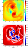 |
Fig. 7. Maps of B/B0 (top panel) and Bϕ/B (bottom panel) in the orbital plane in run MU2-HR at t = 10 kyr. In this case, B0 is the initial uniform magnetic field strength. Sink particles are denoted by white circles. |
Therefore, since ȧ/a is equal in both cases, this suggests that the value of a(t) is inherited from its initial value, which differs in the hydrodynamical cases and in the magnetic cases because of magnetic braking. Hence, magnetic fields reduce the initial separation but not its further evolution.
4.2.2. Gravitational torques contribution
Next, we discuss our investigation into the contribution from gravitational torques and gas accretion onto the increasing separation shown in Fig. 4. To probe the former, we computed the sink specific angular momentum j and the gravitational torques from the gas onto the sinks, noted as rgϕ, which accounts for the Plummer softening specific to gas-sink interactions. The specific angular momentum increased globally with time, with values of the order of 1018 cm2 s−1 and a slope of ≳106 cm2 s−1. This is expected because the orbital separation increases with time, whereas the binary mass, which can only increase, promotes orbital shrinking. Theoretically, the gravitational torque must be negative when corresponding to the disk part lagging behind a sink and positive when it is in front of it (see e.g., Tiede et al. 2020). If the gas distribution was perfectly symmetric with respect to the binary axis, the sum of the two torques should be zero. Meanwhile, spiral arms, companions (when present), and low-density cavities caused by the interchange instability (in the magnetic models) should make this total torque deviate from zero. This is supported by our results: The total gravitational torque, rgϕ, shown in Fig. 8 for runs HYDRO-HR and MU2-HR starts showing oscillatory-like behavior at about the orbital period, which is when spiral arms develop and a companion forms (in the hydro runs). This behaviour is caused by those spiral arms, then the companion orbiting around the star and alternatively contribute to a positive and negative torque. Notably, low-density cavities always lag behind the sinks, and their presence should translate into a positive torque on the sinks since we found the torque to oscillate around zero. This contribution appears to be negligible compared to the spiral arm contribution. We note, however, that the oscillation amplitude is larger in the magnetic runs than in the hydro runs. This is likely due to the disks being smaller in the magnetic case, as the distance to the entire spiral arm structure is smaller and the associated gravitational torque, which decreases quadratically with the distance, is larger. Overall, the envelope of the oscillations in rgϕ has an amplitude of ≈105 cm2 s2. This is one order of magnitude too small to explain the slope of the specific angular momentum evolution. Hence, only gas accretion can explain the increasing orbital separation.
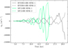 |
Fig. 8. Gravitational torque rgϕ acting on binaries in runs HYDRO-HR and MU2-HR as a function of time. |
4.2.3. Gas accretion
As shown in Eq. (5), gas accretion, depending on its specific angular momentum and mass, can contribute to either increasing or decreasing the separation. However, in those simulations the general trend is an increasing separation. It is therefore critical to understand why this occurs and to see whether it is purely linked to our setup.
After integrating both sides of Eq. (5), we obtained dj/j > dM/2M. Then, we integrated the left-hand side from j0 to j′ and the right-hand side from M0 to M′, where j0 (j′) is the sink specific angular momentum prior to (after) accretion, and M0 (M′) is the sink mass prior to (after) accretion, yielding  . To go further, we expressed j′ and M′ as functions of j0, M0, as
 (6)
(6)
where we labeled the accreted gas angular momentum jgas and the accreted mass Mgas, and used M′=Mgas + M0, which we replaced in the previous inequality. After some simple algebra, we found that as long as the gas mass increment is negligible compared to the sink mass (Mgas ≪ M0) we could neglect second-order terms (Mgas/M0)2. This led to the following criterion for an increasing orbital separation:
 (7)
(7)
where  from radial equilibrium between the sinks. The previous inequality is a reformulation of the trend found in the pioneering studies of Bate & Bonnell (1997), Bate (2000). Putting in typical values of separation and binary mass from the simulations, we found that gas accretion increases the separation of the binary if
 (8)
(8)
We use the fiducial values in Eq. (8) in order to investigate whether the gas, initially located at a given radius and with a given angular momentum (somewhat arbitrary in the present set of simulations), possess enough angular momentum to fulfill the condition in Eq. (8) and therefore increase the orbital separation of the binary at the time of interest. For our initial rotation profile, the fiducial value of Eq. (8) corresponds to the gas initially located at radii > 103 AU. We then examined a follow-up issue to ensure the validity of the reasoning, that is, whether the gas initially located at this radius has enough time to reach the binary. We determined that based on its associated free-fall time, the gas does have enough time to do so. The scenario of an orbital separation driven by gas accretion in our simulations was therefore shown to be consistent.
The next natural element to determine was how this value depends on the initial profile. For different initial rotation profiles, such as the slow and fast models presented in Commerçon et al. (2022), the gas should be initially located at ∼104 AU in order to drive the outspiral of such a binary. We note, however, that our comparison should be taken with caution because a different rotation profile would likely result in a distinct evolution of the system (e.g., Bate 2000).
To summarize this subsection dedicated to the orbital separation evolution, we found that gas accretion is mainly responsible for the binary outspiral, and we can link such a trend to the initial rotation profile of the core. We observed the influence of magnetic fields in only one aspect: they remove the angular momentum in the innermost regions of the cloud at early times, setting a smaller initial orbital separation for binaries than in the hydrodynamical case. However, the magnetic fields play no significant role in the subsequent evolution of the orbital separation.
4.3. Conversion of gas into stars
As visible in Fig. 6, in the hydrodynamical case, the total mass of all sinks is ∼30 M⊙ near the end of the simulation (t = 17.5 kyr), compared to ∼15 M⊙ in the magnetic case. Nonetheless, the mass growth is similar in both cases within 30% up to ∼10 kyr.
In the magnetic case, the mass increases with a mean accretion rate slightly smaller than 10−3 M⊙ yr−1. In the hydrodynamical case, the mean accretion rate is at Ṁ ≈ 10−3 M⊙ yr−1 up to the secondary fragmentation epoch (indicated by the circles in Fig. 6). After that point, it is Ṁ ≈ 3.5 × 10⁻³ M⊙ yr−1. Hence, the change in the mean accretion rate occurs just before secondary fragmentation. This is consistent with the fragmentation being linked to spiral arms. Indeed, the spiral arms carry angular momentum outwards, allowing the central object to accrete. Though, this argument does not explain why the accretion rate remains at a higher value. A possible explanation could be the initial density profile ρ(r)∝r−1.5 making more gas available for accretion at later times. However, this would not explain the difference between the hydrodynamical case and the magnetic case. Moreover, this trend is not observed in Paper I during the run with a single sink (neither in the study of Oliva & Kuiper 2020 with a similar initial density profile). Hence, we do not attribute the enhanced accretion to the initial density profile. Another possibility is that the presence of new close (∼100 AU) companions also triggers the formation of spiral arms on shorter timescales (the orbital timescale between the two close components), encouraging accretion. Similarly, the sinks born during secondary fragmentation form their own disks, which have their own spiral arms. A disk and a sink can perturb the secondary disk via their spiral arms and tidal forces, respectively (see e.g., Savonije et al. 1994), and as a consequence, the secondary disk grows spiral arms and accretion becomes enhanced.
In the following paragraphs, we investigate the role of sink multiplicity on the accretion rate using Fig. 9, which shows the instantaneous accretion rate as a function of time, and look for patterns. In the magnetic case, and in particular for run MU2-HR, we observed accretion peak-like features after 10 kyr that could be periodic. We extracted the exact time of the features by selecting the time of accretion rates that correspond to the local maxima and that are greater than the mean accretion rate in the simulation. We found that the time between two maxima is between 0.75 kyr and 1.0 kyr. This interval matches the semi-orbital period that can be extracted from the sink motions (also visible in the orbital separation plot, Fig. 4, thanks to the nonzero eccentricity of the system). This result is consistent with the m = 2 mode expected to develop when the binaries are not too close, for which the spiral wave pattern speed is the orbital frequency (Savonije et al. 1994). In order to check for this periodicity, we computed the Fourier power spectrum of the accretion rate after 10 kyr, as shown in Fig. 10. We found an enhanced signal at frequencies between 0.7Ωorb and 2Ωorb. In particular, we found no significant periodicity above 2Ωorb. Nonetheless, it is difficult to draw firm conclusions from Fig. 10 even though it suggests a plausible periodicity in the signal. Indeed, we know that the system’s orbital frequency is not constant with time, and there may be a non-periodic part of the signal that is not strictly constant either (see Fig. 9). Moreover, only a few (approximately three) orbital periods were captured after 10 kyr within the simulation time. This shows, however, that a link between multiplicity and the accretion rate is plausible and not only justified theoretically.
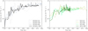 |
Fig. 9. Accretion rates as a function of time. Left panel: accretion rates in the HYDRO runs. The filled circles indicate the secondary formation epoch. Right panel: accretion rates in the MU2 runs. |
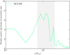 |
Fig. 10. Fourier power spectrum of the accretion rate in run MU2-HR after 10 kyr. The x-axis is the Fourier transform frequency normalized by the approximated orbital frequency Ω = 1/2.5 kyr−1. Data (instantaneous accretion rates) were linearly interpolated in order to have a uniformly spaced sample to perform the fast Fourier transform. The gray band indicates the 0.7 − 2Ωorb interval. |
In the hydrodynamical runs, we found that the timescale between such accretion peaks mainly lies in the 0.1 − 0.4 kyr interval. This is also consistent with the previous scenario since a larger (greater than two) sink multiplicity involves more than one characteristic frequency, and in those runs there are also close binary systems with higher orbital frequencies than in the magnetic runs. Because there are several frequencies involved, the periodicity in the accretion rate is more difficult to extract and much less visible (Fig. 9).
Our simulations did not show a direct influence of magnetic effects on the accretion rate. However, they suggest a possible modulation of the accretion rate at the orbital period due to the gravitational influence of a companion. Nevertheless, the system on hand is not well suited to extract such quasi-periodic features, as it has more than two components, a variable orbital period with time, and a binary embedded in a collapsing core.
4.4. Individual disk radius
In this section, our aim is to estimate the radius of the individual disks surrounding sink particles, to reveal the underlying process regulating its size, and to emphasize the differences observed between hydrodynamical and magnetic models. Several diagnostics can be used, in principle, to derive the radius of a disk.
First, we considered using kinematic signatures, as is done observationally with velocity-position diagrams (e.g. Murillo et al. 2013; Tobin et al. 2020). One way to do so in the simulation is to compute the deviation with respect to Keplerianity (as done in Paper I) on a cell-by-cell basis and to reduce this information to a single scalar by computing the mean or median azimuthal value and looking for a transition radius. However, we found the Keplerianity to vary significantly between the cells, as it is greatly affected by the stellar companions. The same limitation was encountered when using the disk criteria presented in Joos et al. (2012) and used, for example, in Mignon-Risse et al. (2020). Therefore, we chose not to focus on a kinematic definition of the disk, although our results still point to structures dominated by rotation.
Observationally, dust continuum fitting is used as an alternative to kinematic signatures of disks (e.g., Patel et al. 2005). As in Mignon-Risse et al. (2021b), we decided to use the surface density as a criterion to define the disk and, thus, the disk radius. Upon integrating the surface density over a depth of 200 AU perpendicular to the disk plane (we note that this is already sufficiently larger than the typical disk height of less than 50 AU), we obtained the surface density Σ(y, z), which is a two-dimensional function, as it depends on the spatial coordinates in the disk plane. The largest surface density was found to be around Σ ∼ 1026 cm−2, decreasing to Σ ∼ 1023 cm−2 at cylindrical radii of 400 AU. We reduced Σ(y, z) to a 1D function by computing its azimuthal median, taking one sink’s location as the coordinates’ origin, and we obtained Σmedian(rcyl). We used a threshold criterion to identify the disk radius as the cylindrical radius within which the surface density Σmedian(rcyl) exceeds a critical value that is taken to be 1025 cm−2. Using this diagnostic, we found that the disk grows in size, reaching 100 to 150 AU size in hydrodynamical runs before secondary fragmentation. After secondary fragmentation, during which the newly formed companion starts forming its own disk, the primary disk radius decreases and remains between 60 AU and 100 AU in runs HYDRO-HR and HYDRO-VHR. During this epoch, the companion gains mass rapidly, and the disk radius is compatible with disk truncation, predicted to be about 0.3 of the orbital separation (Papaloizou & Pringle 1977; Paczynski 1977). Meanwhile, in the magnetic runs, the disk radius remains generally smaller than 100 AU even though no companion forms, as shown in Fig. 11, and is compatible with magnetic regulation (Hennebelle et al. 2016). Varying the threshold value to 5 × 1025 cm−2 decreased the obtained disk radius by about 20 AU.
 |
Fig. 11. Disk radius as a function of time. It is computed from the surface density with a threshold value N = 1025 cm−2 (black curve), N = 5 × 1025 cm−2 (gray curve), and the plasma β (green curve) in run MU2-VHR and with the plasma β in run MU2-HR (green dashed curve). |
Finally, Commerçon et al. (2022) found that the protostellar disks formed in presence of ambipolar diffusion have β = P/Pmag > 1, where Pmag = B2/(8π) is the magnetic pressure. More recently, this has been shown in simulations incorporating Ohmic dissipation instead of ambipolar diffusion as well (Oliva & Kuiper 2023b). Following the former study, Mignon-Risse et al. (2021b) argued that this could serve as a way to measure the disk radius, especially when the dynamics and multiple stellar components make the comparisons between rotation profiles and Keplerian profiles difficult, which is the case here. In this work, we indeed found that the closest region to the sinks have a β > 1 and that the transition with β < 1 is located near the surface density transition setting the disk edge. With a spatial resolution smaller than 5 AU, we derived a disk radius, based on the plasma β, of 50 AU to 80 AU (see Fig. 11). This disk radius value is comparable to the surface density estimation using the largest surface density threshold among the two values explored in this study and is nearly constant when varying the resolution.
To conclude, we found the column density map and the plasma β to give a relatively compatible (±20 AU, depending on the surface density) and converged (for resolution finer than 5 AU) estimate of the disk radius. Disks are roughly two times smaller in the magnetized case compared to the hydrodynamical case before secondary fragmentation. They are compatible with magnetic regulation, while in the hydrodynamical case, they grow until fragmentation occurs and the newly formed companion truncates the primary disk. Hence, in the hydrodynamical case, this result could be interpreted as the disk size not being regulated (i.e., it gathers material reaching its centrifugal limit) or being regulated by fragmentation.
5. Discussion
5.1. Comparison with previous works
In the simulations we present, the refinement criterion for the AMR levels below the maximum is a Jeans length resolved by 12 cells. While in the original work of Truelove et al. (1997), a number of four cells was mentioned (and widely used since then, e.g., Kuruwita et al. 2017; Gerrard et al. 2019; other authors opted for eight cells, e.g., Masson et al. 2016; Rosen et al. 2016). To achieve convergence with smoothed particle hydrodynamics (SPH) methods, Commerçon et al. (2008) showed that in the hydrodynamical case, the Jeans length should be sampled by at least 15 cells. In order to resolve minimal dynamo amplification in self-gravity MHD simulations, Federrath et al. (2011) showed that 30 cells per Jeans length were required. Because the present initial conditions are not turbulent and the present disks do not develop turbulent states, we chose to keep the Jeans length resolution to 12 cells in order to save on computational time.
Bate (2018) studied the morphology of protostellar disks from molecular cloud simulations with SPH methods, neglecting magnetic fields. In our high-resolution hydrodynamical simulations (i.e., HYDRO-VHR), we obtained a quadruple system that is somehow similar to the one the authors depicted in their Fig. 4 (sinks 41, 89, 76, 83; see also Sigalotti et al. 2018). The systems have in common the following properties. They are both a point-symmetric system composed of two tight pairs surrounded by gas. Additionally, the two pairs are linked together by gas filaments continuously fed by the spiral arms belonging to protostellar disks. However, the authors report circumbinary disks around the tight pairs, while we do not. Instead, we found each star in the quadruple system to have a protostellar disk around it. This could be a matter of angular momentum budget of the surrounding gas since high angular momentum material is more prone to form circumbinary disks (Bate & Bonnell 1997). Finally, in our simulations, the youngest sinks formed from the interaction between the spiral arm belonging to the disks of the oldest sinks and the filament linking them. Such fragmentation triggered by arm-filament collision seems to occur in the authors’ study as well. We find, however, that the inclusion of magnetic effects suppresses this fragmentation mode, as magnetic pressure reduces the density contrast around the filament.
In this study, non-ideal MHD was included in the form of ambipolar diffusion. We therefore compare the properties of the multiple stellar systems formed in the magnetized runs with those of the binary systems reported in Mignon-Risse et al. (2021b), as the included physics are identical. The initial conditions are quantitatively different (e.g., core mass, rotation), and the qualitative difference comes from the inclusion of initial velocity dispersion to mimic turbulence, while in our work all the angular momentum originates from differential rotation. Unlike Mignon-Risse et al. (2021b), where a circumbinary structure is present under a particular turbulence level and magnetic field strength, except for the run MU2-VHR where a sink still orbited within the accretion disk it was born in, we found no circumbinary structure in the binary systems formed in our work. As in Mignon-Risse et al. (2021b), we did find mass ratios of the order of unity in binary systems. This fits the “high angular momentum core” case, while a “low angular momentum core” is predicted to result in unequal-mass binaries by Bate (1997), Bate & Bonnell (1997). The triple system in run MU2-VHR has masses 3.7 M⊙, 3 M⊙, and 1.4 M⊙ at the end of the run. Before the third sink formed, the binary system had a mass ratio close to one.
Preliminary works in low-mass star formation with ambipolar diffusion reported disk sizes reduced with respect to the standard hydrodynamical case (Masson et al. 2016; Hennebelle et al. 2016). As in the studies of massive isolated collapse by Commerçon et al. (2022), who report a single-star system, and Mignon-Risse et al. (2021b), where a binary system forms when initial turbulence dominates over magnetic fields, we found disks to be smaller in the non-ideal MHD case than in the hydrodynamical case based on the column density maps (and on the plasma β in the magnetic case). Recently, Lebreuilly et al. (2021) confirmed this trend on large samples in the context of collapses within massive (1000 M⊙) clumps, focusing their study on the population of protoplanetary disks, although their work was mainly oriented toward low-mass star formation.
Gerrard et al. (2019) studied the influence of an initialized turbulent magnetic field on disk fragmentation and outflow launching during the collapse of a low-mass pre-stellar core under the ideal MHD approximation. They claim that a turbulent magnetic field leads to a more isotropic magnetic pressure distribution when compared to a non-turbulent magnetic field and results in a reduced magnetic pressure gradient and more disk fragmentation. In fact, it can be expected from their assumptions (ideal MHD) that their disks are supported by magnetic pressure. In contrast, the disks formed in our work, in the presence of ambipolar diffusion, are thermally supported, so changes in the magnetic pressure distribution should not have a major influence on the disk fragmentation.
Magnetic fields may also play a role in the orbital separation of binaries. Recently, Harada et al. (2021) reported a numerical and analytical study of the impact of magnetic braking on massive close binaries in the ideal MHD framework. They show that the orbital separation is larger in the hydrodynamical case than when magnetic fields are introduced (their Eq. (6) with the non-specific angular momentum is equivalent to Eq. (5) in this work) because of magnetic braking and outflows. Our findings qualitatively agree with this result (see Fig. 4), as we find an orbital separation reduced by a factor of approximately two when magnetic fields are present. However, we attribute it to the initial separation being smaller because of early magnetic braking (when both stars were part of a coherent structure), while the further evolution of ȧ/a is comparable. Nonetheless, their results only apply to the further evolution of ȧ/a since the initial separation is fixed. Moreover, quantitatively, we also find orbital separations larger than 100 AU in the magnetic case, while they did not. Our results differ because the authors assumed a circumbinary structure able to extract angular momentum from the close binary, while we witnessed the formation of two separate disks, except in the secondary-fragmentation formed binary system of run MU2-VHR. Such differences are partially attributed to the different choices of initial mass and angular momentum budget, which, as we have shown, drive the evolution of the orbital separation in binaries formed from initial fragmentation. Our initial conditions are indeed different (i.e., magnetic field strength, mass, and angular momentum budget). The MHD version is different as well, as it is non-ideal in our work and ideal in their work. Ideal MHD has been found to overestimate the magnetic field strength in the densest (ρ ≳ 10−15 g cm−3) regions (Masson et al. 2016), impacting both disk formation and outflows (Commerçon et al. 2022). Nevertheless, our study supports the interpretation of Harada et al. (2021) that magnetic fields, in the form of magnetic braking, could play a prominent role in the formation of massive close binaries – on the condition of a coherent rotation structure, such as a circumbinary disk, at least initially. Further in time, however, gas accretion equally widens binaries in the hydrodynamical and magnetized cases in the absence of a circumbinary accretion structure.
The formation of a circumbinary disk structure around a low-mass protobinary system in non-turbulent and turbulent cores has been studied by Kuruwita & Federrath (2019) using simulations including ideal MHD. They report orbital shrinkage and attribute it to magnetic braking on the infalling gas. Alternatively, this event could be due to the sinks not being at centrifugal equilibrium when they form since they arise from initial perturbations and shrink their separation until they reach a stable orbit. To understand whether the final evolution of the binary orbital separation is consistent with gas accretion (that is, there is no outspiral), we put into Eq. (8) the final mass (∼0.5 M⊙) and the orbital separation (∼20 AU) of the protobinary system formed in the non-turbulent run of their study. This calculation gave a minimum gas angular momentum of 2 × 1020 cm2 s−1 to drive the binary outspiral through gas accretion; meanwhile, the protostellar core in their simulation has a maximal specific angular momentum of ≈1018 cm2 s−1 at the core edge. Hence, their pre-stellar core angular momentum budget is insufficient to drive the binary’s outspiral. Because they consider relatively small turbulent velocities (0.02 km s−1 and 0.04 km s−1), the angular momentum carried out by turbulence is still insufficient to drive the binary’s outspiral, and this naturally results in a similar final orbital separation in the non-turbulent and turbulent runs of the work of Kuruwita & Federrath (2019). Finally, in contrast to their turbulent runs, we did not report any circumbinary disk formation other than the one in run MU2-VHR where a companion had previously formed. This discrepancy could be due to the large (> 100 AU) orbital separation in our runs compared to theirs (∼20 AU).
We have investigated the impact of multiplicity on the accretion rate, whose understanding is missing in the star formation context. Indeed, it is not a free parameter but rather an outcome of the self-consistent collapse, even in the studies dedicated to multiple system formation (e.g., Harada et al. 2021). Nonetheless, the accretion rate in binaries has been investigated for binary compact objects (see e.g., Bowen et al. 2018), which are already introduced in the initial conditions. Periodicities in the accretion rate, such as those we investigate in Sect. 4.3, have been reported by Bowen et al. (2018), but those periodicities are dominated by the periodic inflow from circumbinary disks. Our present work suggests that no circumbinary disk is needed to modulate the accretion rate at orbital-like frequencies. This is in line with the episodes of enhanced accretion at periastron passage reported in Kuruwita & Federrath (2019).
Finally, we highlight the differences between this work and Paper I in terms of multiplicity and disk radius. First, we showed in Paper I that the multiplicity outcome of the system is sensitive to numerical choices, such as the sink properties (number, possibility to merge), and the numerical grid, as it can trigger instabilities that lead to fragmentation. In this work, we have chosen a numerical setup favoring multiple system formation in order to study the influence of magnetic fields on its properties. The approach is somehow similar to Bate (1997), except that in our case, the sinks formed self-consistently (within the uncertainty related to numerical choices as explained above). We checked whether the absence of an initial sink particle also leads to a binary system after a few ∼1 kyr, on which our analysis is performed, as well as to qualitatively similar results, which strengthens the results obtained in this work. Indeed, as presented in Sect. 3.3, mergers are triggered when the multiplicity is higher than two in the innermost region of the cloud. For a higher multiplicity to be reached, hierarchical fragmentation is necessary in the present simulations. This study also illustrates how fragmentation, even with an initial central sink particle, leads to symmetry breaking with respect to the axisymmetric initial conditions. Allowing the central sink particle to move is key, in the present study, in order to avoid enforcing the central symmetry. The present results on the orbital separation also bring additional clues to the debate regarding the link between the early phases and the multiplicity outcome. Indeed, this link between early phase central fragmentation and the ultimate fate of the system is due to the orbital separation increasing since it brings stars apart into the form of a multiple system. We show here that such a trend depends on the initial angular momentum and mass distribution of the cloud because the outspiral is driven by gas accretion. Second, we note that the single disk in Paper I is larger than the disks formed in the binary systems of the HYDRO runs. In these runs exhibiting a binary system (and in the magnetic runs as well), the disk radius is smaller than the tidal truncation radius, which is approximately 0.3 times the orbital separation for equal-mass binaries (Papaloizou & Pringle 1977; Paczynski 1977). Hence, the disk radius is not attributable to tidal truncation by the companion before the secondary fragmentation epoch. This occurrence is most likely due to hierarchical fragmentation in which the specific angular momentum of the fragments is smaller than that of the parent cloud. Hierarchical fragmentation was already mentioned as a possible solution to the angular momentum problem in star formation (see e.g., Bodenheimer 1978; Zinnecker 1984). After secondary fragmentation, however, as the multiplicity becomes larger than two, the disks are most likely truncated by tidal forces as they extend from one sink to the companion’s disk (e.g., this is particularly visible for the HYDRO-HR and HYDRO-VHR runs in Fig. 1).
5.2. Comparison with observations
The initial specific angular momentum profile j ∝ R1.25 (see Sect. 2.2), where we recall that R is the cylindrical radius, is motivated by theoretical purposes (Meyer et al. 2018, 2019). It may not be representative of typical cores if such massive pre-stellar cores do exist (see e.g., Zhang et al. 2020 for candidates and Tan et al. 2014; Motte et al. 2018 for recent reviews). For instance, (Pineda et al. 2019) measured j ∝ r1.8 in low-mass dense cores, which is not so different from the measurements of Goodman et al. (1993), who found a specific total angular momentum J/M ∝ r1.6 (the slope of j and J/M are the same for monotonic profiles; see Pineda et al. 2019). Meanwhile, the core (or more generally, infalling gas) properties could be important in setting the angular momentum versus mass budget and therefore the evolution of the orbital separation of binaries, as studied in Sect. 4.2. Nevertheless, this reasoning relies on a high-mass star formation process similar to that of low-mass stars. Large-scale dynamics, such as hierarchical collapse, should be taken into account, but this is beyond the scope of this paper.
We find that with and without magnetic fields, primary disks form and fragment, and the fragments eventually possess their own disks as well. This hierarchical picture for fragmentation is supported by the recent observations of Suri et al. (2021) in AFGL 2591. Furthermore, the multiplicity of outflows in AFGL 2591 has been used by Gieser et al. (2019) to infer the presence of fragmented cores. Even though outflows are not the main topic of the present paper, we note that we did find magnetic outflows, just as we did in Mignon-Risse et al. (2021a), launched from individual objects in multiple systems (here represented as sink particles) while core collapse was still ongoing. This evidence confirms magnetic outflows (namely, magnetic tower flows and magneto-centrifugal outflows, as studied in Mignon-Risse et al. 2021a) as relevant candidates for the protostellar outflows observed in multiple protostellar systems. However, we note that the comparison of polarized emission maps produced in the outflow region with the observations is beyond the scope of this paper.
As already reported in Mignon-Risse et al. (2021b), we found a prominent role of spiral arms in the formation of (massive) multiple stellar systems. Interestingly, Tobin et al. (2016) found evidence that the triple protostellar system L1448 IRS3B is still embedded in the spiral arms it may have formed from. This is consistent with the present picture if low- and high-mass multiple stellar systems share similarities in their accretion process.
We note that we do not report runaway stars in any of the present simulations. In the HYDRO runs (of all resolutions) and the MU2-VHR run, the multiplicity was strictly larger than two, so N-body interactions could possibly eject stars if the computation was integrated for a longer time. Further work is needed to reconcile massive star formation simulations with the high frequency of the massive runaway stars reported by observations (see e.g., Dorigo Jones et al. 2020 and references therein).
A large fraction of massive stars are in close binaries (e.g., Sana et al. 2012). While dynamical interactions have been shown to be a relevant process to forming close (< 10 AU) binaries (Bate et al. 2002), our run MU2-VHR shows that disk fragmentation of magnetized disks could be a possible pathway. Indeed, we found an initial orbital separation of 19 AU (which remained nearly constant for the short integrated time, namely, 16 AU after 1.7 kyr) and a common accretion structure. For a possible orbital shrinking to be followed, we would need a finer resolution (in run MU2-VHR, 5 AU is the sink radius). We leave this to further work.
In contrast, an excess of “twin” (mass ratio between 0.95 and 1) low-mass binaries with orbital separations greater than 1000 AU have been reported in El-Badry et al. (2019) using the Gaia DR2 catalog. This population is unlikely to arise from close binaries widened by positive torques from a circumbinary disk since no circumbinary disk that large has ever been observed, so far. This observational result is in agreement with the non-magnetized large-scale numerical simulations of Bate (2018). While our results should be scaled down to low-mass binaries with care, they support gas accretion as a plausible candidate mechanism that helps form such a population after an initial fragmentation phase that could occur within the innermost region of the pre-stellar core. Indeed, we find gas accretion to widen binaries from a few tens of AU to 500 AU in the magnetized case with no sign of decrease and with an explicit criterion for further widening (see Eq. (8)).
6. Conclusions
In this paper, we have investigated the influence of both spatial resolution and magnetic fields on disk fragmentation and on the subsequent formation of massive multiple stellar systems. We considered eight runs with no restriction on the number of sink particles to be formed and with one sink already present at the center of the pre-stellar core. We studied the properties of the multiple stellar systems by varying the resolution and the presence of magnetic fields. At early stages, a density bump-like structure formed after the adiabatic stage and fragmented into several sink particles, breaking the axisymmetry via Toomre instability. The sink initially present interacted gravitationally with the other sinks and left the center of the cloud. When more than two sinks were present, their gravitational interactions induced radial migration with respect to the center of the cloud. The sinks gaining (losing) angular momentum migrated to larger (smaller) distances from the center until mergers occurred with the other sinks and the multiplicity reduced to two in all runs. The orbital separation in binaries increased as they accreted gas possessing angular momentum with respect to the center of mass of the binary (e.g., the center of the cloud). The separation decreased by a factor of two when magnetic fields were included, an effect caused by their initial orbital separation being reduced via magnetic braking. Hence, magnetic fields provide a promising method to explain the formation of close binaries if there is a common accretion structure.
The increasing orbital separation is driven by accretion of sufficiently high angular momentum gas. Such a trend in the orbital separation is likely to depend on the initial rotation profile. For initial conditions promoting a gas-driven outspiral, any fragmentation occurring in the early phases is crucial for the final fate of the system, as briefly presented in Paper I.
A second generation of stars formed from disk fragmentation around the first generation of stars. Such fragmentation can be triggered via arm-arm collision or arm-filament collision. In the magnetic case, arm-filament collision is absent. Our results are consistent with a hierarchical picture of fragmentation in the hydrodynamical case and in the magnetic case (as in, e.g., Park et al. 2023). We show that a resolution of 5 AU gives a converged picture in the hydrodynamical case, with the same occurring at a 2.5 AU resolution in the magnetic case. This spatial resolution corresponds to about 1/20 of the disk size, in order to resolve structures prone to fragmentation (filaments and spiral arms). Those values depend on the size of the first generation’s disks, which we found to be about two times smaller in the magnetic runs as compared to the hydrodynamical runs, before secondary fragmentation. We only observed secondary fragmentation in the magnetic case for a resolution of 1.25 AU, suggesting that a lack of fragmentation could be, in this particular case, due to a lack of resolution. These results will serve as references for future numerical studies. In contrast, based on the disk sizes we found, we conclude that any resolution above ∼100 AU simply lacks disk fragmentation.
Even at low resolution (10 AU in our case), the convergence regarding the total sink mass (15%) and the orbital separation of binary systems is correct. In the accretion rates of binaries, we found hints of modulations at the orbital frequency. This suggests that their tidal forces help the accretion onto the other object. If confirmed by further work, it means that fragmentation does not limit the mass of stars but rather enhances accretion bursts and possibly increases the efficiency of gas conversion into stars in multiple systems. Such confirmation would be of particular interest since massive stars are more often in multiple systems, as compared to low-mass stars (e.g., Chini et al. 2012). This moderates the argument of the fragmentation-induced starvation scenario (Peters et al. 2010) in which fragmentation reduces the maximal stellar mass by sub-dividing the mass reservoir into several lower-mass stars.
Overall, this work suggests that the influence of magnetic fields in the formation of multiple mass stars – without even focusing on the outflows, which are now understood as mainly magnetic – is important in several aspects. We find that magnetic fields regulate the disk size, which otherwise appears to only be regulated through disk fragmentation producing a companion and tidal truncation, by the same companion. Among the possible fragmentation modes (arm-arm collision, arm-filament collision), we find the arm-filament collision mode to be suppressed because the filaments are more diffuse in the presence of magnetic fields. Finally, magnetic braking reduces the orbital separation of binaries by a factor of two because (i) it reduces their initial separation and (ii) it has no impact on the further evolution of the orbital separation driven through accretion. In the absence of a common accretion structure, magnetic effects are insufficient to form close binaries. Regarding their strong impact on disk growth and fragmentation and on the initial orbital separation, we conclude that magnetic fields are important in the formation of multiple massive stars.
Acknowledgments
R.M.R. thanks A. Oliva and R. Kuiper for useful discussion. This work was supported by the CNRS “Programme National de Physique Stellaire” (PNPS). This work has received funding from the French Agence Nationale de la Recherche (ANR) through the project COSMHIC (ANR-20-CE31-0009). The numerical simulations we have presented in this paper were produced on the CEA machine Alfvén and using HPC resources from GENCI-CINES (Grant A0080407247). The visualisation of RAMSES data has been done with the OSYRIS (https://github.com/nvaytet/osyris) python package, for which R.M.R. thanks Neil Vaytet.
References
- Adams, F. C., Ruden, S. P., & Shu, F. H. 1989, ApJ, 347, 959 [Google Scholar]
- Ali, A. A., & Harries, T. J. 2019, MNRAS, 487, 4890 [NASA ADS] [CrossRef] [Google Scholar]
- Alves, F. O., Girart, J. M., Caselli, P., et al. 2017, A&A, 603, L3 [NASA ADS] [CrossRef] [EDP Sciences] [Google Scholar]
- Alves, F. O., Girart, J. M., Padovani, M., et al. 2018, A&A, 616, A56 [NASA ADS] [CrossRef] [EDP Sciences] [Google Scholar]
- Añez-López, N., Busquet, G., Koch, P. M., et al. 2020, A&A, 644, A52 [NASA ADS] [CrossRef] [EDP Sciences] [Google Scholar]
- Bate, M. R. 1997, MNRAS, 285, 16 [NASA ADS] [CrossRef] [Google Scholar]
- Bate, M. R. 2000, MNRAS, 314, 33 [Google Scholar]
- Bate, M. R. 2018, MNRAS, 475, 5618 [Google Scholar]
- Bate, M. R., & Bonnell, I. A. 1997, MNRAS, 285, 33 [NASA ADS] [CrossRef] [Google Scholar]
- Bate, M. R., Bonnell, I. A., & Bromm, V. 2002, MNRAS, 336, 705 [Google Scholar]
- Berthoud, F., Bzeznik, B., Gibelin, N., et al. 2020, Estimation de l’empreinte carbone d’une heure.coeur de calcul, https://hal.archives-ouvertes.fr/hal-02549565 [Google Scholar]
- Beuther, H., Soler, J. D., Linz, H., et al. 2020, ApJ, 904, 168 [NASA ADS] [CrossRef] [Google Scholar]
- Bleuler, A., & Teyssier, R. 2014, MNRAS, 445, 4015 [Google Scholar]
- Bodenheimer, P. 1978, ApJ, 224, 488 [NASA ADS] [CrossRef] [Google Scholar]
- Bonnell, I. A., & Bate, M. R. 1994, MNRAS, 269, L45 [CrossRef] [Google Scholar]
- Bowen, D. B., Mewes, V., Campanelli, M., et al. 2018, ApJ, 853, L17 [NASA ADS] [CrossRef] [Google Scholar]
- Chini, R., Hoffmeister, V. H., Nasseri, A., Stahl, O., & Zinnecker, H. 2012, MNRAS, 424, 1925 [Google Scholar]
- Commerçon, B., Hennebelle, P., Audit, E., Chabrier, G., & Teyssier, R. 2008, A&A, 482, 371 [NASA ADS] [CrossRef] [EDP Sciences] [Google Scholar]
- Commerçon, B., Hennebelle, P., Audit, E., Chabrier, G., & Teyssier, R. 2010, A&A, 510, L3 [NASA ADS] [CrossRef] [EDP Sciences] [Google Scholar]
- Commerçon, B., Hennebelle, P., & Henning, T. 2011a, ApJ, 742, L9 [CrossRef] [Google Scholar]
- Commerçon, B., Teyssier, R., Audit, E., Hennebelle, P., & Chabrier, G. 2011b, A&A, 529, A35 [NASA ADS] [CrossRef] [EDP Sciences] [Google Scholar]
- Commerçon, B., Debout, V., & Teyssier, R. 2014, A&A, 563, A11 [NASA ADS] [CrossRef] [EDP Sciences] [Google Scholar]
- Commerçon, B., González, M., Mignon-Risse, R., Hennebelle, P., & Vaytet, N. 2022, A&A, 658, A52 [NASA ADS] [CrossRef] [EDP Sciences] [Google Scholar]
- Cox, E. G., Novak, G., Sadavoy, S. I., et al. 2022, ApJ, 932, 34 [NASA ADS] [CrossRef] [Google Scholar]
- Dorigo Jones, J., Oey, M. S., Paggeot, K., Castro, N., & Moe, M. 2020, ApJ, 903, 43 [NASA ADS] [CrossRef] [Google Scholar]
- Duchêne, G., & Kraus, A. 2013, ARA&A, 51, 269 [Google Scholar]
- El-Badry, K., Rix, H.-W., Tian, H., Duchêne, G., & Moe, M. 2019, MNRAS, 489, 5822 [NASA ADS] [CrossRef] [Google Scholar]
- Federrath, C., & Klessen, R. S. 2012, ApJ, 761, 156 [Google Scholar]
- Federrath, C., Sur, S., Schleicher, D. R. G., Banerjee, R., & Klessen, R. S. 2011, ApJ, 731, 62 [NASA ADS] [CrossRef] [Google Scholar]
- Fromang, S., Hennebelle, P., & Teyssier, R. 2006, A&A, 457, 371 [NASA ADS] [CrossRef] [EDP Sciences] [Google Scholar]
- Galametz, M., Maury, A., Girart, J. M., et al. 2020, A&A, 644, A47 [NASA ADS] [CrossRef] [EDP Sciences] [Google Scholar]
- Galli, D., & Shu, F. H. 1993, ApJ, 417, 220 [NASA ADS] [CrossRef] [Google Scholar]
- Gerrard, I. A., Federrath, C., & Kuruwita, R. 2019, MNRAS, 485, 5532 [CrossRef] [Google Scholar]
- Gieser, C., Semenov, D., Beuther, H., et al. 2019, A&A, 631, A142 [NASA ADS] [CrossRef] [EDP Sciences] [Google Scholar]
- Girart, J. M., Beltran, M. T., Zhang, Q., Rao, R., & Estalella, R. 2009, Science, 324, 1408 [NASA ADS] [CrossRef] [Google Scholar]
- Girart, J. M., Frau, P., Zhang, Q., et al. 2013, ApJ, 772, 69 [NASA ADS] [CrossRef] [Google Scholar]
- Goodman, A. A., Benson, P. J., Fuller, G. A., & Myers, P. C. 1993, ApJ, 406, 528 [Google Scholar]
- Grudić, M. Y., & Hopkins, P. F. 2019, MNRAS, 488, 2970 [CrossRef] [Google Scholar]
- Grudić, M. Y., Kruijssen, J. M. D., Faucher-Giguère, C.-A., et al. 2021, MNRAS, 506, 3239 [NASA ADS] [CrossRef] [Google Scholar]
- Gutiérrez-Vera, N., Grassi, T., Bovino, S., et al. 2023, A&A, 670, A38 [NASA ADS] [CrossRef] [EDP Sciences] [Google Scholar]
- Harada, N., Hirano, S., Machida, M. N., & Hosokawa, T. 2021, MNRAS, 508, 3730 [NASA ADS] [CrossRef] [Google Scholar]
- Hennebelle, P., & Teyssier, R. 2008, A&A, 477, 25 [NASA ADS] [CrossRef] [EDP Sciences] [Google Scholar]
- Hennebelle, P., Commerçon, B., Chabrier, G., & Marchand, P. 2016, ApJ, 830, L8 [Google Scholar]
- Hennebelle, P., Commerçon, B., Lee, Y.-N., & Charnoz, S. 2020, A&A, 635, A67 [NASA ADS] [CrossRef] [EDP Sciences] [Google Scholar]
- Ilee, J. D., Cyganowski, C. J., Brogan, C. L., et al. 2018, ApJ, 869, L24 [Google Scholar]
- Jeans, J. H. 1902, Proc. R. Soc. London Ser. I, 71, 136 [NASA ADS] [Google Scholar]
- Johnston, K. G., Hoare, M. G., Beuther, H., et al. 2020a, A&A, 634, L11 [NASA ADS] [CrossRef] [EDP Sciences] [Google Scholar]
- Johnston, K. G., Hoare, M. G., Beuther, H., et al. 2020b, ApJ, 896, 35 [Google Scholar]
- Joos, M., Hennebelle, P., & Ciardi, A. 2012, A&A, 543, A128 [CrossRef] [EDP Sciences] [Google Scholar]
- Kuruwita, R. L., & Federrath, C. 2019, MNRAS, 486, 3647 [NASA ADS] [CrossRef] [Google Scholar]
- Kuruwita, R. L., Federrath, C., & Ireland, M. 2017, MNRAS, 470, 1626 [NASA ADS] [CrossRef] [Google Scholar]
- Kölligan, A., & Kuiper, R. 2018, A&A, 620, A182 [NASA ADS] [CrossRef] [EDP Sciences] [Google Scholar]
- Lebreuilly, U., Hennebelle, P., Colman, T., et al. 2021, ApJ, 917, L10 [NASA ADS] [CrossRef] [Google Scholar]
- Levermore, C. D. 1984, J. Quant. Spectrosc. Radiat. Transf., 31, 149 [Google Scholar]
- Levermore, C. D., & Pomraning, G. C. 1981, ApJ, 248, 321 [NASA ADS] [CrossRef] [Google Scholar]
- Machida, M. N., Matsumoto, T., Hanawa, T., & Tomisaka, K. 2005a, MNRAS, 362, 382 [NASA ADS] [CrossRef] [Google Scholar]
- Machida, M. N., Matsumoto, T., Tomisaka, K., & Hanawa, T. 2005b, MNRAS, 362, 369 [Google Scholar]
- Marchand, P., Masson, J., Chabrier, G., et al. 2016, A&A, 592, A18 [NASA ADS] [CrossRef] [EDP Sciences] [Google Scholar]
- Masson, J., Teyssier, R., Mulet-Marquis, C., Hennebelle, P., & Chabrier, G. 2012, ApJS, 201, 24 [Google Scholar]
- Masson, J., Chabrier, G., Hennebelle, P., Vaytet, N., & Commerçon, B. 2016, A&A, 587, A32 [NASA ADS] [CrossRef] [EDP Sciences] [Google Scholar]
- Mathew, S. S., & Federrath, C. 2021, MNRAS, 507, 2448 [CrossRef] [Google Scholar]
- Meyer, D. M. A., Kuiper, R., Kley, W., Johnston, K. G., & Vorobyov, E. 2018, MNRAS, 473, 3615 [NASA ADS] [CrossRef] [Google Scholar]
- Meyer, D. M. A., Haemmerlé, L., & Vorobyov, E. I. 2019, MNRAS, 484, 2482 [Google Scholar]
- Mignon-Risse, R., González, M., Commerçon, B., & Rosdahl, J. 2020, A&A, 635, A42 [NASA ADS] [CrossRef] [EDP Sciences] [Google Scholar]
- Mignon-Risse, R., González, M., & Commerçon, B. 2021a, A&A, 656, A85 [NASA ADS] [CrossRef] [EDP Sciences] [Google Scholar]
- Mignon-Risse, R., González, M., Commerçon, B., & Rosdahl, J. 2021b, A&A, 652, A69 [NASA ADS] [CrossRef] [EDP Sciences] [Google Scholar]
- Mignon-Risse, R., Oliva, G. A., González, M., Kuiper, R., & Commerçon, B. 2023, A&A, 672, A88 [NASA ADS] [CrossRef] [EDP Sciences] [Google Scholar]
- Miyoshi, T., & Kusano, K. 2005, J. Comput. Phys., 208, 315 [NASA ADS] [CrossRef] [Google Scholar]
- Moscadelli, L., Sanna, A., Beuther, H., Oliva, A., & Kuiper, R. 2022, Nat. Astron., 6, 1068 [NASA ADS] [CrossRef] [Google Scholar]
- Motte, F., Bontemps, S., & Louvet, F. 2018, ARA&A, 56, 41 [NASA ADS] [CrossRef] [Google Scholar]
- Mouschovias, T. C., & Spitzer, L., Jr. 1976, ApJ, 210, 326 [NASA ADS] [CrossRef] [Google Scholar]
- Murillo, N. M., Lai, S.-P., Bruderer, S., Harsono, D., & van Dishoeck, E. F. 2013, A&A, 560, A103 [NASA ADS] [CrossRef] [EDP Sciences] [Google Scholar]
- Myers, A. T., McKee, C. F., Cunningham, A. J., Klein, R. I., & Krumholz, M. R. 2013, ApJ, 766, 97 [Google Scholar]
- Norman, M. L., & Wilson, J. R. 1978, ApJ, 224, 497 [NASA ADS] [CrossRef] [Google Scholar]
- Oliva, G. A., & Kuiper, R. 2020, A&A, 644, A41 [NASA ADS] [CrossRef] [EDP Sciences] [Google Scholar]
- Oliva, A., & Kuiper, R. 2023a, A&A, 669, A81 [NASA ADS] [CrossRef] [EDP Sciences] [Google Scholar]
- Oliva, A., & Kuiper, R. 2023b, A&A, 669, A80 [NASA ADS] [CrossRef] [EDP Sciences] [Google Scholar]
- Paczynski, B. 1977, ApJ, 216, 822 [CrossRef] [Google Scholar]
- Padoan, P., Federrath, C., Chabrier, G., et al. 2014, Protostars and Planets VI (Tucson: University of Arizona Press) [Google Scholar]
- Papaloizou, J., & Pringle, J. E. 1977, MNRAS, 181, 441 [NASA ADS] [CrossRef] [Google Scholar]
- Park, J., Ricotti, M., & Sugimura, K. 2023, MNRAS, 521, 5334 [NASA ADS] [CrossRef] [Google Scholar]
- Patel, N. A., Curiel, S., Sridharan, T. K., et al. 2005, Nature, 437, 109 [CrossRef] [Google Scholar]
- Peters, T., Klessen, R. S., Low, M.-M. M., & Banerjee, R. 2010, ApJ, 725, 134 [NASA ADS] [CrossRef] [Google Scholar]
- Pineda, J. E., Zhao, B., Schmiedeke, A., et al. 2019, ApJ, 882, 103 [NASA ADS] [CrossRef] [Google Scholar]
- Rosdahl, J., & Teyssier, R. 2015, MNRAS, 449, 4380 [Google Scholar]
- Rosdahl, J., Blaizot, J., Aubert, D., Stranex, T., & Teyssier, R. 2013, MNRAS, 436, 2188 [Google Scholar]
- Rosen, A. L., Krumholz, M. R., McKee, C. F., & Klein, R. I. 2016, MNRAS, 463, 2553 [NASA ADS] [CrossRef] [Google Scholar]
- Rosen, A. L., Offner, S. S. R., Foley, M. M., & Lopez, L. A. 2021, ApJ, submitted [arXiv:2107.12397] [Google Scholar]
- Sadavoy, S. I., Myers, P. C., Stephens, I. W., et al. 2018, ApJ, 869, 115 [NASA ADS] [CrossRef] [Google Scholar]
- Sana, H., de Mink, S. E., de Koter, A., et al. 2012, Science, 337, 444 [Google Scholar]
- Savonije, G. J., Papaloizou, J. C. B., & Lin, D. N. C. 1994, MNRAS, 268, 13 [NASA ADS] [CrossRef] [Google Scholar]
- Shu, F. H., Tremaine, S., Adams, F. C., & Ruden, S. P. 1990, ApJ, 358, 495 [Google Scholar]
- Sigalotti, L. D. G., Cruz, F., Gabbasov, R., Klapp, J., & Ramírez-Velasquez, J. 2018, ApJ, 857, 40 [NASA ADS] [CrossRef] [Google Scholar]
- Suri, S., Beuther, H., Gieser, C., et al. 2021, A&A, 655, A84 [NASA ADS] [CrossRef] [EDP Sciences] [Google Scholar]
- Tan, J. C., Beltran, M. T., Caselli, P., et al. 2014, Protostars and Planets VI (Tucson: University of Arizona Press) [Google Scholar]
- Teyssier, R. 2002, A&A, 385, 337 [CrossRef] [EDP Sciences] [Google Scholar]
- Tiede, C., Zrake, J., MacFadyen, A., & Haiman, Z. 2020, ApJ, 900, 43 [NASA ADS] [CrossRef] [Google Scholar]
- Tobin, J. J., Kratter, K. M., Persson, M. V., et al. 2016, Nature, 538, 483 [NASA ADS] [CrossRef] [Google Scholar]
- Tobin, J. J., Sheehan, P. D., Reynolds, N., et al. 2020, ApJ, 905, 162 [NASA ADS] [CrossRef] [Google Scholar]
- Truelove, J. K., Klein, R. I., McKee, C. F., et al. 1997, ApJ, 489, L179 [CrossRef] [Google Scholar]
- Tsukamoto, Y., Maury, A., Commerçon, B., et al. 2022, ArXiv e-prints [arXiv:2209.13765] [Google Scholar]
- Wang, J. W., Lai, S. P., Clemens, D. P., et al. 2019, ArXiv e-prints [arXiv:1911.11364] [Google Scholar]
- Wurster, J., & Bate, M. R. 2019, MNRAS, 486, 2587 [NASA ADS] [Google Scholar]
- Wurster, J., & Li, Z.-Y. 2018, Front. Astron. Space Sci., 5, 39 [Google Scholar]
- Zhang, Q., Qiu, K., Girart, J. M., et al. 2014, ApJ, 792, 116 [Google Scholar]
- Zhang, C.-P., Li, G.-X., Pillai, T., et al. 2020, A&A, 638, A105 [EDP Sciences] [Google Scholar]
- Zinnecker, H. 1984, MNRAS, 210, 43 [Google Scholar]
Appendix A: Computational cost and carbon footprint estimate
Table A.1 gives the computational cost of the simulations presented in Table 1. One can notice the higher cost of MHD simulations. This is mainly due to the ambipolar diffusion timestep, which is prohibitive for long integration runs. As the AMR grid refines regions of interest, in particular around stellar companions, the cost does not strictly scale with the finest resolution, as could be expected. Simulations were performed over 64 CPU cores, except for run MU2-VHR, which was performed on 128 CPU cores. The CO2, e (CO2 equivalent) carbon footprint was computed using the estimate of 4.68 g/CPUh (Berthoud et al. 2020).
Computational cost (in CPUkhr) and CO2, e footprint estimate (in kg) of the simulations presented in Table 1.
All Tables
Computational cost (in CPUkhr) and CO2, e footprint estimate (in kg) of the simulations presented in Table 1.
All Figures
|
Fig. 1. Column density in the HYDRO runs (top row) and in the magnetic runs (bottom row) at low resolution (far-left panels), mid resolution (center left), high resolution (center right), and very-high resolution (far right panels). The column density is computed over 200 AU along the x-axis (the rotation axis) and is displayed in the x = 0 plane at the end of the runs. White dots indicate sink particle positions. Gas velocity vectors are overplotted. |
| In the text | |
|
Fig. 2. Minimal Jeans length as a function of the maximal AMR level lmax computed at t = 10 kyr. A higher AMR level means a finer resolution. Each point refers to a simulation of Table 1. In the magnetic case, we computed the thermal (LJ, see Eq. (3)) and magnetic (LJ, mag) Jeans length. An additional AMR level gives a finer resolution by a factor of two. |
| In the text | |
|
Fig. 3. Number of sink particles as a function of time in the HYDRO runs (left panel) and in the magnetic runs (right panel). |
| In the text | |
|
Fig. 4. Orbital separation between sinks #1 and #2 as a function of time. |
| In the text | |
|
Fig. 5. Trajectory of sinks #1 and #2 in run HYDRO-HR in the yz-plane. This corresponds to the plane perpendicular to the initial rotation axis. The sinks location at t = 5 kyr, t = 10 kyr, and at the time of secondary fragmentation is indicated by the dots, the triangles, and the empty squares, respectively. |
| In the text | |
|
Fig. 6. Sums of all sink masses as a function of time. Left panel: sums of all sink masses in the HYDRO runs. The filled circles indicate the secondary formation epoch. Right panel: sums of all sink masses in the MU2 runs. In both panels, the blue region shows the value obtained in the highest resolution runs ±20%. |
| In the text | |
|
Fig. 7. Maps of B/B0 (top panel) and Bϕ/B (bottom panel) in the orbital plane in run MU2-HR at t = 10 kyr. In this case, B0 is the initial uniform magnetic field strength. Sink particles are denoted by white circles. |
| In the text | |
|
Fig. 8. Gravitational torque rgϕ acting on binaries in runs HYDRO-HR and MU2-HR as a function of time. |
| In the text | |
|
Fig. 9. Accretion rates as a function of time. Left panel: accretion rates in the HYDRO runs. The filled circles indicate the secondary formation epoch. Right panel: accretion rates in the MU2 runs. |
| In the text | |
|
Fig. 10. Fourier power spectrum of the accretion rate in run MU2-HR after 10 kyr. The x-axis is the Fourier transform frequency normalized by the approximated orbital frequency Ω = 1/2.5 kyr−1. Data (instantaneous accretion rates) were linearly interpolated in order to have a uniformly spaced sample to perform the fast Fourier transform. The gray band indicates the 0.7 − 2Ωorb interval. |
| In the text | |
|
Fig. 11. Disk radius as a function of time. It is computed from the surface density with a threshold value N = 1025 cm−2 (black curve), N = 5 × 1025 cm−2 (gray curve), and the plasma β (green curve) in run MU2-VHR and with the plasma β in run MU2-HR (green dashed curve). |
| In the text | |
Current usage metrics show cumulative count of Article Views (full-text article views including HTML views, PDF and ePub downloads, according to the available data) and Abstracts Views on Vision4Press platform.
Data correspond to usage on the plateform after 2015. The current usage metrics is available 48-96 hours after online publication and is updated daily on week days.
Initial download of the metrics may take a while.