| Issue |
A&A
Volume 672, April 2023
|
|
|---|---|---|
| Article Number | A88 | |
| Number of page(s) | 17 | |
| Section | Numerical methods and codes | |
| DOI | https://doi.org/10.1051/0004-6361/202243514 | |
| Published online | 05 April 2023 | |
Disk fragmentation around a massive protostar: Comparison of two 3D codes
1
Université Paris-Cité, Université Paris-Saclay, CEA, CNRS, AIM,
91190
Gif-sur-Yvette, France
e-mail: This email address is being protected from spambots. You need JavaScript enabled to view it.
2
Université Paris-Cité, CNRS, AstroParticule et Cosmologie,
75013
Paris, France
3
Zentrum für Astronomie der Universität Heidelberg, Institut für Theoretische Astrophysik, Albert-Ueberle-Straße 2,
69120
Heidelberg, Germany
4
Institute for Astronomy and Astrophysics, University of Tübingen, Auf der Morgenstelle 10,
72076
Tübingen, Germany
5
Faculty of Physics, University of Duisburg-Essen, Lotharstraße 1,
47057
Duisburg, Germany
6
Univ. Lyon, ENS de Lyon, Univ. Lyon1, CNRS, Centre de Recherche Astrophysique de Lyon UMR5574,
69007
Lyon, France
Received:
10
March
2022
Accepted:
4
February
2023
Abstract
Context. Most massive stars are located in multiple stellar systems. The modeling of disk fragmentation, a mechanism that may plausibly lead to stellar multiplicity, relies on parallel 3D simulation codes whose agreement remains to be evaluated.
Aims. Cartesian adaptive-mesh refinement (AMR) and spherical codes have frequently been used in the past decade to study massive star formation. We aim to study how the details of collapse and disk fragmentation depend on these codes.
Methods. Using the Cartesian AMR code RAMSES within its self-gravity radiation-hydrodynamical framework, we compared disk fragmentation in a centrally condensed protostellar system to the findings of earlier studies performed on a grid in spherical coordinates using PLUTO.
Results. To perform the code comparison, two RAMSES runs were considered, effectively giving qualitatively distinct pictures. On the one hand, when allowing for unlimited sink particle creation with no initial sink, Toomre instability and subsequent gas fragmentation leads to a multiple stellar system whose multiplicity is affected by the grid when triggering fragmentation and via numerically assisted mergers. On the other hand, using a unique, central, fixed-sink particle, a centrally-condensed system forms that is similar to that reported by PLUTO. Hence, the RAMSES-PLUTO comparison was performed with the latter and an agreement between the two codes is found as to the first rotationally supported disk formation, the presence of an accretion shock onto it, and the first fragmentation phase. Gaseous fragments form. The properties of the fragments (i.e., number, mass, and temperature) are dictated by local thermodynamics and are in agreement between the two codes given that the system has entered a highly nonlinear phase. Over the simulations, the stellar accretion rate is made of accretion bursts and continuous accretion on the same order of magnitude. As a minor difference between both codes, the dynamics of the fragments causes the disk structure to be sub-Keplerian in RAMSES, whereas it is found to be Keplerian, thus reaching quiescence, in PLUTO. We attribute this discrepancy to the central star being twice less massive in RAMSES because of the different stellar accretion subgrid models in use - rather than the potential grid effects.
Conclusions. In a centrally condensed system, the agreement between RAMSES and PLUTO regarding many of the collapse properties and fragmentation process is good. In contrast, fragmentation occurring in the innermost region and given specific numerical choices (use of sink particles, grid, etc.) have a crucial impact when similar but smooth initial conditions are employed. These aspects prove more crucial than the choice of code, with regard to the system being multiple or centrally condensed.
Key words: stars: formation / stars: massive / accretion, accretion disks / binaries: general / magnetohydrodynamics (MHD) / methods: numerical
© The Authors 2023
 Open Access article, published by EDP Sciences, under the terms of the Creative Commons Attribution License (https://creativecommons.org/licenses/by/4.0), which permits unrestricted use, distribution, and reproduction in any medium, provided the original work is properly cited.
This article is published in open access under the Subscribe to Open model. This email address is being protected from spambots. You need JavaScript enabled to view it. to support open access publication.
1 Introduction
The frequency of multiple systems is higher for massive stars (M > 8 M⊙, where M⊙ denotes the solar mass) than for their low-mass counterparts (see, e.g., Duchêne & Kraus 2013). However, the origin of this trend is uncertain. Mechanisms producing multiple stellar systems include dynamical interaction (Bate et al. 2002), pre-stellar core fragmentation (Boss & Bodenheimer 1979; Bonnell et al. 1991, 1992; Machida et al. 2005; Bate 2009; Mignon-Risse et al. 2021a), and disk fragmentation (Adams et al. 1989; Shu et al. 1990; Bonnell & Bate 1994a in the case of a circumbinary disk, Kratter & Matzner 2006; Mayer & Gawryszczak 2008; Hennebelle & Ciardi 2009; Commerçon et al. 2011a; Wurster & Bate 2019; Oliva & Kuiper 2020; Mignon-Risse et al. 2021a). The latter requires a scenario of disk-mediated accretion, which is currently supported by both observations (see e.g., Johnston et al. 2015; Girart et al. 2017, and Sanna et al. 2019, who also report a jet) and numerical experiments (e.g., Yorke & Sonnhalter 2002 Zinnecker & Yorke 2007; Krumholz et al. 2009; Kuiper et al. 2010a, 2011 in the hydro-dynamical case, Kölligan & Kuiper 2018; Mignon-Risse et al. 2021a,b; Commerçon et al. 2022; Oliva & Kuiper 2023a,b in the magnetic case). Observational constraints on disks around massive protostars are becoming increasingly numerous and the Atacama Large Millimeter/submillimeter Array (ALMA) is now providing the first clues of disk fragmentation (e.g., Ilee et al. 2018; Johnston et al. 2020). Since the equations of hydrodynamics and the physics of fragmentation are highly nonlinear, the questions of multiplicity (estimated by gaseous fragments or sink particles) and disk fragmentation ought to be tackled in numerical simulations. In particular, the aspects relative to numerical methods, codes, and their convergence are of main importance. In this paper, focus is made on the disk fragmentation origin of multiple stellar systems.
Sink particles have been introduced in numerical simulations in order to mimic the formation of stars and their feedback at smaller scales than what can be numerically resolved (Bate et al. 1995 in smoothed particle hydrodynamics, SPH; Krumholz et al. 2004 on grids; see Teyssier & Commerçon 2019 for a review). Meanwhile, the use of sink particles may affect both the disk formation, equilibrium and fragmentation. Hence, this topic is of major importance with regard to numerical studies of massive star formation and in line with the observational capabilities (Ahmadi et al. 2019). This was recently studied in a work that focused on the disk properties and evolution in a radiation-hydrodynamical context, without using sink particles except for the central object (Oliva & Kuiper 2020, hereafter OK20) that we refer to throughout this paper. In particular, OK20 have shown that a numerical resolution of typically 20–30 astronomical units (AU) in the disk was insufficient to resolve the disk spiral arms and subsequent fragmentation. On the one hand, introduction of sink particles under those circumstances is not physical because the fragmenting structures are not resolved. On the other hand, fragmentation, and possibly star formation, can be missed and, thus, a higher spatial resolution is required. The introduction of sinks can be artificially enhanced because, unlike gas fragments, they can only be destroyed by merging with other sinks in most studies. For a finer description, mergers can even be forbidden, typically after the sinks reach the second Larson core mass (Rosen et al. 2016). This shows how (massive) stellar multiplicity, as predicted by computational studies, is dependent on numerical parameters.
At a current epoch when many codes used for star formation incorporate self-gravity and radiation-(magneto-) hydrodynamics (see the review by Teyssier & Commerçon 2019), and always more complex physics or chemistry, a code comparison is needed to identify numerical difficulties or caveats (as expressed in e.g., Klein et al. 2006). Some early studies compared grid-based codes together (see e.g., Bodenheimer & Tscharnuter 1979 and Boss & Bodenheimer 1979) for 2D isothermal collapse with rotation, showing a good qualitative agreement, and grid-based codes with SPH codes (Gingold & Monaghan 1981, 1982; Bodenheimer & Boss 1981) in non-axisymmetric collapse with m = 2 perturbations favoring binary formation, showing again a good qualitative agreement on the fragmentation process but also discrepancies about the further fate of the fragments (their coalescence or not). More recent works have mainly focused on comparing adaptive-mesh refinement (AMR) grid-based codes against SPH codes. For instance, Commerçon et al. (2008) studied 3D isothermal collapse with rotation using RAMSES and DRAGON (Turner et al. 1995), and Federrath et al. (2010) investigated stellar cluster formation with sink particles with an isothermal equation of state using FLASH (Fryxell et al. 2000), and the SPH code developed by Bate et al. (1995). These authors showed an encouraging agreement between both types of computational methods, provided that some resolution criteria associated with the Jeans mass are fulfilled. Nevertheless, none of these studies focused on the problem of disk fragmentation in massive star formation nor solved the equations of radiation-hydrodynamics, going beyond the isothermal hypothesis.
In this paper, we use the RAMSES code (Teyssier 2002) with a radiation-hydrodynamical model and self-gravity to address disk fragmentation in massive star formation, answering the need exposed above. We focus on a comparison with the two highest-resolution runs of OK20, performed with a modified version of PLUTO (Mignone et al. 2007).
Our numerical experiment is carried out assuming a massive, rotating, gravitationally unstable pre-stellar core initially for simplicity, as widely done in the literature (e.g., Kuiper et al. 2014; Rosen et al. 2016; Mignon-Risse et al. 2020) as well as in the study of OK20; for reviews on the observational clues pointing to such structures, we refer the reader to Beuther et al. (2007), Tan et al. (2014) and Motte et al. (2018). The initial conditions are smooth, in the sense that no perturbation is applied to the density or velocity field. For the core properties chosen here, a turbulent velocity dispersion of about ~0.5 km s−1 would be expected ifthe core follows the line-width-size relation of Larson (1981). Nevertheless, the exact role of turbulence in driving fragmentation is not clear as the fragmentation process may depend on the spatial scale (see Kainulainen et al. 2013), with thermal Jeans fragmentation at the sub-parsec scale in some cases despite km s−1 velocity dispersion (Beuther et al. 2018, 2019). The main reason for the absence of turbulence in our models is to maintain a focus on the physics of disk fragmentation produced by the Toomre instability in a massive disk, while keeping the setup as simple as possible.
In the next section, we present the numerical methods adopted in the RAMSES code. As a preliminary step, presented in Sect. 3, we identify a RAMSES setup that can allow for a comparison of disk fragmentation around the central massive protostar with PLUTO. We use this setup henceforth. In Sect. 4, we focus on the very early phases of the collapse until the first fragmentation era and the formation of a disk around the central protostar. In Sect. 5, we study the disk evolution, fragmentation and the fragment properties. In all sections, a comparison between the results offered by RAMSES and PLUTO is presented. We present our conclusions in Sect. 6.
2 Methods
2.1 Radiation-hydrodynamical model
We used the RAMSES code (Teyssier 2002; Fromang et al. 2006) to perform the following simulations. In brief, RAMSES is an AMR code which integrates the equations of radiation-hydrodynamics and self-gravity. Radiative transfer is modeled with an hybrid radiative transfer method (Mignon-Risse et al. 2020, akin to Kuiper et al. 2010b, 2020): we use the moment one (M1) method (Levermore 1984; Rosdahl et al. 2013; Rosdahl & Teyssier 2015) to follow the propagation and absorption of radiation emitted by the primary star and we use the flux-limited diffusion (FLD; Levermore & Pomraning 1981; Commerçon et al. 2011b, 2014) otherwise. The M1 method explicitly solves the equations of conservation of the radiative energy and flux (i.e., a two-moment methods, in opposition to the one-moment FLD method), using the so-called M1 closure relation (Levermore 1984) giving the radiative pressure tensor as a function of the radiative energy and flux. This closure relation ensures a correct behaviour in both the free-streaming limit and in the diffusion limit. By evolving the radiative flux, in addition to the radiative energy, the directionality of a radiation beam and the associated shielding effects are better modeled than in the FLD method (González et al. 2007; Mignon-Risse et al. 2020).
At this point, we solve the following set of equations:
![Mathematical equation: $\matrix{ {{{\partial \rho } \over {\partial t}} + \nabla \cdot \left[ {\rho {\bf{u}}} \right] = 0,} \cr {{{\partial \rho {\bf{u}}} \over {\partial t}} + \nabla \cdot \left[ {\rho {\bf{u}} \otimes {\bf{u}} + P} \right] = - \lambda \nabla {E_{{\rm{fld}}}} + {{{\kappa _{{\rm{P,}}}}_ \star \rho } \over {\rm c}}{{\bf{F}}_{{\rm{M1}}}} - \rho \nabla \phi ,} \cr {{{\partial {E_{\rm{T}}}} \over {\partial t}} + \nabla \cdot \left[ {{\bf{u}}\left( {{E_{\rm{T}}} + P} \right)} \right] = - {_{{\rm{fld}}}}\nabla :{\bf{u}} + {\kappa _{{\rm{P,}}}}_ \star \rho {\rm{c}}{E_{{\rm{M1}}}} - \lambda {\bf{u}}\nabla {E_{{\rm{fld}}}}} \cr { + \nabla \cdot \left[ {{{{\rm{c}}\lambda } \over {\rho {\kappa _{{\rm{R,fld}}}}}}\nabla {E_{{\rm{fld}}}}} \right] - \rho {\bf{u}} \cdot \nabla \phi ,} \cr {{{\partial {E_{{\rm{M1}}}}} \over {\partial t}} + \nabla \cdot {{\bf{F}}_{{\rm{M1}}}} = - {\kappa _{{\rm{P,}}}}_ \star \rho {\rm{c}}{E_{{\rm{M1}}}} + E_{{\rm{M1}}}^ \star ,} \cr {{{\partial {{\bf{F}}_{{\rm{M1}}}}} \over {\partial t}} + {{\rm{c}}^2}\nabla \cdot {_{{\rm{M1}}}} = - {\kappa _{{\rm{P,}}}}_ \star \rho {\rm{c}}{{\bf{F}}_{{\rm{M1}}}},} \cr {{{\partial {E_{{\rm{fld}}}}} \over {\partial t}} + \nabla \cdot \left[ {{\bf{u}}{E_{{\rm{fld}}}}} \right] = - {_{{\rm{fld}}}}\nabla :{\bf{u}} + \nabla \cdot \left( {{{{\rm{c}}\lambda } \over {\rho {\kappa _{{\rm{R,fld}}}}}}\nabla {E_{{\rm{fld}}}}} \right)} \cr { + {\kappa _{{\rm{P,fld}}}}\rho {\rm{c}}\left( {{a_{\rm{R}}}{T^4} - {E_{{\rm{fld}}}}} \right),} \cr {\Delta \phi = 4{\rm{\pi G}}\rho {\rm{,}}} \cr } $](/articles/aa/full_html/2023/04/aa43514-22/aa43514-22-eq1.png) (1)
(1)
where, ρ is the gas density, u is the velocity vector, P is the gas thermal pressure, λ is the flux-limiter in the FLD module, κP,⋆ is the Planck mean opacity computed at the effective temperature of the primary star, c is the speed of light, FM1 is the M1 radiative flux, ϕ is the gravitational potential, ET is the total energy which is defined as ET = ρϵ + 1/2ρu2 + Efld (where ϵ is the specific internal energy), EM1 is the M1 radiative energy, ℙfld is the FLD radiative pressure, κP,fld is the Planck mean opacity in the FLD module (computed at the local gas temperature), κR,fld is the Rosseland mean opacity, aR is the radiation constant, ℙM1 is the M1 radiative pressure, and  is the injection term of the primary stellar radiation into the M1 module.
The term κP,ρcEM1 is the coupling term between the M1 and the FLD modules via the equation of temporal evolution of the internal energy, as follows:
 (2)
(2)
We employ the ideal gas relation for the internal specific energy ρe = CvT, where Cv is the heat capacity at constant volume. This offers a basic picture of the radiation-hydrodynamical model incorporated in the RAMSES code. As we are interested in comparing RAMSES and PLUTO, we present in the following subsection their differences relevant to the formation of massive multiple stellar systems.
2.2 On the specifics of PLUTO and RAMSES
We first present the numerical tools used in OK20 and how we can provide a complementary point of view. PLUTO (Mignone et al. 2007, 2012) integrates the equations of hydrodynamics. Additionally, the equations for radiation transport and self-gravity are solved (see Kuiper et al. 2010a, 2020 for details). Radiation transport is solved by considering frequency-dependent stellar irradiation via ray-tracing (Kuiper et al. 2010b) and diffuse emission with the FLD method. The spatial grid in OK20 uses spherical coordinates, centered on the (massive) protostar which would form via first and second hydrostatic core stages (Larson 1969). Gaseous fragments, representing potential companions and resolved down to first hydrostatic core scales, are not treated the same way as the central protostar. This way, their hydrodynamical properties can be followed and used to estimate whether they may form stellar companions.
The spherical grid is more adapted to simulating circumstel-lar disks than Cartesian grids, in particular for angular momentum conservation, thanks to the cell shape. In case of fragment formation in the spherical grid, the cells around the fragments do not allow for an angular momentum conservation to be achieved (computed with respect to the fragment’s center) for secondary disk formation to the same level of accuracy as for the primary disk formation around the central object. It is not clear, however, how angular momentum conservation compares, quantitatively, in Cartesian and spherical grids around those fragments. Overall, we know it does depend on spatial resolution, which is not uniform in OK20 nor in the present study.
The spherical grid employed in OK20 allows for a logarithmic spacing along the radial direction. This leads to a particularly high spatial resolution in the disk inner regions, as compared to Cartesian AMR codes with the same total number of cells and facilitates the implementation of ray-tracing techniques for the treatment of irradiation. Indeed, the numerically fast ray-tracing has to occur along the first radial coordinate axis. This implies that the star should remain at the origin of the coordinate system. This does not imply that the star is fixed in space or is fixed with respect to the fragmented disk: by solving the equations in a frame co-moving with the primary star, we can allow the star to move with respect to the disk, while the gas in the computational domain feels additional forces from the co-moving grid; such a co-moving grid has been used, for instance, in Hosokawa et al. (2016), with the same modified version of the PLUTO code as OK20; a comparison of the two different approaches is, for instance, given in Meyer et al. (2019b). Moreover, the resolution decreases with the distance to the primary star and some components of interest cannot be fully resolved, particularly in the outer parts of the disk or the large-scale cloud.
The study in OK20 shows that the finest resolution in numerical studies performed with Cartesian AMR codes is not always sufficient to get the converged Jeans length (i.e., the one obtained by the highest-resolution runs) sampled by several cells. This can lead to spurious fragmentation and excessive formation of sink particles, or suppress fragmentation, depending on the sink formation algorithm. More quantitatively, they find that a finest resolution of 5 AU is required to sample the converged Jeans length by several cells, in this particular setup. The spatial scales on which fragmentation could occur (width of spiral arms, filaments, disk thickness, etc.) have to be resolved as well. In the case of the disk pressure scale-height, this condition appears to be much less restrictive, except very close to the star (typically less than 30 AU from the central star). We note that in the high-mass regime, the forming of the first core (of typically 1 AU, Bhandare et al. 2018; see also Vaytet et al. 2012 in the low-mass regime) immediately transforms into a secondary hydrostatic core (Bhandare et al. 2020). Hence, for now, the formation of second Larson cores (such as Bhandare et al. 2020) will remain unresolved in disk fragmentation simulations.
Here, we address the problem of cloud collapse and disk fragmentation while comparing the results obtained with PLUTO and RAMSES, with an emphasis on the original RAMSES simulations performed here. The AMR framework allows us to have a finer resolution than OK20 at radii larger than ~1000 AU from the primary star. It also provides the same resolution and cell shape, hence numerical diffusion, around fragments as around the primary star.
2.3 Initial conditions
We use similar initial conditions as OK20. We start from a massive pre-stellar core of mass Mc = 200 M⊙ and radius Rc = 20 625 AU = 0.1 pc, whose density profile follows:
 (3)
(3)
where ρ0 = 2.89 × 10⁻¹⁴ g cm−3 at r0 = 30 AU, which sets the domain inner boundary in OK20. The density profile introduces a singularity at the center, which is not a problem in the numerical model of OK20 because there is a central sink cell with initial mass equal to the integral of the density profile within it. In the Cartesian code RAMSES, the density maximum is set by the finest resolution; because of this profile, the properties of the central region slightly change with resolution and its evolution along with it (see the convergence study in Appendix B). The index of the density profile power-law is in the range of massive dense cores (see Motte et al. 2018). The mass within the inner 30 AU region is about 0.01 M⊙. The density profile results in a core mean density  and an approximate free-fall time ranging from:
 (4)
(4)
in the inner 30 AU region towards 37 kyr for the entire core. In the rest of the paper, the time is given as the absolute time, namely, starting at t = 0 kyr. Runs are performed up to 20 kyr when possible, comparable to the simulation time in OK20, which is about half the core free-fall time. OK20 chose the rotation profile (which is around the z-axis in the RAMSES setup):
 (5)
(5)
where Ω is the angular frequency and R is the cylindrical radius, which produces a rotational-to-gravitational energy ratio independent of the radius of the cloud. Here, Ω0 = 9.84 × 10⁻¹¹s−1, and producing initially a uniformly sub-Keplerian azimuthal velocity and resulting in a rotational-to-gravitational energy ratio of 5% at the core scale. Thanks to the angular momentum that is initially available at the center of the cloud, an earlier and more massive disk is formed compared to a solid-body rotation profile with the same rotational-to-gravitational energy ratio (see Meyer et al. 2018, Meyer et al. 2019a). As in OK20, we use outflow boundary conditions and a uniform initial temperature of 10 K. Hydrodynamical simulations are performed with the Lax-Friedrich solver as in Mignon-Risse et al. (2020), respectively. For comparison, OK20 used the HLLC solver. Hence, we made the choice of a more stable but more diffusive solver than OK20 for the hydrodynamical simulations.
2.4 Resolution and sink particles
The coarse resolution is level 5 (equivalent to a 323 regular grid) and the finest resolution level is 15, resulting in a physical resolution of 2.5 AU (see Appendix B for a convergence study). Cells are refined so that the Jeans length is resolved by 12 cells (see Truelove et al. 1997). The comparison to OK20 is performed against their runs labeled x16 and x8, which correspond to their highest-resolution and their next-to-highest-resolution runs, respectively. In this paper, those runs are labeled PLUTOx8 and PLUTOx16, respectively, whenever both are mentioned and PLUTO otherwise. Boundary conditions for the velocity are outflows at the inner and outer boundaries in the radial direction and zero gradient for the density. The finest resolution is 0.74 AU in run PLUTOx8 and 0.368 AU in run PLUTOx16 at 30 AU from the grid origin, with logarithmic spacing at larger radii. Accordingly, the resolution is about 7 AU in run PLUTOx8 and 3.5 AU in run PLUTOx16 at 300 AU.
Sink particles can be introduced to mimic the presence of a protostellar object. Their implementation in RAMSES is described in Bleuler & Teyssier (2014). Sinks only interact gravitationally with the surrounding gas, and a Plummer gravitational softening is used with softening radius equal to four times the finest resolution. The sink accretion radius is also set to be four times the finest resolution, 10 AU. For comparison, the radius of the central sink cell in OK20 is 30 AU. Accretion onto the sink occurs if gas within the sink cells is above a given density threshold. This threshold depends on the run resolution, and we want its value to be consistent with OK20. Hence, we set the density threshold to 1.2 × 10⁻¹³g cm−3 in the low-resolution run with a sink radius of 40 AU presented in the Appendix B, which is similar to the density in the innermost cell (i.e. at radius 30 AU) in OK20. Then, we rescale the density threshold following the resolution dependency ∝ dx–15/8 given in Eq. (11) of Hennebelle et al. (2020) to set it in the fiducial run. Not more than 10% of the gas above this density can be accreted at each time step.
In the following, we investigate how collapse, fragmentation, and accretion properties depend on the numerical code. However, before doing so, we must address the use of sink particles to be done in the RAMSES run, for the sake of comparison with its use in the PLUTO runs presented in OK20.
3 Choosing a setup for a RAMSES-PLUTO comparison: Centrally-condensed versus multiple systems
In order to perform the RAMSES-PLUTO comparison, we must make numerical choices regarding the RAMSES setup, in particular with regard the use of sink particles to refine the scope of the present code comparison. A first possibility is to use similar setups as already presented in previous RAMSES projects (e.g., Mignon-Risse et al. 2020). In those setups, no sink particle is initially present and the number of sink particles to form eventually is not limited. The run we present here, using this setup, is dubbed R–NOSINKt0 for the remainder of this section. A second possibility, labeled R–SINKt0, is to mimic some sink properties of the PLUTO runs we aim to compare our results to. In this second case, a single sink particle of initial mass 0.01 M⊙ is kept fixed at the center of the cloud during the entire simulation (but we note that this is not a requirement of the spherical grid code). This also acts as a way to flatten the innermost region, since the initial density profile is a power-law. We also forbid the formation of other sink particles in this second case. In the following, we explore those two avenues, R–NOSINKt0 and R–SINKt0, to identify which of the two is better suited for a deeper comparison with the PLUTO runs presented in OK20.
We report two major differences between the R–SINKt0 and R–NOSINKt0 runs, which justify our further use of R–SINKt0 for comparison with PLUTO. First of all, during the first kyr of evolution, a ring nearly emptied of material at the center forms in R–NOSINKt0 while a disk with a density bump on top of it forms in R–SINKt0 and PLUTO. This is illustrated by Fig. 1, which shows the radial profile of the density at t≈2.5 kyr in the (x–y)-plane. The formation process of the density bump in R–SINKt⊙ and the ring in R–NOSINKt0 is very similar and both are Keplerian, but the low-density material inside the ring is strongly sub-Keplerian and of very low density. This difference is attributable to the gravitational influence of the central sink and its ability to retain the accreted gas. Overall, R–SINKt0 and PLUTO exhibit a central disk of radius <70 AU, while R–NOSINKt0 does not.
Second, the R–SINKt0 and R–NOSINKt0 runs eventually form distinct systems: a centrally-condensed stellar system in R–SINKt0 and a multiple system in R–NOSINKt0. The fragmentation epoch producing this difference is illustrated in Fig. 2 at t = 4.5 kyr, plotted together with the PLUTO run. In R–NOSINKt0, fragmentation occurs on top of the Toomre-unstable ring, and appears to be triggered by the Cartesian grid. Further in time, those fragments form sink particles that will merge until they form a binary system. This mode of fragmentation and numerically assisted mergers make uncertain the robustness of the final system’s multiplicity. In R–SINKt0 and PLUTO, the first fragments are formed through the Toomre instability of the disk at the location of the density bump. Those fragments end up being accreted by the central object after variable amounts of time. Overall, the R–SINKt0 and PLUTO runs give a similar qualitative picture, namely, that of a centrally-condensed system, while the R–SINKt0 run forms a multiple system.
Certain aspects of those differences between R–NOSINKt0 and R–SINKt0 are attributable to numerical methods and show the difficulties to model stellar multiplicity: promoting a centrally-condensed system on the one hand with a central sink particle, triggering preferential modes of fragmentation via the grid and influencing the stellar multiplicity through (numerical or physical?) sink mergers on the other hand. The further evolution of those systems shows that, quite surprisingly, physical processes tend to conserve part of these initial differences, even though less than 7% of the core free-fall time has elapsed at the time of fragmentation. By now, it is unclear which of the two scenarios represents a more realistic model. Very importantly, these results suggest that any fragmentation occurring at the center of such an idealized pre-stellar configuration is crucial in setting the final system’s multiplicity, even though the global initial conditions are the same. Further work on those aspects is needed but is beyond the scope of this paper.
As we aim to focus on disk fragmentation around a single object, investigating the central stellar mass growth, the modes of fragmentation, and the fragment properties, we chose the R–SINKt0 run for comparison with PLUTO. For the remainder of this paper, we refer to the R–SINKt0 run as the RAMSES run, for conciseness.
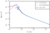 |
Fig. 1 Radial profile of the density in the (x–y)-plane at t≈2.5 kyr in the R–SINKt0 (purple line), R–NOSINKt0 (purple, dotted line), and PLUTO (blue line). At this stage, initial axisymmetry is maintained. Towards the center, the density settles in a plateau, forming a disk structure with an additional density bump in R–SINKt0 and PLUTO, while it continuously decreases in R–NOSINKt0 and forms a ring around 30 AU. |
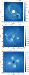 |
Fig. 2 Map of the density in logarithmic scale at the first fragmentation epoch (t≈4.5 kyr) in the disk plane in PLUTOx16 (top), R–SINKt0 (middle) and R–NOSINKt0 (bottom). PLUTOx16 and R–SINKt0 form a centrally condensed system whereas R–NOSINKt0 forms a multiple system. Forthe rest of the paper, we focus on a comparison between PLUTO and R–SINKt0. |
4 From cloud collapse to disk formation in a centrally condensed stellar system
In the following, we explore the early phases of massive star formation described in our numerical experiment, namely: first radial equilibrium reached, formation of a central accretion disk exhibiting a density bump, followed by the first fragmentation phase triggered by Toomre instability. At each step, we compare the outcomes of the RAMSES and the PLUTO runs, while focusing our in-depth analysis on the RAMSES simulations specific to the study presented in this paper.
4.1 Equilibrium and first fragmentation era
The cloud is initially gravitationally-unstable and leads to a global infall motion. The density in the central regions increases until it becomes optically-thick: it switches from isothermal to adiabatic. This is the first Larson core. As it contracts further, the gas temperature heats up and the thermal pressure increases accordingly. At the border of the Larson core, the gradient of thermal pressure becomes strong enough to halt the infalling material. Further over time, centrifugal acceleration increases due to infalling rotating material and finally dominates over thermal pressure gradients in setting a rotationally-supported structure: an accretion disk is born. Figure 3 shows the map of the radial velocity in the disk plane at ≈2 kyr in RAMSES (top) and in PLUTO (bottom). The accretion shock onto the disk is visible as the sharp transition between the red, infall region, and the white, disk region. RAMSES and PLUTO agree on the qualitative picture, namely, the onset of the adiabatic stage, formation of a Keplerian disk and formation of an accretion shock. They also agree on the size of the disk and its associated formation timescale.
After 2 kyr, a density bump forms between 30 and 50 AU in the RAMSES run, as shown on Fig. 1 and mentioned in Sect. 3. This structure will be studied in more details in Sect. 4.2. In a qualitative view, rotating infalling material appears to have “bounced” onto the central region. As mentioned in Sect. 3, a similar structure is present in PLUTO runs (see Fig. 1) but this structure is sharper in PLUTO as it is caused by several axisymmetrical accretion shocks propagating through the disk.
At this stage, within the innermost 30 AU, the total gas+sink mass is 0.37 M⊙ in RAMSES against 0.47 M⊙ at the same time in PLUTO. In RAMSES as in PLUTO, the bump is where the disk becomes (the most) Toomre-unstable and the first fragments form, breaking the axisymmetry, between t = 3 kyr and t = 4 kyr. The location of the bump, when fragmenting, is between 30 and 50 AU. The density map after fragmentation is displayed in Fig. 2. This is the first fragmentation epoch. We note that the number of fragments is different between the codes: 2 in PLUTO (one is being sheared in the view of Fig. 2), 3 in the RAMSES run. The initial perturbations are certainly introduced by numerical errors. Otherwise, m = 4 symmetry (following the Cartesian grid) in the RAMSES run and axisymmetry in the PLUTO runs should be perfectly conserved. It can be seen that fragments moved from their initial radius (i.e., the radius of the fragmenting structure). Indeed, they evolve on eccentric orbits, interacting with the central sink, with the background disk and with the other fragments. The disk size is similar in both codes. At this stage, due to different sink algorithms, the mass is naturally distributed in a different manner between the sink and the gas in the two codes: the sink mass is 1.14 M⊙ in RAMSES against 1.66 M⊙ in PLUTO. Zooming-out, the total gas+sink mass is 2.22 MQ within 100 AU and 2.57 M⊙ within 200 AU, in the RAMSES run. For comparison, the total gas+sink mass is 2.00 M⊙ within 100 AU and 2.56 M⊙ within 200 AU, in the PLUTO run, which give relative differences between codes of 11% and <1%, respectively.
To sum up, we followed the very early phases of massive protostellar collapse. RAMSES and PLUTO runs agree on the formation of a rotationally-supported structure (disk) and on the presence of an accretion shock at its border. A density bump is formed in both codes but for distinct reasons (see Sect. 4.2). It causes the first disk fragmentation phase as it is Toomre-unstable, at about the same time in RAMSES and PLUTO runs.
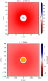 |
Fig. 3 Map of the cylindrical radial velocity at t≈2 kyr in the disk mid-plane in the RAMSES run (top panel) and in the PLUTOx16 run (bottom panel). The sink particle in RAMSES is represented by the white-filled, black circle; the sink cell in PLUTO is represented by the orange circle. Gas is dominated nearly everywhere by infall motions (red regions) until it shocks onto the flattened core, resulting in a radial velocity close to zero. |
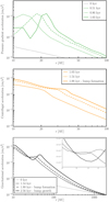 |
Fig. 4 Radial (cylindrical) acceleration due to thermal pressure gradient (top panel), centrifugal acceleration (middle panel), and gravitational acceleration (bottom panel) at distinct epochs to study the density bump formation, which is responsible for the first fragmentation. Only the radial gravitational acceleration is directed inward. In the zoom-in view of the bottom panel, it can be seen that the inward gravitational acceleration weakens around 30 AU at t≲2 kyr, so that gas accumulates into a bump. |
4.2 Density bump formation: an interplay between pressure gradient, centrifugal, and gravitational accelerations
We aim to understand how does the density bump form in the disk in RAMSES as it further triggers the first fragmentation phase. In order to do so, we compute the relevant accelerations at work in the cylindrical radial direction: centrifugal, thermal pressure gradient, and gravitational accelerations. Their radial profile is shown in Fig. 4 for the epochs of interest depending on the acceleration at play.
First, we find that the sum of the outward thermal pressure gradient and centrifugal accelerations balance the inward gravitational acceleration, ensuring equilibrium. This is linked to the pressure gradient stopping the gas at the border of the first hydrostatic core, indicated by the peak in the pressure gradient acceleration profile (top panel of Fig. 4). These forces are responsible for the accretion shock presented before. Finally, this structure (future disk) expands as the peak shifts towards a larger radius (see Fig. 3). It is flattened in the vertical direction due to rotation (e.g., Black & Bodenheimer 1976).
The infall of material brings additional specific angular momentum which eventually contributes to the centrifugal acceleration. Indeed, the initial rotation profile gives  . Angular momentum conservation for a portion of gas implies that its cylindrical velocity at a given final radius rf is υϕ,f = υϕ,i,rcyl,i/rcyl,f > υϕ,i (because of the infall motion). While the view exposed here neglects mixing, it is clear that υϕ increases locally due to the input of specific angular momentum associated with the infall. Since the centrifugal acceleration at a given cylindrical radius is proportional to
  and υϕ increases locally, as shown above, it increases very rapidly (see the bottom panel of Fig. 4) until it becomes the dominant force counter-balancing the gravitational acceleration: we refer to this equilibrium structure as a disk.
Initially, the gravitational acceleration increases in the central region as the mass increases. As the disk forms around the first Larson core, the mass distribution becomes highly anisotropic (while remaining axisymmetric) because of the centrifugal acceleration (Larson 1972). As a consequence of this new distribution, the gravitational acceleration decreases around 30 AU, as shown in the zoomed view in the middle panel of Fig. 4. Indeed, when mass accumulates at the border of the disk, it reduces the inward gravitational acceleration at smaller radius (see Appendix A of Tohline 1980). The anisotropy is crucial: in a spherically-symmetric density distribution, a gas portion located at a given radius only feels the gravitational acceleration due to the mass enclosed within this radius; the isotropic density distribution located further out does not contribute to the gravitational acceleration. In the same region, the centrifugal acceleration is not reduced because of angular momentum conservation: it can either stay constant, or increase because of additional input of infalling, rotating material with higher specific angular momentum. Then, the centrifugal acceleration starts to dominate over the gravitational acceleration locally. This is a runaway process: as the gas is given a positive radial velocity and is driven to larger radius, the gravitational acceleration is reduced even more, until an axisymmetric density bump forms. Two mechanisms moderate or stop this process. First, the accretion onto the sink removes material from the grid, which thus cannot participate to the bump growth. The second mechanism is the fragmentation of the disk. The disk is globally Toomre-unstable, but the location at which it is most unstable is in the density bump. The bump growth stops when the disk fragments, at the bump location, which occurs on an orbital timescale (Norman & Wilson 1978).
We address the robustness of the bump formation process (or its somewhat equivalent ring structure when no sink is present initially) in Appendix A.
4.3 Disk growth
Following the first fragmentation era and the formation of a dense halo (see Fig. 2), the central accretion disk grows as rotating gas falls in. As a diagnostic of the disk structure (and in particular, its outer radius), we compute the deviation from Keplerian frequency of the rotating gas around the central sink. We correct the Keplerian frequency by the sink “softening length” which softens the gravitational force (Bleuler & Teyssier 2014). Hence, the modified Keplerian angular frequency ΩK,soft is given by
 (6)
(6)
where rsoft is four times the finest spatial resolution here, Mgas(< r) is the mass enclosed in a radius r and Msink(r) is the sink mass for r ≥ rSOft and the fraction of the sink mass enclosed within a radius, r, for r < rsoft.
Figure 5 shows the deviation with respect to Keplerian frequency from 0 to 12 kyr, averaged over 4 kyr intervals, in the RAMSES and PLUTO runs. The gray area represents a ±10% deviation with respect to perfect Keplerian frequency. This figure shows a region of gas compatible with Keplerian rotation (i.e., in centrifugal equilibrium), already from the [0, 4] kyr time interval, in the RAMSES run. This is the accretion disk around the central star growing with time.
We notice that the deviation from Keplerian frequency in the RAMSES and PLUTO runs rarely deviate by more than 10% from the other, showing an overall correct agreement at following the disk formation epoch in terms of rotation support (deviation from Keplerian frequency) and disk size (transition from a mainly rotational support to infall motion). The disk build-up appears slightly more rapid in the PLUTO run, for any time interval. This suggests a faster collapse in PLUTO than in RAMSES. A possible explanation comes from the gas mass located outside the pre-stellar core in the RAMSES run, which may slightly slow down the collapse, in a similar manner as reported in Federrath et al. (2010). The higher resolution achieved in the central regions in PLUTO may also contribute to a faster collapse than in the RAMSES run.
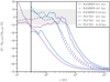 |
Fig. 5 Radial profile of the deviation from the Keplerian frequency. Purples curves refer to the RAMSES run and blue curves refer to the PLUTOx8 run. The Keplerian frequency is corrected by the sink softening length (Eq. (6)). For each radius, we compute the azimuthal median and average it in time (as indicated in the plot legend). The use of a median is meant to get rid of non-axisymmetries such as spiral arms (see OK20). The gray area points to a deviation of ±10% with respect to Keplerian frequency. The vertical line indicates the sink cell radius in PLUTO runs. Until t~12 kyr, disks are comparably Keplerian in RAMSES and PLUTOx8. |
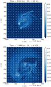 |
Fig. 6 Map of the density in logarithmic scale at t≈8 kyr (top panel) and t≈15 kyr (bottom panel) in the disk midplane in the RAMSES run. |
5 Disk dynamical state: evolution and fragmentation
In the following, we focus on the disk dynamical state and on the properties of its fragments, as those could collapse to form stellar companions. Part of the time evolution of the system in RAMSES is illustrated with density maps in Fig. 6. Hence, we start by looking at the stellar accretion history because its gravitational influence is decisive for the gas dynamics, which tends to settle in to a gravito-centrifugal equilibrium around the central star (Zinnecker & Yorke 2007) and for the disk stability as it sets the relative importance of the disk self-gravity (Kratter & Lodato 2016). This is also an opportunity to see how different subgrid methods for accretion compare together.
5.1 Mass accretion history of the central star
We start out by noting that the fragments formed following disk fragmentation in the RAMSES run, at about 4 kyr, are accreted eventually, similarly to the first fragments formed in PLUTO and shown in Fig. 2. Nevertheless, some of their initial orbits are stable until fragment-fragment interactions promote accretion. Those fragments contribute to the mass growth of the central sink particle or cell, which we detail below.
The sink mass in the RAMSES run and in the PLUTOx8 and PLUTOx16 runs is plotted as a function of time in the left panel of Fig. 7. As in the rest of the paper, the instant t = 0 kyr refers to the beginning of the simulation. We find that the overall evolution of the sink mass is qualitatively similar, with several accretion bursts during which the sink gains more than one solar mass. This is due to the accretion of fragments, whose formation is observed in both studies (Sect. 5.5). Meanwhile, the sink mass is always smaller in the RAMSES run as compared to PLUTOx16 and PLUTOx8, with a difference that can be as large as a factor of 2. Possible explanations for this quantitative discrepancy are the density threshold for sink accretion or the ability for the gas in our simulation to leave the sink volume while it directly enters the sink mass in PLUTO runs. To check the former, we run a similar simulation but with a density threshold ≈4 times smaller and the sink mass is nearly unchanged with 7.3 M⊙ at t≈13 kyr instead of 7 M⊙. This is consistent with Hennebelle et al. (2020), who report that the sink mass is marginally influenced by this threshold. To check the latter, we integrate the total inflow mass into a sphere of radius 30 AU centered on the sink. Since we do not output every iteration of the run, the inflow rate used to compute the total inflow mass is smoothed using a median over seven outputs (the time step between outputs is about 0.1 kyr). This total inflow mass, labeled Minflow,30AU, is displayed in the left panel of Fig. 7. The estimate Minflow,30AU compares well with PLUTOx8 and PLUTOx16, except for the period between ≈12 kyr and ≈15 kyr, in which run PLUTOx8 exhibits an accretion burst. Hence, the discrepancy between our sink mass and the PLUTO runs likely comes from the difference in the accretion model: a density threshold in RAMSES against a sink cell in PLUTO. In the former, gas is allowed to leave the sink volume without being accreted and the sink actually plays the role of boundary conditions for the disk (Hennebelle et al. 2020), while it is directly attributed to the sink mass in the latter and associated with boundary conditions on the hydrodynamical variables.
The accretion rate is displayed (in logarithmic scale) as a function of time in the right panel of Fig. 7. It oscillates between a low accretion state with  and a high accretion rate state with values higher than
  . The accretion rate in the low state is similar to that found in PLUTOx16. The high state gives a smaller accretion rate than what is reported by OK20. However, this state corresponds to the epochs when fragments are accreted and fragments have typically the same mass in both studies (see Sect. 5.5), so the quantitative difference partially comes from the different time bin (larger in our study) to compute the instantaneous accretion rate. Both studies exhibit a similar number of accretion bursts.
 |
Fig. 7 Sink mass as a function of time in the RAMSES run against the PLUTOx8 and PLUTOx16 runs (left). The quantity Minflow 30 AU is the total mass flowing into a central sphere of radius 30 AU, reproducing the accretion model of PLUTO runs. Accretion rate onto the sink as a function of time in the RAMSES run against the PLUTOx16 run (right). |
5.2 Disk Keplerían motion
Figure 8 shows the radial profiles of the deviation from Keplerian frequency, defined using Eq. (6) and the density in the RAMSES and PLUTO runs. It can be seen in the left panel of Fig. 8 that the gas is slightly sub-Keplerian between 30 AU and a few hundreds of AU, especially between 16 kyr and 20 kyr (down to ≈–20%). On the opposite, the same region in PLUTOx8 shows a deviation between –10% and 10%. If the gas Keplerian motion should be used as a proxy for the disk radius, then the drop in deviation from Keplerian frequency points to a disk radius of ≈550 AU for the interval [12, 16] kyr and either ≈70 AU (using the first drop) or ≈750 AU (using the second drop) for the interval [16, 20] kyr, against ≈900 AU for the interval [12, 16] kyr and ≈ 1000 AU for the interval [16, 17.5] kyr in PLUTOx8. Furthermore, we computed the thermal pressure gradient acceleration and we note that it is one order of magnitude too small to compensate this sub-Keplerian motion and ensure equilibrium. Thus, the disklike structure we obtain is not at equilibrium. We observe that the sub-Keplerian region coincides with the region where the gas dynamics is dominated by interactions between fragments (collisions, gravitational interactions) and with the central star. For instance, at ~18 kyr, a clump (not hot enough to be detected as a fragment, see Sect. 5.5) is partially disrupted in the vicinity of the central star. Part of the debris stream is projected with radial velocities of the order of l0 km s−1. The stream collides with the infalling, rotating gas, so the region swept by the stream only contains slowly-rotating, sub-Keplerian gas. Moreover, we find that the north-south symmetry has been broken, which we attribute to the multiple fragment collisions.
As shown in the right panel of Fig. 8, the density in the central region is roughly in agreement with the findings of PLUTOx8. We recall that we took the azimuthal median for each radius, hence, the dense fragments and other non-axisymetries have been smoothed. This is true as long as more than 50% of the cells within those bins are in a common state, referred to as the background disk state in OK2O. The drop in density around 1000 AU, which could be used to define the primary disk as well, is found at a similar radius in both studies after 16 kyr and with a slightly smaller radius in PLUTOx8 for [12, 16] kyr. A first drop in density is also present at ≈70 AU for the [16, 20] kyr interval, at the same position as the drop in the deviation from Keplerian frequency previously reported. This indicates the low density region produced by tidal disruptions of fragments.
As a side note, the spikes visible in the deviation from Keplerian frequency and in the density profiles at about 3000 AU correspond to a fragment that has been ejected by fragment-fragment interactions around 7 kyr. It appears to be gently falling back onto the central region.
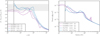 |
Fig. 8 Radial proflies of the deviation from Keplerian frequency (left panel) and the density (right panel) in the RAMSES run and in PLUTOx8. For each radius, we compute the azimuthal median and average it in time (as indicated in the plot legend). The vertical line indicates the sink cell radius in PLUTO runs. |
5.3 Impact of numerical methods on the Keplerian motion
5.3.1 Grid (de-)refinement
In the following, we address the possible impact of numerical methods on the sub-Keplerian disk profile. To understand whether the AMR refinement and de-refinement could artificially prevent the disk from relaxing to quiescence, we run a similar simulation from the start but with a partially-fixed grid. We use a geometrical criterion to fix the spatial resolution to 2.5 AU up to ≈200 AU from the central star and to 5 AU up to 400 AU, in the disk plane and within a disk thickness of 30 AU. This results in a number of cells of size 2.5 AU in a cylinder of radius 200 AU and height 30 AU centered onto the sink multiplied by ~4 (from about 60 000 cells to 240 000 cells). Further away, between radii of 200 AU and 400 AU, the number of cells of size 5 AU is multiplied by ~6 (from about 15 000 cells to 90 000 cells). Additional refinement based on the standard Jeans length criterion is allowed. We obtain similar results in terms of Keplerian motion as in run RAMSES. Hence, the sub-Keplerian motion is not due to the AMR grid.
5.3.2 Axisymmetric gravitational potential on a Cartesian grid
We also check whether this could come from a bad sampling of the density on a Cartesian grid, which should, in the case of an accretion disk, take a nearly axisymmetric distribution. First, we obtain a nearly Keplerian disk until t≈12 kyr and therefore the loss of Keplerian motion is unlikely to be caused by the grid being Cartesian. For safety, we can check how is sampled a spherically-symmetric potential by computing the gravitational potential of the pre-stellar core at t = 0 (the bad sampling would be linked to the Cartesian grid and therefore should be already visible at t = 0), and compare it to the analytical, textbook value. We obtain an error of 2%. This suggests that the sub-Keplerian frequency, which reaches –20% is not a consequence of a bad sampling of the density distribution by the Cartesian grid. This is consistent with the study of Lyra et al. (2008), who ran simulations of disks in a Cartesian grid and were able to reproduce standard features (such as equilibrium) obtained in cylindrical and spherical codes (see also the code comparison by De Val-Borro et al. 2006). Hence, the origin of the discrepancy between RAMSES and PLUTO is not attributable to the grid.
5.3.3 Importance of the fragments dynamics and sink mass
Finally, to assess the dynamical origin of both the sub-Keplerian motion and the north-south asymmetry, we perform an identical simulation with a finest resolution of 10 AU (see Appendix B). Indeed, this resolution should slightly under-resolve the dense structures, and therefore reduce the impact of collisions. Moreover, it shifts the central sink accretion radius from 10 AU to 40 AU, so there is less gravitational energy available to fuel the tidal disruptions. In this run (plot not shown here for conciseness), we find the vertical structure to remain roughly symmetric up to 20 kyr. Furthermore, the rotation profile is closer to Keplerian rotation, with a smallest value of –15% to –20% (see Fig. B.3). Meanwhile, the sink mass evolution is similar, at late times, to that presented in Fig. 7 for run RAMSES (see Fig. B.2). Hence, we conclude that the sub-Keplerian motion and north-south asymmetry are partially linked to the dynamics, that is, collisions and tidal disruptions in the disk-like structure.
Moreover, the total mass of the fragments during the interval [16, 20] kyr is around 6 M⊙ on average in RAMSES (more details in Sect. 5.5), while the central star mass is between 11 M⊙ and 16 M⊙. In run PLUTOx8, the star mass is 17 M⊙ at t = 16 kyr and the maximal mass of a fragment is between 3 M⊙ and 5 M⊙. Here, the central star dominates only marginally and locally, the total gravitational potential. Beyond a few hundred AU, the disk self-gravity dominates, thus it is more prone to gravitational instabilities (e.g., Kratter & Lodato 2016) and less likely to reach quiescence. Hence, the accretion model impacts the sink mass, as shown in Sect. 5.1 and it is certainly responsible for the discrepancy regarding the disk equilibrium (i.e., Keplerian motion; indeed, thermal support is much smaller than rotation support).
5.3.4 Discussion on the Keplerian motion
Overall, we find that the RAMSES run exhibits a more dynamical or chaotical, disk-like structure than in OK20, where the disk is Keplerian and therefore at equilibrium between centrifugal and gravitational accelerations. No quiescence state is reached by the end of the simulated time (≈20 kyr) unlike the PLUTO runs. This sets into question whether the gas orbiting the sink in the RAMSES run should be labeled a (sub-Keplerian) disk and whether it would relax to a Keplerian disk state at later times, once the central mass becomes sufficiently massive. A possibility to explain the discrepancy between OK20 and the present result lies in the mass growth of the central star and the fragments, because the disk stability increases with the star-to-disk mass ratio (Kratter & Lodato 2016). Indeed, we found a smaller stellar mass and slightly more massive fragments than OK20, resulting in a less stable disk than in their study. The accretion model, namely a sink cell with inflow boundary condition in OK20, and a density threshold in the sink volume in our case, is likely responsible for this discrepancy in the sink mass. In any case, it suggests a larger impact from the accretion model and the modeling of the central 30 AU in radius than from grid effects (AMR and Cartesian). Nevertheless, differences in the propagation of spiral waves, which contribute to angular momentum redistribution and subsequent accretion, on a spherical grid and on a Cartesian grid could also be at work to explain part of the aforementioned discrepancies. Running the same simulations with a SPH code would allow for a complementary point of view. We leave such comparison studies to a future work.
5.4 Fragments tracking
In the following, we describe our study of the temporal evolution of the fragments. First, we implemented the procedure presented in OK20 in order to detect fragments in RAMSES outputs and identify them from one output to the next one. In a nutshell, for a given output, n, we extracted the temperature map in the (x = 0, y, z)-plane and we convolved it by a Gaussian filter to smooth the non-axisymmetries induced by spiral arms. Then, we computed the azimuthal median profile of the temperature and, in each cell, we retrieved the corresponding value to identify hot spots (i.e., zones of higher temperature than their corresponding azimuthal median). A temperature threshold of 400 K was then used to select the position of the remaining hot spots. The size of hot spots is set to 40 AU in radius, as in OK20. With our finest resolution of 2.5 AU and a refinement criterion based on the Jeans length, this ensures that the diameter of a fragment is sampled by 16 cells. Once the position is obtained, we collect the data (central temperature, mass, density, and velocity vector) of each fragment. We used the output n + 1 to extract the positions of new hot spots and computed the expected position of the old hot spots using a linear expansion in time, that is, rexp = rn + υr,n(tn+1 – tn) and ϕexp = ϕn + υϕ,n/rn(tn+1 – tn), for the radius and azimuthal angle ϕ, respectively, where the subscript “exp” stands for “expected” and n for the output number. Comparing the positions of new hot spots with the surroundings of the expected position of old hot spots, we determine whether or not they correspond to the same physical fragment. Finally, we manually checked the continuity of the orbits.
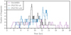 |
Fig. 9 Number of fragments as a function of time. Only fragments with a lifetime longer than 200 yr are shown. |
5.5 Fragments properties
Fragments form within spiral arms or following spiral arm collisions, in RAMSES as in PLUTO, as already reported in several studies (see e.g., Bonnell 1994; Bonnell & Bate 1994a). They orbit around the central star on eccentric orbits and eventually get destroyed by various processes: tidal disruption after approaching the central star (e.g., fragments #1 and #8), thermal expansion (e.g., fragment #13), or shear when transported over a spiral arm (e.g., fragment #14). These processes occur in both RAMSES and PLUTO runs.
First of all, the number of fragments is in correct agreement between RAMSES (and among the RAMSES runs, see the convergence study in Appendix B) and PLUTO. Figure 9 shows the number of fragments detected as a function of time. The number of fragments is on the same order of magnitude and varies between 0 and 2 in RAMSES and 0 and 4 in PLUTO. The few times when the number of fragments is very distinct in RAMSES and PLUTO are associated with a transient peak of fragment formation or destruction, for instance, at ≈9 kyr, run PLUTOx8. Such a peak (as also visible at ≈12 kyr in PLUTOx16) shows how nonlinear the formation and destruction of fragments can be, as new collisions between fragments and spiral arms can occur and either trigger new fragment formation or lead to their destruction or mergers, thereby reducing their number. Hence, rather than focusing our study on the exact fragment number at a given time, we are interested in statistical trends and, more importantly, on the physical origin of those trends. We note that the total fragment mass (see below) does not follow the peak behaviour reported above, suggesting that it is associated with low-mass fragments whose feedback on the background disk properties is small; hence, we treat this event as transient and not decisive for the rest of the simulation. Interestingly, a fragmentless disk, which is product of simultaneous fragment-destruction events, is reported in PLUTOx8 at 11–12 kyr and in RAMSES at 10–11 kyr. A plausible outcome of such a fragmentless period would be for the primary disk to enter a quiescent phase as a result of the reduced activity in the disk, and provided that the central star is massive enough to stabilize it. This is not the case in RAMSES but is the case at late times in PLUTOx8, when the temperature increase due to stellar irradiation in the innermost parts of the disk also contributes to the stabilization. Overall, except for transient events of fragment formation or destruction, RAMSES and PLUTO yield very consistent results with respect to the number of fragments present on the disk as a function of time.
We now turn to the mass of fragments. Figure 10 shows the total (top panel) and individual (bottom panel) mass of the fragments as a function of time. The total fragment mass smoothly increases with time and is, on average, ~2–2.5 M⊙ in both codes. Up to ~ 10 kyr, the total fragment mass evolution is very similar in all runs. This is understandable as the mass budget for fragments is linked to the growth of the primary disk. After 10 kyr, the total fragment mass abruptly decreases in RAMSES (except for a finest resolution of 10 AU, see Appendix B.2) and PLUTOx8 as an event of simultaneous fragment destruction occurs, as previously reported. Individually, the fragment masses range from a fraction of a solar mass up to six solar masses. In comparison, the most massive fragment is 5 Mθ in run PLUTOx8 and 3M⊙ in run PLUTOx16, as indicated by the dashed lines. The high mass reached by fragments #11 and #14, between 3 M⊙ and 6 M⊙, suggests that they had the potential to form rapidly a massive companion. Moreover, we notice a trend for forming more massive fragments at later times than early times, in agreement with OK20. Indeed, the initial mass enclosed within a radius r increases with the radius as r1.5, so there is more gas available then. Another possibility would be the build-up of the accretion structure around the primary sink, but as discussed above (Sect. 5.2), such a structure is not at equilibrium in the RAMSES run – in contrast to what was found in OK20.
Let us now focus on the fragment temperature. Figure 11 shows the temperature of the fragments as a function of time. The gray band indicates the H2 dissociation limit T ~ 2000 K, as in OK20. Fragments reaching this limit are expected to undergo second collapse and form second Larson cores (see e.g., Vaytet et al. 2013 and Bhandare et al. 2020 for a dedicated study on the second core formation). We report that nine fragments reached this limit, against ten in run PLUTOx16 and four in run PLUTOx8. Except for fragment #11, whose temperature is due to a collision event that compresses the gas adiabatically because it is optically thick – up to ρ≈5 × 10⁻⁹g cm−3, the fragments’ temperature is in a range that is still consistent with the PLUTO runs. The fragment temperature appears correlated with the fragment density (see Fig. 10, the radius being fixed) suggesting adiabatic heating for all fragments.
Figure 12 shows the distance to the primary sink when fragments are detected, as a function of time. As the disk grows, fragments can form at larger distances from the star. Nevertheless, the formation of fragments at smaller radii is not suppressed (see e.g., fragments #11 and #14). Fragments #6 and #7 form from the collision of two flows and migrate outwards while reaching the temperature threshold for detection, which explains the large distance at which they form. Except for those two fragments, the distance is consistent with the maximal distance of newly born fragments in the PLUTOx8 run, plotted as the black curve.
Overall, the fragments properties are in agreement between the RAMSES and the PLUTO runs. This indicates that despite distinct radiation-hydrodynamical approaches, both codes reach a satisfying agreement at modeling the local thermodynamical behaviour of gaseous fragments in a massive protostellar disk.
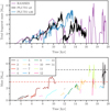 |
Fig. 10 Total mass in all runs (top) and individual mass in RAMSES (bottom) of the fragments as a function of time. Only fragments with a lifetime longer than 200 yr are shown. For visibility and comparison, in the bottom panel, the black and red dashed lines show the highest fragment mass in run PLUTOx8 and PLUTOx16, respectively. |
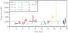 |
Fig. 11 Central temperature of the fragments as a function of time. Only fragments with a lifetime longer than 200 yr are shown. |
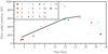 |
Fig. 12 Distance of newly born fragments to the central star, as a function of time. Only fragments with a lifetime longer than 200 yr are shown. The black curve indicates the maximal distance of newly born fragments in the PLUTOx8 run. |
6 Conclusions
We present self-gravity radiation-hydrodynamical simulations of the collapse of a massive pre-stellar core performed with the Cartesian AMR code RAMSES and we carry out a comparison with the highest resolutions runs of Oliva & Kuiper (2020), performed with a modified version of the code PLUTO using a grid in spherical coordinates.
As a preliminary step, we chose the RAMSES numerical setup for comparison to PLUTO. We compared two RAMSES runs, one with a unique, central, fixed sink particle and the other without any initial sink, but including the possibility to form sinks later on. Those two runs lead to qualitatively distinct systems: the former leads to a centrally-condensed system, while the latter ends up in a multiple stellar system born out of Toomre instability seeded by the Cartesian grid. As the divergence is inherited from the first fragmentation phase, it shows how crucial is fragmentation in the innermost regions of the cloud for the future evolution of the system. In this problem, the numerical caveats introduced by the use of sink particles and by the grid. It is not yet clear which of the two is the most realistic one. For future studies, the issue of the instability seeded by the grid could be overcome by introducing additional dominant perturbations (see e.g., Boss & Bodenheimer 1979; Commerçon et al. 2008) or by accounting for the inflow from larger scales (e.g., Vázquez-Semadeni et al. 2016; Padoan et al. 2020) while still resolving disk scales (Lebreuilly et al. 2021). Additionally, turbulence in the massive pre-stellar core could be included to match the observational constraints of some pre-stellar cores (e.g., Beuther et al. 2007; Bontemps et al. 2010; Palau et al. 2013; Girart et al. 2013; Fontani et al. 2016; Nony et al. 2018) and may introduce density and velocity perturbations dominating over numerical ones.
To perform the code comparison in the context of a centrally-condensed system, we chose the RAMSES run with a unique, central, initial sink particle, as it compares qualitatively with the runs presented in Oliva & Kuiper (2020). In the early phases of the collapse, gas free-falls towards the central region. The central density increases and switches from isothermality to adi-abaticity. Additional infall of rotating gas triggers the formation a rotationally-supported disk whose border is the location of an accretion shock. A good agreement between RAMSES and PLUTO is reached regarding the timeline of these events, as well as on the core and disk radius. A “rotational bounce” occurs in the RAMSES run and forms a density bump, while the PLUTO runs show the formation of axisymmetric shocks on the same timescales and propagating through the disk. This discrepancy might be due to the fine treatment of self-gravity, pressure gradient and centrifugal acceleration while conserving linear and angular momentum in a tiny (<50 AU in radius) portion of the (20 000 AU in radius) cloud. In RAMSES the disk fragments at the location of the bump, which is Toomre-unstable, and in PLUTO the early disk evolves two spiral arms which fragment due to their high density (low Toomre-parameter value). These events occur on similar timescales: this is the first fragmentation era. The accretion disk progressively grows around the central star. It is consistent with Keplerian rotation in both codes, from its formation epoch to 12 kyr. Using the Keplerian frequency as a criterion to define the disk size, both codes show a good agreement: a difference of a few percent.
The accretion disk grows with time and the star gains mass, while fragments form continuously in the disk. We detected and followed those fragments forming around the central star via their temperature. The number of fragments reaching the H2 dissociation limit and their overall temperature is in agreement between the two codes, as well as their formation position. Some of them are slightly more massive in the RAMSES runs than the fragments formed in the PLUTO runs (6 against 5 M⊙ for the most massive fragments formed in each code), but the two codes find an overall satisfying agreement on the fragment properties. This indicates that, in the present radiation-hydrodynamical frame with self-gravity, the local thermodynamics of fragments is consistent between RAMSES and PLUTO.
In the disk dynamical epoch, covering its growth and fragmentation, the disk is found to be sub-Keplerian over hundreds of AU in RAMSES, while it is Keplerian in PLUTO. We tested several hypotheses to explain this result: the outcome of numerical methods (grid refinement and de-refinement, bad sampling of the nearly axisymmetric gravitational potential on a Cartesian grid) and the relevance of fragments dynamics and of the sink mass. We found that the disk sub-Keplerian motion originates from tidal disruption of fragments and collisions, which strongly modify the velocity field in the disk region. It produces spiral arms sweeping off the gas, slowing down the infall and reducing the amount of rotating gas around the central star. Furthermore, the dynamics of fragments has more impact in a system where the disk-(and fragments)-to-star mass ratio is high. In fact, this ratio is higher in RAMSES than in PLUTO. Indeed, while fragments are slighlty more massive in RAMSES, the stellar mass is about twice smaller as compared to PLUTO. We hypothesize that this discrepancy originates from the stellar accretion model. Indeed, in RAMSES, the sink only accretes gas above a given, user-defined (in the simulations presented here), density threshold. There is an additional constraint of not accreting more than 10% of the amount of gas above this threshold at each time step. Meanwhile, the accretion procedure in PLUTO represents a 100% efficiency with no density threshold: the gas entering the sink cell is accreted. When mimicking the accretion model of PLUTO (i.e., all the gas entering the sink volume is accreted) in the RAMSES outputs, we reproduce quite successfully the accretion history of the PLUTO runs. Apart from this discrepancy, we mention nevertheless that the accretion history is qualitatively similar in RAMSES and PLUTO and consists both of continuous accretion and accretion bursts associated with fragments being accreted. The order of magnitude of the stellar mass and of the accretion rate is similar in both codes. However, as we show, a factor of two on the stellar mass is crucial for the dynamics of the massive protostellar disk at such early stages of the protostellar evolution phase. This suggests that the details of accretion mechanisms, based on star-disk interaction, are not only important for the stellar growth but also for the disk equilibrium and for the properties of the ensuing multiple stellar system.
We conclude that the differences in the initial fragmentation phase, potentially triggered by numerical choices (the grid, the use of sink particles, etc.), have more of an impact on the final multiplicity of the system than the choice of the code itself between RAMSES and PLUTO, when smooth initial conditions are employed.
Acknowledgments
Acknowledgements.
R.M.R. thanks the referee for helping improving this manuscript. R.M.R. thanks Peggy Varniere and Ugo Lebreuilly for fruitful discussions. R.M.R. acknowledges Patrick Hennebelle for his insights on numerical angular momentum conservation. This work was supported by the CNRS “Programme National de Physique Stellaire” (PNPS). This work has received funding from the French Agence Nationale de la Recherche (ANR) through the project COSMHIC (ANR-20-CE31-0009). The numerical simulations we have presented in this paper were produced on the CEA machine Alfvén and using HPC resources from GENCI-CINES (Grant A0080407247). The visualisation of RAMSES data has been done with the OSYRIS python package, for which RMR warmly thanks Neil Vaytet. G.A.O.-M. acknowledges financial support by the Deutscher Akademischer Austauschdienst (DAAD), under the program Research Grants – Doctoral Programmes in Germany, and financial support from the University of Costa Rica for the obtention of his doctoral degree. R.K. acknowledges financial support via the Emmy Noether and Heisenberg Research Grants funded by the German Research Foundation (DFG) under grant nos. KU 2849/3 and 2849/9.
Appendix A Density bump or ring formation
Appendix A.1 Dependence on numerical and physical parameters
In the following, we describe how we performed several checks to assess the robustness of the density bump or ring structure reported in the main text with respect to thermodynamics, as well as the physical and numerical parameters. As shown in Sect. 3, removing the sink particle in order to deal with self-gravity hydrodynamics only gives a ring instead of a density bump. The ring interior is made of low-density, sub-Keplerian material, but the processes of density bump and ring formation are similar. Hence, we further focus on how the ring forms because it removes any influence from the central sink.
In the absence of a sink particle, to check whether the ring formation is a purely dynamical effect or if it is linked to the thermodynamics, we turned off the FLD module and switched to a barotropic equation of state, using the density threshold for adiabaticity as 10−13g cm−3, as in Cha & Whitworth (2003), we find that the outcome is unchanged. Finally, we switched to an isothermal equation of state: the rebound occurs on the most central and densest region because of the pressure gradient (as in Larson 1972; Black & Bodenheimer 1976). This time, the pressure gradient has been built only by the density and not by the temperature (as in the barotropic and FLD cases, where pressure increases along with the temperature). This confirms the initial dynamical role of pressure gradient in forming this protostellar ring. We mention that, due to the aforementioned importance of pressure gradient forces, the label “rotational bounce” has been challenged by Narita et al. (1984).
In addition, we ran other simulations to explore the role of numerical and physical parameters on ring formation. We find this ring to be a robust feature with respect to the Riemann solver (Lax-Friedrich and HLLD, Miyoshi & Kusano 2005, which is less diffusive) to the initial rotation profile in the inner 30 AU (no rotation, solid-body rotation, and differential rotation), to the initial density profile in the inner 30 AU (plateau or power-law), and to the numerical resolution (from 10 AU to ≃0.3 AU resolution), making the angular momentum diffusion origin less plausible. Changes performed within the inner 30 AU were motivated by this size corresponding to the sink cell in OK20, adding several degrees of freedom in our simulations. Finally, it is certainly dependent on (other) initial conditions, as we did not report it in Mignon-Risse et al. (2020) nor Mignon-Risse et al. (2021b).
Appendix A.2 Code comparison
A density bump was present in PLUTO runs (Fig. 1), formed from accretion shocks and rapidly fragmented into two pieces (Fig. 2). Hence, the origin of the structure is likely to be different from the explanation above. Indeed, rotation only plays a role in the bump formation in PLUTO by flattening the density towards the mid-plane, the first hydrostatic core is initially located within the sink cell, the density (contributing to the pressure gradient) is affected by the inner, zero-gradient, and boundary condition; thus the gas cannot exit the sink cell to feed the structure, unlike the case of our simulation. In a Cartesian AMR simulation such as the RAMSES run, the most central region suffers from the low angular resolution of the orbital elements. Indeed, the region concerned with the ring is very small compared to the size of the system: its formation and evolution are certainly strongly affected by minor errors in angular momentum conservation (Larson 1972; Tscharnuter 1975; Tohline 1980; Gingold & Monaghan 1983). More in-depth works are required here.
The ring formation we report here is, however, reminiscent of early analytical works (Tohline 1980), numerical studies with SPH codes (e.g., Bonnell & Bate 1994b; Cha & Whitworth 2003; Hennebelle et al. 2004), 2D axisymmetric calculations (Narita et al. 1984), and nested grids (Matsumoto & Hanawa 2003); we also refer to the review by Larson (2003) and the comparison study performed by Bodenheimer & Tscharnuter (1979). Further studies on such ring formation are needed, as the ring (or density bump in presence of a central sink particle) is very unstable and can naturally lead to multiple system formation (Norman & Wilson 1978). Any other angular momentum transport mechanism than those included in this study could also prevent ring formation in astrophysical systems.
Appendix B Convergence study in RAMSES
We considered three runs with a finest AMR level of 13 (Low–res run), 14 (Mid–res run), and 15 (High–res run) to perform a convergence study. The High–res run corresponds to the fiducial RAMSES run presented in the main text. The aforementioned AMR levels result in physical finest resolutions of 10 AU, 5 AU, and 2.5 AU, respectively.
Appendix B.1 Disk rotation support and stellar mass growth
The deviation from Keplerian frequency during the disk formation and growth phase is shown in Figure B.1. At small radii, the same trend is visible in almost all runs and epochs with a decreasing deviation from Keplerian frequency as r goes to zero (super-Keplerian frequency at small radius is always transient). This effect is simply shifted to larger radii at lower resolution because the sink accretion radius is multiplied by two as the refinement is reduced by one level. There is an overall agreement on the disk Keplerian motion. We note the presence of a sub-Keplerian region around 200 AU in the Mid–res run in the 8–12 kyr epoch.
The mass history of the central object is shown in Fig. B.2. The final stellar mass is consistent from one run to the other with a deviation of about 15%. However, a comparison at a given time is made difficult by major accretion bursts, for instance, in the Mid–res run at 11 kyr. This event is connected to the non-Keplerian region reported above in the [8, 12] kyr epoch, showing once again the importance of the dynamics of fragments for the computation of the Keplerian frequency. Noticeably, the stellar mass growth in the Low–res run is delayed compared to the other runs. In fact, the first core density does not reach the accretion threshold before the ring starts forming and expelling gas from the center, thus starving the sink for a few kyr until the ring fragments. However, the fragments originating from the ring are eventually accreted by the star so it finally catches up with the High–res run accretion history.
The deviation from Keplerian frequency during the disk dynamical epoch is shown in Figure B.3. Qualitatively, runs Low–res and High–res exhibit at least once the presence of non-Keplerian regions in what would be expected to be the disk region. This occurred before for run Mid–res, between 8 and 12 kyr, when a major accretion burst occurred while the sink mass was still rather small (5M⊙). There is nevertheless a good agreement between the Mid–res and High–res runs for the disk radius in the [12, 20] kyr interval. The disk radius is larger in the Low–res run, while until the [8, 12] kyr epoch it was consistent with the Mid–res and High–res runs. As already underlined in the main text, this is attributable to the dynamics of fragments. At lower resolution, there is less gravitational energy to tap in during a close encounter with the central sink since it cannot get as close to the sink as in higher resolution runs. Hence, there is less kinetic energy for the fragments to destabilize the disk Keplerian motion. The regions that are non-Keplerian, from 400 to ≳ 1000 AU in run Low–res, indeed coincide with the region in which the two densest disk fragments are located, but their drops in Keplerian frequency are shallower than in the Mid–res and High–res runs. Moreover, a fragment’s disruption does not just affect the Keplerian motion at a given time. When it occurs, the post-disruption region is not centrifugally-supported so the infalling gas from larger scale penetrates this region until it reaches the centrifugally-supported disk and contributes to its build-up there. Applying this reasoning to the High–res run, part of the infalling material at epoch [16, 20] kyr eventually contributes to bringing the [100 – 400] AU region back to Keplerian motion instead of increasing the radius of the global disk-like structure. This explains why the disk is larger in run Low–res.
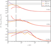 |
Fig. B.1 Radial proflies of the deviation from Keplerian frequency for various resolutions in the disk formation epoch, covering (from top to bottom) the [0, 4] kyr, [4, 8] kyr, and [8, 12] kyr time intervals. The vertical line indicates the sink particle accretion radius in the AMR513 run. |
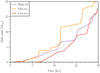 |
Fig. B.2 Sink mass as a function of time for various resolutions. |
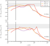 |
Fig. B.3 Radial profiles of the deviation from Keplerian frequency for various resolutions in the disk dynamical epoch, covering (from top to bottom) the [12, 16] kyr and [16, 20] kyr time intervals. The vertical line indicates the sink particle accretion radius in the AMR513 run. |
Appendix B.2 Fragments properties
From top to bottom, Fig. B.4 shows the number of fragments, total fragment mass, fragment temperature, radius of formation in runs Low–res (red), Mid–res (orange), and High–res (violet). The number of fragments is between 0 and 3 in run High–res, between 0 and 4 in run Mid–res and between 0 and 3 in run Low–res, showing a good overall agreement. The total fragment mass shows the same increase trend in runs Mid–res and High–res (also reported in the main text, in PLUTO runs), with a similar drop between 10 and 11 kyr, which is not the case in run Low–res, suggesting again that there is not enough gravitational energy to tap in during an accretion event to prevent further disk fragmentation. The fragment temperature is slightly smaller in run Mid–res than in High–res – and even smaller in run Low–res, in agreement with the adiabatic contraction heating mechanism. However, fragments formed in Mid–res can still reach the H2 dissociation limit temperature and exhibit a temperature spike, as in run High–res, while it is not the case in run Low–res; this suggests that the 10 AU resolution in Low–res is insufficient, for this particular setup – in comparison with the behaviour observed in runs Mid–res and High–res. As shown on the bottom panel of Fig. B.4, the radius at which fragments form can increase with time, as the disk size increases (as shown in the main paper), although fragments can still form as well in the innermost parts of the disk. The new fragments detected at more than 1000 AU in run Low–res come from the close interaction between two fragments and their spiral arms, which periodically collide, then fade away and collide again, thus producing a nearly periodic change in the number of fragments between 14 kyr and 17 kyr and similar radii of new fragment formation.
The fragment properties are qualitatively consistent between runs Mid–res and High–res, although the number of fragments is slightly higher in run Mid–res, suggesting that a resolution of 5 AU is sufficient to get a consistent qualitative picture (no convergence can be fully achieved since other mechanisms will eventually take place on smaller scales, be it disk turbulence or star-disk interactions) in this particular setup.
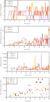 |
Fig. B.4 Number of fragments, total fragment mass, fragment temperature, and radius of formation for various resolutions, shown from top to bottom. Only fragments with a lifetime longer than 200 yr are shown. |
Appendix C Computational cost and carbon footprint estimate
Table C.1 gives the computational cost of the simulation presented in the main text and of the lower-resolution simulations presented in Appendix B. The total is a lower limit since others runs have been performed to test various hypotheses (see e.g., Sect. 5.2). As the AMR grid refines regions of interest, in particular around stellar companions, the cost does not strictly scale with the resolution, as could be expected. Simulations have been performed over 64 CPU cores. We note that the CO2,e (CO2 equivalent) carbon footprint has been computed using the estimate of 4.68 g/hCPU (Berthoud et al. 2020).
Computational cost (in CPUkhr) and CO2,e footprint estimate (in kg) of the simulations presented in Sect. B.
References
- Adams, F. C., Ruden, S. P., & Shu, F. H. 1989, ApJ, 347, 959 [Google Scholar]
- Ahmadi, A., Kuiper, R., & Beuther, H. 2019, A&A, 632, A50 [NASA ADS] [CrossRef] [EDP Sciences] [Google Scholar]
- Bate, M. R. 2009, MNRAS, 392, 590 [Google Scholar]
- Bate, M. R., Bonnell, I. A., & Price, N. M. 1995, MNRAS, 277, 362 [Google Scholar]
- Bate, M. R., Bonnell, I. A., & Bromm, V. 2002, MNRAS, 336, 705 [Google Scholar]
- Berthoud, F., Bzeznik, B., Gibelin, N., et al. 2020, Estimation de l’empreinte carbone d’une heure.coeur de calcul [Rapport de recherche] UGA - Université Grenoble Alpes - CNRS - INP Grenoble - INRIA, ffhal-02549565v5f [Google Scholar]
- Beuther, H., Churchwell, E. B., McKee, C. F., & Tan, J. C. 2007, Protostars and Planets V, eds. B. Reipurth, D. Jewitt, & K. Keil (Tucson: University of Arizona Press), 165 [Google Scholar]
- Beuther, H., Mottram, J. C., Ahmadi, A., et al. 2018, A&A, 617, A100 [NASA ADS] [CrossRef] [EDP Sciences] [Google Scholar]
- Beuther, H., Ahmadi, A., Mottram, J. C., et al. 2019, A&A, 621, A122 [NASA ADS] [CrossRef] [EDP Sciences] [Google Scholar]
- Bhandare, A., Kuiper, R., Henning, T., et al. 2018, A&A, 618, A95 [NASA ADS] [CrossRef] [EDP Sciences] [Google Scholar]
- Bhandare, A., Kuiper, R., Henning, T., et al. 2020, A&A, 638, A86 [NASA ADS] [CrossRef] [EDP Sciences] [Google Scholar]
- Black, D. C., & Bodenheimer, P. 1976, ApJ, 206, 138 [NASA ADS] [CrossRef] [Google Scholar]
- Bleuler, A., & Teyssier, R. 2014, MNRAS, 445, 4015 [Google Scholar]
- Bodenheimer, P., & Boss, A. P. 1981, MNRAS, 197, 477 [CrossRef] [Google Scholar]
- Bodenheimer, P., & Tscharnuter, W. 1979, A&A, 74, 288 [NASA ADS] [Google Scholar]
- Bonnell, I. A. 1994, MNRAS, 269, 837 [CrossRef] [Google Scholar]
- Bonnell, I. A., & Bate, M. R. 1994a, MNRAS, 269, L45 [CrossRef] [Google Scholar]
- Bonnell, I. A., & Bate, M. R. 1994b, MNRAS, 271, 999 [NASA ADS] [CrossRef] [Google Scholar]
- Bonnell, I., Martel, H., Bastien, P., Arcoragi, J.-P., & Benz, W. 1991, ApJ, 377, 553 [NASA ADS] [CrossRef] [Google Scholar]
- Bonnell, I., Arcoragi, J.-P., Martel, H., & Bastien, P. 1992, ApJ, 400, 579 [NASA ADS] [CrossRef] [Google Scholar]
- Bontemps, S., Motte, F., Csengeri, T., & Schneider, N. 2010, A&A, 524, A18 [NASA ADS] [CrossRef] [EDP Sciences] [Google Scholar]
- Boss, A. P., & Bodenheimer, P. 1979, ApJ, 234, 289 [NASA ADS] [CrossRef] [Google Scholar]
- Cha, S.-H., & Whitworth, A. P. 2003, MNRAS, 340, 91 [CrossRef] [Google Scholar]
- Commerçon, B., Hennebelle, P., Audit, E., Chabrier, G., & Teyssier, R. 2008, A&A, 482, 371 [NASA ADS] [CrossRef] [EDP Sciences] [Google Scholar]
- Commerçon, B., Hennebelle, P., & Henning, T. 2011a, ApJ, 742, L9 [CrossRef] [Google Scholar]
- Commerçon, B., Teyssier, R., Audit, E., Hennebelle, P., & Chabrier, G. 2011b, A&A, 529, A35 [NASA ADS] [CrossRef] [EDP Sciences] [Google Scholar]
- Commerçon, B., Debout, V., & Teyssier, R. 2014, A&A, 563, A11 [NASA ADS] [CrossRef] [EDP Sciences] [Google Scholar]
- Commerçon, B., González, M., Mignon-Risse, R., Hennebelle, P., & Vaytet, N. 2022, A&A, 658, A52 [NASA ADS] [CrossRef] [EDP Sciences] [Google Scholar]
- De Val-Borro, M., Edgar, R. G., Artymowicz, P., et al. 2006, MNRAS, 370, 529 [NASA ADS] [CrossRef] [Google Scholar]
- Duchêne, G., & Kraus, A. 2013, ARA&A, 51, 269 [Google Scholar]
- Federrath, C., Banerjee, R., Clark, P. C., & Klessen, R. S. 2010, ApJ, 713, 269 [NASA ADS] [CrossRef] [Google Scholar]
- Fontani, F., Commerçon, B., Giannetti, A., et al. 2016, A&A, 593, A14 [NASA ADS] [CrossRef] [EDP Sciences] [Google Scholar]
- Fromang, S., Hennebelle, P., & Teyssier, R. 2006, A&A, 457, 371 [NASA ADS] [CrossRef] [EDP Sciences] [Google Scholar]
- Fryxell, B., Olson, K., Ricker, P., et al. 2000, ApJS, 131, 273 [Google Scholar]
- Gingold, R. A., & Monaghan, J. J. 1981, MNRAS, 197, 461 [CrossRef] [Google Scholar]
- Gingold, R. A., & Monaghan, J. J. 1982, MNRAS, 199, 115 [CrossRef] [Google Scholar]
- Gingold, R. A., & Monaghan, J. J. 1983, MNRAS, 204, 715 [NASA ADS] [CrossRef] [Google Scholar]
- Girart, J. M., Frau, P., Zhang, Q., et al. 2013, ApJ, 772, 69 [NASA ADS] [CrossRef] [Google Scholar]
- Girart, J. M., Estalella, R., Fernández-López, M., et al. 2017, ApJ, 847, 58 [CrossRef] [Google Scholar]
- González, M., Audit, E., & Huynh, P. 2007, A&A, 464, 429 [Google Scholar]
- Hennebelle, P., & Ciardi, A. 2009, A&A, 506, L29 [NASA ADS] [CrossRef] [EDP Sciences] [Google Scholar]
- Hennebelle, P., Whitworth, A. P., Cha, S.-H., & Goodwin, S. P. 2004, MNRAS, 348, 687 [CrossRef] [Google Scholar]
- Hennebelle, P., Commerçon, B., Lee, Y.-N., & Charnoz, S. 2020, A&A, 635, A67 [NASA ADS] [CrossRef] [EDP Sciences] [Google Scholar]
- Hosokawa, T., Hirano, S., Kuiper, R., et al. 2016, ApJ, 824, 119 [NASA ADS] [CrossRef] [Google Scholar]
- Ilee, J. D., Cyganowski, C. J., Brogan, C. L., et al. 2018, ApJ, 869, L24 [Google Scholar]
- Johnston, K. G., Robitaille, T. P., Beuther, H., et al. 2015, ApJ, 813, L19 [Google Scholar]
- Johnston, K. G., Hoare, M. G., Beuther, H., et al. 2020, A&A, 634, L11 [NASA ADS] [CrossRef] [EDP Sciences] [Google Scholar]
- Kainulainen, J., Ragan, S. E., Henning, T., & Stutz, A. 2013, A&A, 557, A120 [NASA ADS] [CrossRef] [EDP Sciences] [Google Scholar]
- Klein, R. I., Inutsuka, S.-I., Padoan, P., & Tomisaka, K. 2007, Protostars and Planets V, eds. B. Reipurth, D. Jewitt, & K. Keil (Tucson: University of Arizona Press), 99 [Google Scholar]
- Kölligan, A., & Kuiper, R. 2018, A&A, 620, A182 [NASA ADS] [CrossRef] [EDP Sciences] [Google Scholar]
- Kratter, K., & Lodato, G. 2016, ARA&A, 54, 271 [NASA ADS] [CrossRef] [Google Scholar]
- Kratter, K. M., & Matzner, C. D. 2006, MNRAS, 373, 1563 [NASA ADS] [CrossRef] [Google Scholar]
- Krumholz, M. R., McKee, C. F., & Klein, R. I. 2004, ApJ, 611, 399 [NASA ADS] [CrossRef] [Google Scholar]
- Krumholz, M. R., Klein, R. I., McKee, C. F., Offner, S. S. R., & Cunningham, A. J. 2009, Science, 323, 754 [Google Scholar]
- Kuiper, R., Klahr, H., Beuther, H., & Henning, T. 2010a, ApJ, 722, 1556 [NASA ADS] [CrossRef] [Google Scholar]
- Kuiper, R., Klahr, H., Dullemond, C., Kley, W., & Henning, T. 2010b, A&A, 511, A81 [NASA ADS] [CrossRef] [EDP Sciences] [Google Scholar]
- Kuiper, R., Klahr, H., Beuther, H., & Henning, T. 2011, ApJ, 732, 20 [CrossRef] [Google Scholar]
- Kuiper, R., Klahr, H., Beuther, H., & Henning, T. 2014, ASP Proc., 36, 379 [Google Scholar]
- Kuiper, R., Yorke, H. W., & Mignone, A. 2020, ApJS, 250, 13 [Google Scholar]
- Larson, R. B. 1969, MNRAS, 145, 271 [Google Scholar]
- Larson, R. B. 1972, MNRAS, 156, 437 [NASA ADS] [CrossRef] [Google Scholar]
- Larson, R. B. 1981, MNRAS, 194, 809 [Google Scholar]
- Larson, R. B. 2003, Rep. Prog. Phys., 66, 1651 [NASA ADS] [CrossRef] [Google Scholar]
- Lebreuilly, U., Hennebelle, P., Colman, T., et al. 2021, ApJ, 917, L10 [NASA ADS] [CrossRef] [Google Scholar]
- Levermore, C. D. 1984, JQSRT, 31, 149 [NASA ADS] [CrossRef] [Google Scholar]
- Levermore, C. D., & Pomraning, G. C. 1981, ApJ, 248, 321 [NASA ADS] [CrossRef] [Google Scholar]
- Lyra, W., Johansen, A., Klahr, H., & Piskunov, N. 2008, A&A, 479, 883 [NASA ADS] [CrossRef] [EDP Sciences] [Google Scholar]
- Machida, M. N., Matsumoto, T., Hanawa, T., & Tomisaka, K. 2005, MNRAS, 362, 382 [NASA ADS] [CrossRef] [Google Scholar]
- Matsumoto, T., & Hanawa, T. 2003, ApJ, 595, 913 [Google Scholar]
- Mayer, L., & Gawryszczak, A. 2008, ASP Conf. Ser., 398, 243 [Google Scholar]
- Meyer, D. M.-A., Kuiper, R., Kley, W., Johnston, K. G., & Vorobyov, E. 2018, MNRAS, 473, 3615 [Google Scholar]
- Meyer, D. M. A., Haemmerlé, L., & Vorobyov, E. I. 2019a, MNRAS, 484, 2482 [Google Scholar]
- Meyer, D. M.-A., Vorobyov, E. I., Elbakyan, V. G., et al. 2019b, MNRAS, 482, 5459 [NASA ADS] [CrossRef] [Google Scholar]
- Mignon-Risse, R., González, M., Commerçon, B., & Rosdahl, J. 2020, A&A, 635, A42 [NASA ADS] [CrossRef] [EDP Sciences] [Google Scholar]
- Mignon-Risse, R., González, M., & Commerçon, B. 2021a, A&A, 656, A85 [NASA ADS] [CrossRef] [EDP Sciences] [Google Scholar]
- Mignon-Risse, R., González, M., Commerçon, B., & Rosdahl, J. 2021b, A&A, 652, A69 [NASA ADS] [CrossRef] [EDP Sciences] [Google Scholar]
- Mignone, A., Bodo, G., Massaglia, S., et al. 2007, ApJSS, 170, 228 [NASA ADS] [CrossRef] [Google Scholar]
- Mignone, A., Zanni, C., Tzeferacos, P., et al. 2012, ApJS, 198, 7 [Google Scholar]
- Miyoshi, T., & Kusano, K. 2005, J. Comput. Phys., 208, 315 [NASA ADS] [CrossRef] [Google Scholar]
- Motte, F., Bontemps, S., & Louvet, F. 2018, ARA&A, 56, 41 [NASA ADS] [CrossRef] [Google Scholar]
- Narita, S., Hayashi, C., & Miyama, S. M. 1984, Progr. Theor. Phys., 72, 1118 [NASA ADS] [CrossRef] [Google Scholar]
- Nony, T., Louvet, F., Motte, F., et al. 2018, A&A, 618, A5 [NASA ADS] [CrossRef] [EDP Sciences] [Google Scholar]
- Norman, M. L., & Wilson, J. R. 1978, ApJ, 224, 497 [NASA ADS] [CrossRef] [Google Scholar]
- Oliva, G. A., & Kuiper, R. 2020, A&A, 644, A41 [NASA ADS] [CrossRef] [EDP Sciences] [Google Scholar]
- Oliva, A., & Kuiper, R. 2023a, A&A, 669, A80 [NASA ADS] [CrossRef] [EDP Sciences] [Google Scholar]
- Oliva, A., & Kuiper, R. 2023b, A&A, 669, A81 [NASA ADS] [CrossRef] [EDP Sciences] [Google Scholar]
- Padoan, P., Pan, L., Juvela, M., Haugbølle, T., & Nordlund, A. 2020, ApJ, 900, 82 [Google Scholar]
- Palau, A., Fuente, A., Girart, J. M., et al. 2013, ApJ, 762, 120 [NASA ADS] [CrossRef] [Google Scholar]
- Rosdahl, J., & Teyssier, R. 2015, MNRAS, 449, 4380 [Google Scholar]
- Rosdahl, J., Blaizot, J., Aubert, D., Stranex, T., & Teyssier, R. 2013, MNRAS, 436, 2188 [Google Scholar]
- Rosen, A. L., Krumholz, M. R., McKee, C. F., & Klein, R. I. 2016, MNRAS, 463, 2553 [NASA ADS] [CrossRef] [Google Scholar]
- Sanna, A., Kölligan, A., Moscadelli, L., et al. 2019, A&A, 623, A77 [NASA ADS] [CrossRef] [EDP Sciences] [Google Scholar]
- Shu, F. H., Tremaine, S., Adams, F. C., & Ruden, S. P. 1990, ApJ, 358, 495 [Google Scholar]
- Tan, J. C., Beltran, M. T., Caselli, P., et al. 2014, Protostars and Planets VI, eds. H. Beuther, S. R. Klessen, C. P. Dullemond, & T. Henning (Tucson: University of Arizona Press), 149 [Google Scholar]
- Teyssier, R. 2002, A&A, 385, 337 [CrossRef] [EDP Sciences] [Google Scholar]
- Teyssier, R., & Commerçon, B. 2019, Front. Astron. Space Sci., 6, 51 [CrossRef] [Google Scholar]
- Tohline, J. E. 1980, ApJ, 236, 160 [NASA ADS] [CrossRef] [Google Scholar]
- Truelove, J. K., Klein, R. I., McKee, C. F., et al. 1997, ApJ, 489, L179 [CrossRef] [Google Scholar]
- Tscharnuter, W. 1975, A&A, 39, 207 [NASA ADS] [Google Scholar]
- Turner, J. A., Chapman, S. J., Bhattal, A. S., et al. 1995, MNRAS, 277, 705 [NASA ADS] [CrossRef] [Google Scholar]
- Vaytet, N., Audit, E., Chabrier, G., Commerçon, B., & Masson, J. 2012, A&A, 543, A60 [NASA ADS] [CrossRef] [EDP Sciences] [Google Scholar]
- Vaytet, N., Chabrier, G., Audit, E., et al. 2013, A&A, 557, A90 [NASA ADS] [CrossRef] [EDP Sciences] [Google Scholar]
- Vázquez-Semadeni, E., González-Samaniego, A., & Colín, P. 2016, MNRAS, 467, 1313 [Google Scholar]
- Wurster, J., & Bate, M. R. 2019, MNRAS [Google Scholar]
- Yorke, H. W., & Sonnhalter, C. 2002, ApJ, 569, 846 [NASA ADS] [CrossRef] [Google Scholar]
- Zinnecker, H., & Yorke, H. W. 2007, ARA&A, 45, 481 [Google Scholar]
All Tables
Computational cost (in CPUkhr) and CO2,e footprint estimate (in kg) of the simulations presented in Sect. B.
All Figures
|
Fig. 1 Radial profile of the density in the (x–y)-plane at t≈2.5 kyr in the R–SINKt0 (purple line), R–NOSINKt0 (purple, dotted line), and PLUTO (blue line). At this stage, initial axisymmetry is maintained. Towards the center, the density settles in a plateau, forming a disk structure with an additional density bump in R–SINKt0 and PLUTO, while it continuously decreases in R–NOSINKt0 and forms a ring around 30 AU. |
| In the text | |
|
Fig. 2 Map of the density in logarithmic scale at the first fragmentation epoch (t≈4.5 kyr) in the disk plane in PLUTOx16 (top), R–SINKt0 (middle) and R–NOSINKt0 (bottom). PLUTOx16 and R–SINKt0 form a centrally condensed system whereas R–NOSINKt0 forms a multiple system. Forthe rest of the paper, we focus on a comparison between PLUTO and R–SINKt0. |
| In the text | |
|
Fig. 3 Map of the cylindrical radial velocity at t≈2 kyr in the disk mid-plane in the RAMSES run (top panel) and in the PLUTOx16 run (bottom panel). The sink particle in RAMSES is represented by the white-filled, black circle; the sink cell in PLUTO is represented by the orange circle. Gas is dominated nearly everywhere by infall motions (red regions) until it shocks onto the flattened core, resulting in a radial velocity close to zero. |
| In the text | |
|
Fig. 4 Radial (cylindrical) acceleration due to thermal pressure gradient (top panel), centrifugal acceleration (middle panel), and gravitational acceleration (bottom panel) at distinct epochs to study the density bump formation, which is responsible for the first fragmentation. Only the radial gravitational acceleration is directed inward. In the zoom-in view of the bottom panel, it can be seen that the inward gravitational acceleration weakens around 30 AU at t≲2 kyr, so that gas accumulates into a bump. |
| In the text | |
|
Fig. 5 Radial profile of the deviation from the Keplerian frequency. Purples curves refer to the RAMSES run and blue curves refer to the PLUTOx8 run. The Keplerian frequency is corrected by the sink softening length (Eq. (6)). For each radius, we compute the azimuthal median and average it in time (as indicated in the plot legend). The use of a median is meant to get rid of non-axisymmetries such as spiral arms (see OK20). The gray area points to a deviation of ±10% with respect to Keplerian frequency. The vertical line indicates the sink cell radius in PLUTO runs. Until t~12 kyr, disks are comparably Keplerian in RAMSES and PLUTOx8. |
| In the text | |
|
Fig. 6 Map of the density in logarithmic scale at t≈8 kyr (top panel) and t≈15 kyr (bottom panel) in the disk midplane in the RAMSES run. |
| In the text | |
|
Fig. 7 Sink mass as a function of time in the RAMSES run against the PLUTOx8 and PLUTOx16 runs (left). The quantity Minflow 30 AU is the total mass flowing into a central sphere of radius 30 AU, reproducing the accretion model of PLUTO runs. Accretion rate onto the sink as a function of time in the RAMSES run against the PLUTOx16 run (right). |
| In the text | |
|
Fig. 8 Radial proflies of the deviation from Keplerian frequency (left panel) and the density (right panel) in the RAMSES run and in PLUTOx8. For each radius, we compute the azimuthal median and average it in time (as indicated in the plot legend). The vertical line indicates the sink cell radius in PLUTO runs. |
| In the text | |
|
Fig. 9 Number of fragments as a function of time. Only fragments with a lifetime longer than 200 yr are shown. |
| In the text | |
|
Fig. 10 Total mass in all runs (top) and individual mass in RAMSES (bottom) of the fragments as a function of time. Only fragments with a lifetime longer than 200 yr are shown. For visibility and comparison, in the bottom panel, the black and red dashed lines show the highest fragment mass in run PLUTOx8 and PLUTOx16, respectively. |
| In the text | |
|
Fig. 11 Central temperature of the fragments as a function of time. Only fragments with a lifetime longer than 200 yr are shown. |
| In the text | |
|
Fig. 12 Distance of newly born fragments to the central star, as a function of time. Only fragments with a lifetime longer than 200 yr are shown. The black curve indicates the maximal distance of newly born fragments in the PLUTOx8 run. |
| In the text | |
|
Fig. B.1 Radial proflies of the deviation from Keplerian frequency for various resolutions in the disk formation epoch, covering (from top to bottom) the [0, 4] kyr, [4, 8] kyr, and [8, 12] kyr time intervals. The vertical line indicates the sink particle accretion radius in the AMR513 run. |
| In the text | |
|
Fig. B.2 Sink mass as a function of time for various resolutions. |
| In the text | |
|
Fig. B.3 Radial profiles of the deviation from Keplerian frequency for various resolutions in the disk dynamical epoch, covering (from top to bottom) the [12, 16] kyr and [16, 20] kyr time intervals. The vertical line indicates the sink particle accretion radius in the AMR513 run. |
| In the text | |
|
Fig. B.4 Number of fragments, total fragment mass, fragment temperature, and radius of formation for various resolutions, shown from top to bottom. Only fragments with a lifetime longer than 200 yr are shown. |
| In the text | |
Current usage metrics show cumulative count of Article Views (full-text article views including HTML views, PDF and ePub downloads, according to the available data) and Abstracts Views on Vision4Press platform.
Data correspond to usage on the plateform after 2015. The current usage metrics is available 48-96 hours after online publication and is updated daily on week days.
Initial download of the metrics may take a while.