| Issue |
A&A
Volume 628, August 2019
|
|
|---|---|---|
| Article Number | A112 | |
| Number of page(s) | 13 | |
| Section | Interstellar and circumstellar matter | |
| DOI | https://doi.org/10.1051/0004-6361/201935504 | |
| Published online | 15 August 2019 | |
The bridge: a transient phenomenon of forming stellar multiples
Sequential formation of stellar companions in filaments around young protostars
1
Zentrum für Astronomie der Universität Heidelberg, Institut für Theoretische Astrophysik,
Albert-Ueberle-Str. 2,
69120 Heidelberg, Germany
e-mail: This email address is being protected from spambots. You need JavaScript enabled to view it.
2
Centre for Star and Planet Formation (StarPlan) & Niels Bohr Institute, University of Copenhagen,
Øster Voldgade 5–7,
1350 Copenhagen,
Denmark
3
Department of Space, Earth and Environment, Chalmers University of Technology,
Hörsalsvägen 11,
412 96
Gothenburg, Sweden
Received:
20
March
2019
Accepted:
3
July
2019
Abstract
Context. Observations with modern instruments such as Herschel reveal that stars form clustered inside filamentary arms of ~1 pc length embedded in giant molecular clouds (GMCs). On smaller scales of ~1000 au, observations of IRAS 16293–2422, for example, show signs of filamentary “bridge” structures connecting young protostars to their birth environment.
Aims. We aim to find the origin of bridges associated with deeply embedded protostars by characterizing their connection to the filamentary structure present on GMC scales and to the formation of protostellar multiples.
Methods. Using the magnetohydrodynamical code RAMSES, we carried out zoom-in simulations of low-mass star formation starting from GMC scales. We analyzed the morphology and dynamics involved in the formation process of a triple system.
Results. Colliding flows of gas in the filamentary arms induce the formation of two protostellar companions at distances of ~1000 au from the primary. After their birth, the stellar companions quickly approach, at Δt ~ 10 kyr, and orbit the primary on eccentric orbits with separations of ~100 au. The colliding flows induce transient structures lasting for up to a few 10 kyr that connect two forming protostellar objects that are kinematically quiescent along the line-of-sight.
Conclusions. Colliding flows compress gas and trigger the formation of stellar companions via turbulent fragmentation. Our results suggest that protostellar companions initially form with a wide separation of ~1000 au. Smaller separations of a ≲ 100 au are a consequence of subsequent migration and capturing. Associated with the formation phase of the companion, the turbulent environment induces the formation of arc- and bridge-like structures. These bridges can become kinematically quiescent when the velocity components of the colliding flows eliminate each other. However, the gas in bridges still contributes to stellar accretion later. Our results demonstrate that bridge-like structures are a transient phenomenon of stellar multiple formation.
Key words: accretion, accretion disks / magnetohydrodynamics (MHD) / binaries: close / stars: low-mass / stars: formation / ISM: kinematics and dynamics
International Postdoctoral Fellow of Independent Research Fund Denmark (IRFD).
© M. Kuffmeier et al. 2019
 Open Access article, published by EDP Sciences, under the terms of the Creative Commons Attribution License (http://creativecommons.org/licenses/by/4.0), which permits unrestricted use, distribution, and reproduction in any medium, provided the original work is properly cited.
1 Introduction
In the tradition of self-similar collapse (Shu 1977), it has been common practice to model the formation of single stars from individual prestellar cores. For simplicity, cores are typically approximated as collapsing spheres (Larson 1969) that are detached from the environment. However, observations show that prestellar cores are part of larger-scale filaments threading the interstellar medium (ISM; André et al. 2010) causing deviations from spherical symmetry. In fact, stars form in different environments of giant molecular clouds (GMCs). Furthermore, evidence emerges that the majority of solar-mass stars form as part of multiple stellar systems (Duquennoy & Mayor 1991; Connelley et al. 2008; Raghavan et al. 2010). Recent surveys of Class 0 young stellar objects (YSOs; Chen et al. 2013; Tobin et al. 2015) do indeed reveal that multiples are already common in the early stages of star formation. However, the origin of multiples, and binaries in particular, is still debated. There are mainly two suggested mechanisms for binary formation, namely disk fragmentation (Adams et al. 1989; Kratter et al. 2010) and turbulent fragmentation (Padoan & Nordlund 2002; Offner et al. 2010). It has been argued that the enhancement in separation to the closest neighbor of protostars at ~100 au is caused by disk fragmentation, while the companions at larger distances of ~1000 au are either a sign of ejected companions or turbulent fragmentation. However, determining the dominating mechanism is challenging given the computational costs involved in carrying out the necessary magnetohydrodynamical (MHD) simulations covering a large range of spatial scales.
From an observational point of view, a well-studied example of a young binary system is IRAS 16293–2422 (hereafter IRAS 16293) (Wootten 1989; Mundy et al. 1992; Looney et al. 2000). The projected distance between the two stars is 705 au (Dzib et al. 2018) and both stars are connected via a small, filamentary structure resembling a bridge between sources A and B (Sadavoy et al. 2018; van der Wiel et al. 2019). Similar arc- and bridge-like structures were also observed around other embedded sources such as IRAS 04191+1523 (Lee et al. 2017), SR24 (Fernández-López et al. 2017), or L1521F (Tokuda et al. 2014). Besides that, polarization measurements around FUOri and, in particular, Z Cma reveal the presence of a stream extending several 100 au away from the central source (Liu et al. 2016; Takami et al. 2018). These structures are difficult to explain with the picture of an isolated, gravitationally collapsing, symmetrical core in mind. Therefore, models accounting for the protostellar environment provided by the GMC are required, such as what was done in recent “zoom-in” simulations (Kuffmeier et al. 2017). In these simulations, the starting point is a turbulent GMC in which prestellar cores form consistently and where the formation process of stars and disks is studied by applying sufficient adaptive mesh refinement (AMR) around individual protostars. Based on such zoom-in simulations, Kuffmeier et al. (2018) illustrate the formation of a wide companion at a distance of approximately 1500 au from one of the investigated objects. In this paper, we focus our analysis on the gaseous filamentary structures present around this object, and we compare their morphology with observations of dense arc-like structures such as seen in IRAS 16293, for example. Furthermore, we investigate the formation process of two companions at distances of ~1000 au that form due to compression inside filamentary arms within 90 kyr after the formation of the primary companion.
The paper is organized as follows. It is divided into a brief description of the underlying method (Sect. 2), an analysis of the results (Sect. 3), a comparison of the results with observations (Sect. 4), and the conclusions (Sect. 5).
2 Methods
The simulations analyzed here were carried out with a modified version of the ideal MHD version of the adaptive mesh refinement (AMR) code RAMSES (Teyssier 2002; Fromang et al. 2006). We only give a brief summary of the zoom-in method here, and refer the reader to Kuffmeier et al. (2017) for a detailed description. Our initial condition is a turbulent, magnetized GMC modeled as a cubic box of (40 pc)3 in volume with periodic boundary conditions, and an average number density of 30 cm−3 corresponding to about 105 M⊙ of self-gravitating gas. To circumvent computationally unfeasible time steps, we used sink particles as sub-grid models for the stars. For a description of the sink particle algorithm, please refer to Kuffmeier et al. (2016) and Haugbølle et al. (2018). Supernova explosions are used as drivers of the turbulence in the GMC, resulting in a velocity dispersion of the cold dense gas that is in agreement with Larson’s velocity law (Larson 1981).
As a function for optically thin cooling, we used a table constructed by the computations of Gnedin & Hollon (2012), who provide a publicly available Fortran code with a corresponding database obtained by 75 million runs with CLOUDY (Ferland et al. 1998), sampling a large range of conditions. The CLOUDY simulations account for atomic cooling, but not for molecular cooling. In principle, molecular cooling should be included for higher densities (ρ ≳ 106 cm−3 and T < 100 K), where it starts dominating over atomic cooling. Moreover, photoelectric heating is reduced for higher densities where UV radiation is attenuated. On the contrary, cosmic rays as well as irradiation from individual (proto-)stars also act as heating sources for higher densities. To avoid extensive computational costs, we assumed a simplified treatment in our models. To account for lower photoelectric heating due to UV shielding at higher densities, we tapered down the temperature exponentially to T = 10 K for number densities n > 200 cm−3 (see also Padoan et al. 2016). Protostellar heating is not accounted for in the model, and hence most of the gas in the densest regions is cold and quasi-isothermal.
In the first step, referred to as the parental run, the GMC is evolved for about 5 Myr and we applied a refinement of 16 levels of 2 (lref = 16) with respect to the length of the box lbox, corresponding to a minimum cell size of 2−lref × lbox = 2−16 × 40 pc ≈ 126 au. Several hundred sink particles form and evolve to different stellar masses during this run.
In the next step, we reran a simulation with higher resolution in the region at the time of sink formation to better understand the individual accretion process of the selected sink. In other words, we zoomed in on the region of interest, which determines the name of the method. It is important to point out that we still accounted for the full domain of the GMC (i.e., the entire box of (40 pc)3 in volume) when rerunning the simulation with higher resolution in the region of interest. Our follow-up illustrates the formation process of a triple stellar system for about 100 kyr after the formation of the primary star, t = 0, modeled with a minimum cell size of 2 au until about t = 43 kyr and a minimum cell size of 4 au thereafter. The secondary companion in this system forms after t ≈ 36 kyr and the tertiary companion forms after t ≈ 74 kyr. The accretion process of the primary sink (sink 4 in Kuffmeier et al. 2017; sink b in Kuffmeier et al. 2018) has already been previously analyzed until t ≈ 50 kyr. In contrast to the previous simulations, we allowed maximum refinement for a larger region around the primary sink. To still be able to carry out the simulations for several 10 kyr, we increased the density threshold for refinement of the highly refined cells and decreased the level of maximum refinement from 22 to 21, that is from minimum cell size of 2 au to minimum cell size of 4 au after t = 43 kyr. In this way, we resolved the disk around the primary in less detail than in the previous studies. Compared to the previous models, we instead applied higher resolution for dense gas at distances ~ 1000 au from the primary. Therefore, we can simultaneously resolve the formation process of the companions together with the arc-structures associated with the primary more accurately, as is the goal of this study.
In the following section, we present the morphology, formation, and dynamics of the triple stellar system focusing in particular on the importance of gas streams associated with multiple star formation. We label the stars as primary A, first companion B, and second companion C.
3 Results
In this section, we present the formation process of a triple system that is embedded in a filamentary environment. First, we illustratethe filamentary structure in the GMC throughout different spatial scales. In this context, we show the formation of bridge-structures between protostellar sources induced by colliding flows that act on scales of ~ 103 to ~ 104 au. The analysis shows that the bridges appear as kinematically quiescent along the line-of-sight when the velocity components of the colliding flows cancel out each other. In the context of the dynamics governed by the larger scales, we investigate the formation of the protostellar companions due to turbulent fragmentation in more detail in the last subsection of this section.
3.1 Filamentary structure throughout the scales
To give a general overview of the environment in which the protostellar system is embedded during its formation, we show maps of the column density, Σ, in the three planes of the coordinate axes (Fig. 1). The maps are constructed in such a way that the primary A is at the center of the coordinate system and we illustrate Σ at time t = 32 kyr = t0 (B) − 4 kyr = t0 (C) − 42 kyr. At this point in time, the primary A has accreted to a mass of MA ≈ 0.29 M⊙. The panels on the left of Fig. 1 show Σ along the x-axis, the panels in the middle along the y-axis and the panels on the right along the z-axis. The plots in the top row cover an area of

and the plots in the rows below have a length of  with respectto the preceding row, such that the fifth row covers an area of
![Mathematical equation: \begin{equation*} A_5 = \left[ \left(\frac{1}{4} \right)^4 l_1 \right]^2 = [2000 \,\textrm{au}]^2. \end{equation*}](/articles/aa/full_html/2019/08/aa35504-19/aa35504-19-eq3.png)
The top row shows the presence of a filamentary arm of ~ 1 pc in length in which the protostellar system forms. Taking a closer look (row 2, especially along the z-axis), we see dense structures apart from the system of interest at projected distances of ~0.1 pc that correspond to other forming or recently formed protostellar objects. We also see that the filament is more oriented along the z-axis than to the other two axes. When further zooming in on the region of interest (row 3), we see the dense elongated envelope around the primary A inside the filament. Examining the projections on scales of a few 1000 au (row 4) reveals the presence of a second dense region at a distance of about ΔrAB ≈ 1500 au from the primary star-disk system at the center. This accompanying accumulation of gas is the material from which the first companion B forms about 4 kyr later. The projections show the presence of several arms that are associated with the already formed primary A as well as with the forming companion B. Additionally, the projections on the smallest scales around the protostar illustrate the morphology of the arms more clearly (row 5). Besides the connecting gas structure between the two objects, one can see the presence of dense arms feeding the young disk. The disk is rotationally supported at this stage up to a distance of ≈ 100 au, where the azimuthally averaged rotational velocity vϕ drops to lessthan 0.8vK and where  is the Keplerian velocity (see upper panel of Fig. 13 in Kuffmeier et al. 2017). The (8000 au)2 projection along the x-plane shows the presence of a gaseous arm extending to the lower right (row 4, left panel). In fact, companion C eventually forms at ΔrAC ≈ 2100 au about 43 kyr later inside this arm. The analysis above shows the ubiquity of filamentary structures on scales ranging from ~1 pc down to ~1000 au in Fig. 1 during star formation. Stars preferentially form inside larger filaments consistent with observations of wide protostellar multiples (Sadavoy & Stahler 2017); the arms present on smaller scales are important features of the heterogeneous star formation process.
3.2 Formation of quiescent bridges
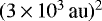
In the left panel of Fig. 2, we show the column density in a region of 3000 au × 3000 au in the yz-plane at t ≈ 43 kyr. The column density plot illustrates the presence of a bridge structure connecting sink A and sink B at this point in time. Briefly after the formation of sink B, the bridge-like structure emerges due to the compression of the filamentary arm seen in Fig. 1. During the approach of sink B to sink A, most of the mass inside the bridge region accretes onto sink A and sink B, leading to a lifetime of the bridge-structure of about ~ 10 kyr. In the right panel of Fig. 3, we show the velocity field with respect to the systemic velocity of sink A and sink B along the z-direction
 (1)
(1)
with MA and vA in addition to (MB) and (vB) being the mass and velocity of sink A and sink B, respectively. At this point in time (t = 43 kyr), the magnitude of the systemic velocity is |vsys|≈−1.1 × 104 cm s−1. Comparing the column density with the density-weighted velocity structure perpendicular to the plane (line-of-sight-velocity) shows that the bridge structures have at most modest line-of-sight velocities (vx < 104 cm s−1) with respectto the systemic velocity of sink A and sink B. That means that the bridge is kinematically quiescent along the line-of-sight at this point in time.
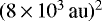
In Fig. 3, we show the same region as in the left panel of row 4 of Fig. 1, but 38 kyr later (i.e., 4 kyr before the formation of the second companion C). At this time, the primary A and companion B approach each other to form a binary system on the order of 100 au in separation with masses of MA ≈ 0.49 M⊙ and MB ≈ 0.25 M⊙ (see subsection below). Compared to the earlier time, the relatively broad gaseous arm (lower right in the yz-plane, left in the zx-plane, and upper part in the xy-plane of row 4 in Fig. 1) is denser and more pronounced due to compression. At this point in time, the projection along the x-axis again shows a bridge-like structure connecting the central binary system with the forming additional companion C. In general, the turbulent motions inherited from the GMC induce a rather complex velocity structure, in particular in the yz- and xy-planes. Following the dynamics of the system from t = t0[B] − 4 kyr snapshot until the formation of companion C, we see that the left part of the fork-like structure that is visible at the bottom right in the yz-projection in rows 2 and 3 of Fig. 1 merges with the longer arm. This compression contributes to the accumulation of mass in the arm that eventually leads to the formation of companion C.
Similar to the bridge shown in Fig. 2, it is also evident that the bridge shown in Fig. 3 is a result of the larger filamentary structure presented in Fig. 1. Looking at the line-of-sight velocity (vx) relative to the systemic velocity (right panel in Fig. 3) shows the variations of the velocity field in the surroundings. Although the velocity in the bridge has a mildly negative line-of-sight velocity (vx ~ −104 cm s−1), the plot nevertheless shows a transition from positive to negative velocities associated with the bended arm. The plot shows that bridges become kinematically quiescent once the flows with different orientation cancel each other out. In general, the dynamical history and evolution of the triple system demonstrate that bridge-like structures occur as a side-effect during the formation of multiple star systems.
3.3 Velocity structure
In this section, we present the velocity field around primary A during the early evolution, shortly before the formation of companion B. We plot the magnitude of the rotational velocity gas vϕ for all cells within a radial distance of r = 4000 au from the primary at t = 32 kyr, that is t = t0[B] − 4 kyr (Fig. 4). The color is used to display the density of each cell and the black dashed line shows the Keplerian velocity
 (2)
(2)
at this point in time for the sink mass of MA ≈ 0.29 M⊙, where G is the gravitational constant and r is the radial distance from the sink. At relatively small distances from the primary (r ≲ 100 au), the plot shows the approximately Keplerian profile (vϕ ∝ r−0.5) of the dense gas associated with the rotationally-supported disk. Cells with large deviations from the Keplerian profile at r ≲ 100 au have low densities and are not located in the midplane of the young disk. The disk truncates at a radius of r ~ 100 au as seen by the drop in density in the plot. However, by looking carefully at the diagram, one can see some cells at a distance of r ≈ 150 to 200 au of relatively enhanced density ρ > 10−12 g cm−3 and velocity magnitude v ≈ 105 cm s−1. In fact, this small characteristic is caused by the small gas stream visible in the lower right panel in Fig. 1. The velocity profile scaling slightly steeper than the Keplerian relation v ∝ r−0.5 is consistent with a gas parcel spiraling toward the central protostar.
Apart from that feature, the densities generally drop with increasing distance up to r ≈ 1000 au, where the gas accumulates to form the companion. In particular, one can see a wide spread in velocity magnitude (103 cm s−1 ≲ v ≲ 105 cm s−1) of the dense gas associated with the formation of companion B. Also accounting for the gas at lower densities ρ ≲ 10−15 g cm−3 at ≈ 3 × 10³ au shows an even larger spread of more than three orders of magnitude in velocity magnitude (3 × 102 cm s−1 ≲ v ≲ 7 × 105 cm s−1).
Analyzing the structure of the velocity field also shows the diversity of the orientation of the vector field. In Fig. 5 we illustrate the velocity orientation around companion B and companion C at the time of their formation, in detail, with respect to the systemic velocity. We plot the density distribution and velocity vectors around companion B (upper panels) and companion C (lower panels) in slices (2000 au)2 of the three planes spanned by the coordinate axes (left: yz-plane, middle: zx-plane, and right: yz-plane). The plots clearly show the different orientation of the velocity vectors leading to the compression that eventually causes the formation of the individual companions. Moreover, the velocity field in the xy-plane shows that the binary system of sink A and sink B moves toward the forming companion, thereby eventually sweeping up part of the material in the bridge.
In the following subsection, we analyze the formation process of the companion explicitly. We interpret the differences in velocities together with the abundance of filamentary structures as a consequence of the underlying turbulence present in the GMC cascading down to smaller scales.
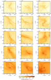 |
Fig. 1 Column density about 4 kyr before formation of first companion B in three planes of coordinate system (left: yz-plane, middle: zx-plane, right: xy-plane) on different scales (row 1: 512 × 103 au ≈ 2.5 pc, row 2: 128 × 103 au, row 3: 32 × 103 au, row 4: 8 × 10³ au, row 5: 2 × 10³ au). |
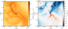 |
Fig. 2 Column density in yz-plane (left panel) and density-weighted velocity along x-axis relative to systemic velocity of young binary consisting of sink A and sink B (right panel) at time t = t0 (B) + 7 kyr = 43 kyr. The primaryis located at the center and the displayed area is |
 |
Fig. 3 Column density in yz-plane (left panel) and density-weighted velocity along the x-axis relative to systemic velocity of binary consisting of sink A and sink B (right panel) at time t = t0 (C) − 4 kyr = 70 kyr. The primaryis located at the center and the displayed area is |
 |
Fig. 4 Phase diagram illustrating cylindrically azimuthal velocity vϕ in cubical region of (8 × 10³ au)3 around primary about 4 × 10³ yr before formation of companion B. The rotational axis is chosen as the orientation of the angular momentum vector computed for a sphere around the primary A of radius 1000 au at this point in time. |
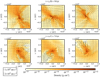 |
Fig. 5 Density distribution at time t = tB,0 of formation of first companion B (upper panels) and formation of second companion C at t = tC,0 (lower panels). The panels show slices of the three planes spanned by the coordinate system (left: yz-plane, middle: zx-plane, and right: xy-plane) with the position of the forming sink at the center. The arrows show the velocity with respect to the systemic velocity in the corresponding plane for every 50th data point in the plane. The length of the arrows scales linearly with the velocity magnitude. In the lower left corner, the length corresponding to 105 and 2 × 105 cm s−1 is shown. |
3.4 Formation of companions
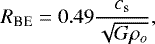
The critical radius of an isothermal sphere supported by gas pressure against gravitational collapse, that is a Bonnor-Ebert sphere, is given by
 (3)
(3)
where cs is the sound speed, G is the gravitational constant, and ρo is the outer density (Ebert 1955; Bonnor 1956). As a convenient estimate of RBE in practical units, one can use
![Mathematical equation: \begin{equation*} \left[\frac{R_{\textrm{BE}}}{\,{\rm\,pc}} \right]= 1.88 \left[\frac{T}{\,\textrm{K}} \right]^{0.5} \left[\frac{n}{\,\textrm{cm}^{-3}}\right]^{-0.5}, \end{equation*}](/articles/aa/full_html/2019/08/aa35504-19/aa35504-19-eq8.png) (4)
(4)
which would yield a radius of about 104 au assuming a number density of 104 cm−3 < n < 105 cm−3 and temperature T = 10 K. This is considered typical for rough calculations of the collapse of a solar mass star. It is evident that the formation of both companions deviates from such a classical collapse scenario for single stars, as also indicated by the relatively small collapsing region of only ~100 au just at the location where the individual companions form. Instead, the companions form rather as a consequence of turbulent fragmentation inside the elongated heavily perturbed prestellar core, which is similar to what has been seen in dedicated core collapse simulations with turbulence (e.g., Seifried et al. 2013).
In the following, we investigate the formation of the first companion in more detail. Shortly after formation of the primary A, gas predominantly approaches the sink from within the filament, resulting in non-isotropic accretion. Given that the inflowing gas has angular momentum with respect to the star, not all of the gas in the flow accretes onto the protostar. Instead, part of the gas is deflected by the gravitational field of the protostar and passes by the protostar. However, gas also approaches the protostar from the opposite direction and hence compresses the gas to form companion B at a distance of ≈ 1500 au from the primary (seeaccumulation of gas in the projection plots in Fig. 1 and in the slice plots, upper panel Fig. 5).
Following the system further in time, the two stars approach and orbit each other eccentrically with a separation between ≲ 100 au and ~300 au. While this happens, gas also passes by the primary star and gets compressed in a dense arm similar to the scenario before the formation of the first companion (see Fig. 3). As a consequence of this, the second wide companion C forms at a distance of about 2100 au from the close binary system.
To give a better overview of the evolution of the gas contributing to the formation process of the three different stars, we show maps of the column density of size (1.6 × 10⁴ au)2 along the three coordinate axes for fourdifferent times (t = 20 kyr, t = 50 kyr, t = 70 kyr, and t = 90 kyr after the formation of the primary) in Fig. 6. The maps are centered at the location of the primary and the dots in the plot represent gas that is located within 30 au at t = 90 kyr from the primary A (black dots), secondary B (blue dots), and tertiary C (red dots). Using tracer particles, we can constrain the origin of the accreting gas for the individual sinks. The figure clearly illustrates that most of the material accreting onto the triple system is indeed located in the dense filamentary arm.
In Fig. 7, we plot how far away the gas, that is located within 100 au from sink A (upper panel) and sink B (lower panel) at Δt = 10(30, 50, 86) kyr after sink formation (tform), was located at tform. The plot demonstrates that both sinks initially accrete the collapsing gas in their vicinity of ~1000 au. However, at later times, a significant fraction of the mass stems from distances initially several 1000 au from the sinks. Gas accreting from distances beyond the scale of a Bonnor-Ebert sphere is inconsistent with the expected accretion pattern of traditional core collapse models. However, consistent with observations, the sinks form in elongated filaments. As shown in Figs. 6 and 7, accretion inside these filamentary birth environments allows stars to accrete gas from initially far distances.
Moreover, Fig. 6 shows that all of the three objects share the same reservoir, although the reservoir of companion C is a bit more distinct. This is not surprising, considering that companion C is the youngest and least massive of the three objects. Furthermore, as illustrated in Fig. 8, sink B approaches sink A during the evolution and the two sinks accrete gas as a binary system of smaller separation for some time before the formation of companion C at a larger distance from the, by then, relatively close binary system of separation ~100 au. The sinks initially have the largest separation in the z-direction (magenta solid line for ΔzAB and green dashed line ΔzAC in Fig. 8), which reflects the fact that the filamentary arm is predominantly oriented along the z-axis. The separation between both companions from the primary is initially largest before the sinks approach each other. In particular, companion C and the binary star consisting of A and B approach each other faster than companion B approaches A after its formation. This is due to the stronger gravitational interactions between the sinks. At the time of formation of companion C t0,C, the mass of primary A (MA(t0,C) ≈ 0.49 M⊙) together with the additional mass of companion B (MB(t0,C) ≈ 0.26 M⊙) in the vicinity of A corresponds to a higher gravitational potential than at the earlier time of formation of companion B t0,B, where the primary had a mass of MA(t0,B) ≈ 0.29 M⊙.
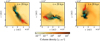 |
Fig. 6 Column density in three planes of coordinate system (width: 1.6 × 10⁴ au; left: yz-plane, middle: zx-plane, right: xy-plane) at time t = 20 × 103 yr after formation of primary A. The colored dots illustrate the origin and dynamics of accreting gas of the individual sinks. Black (cyan, red) dots represent particles that are located within a distance of 30 au from the primary A (B, C) at t = 90 × 103 yr. |
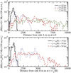 |
Fig. 7 Origin of gas for sink A and sink B at t = 10 kyr (black solid line), t = 30 kyr (blue dotted line), 50 kyr (red dashed line), and t = 86 kyr (green dashed-dotted line) after formation of individual sinks. |
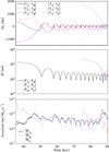 |
Fig. 8 Evolution of distance between different objects of multiple stellar system. Upper panel: difference between sink A and B in x (black solid line), y (red dashed line), and z (magenta solid line), as well as the difference between sink A and C in x (blue dotted line), y (cyan dash-dotted line), and z (green dashed line). Middle panel: absolute distance r between sinks A and B (black solid line), sinks A and C (blue dotted line), and sinks B and C (red dashed line). Lower panel: accretion profile for the three sinks involved from t = 35 × 103 yr to t = 90 × 103 yr after formation of the primary. The black solid line represents the primary A, the blue dotted line corresponds to companion B, and the red dashed line corresponds to companion C. |
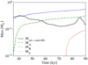 |
Fig. 9 Evolution of mass located within distance of 1000 au from center of mass of primary and secondary (black solid line), mass of sink A (blue dashed line), mass of sink B (green dashed-dotted line), and mass of sink C (red dotted line). |
3.5 Accretion and evolution of the protostellar multiple
By investigating the accretion profile of the different sinks (lower panel of Fig. 8), we see a direct effect of the dynamics on the accretion process of the sinks. Focusing on the profile of companion A and B first, the accretion rate of the primary increases when companion B comes closer. Later, the eccentric orbits of companion B around A cause a periodic pattern in the accretion rates of both primary A and companion B. A similar effect is also evident when the second companion approaches the binary system consisting of A and B. To understand the accretion process more clearly, we plot the evolution of mass that is enclosed within a radius of 1000 au from the center of mass of the primary and the secondary
 (5)
(5)
where mA (mB) represents the mass of the primary A (secondary B) and rA (rB) corresponds to the position of the primary A (secondary B) in Fig. 9. The plot shows an increase in enclosed mass around the binary system for the approach of companion C, as seen in Fig. 8. Hence, the mass reservoir for accretion onto the binary system of sink A and B is refueled, thus leading to the increase in the accretion rate seen in the lower panel of Fig. 8. In contrast, the less massive approaching sink now has to share its mass reservoir with the already established binary system, and hence its accretion rate drops. Quantitatively, when the tertiary star approaches the system at a distance of about 200 au, its accretion rate decreases from about Ṁ ≈ 6 × 10⁻⁶ M⊙ yr−1 to less than 10−6 M⊙ yr−1 within less than 1 kyr, while the accretion rates of companion B and especially primary A increase by up to a factor of ten within only a few kyr.
Our results show the importance of dynamical interactions on the accretion process of young, deeply embedded protostars. Without thepresence of gas during this stage, the migration process of the companion(s) would be free of dissipation due to the lack of accretion. Consequently, the secondary B would approach and leave the primary again on a hyperbolic trajectory. However, the two stars are still deeply embedded. The surrounding gas has a dissipative effect on the secondary through gas accretion during migration toward the primary. Using smoothed particle hydrodynamics (SPH) simulations, Bate & Bonnell (1997) carried out a parameter study for accreting circular binary systems with constant infalling specific to angular momentum, demonstrating that the separation of binaries decreases even if the specific angular momentum of the infalling gas is much larger than the specific angular momentum of the binary.
The focus of this work is on the morphology of the bridge structure during stellar multiple formation. Furthermore, an in-depth analysis of the evolution of binary separation and angular momentum transfer is beyond the scope of this paper. However, consistent with previous models (Bate & Bonnell 1997; Offner et al. 2010), our results suggest a characteristic sequence for the formation process of multiple stellar systems. First, the primary forms as a consequence of gravitational collapse in a deformed prestellar core. Subsequently, the secondary forms in the filamentary arm connected to the primary due to contraction of mass at distances of ≳ 1000 au induced by the underlying turbulence in the GMC. The formation at such distances is consistent with an observed peak at ~3000 au for YSO Class 0 objects in Perseus (Tobin et al. 2016a). Afterwards, induced by the gravitational potential of the relatively massive primary, the secondary migrates toward the primary. In the final stage, the secondary is captured by the primary and forms an eccentric binary system with characteristic separation of ~100 au due to the interaction of gravity and accretion. Again, such a separation is consistent with the observed peak in the distribution of protostellar separation for Class 0 and even more for Class I objects (Tobin et al. 2016a). Considering subsequent components, our models suggest the same initial sequence as for the secondary. However, different to the two-body scenario, tidal interactions in the three-body system also imply dissipation that can possibly lead to capturing of companions even without any gas. One of the components is possibly ejected during the interaction, potentially leading to the formation of binary systems with smaller separation.
4 Discussion
In this section, we discuss the consequences of our results. First, we discuss the robustness of the sequential formation of protostellar multiples by turbulent fragmentation in our model. We, furthermore, discuss the dynamical evolution of the protostellar multiples and the limitations in our model. Finally, we compare the bridge-structures seen in our model with recent observations of bridge- and arc-structures associated with different protostellar sources.
4.1 Constraining the origin of protostellar companions
There are two suggested mechanisms for the formation of stellar multiples: disk fragmentation (Adams et al. 1989; Kratter et al. 2010) and turbulent fragmentation (Padoan 1995; Padoan & Nordlund 2002; Offner et al. 2010). Per definition, the former can only occur in protostellar disks, that is on scales of ≲ 100 au, while turbulent fragmentation predominantly acts on larger scales of ≳1000 au. Although statistical constraints of main-sequence stellar binaries and multiplicities have been known for decades (Duquennoy & Mayor 1991), only recently has it become feasible to constrain multiplicity during the protostellar phase. Using the Karl G. Jansky Very Large Array (VLA), Tobin et al. (2016a) provide constraints on the multiplicity fraction during the protostellar phase for Class 0 and Class I YSOs in Perseus. The survey shows a bimodal distribution for the protostellar separation in the Class 0 with a peak at ~75 au and another peak at ~3000 au. The authors attribute the inner peak to disk fragmentation and the outer peak to turbulent fragmentation, though they also acknowledge that the lower number of binaries with separation of ≳ 1000 au for Class I might be a consequence of inward migration of companions formed by turbulent fragmentation. To properly constrain the formation mechanism, computationally expensive models accounting for the turbulence in the ISM are necessary.
The selected primary forms as a consequence of gravitational collapse of dense gas within a perturbed core structure. In contrast, the formation of the companions occurs inside the gaseous arms that are connected to the primary in a different manner. Tracing the evolution at the location close to sink formation, we see that their formation may be understood as a consequence of colliding flows for both companions. The gas inside the long filamentary arm feeds the star, while the velocity field around it has a different orientation, and hence compresses the gas enough to cause sink formation. One may wonder whether the sink only forms because of insufficient resolution of the angular momentum present in the flow structure at ≈ 2 au resolution. To test the robustness of sink formation, we conducted comparison runs with lref = 23(24,25,26,27), corresponding to minimum cell sizes of ≈1 (≈ 0.5, ≈ 0.23, ≈ 0.123, ≈ 0.061 au) as shown in the appendix. We confirm the formation of the sink in all of these comparison runs, thus demonstrating the robustness of companion formation.
4.2 Dynamical evolution of the protostellar companions
Recently, Muñoz et al. (2019) thoroughly carried out 2D hydrodynamical simulations with the moving mesh code AREPO (Springel 2010) of an accreting equal-mass binary. In contrast to our results, they find an increase in stellar separation a rather than a decrease; the increase in separation is ≈5× stronger for the circular case than for the eccentric case e = 0.6. However, their setup is quite different from our zoom-in setup. In our simulations the companion forms in its turbulent birth environment, where it is initially unbound, and gets captured by the primary at a later stage of evolution. In contrast, their simulations start with a binary star that is already in a bound state, and which evolves for many more orbits (Norbit = 3500) in an idealized 2D setup. Moreover, our results account for the effects of magnetic fields that can transfer angular momentum away from the gas close to the star. Therefore, it is difficult to directly compare our results of a young forming protostellar binary with the longer term evolution of an already existing binary system in a less violent environment. Another significant difference between our scenario and a scenario of an already established binary system is the change in mass ratio of the binary components. As Muñoz et al. (2019) pointed out, the mass ratio in their setup is q = 1, whereas in our scenario the ratio varies and quickly increases, briefly after the formation of companion B.
For a conceptual understanding of the effects of mass ratio q and mass accretion rate of the binary Ṁb, we discuss the fiducial case of an accreting circular binary as analyzed in detail by (e.g., Bate & Bonnell 1997). Taking the time derivative of the angular momentum around its center of mass
 (6)
(6)
and solvingit for the time derivative of binary separation ȧ yields
 (7)
(7)
According to
 (8)
(8)
a drastic decrease in mass ratio corresponds to a shrinking binary separation. Together with the effect of mass accretion
 (9)
(9)
the binary separation is expected to shrink most significantly, briefly after the formation of the companion and before the change in separation becomes milder, when  and Ṁ decrease.
In fact, our results are in good agreement with results from 3D MHD simulations using FLASH (Fryxell et al. 2000) explicitly considering the protostellar regime (Kuruwita et al. 2017). Starting from idealized spherical cloud conditions Kuruwita et al. (2017) find a quick decrease in binary separation during the early accretion phase of the binary, which is similar to our results.
4.3 Limitations of the model
4.3.1 Single model run
Considering the evolution of the binary and triple system, our results show a sequence of protostellar multiples involving turbulent fragmentation and protostellar migration. However, we only analyzed a single system with a modest resolution using a minimum cell size of initially Δx ≈ 2 au, and mostly Δx ≈ 2 au for the densest gas. Carrying out comparison runs, with a broad appliance of higher resolution for a longer time than only testing the formation of the companions, is currently too expensive computationally.
4.3.2 Outflows and sink implementation
Outflows are driven mostly on scales of 1 to 10 au (Bacciotti et al. 2002; Bjerkeli et al. 2016), and we, at best, barely resolved mass loss via jets or winds and lack the corresponding feedback (Wang et al. 2010; Cunningham et al. 2018). Nevertheless, to account for the mass loss, we simply reduced the mass that accretes onto the sinks by a factor of two. Given that the evolution of a multiple system depends on the mass accretion rate as well as on the mass ratios of the different components, a thorough analysis of the early evolution of multiple stellar systems requires higher resolution as well as a careful treatment of the accretion onto the sink. For an analysis and discussion of the sink settings and their effect on the formation of stellar multiples, please refer to Haugbølle et al. (2018). Furthermore, the dynamics of multiples with a separation of ≲ 100 au are also affected by the individual disks of the different components. With our current resolution, we can only roughly account for disks. Finally, our results based on one multiple system can only be suggestive. Constraining the distribution of protostellar separation in detail requires a larger sample of objects.
4.3.3 Magnetic fields and non-ideal MHD effects
Regarding magnetic fields, a short-coming of our simulations is the assumption of ideal MHD, and the corresponding negligence of physical resistivities corresponding to Ohmic dissipation, ambipolar diffusion, and the Hall effect (see e.g., Tomida et al. 2015; Tsukamoto et al. 2015; Masson et al. 2016; Wurster et al. 2018). Similar to previous spherical collapse simulations that solve the equations of ideal MHD (Seifried et al. 2011; Joos et al. 2012), the pile-up of magnetic pressure during the stellar collapse phase causes outward motions of gas away from the sink. Although these magnetic bubbles can lead to compression of gas around the sinks (Vaytet et al. 2018), the formation of the arcs – and eventually the companions – are ultimately caused by the turbulent dynamics present in the protostellar environment. Nevertheless, we aim to avoid potentially spurious effects induced by the magnetic interchange instability by accounting for non-ideal MHD effects in future simulations with the code framework DISPATCH (Nordlund et al. 2018).
4.3.4 Radiative transfer
In our model, we model the thermodynamics with a heating and cooling table though the recipe that typically causes quasi-isothermal conditions (T ≈ 10 K) for the densest gas responsible for star formation. A more sophisticated treatment of the thermodynamics would provide additional thermal support against fragmentation. First, the compression of gas itself induces some heating that we most likely underestimate. However, considering that the collapse phase finalizing companion formation occurs on spatial scales of only a few 102 au (cf. Fig. 5), we doubt that additional thermal pressure support would counteract the compression acting on the large-scale sufficiently. Second, by accounting for the irradiation from nearby stars (e.g., Geen et al. 2015), the primary star by using a radiative transfer implementation (Rosdahl et al. 2013; Rosdahl & Teyssier 2015; Frostholm et al. 2018) would heat up the gas in the region around the protostar in particular.
Considering an optically thin environment, the temperature induced by the protostar irradiating as a perfect black body follows
 (10)
(10)
where L is the luminosity, σSB is the Stefan-Boltzmann constant, and r is the radial distance from the protostar. Hence, the temperature would drop with increasing radial distance from the star as T ∝ r−0.5. The luminosity of a protostar in its early stage is predominatly determined by the accretion rate. With an accretion rate of Ṁ = 10−5 M⊙ yr−1 and given a commonly assumed protostellar radius of R = 3 R⊙ (Stahler 1988) with mass M = 0.5 M⊙, its luminosity according to
 (11)
(11)
is Lacc ≈ 50 L⊙. This rough approximation shows that even for the highest accretion rates, when the primary has a mass of M ≈ 0.5 M⊙, protostellar heating would only modestly increase the temperature beyond 1000 au distances toless than 30 K. For future studies investigating the processes on smaller distances r < 10 au, however, protostellar heating and radiative transfer are essential.
4.4 Comparison with observed arcs and bridges
In our model, the most outstanding bridge-structure (see upper panel Fig. 3) occurs a few kyr before the formation of the third companion. The arc connects companion B – by that time only ~100 au away from the primary – with the blob that leads to the formation of companion C at a projected distance of about 2000 au. The arc resembles a bended bridge with a kinematically mild velocity structure compared to its surroundings. However, we also see another shorter lived ≲ 1000 au kinematically quiescent bridge-like structure at earlier times (t ≈ tB,0 + 10 kyr) connecting the primary A with the secondary B in Fig. 2. The synthetic bridge shown in Fig. 2 is about 1000 au in length. The synthetic bridge shown in Fig. 3 extents to about 2000 au and involves three protostellar sources altogether. Our modeled structure shows several features that are in good agreement with observed arc- and bridge-like structures.
Bridge- or arc-like structures have been reported for several deeply embedded sources. One of the most prominent examples of an observed bridge-like structure is the case of the young binary IRAS 16293, where the two sources are connected by an arc-like filament. The two protostars have a projected distance of 705 au indicating formation via turbulent fragmentation such as is seen in our models. The bridge in IRAS 16293 is kinematically quiescent, while the surrounding is kinematically active (Oya et al. 2018; van der Wiel et al. 2019). This is similar to the bridge-like structure in our model of the forming triple system. Another arc structure is seen for the Class I system IRAS 04191+1523, where a bridge connects the two binary components (projected separation of 860 au). Using C18 O as a kinematic tracer, Lee et al. (2017) also favor a scenario where the system formed via turbulent fragmentation.
Different from our triple system, IRAS 04191+1523 consists of only two protostellar components. However, bridge- and arc-structures are also observed for protostellar multiples of higher order than binary. For IRAS 16293, it is debated whether source A is in fact a single protostar (Wootten 1989; Chandler et al. 2005), a tight binary (Loinard et al. 2007; Pech et al. 2010), or even a tight triple system (Hernández-Gómez et al. 2019) with strong jet components (Kristensen et al. 2013; Girart et al. 2014; Yeh et al. 2008). A confirmed triple system is the case of SR24 (Fernández-López et al. 2017), which consists of a close binary SR24N with a separation of only ~10 au (Correia et al. 2006) and a third component with a separation of more than 620 au. Another striking example of a bent filamentary arm in a triple system is the case of L1448 IRS3B (Tobin et al. 2016b). With projected separations from the primary of the first companion of 61 and 183 au of the second companion, the system is more compact than our model as well as the binary systems IRAS 16293 and IRAS 04191+1523. Tobin et al. (2016b) show that this system may have been a result of disk fragmentation rather than turbulent fragmentation on larger scales. However, protostellar companions may subsequently migrate as the velocity profile of a multiple system continuously becomes more Keplerian during the capturing phase (Bate et al. 2002). Therefore, L1448 IRS 3B and SR24 – even involving its close binary SR24N – may nevertheless have formed via turbulent fragmentation in a similar manner as the wide triple system in our case study.
While most of the observations mentioned above show evidence of bridge structures connecting already formed protostars, the bridge in our model already exists. Additionally, it is in fact most outstanding prior to the formation of the third companion. This is consistent with observations of prominent arc-structures observed for other embedded sources.
The two components of IRAS 16293 have been shown to have differences which could be attributed to differences in age. The lack of outflows from source B and prominent outflows observed from source A, have been suggested as a sign that source A is the more evolved object (e.g., Pineda et al. 2012; Loinard et al. 2013; Kristensen et al. 2013). Other indicators, such as chemical differentiation between the sources could also be attributed to age differences, although these differences would indicate source B to be the more evolved source (see Calcutt et al. 2018a,b for a discussion).
In tracing HCO+, Tokuda et al. (2014) observed an arc-structure for L1521F extending from source MMS1 to a distance of ~2000 au with features of small dense cores located in the arc. Considering that the second synthetic bridge-structure is most pronounced before the small core has collapsed to form companion C, we expect dispersal of the arc seen in L1521F over the next few ~10 kyr. Pineda et al. (2015) demonstrate the presence of filamentary structures on scales of ~1000 au around at least one embedded protostar located in the dense core Barnard 5. Their observations show the presence of three density enhancements in these filamentary arms. Given the abundance of filamentary structures accompanying star formation in our model, our results support the interpretation that these density enhancements are associated with prestellar condensates.
Recently, Sadavoy et al. (2018) measured dust polarization in IRAS 16293 to study the morphology of the underlying magnetic field. Analyzing the magnetic field structure in our synthetic bridges is of high interest, but it is beyond the scope of this paper. Dust polarization depends on the active mechanism of aligning the dust grains, which is rather complex to model in such a dense and turbulent environment. Therefore, instead of providing an oversimplified polarization map based on the magnetic field structure, we will present the work of careful synthetic dust polarization measurements with the radiative transfer tool POLARIS (Reissl et al. 2016) in an upcoming paper.
Taking into account all of the above observations, a picture emerges, in which arcs and bridges occur at different evolutionarystages of the formation of protostellar multiples. The temporary appearance of arc- and bridge-structures in our model are consistent with the observations. Our zoom-in model demonstrates that kinematically quiescent bridge-structures are transient phenomena induced by the turbulent motions involved in the formation process of stellar multiples. Our analysis suggests lifetimes of the observed structures on the order of up to a few 104 yr. Although this may seem to be rather short, our model suggests that these structures are common features of the formation of stellar multiples. Therefore, we expect to observe more bridge-like structures around other Class 0 objects in the case of a duration of the Class 0 phase of approximately 105 yr and giventhat multiple bridge structures can occur during the formation of a protostellar multiple, as shown in this paper. Considering that >50% of Class 0 systems appear to be multiples (Tobin et al. 2016a), and by taking into account the lifetimes of the Class 0 phase of ≈ 105 yr and the lifetime of the bridges of ~104 yr, we expect to see a bridge-like structure in >5% of Class 0 protostars.
5 Conclusion
Using zoom-in simulations, we analyze the formation process of a triple-star system embedded in the turbulent environment of a magnetized GMC. The first companion B forms at t ≈ 35 kyr after the primary A, at a distance of about 1500 au from the primary, and the tertiary C forms at a distance of about 2100 au from the, by then, more narrow binary system (rAB ~100 au), about 75 kyr after primary A formed. Both companions form as a consequence of compression induced by colliding flows associated with turbulent fragmentation in the interstellar medium. Our model shows the following sequence for the formation of protostellar multiples: the protostellar companions initially form with a wide separation from the primary (~1000 au) via turbulent fragmentation, afterward they migrate inward to distances of ~100 au on timescales of Δt ~ 10 kyr before they are captured and bound in eccentric systems of protostellar multiples. Once the system is bound, the accretion profiles of the young protostars are variable related to the periodic pattern of the orbital frequency of the system.
We find transient filamentary arms connecting two protostars that build as a by-product of the formation process of the companions. These bridges persist for time-scales on the order of Δt ~ 10 kyr. Studying the properties of these bridges more closely shows no sign of a preferred motion toward any of the protostellar components. Instead, the velocity components of the colliding flows cancel each other out and the bridge becomes kinematically quiescent, similar to what has recently been observed in systems such as IRAS 16293–2422 (van der Wiel et al. 2019).
Considering the velocity components, our analysis shows that bridge-structures are a consequence of compression due to flows acting on larger scales, partly canceling out the velocity components in the compressed region forming the bridge. In this way, the gas located inside the bridge can become kinematically rather quiescent compared to the systemic velocity. With respect to the accretion process of the companions, the bridge structure acts as an important mass reservoir of the different stellar components. Using tracer particles, we analyze the origin of the gas accreting onto the different components. The analysis shows firstly that the different protostellar components share the same mass reservoir, at least partly, and secondly that the protostellar companions are fed by the gas located in the elongated compressed filament.
Therefore, the gas located in the bridge eventually contributes to protostellar accretion in the system, but it is different from a gas stream feeding one individual source. While the gas in streams actively approaches a single star from one direction, the gas located in the bridge is available to be picked up by any star in the system. Gas located in different parts of the bridge can accrete onto one of the sources, and hence the bridge may consist of gas streams with flow directions toward different sources.
In this paper, we aimed for a deeper understanding of the origin of arc- and bridge-like structures observed for multiple embedded protostars. In particular, it is difficult to understand the origin of quiescent dense structures (e.g., IRAS 16293-2422) with a picture of isolated star formation in mind. However, when accounting for the overall dynamics in the turbulent GMC, the results bring to light that such structures are induced by the underlying turbulent motions in the GMC. Our model demonstrates that bridge-like structures occur as natural transient phenomena associated with the formation of protostellar multiples via turbulent fragmentation. Against the background of observed arc- and bridge-like structures associated with protostellar multiples, our results strongly indicate age differences of Δt ~ 10 kyr between the different components of the multiple. Future kinematic studies of young protostars in bridge structures will help to test this result.
Acknowledgements
We thank the anonymous referee for their insightful and constructive comments on an earlier draft of the manuscript that helped to improve the quality of this paper. We thank Troels Haugbølle and Åke Nordlund for their development of the zoom-in technique for the modified version of RAMSES. M.K. thanks the developers of the python-based analyzing tool YT http://yt-project.org/ (Turk et al. 2011), which simplified the analysis significantly. Furthermore, M.K. thanks Kees Dullemond for insightful discussions. The research of M.K. is supported by a research grant of the Independent Research Foundation Denmark (IRFD) (international postdoctoral fellow, project number: 8028-00025B). We acknowledge PRACE for awarding access to the computing resource CURIE based in France at CEA for carrying out part of the simulations. Thanks to a research grant from Villum Fonden (VKR023406), M.K. could use archival storage and computing nodes at the University of Copenhagen HPC centre to carry out essential parts of the simulations and the post-processing. M.K. acknowledges the support of the DFG Research Unit “Transition Disks” (FOR 2634/1, ER 685/8-1). The research of LEK is supported by a research grant (19127) from VILLUM FONDEN. Research at the Centre for Star and Planet Formation is funded by the Danish National Research Foundation.
Appendix A Formation of companions at higher resolution
Stars form as a consequence of gravitational collapse. In our numerical scheme, we account for these properties by requiringgas to be above a given density threshold as well as the gas in the cell, that is infalling gas ∇ ⋅ v < 0. In a dense turbulent medium, using low resolution averages out the deviations of the velocity field. As a consequence, sinks that form at low resolution, may not form at a higher resolution when accounting for the velocity deviations. As mentioned in the text, the system forms in a turbulent medium with fluctuating velocities. To test whether the formation of the companions is robust, we conducted comparison runs with higher resolution in the regions, where companion B or C form. For the test, we used lref = 22(23,24,25, 26,27), corresponding to minimum cell sizes of ≈2 au (≈ 1, ≈ 0.5, ≈ 0.23, ≈ 0.123, ≈ 0.061 au). As shown inFig. A.1, sink formation is triggered in the higher resolution runs, demonstrating that the sinks indeed form due to a local collapse on smaller scales triggered by the colliding flows acting on larger scales. Sinks form later when using higher resolution because the density to trigger sink formation is a multiple of the cell density at highest level. The density threshold for triggering the formation of a sink is 10 × ρc, where ρc is the density threshold for resolving a cell to highest resolution. To form a sink, the threshold density has to be refined with at least 25 cells. As the densities increase during protostellar collapse with evolving time, applying higher resolution therefore delays the creation of the sink particle. However, for the refinement levels considered here, the delay is < 1 kyr, and hence negligible for our analysis of the evolution on time scales of up to 100 kyr (see also Kuffmeier et al. 2017).
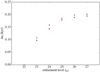 |
Fig. A.1 Time of formation of sinks A (blue asterisks) and B (red triangles) using differentmaximum resolution with respect to sink formation using resolution of lref = 22 corresponding to minimum cell size of 2 au. |
References
- Adams, F. C., Ruden, S. P., & Shu, F. H. 1989, ApJ, 347, 959 [NASA ADS] [CrossRef] [Google Scholar]
- André, P., Men’shchikov, A., Bontemps, S., et al. 2010, A&A, 518, L102 [NASA ADS] [CrossRef] [EDP Sciences] [Google Scholar]
- Bacciotti, F., Ray, T. P., Mundt, R., Eislöffel, J., & Solf, J. 2002, ApJ, 576, 222 [NASA ADS] [CrossRef] [Google Scholar]
- Bate, M. R., & Bonnell, I. A. 1997, MNRAS, 285, 33 [NASA ADS] [CrossRef] [Google Scholar]
- Bate, M. R., Bonnell, I. A., & Bromm, V. 2002, MNRAS, 332, L65 [NASA ADS] [CrossRef] [Google Scholar]
- Bjerkeli, P., van der Wiel, M. H. D., Harsono, D., Ramsey, J. P., & Jørgensen, J. K. 2016, Nature, 540, 406 [NASA ADS] [CrossRef] [Google Scholar]
- Bonnor, W. B. 1956, MNRAS, 116, 351 [CrossRef] [Google Scholar]
- Calcutt, H., Fiechter, M. R., Willis, E. R., et al. 2018a, A&A, 617, A95 [NASA ADS] [CrossRef] [EDP Sciences] [Google Scholar]
- Calcutt, H., Jørgensen, J. K., Müller, H. S. P., et al. 2018b, A&A, 616, A90 [NASA ADS] [CrossRef] [EDP Sciences] [Google Scholar]
- Chandler, C. J., Brogan, C. L., Shirley, Y. L., & Loinard, L. 2005, ApJ, 632, 371 [NASA ADS] [CrossRef] [Google Scholar]
- Chen, X., Arce, H. G., Zhang, Q., et al. 2013, ApJ, 768, 110 [NASA ADS] [CrossRef] [Google Scholar]
- Connelley, M. S., Reipurth, B., & Tokunaga, A. T. 2008, AJ, 135, 2496 [NASA ADS] [CrossRef] [Google Scholar]
- Correia, S., Zinnecker, H., Ratzka, T., & Sterzik, M. F. 2006, A&A, 459, 909 [NASA ADS] [CrossRef] [EDP Sciences] [Google Scholar]
- Cunningham, A. J., Krumholz, M. R., McKee, C. F., & Klein, R. I. 2018, MNRAS, 476, 771 [NASA ADS] [CrossRef] [Google Scholar]
- Duquennoy, A., & Mayor, M. 1991, A&A, 248, 485 [NASA ADS] [Google Scholar]
- Dzib, S. A., Ortiz-León, G. N., Hernández-Gómez, A., et al. 2018, A&A, 614, A20 [NASA ADS] [CrossRef] [EDP Sciences] [Google Scholar]
- Ebert, R. 1955, Z. Astrophys., 37, 217 [NASA ADS] [Google Scholar]
- Ferland, G. J., Korista, K. T., Verner, D. A., et al. 1998, PASP, 110, 761 [Google Scholar]
- Fernández-López, M., Zapata, L. A., & Gabbasov, R. 2017, ApJ, 845, 10 [NASA ADS] [CrossRef] [Google Scholar]
- Fromang, S., Hennebelle, P., & Teyssier, R. 2006, A&A, 457, 371 [NASA ADS] [CrossRef] [EDP Sciences] [Google Scholar]
- Frostholm, T., Haugbølle, T., & Grassi, T. 2018, ArXiv e-prints [arXiv:1809.05541] [Google Scholar]
- Fryxell, B., Olson, K., Ricker, P., et al. 2000, ApJS, 131, 273 [NASA ADS] [CrossRef] [Google Scholar]
- Geen, S., Hennebelle, P., Tremblin, P., & Rosdahl, J. 2015, MNRAS, 454, 4484 [NASA ADS] [CrossRef] [Google Scholar]
- Girart, J. M., Estalella, R., Palau, A., Torrelles, J. M., & Rao, R. 2014, ApJ, 780, L11 [NASA ADS] [CrossRef] [Google Scholar]
- Gnedin, N. Y., & Hollon, N. 2012, ApJS, 202, 13 [NASA ADS] [CrossRef] [Google Scholar]
- Haugbølle, T., Padoan, P., & Nordlund, Å. 2018, ApJ, 854, 35 [NASA ADS] [CrossRef] [Google Scholar]
- Hernández-Gómez, A., Loinard, L., Chandler, C. J., et al. 2019, ApJ, 875, 94 [NASA ADS] [CrossRef] [Google Scholar]
- Joos, M., Hennebelle, P., & Ciardi, A. 2012, A&A, 543, A128 [NASA ADS] [CrossRef] [EDP Sciences] [Google Scholar]
- Kratter, K. M., Matzner, C. D., Krumholz, M. R., & Klein, R. I. 2010, ApJ, 708, 1585 [NASA ADS] [CrossRef] [Google Scholar]
- Kristensen, L. E., Klaassen, P. D., Mottram, J. C., Schmalzl, M., & Hogerheijde, M. R. 2013, A&A, 549, L6 [NASA ADS] [CrossRef] [EDP Sciences] [Google Scholar]
- Kuffmeier, M., Frostholm Mogensen, T., Haugbølle, T., Bizzarro, M., & Nordlund, Å. 2016, ApJ, 826, 22 [NASA ADS] [CrossRef] [Google Scholar]
- Kuffmeier, M., Haugbølle, T., & Nordlund, Å. 2017, ApJ, 846, 7 [NASA ADS] [CrossRef] [Google Scholar]
- Kuffmeier, M., Frimann, S., Jensen, S. S., & Haugbølle, T. 2018, MNRAS, 475, 2642 [NASA ADS] [CrossRef] [Google Scholar]
- Kuruwita, R. L., Federrath, C., & Ireland, M. 2017, MNRAS, 470, 1626 [NASA ADS] [CrossRef] [Google Scholar]
- Larson, R. B. 1969, MNRAS, 145, 271 [NASA ADS] [CrossRef] [Google Scholar]
- Larson, R. B. 1981, MNRAS, 194, 809 [NASA ADS] [CrossRef] [Google Scholar]
- Lee, J.-E., Lee, S., Dunham, M. M., et al. 2017, Nat. Astron., 1, 0172 [NASA ADS] [CrossRef] [Google Scholar]
- Liu, H. B., Takami, M., Kudo, T., et al. 2016, Sci. Adv., 2, e1500875 [Google Scholar]
- Loinard, L., Chandler, C. J., Rodríguez, L. F., et al. 2007, ApJ, 670, 1353 [NASA ADS] [CrossRef] [Google Scholar]
- Loinard, L., Zapata, L. A., Rodríguez, L. F., et al. 2013, MNRAS, 430, L10 [NASA ADS] [CrossRef] [Google Scholar]
- Looney, L. W., Mundy, L. G., & Welch, W. J. 2000, ApJ, 529, 477 [NASA ADS] [CrossRef] [Google Scholar]
- Masson, J., Chabrier, G., Hennebelle, P., Vaytet, N., & Commerçon, B. 2016, A&A, 587, A32 [NASA ADS] [CrossRef] [EDP Sciences] [Google Scholar]
- Mundy, L. G., Wootten, A., Wilking, B. A., Blake, G. A., & Sargent, A. I. 1992, ApJ, 385, 306 [NASA ADS] [CrossRef] [Google Scholar]
- Muñoz, D. J., Miranda, R., & Lai, D. 2019, ApJ, 871, 84 [NASA ADS] [CrossRef] [Google Scholar]
- Nordlund, Å., Ramsey, J. P., Popovas, A., & Küffmeier, M. 2018, MNRAS, 477, 624 [NASA ADS] [CrossRef] [Google Scholar]
- Offner, S. S. R., Kratter, K. M., Matzner, C. D., Krumholz, M. R., & Klein, R. I. 2010, ApJ, 725, 1485 [NASA ADS] [CrossRef] [Google Scholar]
- Oya, Y., Moriwaki, K., Onishi, S., et al. 2018, ApJ, 854, 96 [NASA ADS] [CrossRef] [Google Scholar]
- Padoan, P. 1995, MNRAS, 277, 377 [NASA ADS] [CrossRef] [Google Scholar]
- Padoan, P., & Nordlund, Å. 2002, ApJ, 576, 870 [Google Scholar]
- Padoan, P., Pan, L., Haugbølle, T., & Nordlund, Å. 2016, ApJ, 822, 11 [NASA ADS] [CrossRef] [Google Scholar]
- Pech, G., Loinard, L., Chandler, C. J., et al. 2010, ApJ, 712, 1403 [NASA ADS] [CrossRef] [Google Scholar]
- Pineda, J. E., Maury, A. J., Fuller, G. A., et al. 2012, A&A, 544, L7 [NASA ADS] [CrossRef] [EDP Sciences] [Google Scholar]
- Pineda, J. E., Offner, S. S. R., Parker, R. J., et al. 2015, Nature, 518, 213 [NASA ADS] [CrossRef] [Google Scholar]
- Raghavan, D., McAlister, H. A., Henry, T. J., et al. 2010, ApJS, 190, 1 [NASA ADS] [CrossRef] [EDP Sciences] [Google Scholar]
- Reissl, S., Wolf, S., & Brauer, R. 2016, A&A, 593, A87 [NASA ADS] [CrossRef] [EDP Sciences] [Google Scholar]
- Rosdahl, J., & Teyssier, R. 2015, MNRAS, 449, 4380 [NASA ADS] [CrossRef] [Google Scholar]
- Rosdahl, J., Blaizot, J., Aubert, D., Stranex, T., & Teyssier, R. 2013, MNRAS, 436, 2188 [NASA ADS] [CrossRef] [Google Scholar]
- Sadavoy, S. I., & Stahler, S. W. 2017, MNRAS, 469, 3881 [NASA ADS] [CrossRef] [Google Scholar]
- Sadavoy, S. I., Myers, P. C., Stephens, I. W., et al. 2018, ApJ, 869, 115 [NASA ADS] [CrossRef] [Google Scholar]
- Seifried, D., Banerjee, R., Klessen, R. S., Duffin, D., & Pudritz, R. E. 2011, MNRAS, 417, 1054 [NASA ADS] [CrossRef] [Google Scholar]
- Seifried, D., Banerjee, R., Pudritz, R. E., & Klessen, R. S. 2013, MNRAS, 432, 3320 [NASA ADS] [CrossRef] [Google Scholar]
- Shu, F. H. 1977, ApJ, 214, 488 [NASA ADS] [CrossRef] [Google Scholar]
- Springel, V. 2010, MNRAS, 401, 791 [NASA ADS] [CrossRef] [Google Scholar]
- Stahler, S. W. 1988, ApJ, 332, 804 [NASA ADS] [CrossRef] [Google Scholar]
- Takami, M., Fu, G., Liu, H. B., et al. 2018, ApJ, 864, 20 [NASA ADS] [CrossRef] [Google Scholar]
- Teyssier, R. 2002, A&A, 385, 337 [NASA ADS] [CrossRef] [EDP Sciences] [Google Scholar]
- Tobin, J. J., Looney, L. W., Wilner, D. J., et al. 2015, ApJ, 805, 125 [NASA ADS] [CrossRef] [Google Scholar]
- Tobin, J. J., Looney, L. W., Li, Z.-Y., et al. 2016a, ApJ, 818, 73 [NASA ADS] [CrossRef] [Google Scholar]
- Tobin, J. J., Kratter, K. M., Persson, M. V., et al. 2016b, Nature, 538, 483 [NASA ADS] [CrossRef] [Google Scholar]
- Tokuda, K., Onishi, T., Saigo, K., et al. 2014, ApJ, 789, L4 [NASA ADS] [CrossRef] [Google Scholar]
- Tomida, K., Okuzumi, S., & Machida, M. N. 2015, ApJ, 801, 117 [NASA ADS] [CrossRef] [Google Scholar]
- Tsukamoto, Y., Iwasaki, K., Okuzumi, S., Machida, M. N., & Inutsuka, S. 2015, ApJ, 810, L26 [NASA ADS] [CrossRef] [Google Scholar]
- Turk, M. J., Smith, B. D., Oishi, J. S., et al. 2011, ApJS, 192, 9 [NASA ADS] [CrossRef] [Google Scholar]
- van der Wiel, M. H. D., Jacobsen, S. K., Jørgensen, J. K., et al. 2019, A&A, 626, A93 [NASA ADS] [CrossRef] [EDP Sciences] [Google Scholar]
- Vaytet, N., Commerçon, B., Masson, J., González, M., & Chabrier, G. 2018, A&A, 615, A5 [NASA ADS] [CrossRef] [EDP Sciences] [Google Scholar]
- Wang, P., Li, Z.-Y., Abel, T., & Nakamura, F. 2010, ApJ, 709, 27 [NASA ADS] [CrossRef] [Google Scholar]
- Wootten, A. 1989, ApJ, 337, 858 [NASA ADS] [CrossRef] [Google Scholar]
- Wurster, J., Bate, M. R., & Price, D. J. 2018, MNRAS, 475, 1859 [NASA ADS] [CrossRef] [Google Scholar]
- Yeh, S. C. C., Hirano, N., Bourke, T. L., et al. 2008, ApJ, 675, 454 [NASA ADS] [CrossRef] [Google Scholar]
All Figures
|
Fig. 1 Column density about 4 kyr before formation of first companion B in three planes of coordinate system (left: yz-plane, middle: zx-plane, right: xy-plane) on different scales (row 1: 512 × 103 au ≈ 2.5 pc, row 2: 128 × 103 au, row 3: 32 × 103 au, row 4: 8 × 10³ au, row 5: 2 × 10³ au). |
| In the text | |
|
Fig. 2 Column density in yz-plane (left panel) and density-weighted velocity along x-axis relative to systemic velocity of young binary consisting of sink A and sink B (right panel) at time t = t0 (B) + 7 kyr = 43 kyr. The primaryis located at the center and the displayed area is |
| In the text | |
|
Fig. 3 Column density in yz-plane (left panel) and density-weighted velocity along the x-axis relative to systemic velocity of binary consisting of sink A and sink B (right panel) at time t = t0 (C) − 4 kyr = 70 kyr. The primaryis located at the center and the displayed area is |
| In the text | |
|
Fig. 4 Phase diagram illustrating cylindrically azimuthal velocity vϕ in cubical region of (8 × 10³ au)3 around primary about 4 × 10³ yr before formation of companion B. The rotational axis is chosen as the orientation of the angular momentum vector computed for a sphere around the primary A of radius 1000 au at this point in time. |
| In the text | |
|
Fig. 5 Density distribution at time t = tB,0 of formation of first companion B (upper panels) and formation of second companion C at t = tC,0 (lower panels). The panels show slices of the three planes spanned by the coordinate system (left: yz-plane, middle: zx-plane, and right: xy-plane) with the position of the forming sink at the center. The arrows show the velocity with respect to the systemic velocity in the corresponding plane for every 50th data point in the plane. The length of the arrows scales linearly with the velocity magnitude. In the lower left corner, the length corresponding to 105 and 2 × 105 cm s−1 is shown. |
| In the text | |
|
Fig. 6 Column density in three planes of coordinate system (width: 1.6 × 10⁴ au; left: yz-plane, middle: zx-plane, right: xy-plane) at time t = 20 × 103 yr after formation of primary A. The colored dots illustrate the origin and dynamics of accreting gas of the individual sinks. Black (cyan, red) dots represent particles that are located within a distance of 30 au from the primary A (B, C) at t = 90 × 103 yr. |
| In the text | |
|
Fig. 7 Origin of gas for sink A and sink B at t = 10 kyr (black solid line), t = 30 kyr (blue dotted line), 50 kyr (red dashed line), and t = 86 kyr (green dashed-dotted line) after formation of individual sinks. |
| In the text | |
|
Fig. 8 Evolution of distance between different objects of multiple stellar system. Upper panel: difference between sink A and B in x (black solid line), y (red dashed line), and z (magenta solid line), as well as the difference between sink A and C in x (blue dotted line), y (cyan dash-dotted line), and z (green dashed line). Middle panel: absolute distance r between sinks A and B (black solid line), sinks A and C (blue dotted line), and sinks B and C (red dashed line). Lower panel: accretion profile for the three sinks involved from t = 35 × 103 yr to t = 90 × 103 yr after formation of the primary. The black solid line represents the primary A, the blue dotted line corresponds to companion B, and the red dashed line corresponds to companion C. |
| In the text | |
|
Fig. 9 Evolution of mass located within distance of 1000 au from center of mass of primary and secondary (black solid line), mass of sink A (blue dashed line), mass of sink B (green dashed-dotted line), and mass of sink C (red dotted line). |
| In the text | |
|
Fig. A.1 Time of formation of sinks A (blue asterisks) and B (red triangles) using differentmaximum resolution with respect to sink formation using resolution of lref = 22 corresponding to minimum cell size of 2 au. |
| In the text | |
Current usage metrics show cumulative count of Article Views (full-text article views including HTML views, PDF and ePub downloads, according to the available data) and Abstracts Views on Vision4Press platform.
Data correspond to usage on the plateform after 2015. The current usage metrics is available 48-96 hours after online publication and is updated daily on week days.
Initial download of the metrics may take a while.