| Issue |
A&A
Volume 674, June 2023
Gaia Data Release 3
|
|
|---|---|---|
| Article Number | A30 | |
| Number of page(s) | 18 | |
| Section | Stellar atmospheres | |
| DOI | https://doi.org/10.1051/0004-6361/202244156 | |
| Published online | 16 June 2023 | |
Gaia Data Release 3
Stellar chromospheric activity and mass accretion from Ca II IRT observed by the Radial Velocity Spectrometer
1
INAF – Osservatorio Astrofisico di Catania, Via S. Sofia 78, 95123 Catania, Italy
2
Dipartimento di Fisica e Astronomia “Ettore Majorana”, Università di Catania, Via S. Sofia 64, 95123 Catania, Italy
3
Royal Observatory of Belgium, Ringlaan 3, 1180 Brussels, Belgium
4
INAF – Osservatorio Astronomico di Padova, Vicolo Osservatorio 5, 35122 Padova, Italy
5
Université Côte d’Azur, Observatoire de la Côte d’Azur, CNRS, Laboratoire Lagrange, Bd de l’Observatoire, CS 34229, 06304 Nice Cedex 4, France
6
INAF – Osservatorio Astronomico di Capodimonte, Salita Moiariello 16, 80131 Naples, Italy
7
Observational Astrophysics, Division of Astronomy and Space Physics, Department of Physics and Astronomy, Uppsala University, Box 516 751 20 Uppsala, Sweden
8
ATG Europe for European Space Agency (ESA), Camino Bajo del Castillo, s/n, Urbanizacion Villafranca del Castillo, Villanueva de la Cañada, 28692 Madrid, Spain
9
CIGUS CITIC – Department of Computer Science and Information Technologies, University of A Coruña, Campus de Elviña s/n, A Coruña, 15071, Spain
10
Max Planck Institute for Astronomy, Königstuhl 17, 69117 Heidelberg, Germany
11
National Observatory of Athens, I. Metaxa and Vas. Pavlou, Palaia Penteli, 15236 Athens, Greece
12
Laboratoire d’Astrophysique de Bordeaux, Univ. Bordeaux, CNRS, B18N, Allée Geoffroy Saint-Hilaire, 33615 Pessac, France
13
Telespazio for CNES Centre Spatial de Toulouse, 18 Avenue Edouard Belin, 31401 Toulouse Cedex 9, France
14
Dpto. de Matemática Aplicada y Ciencias de la Computación, Univ. de Cantabria, ETS Ingenieros de Caminos, Canales y Puertos, Avda. de los Castros s/n, 39005 Santander, Spain
15
GEPI, Observatoire de Paris, Université PSL, CNRS, 5 Place Jules Janssen, 92190 Meudon, France
16
CNES Centre Spatial de Toulouse, 18 Avenue Edouard Belin, 31401 Toulouse Cedex 9, France
17
Centre for Astrophysics Research, University of Hertfordshire, College Lane, AL10 9AB Hatfield, UK
18
INAF – Osservatorio Astrofisico di Torino, Via Osservatorio 20, 10025 Pino Torinese, TO, Italy
19
Institut d’Astrophysique et de Géophysique, Université de Liège, 19c, Allée du 6 Août, 4000 Liège, Belgium
20
Apave Sudeurope SAS for CNES Centre Spatial de Toulouse, 18 Avenue Edouard Belin, 31401 Toulouse Cedex 9, France
21
Theoretical Astrophysics, Division of Astronomy and Space Physics, Department of Physics and Astronomy, Uppsala University, Box 516 751 20 Uppsala, Sweden
22
European Space Agency (ESA), European Space Astronomy Centre (ESAC), Camino Bajo del Castillo, s/n, Urbanizacion Villafranca del Castillo, Villanueva de la Cañada, 28692 Madrid, Spain
23
Data Science and Big Data Lab., Pablo de Olavide University, 41013 Seville, Spain
24
Department of Astrophysics, Astronomy and Mechanics, National and Kapodistrian University of Athens, Panepistimiopolis, Zografos, 15783 Athens, Greece
25
LESIA, Observatoire de Paris, Université PSL, CNRS, Sorbonne Université, Université de Paris, 5 Place Jules Janssen, 92190 Meudon, France
26
Université Rennes, CNRS, IPR (Institut de Physique de Rennes) – UMR 6251, 35000 Rennes, France
27
Niels Bohr Institute, University of Copenhagen, Juliane Maries Vej 30, 2100 Copenhagen Ø, Denmark
28
DXC Technology, Retortvej 8, 2500 Valby, Denmark
29
Aurora Technology for European Space Agency (ESA), Camino Bajo del Castillo, s/n, Urbanizacion Villafranca del Castillo, Villanueva de la Cañada, 28692 Madrid, Spain
30
CIGUS CITIC, Department of Nautical Sciences and Marine Engineering, University of A Coruña, Paseo de Ronda 51, 15071 A Coruña, Spain
31
IPAC, Mail Code 100-22, California Institute of Technology, 1200 E. California Blvd., Pasadena, CA, 91125, USA
32
IRAP, Université de Toulouse, CNRS, UPS, CNES, 9 Av. colonel Roche, BP 44346, 31028 Toulouse Cedex 4, France
33
Thales Services for CNES Centre Spatial de Toulouse, 18 Avenue Edouard Belin, 31401 Toulouse Cedex 9, France
34
Dpto. de Inteligencia Artificial, UNED, c/ Juan del Rosal 16, 28040 Madrid, Spain
35
Institute of Global Health, University of Geneva, Geneva, Switzerland
36
Applied Physics Department, Universidade de Vigo, 36310 Vigo, Spain
37
Sorbonne Université, CNRS, UMR7095, Institut d’Astrophysique de Paris, 98bis Bd. Arago, 75014 Paris, France
Received:
31
May
2022
Accepted:
23
August
2022
Abstract
Context. The Gaia Radial Velocity Spectrometer (RVS) provides the unique opportunity of a spectroscopic analysis of millions of stars at medium resolution (λ/Δλ ∼ 11 500) in the near-infrared (845−872 nm). This wavelength range includes the Ca II infrared triplet (IRT) at 850.03, 854.44, and 866.45 nm, which is a good indicator of magnetic activity in the chromosphere of late–type stars.
Aims. Here we present the method devised for inferring the Gaia stellar activity index from the analysis of the Ca II IRT in the RVS spectrum, together with its scientific validation.
Methods. The Gaia stellar activity index is derived from the Ca II IRT excess equivalent width with respect to a reference spectrum, taking the projected rotational velocity (vsini) into account. We performed scientific validation of the Gaia stellar activity index by deriving a R′IRT index, which is largely independent of the photospheric parameters, and considering the correlation with the R′HK index for a sample of stars. A sample of well-studied pre-main-sequence (PMS) stars is considered to identify the regime in which the Gaia stellar activity index may be affected by mass accretion. The position of these stars in the colour–magnitude diagram and the correlation with the amplitude of the photometric rotational modulation is also scrutinised.
Results.Gaia DR3 contains a stellar activity index derived from the Ca II IRT for some 2 × 10⁶ stars in the Galaxy. This represents a ‘gold mine’ for studies on stellar magnetic activity and mass accretion in the solar vicinity. Three regimes of the chromospheric stellar activity are identified, confirming suggestions made by previous authors based on much smaller R′HK datasets. The highest stellar activity regime is associated with PMS stars and RS CVn systems, in which activity is enhanced by tidal interaction. Some evidence of a bimodal distribution in main sequence (MS) stars with Teff ≳ 5000 K is also found, which defines the two other regimes, without a clear gap in between. Stars with 3500 K ≲ Teff ≲ 5000 K are found to be either very active PMS stars or active MS stars with a unimodal distribution in chromospheric activity. A dramatic change in the activity distribution is found for Teff ≲ 3500 K, with a dominance of low activity stars close to the transition between partially- and fully convective stars and a rise in activity down into the fully convective regime.
Key words: stars: activity / stars: chromospheres / stars: late-type / stars: pre-main sequence / methods: data analysis / catalogs
Corresponding author: A. C. Lanzafame, e-mail: This email address is being protected from spambots. You need JavaScript enabled to view it. .
© The Authors 2023
 Open Access article, published by EDP Sciences, under the terms of the Creative Commons Attribution License (https://creativecommons.org/licenses/by/4.0), which permits unrestricted use, distribution, and reproduction in any medium, provided the original work is properly cited.
This article is published in open access under the Subscribe to Open model. This email address is being protected from spambots. You need JavaScript enabled to view it. to support open access publication.
1. Introduction
A stellar chromosphere is the manifestation of non-radiative heating due to (magneto)acoustic wave dissipation and magnetic-field recombination in late-type stellar atmospheres (see Linsky 2017; Carlsson et al. 2019, for recent reviews). Such non-radiative heating becomes increasingly important in the energy balance at increasing heights (decreasing gas density) above the stellar photosphere, and leads to a temperature increase above the radiative equilibrium value, as revealed by variable emission in X-rays, ultraviolet (UV), radio, and in some optical spectral lines like the Ca II H & K doublet, Hα and the Ca II infrared triplet (IRT) at λ 850.03, 854.44, and 866.45 nm (vacuum). A large fraction of the stellar non-radiative energy is dissipated in the chromosphere while the remaining energy is transferred to the outer atmosphere producing a variety of phenomena including heating of the corona and the stellar wind.
The magnetic fields in the stellar outer atmosphere of late-type stars emerge from the stellar interior where they are generated by complex dynamo mechanisms involving turbulence and rotation. Angular momentum loss via the magnetised wind causes the star to spin down, so that the dynamo efficiency decreases in time (see, e.g. Weber & Davis 1967; Kawaler 1988; Matt et al. 2012, 2015; Gallet & Bouvier 2013, 2015; Lanzafame & Spada 2015). As a consequence, many phenomena connected to the surface magnetic field decay as the star ages; these include surface rotation, photospheric spots, chromospheric and coronal emission, flares occurrence, and flare energy (see, e.g. Skumanich 1972; Barnes 2003, 2007, 2010; Mamajek & Hillenbrand 2008; Lanzafame & Spada 2015; Spada & Lanzafame 2020). The time decay of rotation and chromospheric activity in the early main sequence (MS) in particular are quite predictable and can be used as stellar clocks (see, e.g. Lanzafame & Spada 2015; Mamajek & Hillenbrand 2008). On the other hand, young, fast-rotating stars are in a ‘saturated’ regime in which the correlation of magnetic activity with rotation is weak and our knowledge of the rotation evolution itself is still poor, which prevents us from using phenomena related to magnetic activity as stellar clocks in this regime (see, e.g. Lanzafame et al. 2019). For MS stars older than the Sun, results from asteroseismology suggest that at low rotation rates the wind braking becomes ineffective (van Saders et al. 2016). Recent large spectroscopic surveys are also making it possible to study the dependence on metallicity (e.g. Amard et al. 2020). We also note that chromospheric activity is superimposed on a basal emission originating from the dissipation of acoustic energy (Schrijver et al. 1989), and that investigation of the lowest level of chromospheric activity may help in understanding the general role of purely acoustic energy in the stellar chromosphere energy balance.
In pre-main-sequence (PMS) stars still accreting mass through the protostellar disc, emission induced by accretion shocks and magnetosphere is superimposed to the chromospheric emission, sometimes completely dominating over the chromospheric component (see, e.g. Hartmann et al. 2016; Linsky 2017). Large surveys allow us to establish empirically ‘dividing lines’ between the regimes dominated by chromospheric activity or accretion (e.g. Lanzafame et al. 2015; Žerjal et al. 2017).
Stellar magnetic activity plays a crucial role in the search for exoplanets, particularly Earth-like planets. The presence of spots, convective turbulence, and granulation induces a radial velocity (RV) ‘jitter’ that may sometimes mimic the signal produced by the planets or hinder the signal produced by small planets. For Sun-like stars, measurements of chromospheric emission in the Ca II H& K lines, such as  (Noyes et al. 1984; Duncan et al. 1991) have been shown to correlate with intrinsic stellar RV variations (Campbell et al. 1988; Saar et al. 1998; Santos et al. 2000; Wright 2005). In these cases, the chromospheric magnetic activity is also correlated with the presence of photospheric spots or faculae, making it a useful proxy of the processes that produce the intrinsic RV jitter. In the general case, the dependence on other stellar parameters has to be taken into account as well, particularly the dependence on log g (Bastien et al. 2014) and therefore on the evolutionary stage of the star (see also Luhn et al. 2020, and references therein). Therefore, measurements of the chromospheric magnetic activity, together with the fundamental stellar parameters, provide an efficient tool for understanding which types of stars would be inappropriate for RV follow-up for planet hunting due to high jitter induced by magnetic activity.
Stellar magnetic activity phenomena include atmospheric space weather – that is the perturbation traveling from stars to planets in the form of flares, winds, coronal mass ejections (CMEs), and energetic particles. These phenomena may profoundly affect the dynamics, chemistry, and climate of exoplanets (see, e.g. Airapetian et al. 2020, and references therein), and, in some cases, even the retention of the exoplanetary atmosphere itself (e.g. Guilluy et al. 2020).
Magnetic activity also has an impact in the derivation of accurate elemental abundance in the stellar atmosphere. Lines formed up in the photosphere are found to modulate over the stellar activity cycle (Flores et al. 2016; Yana Galarza et al. 2019). Analysing High Accuracy Radial velocity Planet Searcher (HARPS) high resolution spectra of 211 sun-like stars observed at different phases of their activity cycle, Spina et al. (2020) observed an increase in the equivalent width of the lines as a function of the activity index  (see Appendix B). This effect is visible for stars with
  , increases with increasing activity, and produces an artificial growth of the stellar microturbulence and a decrease in effective temperature and metallicity.
As part of the activities carried out by the Coordination Unit 8 (CU8) of the Gaia Data Processing and Analysis Consortium (DPAC; Gaia Collaboration 2016, 2023), we implemented a method for deriving a stellar activity index using the Ca II IRT lines observed by the Gaia Radial Velocity Spectrometer (RVS). The method is part of the Extended Stellar Parametrizer for Cool Stars (ESP-CS) module of the Astrophysical parameters inference system (Apsis; Bailer-Jones et al. 2013; Creevey et al. 2023; Fouesneau et al. 2023; van Leeuwen et al. 2022). In this paper we present this method together with the scientific validation of the results available in Gaia DR3. The scientific validation in particular provides criteria for discriminating between the purely chromospheric activity regime and the mass accretion regime in T Tauri stars. In Sect. 2 we describe the method implemented, in Sect. 3 we give an outline of the results obtained together with the scientific validation of the data available in Gaia DR3, and in Sect. 4 we draw conclusions from our findings.
2. Method
2.1. Input data
The Apsis ESP-CS module takes the RVS average-continuum-normalised spectra in the stellar rest-frame as input (see van Leeuwen et al. 2022; Creevey et al. 2023, for details on the Apsis input data). In order to set up a template spectrum representative of the inactive photosphere, knowledge of the stellar fundamental parameters (Teff, log g, [M/H]) is required (see Sect. 2.2). These parameters are taken from the output of either the General Stellar Parametrizer from Spectroscopy GSP-Spec module (Recio-Blanco et al. 2023) or the General Stellar Parametrizer from Photometry GSP-Phot module (Andrae et al. 2023; Liu et al. 2012; Bailer-Jones 2011). During the processing, the default value is to use the parameters from GSP-Spec because the activity index is derived from the same data, but when they are not available, the ones from GSP-Phot are used. The projected rotational velocity, vbroad, provided by CU6 is also used when available (see Sect. 2.2). Filtering of the input data is described in van Leeuwen et al. (2022). In Fig. 1 we show the distribution in apparent G magnitude, parallax (ϖ), distance (as derived by GSP-Phot Andrae et al. 2023), Teff, log g, and [M/H] for the sources for which the activity index has been derived.
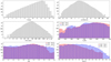 |
Fig. 1. Distribution in G, ϖ, distance (as derived by GSP-Phot Andrae et al. 2023), Teff, log g, and [M/H] for the sources for which the activity index has been derived. |
2.2. Reference inactive spectrum
We adopt a purely photospheric theoretical spectrum as reference inactive spectrum. The motivations and limitations of this choice are discussed extensively in Appendix B. Here we outline that this is a practical and robust assumption that allows us to put stars on a relative and homogeneous activity scale.
The purely photospheric theoretical spectrum is obtained by a linear interpolation over a grid of MARCS synthetic spectra at the stellar parameters (Teff, log g, [M/H]) as determined by GSP-Spec or GSP-Phot (Sect. 2.1). Linear interpolation is preferred to more elaborate spectrum representations because of the low computational cost combined with a reproduction of the observed spectrum which is satisfactory for our purposes (see e.g. Figs. 2 and 5). The synthetic spectra are computed under the assumption of local thermodynamic equilibrium (LTE) and radiative equilibrium (RE). As discussed in Appendix B, deviations from the LTE approximation are expected to be small in the range of parameters explored and not critical for our purposes. Also the assumption of RE does not pose critical issues in putting stars on a relative activity scale, despite the fact that the upper photosphere is not expected to be strictly in RE even in the most inactive stars. After interpolation, the reference spectrum is rotationally broadened at the projected rotational velocity vsini derived by the CU6 analysis (parameter vbroad). The interpolated rotationally broadened synthetic spectrum is taken as reference (or template) inactive spectrum.
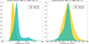 |
Fig. 2. Activity index histogram (bin size 0.001 nm, with KDE superimposed) normalised to peak values of stars with Teff ∈ (4000 K, 5000 K). Left panel: stars with log g > 4.0 (dwarfs) and right panel: stars with log g ∈ (3.0, 3.5). From this latter we estimate an upper limit to the true dispersion of the sample of 0.011 nm and 0.006 nm for the GSP-Spec and GSP-Phot input respectively, and an upper limit to the true bias of ≃0.002 nm (see text for details). |
2.3. Activity index
The activity index is derived by comparing the observed RVS spectrum with the RE model spectrum computed as described in the previous section. An excess equivalent width factor in the core of the Ca II IRT lines, computed on the observed-to-template ratio spectrum, is taken as an index of the stellar chromospheric activity or, in more extreme cases, of the mass accretion rate in PMS stars (see Appendix C). Given the template spectrum, the observed spectrum is first re-normalised by multiplying it by a third-order Chebyshev polynomial, whose coefficients are determined by minimising the pixel-to-pixel average deviation. The observed-to-template ratio spectrum is then calculated on a common wavelength grid at the stellar rest frame. The ratio spectrum is integrated on a ±Δλ = 0.15 nm interval around the core of each of the triplet lines and the mean of the three values obtained is taken as activity index. Formally, the activity index (α, parameter activityindex_espcs in nm units in the Gaia DR3 catalog) is defined as
 (1)
(1)
where  and
and  are the observed and the template spectrum, respectively, normalised to the continuum,
 (2)
(2)
Uncertainties (parameter activityindex_espcs_uncertainty in nm units in the Gaia DR3 catalog) are evaluated by propagating the pixel standard error, ignoring theoretical uncertainties.
The parameter α is close to zero for inactive stars and positive for active stars, with values above ≃0.03−0.05 nm indicating a possible contribution to the line flux due to mass accretion processes (Sect. 3.4) or enhanced activity in close binaries due to tidal interaction. Small negative values may derive from uncertainties in the input parameters or be physically plausible for low levels of chromospheric activity (see Appendix B).
The activity index α defined in Eq. (1) is suitable for comparing activity in stars with similar fundamental parameters (Teff, log g, [M/H]), but unsuitable for the comparison in stars with significantly different fundamental parameters, especially those with different Teff. In fact, a given value of α corresponds to significantly different values of the chromospheric flux contribution when the underlying continuum flux is significantly different. In order to overcome the difficulties posed by this ‘contrast’ effect, an index  , which is conceptually similar to
  , can be derived from α and the stellar parameters. First, we note that α is related to the excess equivalent width
 (3)
(3)
by the relation
 (4)
(4)
where ⟨rλ⟩core is the expected line-to-continuum average flux ratio in the core (±0.15 nm from central λ) of the Ca II IRT lines in radiative equilibrium. The activity flux ℱ′ at the stellar surface, being either chromospheric activity or accretion flux, can be obtained by the relation:
 (5)
(5)
where ℱc is the continuum flux at the stellar surface1. By analogy to  , the
, the  index can therefore be defined as
 (6)
(6)
which gives the flux difference with respect to the radiative equilibrium approximation in the core of the Ca II IRT lines in bolometric flux units and, for α > 0, is suitable for comparing the activity level over the whole range of parameters explored (see Appendix B).
The quantity in brackets in Eq. (6) depends mainly on Teff, it is weakly dependent on metallicity and has a negligible dependence on log g in the range of parameters explored in Gaia DR3. We approximated the log of this quantity with a third-order polynomial in θ = log Teff for four values of [M/H]. The fit coefficients are reported in Table 1. Using this polynomial fit,  can be estimated from α and Teff for a given [M/H] as:
 (7)
(7)

3. Scientific validation
ESP-CS has processed stars with G < 13, Teff in the range 3000 K–7000 K, log g in the 3.0–5.5 range, and [M/H] in the −1.0–1.0 range. The activity index α has been estimated on a total of approximately 2M stars; in DR3 α has a range ≈−0.1–1.0. As an example, Fig. 2 reports the activity index histogram for stars with Teff ∈ (4000 K, 5000 K). Negative values are physically expected because in low-activity stars the chromosphere causes a deeper line absorption than the radiative equilibrium expectation (see Appendix B); uncertainties in the astrophysical parameters can also cause negative values. Nominal uncertainties take the pixel noise into account and are ∼0.001 nm on average.
The activity index for the bulk of K stars with the lowest log g (3.0 ≤ log g ≤ 3.5) has a standard deviation of 0.011 and 0.006 nm in the case of GSP-Spec and GSP-Phot input, respectively (Fig. 2, right panel). As these stars –which exclude subgiants in close active binaries such as RS CVn systems– have the lowest activity in the parameter range explored, such standard deviations can be taken as upper limits of the random errors of the whole sample. The average activity index for these stars is 0.002 nm for both the GSP-Phot and GSP-Spec input; this can be considered an upper limit to the true bias.
Astrophysical parameters for rapidly rotating and emission-line stars are generally provided by GSP-Phot only. As these are also the most active stars, the distribution with GSP-Phot input is peaked and extended to larger values than the distribution of the activity index with GSP-Spec input.
3.1. Activity index versus Teff
Figure 3 shows the 2D density plot  versus Teff with input parameters from GSP-Phot and GSP-Spec separately. In the dataset with input parameters from GSP-Phot (Fig. 3, upper left panel), the high-activity part, for example for
  , is characterised by two almost horizontal branches, bending towards lower
  values at decreasing Teff below 4000 K and disappearing below 3500 K.
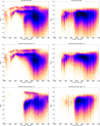 |
Fig. 3. Density plots of |

The clustering of  in these three different regimes is further outlined in the histogram shown in Fig. 4. The highest branch (very high activity, ‘VHA’ hereafter) has a lower limit of between
  and −5.0 depending on Teff. The second highest branch (high activity, HA hereafter) has a lower limit of between
  and −5.5 depending on Teff. The limit between the second highest branch and the bulk of low-activity (LA) stars is at
  .
.
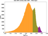 |
Fig. 4. Histogram of |

There is a clear gap between the HA branch and the LA branch starting at Teff ≃ 5400 K and  and growing at decreasing Teff until it disappears at Teff ≃ 4500 K (upper left panel of Fig. 3). However, this gap disappears when considering stars with log g > 4.0 only (Fig. 3, middle left panel). The comparison between the upper panels and the middle (log g > 4.0) and lower (log g < 4.0) panels of Fig. 3 reveals that the structure of LA stars bending down in this Teff range is in fact populated by more evolved stars, approximately in the subgiant branch of the Hertzsprung-Russell diagram (HRD), with a low level of chromospheric activity.
These results are consistent with what the finding of Henry et al. (1996) and Gomes da Silva et al. (2021), who suggested a grouping of very active stars with  (corresponding approximately to
  , according to the correlation discussed in Sect. 3.2) and very inactive stars with
  (corresponding approximately to
  ), with a regime of active stars in between these values.
The same density plot with input parameters from GSP-Spec (Fig. 3, upper right panel) does not show such clustering. This is likely due to the higher dispersion of  with input parameters from GSP-Spec (as suggested by a visual comparison between the two diagrams in Fig. 3 and supported by the comparison with
  in Sect. 3.2) and the lack of GSP-Spec parameters for active and fast-rotating stars that populate the higher part of the diagram (see Sects. 3.4 and 3.6). We note that the higher dispersion of
  with input from GSP-Spec suggested by Fig. 3 is consistent with the higher α dispersion found in stars with Teff ∈ (4000 K, 5000 K) and log g ∈ (3.0, 3.5) (see above and Fig. 2).
In Fig. 5 some Ca II IRT sample spectra of stars in the different regimes are shown: a subgiant and a dwarf in the LA regime, a dwarf in the HA regime and an accreting star (one in the Upper Scorpius association reported in Table 2 and Fig. 8) in the VHA regime. The spectra are compared with the template and the enhancement with respect to the template spectrum is shown.
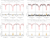 |
Fig. 5. Ca II IRT sample spectra in the different regimes. In each panel, the spectra (black line) are compared with the template (red line). The enhancement factor, i.e. the integrand of Eq. (1), is reported below the spectrum, and the integral producing α is outlined in orange. Upper left panel: LA subgiant with |
The activity distribution is found to be very different for Teff ≲ 3500 K, which corresponds to the transition between partially convective to fully convective stars. Figure 3 shows that stars close to the partially convective–fully convective boundary show a large drop in chromospheric activity, which increases again with decreasing Teff (mass) in the fully convective regime. A paucity of stars is found in the  diagram at 3300 K ≲ Teff ≲ 3500 K, which is likely related to the gap in the mid-M MS found by Jao et al. (2018), which itself has been linked to the onset of full convection in M dwarfs (Jao et al. 2018; Mayne 2010; MacDonald & Gizis 2018; Baraffe & Chabrier 2018).
3.2. Comparison with the  chromospheric activity index
In order to relate  with
with  , we estimated
  on ESO-FEROS archive spectra and further considered the data provided by Boro Saikia et al. (2018), which include a compilation of
  values from various surveys plus their own measurements on archive HARPS spectra. For simplicity, our approximate estimate of
  from FEROS spectra have been carried out as in Linsky et al. (1979), without considering more recent calibrations of the H & K surface flux (Middelkoop 1982; Rutten 1984) nor rescaling to the Mount Wilson data as in Boro Saikia et al. (2018).
Deriving an accurate  versus
  relationship would require a consistent estimate of the photospheric contribution and a homogenisation of the methods used in deriving
  , considering also the non-simultaneity of the measurements and the intrinsic variability of chromospheric activity. This is outside the scope of the present work and is left for future work, as is the publication of the
  values from archive FEROS spectra. Here we simply aim to verify the existence of the correlation between
  and
and  and at providing some preliminary approximate relationships between the two parameters.
A cross-match with the Gaia DR3 activity index leads to 671 objects in common with our  estimate from FEROS spectra (362 with GSP-Spec and 309 with GSP-Phot input parameters) and 220 objects in common with the Boro Saikia et al. (2018) dataset. As discussed above (see Figs. 2 and 4),
  with GSP-Spec input is characterised by a larger dispersion and is more concentrated on the lower activity range, while
  with GSP-Phot input has a lower dispersion and extends to a higher activity range. The cross-match with the FEROS data reflects this situation; in Fig. 7, which shows the
  versus
  dispersion diagram, data with GSP-Spec input cover mostly the lower left part while data with GSP-Phot input cover mostly the upper right part of the diagram. Data with GSP-Spec input are also affected by a larger dispersion than data with GSP-Phot input or the Boro Saikia et al. (2018) dataset.
The  with GSP-Phot input is well correlated with FEROS
  , with a Pearson linear correlation coefficient r = 0.74 and
 (8)
(8)
The  with GSP-Spec input is poorly correlated with FEROS
  , having r = 0.31; this is mainly due to the fact that the GSP-Spec APs in Gaia DR3 concern mostly stars with a low level of activity and therefore a regime in which the activity index signal-to-noise ratio is lower. The larger variance of α with GSP-Spec input with respect to the GSP-Phot input (see above and Fig. 2, right panel), could itself be due to the lower activity index signal-to-noise ratio in the regime covered by GSP-Spec, or to an intrinsically larger variance of the GSP-Spec APs. Despite such limitations, the activity index derived with GSP-Spec input APs maintains its validity of a relative chromospheric activity indicator in the LA regime.
The correlation with the Boro Saikia et al. (2018) dataset has r = 0.50 and
 (9)
(9)
3.3. Position in the colour–magnitude diagram
Consistency of the activity index scale is also verified by examining the position of the three branches in the Gaia CMD (MG vs. (GBP − GRP) corrected for interstellar extinction; Andrae et al. 2023). Figure 6 shows the position of subsamples of each branch superimposed on the CMD of all sources for which the activity index has been derived. The range of input APs considered implies that the CMD in Fig. 6 includes the lower MS, the subgiant branch and the PMS regions. The MS, in turn, is split into two sequences, with the over-density associated with the higher sequence notoriously due mainly to binary stars, but with PMS stars transiting over the same region while they contract towards the ZAMS. In the following, we refer to the single-star MS as the single-MS and to the binary star MS as binary-MS. In order to consider homogeneous results that include PMS and fast-rotating stars, only results with GSP-Phot input are shown.
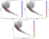 |
Fig. 6. Position in the CMD, corrected for interstellar extinction, of stars in the VHA (upper left panel), HA (upper right panel) and LA (lower panel) branches. Input APs are from GSP-Phot. The density plot of all sources for which the activity index has been derived is shown in grey on the background. The position of subsamples of ∼2000 stars per branch are shown in each panel, colour coded according to |

The first panel of Fig. 6 shows that stars in the VHA-branch ( ) are preferentially located above the single-MS, and the higher
  , the higher the tendency to be located at larger distance above the single-MS. However, we note, however, that some of the most active stars are located on or close to the single- and binary-star MS. Furthermore, some of the most active stars are early-K stars at ∼2−4 mag above the MS. The second panel of Fig. 6 shows that stars in the HA-branch (
 ) are mostly concentrated on the single-MS, with some stars on the binary-MS and a few above the MS. Contrary to the VHA stars location, the region of early-K stars at ∼2−4 mag above the MS, where we can find RS CVns and PMSs, is essentially void of HA stars. The third panel shows that stars in the LA-branch (
 ) are mostly concentrated in the F- G-type MS, with a few in the subgiant region. Consistently with the discussion in Sect. 3.1 (Fig. 3), the late-K, M star region is almost void of LA stars. LA stars populate the early-K region at ∼2−4 mag above the MS, with some of the least active stars concentrated here.
In support of the scientific validity of the results published in Gaia DR3, in the following sections we discuss the consistency with current knowledge of the distribution of the three branches in the CMD.
3.4. The very high activity branch
A cross-match of stars in the VHA-branch with the SIMBAD database shows that these objects are mostly classified as PMS stars, including Young Stellar Object (YSO), T Tau, and Orion-type variables. A few RS CVns are also present.
In PMS stars, mass accretion can cause an excess flux in the Ca II IRT lines that dominates over the chromospheric flux (see Appendix C). Figure 8 shows the comparison of  with mass accretion rate (log Ṁ) for 17 objects for which an estimate of the mass accretion rate is available. The log Ṁ estimates in Fig. 8 come from either the Hα width at 10% of the peak (Natta et al. 2004; Alcalá et al. 2014) measured by the Gaia-ESO survey (Lanzafame et al. 2015)2 or are derived from the excess continuum emission (see, e.g. Manara et al. 2015). The source identification, membership, and log Ṁ references are reported in Table 2. The
  versus log Ṁ correlation is weak in all cases, that is considering the whole set, the measurements based on Hα width at 10% of the peak or on the excess continuum (r ∼ 0.3). Nevertheless, all these objects have
  .
.
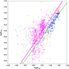 |
Fig. 7. Comparison of |


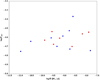 |
Fig. 8. Activity index ( |

Previous knowledge (e.g. Linsky 2017, and references therein) indicates that VHA stars on or close to the binary-MS can be identified as either chromospherically active dwarf stars in binary systems or PMS stars. Stars located above the binary-MS can also be identified as PMS/T Tauri stars at an earlier phase of contraction towards the ZAMS, or, when they are located in the subgiant region, as RS CVn systems in which at least one component is a subgiant. The distribution of VHA stars in the CMD (Fig. 6, upper panel) is consistent with this scenario, confirming the validity of the Gaia DR3 activity index. This situation also suggests that amongst stars in the very active branch ( ) there is a superposition of mass-accreting stars and stars with enhanced activity, as that induced by tidal interaction in close binary system like RS CVn. As a consequence, the separation between the very high activity branch and the high activity branch seen in the upper left panel of Fig. 3 can be due to the rapid decrease of mass accretion in PMS stars, but the very high activity branch is populated by both PMS accreting stars and other very active systems like RS CVn. The HA branch is therefore expected to be populated by chromospherically active stars with no mass accretion (see also Sect. 3.6). A dividing line between pure chromospheric activity and mass-accretion-dominated regimes can be placed at
  values of between approximately −4.8 and −5.0, depending on Teff (see also Fig. 4), but a value of
  above this limit may be due to enhanced activity in RS CVn systems as well.
3.5. The high- and low-activity branches: The Vaughan-Preston gap
Vaughan & Preston (1980) found a gap at some intermediate level of chromospheric activity in F and G stars observed in the Mount Wilson project. This gap has been thoroughly discussed in the literature with different interpretations (e.g. Durney et al. 1981; Noyes et al. 1984; Rutten 1987; Pace et al. 2009). Recently, Boro Saikia et al. (2018) investigated this issue using their extensive compilation of  , finding that for F, G, and early-K stars this gap is indeed particularly apparent. These authors instead found, instead, that moving towards late-K and early-M dwarfs, the concentration of stars on the active side of the gap increases and decreases on the low-activity side.
The plots in Fig. 3 confirm the findings of Boro Saikia et al. (2018). Considering only stars with log g > 4.0 and excluding the upper branch populated by PMS stars, we find no clear evidence of a gap at Teff corresponding to F, G, and early-K stars. The middle panels of Fig. 3, on the other hand, confirm the disappearance of low-activity stars at decreasing Teff. Below ≈4500 K, almost only the high-activity branch remains, which bends towards lower activity below ≈4000 K. Subsequently, below ≈3500 K, the spread in  increases dramatically and the branch is no longer distinguishable.
Indeed, the histogram in Fig. 4 does show a decrease in the number of stars at  , which would suggest a bimodal distribution in chromospheric activity with a clear minimum in between. However, the histograms shown in Fig. 9 show that the two peaks on both sides of this minimum are mostly due to the combination of the different
  distributions for stars cooler and hotter than Teff ≈ 5000 K. Restricting the sample to stars with log g > 4.0 and not considering stars in the highest activity branch populated by PMS stars, the distribution of stars with Teff ≳ 5000 K peaks at
  and has only a bump at
  , showing only a shallow minimum in between, which remains so even when further restricting the bin size. On the other hand, the distribution of dwarfs with Teff ≲ 5000 K peaks at
  and shows no bump on either side of the maximum. The cumulative distribution, which gathers together the different behaviours on either side of the Teff ≈ 5000 K boundary, shows a double peak with a clear minimum at
  .
.
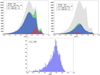 |
Fig. 9.
|

All stars with log g < 4.0 (Fig. 9, right panel) below  have a unimodal distribution, those with Teff < 5000 K peaking at
  and those with Teff < 5000 K peaking at
  . The distribution of stars with log g < 4.0 also has a secondary peak above
  , which may be associated with subgiants in close binaries with enhanced activity.
In summary, only dwarfs with Teff ≳ 5000 K show a hint of a bimodal distribution, with central values at  and −5.20, but without a clear gap in between. Notably, according to Eqs. (8) and (9), the Vaughan-Preston gap at
  corresponds to
  , which places it in between the estimated central values of the HA and LA branches.
3.6. Comparison with rotational modulation
The DPAC analysis includes the detection and characterisation of rotational modulation due to photospheric active regions (variability coordination unit, CU7, Lanzafame et al. 2018). Gaia DR3 included rotational modulation data for some 150 000 stars (Lanzafame et al. 2018) and Gaia DR3 includes data for some 500 000 stars (Distefano et al. 2023).
Lanzafame et al. (2019) found that the rotational modulation amplitude distribution in Gaia DR3 data shows a clear bimodality, with an evident gap at an amplitude of A ≃ 0.04 − 0.05 mag. The low-amplitude branch in turn shows a period bimodality with a main clustering at periods P ≈ 5 − 10 d and a secondary clustering of ultra-fast rotators at P ≲ 0.5 d. These three different branches in the period–amplitude diagram were named high-amplitude rotators (HARs), low-amplitude fast-rotators (LAFRs), and low-amplitude slow-rotators (LASRs). Lanzafame et al. (2019) interpreted these branches as signatures of different surface inhomogeneity regimes and suggested possible scenarios for their evolution. The amplitude–period multimodality was found to be correlated with the position in the period–absolute magnitude (or period–color) diagram, with the low- and high-amplitude stars occupying different preferential locations.
Figure 10 shows the positions of stars with different rotation modulation amplitude A in the  versus Teff density diagram. A clear correlation between
  and A is found (r ≈ 0.6), as expected (see e.g. Linsky 2017, and references therein), which increases when considered on a Teff by Teff basis (r ≈ 0.7). Confirmation of the consistency between rotational modulation and the activity index data in Gaia DR3 also comes from the comparison with the branches identified in Lanzafame et al. (2019). Stars in the HAR-branch of the period–amplitude diagram are found to be located in the VHA-branch of the
  versus Teff density diagram. We note that the HAR-branch is populated mainly by PMS stars (Lanzafame et al. 2019) as is the VHA-branch (see Sect. 3.4). Stars in the LASR-branch of the period–amplitude diagram are found in the HA and LA branches of the
  versus Teff density diagram, with the highest A in this range mostly located in the HA branch.
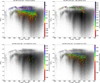 |
Fig. 10.
|

The position in the  versus Teff density diagram of the few LAFR stars in common is of particular interest. Lanzafame et al. (2019) suggested that the small modulation amplitude of stars in the LAFR branch may be due to a high degree of axisymmetry of the surface magnetic field. If this were the main difference compared to the HAR branch, one could naively expect the chromospheric activity in the LAFR and HAR branches to be relatively similar. The bottom left panel of Fig. 10 instead suggests a more complex scenario. Most of the LAFR with Teff ≲ 5000 K are placed on the HA branch, the lowest available in this Teff range, with only one star on the VHA branch. LAFR stars with Teff ≳ 5000 K are mostly in the LA branch, with a few on the HA branch and only one in the VHA branch. In general, there is no clear evidence of a correlation between chromospheric and photospheric activity in LAFR stars, but both are, unlike HAR stars, at low level. This suggests that a high degree of axisymmetry of the surface magnetic field may not be the only cause of the low rotational modulation amplitude in these stars, but rather that magnetic activity is inhibited in LAFR stars with respect to HAR stars with similar rotation period. It may be argued that the LAFR sample may be contaminated by stars above the Kraft limit –that is, stars with a radiative core and a convective envelope– because of an incorrect estimate of both interstellar extinction and Teff. The variability in this case could be due to stellar pulsation rather than rotational modulation. Although we cannot exclude the presence of contaminants in the LAFR sample, there is evidence that at least a good fraction of them are real low-mass stars. In fact, about 50 of them have APs in very good agreement between GSP-Phot and GSP-Spec, this latter being unaffected by interstellar absorption. Furthermore, from the distances of the stars we estimate that for at least 50% of them the interstellar extinction estimate by GSP-Phot should be biased by more than 3 mag kpc−1 to be high-mass stars that appear as low-mass stars, which is deemed quite unlikely.
4. Conclusions
Gaia DR3 contains the largest chromospheric activity index catalogue obtained to date. The activity index was derived from the Ca II IRT observed by the Gaia Radial Velocity Spectrometer (RVS) for 2 141 643 stars in the Galaxy, with G < 13, Teff ∈ (3000 K, 7000 K), log g ∈ (3.0, 5.5), and [M/H] ∈ (−1.0, 1.0). In this paper, we describe the method used and the results from the scientific validation. We also provide a simple formula (Eq. (7)) to convert the parameter published in the catalogue (activityindex_espcs) to the  index, which is analogous to the
  index derived from the Ca II H & K doublet and is suitable for comparing the activity level over the whole range of parameters explored in Gaia DR3.
The scientific validation of the activity index obtained using the GSP-Phot parameters as input confirms the existence of three different regimes, which we call very high activity (VHA,  ), high activity (HA,
  ), and low activity (LA,
  ). The activity index obtained using the GSP-Spec parameters as input does not show such clustering because of an evidently larger dispersion with respect to the results obtained with the GSP-Phot input and the GSP-Spec filtering applied to the most active stars like fast-rotator and PMS. The activity regimes found with the GSP-Phot input are consistent with those suggested by Henry et al. (1996) and confirmed recently by Gomes da Silva et al. (2021) from the analysis of
  .
.
The VHA regime is found to be populated by PMS stars and close binary system like RS CVns. In the former, the excess flux with respect to the radiative equilibrium condition may be dominated by mass accretion. In the latter, magnetic activity may be significantly enhanced by tidal interaction. A comparison between  and mass accretion rate Ṁ for a few PMS stars in the sample (Fig. 8) shows that, although the two parameters are not clearly correlated, a value
  may indicate a significant mass accretion flux contribution to the emission core of Ca II IRT. Indeed, the gap between the VHA branch and the rest of the distribution in the
  versus Teff diagram (Fig. 3) can be due to the rapid transition from the regime dominated by mass accretion to the regime dominated by magneto-acoustic heating of the chromosphere.
The  distribution (Fig. 9) is found to depend on Teff and log g. Stars with Teff < 5000 K and log g > 4.0 are in the HA and VHA branches. Excluding the VHA, the distribution of these stars in the HA branch is unimodal, peaking at
  . The distribution of stars with Teff ≳ 5000 K and log g > 4.0, on the other hand, peaks at
  and has a bump at
  , with a shallow minimum in between. This minimum corresponds approximately to the location of the Vaughan-Preston gap at
  (Vaughan & Preston 1980), but this range is far from being void of stars, confirming the findings of Boro Saikia et al. (2018). Stars with Teff ≳ 5000 K and log g > 4.0 are therefore found in all three regimes, while stars with Teff < 5000 K and log g > 4.0 are found in the VHA and HA regimes only.
Stars with log g ∈ (3.0,4.0) have unimodal distributions in the LA regime, peaking at  for Teff < 5000 K, and at
  for Teff ≳ 5000 K. There are also a few stars in the VHA regime that are likely to be subgiants in close binaries with enhanced activity.
The activity distribution is found to change dramatically in the fully convective regime (Fig. 3). Stars close to the partially convective–fully convective boundary show a large drop in chromospheric activity; then, at decreasing Teff (mass), activity increases again to reach approximately the same level of partially convective stars in the HA branch. A paucity of stars is found in the  diagram at 3300 K ≲ Teff ≲ 3500 K, which is likely connected to the gap in the mid-M dwarfs MS found by Jao et al. (2018) linked to the onset of full convection in M dwarfs.
The  index derived from the Gaia DR3 activity index is well correlated with
  from Boro Saikia et al. (2018), who gathered together a compilation of values from various surveys plus their own measurements on archive HARPS spectra. We also find good correlation with a preliminary
  estimate made on ESO-FEROS archive spectra, which will be the subject of future work.
The correlation of  with the position in the Gaia CMD (Fig. 6) is in line with the current knowledge of the activity evolution of low-mass stars (see e.g. Linsky 2017). Stars in the VHA branch, which according to a cross-match with the SIMBAD database includes PMS stars and RS CVn systems, are preferentially located above the single-star MS, the higher
  the higher the tendency to be located at larger distance above the MS. A group of very active early-K stars is found at ∼2−4 mag above the MS. Some very active stars are also located close to the single- and binary-star MS. Stars in the HA branch tend to be on the single-star MS, with some stars on the binary-MS and a few above the MS. The region of early-K stars at ∼2−4 mag above the MS is essentially void of HA stars. Finally, stars in the LA branch are mostly concentrated in the F- G-type MS and in the subgiant region, with the early-K region at ∼2−4 mag above the MS populated with some of the most inactive stars. In this latter region, we therefore have a superposition of VHA (close binaries or PMS stars) and LA stars (very inactive subgiants).
The  diagram has a neat and unambiguous correspondence with the period–amplitude diagram (PAD) of the rotational modulation due to photospheric spot and faculae (Lanzafame et al. 2018, 2019; Distefano et al. 2023). Stars in the high amplitude rotator branch (HAR) of the PAD, as identified for the first time by Lanzafame et al. (2019) in the Gaia DR3 data, have a clear correspondence with the VHA branch in the
  diagram. Both are populated by young, PMS stars. The low-amplitude slow-rotator branch (LASR) of the PAD corresponds to the HA and LA branches of the
  diagram.
The position of the low-amplitude fast-rotator (LAFR) stars in the  diagram is particularly interesting. Despite the high rotation velocity, these stars have low rotational modulation amplitude and most of them also have low chromospheric activity index. The former may be due either to a small photospheric active region filling factor or to a high degree of axisymmetry of the surface magnetic field. The latter can only be due to a global low level of magneto-acoustic heating of the chromosphere, with the axisymmetry of the surface magnetic field expected to play almost no role. The evidence points therefore to a global low level of photospheric and chromospheric activity rather than to a high degree of axisymmetry of the surface magnetic field in these fast rotating stars. Moreover, Distefano et al. (2023), who presented the rotational modulation data in Gaia DR3, find a low correlation between the G variation due to rotational modulation and the (GBP − GRP) colour variation in LAFR stars, which, combined with the low rotational modulation amplitude and the small chromospheric activity index, strengthen the evidence of the presence of smaller active regions in this branch compared with stars in the HAR branch with similar rotation period. In general, there is a good correlation between the chromospheric activity index and the amplitude of the rotational modulation due to spot and faculae, which is tighter when examined on limited colour or Teff bins.
Overall, the scientific validation of the Gaia DR3 stellar activity index derived from the analysis of the Ca II IRT observed by RVS demonstrates a high level of consistency with previous results, most of them obtained from the analysis of the Ca II H & K doublet, extending these results to a much larger sample. The richness of the Gaia sample allows us to derive the distribution of the stellar activity over stellar fundamental parameters with an unprecedented level of detail, outlining different regimes of chromospheric heating and identifying those where the emission due to mass-accretion processes may dominate over a purely chromospheric emission. The activity index provided in Gaia DR3 therefore represents a ‘gold mine’ for several investigations, such as: verifying or falsifying theoretical models of the stellar dynamo and of the emergence of stellar active regions; identifying stars with a low RV jitter in the search for Earth-like planets; studying the impact of magnetic activity in the derivation of accurate elemental abundance in stellar atmospheres; studying the evolution of the magnetic activity for different stellar mass and its impact on the host exoplanets; and studying the magnetic activity in close binary systems.
We note that by expressing ℱc in [W m−2 nm−1], ℱ′ has units [W m−2], expressing the chromospheric contribution to the flux in the line integrated over a wavelength range around the core of the line.
Data available at https://www.eso.org/qi/catalogQuery/index/121
Acknowledgments
The full acknowledgements are available in Appendix A.
References
- Airapetian, V. S., Barnes, R., Cohen, O., et al. 2020, Int. J. Astrobiol., 19, 136 [NASA ADS] [CrossRef] [Google Scholar]
- Alcalá, J. M., Natta, A., Manara, C. F., et al. 2014, A&A, 561, A2 [NASA ADS] [CrossRef] [EDP Sciences] [Google Scholar]
- Amard, L., Roquette, J., & Matt, S. P. 2020, MNRAS, 499, 3481 [NASA ADS] [CrossRef] [Google Scholar]
- Andrae, R., Fouesneau, M., Sordo, R., et al. 2023, A&A, 674, A27 ({\it Gaia} DR3 SI) [NASA ADS] [CrossRef] [EDP Sciences] [Google Scholar]
- Andretta, V., Busà, I., Gomez, M. T., & Terranegra, L. 2005, A&A, 430, 669 [NASA ADS] [CrossRef] [EDP Sciences] [Google Scholar]
- Bailer-Jones, C. A. L. 2011, MNRAS, 411, 435 [Google Scholar]
- Bailer-Jones, C. A. L., Andrae, R., Arcay, B., et al. 2013, A&A, 559, A74 [NASA ADS] [CrossRef] [EDP Sciences] [Google Scholar]
- Baraffe, I., & Chabrier, G. 2018, A&A, 619, A177 [NASA ADS] [CrossRef] [EDP Sciences] [Google Scholar]
- Barnes, S. A. 2003, ApJ, 586, 464 [Google Scholar]
- Barnes, S. A. 2007, ApJ, 669, 1167 [Google Scholar]
- Barnes, S. A. 2010, ApJ, 722, 222 [Google Scholar]
- Barrado y Navascués, D., & Martín, E. L. 2003, AJ, 126, 2997 [Google Scholar]
- Bastien, F. A., Stassun, K. G., Pepper, J., et al. 2014, AJ, 147, 29 [Google Scholar]
- Batalha, C. C., Stout-Batalha, N. M., Basri, G., & Terra, M. A. O. 1996, ApJS, 103, 211 [NASA ADS] [CrossRef] [Google Scholar]
- Boro Saikia, S., Marvin, C. J., Jeffers, S. V., et al. 2018, A&A, 616, A108 [NASA ADS] [CrossRef] [EDP Sciences] [Google Scholar]
- Busà, I., Aznar Cuadrado, R., Terranegra, L., Andretta, V., & Gomez, M. T. 2007, A&A, 466, 1089 [NASA ADS] [CrossRef] [EDP Sciences] [Google Scholar]
- Calvet, N., & Gullbring, E. 1998, ApJ, 509, 802 [Google Scholar]
- Campbell, B., Walker, G. A. H., & Yang, S. 1988, ApJ, 331, 902 [NASA ADS] [CrossRef] [Google Scholar]
- Carlsson, M., De Pontieu, B., & Hansteen, V. H. 2019, ARA&A, 57, 189 [Google Scholar]
- Cram, L. E., & Mullan, D. J. 1979, ApJ, 234, 579 [NASA ADS] [CrossRef] [Google Scholar]
- Creevey, O. L., Sordo, R., Pailler, F., et al. 2023, A&A, 674, A26 ({\it Gaia} DR3 SI) [NASA ADS] [CrossRef] [EDP Sciences] [Google Scholar]
- Distefano, E., Lanzafame, A. C., Brugaletta, E., et al. 2023, A&A, 674, A20 ({\it Gaia} DR3 SI) [NASA ADS] [CrossRef] [EDP Sciences] [Google Scholar]
- Duncan, D. K., Vaughan, A. H., Wilson, O. C., et al. 1991, ApJS, 76, 383 [Google Scholar]
- Durney, B. R., Mihalas, D., & Robinson, R. D. 1981, PASP, 93, 537 [NASA ADS] [CrossRef] [Google Scholar]
- Flores, M., González, J. F., Jaque Arancibia, M., Buccino, A., & Saffe, C. 2016, A&A, 589, A135 [NASA ADS] [CrossRef] [EDP Sciences] [Google Scholar]
- Fouesneau, M., Frémat, Y., Andrae, R., et al. 2023, A&A, 674, A28 ({\it Gaia} DR3 SI) [NASA ADS] [CrossRef] [EDP Sciences] [Google Scholar]
- Frasca, A., & Catalano, S. 1994, A&A, 284, 883 [NASA ADS] [Google Scholar]
- Frasca, A., Biazzo, K., Lanzafame, A. C., et al. 2015, A&A, 575, A4 [NASA ADS] [CrossRef] [EDP Sciences] [Google Scholar]
- Gaia Collaboration (Prusti, T., et al.) 2016, A&A, 595, A1 [NASA ADS] [CrossRef] [EDP Sciences] [Google Scholar]
- Gaia Collaboration (Vallenari, A., et al.) 2023, A&A, 674, A1 ({\it Gaia} DR3 SI) [NASA ADS] [CrossRef] [EDP Sciences] [Google Scholar]
- Gallet, F., & Bouvier, J. 2013, A&A, 556, A36 [NASA ADS] [CrossRef] [EDP Sciences] [Google Scholar]
- Gallet, F., & Bouvier, J. 2015, A&A, 577, A98 [NASA ADS] [CrossRef] [EDP Sciences] [Google Scholar]
- Gomes da Silva, J., Santos, N. C., Adibekyan, V., et al. 2021, A&A, 646, A77 [NASA ADS] [CrossRef] [EDP Sciences] [Google Scholar]
- Guilluy, G., Andretta, V., Borsa, F., et al. 2020, A&A, 639, A49 [EDP Sciences] [Google Scholar]
- Hartmann, L., Herczeg, G., & Calvet, N. 2016, ARA&A, 54, 135 [Google Scholar]
- Henry, T. J., Soderblom, D. R., Donahue, R. A., & Baliunas, S. L. 1996, AJ, 111, 439 [Google Scholar]
- Herbig, G. H. 1985, ApJ, 289, 269 [NASA ADS] [CrossRef] [Google Scholar]
- Ingleby, L., Calvet, N., Bergin, E., et al. 2011, ApJ, 743, 105 [CrossRef] [Google Scholar]
- Jao, W.-C., Henry, T. J., Gies, D. R., & Hambly, N. C. 2018, ApJ, 861, L11 [NASA ADS] [CrossRef] [Google Scholar]
- Kawaler, S. D. 1988, ApJ, 333, 236 [Google Scholar]
- Lanzafame, A. C., & Spada, F. 2015, A&A, 584, A30 [NASA ADS] [CrossRef] [EDP Sciences] [Google Scholar]
- Lanzafame, A. C., Frasca, A., Damiani, F., et al. 2015, A&A, 576, A80 [NASA ADS] [CrossRef] [EDP Sciences] [Google Scholar]
- Lanzafame, A. C., Distefano, E., Messina, S., et al. 2018, A&A, 616, A16 [NASA ADS] [CrossRef] [EDP Sciences] [Google Scholar]
- Lanzafame, A. C., Distefano, E., Barnes, S. A., & Spada, F. 2019, ApJ, 877, 157 [NASA ADS] [CrossRef] [Google Scholar]
- Linsky, J. L. 2017, ARA&A, 55, 159 [Google Scholar]
- Linsky, J. L., Worden, S. P., McClintock, W., & Robertson, R. M. 1979, ApJS, 41, 47 [NASA ADS] [CrossRef] [Google Scholar]
- Liu, C., Bailer-Jones, C. A. L., Sordo, R., et al. 2012, MNRAS, 426, 2463 [NASA ADS] [CrossRef] [Google Scholar]
- Luhn, J. K., Wright, J. T., Howard, A. W., & Isaacson, H. 2020, AJ, 159, 235 [Google Scholar]
- MacDonald, J., & Gizis, J. 2018, MNRAS, 480, 1711 [NASA ADS] [CrossRef] [Google Scholar]
- Mamajek, E. E., & Hillenbrand, L. A. 2008, ApJ, 687, 1264 [Google Scholar]
- Manara, C. F., Testi, L., Natta, A., & Alcalá, J. M. 2015, A&A, 579, A66 [NASA ADS] [CrossRef] [EDP Sciences] [Google Scholar]
- Manara, C. F., Natta, A., Rosotti, G. P., et al. 2020, A&A, 639, A58 [NASA ADS] [CrossRef] [EDP Sciences] [Google Scholar]
- Matt, S. P., MacGregor, K. B., Pinsonneault, M. H., & Greene, T. P. 2012, ApJ, 754, L26 [Google Scholar]
- Matt, S. P., Brun, A. S., Baraffe, I., Bouvier, J., & Chabrier, G. 2015, ApJ, 799, L23 [Google Scholar]
- Mayne, N. J. 2010, MNRAS, 408, 1409 [NASA ADS] [CrossRef] [Google Scholar]
- Middelkoop, F. 1982, A&A, 113, 1 [NASA ADS] [Google Scholar]
- Muzerolle, J., Hartmann, L., & Calvet, N. 1998, AJ, 116, 455 [Google Scholar]
- Muzerolle, J., Calvet, N., & Hartmann, L. 2001, ApJ, 550, 944 [Google Scholar]
- Natta, A., Testi, L., Muzerolle, J., et al. 2004, A&A, 424, 603 [NASA ADS] [CrossRef] [EDP Sciences] [Google Scholar]
- Noyes, R. W., Hartmann, L. W., Baliunas, S. L., Duncan, D. K., & Vaughan, A. H. 1984, ApJ, 279, 763 [Google Scholar]
- Pace, G., Melendez, J., Pasquini, L., et al. 2009, A&A, 499, L9 [NASA ADS] [CrossRef] [EDP Sciences] [Google Scholar]
- Recio-Blanco, A., de Laverny, P., Palicio, P. A., et al. 2023, A&A, 674, A29 ({\it Gaia} DR3 SI) [NASA ADS] [CrossRef] [EDP Sciences] [Google Scholar]
- Rutten, R. G. M. 1984, A&A, 130, 353 [NASA ADS] [Google Scholar]
- Rutten, R. G. M. 1987, A&A, 177, 131 [NASA ADS] [Google Scholar]
- Saar, S. H., Butler, R. P., & Marcy, G. W. 1998, ApJ, 498, L153 [NASA ADS] [CrossRef] [Google Scholar]
- Santos, N. C., Mayor, M., Naef, D., et al. 2000, A&A, 361, 265 [NASA ADS] [Google Scholar]
- Schrijver, C. J., Cote, J., Zwaan, C., & Saar, S. H. 1989, ApJ, 337, 964 [NASA ADS] [CrossRef] [Google Scholar]
- Skumanich, A. 1972, ApJ, 171, 565 [Google Scholar]
- Spada, F., & Lanzafame, A. C. 2020, A&A, 636, A76 [NASA ADS] [CrossRef] [EDP Sciences] [Google Scholar]
- Spina, L., Nordlander, T., Casey, A. R., et al. 2020, ApJ, 895, 52 [Google Scholar]
- Taylor, M. B. 2005, in Astronomical Data Analysis Software and Systems XIV, eds. P. Shopbell, M. Britton, & R. Ebert, ASP Conf. Ser., 347, 29 [Google Scholar]
- van Leeuwen, F., de Bruijne, J., Babusiaux, C., et al. 2022, Gaia DR3 Documentation, European Space Agency; Gaia Data Processing and Analysis Consortium, Online at https://gea.esac.esa.int/archive/documentation/GDR3/index.html [Google Scholar]
- van Saders, J. L., Ceillier, T., Metcalfe, T. S., et al. 2016, Nature, 529, 181 [Google Scholar]
- Vaughan, A. H., & Preston, G. W. 1980, PASP, 92, 385 [Google Scholar]
- Vaughan, A. H., Preston, G. W., & Wilson, O. C. 1978, PASP, 90, 267 [Google Scholar]
- Venuti, L., Stelzer, B., Alcalá, J. M., et al. 2019, A&A, 632, A46 [NASA ADS] [CrossRef] [EDP Sciences] [Google Scholar]
- Weber, E. J., & Davis, L., Jr. 1967, ApJ, 148, 217 [Google Scholar]
- Wright, J. T. 2005, PASP, 117, 657 [Google Scholar]
- Yana Galarza, J., Meléndez, J., Lorenzo-Oliveira, D., et al. 2019, MNRAS, 490, L86 [Google Scholar]
- Žerjal, M., Zwitter, T., Matijevič, G., et al. 2017, ApJ, 835, 61 [CrossRef] [Google Scholar]
Appendix A: Acknowledgements
This work presents results from the European Space Agency (ESA) space mission Gaia. Gaia data are processed by the Gaia Data Processing and Analysis Consortium (DPAC). Funding for the DPAC is provided by national institutions, in particular the institutions participating in the Gaia MultiLateral Agreement (MLA). The Gaia mission website is https://www.cosmos.esa.int/gaia. The Gaia archive website is https://archives.esac.esa.int/gaia.
The Gaia mission and data processing have financially been supported by, in alphabetical order by country:
-
the Algerian Centre de Recherche en Astronomie, Astrophysique et Géophysique of Bouzareah Observatory;
-
the Austrian Fonds zur Förderung der wissenschaftlichen Forschung (FWF) Hertha Firnberg Programme through grants T359, P20046, and P23737;
-
the BELgian federal Science Policy Office (BELSPO) through various PROgramme de Développement d’Expériences scientifiques (PRODEX) grants and the Polish Academy of Sciences – Fonds Wetenschappelijk Onderzoek through grant VS.091.16N, and the Fonds de la Recherche Scientifique (FNRS), and the Research Council of Katholieke Universiteit (KU) Leuven through grant C16/18/005 (Pushing AsteRoseismology to the next level with TESS, GaiA, and the Sloan DIgital Sky SurvEy – PARADISE);
-
the Brazil-France exchange programmes Fundação de Amparo à Pesquisa do Estado de São Paulo (FAPESP) and Coordenação de Aperfeicoamento de Pessoal de Nível Superior (CAPES) – Comité Français d’Evaluation de la Coopération Universitaire et Scientifique avec le Brésil (COFECUB);
-
the Chilean Agencia Nacional de Investigación y Desarrollo (ANID) through Fondo Nacional de Desarrollo Científico y Tecnológico (FONDECYT) Regular Project 1210992 (L. Chemin);
-
the National Natural Science Foundation of China (NSFC) through grants 11573054, 11703065, and 12173069, the China Scholarship Council through grant 201806040200, and the Natural Science Foundation of Shanghai through grant 21ZR1474100;
-
the Tenure Track Pilot Programme of the Croatian Science Foundation and the École Polytechnique Fédérale de Lausanne and the project TTP-2018-07-1171 ‘Mining the Variable Sky’, with the funds of the Croatian-Swiss Research Programme;
-
the Czech-Republic Ministry of Education, Youth, and Sports through grant LG 15010 and INTER-EXCELLENCE grant LTAUSA18093, and the Czech Space Office through ESA PECS contract 98058;
-
the Danish Ministry of Science;
-
the Estonian Ministry of Education and Research through grant IUT40-1;
-
the European Commission’s Sixth Framework Programme through the European Leadership in Space Astrometry (https://www.cosmos.esa.int/web/gaia/elsa-rtn-programme) Marie Curie Research Training Network (MRTN-CT-2006-033481), through Marie Curie project PIOF-GA-2009-255267 (Space AsteroSeismology & RR Lyrae stars, SAS-RRL), and through a Marie Curie Transfer-of-Knowledge (ToK) fellowship (MTKD-CT-2004-014188); the European Commission’s Seventh Framework Programme through grant FP7-606740 (FP7-SPACE-2013-1) for the Gaia European Network for Improved data User Services (https://gaia.ub.edu/twiki/do/view/GENIUS/) and through grant 264895 for the Gaia Research for European Astronomy Training (https://www.cosmos.esa.int/web/gaia/great-programme) network;
-
the European Cooperation in Science and Technology (COST) through COST Action CA18104 ‘Revealing the Milky Way with Gaia (MW-Gaia)’;
-
the European Research Council (ERC) through grants 320360, 647208, and 834148 and through the European Union’s Horizon 2020 research and innovation and excellent science programmes through Marie Skłodowska-Curie grant 745617 (Our Galaxy at full HD – Gal-HD) and 895174 (The build-up and fate of self-gravitating systems in the Universe) as well as grants 687378 (Small Bodies: Near and Far), 682115 (Using the Magellanic Clouds to Understand the Interaction of Galaxies), 695099 (A sub-percent distance scale from binaries and Cepheids – CepBin), 716155 (Structured ACCREtion Disks – SACCRED), 951549 (Sub-percent calibration of the extragalactic distance scale in the era of big surveys – UniverScale), and 101004214 (Innovative Scientific Data Exploration and Exploitation Applications for Space Sciences – EXPLORE);
-
the European Science Foundation (ESF), in the framework of the Gaia Research for European Astronomy Training Research Network Programme (https://www.cosmos.esa.int/web/gaia/great-programme);
-
the European Space Agency (ESA) in the framework of the Gaia project, through the Plan for European Cooperating States (PECS) programme through contracts C98090 and 4000106398/12/NL/KML for Hungary, through contract 4000115263/15/NL/IB for Germany, and through PROgramme de Développement d’Expériences scientifiques (PRODEX) grant 4000127986 for Slovenia;
-
the Academy of Finland through grants 299543, 307157, 325805, 328654, 336546, and 345115 and the Magnus Ehrnrooth Foundation;
-
the French Centre National d’Études Spatiales (CNES), the Agence Nationale de la Recherche (ANR) through grant ANR-10-IDEX-0001-02 for the ‘Investissements d’avenir’ programme, through grant ANR-15-CE31-0007 for project ‘Modelling the Milky Way in the Gaia era’ (MOD4Gaia), through grant ANR-14-CE33-0014-01 for project ‘The Milky Way disc formation in the Gaia era’ (ARCHEOGAL), through grant ANR-15-CE31-0012-01 for project ‘Unlocking the potential of Cepheids as primary distance calibrators’ (UnlockCepheids), through grant ANR-19-CE31-0017 for project ‘Secular evolution of galxies’ (SEGAL), and through grant ANR-18-CE31-0006 for project ‘Galactic Dark Matter’ (GaDaMa), the Centre National de la Recherche Scientifique (CNRS) and its SNO Gaia of the Institut des Sciences de l’Univers (INSU), its Programmes Nationaux: Cosmologie et Galaxies (PNCG), Gravitation Références Astronomie Métrologie (PNGRAM), Planétologie (PNP), Physique et Chimie du Milieu Interstellaire (PCMI), and Physique Stellaire (PNPS), the ‘Action Fédératrice Gaia’ of the Observatoire de Paris, the Région de Franche-Comté, the Institut National Polytechnique (INP) and the Institut National de Physique nucléaire et de Physique des Particules (IN2P3) co-funded by CNES;
-
the German Aerospace Agency (Deutsches Zentrum für Luft- und Raumfahrt e.V., DLR) through grants 50QG0501, 50QG0601, 50QG0602, 50QG0701, 50QG0901, 50QG1001, 50QG1101, 50QG1401, 50QG1402, 50QG1403, 50QG1404, 50QG1904, 50QG2101, 50QG2102, and 50QG2202, and the Centre for Information Services and High Performance Computing (ZIH) at the Technische Universität Dresden for generous allocations of computer time;
-
the Hungarian Academy of Sciences through the Lendület Programme grants LP2014-17 and LP2018-7 and the Hungarian National Research, Development, and Innovation Office (NKFIH) through grant KKP-137523 (‘SeismoLab’);
-
the Science Foundation Ireland (SFI) through a Royal Society – SFI University Research Fellowship (M. Fraser);
-
the Israel Ministry of Science and Technology through grant 3-18143 and the Tel Aviv University Center for Artificial Intelligence and Data Science (TAD) through a grant;
-
the Agenzia Spaziale Italiana (ASI) through contracts I/037/08/0, I/058/10/0, 2014-025-R.0, 2014-025-R.1.2015, and 2018-24-HH.0 to the Italian Istituto Nazionale di Astrofisica (INAF), contract 2014-049-R.0/1/2 to INAF for the Space Science Data Centre (SSDC, formerly known as the ASI Science Data Center, ASDC), contracts I/008/10/0, 2013/030/I.0, 2013-030-I.0.1-2015, and 2016-17-I.0 to the Aerospace Logistics Technology Engineering Company (ALTEC S.p.A.), INAF, and the Italian Ministry of Education, University, and Research (Ministero dell’Istruzione, dell’Università e della Ricerca) through the Premiale project ‘MIning The Cosmos Big Data and Innovative Italian Technology for Frontier Astrophysics and Cosmology’ (MITiC);
-
the Netherlands Organisation for Scientific Research (NWO) through grant NWO-M-614.061.414, through a VICI grant (A. Helmi), and through a Spinoza prize (A. Helmi), and the Netherlands Research School for Astronomy (NOVA);
-
the Polish National Science Centre through HARMONIA grant 2018/30/M/ST9/00311 and DAINA grant 2017/27/L/ST9/03221 and the Ministry of Science and Higher Education (MNiSW) through grant DIR/WK/2018/12;
-
the Portuguese Fundação para a Ciência e a Tecnologia (FCT) through national funds, grants SFRH/-BD/128840/2017 and PTDC/FIS-AST/30389/2017, and work contract DL 57/2016/CP1364/CT0006, the Fundo Europeu de Desenvolvimento Regional (FEDER) through grant POCI-01-0145-FEDER-030389 and its Programa Operacional Competitividade e Internacionalização (COMPETE2020) through grants UIDB/04434/2020 and UIDP/04434/2020, and the Strategic Programme UIDB/-00099/2020 for the Centro de Astrofísica e Gravitação (CENTRA);
-
the Slovenian Research Agency through grant P1-0188;
-
the Spanish Ministry of Economy (MINECO/FEDER, UE), the Spanish Ministry of Science and Innovation (MICIN), the Spanish Ministry of Education, Culture, and Sports, and the Spanish Government through grants BES-2016-078499, BES-2017-083126, BES-C-2017-0085, ESP2016-80079-C2-1-R, ESP2016-80079-C2-2-R, FPU16/03827, PDC2021-121059-C22, RTI2018-095076-B-C22, and TIN2015-65316-P (‘Computación de Altas Prestaciones VII’), the Juan de la Cierva Incorporación Programme (FJCI-2015-2671 and IJC2019-04862-I for F. Anders), the Severo Ochoa Centre of Excellence Programme (SEV2015-0493), and MICIN/AEI/10.13039/501100011033 (and the European Union through European Regional Development Fund ‘A way of making Europe’) through grant RTI2018-095076-B-C21, the Institute of Cosmos Sciences University of Barcelona (ICCUB, Unidad de Excelencia ‘María de Maeztu’) through grant CEX2019-000918-M, the University of Barcelona’s official doctoral programme for the development of an R+D+i project through an Ajuts de Personal Investigador en Formació (APIF) grant, the Spanish Virtual Observatory through project AyA2017-84089, the Galician Regional Government, Xunta de Galicia, through grants ED431B-2021/36, ED481A-2019/155, and ED481A-2021/296, the Centro de Investigación en Tecnologías de la Información y las Comunicaciones (CITIC), funded by the Xunta de Galicia and the European Union (European Regional Development Fund – Galicia 2014-2020 Programme), through grant ED431G-2019/01, the Red Española de Supercomputación (RES) computer resources at MareNostrum, the Barcelona Supercomputing Centre – Centro Nacional de Supercomputación (BSC-CNS) through activities AECT-2017-2-0002, AECT-2017-3-0006, AECT-2018-1-0017, AECT-2018-2-0013, AECT-2018-3-0011, AECT-2019-1-0010, AECT-2019-2-0014, AECT-2019-3-0003, AECT-2020-1-0004, and DATA-2020-1-0010, the Departament d’Innovació, Universitats i Empresa de la Generalitat de Catalunya through grant 2014-SGR-1051 for project ‘Models de Programació i Entorns d’Execució Parallels’ (MPEXPAR), and Ramon y Cajal Fellowship RYC2018-025968-I funded by MICIN/AEI/10.13039/501100011033 and the European Science Foundation (‘Investing in your future’);
-
the Swedish National Space Agency (SNSA/Rymdstyrelsen);
-
the Swiss State Secretariat for Education, Research, and Innovation through the Swiss Activités Nationales Complémentaires and the Swiss National Science Foundation through an Eccellenza Professorial Fellowship (award PCEFP2_194638 for R. Anderson);
-
the United Kingdom Particle Physics and Astronomy Research Council (PPARC), the United Kingdom Science and Technology Facilities Council (STFC), and the United Kingdom Space Agency (UKSA) through the following grants to the University of Bristol, the University of Cambridge, the University of Edinburgh, the University of Leicester, the Mullard Space Sciences Laboratory of University College London, and the United Kingdom Rutherford Appleton Laboratory (RAL): PP/D006511/1, PP/D006546/1, PP/D006570/1, ST/I000852/1, ST/J005045/1, ST/K00056X/1, ST/-K000209/1, ST/K000756/1, ST/L006561/1, ST/N000595/1, ST/N000641/1, ST/N000978/1, ST/-N001117/1, ST/S000089/1, ST/S000976/1, ST/S000984/1, ST/S001123/1, ST/S001948/1, ST/-S001980/1, ST/S002103/1, ST/V000969/1, ST/W002469/1, ST/W002493/1, ST/W002671/1, ST/W002809/1, and EP/V520342/1.
We acknowledge the use of TOPCAT (http://www.starlink.ac.uk/topcat/, Taylor 2005).
Appendix B: Chromospheric activity indices
A chromospheric activity index gives a relative measure of the non-radiative energy dissipated in the stellar chromosphere. For thorough reviews of our current understanding of stellar chromospheres we refer to Linsky (2017) and Carlsson et al. (2019). Here, we summarise the basic concepts at the basis of the definition of a chromospheric activity index, its usage as chromospheric diagnostics, and compare the activity index defined in this work with other indices and definitions in the literature.
The best known chromospheric activity index is the  derived from the Ca II H and K doublet at λ = 393.4 nm and 396.9 nm (see, e.g. Linsky et al. 1979; Noyes et al. 1984, and references therein). This index provides a measure of the chromospheric radiative flux in the H and K lines, in units of the bolometric flux:
 (B.1)
(B.1)
where ℱ′(H1) and ℱ′(K1) are the chromospheric contribution to the flux at stellar surface in the H and K lines and σ the Boltzmann constant. The chromospheric flux in the Ca II H and K doublet is identified as the flux in the emission core of the lines, integrated over the wavelength ranges H1 and K1 between the flux minima, corrected by the photospheric contribution:
 (B.2)
(B.2)
 (B.3)
(B.3)
A purely empirical derivation of  requires narrow-band absolute photometry (Vaughan et al. 1978) or a combination of spectroscopy and narrow-band absolute photometry (Linsky et al. 1979). In these cases, the calibration of ℱ(H1) and ℱ(K1) is performed by taking the ratio of the signal in the core of the lines and in nearby wavelength intervals (e.g. the S index, Vaughan et al. 1978; Noyes et al. 1984) and then applying an absolute flux calibration to the nearby intervals. A purely empirical derivation of
  also requires knowledge of the angular stellar diameter ϕ′ since, ignoring interstellar absorption, the flux at stellar surface ℱ(Δλ) is related to the observed flux f(Δλ) by:
 (B.4)
(B.4)
with ϕ′ in mas.
The low NUV continuum flux in late-type stars makes diagnostics like Ca II H and K and Mg h and k (at λ = 279.6 nm and 280.4 nm) particularly sensitive to chromospheric activity, as the core of these lines may be driven into emission more easily than in spectral regions where the photospheric continuum flux is much higher. On the other hand, a faint underlying continuum makes the flux calibration technique described above difficult, and therefore this approach may become unfeasible below some limiting Teff.
A similar approach can be applied to other chromospheric diagnostics having a much higher underlying continuum, like Hα and Ca II IRT. In such cases, because of the unfavourable line/continuum contrast effect, low or moderate chromospheric activity produce some extra absorption (Cram & Mullan 1979) or just a fill-in in the line core; only relatively high levels of magnetic activity may drive the core of the lines into emission.
The chromospheric component of the line can be revealed by comparing the target spectrum with a purely photospheric spectrum with the same Teff, log g, and [M/H]. When a non-negligible chromospheric activity is present, the difference or ratio spectrum reveals some extra absorption or emission. An estimate of the chromospheric flux can be conveniently done using the residual equivalent width
![Mathematical equation: $$ \begin{aligned} \Delta W \equiv \int _{\Delta \lambda } \left[r(\lambda ) - r_{\rm phot}(\lambda )\right]\, d\lambda , \end{aligned} $$](/articles/aa/full_html/2023/06/aa44156-22/aa44156-22-eq140.gif) (B.5)
(B.5)
where
 (B.6)
(B.6)
is the continuum normalised spectrum, so that
 (B.7)
(B.7)
where ℱc is the absolute flux in the underlying or nearby continuum. With the help of Eq. (B.7), the definition of  can be generalised to any spectral line whose core is formed in the chromosphere:
 (B.8)
(B.8)
where Δλ is the approximate wavelength range embracing the line core. Because of the increasing line absorption for increasing activity levels in the low activity regime, the relationship between ΔW and the activity level is expected to be double-valued for given Teff, log g, and [M/H], and therefore only activity levels above a certain threshold can be put on a relative scale using lines with a strong underlying continuum like Hα and Ca II IRT.
The photospheric reference spectrum rphot(λ) can be taken as the spectrum of an inactive star with Teff, log g, and [M/H] as close as possible to the target star (Herbig 1985), a combination of inactive star spectra (see, e.g. Frasca & Catalano 1994; Frasca et al. 2015; Lanzafame et al. 2015), or synthetic spectra (e.g. Andretta et al. 2005; Busà et al. 2007, and references therein).
The choice of adopting observed spectra of inactive stars as template rphot in Eq. (B.5) aims at obtaining results that are as much as possible model independent. The main conceptual problem here is how to define an inactive star. From a purely observational point of view, the seemingly obvious choice is to select stars with the deepest absorption amongst those with similar Teff, log g, and [M/H] (e.g. Lanzafame et al. 2015; Frasca et al. 2015; Žerjal et al. 2017). As noted above, this introduces ambiguities, since in the presence of a strong underlying continuum the deepest absorption does not correspond to the lowest chromospheric activity level. Another important caveat is that setting up a grid of reference inactive stellar spectra that cover the relevant parameter space with sufficient density and accuracy can be costly and prone to subjective choices.
It should also be noted that photospheric synthetic spectra are built under the assumption of radiative equilibrium (RE), but chromospheric activity is superimposed on a basal emission originating from the dissipation of acoustic energy (Schrijver et al. 1989), and therefore it is expected that RE breaks down in the upper photosphere of all late-type stars, even for the lowest chromospheric activity level. When synthetic spectra are adopted as templates, rphot in Eq. (B.5) is replaced with rRE, the continuum normalised spectrum under the RE assumption. Since this is deduced from simple ab initio assumption, rRE is a robust reference, but it is not expected to be realised in the upper photosphere of any real star. Non-local thermodynamic equilibrium (NLTE) effects in the line core should also be taken into account. However, Andretta et al. (2005) found that NLTE effect on the Ca II IRT lines equivalent widths are negligible (10%) except for very low-metallicity models ([M/H] ≃ -2.0, 30%), increasing with decreasing Teff and decreasing log g.
In summary, using templates built by interpolating over a grid of LTE synthetic spectra is a practical and robust choice by which stars can be put on a relative chromospheric activity scale provided:
-
a)
ΔW is positive and above a certain threshold set by uncertainties in the model and observations;
-
b)
A scale of ΔW is built for similar values of Teff, log g, and [M/H], or, alternatively, a relative flux scale is built using Eq. (B.8)
Appendix C: Ca II IRT as mass accretion indicator
In the pre-main sequence phase, after the main phase of mass accretion, young stars, both classical T Tauri stars (CTTSs) and the higher mass Herbig AeBe stars, accrete mass from their protostellar disk. A generally accepted model for this evolutionary stage (magnetospheric infall and accretion shock, Hartmann et al. 2016; Calvet & Gullbring 1998; Muzerolle et al. 2001) involves downflows from the protostellar disk along magnetic field lines which produce a shock near the stellar photosphere. X-ray and UV photons generated in the shock front both heat the photosphere below, producing hot spots, and are reprocessed in the accreting gas to produce far-UV (FUV) and near-UV (NUV) continua and emission lines. This model explains the observed hot optical/UV excess continuum emission, which manifest itself in the Balmer jump emission and the filling in, commonly referred to as “veiling”, of photospheric absorption lines; its strength is correlated with the mass infall rate (e.g. Muzerolle et al. 1998, and references therein). Key features of emission lines in CTTSs include redshifted absorption components, blue-ward asymmetries in the profile, as well as the presence of broad and narrow components. The narrow component observed in the Ca II IRT and He I (587.6 nm) was found to be correlated with veiling and NIR excess by Batalha et al. (1996). Muzerolle et al. (1998), on the other hand, suggested that the broad emission component of the Hα, the higher Paschen series, Ca II IRT, He I (587.6 nm), O I (777.3,844.6 nm), and Na D are formed in the turbulent magnetosphere of the star. Many weak line T Tauri stars (WTTS) have the same age of CTTSs but do not show excess continuum emission nor strong emission lines. This support the scenario in which once accretion is completed the CTTSs become WTTSs; in CTTSs the continuum excess emission and the strong emission lines are dominated by the accretion processes, while only magnetic activity characterise the WTTSs spectra. The magnetic activity and accretion effects are superimposed, and while high mass accretion rates produce continuum and lines emission that dominate completely the stellar chromospheric emission, for the mostly slowly accreting stars the stellar chromosphere may hide the accretion emission (Ingleby et al. 2011).
High level of the Ca II IRT activity index are therefore undoubtedly associated with mass accretion in CTTSs. However, the transition from a chromospheric- to accretion-dominated regimes is not sharp and the two regimes are expected to overlap somewhat. In the context of the RAVE survey, Žerjal et al. (2017) found a bimodal distribution of the excess emission in the Ca II IRT with a primary peak associated with “inactive” stars and a secondary peak at higher excess emission associated with young stars. A much well defined boundary between chromospheric activity and accretion dominated regimes has been found by Lanzafame et al. (2015), Frasca et al. (2015), Barrado y Navascués & Martín (2003) analysing the Hα emission flux as a function of Teff.
All Tables
All Figures
|
Fig. 1. Distribution in G, ϖ, distance (as derived by GSP-Phot Andrae et al. 2023), Teff, log g, and [M/H] for the sources for which the activity index has been derived. |
| In the text | |
|
Fig. 2. Activity index histogram (bin size 0.001 nm, with KDE superimposed) normalised to peak values of stars with Teff ∈ (4000 K, 5000 K). Left panel: stars with log g > 4.0 (dwarfs) and right panel: stars with log g ∈ (3.0, 3.5). From this latter we estimate an upper limit to the true dispersion of the sample of 0.011 nm and 0.006 nm for the GSP-Spec and GSP-Phot input respectively, and an upper limit to the true bias of ≃0.002 nm (see text for details). |
| In the text | |
|
Fig. 3. Density plots of |
| In the text | |
|
Fig. 4. Histogram of |
| In the text | |
|
Fig. 5. Ca II IRT sample spectra in the different regimes. In each panel, the spectra (black line) are compared with the template (red line). The enhancement factor, i.e. the integrand of Eq. (1), is reported below the spectrum, and the integral producing α is outlined in orange. Upper left panel: LA subgiant with |
| In the text | |
|
Fig. 6. Position in the CMD, corrected for interstellar extinction, of stars in the VHA (upper left panel), HA (upper right panel) and LA (lower panel) branches. Input APs are from GSP-Phot. The density plot of all sources for which the activity index has been derived is shown in grey on the background. The position of subsamples of ∼2000 stars per branch are shown in each panel, colour coded according to |
| In the text | |
|
Fig. 7. Comparison of |
| In the text | |
|
Fig. 8. Activity index ( |
| In the text | |
|
Fig. 9.
|
| In the text | |
|
Fig. 10.
|
| In the text | |
Current usage metrics show cumulative count of Article Views (full-text article views including HTML views, PDF and ePub downloads, according to the available data) and Abstracts Views on Vision4Press platform.
Data correspond to usage on the plateform after 2015. The current usage metrics is available 48-96 hours after online publication and is updated daily on week days.
Initial download of the metrics may take a while.