| Issue |
A&A
Volume 673, May 2023
|
|
|---|---|---|
| Article Number | A91 | |
| Number of page(s) | 21 | |
| Section | Cosmology (including clusters of galaxies) | |
| DOI | https://doi.org/10.1051/0004-6361/202245779 | |
| Published online | 12 May 2023 | |
Investigating the turbulent hot gas in X-COP galaxy clusters
1
IRAP, Université de Toulouse, CNRS, CNES, UT3-PS, Av. du Colonel Roche 9, 31400 Toulouse, France
e-mail: sdupourque@irap.omp.eu
2
Department of Astronomy, University of Geneva, Ch. d’Ecogia 16, 1290 Versoix, Switzerland
3
INAF, Osservatorio di Astrofisica e Scienza dello Spazio, via Piero Gobetti 93/3, 40129 Bologna, Italy
4
Dipartimento di Fisica e Astronomia, Universitá di Bologna, Via Gobetti 93/2, 40122 Bologna, Italy
5
Hamburger Sternwarte, University of Hamburg, Gojenbergsweg 112, 21029 Hamburg, Germany
6
Istituto di Radioastronomia, INAF, Via Gobetti 101, 40122 Bologna, Italy
Received:
23
December
2022
Accepted:
17
March
2023
Context. Turbulent processes at work in the intracluster medium perturb this environments, impacting its properties, displacing gas, and creating local density fluctuations that can be quantified via X-ray surface brightness fluctuation analyses. Improved knowledge of these phenomena would allow for a more accurate determination of the mass of galaxy clusters, as well as a better understanding of their dynamic assembly.
Aims. In this work, we aim to set constraints on the structure of turbulence using X-ray surface brightness fluctuations. We seek to consider the stochastic nature of this observable and to constrain the structure of the underlying power spectrum.
Methods. We propose a new Bayesian approach, relying on simulation-based inference to account for the whole error budget. We used the X-COP cluster sample to individually constrain the power spectrum in four regions and within R500. We spread the analysis on the entire set of 12 systems to alleviate the sample variance. We then interpreted the density fluctuations as the result of either gas clumping or turbulence.
Results. For each cluster considered individually, the normalisation of density fluctuations correlate positively with the Zernike moment and centroid shift, but negatively with the concentration and the Gini coefficient. The spectral index within R500 and evaluated over all clusters is consistent with a Kolmogorov cascade. The normalisation of density fluctuations, when interpreted in terms of clumping, is consistent within 0.5R500 with the literature results and numerical simulations; however, it is higher between 0.5 and 1R500. Conversely, when interpreted on the basis of turbulence, we deduce a non-thermal pressure profile that is lower than the predictions of the simulations within 0.5 R500, but still in agreement in the outer regions. We explain these results by the presence of central structural residues that are remnants of the dynamical assembly of the clusters.
Key words: X-rays: galaxies: clusters / galaxies: clusters: intracluster medium / turbulence
© The Authors 2023
 Open Access article, published by EDP Sciences, under the terms of the Creative Commons Attribution License (https://creativecommons.org/licenses/by/4.0), which permits unrestricted use, distribution, and reproduction in any medium, provided the original work is properly cited.
This article is published in open access under the Subscribe to Open model. Subscribe to A&A to support open access publication.
1. Introduction
The intracluster medium (ICM) is the primary baryonic component of galaxy clusters. The hot gas (T ∼ 107 − 108 K) is governed by many physical processes that introduce perturbations on various scales. In the inner parts of galaxy clusters, the strong cooling and accreting gas trigger feedback from the active galactic nucleus (AGN) hosted by the central galaxy (McNamara & Nulsen 2012; Voit et al. 2017). In the outer parts, merger events and accretion from the cosmic web generate shocks, adiabatic compression, and turbulent cascades (Nelson et al. 2012). Throughout the history of the dynamic assembly of galaxy clusters, these perturbations will play a predominant role in the non-thermal heating of the ICM (Bennett & Sijacki 2022), generating non-thermal pressure, which drives the hydrostatic mass bias when it is not accounted for in the mass estimation of massive halos when assuming their hydrostatic equilibrium (Piffaretti & Valdarnini 2008; Lau et al. 2009; Meneghetti et al. 2010; Nelson et al. 2014; Biffi et al. 2016; Pratt et al. 2019).
Turbulence is a stochastic process that occurs in high Reynolds number flows. It can be interpreted qualitatively as the transport of kinetic energy from a large injection scale to a small viscous scale, which then dissipates as heat in the medium. Putting constraints on the turbulence that occurs in the intracluster medium is of great interest when it comes to characterising non-thermal heating, since turbulent motions can be responsible for more than 80% of these effects – and potentially all of it (Vazza et al. 2018; Angelinelli et al. 2020). The level of baseline turbulence implied by most of the modern cosmological simulations also appears to be in line with the implications of the latest discoveries of very extended radio emission, namely, out to at least R500 in clusters of galaxies classified as ‘mega-halos’ (Cuciti et al. 2022). The detection of such unprecedentedly large volumes of cluster environments filled with relativistic particles and magnetic fields is currently best explained by the ubiquitous re-acceleration of electrons by turbulence, which is expected to be present at a similar level in all clusters on these radii, at a level compatible with simulations (see also Botteon et al. 2022).
Direct observations of this phenomenon is possible via studies of the centroid shifts and broadening of the ICM emission lines to derive the bulk and turbulent motions, respectively. Upper limits on the fraction of energy in the form of turbulent motions have been derived using the XMM-Newton spectrometer for samples of clusters (Sanders et al. 2011; Pinto et al. 2015). A novel approach using the EPIC-pn detector has allowed for the direct measurement of bulk flows in the Coma and Perseus clusters (Sanders et al. 2020), showing consistent results with Hitomi and was also applied to the Virgo and Centaurus clusters (Gatuzz et al. 2022a,b). How these measurements translate into a correction for the hydrostatic bias is illustrated in, for instance, Ota et al. (2018), Ettori & Eckert (2022). The first credible spatially resolved measurements of this type in the X-rays were achieved with the Hitomi observatory (The Hitomi Collaboration 2016) at the centre of the Perseus cluster. Future direct measurements will be obtained with the coming of the new generation of X-ray integral fields unit, that is XRISM/Resolve in the coming years (XRISM Science Team 2020) and Athena/X-IFU in the long term (Barret et al. 2020).
It is also possible to characterise these phenomena using indirect observables. The X-ray surface brightness fluctuations are mostly due to density fluctuations in the ICM, and have been studied for the first time in the Coma cluster by Schuecker et al. (2004), and later by Churazov et al. (2012), deriving constraints on the density fluctuation power spectrum on scales ranging between 30 kpc and 500 kpc. Various theoretical works have suggested a strong link between turbulent velocities and density fluctuations (e.g., Zhuravleva et al. 2014; Gaspari et al. 2014; Mohapatra et al. 2020, 2021; Simonte et al. 2022), indicating that the study of brightness fluctuations could constrain the turbulent processes that occur in the ICM. This methodology was applied to Perseus (Zhuravleva et al. 2015), and in the cool cores of ten galaxy clusters (Zhuravleva et al. 2018). These studies constrained turbulent velocities to ≲150 km s−1 at scales smaller than 50 kpc, which is consistent with direct measurements from Hitomi.
Turbulent processes, and thereby the resulting density fluctuations, originate from chaotic processes that can be assimilated to random fields observed in spatially finite regions. The stochastic nature of this observable coupled with the finite size of the observations means it intrinsically carries an additional variance, which is later referred to as the sample variance. This effect has been studied for the structure function of turbulent velocities for XRISM (ZuHone et al. 2016) and Athena X-IFU mock observations (Clerc et al. 2019; Cucchetti et al. 2019), and it has been dominant in the error budget at spatial scales ≳50 kpc. It is expected to play a significant role in fluctuation analyses, leading to an underestimation of the error budget when it is not accounted for. In this work, we propose a novel approach based on the forward modelling of observables related to surface brightness fluctuations, which allows, for the first time, the full error budget associated with their stochastic nature to be considered. In this work, we apply this methodology to the XMM-Newton Cluster Outskirts Project (X-COP, Eckert et al. 2017) sample and derive individual constraints on the statistical properties and spatial distribution of the density fluctuations via the characterisation of the 3D power spectrum of the associated random field. We combine these constraints under the assumption of comparable dynamics within the clusters to obtain stronger constraints on the whole sample, which can be related to the gas clumping and the turbulent processes occurring in the ICM.
In Sect. 2, we describe our methodology as well as the validation process. In Sect. 3, we present the individual results and the joint constraints on density fluctuations. In Sect. 4, we interpret these constraints as being gas clumping or coming from turbulent processes and contributing to non-thermal heating. We also inspect the correlations between the obtained parameters and the dynamic state of the clusters and discuss the various limitations of our approach. Throughout this paper, we assume a flat ΛCDM cosmology with H0 = 70 km s−1 and Ωm = 1 − ΩΛ = 0.3. Scale radii are defined according to the critical density of the Universe at the corresponding redshift. The Fourier transform conventions are highlighted in Appendix B.
2. Data and method
2.1. X-COP Sample
The XMM-Newton Cluster Outskirts Project (X-COP, Eckert et al. 2017) is an XMM Very Large Program dedicated to the study of the X-ray emission of cluster outskirts. This sample comprises 12 massive (∼3 − 10 × 1014 M⊙) and local (0.04 < z < 0.1) galaxy clusters, for a total exposure time of ∼2 Ms. The targets were selected from the first Planck catalogue (Planck Collaboration XXIX 2014) as (i) resolved sources regarding Planck’s spatial resolution (i.e. all clusters have R500 > 10′), (ii) with high signal-to-noise ratio (S/N > 12), and (iii) in directions that ensure low hydrogen column densities to prevent soft-X ray absorption (NH < 1021 cm−2). The thermodynamical properties of the X-COP sample have been characterised (Ghirardini et al. 2019). The sample was further used to derive the first observational constraints on the amount of non-thermal pressure in the outskirts of clusters (Eckert et al. 2019).
2.2. Data preparation
This project is based on the publicly available X-COP data products (Ghirardini et al. 2019; Ettori et al. 2019)1. Here, we recall the main steps of the data reduction, image extraction, and point source subtraction. We refer to Ghirardini et al. (2019), Eckert et al. (2019) for further details on the data preparation procedure.
First, the data were reduced using the XMMSAS v13.5 software package and the Extended Source Analysis Software (ESAS) procedure; namely, the raw data were screened using the emchain and epchain executables to extract raw event files. We then extracted the light curves of the entire field of view to exclude time periods affected by soft proton flares.
From the cleaned event files, we extracted count maps from each observation in the [0.7–1.2] keV from the three detectors of the EPIC instrument (MOS1, MOS2, and pn). We then computed the corresponding exposure maps including the telescope vignetting using the eexpmap task. Finally, we created non X-ray background maps from the filter-wheel-closed event files, appropriately rescaling the filter-wheel-closed data to match the count rates observed in the unexposed corners of the individual CCDs. The contribution of residual soft protons was estimated by measuring the ratio between the high-energy count rates inside and outside field of view (IN-OUT) and its relation to the residual soft proton component, calibrated over ∼500 blank-sky pointings (Ghirardini et al. 2018).
For each cluster, the individual images, exposure maps, and background maps were stacked and concatenated into joint EPIC mosaic images. Point sources were extracted by joining the [0.5–2] keV and [2–7] keV energy bands using the XMMSAS tool ewavelet with a S/N = 5 threshold and the detected point sources were masked when their count rate exceeded a threshold set by the peak of the logN-logS distribution, such that the source exclusion threshold is homogeneous over the entire field.
2.3. Modelling surface brightness
To characterise the surface brightness fluctuations of X-COP clusters, we choose first to subtract the bulk of the main cluster emission. We determined an average emissivity profile, assuming radial symmetry, and biaxiality in directions orthogonal to the line of sight. This was achieved by fitting an average surface brightness profile on the X-ray images in the [0.7–1.2] keV energy band. In this section, we note our use of the r = (x, y, ℓ) in the 3D parametrisation and ρ = (x, y) in the 2D parametrisation, with ℓ as the coordinate along the line of sight and (x, y) as the coordinates mapping the dimensions on the image. The true surface brightness ΣX is given by:
where Λ is the intra-cluster gas cooling function in the [0.7–1.2] keV band, T is the 3D-temperature, Z is the metallicity, and ne is the 3D electron density. The surface brightness we observe is convolved with the XMM-Newton responses functions, and partially absorbed by the Galactic hydrogen column density. We then define the observed surface brightness SX as:
where Ψ(r) encompasses the cooling function, the cosmological dimming, the Galactic absorption, and the convolution with XMM-Newton response functions, while B is a constant surface brightness background left as a free parameter. The 3D density profile is modelled using a modified version of the Vikhlinin functional form (Vikhlinin et al. 2006), defined as follows:
where ne, 0 is the central density, rc and rs are two scale radii, and α, β, γ, ϵ are parameters that define the slopes and smoothness of transition between the power laws in this equation. We set α = 0, as done by Shi et al. (2016), to remove the central singularity, which causes problems due to low values of r on the image. We fix γ = 3 to prevent degeneracies with the ϵ parameter, as the data do not allow for a simultaneous determination of ϵ and γ.
We computed the cooling rate Λ and the Galactic absorption using a functional approximation fitted to the count rate derived from a “PhAbs*APEC” model under XSPEC 12.11.1, as detailed in Appendix C. Galactic absorption admits non-negligible fluctuations (∼10%) at the scale of the large X-COP mosaics. To take them into account, we used the NH data from the HI4PI survey (HI4PI Collaboration 2016), which provide a mapping of the Galactic column density at the spatial scale of 12–16 arcmin. We performed the projection along the line of sight with a double exponential quadrature (Takahasi & Mori 1973; Mori & Sugihara 2001). The centre position on the model image is left free and fitted as a Gaussian perturbation of the cluster centre, as provided in the Planck catalogue (Planck Collaboration XXIX 2014). The effective centre is then parametrised as:
To take non-sphericity into account, we fit for an elliptical brightness distribution rather than a spherical one. The positions (x, y) are distorted in a surface-conserving way into a new configuration  , introducing two additional free parameters to describe the ellipse angle θ and eccentricity e:
This is formally equivalent to assuming a biaxiality of the 3D distribution of the cluster density over the image directions. The distributions of the free parameter posteriors are obtained using Bayesian inference. We define a Poisson likelihood on images rebinned within R500 with a Voronoi tessellation for a target count of 100 counts per bin (Cappellari & Copin 2003). As an example, for A3266, the median characteristic bin size and its 14th–86th percentile is  arcsec. The model count for each bin is approximated by the product of the surface brightness SX estimated in the centre times the area and exposure of the bin. This is a reasonable approximation, since the size of the bins is small over the regions where the surface brightness varies a lot (see Appendix D for further discussions). The total number of photon counts is obtained by adding the estimated background to the model counts, as defined in Eq. (D.1). We mask the regions associated with point sources and also remove identified substructures and groups such as in A1644, A2142, A644, A85, and RXC1825. The posterior distributions are sampled with the No U-Turn Sampler (Hoffman & Gelman 2014), as implemented in the numpyro library (Bingham et al. 2019; Phan et al. 2019). The prior distributions are displayed in Appendix E.
2.4. Fluctuations and power spectrum
We want to quantify the surface brightness fluctuations under the assumption that they come exclusively from intrinsic density fluctuations. In this framework, the density profile can be decomposed into a rest component  and relative fluctuations δ whose amplitude is smaller than unity:
By linearising the Eq. (6) in δ, it follows that, at first order, the raw image corresponds to the sum of an unperturbed image SX, 0 and a surface brightness fluctuation map:
where  is the unperturbed emissivity of the cluster. The fluctuations can be defined in a theoretically equivalent way by taking the difference or ratio of the perturbed to the unperturbed surface brightness. However, from an observational perspective, both approaches have their advantages and disadvantages, which we quantitively discuss in Sect. 2.6. We define the absolute and relative fluctuations, Δabs/rel, as follows:
In practice, we use the definition of Zhang et al. (2023) as a variant of Eq. (9) for relative fluctuation maps, which performs better in low statistic regions while having a similar qualitative behaviour. The difference (as presented in e.g., Khatri & Gaspari 2016) generates maps of fluctuations whose amplitude decreases with distance from the centre. This method defines fluctuations everywhere on the image, but biases their amplitude by over-representing fluctuations in the brightest areas of the image. The ratio (e.g., Churazov et al. 2012) instead defines well-scaled fluctuations, at the expense of intensifying the noise in the low-brightness regions. In Fig. 1, we compare the fluctuation maps obtained using the absolute and relative definition for A2319. It should be noted that both methods suffer from the lack of signal over regions of the order of R500, here the photon statistics is insufficient to perform an efficient fluctuation analysis. To study the contribution of each spatial scale to surface brightness fluctuations, it is natural to perform the analysis in Fourier space. We define the power spectrum of the fluctuations, 𝒫2D, Δ(kρ), as follows:
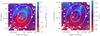 |
Fig. 1. Comparison between the absolute fluctuations Δabsolute from Eq. (8) (left) and the relative fluctuations Δrelative from Eq. (9) (right) using the surface brightness data and best fit model image of A2319. For display purposes, the images are filtered by a Gaussian kernel of 7.5″. The successive contours represent the distance to the centre in units of R500. |
with  the Fourier transform of the two-dimensional (2D) map Δ and φ the azimuthal angle on the image. The numerical evaluation of P2D, Δ is performed using the method described by Arévalo et al. (2012), which computes the variance of images filtered by Mexican hats on a characteristic scale to estimate the azimuthal average of the power spectrum. A detailed explanation of the method is provided in Appendix F. Other approaches found in the literature compute the structure function, 𝒮ℱ2D(ρ), of the image instead of the 𝒫2D(k) (e.g., Roncarelli et al. 2018; Clerc et al. 2019; Cucchetti et al. 2019). We emphasise that these two approaches are fully equivalent, since both 𝒮ℱ2D and 𝒫2D are measures of the second order correlation of the fluctuation field and are related by the following bijection, which can be derived using the Wiener–Khinchin theorem:
We stuck to the formulation in power spectrum as it is more practical in our chosen framework, in particular, to generate the density fluctuation random fields (see Sect. 2.5).
2.5. Density fluctuations as a Gaussian random field
The next step in the analysis is to properly relate 𝒫2D, Δ to the 3D power spectrum of density fluctuations. Previous work based on this method uses a proportional relationship between the 2D and 3D spectra, involving the Fourier transform of the assumed emissivity (see Eq. (11) in Churazov et al. 2012). This approximation is valid as long as the surface brightness can be considered constant, but is no longer valid when considering large areas with strong gradients and important variations in the surface brightness. Moreover, this approach does not consider the stochastic nature of this observable and the associated sample variance. To address this, we chose to consider density fluctuations as a random field. Since many works suggest deep connections between density fluctuations and turbulent processes (Zhuravleva et al. 2014; Gaspari et al. 2014; Simonte et al. 2022), we modelled the density fluctuation as a Gaussian random field (GRF) with a 3D power spectrum,  , noted with a bar to distinguish it from the 3D power spectrum measured from a single realisation of the random field. By noting ⟨.⟩ the averaging operator over realisations, it is defined as:

The link between turbulence and density fluctuations suggests both their power spectra take a similar form. As such, we adopted the simplest possible turbulent model as a Kolmogorov cascade. We chose the following functional form as proposed by ZuHone et al. (2016), which has no direction dependence under the isotropic hypothesis:
where kinj and kdisp are, respectively, the injection and dissipation scales, α is the inertial range spectral index, and  is the variance of fluctuations. For ease of understanding, we used spatial scales of injection rather than frequency scales, defined as ℓinj, dis = 1/kinj, dis and expressed in units of R500. Since the dissipation scale (of order ≳10−3R500, Brüggen et al. 2015) is expected to be much lower than the spatial resolution of our images (∼10−2R500 at the average redshift of the X-COP clusters), we set it to 10−3R500 for all X-COP clusters. This choice has little effect on the other parameters of the spectrum, since the exact value of the dissipation length will very marginally affect the normalisation of the spectrum and, therefore, σδ. The GRF hypothesis is valid as long as the fluctuations within the clusters can be represented by an isotropic homogeneous field. However, as clusters are dynamical objects, they are subject to, for instance, merging, accretion, or sloshing events at the centre, which will induce residuals that cannot be described by a GRF. This assumption is discussed further in Sect. 4.6.
2.6. Optimal definition and observable
As seen in Sect. 2.3, the definition of fluctuation and aperture size (and, more generally, the shape of the mask we choose) has various implications with regard to the signal we measure. For example, the fluctuation map, Δrel, obtained through a ratio is expected to over-represent the Poisson noise for radii ∼R500, and, conversely, for the maps, Δabs, obtained with a subtraction, the very low significance of the signal at this distance to the centre does not provide additional information. To quantify the comparison between absolute and relative approaches, we used the numerical simulations (further explained in Sect. 2.8) to study the signal-to-noise ratio (S/N) that can be obtained in each case.
We simulated 100 mock surface brightness maps for density fluctuations with σδ = 0.32, ℓinj = 0.05R500, α = 11/3 (as defined in Eq. (13)) and computed the associated 𝒫2D in the regions defined in Table 1. The maximum scale was defined using Nyquist-Shannon criterion, which is half of the highest scale accessible in the mask. For a ring of inner radius, Rmin, and outer radius, Rmax, it is given by  . To quantify the valuable information in the power spectrum, we compared it to the power spectrum that is obtained by switching off density fluctuations, 𝒩2D. This quantity represents the fluctuations which are expected when observing a perfect cluster at rest, without any density fluctuations. It can be obtained by forward modelling the power spectrum, but with a zero-normalisation density fluctuation field, accounting for the dispersion due to the mean model fit and the Poisson noise by computing it for models drawn from the posterior distribution and making various realisation of the count image. We define the S/N of the power spectrum as follows for each realisation of the mock density fluctuations:
Regions used in the analysis, minimum and maximum scale achievable in Fourier space according to Nyquist–Shannon theorem.
This quantity can trace the excess of surface brightness fluctuation when compared to what is expected with the cluster emissivity and Poisson noise. In Fig. 2, we show the comparison between the S/N obtained with the absolute method and the relative method, for the four regions of analysis and for several spatial scales. For the most central regions, the S/N metric values are high and both methods perform equivalently well. For the outermost regions, the absolute method performs better than the relative method for large spatial scales, and both perform equally well on smaller scales. With this in mind, we favour the absolute method in the following.
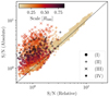 |
Fig. 2. Comparison of the S/N values obtained using the absolute and relative definition for surface brightness fluctuations, for different spatial scales and in the four regions defined in Table (1). The comparison is made for 100 mock spectra using the best-fit model and the exposure map of A3266, with density fluctuation parameters fixed at σδ = 0.32, ℓinj = 0.05R500 and α = 11/3. |
2.7. Error budget
Constraining density fluctuations requires controlling the error budget associated with surface brightness fluctuations. The Bayesian characterisation of the cluster emission (see Sect. 2.3) allows us to estimate the uncertainties related to the mean surface brightness best-fit model, in the form of posterior distribution of the model parameters. The other major source of error is the Poissonian nature of the image counts, which introduces constant power at all spatial scales.
Observables related to the velocity (or density fluctuation) field are subject to an additional variance intrinsically linked to their stochastic nature. The measured statistics of the density fluctuation field δ will vary from one realisation to another, due to finite size effects introduced by the cluster itself and the limited field of view. Any quantity that depends on δ will therefore be affected by this ‘sample variance’, including the surface brightness fluctuation power spectrum, 𝒫2D, Δ. This variance increases at higher spatial scales due to the lack of large-scale modes and becomes predominant in the error budget at spatial scales of ≳50 kpc in the structure functions of Cucchetti et al. (2019). In the following, we implement a forward modelling approach which, for the first time, accounts for the sample variance induced by the finite sizes of galaxy clusters and limited fields of view.
2.8. Simulation-based inference
The Bayesian framework is well suited to the integration of the error budget, which should be reflected in the likelihood of our problem. In a classical Bayesian inference, we seek to obtain the posterior distribution p(θ|x) of the parameters θ of our model given an observation x, by inverting the likelihood distribution p(x|θ), namely, the probability distribution of an observation given the parameters. In practice, the posterior distribution is sampled by estimating the likelihood for many parameters with Markov chain Monte Carlo (MCMC) methods. This is the process we describe in Sect. 2.3, assuming a Poisson distribution in each pixel, which allows us to define a corresponding likelihood. However, in the case of surface brightness fluctuations, there is no simple way to define an analytical and closed form for the likelihood function of a spectrum 𝒫2D, Δ given the density fluctuation parameters, as we cannot grasp the underlying distribution. Therefore, the Bayesian inference of the  parameter distributions falls under the scope of approximate Bayesian computation methods, which only require the ability to model observables x (including all the sources of variance one wishes to consider) for any set of parameters θ instead of an analytical likelihood function.
In this work, we chose to use a neural network (NN) that learns the likelihood of our problem, based on simulated observations. First, we mocked many couple of observables xi using parameters θi drawn from the prior distribution p(θ) selected for the inference. We then trained the neural network to learn an estimator q(x|θ) of the likelihood p(x|θ) using the couples (xi, θi). This approximation is accomplished by adjusting a normalising flow, which is formally an invertible bijection between two probability distributions. The normalising flow itself is built using several layers of density estimators, implemented by masked autoencoders (Germain et al. 2015), so we ended up training a masked autoregressive flow (Papamakarios et al. 2017, 2019). Once the training had converged, the posterior distribution was sampled by evaluating the likelihood with the previously trained flow, sampling for p(θ|x)∝q(x|θ)p(θ) with a classical MCMC approach.
We used the sbi library (Tejero-Cantero et al. 2020) implementation to perform this simulation-based inference. The prior distribution used for the parameters of Eq. (13) are shown in Table A.1. We generated mock X-ray images with surface brightness fluctuations by projecting an emissivity field with an additional density fluctuation field, as highlighted in Eq. (6). To achieve this, we defined emissivity cubes dimensioned as the X-COP data in the (x, y) directions and with the same spatial resolution, but expanded to ±5R500 along the line of sight. We used the same 3D models as in Sect. 2.3, that is: density, temperature, cooling, and ellipticity, along with their best-fit parameters, as well as the individual properties of each observation, that is, the exposure maps, background maps, and NH maps, to mock the expected rest surface brightness of each cluster in the X-COP sample. The density fluctuations δ are generated by drawing a single realisation of a Gaussian random field, assuming a Kolmogorov-like power spectrum, as defined in Eq. (13). These fluctuations are co-added to the modelled emissivity and projected along the line of sight in the same standard as Eq. (7). We then choose to use the S/NΔ, as defined in Eq. (14) as an observable, since this quantity reduces the proper contribution of each cluster by dividing by the spectrum of the expected emission without density fluctuations and best represents the excess power due to their presence. It is evaluated on 20 logarithmically spaced scales between the minimum and maximum scale accessible in each region, as defined in Table 1. Generating 300 000 realisations of the fluctuation field allows us to properly learn the likelihood function for each region of analysis. The posterior parameters are then sampled using the NUTS sampler, as implemented in the pyro library (Bingham et al. 2019). We checked that the number of simulations is sufficient by testing the neural network asserting proper convergence of the recovered parameters for a NN trained with an arbitrary number of simulations. We do not observe any significant improvement in training for more than 100 000 simulations.
2.9. Validation
To validate our methodology, we applied it to mock clusters with known power spectrum and statistical properties similar to the actual X-COP clusters with known density fluctuation parameters and compared them with the parameters inferred via the method outlined in Sect. 2.8, in the multiple regions defined in Table 1. We performed a validation by producing, for each mock cluster, a realisation of the density fluctuations with σδ = 0.32, ℓinj = 0.05 R500 and α = 11/3 as the parameters to recover, along with 300000 simulations for parameters drawn from the priors in Table A.1. We tackled the effect of sample variance by defining a joint likelihood for all our clusters, which is equivalent to stating that each cluster is an individual observation of the same fluctuation process. Since all spatial coordinates are scaled to R500, we can define a joint likelihood as follows:
where ℒcluster is the likelihood estimated with the previously trained NN for each cluster in the X-COP sample. The effectiveness of this approach is illustrated in Fig. 3. In this case, we randomly drew N clusters ten times to alleviate cluster selection effects on the reconstructed parameters. We computed the joint parameters for each draw and average them. The error on each parameter decreases with the number of clusters used to define the likelihood, dependence, as expected when adding independent observations.
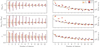 |
Fig. 3. Estimation of the posterior parameters and qualitative behaviour of the associated errors for mock observations with known parameters with an increasing number of clusters in the joint likelihood. For each point, we randomly draw N clusters ten times, compute the posterior parameter distributions and average the mean and standard deviation to alleviate the selection effect. The parameters are in each of the four regions as defined in Table (1). Left panel: mean and standard deviation of the parameters estimated for an increasing number cluster in the joint likelihood. The black line represents the true parameters. Right panel: error on each parameter compared to the number of cluster used to find the parameters, rescaled so that it is equal to 1 for N = 12. The black line shows the expected N−1/2 behaviour. |
3. Results
The data accompanying this analysis is available online on the repository2 associated with this article.
3.1. Mean profile and fluctuation maps
The marginalised parameter mean and 1σ dispersion are displayed in Tables E.1 and E.2. We ensure proper convergence of the Markov chains by computing the  statistic, as proposed in (Vehtari et al. 2021) and checking that
  . The parameters so found are compatible with those obtained by Ghirardini et al. (2019), which are representative of X-COP clusters. The corresponding fluctuation maps computed with Eq. (8) are shown in Fig. 4. Most of these fluctuation maps show non-Gaussian features in their residual. Sub-mergers or post-mergers can be identified in A2319 and A3266. Spiral-shaped structures in the inner regions of A85, A2029, or A2142 indicate the presence of gas sloshing.
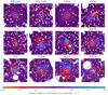 |
Fig. 4. Surface brightness fluctuation maps, Δabs, from the absolute method (see Sect. 2.6) for the X-COP cluster sample. The successive contours represent the annular regions I, II, III, and IV with outer radii of 0.1, 0.25, 0.5 and 1R500, respectively. For display purposes, the images are filtered by a Gaussian kernel of 7.5″. Each image is ∼2.5 Mpc on a side. The images are ranked in ascending order of disturbance for the cluster as measured by the CZ coefficient (see Sect. 4.1). |
3.2. Density fluctuation power spectrum parameters
We calculated, for each fluctuation map, the S/N between the surface brightness fluctuations and the fluctuations expected when only Poisson noise is present (see Sect 2.6) for the four different aforementioned regions, which is shown as a plain line in Fig. 5. Separation of the fluctuation maps into several regions provides us a way to discriminate between the different processes at work in the ICM. The central region is expected to be dominated by the presence or absence of a cool core, as well as by AGN-feedback. The second ring should be rather sensitive to the presence or not of sloshing in the core of the cluster. It is worth noting that a sloshing extending at least out to R500 has been observed in various clusters, in particular A2142 (Rossetti et al. 2013). The two outer rings should be related to the fluctuations induced by the larger dynamical assembly of the cluster, that is, by the accretion from the cosmic web and infalling halos. We also computed the S/N for the whole region inside R500 to get an average statistic on the clusters. Using the methodology presented in Sect. 2.8, we constrained the parameters of the density fluctuation power spectrum.
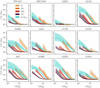 |
Fig. 5. Power spectrum S/N as defined in Eq. (14) and measured on the surface brightness fluctuation maps with the absolute method (see Sect. 2.6) in the four regions as defined in Table (1) and inside R500 for each cluster in the X-COP sample. Dotted line and shaded envelopes show the posterior distribution median and 16th–84th percentiles, accounting for the complete error budget for each cluster. The plain line represents the measured observable for each cluster in X-COP. The plots are ranked in ascending order of disturbance for the cluster, as measured by the CZ coefficient (see Sect. 4.1). |
The prior distribution and posterior median and 16th–84th percentiles are highlighted in Table A.1. The posterior probabilities for the free parameters of the 3D power spectrum derived from the joint fit over the whole X-COP sample are shown in the ‘corner plot’ of Fig. 6. We also checked the proper convergence by assessing that  for each parameter. By folding the posterior parameter distributions into our model, we obtain the resulting 2D observables accounting for the complete error budget (including the sample variance), which are shown in Fig. 5. The inner regions are marked by a high slope and low injection scale, indicating the preponderance of finite-sized structures in these regions, which corroborates with the presence of sloshing and assemblage artefacts in our fluctuation maps in Fig. 4. The estimation for all fluctuations inside R500 should be more resilient to the central region artefacts, since these structures can be described as marginal realisations of the random field when compared to the fluctuations in the external regions. The parameters in R500 jointly estimated on the whole sample converge to a normalisation of σδ ∼ 0.18, an injection of the order of ℓinj ∼ 0.4R500, with a slope of α ∼ 11/3, compatible with a pure hydrodynamical Kolmogorov cascade. This is comparable to what was determined for the Coma cluster by Schuecker et al. (2004), studying the pressure fluctuation at spatial scales between 40 and 90 kpc, as well as in Zhuravleva et al. (2015) for the Perseus cluster.
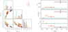 |
Fig. 6. Posterior distributions (left) and radial evolution (right) of the standard deviation, σδ, the injection scale, ℓinj, and the spectral index α of the density fluctuation power spectrum parameters, jointly evaluated on the whole X-COP cluster sample in the four regions as defined in Table (1) and within R500. The colour scale matches the four regions of interest, and the turquoise distribution represents the entire R500 region. The black dashed line represents the expected 11/3 index from Kolmogorov-Oboukhov theory. |
4. Discussions
4.1. Correlation with morphological indicators
The processes that lead to density fluctuations are expected to be related to the dynamical state of the clusters. Indeed, merger events or sloshing in the centre are intrinsically linked to the dynamic assembly of clusters and can be characterised by morphological and dynamical indicators. We consider various indicators that are well correlated with the dynamic state of the cluster (Lovisari et al. 2017; Campitiello et al. 2022) and we seek correlations with the density fluctuations parameters. We chose to use the following indicators: (1) the concentration parameter cSB compares the central emission of the cluster to its total emission. We used the definition from Campitiello et al. (2022), namely, the ratio between the surface brightness inside 0.15R500 and R500; (2) the centroid shift w relates the variation of the distance of the peak of luminosity and the centroid of the emission for a varying aperture. We used the definition and determination of this parameter from Eckert et al. (2022); (3) the Gini coefficient G measures the disparity of surface brightness in the pixels of the image. This coefficient ranges from 1 to 0 for a perfectly homogeneous and perfectly inhomogeneous distribution, respectively, and is computed using the following formula:
where si, j is the surface brightness in the i, jth pixel,  is the mean surface brightness and n the total number of pixels used to compute G; (4) finally, the Zernike moments, Zi, relate the decomposition of the image on a basis of orthogonal polynomials that allow us to efficiently describe the morphology of the cluster. Here, we specifically use the Zernike coefficient, CZ, that reflects the asymmetry of the clusters:
where  are coefficients obtained from scalar products of the image and a given Zernike polynomial, as described in Capalbo et al. (2021). The gallery of clusters in Fig. 4 is sorted by increasing CZ.
We computed these morphological indicators using all the pixels in R500, excluding the point sources and assuming spherical symmetry. We accounted for the shot noise by drawing several Poisson realisations of the measured image, with centre position drawn from our best-fit posterior distribution. The resultant morphological indicators are displayed in Table 2. We quantified the correlations by drawing 2000 values of each morphological indicators and computing the Spearman correlation coefficient with the same number of density fluctuation parameters drawn from the posterior distributions. In Fig. 7, we show the correlation matrix between the density fluctuation parameters measured inside R500 and the morphological indicators, as measured by the Spearman correlation coefficient. We observe that the best correlations appear with σδ and our 4 morphological indicators. The σδ drives the standard deviation and thus the broadness of the density fluctuation distribution. The concentration and Gini are correlated negatively with σδ, which can be understood as the fact that less concentrated clusters are generally more disturbed and therefore admit a less even distribution of its surface brightness, which goes hand in hand with the emergence of surface brightness fluctuations and thus density fluctuations. Conversely, the positive correlation with the centroid shift and the Zernike moment (which both trace the deviation of the surface brightness from a spherically symmetrical distribution) can be understood as the emergence of density and surface brightness fluctuations will disturb the symmetry of the system and therefore increase the value of these two indicators. We plot the correlation between σδ and these parameters along with the best fit as a power-law scaling in Appendix G. The range of morphological indicators we use here cannot represent the structure of the fluctuations, so it was to be expected that there would be no significant correlation with the injection scale and the spectral index. Nevertheless, they do reflect the disturbance of the surface brightness, and, in this sense, the correlation with the normalisation of the spectrum, related to the standard deviation of the fluctuations, is self-consistent.
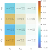 |
Fig. 7. Correlation matrix as measured by the Spearman coefficient between the morphological indicators and the density fluctuation power spectrum parameters. We display the median and difference with the 16th–84th percentiles. The morphological parameters are defined in Sect. 4.1 and the density fluctuation parameters are defined in Eq. (13) and evaluated inside R500 for each cluster in the X-COP sample. |
Concentration, cSB, centroid shift, w, Gini coefficient, G, and Zernkie moment, CZ, computed for the X-COP cluster sample, with variance from the best-fit elliptical radii and Poisson noise.
4.2. Interpretation as gas clumping
Gas clumping refers to the local deviation of the gas density from the average density expected at that location. Throughout this paper, we prefer this definition to the more specific definition of ‘accreted substructures’, so clumping defines any form of density deviation from the smooth profile. One way of interpreting our density fluctuation measure is in the form of clumping. From the 3D power spectrum of density fluctuations, we can estimate the clumping factor in our analysis regions. Similarly to Zhuravleva et al. (2015), we define the clumping factor C as follows:
where σδ is the normalisation of the density fluctuation power spectrum as defined in Eq. (13). In Fig. 8, we show the clumping factor we obtained for the regions (II), (III), and (IV) along with a comparison with the approximate clumping factor derived for 35 clusters in Eckert et al. (2015), the clumping factor estimated in the Perseus cluster with a model-free approach by de Vries et al. (2023), and the clumping factor estimated by Angelinelli et al. (2021) for the Itasca simulated cluster sample. We see a good agreement between the three results in the inner regions. We attribute our lower values to the circularly symmetric profiles used in Eckert et al. (2015). Furthermore, we see a good agreement with the factor from de Vries et al. (2023), which was computed from surface brightness fluctuations determined without a spatial surface brightness model (in contrast to what is done in this paper). This may point to the fact that accounting for the ellipticity of the surface brightness minimises the biases introduced by the arbitrary choice of model (discussed further in Sect. 4.5). However, we observe a tension in the outer region (radii ranging from 0.5 to 1 R500), which is presumably due to a change in the nature of the measured fluctuations. This is further discussed in Sects. 4.6 and 4.8.
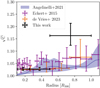 |
Fig. 8. Comparison of the clumping factor obtained with Eq. (16) for the joint fit across the X-COP sample in each annular region compared to the clumping factor obtained by Eckert et al. (2015) for a sample of 35 clusters, by de Vries et al. (2023) for the Perseus cluster and by Angelinelli et al. (2021) for 9 clusters in the ITASCA simulated clusters. The plain line and envelop represent the median and 16th–84th percentiles of the clumping factor profile. |
4.3. Interpretation as turbulent motions
Assuming that turbulence in the ICM is the main cause of measured density fluctuations, Zhuravleva et al. (2014) and Gaspari et al. (2014) have shown that the characteristic amplitude of the one-component velocity, which can be related to the 1D Mach number, ℳ1D, is proportional to the characteristic amplitude of density fluctuations. This relationship was also studied in the case of turbulence in a box and for stratified atmospheres (Mohapatra & Sharma 2019; Mohapatra et al. 2020, 2021) and is discussed further in the case of stratified turbulence in Sect. 4.7. Simonte et al. (2022) derived a similar relationship based on cosmological simulations. This relation is meant to link density fluctuations entirely to the random gas motions, which is more or less arguable depending on the relaxed or perturbed nature of the clusters. This is further discussed in Sect. 4.8. In this case, the density fluctuation dispersion σδ can be linearly related to the velocity dispersion, σv, which we refer to in terms of the 3D Mach number ℳ3D = σv/cs, where cs is the speed of sound in the ICM:

We use the relation derived for the whole sample of Simonte et al. (2022; including relaxed and disturbed clusters). This correlation was initially derived in terms of σv instead of the Mach number, which is equivalent in the limit of an isothermal ICM, but not entirely true in our study involving large scales. The turbulent Mach numbers determined for the X-COP sample are provided in Table A.1 for the four regions of analysis and in R500. The level of turbulence we measure is clearly subsonic, which agrees with the non-thermal pressure support estimated by Eckert+19 using the assumption of a universal gas fraction (Eckert et al. 2019), and also with direct measurements of spectral lines broadening (Sanders et al. 2011; The Hitomi Collaboration 2016). It is also in agreement with previous results from other works based on the statistics of fluctuation in density (Zhuravleva et al. 2015, 2018) and in thermodynamical quantities (Hofmann et al. 2016) in various galaxy clusters. We compute the one-component velocity, V1, k, as defined by Zhuravleva et al. (2018) in Eq. (4) and use the same scaling relation as proposed in Zhuravleva et al. (2014) to convert the density fluctuation to velocity:
We compare it to the results from Zhuravleva et al. (2018) for the clusters in common with X-COP in Fig 9, where we see a reasonable agreement. The source of differences between our measurements may originate from the different approach used to calculate the fluctuations, as Zhuravleva et al. (2018) used wider Chandra energy bands that are combined, whereas we use a single narrow XMM-Newton band that minimises absorption.
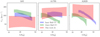 |
Fig. 9. Comparison of the one component velocity V1, k from Zhuravleva et al. (2018) in the inner and outer part of the cool-cores of each cluster, and our determination in the central region (I) as defined in Table 1. The envelope represents the 16th–84th percentiles of V1, k. |
4.4. Non-thermal pressure support
Numerical simulations predict that turbulent motions should be the dominant non-thermal pressure component in galaxy clusters (Vazza et al. 2018; Angelinelli et al. 2020). From this perspective, the aim is to characterise the ratio between the non-thermal pressure of turbulent origin and the total pressure PNTH/PTotal. This ratio can be expressed as a function of the 3D turbulent Mach number, ℳ3D (Eckert et al. 2019), and is expressed as:
where γ = 5/3 is the polytropic index. The PNTH/PTotal ratio determined for the X-COP sample are provided in Table A.1 for the four regions of analysis and inside R500. The value of PNTH/PTotal derived for the joint ℳ3D is shown in Fig. 10 as a function of radius. It is compared to the previous estimations from Eckert et al. (2019), and theoretical predictions from numerical simulation by Angelinelli et al. (2020) and Gianfagna et al. (2021). The level of non-thermal support we obtain is consistent with previous measurements on X-COP clusters at R500 (Eckert et al. 2019). Similarly to what these authors found, we determined a value that is a fraction of between 0.5 and 1R500 lower than what is predicted by numerical simulations. This discrepancy is enhanced towards the centre of clusters up to a factor of 10. In our study, the centre is filled by residual structures such as sloshing spirals and cool-cores, which dictate our measurements in these regions. This is further discussed in Sects. 4.6 and 4.8. This also could point to the fact that real clusters may be more thermalised than those predicted in numerical simulations (e.g., due to an incomplete implementation of the gas physics). In addition, other physical processes, such as cosmic rays, or magnetic fields could contribute to the non-thermal pressure support (Ruszkowski et al. 2017). However, the combination of the available radio data for clusters with radio emission and/or enough sources to study Faraday rotation allows for constraints to be set on the magnetic field pressure to ≤1 − 2%, while upper limits drawn from the non-detection of hadronic γ-rays allows putting a strong upper limit to the level of ≤1% within the virial radius of clusters. Combined, these two non-thermal pressure sources should account for ≤2 − 3% of the non-thermal pressure support on the ICM within the virial radius. Numerical estimations on the radial profile of these two components can be found in, for instance, Vazza et al. (2016). A new paper by Botteon et al. (2022) on A2255 may link turbulence at R500, or beyond, to the non-thermal pressure. With a first-order estimate, and limited to this perturbed cluster, it is argued that ∼10% of turbulent energy (compared to thermal energy) at R500 should be enough to explain the diffuse emission detected by LOFAR (assuming a Fermi II acceleration process).
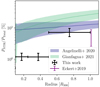 |
Fig. 10. Comparison of the fraction of turbulent to the hydrostatic pressure in the ICM as measured for the X-COP sample (black points), compared to the previous determination at R500 by Eckert et al. (2019, green point). The blue and green line and associated shade envelope shows the predictions for non-thermal pressure support from the numerical simulations by Gianfagna et al. (2021) with the MUSIC clusters and Angelinelli et al. (2020) with the ITASCA clusters. |
4.5. Density model dependency
The density model chosen arbitrarily necessarily induces fluctuations of its own, thus introducing a bias in the statistics of brightness fluctuations. We assessed the impact of the choice of model on the statistics of surface brightness fluctuations across the X-COP clusters. We compared three models corresponding to increasing level of fidelity: a circular β-model (Cavaliere & Fusco-Femiano 1976), an elliptical β-model, and our mean-model (defined in Sect. 2.3). Assuming that the surface brightness fluctuations are distributed according to a log-normal distribution (Kawahara et al. 2007), we fit a dispersion δSX inside R500:
We assume that the mean surface brightness, SX, 0, in each pixel is given, respectively, by the best-fit circular and elliptic β-model and our best-fit model (see Sect. 3 or Table A.1). The results are shown in Fig. 11. There is a systematic reduction in dispersion when a more accurate model is used, showing that the simplest way to reduce arbitrary fluctuations is to account for the elliptical shape of the surface brightness. The best improvement is the transition between the circular and elliptical β-model. This is consistent with the results by Zhuravleva et al. (2023) on numerical simulations, showing that accounting for the ellipticity of clusters can reduce the measured density fluctuations by a factor of up to 2. Moreover, we expect the underlying potential to be intrinsically triaxial (e.g., Lau et al. 2021) which motivates the smooth, elliptical surface brightness model. Including triaxiality could further improve the density modelling, but it cannot be constrained by simply using X-ray images in the [0.7–1.2] keV band. There are very few studies constraining the triaxiality using a combination of lensing, X-ray and/or Sunyaev-Zel’dovich distortion (e.g., Filippis et al. 2005; Sereno et al. 2006, 2017; Sayers et al. 2021). Applying this methodology to X-COP clusters would require a multi-wavelength modelling efforts that are beyond the scope of this paper. Generally speaking, structural residuals induced by modelling flaws affect the parameters of the power spectrum from Eq. (13). They tend to increase the normalisation as more fluctuations means more variance, change the slope due to the presence of sharp structures and affect the scale of injection, depending on the size of the residuals.
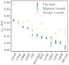 |
Fig. 11. Surface brightness deviation for a circular β-model, an elliptic β-model, and the complete model from Sect. 2.3 for each cluster in the X-COP sample |
4.6. Limitations of the Gaussian random field hypothesis
Our methodology is sensitive to density fluctuations, assumed to be homogeneous and isotropic. As such, they can be described simply by a GRF. This assumption is valid as long as the density fluctuations arise from isotropic and homogeneous turbulence, and the density fluctuations are linearly related to the turbulent velocity. In the case of the X-COP clusters, the presence of cool-cores, submergers, and sloshing causes the emergence of structures in the surface brightness fluctuations that are poorly described by a GRF. Even if these structures (e.g., sloshing) cause turbulence in the ICM (ZuHone et al. 2012), we are likely to be more sensitive to fluctuations in surface brightness generated by the spiral structure itself rather than to turbulence emerging at the interface of the two phases. The same applies to the presence of hot plasma bubbles from the central AGN feedback, which causes local gas under densities in the central regions with a characteristic size ≲10 kpc (Zhang et al. 2022). Such spatial scales are out of the reach of XMM-Newton. These rising bubbles could induce density fluctuations, exciting g-modes and sound waves. Although simulations predict that they could contribute up to 20% of the heat dissipated in the ICM, they would remain elusive in surface brightness fluctuations (Choudhury & Reynolds 2022). In contrast, in the outer regions, turbulent processes can be expected to emerge from the dynamic assembly of structures. These processes could be sustained over long periods due to the large relaxation time frames that characterise the cluster outskirts and the propensity for the emergence of magnetohydrodynamic instabilities (Perrone & Latter 2022).
We therefore expect the centre of the images to represent the clumping of the gas, that is, in our case, the overdensities present due to the dynamic assembly. Conversely, we can expect the outer regions to represent fluctuations due to turbulent phenomena, since they are not close enough to the centre of the cluster for substructure accretion to bias our results and the clearly identified substructures are masked as part of our analysis. To get rid of the presence of the structures in the centre would require either a fine modelling of the sloshing spiral, as well as the modelling of cool-cores and mergers in the surface brightness residues, or by considering a departure from Gaussianity and informed phase distribution for the random field model we fit, which is beyond the scope of this paper.
4.7. Implications of non-ideal turbulence
In galaxy clusters, the gravity influence is expected to stratify the turbulent flows. This effect will tend to suppress parallel motion and stretch the eddies in the direction orthogonal to the gravity field. Depending on the strength of the stratification, the assumption of an isotropic Gaussian field for the velocity can be rejected, since significant differences will appear between the parallel and orthogonal component (Mohapatra et al. 2020).
Furthermore, stratification will introduce a new mode of energy cascade. In addition to cascading from high to low spatial scales, kinetic energy can be converted in either direction into gravitational potential energy via buoyancy (e.g., Bolgiano 1962). By moving hot gas to regions of lower density, an additional density contrast appears and increases the total density and surface brightness fluctuations. If stratification is not negligible, not taking this effect into account may imply that the Mach number we calculate may be overestimated. The ℳ3D/σδ relationship (see Eq. (17)) proposed by Simonte et al. (2022) considers these effects in cosmological simulations and adds another degree of anisotropy by including the effect of radial accretion.
4.8. Limitations of σδ − ℳ3D equivalency
As in the previous section, it is expected that the density fluctuations observed in the centre of clusters are not necessarily representative of the turbulent phenomena taking place there. For instance, in Fig. 6, we observe both a low injection scale and high spectral index, which can be interpreted in a straightforward way as the presence of small-scale, sharp features in the fluctuation maps. The scale of injection then increases and the slope tends to reduce with the radius, reflecting the fact that these structures are less prevalent away from the centre. Previous works on turbulence based on numerical simulations shows that this radial evolution should be much lower for the velocity power spectrum (Vazza et al. 2012). Simonte et al. (2022) showed that the spectrum of density fluctuations was steeper in the centre of clusters than in the outer regions, and that its normalisation increases with the radius, while the velocity spectrum remained fairly invariant. At the same time, they showed a better correlation between density fluctuations and turbulent velocity fluctuations when using only relaxed clusters, similarly to Zhuravleva et al. (2023), while the correlation worsens when disturbed clusters, associated with a larger number of clumps in the central regions, are concerned. All together, this suggests that the density fluctuations below R500/2, are probably more sensitive to the presence of dense substructures and clumps and relatively less to the compression by turbulent motions. On the other hand, our measurement suggests that the region between R500/2 and R500 gives an overall better correlation between density and velocity fluctuations.
5. Conclusions
We performed an analysis of the spatial statistics of surface brightness fluctuations across the twelve clusters of the X-COP sample. We derived the underlying power spectrum of density fluctuations. For the first time, we have accounted for the stochastic nature of this observable by estimating the associated sample variance, thus providing a complete error budget.
-
Using a simulation-based inference approach and modelling the density fluctuations as a Kolmogorov cascade, we can constrain the normalisation, slope, and scale of injection from the surface brightness fluctuations. The increasing trend in normalisation and injection scale with distance from the cluster core is consistent, respectively, with the general idea that cluster virialisation decreases and that fluctuation-generating processes have dynamic scales that increase further away from the core.
-
We correlate the parameters of the density fluctuations with morphological indicators for X-COP clusters to find connections between dynamical state and apparent fluctuations. By properly propagating the uncertainties on each of our parameters, we found a clear correlation between the normalisation of the density fluctuation field and the four parameters of interest, suggesting a link between the measured normalisation of density fluctuations and the dynamical state of clusters. The normalisation of density fluctuations within R500 is positively correlated with the Zernike coefficient and the centroid shift, and negatively correlated with the Gini coefficient and concentration parameter. All these correlations can be interpreted as being due to the fact that the amount of fluctuation increases when the surface brightness of the cluster is disturbed, which is self-consistent in our analysis.
-
We further interpreted these density fluctuations as gas clumping and turbulent motions. We constrained the clumping factor, Mach number, and non-thermal pressure support in the different regions of interest of our clusters. We observe good agreement with clumping data from other works in the central parts, but not in the external parts, where it is ∼10% higher. On the other hand, the non-thermal pressure profile agrees with numerical simulations in the external parts and a previous determination at R500 for our sample, but is underestimated in the central parts up to a factor of 10. Due to the presence of assembly artefacts in the central regions, we discuss the notion that the density fluctuations in the central regions are dominated by pure clumping and density fluctuation originating from residual substructures, while turbulent motions dominate the outer fluctuations.
Considering the sample variance obviously increases the total error in the modelling and parametrisation of the power spectrum of fluctuations. However, this component of the error budget contributes significantly at most scales. Neglecting it could lead to over or false physical interpretations. For physical processes that are universal, such as turbulence, this sample variance can be tackled by increasing the number of sources. It is then assumed that each cluster of a sample would present an individual realisation of the same stochastic physical process, possibly rescaled with its typical size. Thus, we ought to extend our work to a larger sample to allow for a further refinement of the constraints on the velocity dispersion, slope, and injection scales, or even test a more evolved turbulence model including, such as stratification or multiple injection scales (from e.g., AGN, sloshing, dynamical assembly), while retaining sufficient statistics to study relaxed and disturbed subsets to further characterise different behaviours as a function of the source dynamical state. For instance, in a future work, we will present the application of our method to the CHEX-MATE sample (Chex-Mate Collaboration 2021).
Furthermore, upcoming and future direct measurements of turbulence will be a key step in this work and will become available in the coming years, first with the Resolve instrument on board of the XRISM missions (Terada et al. 2021) and later with the X-IFU instrument on board the Athena mission (Barret et al. 2020).
Acknowledgments
We would like to thank Giulia Gianfagna for sharing the MUSIC cluster non-thermal pressure profile from Gianfagna et al. (2021), Irina Zhuravleva for sharing the turbulent velocity power spectra from Zhuravleva et al. (2018), Matteo Angelinelli and Thomas Jones for sharing the clumping data and non-thermal pressure profile of the ITASCA cluster sample from Angelinelli et al. (2020, 2021) and Rajsekhar Mohapatra for the insightful discussions about the impact of stratification. This work was granted access to the HPC resources of CALMIP supercomputing center under the allocation 2022-22052. F.V. acknowledges financial support from the Horizon 2020 program under the ERC Starting Grant magcow, no. 714196. This work used various open-source packages such as matplotlib (Hunter 2007), astropy (Astropy Collaboration 2013, 2018), ChainConsumer (Hinton 2016), cmasher (Velden 2020), sbi (Tejero-Cantero et al. 2020), pyro (Bingham et al. 2019), jax (Bradbury et al. 2018), haiku (Hennigan et al. 2020), numpyro (Bingham et al. 2019; Phan et al. 2019).
References
- Anders, E., & Grevesse, N. 1989, Geochim. Cosmochim. Acta, 53, 197 [Google Scholar]
- Angelinelli, M., Vazza, F., Giocoli, C., et al. 2020, MNRAS, 495, 864 [NASA ADS] [CrossRef] [Google Scholar]
- Angelinelli, M., Ettori, S., Vazza, F., & Jones, T. W. 2021, A&A, 653, A171 [NASA ADS] [CrossRef] [EDP Sciences] [Google Scholar]
- Arévalo, P., Churazov, E., Zhuravleva, I., Hernández-Monteagudo, C., & Revnivtsev, M. 2012, MNRAS, 426, 1793 [CrossRef] [Google Scholar]
- Astropy Collaboration (Robitaille, T. P., et al.) 2013, A&A, 558, A33 [NASA ADS] [CrossRef] [EDP Sciences] [Google Scholar]
- Astropy Collaboration (Price-Whelan, A. M., et al.) 2018, AJ, 156, 123 [Google Scholar]
- Barret, D., Decourchelle, A., Fabian, A., et al. 2020, Astron. Nachr., 341, 224 [NASA ADS] [CrossRef] [Google Scholar]
- Bennett, J. S., & Sijacki, D. 2022, MNRAS, 514, 313 [CrossRef] [Google Scholar]
- Biffi, V., Borgani, S., Murante, G., et al. 2016, ApJ, 827, 112 [NASA ADS] [CrossRef] [Google Scholar]
- Bingham, E., Chen, J. P., Jankowiak, M., et al. 2019, J. Mach. Learn. Res., 20, 1 [Google Scholar]
- Bolgiano, R. Jr. 1962, J. Geophys. Res. (1896-1977), 67, 3015 [CrossRef] [Google Scholar]
- Botteon, A., van Weeren, R. J., Brunetti, G., et al. 2022, Sci. Adv., 8, eabq7623 [NASA ADS] [CrossRef] [Google Scholar]
- Bradbury, J., Frostig, R., Hawkins, P., et al. 2018, JAX: Composable Transformations of Python+NumPy Programs [Google Scholar]
- Brüggen, M., & Vazza, F. 2015, Astrophys. Space Sci. Lib., 407, 599 [CrossRef] [Google Scholar]
- Campitiello, M. G., Ettori, S., Lovisari, L., et al. 2022, A&A, 665, A117 [NASA ADS] [CrossRef] [EDP Sciences] [Google Scholar]
- Capalbo, V., De Petris, M., De Luca, F., et al. 2021, MNRAS, 503, 6155 [Google Scholar]
- Cappellari, M., & Copin, Y. 2003, MNRAS, 342, 345 [Google Scholar]
- Cavaliere, A., & Fusco-Femiano, R. 1976, A&A, 500, 95 [NASA ADS] [Google Scholar]
- Chex-Mate Collaboration (Arnaud, M., et al.) 2021, A&A, 650, A104 [NASA ADS] [CrossRef] [EDP Sciences] [Google Scholar]
- Choudhury, P. P., & Reynolds, C. S. 2022, MNRAS, 514, 3765 [NASA ADS] [CrossRef] [Google Scholar]
- Churazov, E., Vikhlinin, A., Zhuravleva, I., et al. 2012, MNRAS, 421, 1123 [NASA ADS] [CrossRef] [Google Scholar]
- Clerc, N., Cucchetti, E., Pointecouteau, E., & Peille, P. 2019, A&A, 629, A143 [NASA ADS] [CrossRef] [EDP Sciences] [Google Scholar]
- Cucchetti, E., Clerc, N., Pointecouteau, E., Peille, P., & Pajot, F. 2019, A&A, 629, A144 [NASA ADS] [CrossRef] [EDP Sciences] [Google Scholar]
- Cuciti, V., de Gasperin, F., Brüggen, M., et al. 2022, Nature, 609, 911 [NASA ADS] [CrossRef] [Google Scholar]
- de Vries, M., Mantz, A. B., Allen, S. W., et al. 2023, MNRAS, 518, 2954 [Google Scholar]
- Eckert, D., Roncarelli, M., Ettori, S., et al. 2015, MNRAS, 447, 2198 [Google Scholar]
- Eckert, D., Ettori, S., Pointecouteau, E., et al. 2017, Astron. Nachr., 338, 293 [Google Scholar]
- Eckert, D., Ghirardini, V., Ettori, S., et al. 2019, A&A, 621, A40 [NASA ADS] [CrossRef] [EDP Sciences] [Google Scholar]
- Eckert, D., Ettori, S., Robertson, A., et al. 2022, A&A, 666, A41 [NASA ADS] [CrossRef] [EDP Sciences] [Google Scholar]
- Ettori, S., & Eckert, D. 2022, A&A, 657, L1 [NASA ADS] [CrossRef] [EDP Sciences] [Google Scholar]
- Ettori, S., Ghirardini, V., Eckert, D., et al. 2019, A&A, 621, A39 [NASA ADS] [CrossRef] [EDP Sciences] [Google Scholar]
- Filippis, E. D., Sereno, M., Bautz, M. W., & Longo, G. 2005, ApJ, 625, 108 [NASA ADS] [CrossRef] [Google Scholar]
- Gaspari, M., Churazov, E., Nagai, D., Lau, E. T., & Zhuravleva, I. 2014, A&A, 569, A67 [NASA ADS] [CrossRef] [EDP Sciences] [Google Scholar]
- Gatuzz, E., Sanders, J. S., Canning, R., et al. 2022a, MNRAS, 513, 1932 [NASA ADS] [CrossRef] [Google Scholar]
- Gatuzz, E., Sanders, J. S., Dennerl, K., et al. 2022b, MNRAS, 511, 4511 [NASA ADS] [CrossRef] [Google Scholar]
- Germain, M., Gregor, K., Murray, I., & Larochelle, H. 2015, in Proceedings of the 32nd International Conference on Machine Learning (PMLR), 881 [Google Scholar]
- Ghirardini, V., Ettori, S., Eckert, D., et al. 2018, A&A, 614, A7 [NASA ADS] [CrossRef] [EDP Sciences] [Google Scholar]
- Ghirardini, V., Eckert, D., Ettori, S., et al. 2019, A&A, 621, A41 [NASA ADS] [CrossRef] [EDP Sciences] [Google Scholar]
- Gianfagna, G., De Petris, M., Yepes, G., et al. 2021, MNRAS, 502, 5115 [NASA ADS] [CrossRef] [Google Scholar]
- Hennigan, T., Cai, T., Norman, T., & Babuschkin, I. 2020, Haiku: Sonnet for JAX [Google Scholar]
- HI4PI Collaboration 2016, A&A, 594, A116 [NASA ADS] [CrossRef] [EDP Sciences] [Google Scholar]
- Hinton, S. 2016, J. Open Source Softw., 1, 45 [NASA ADS] [CrossRef] [Google Scholar]
- Hoffman, M. D., & Gelman, A. 2014, J. Mach. Learn. Res., 15, 1593 [Google Scholar]
- Hofmann, F., Sanders, J. S., Nandra, K., Clerc, N., & Gaspari, M. 2016, A&A, 585, A130 [NASA ADS] [CrossRef] [EDP Sciences] [Google Scholar]
- Hunter, J. D. 2007, Comput. Sci. Eng., 9, 90 [NASA ADS] [CrossRef] [Google Scholar]
- Kawahara, H., Suto, Y., Kitayama, T., et al. 2007, ApJ, 659, 257 [NASA ADS] [CrossRef] [Google Scholar]
- Khatri, R., & Gaspari, M. 2016, MNRAS, 463, 655 [Google Scholar]
- Lau, E. T., Kravtsov, A. V., & Nagai, D. 2009, ApJ, 705, 1129 [NASA ADS] [CrossRef] [Google Scholar]
- Lau, E. T., Hearin, A. P., Nagai, D., & Cappelluti, N. 2021, MNRAS, 500, 1029 [Google Scholar]
- Lovisari, L., Forman, W. R., Jones, C., et al. 2017, ApJ, 846, 51 [Google Scholar]
- McNamara, B. R., & Nulsen, P. E. J. 2012, New J. Phys., 14, 055023 [NASA ADS] [CrossRef] [Google Scholar]
- Meneghetti, M., Rasia, E., Merten, J., et al. 2010, A&A, 514, A93 [NASA ADS] [CrossRef] [EDP Sciences] [Google Scholar]
- Mohapatra, R., & Sharma, P. 2019, MNRAS, 484, 4881 [CrossRef] [Google Scholar]
- Mohapatra, R., Federrath, C., & Sharma, P. 2020, MNRAS, 493, 5838 [NASA ADS] [CrossRef] [Google Scholar]
- Mohapatra, R., Federrath, C., & Sharma, P. 2021, MNRAS, 500, 5072 [Google Scholar]
- Mori, M., & Sugihara, M. 2001, J. Comput. Appl. Math., 127, 287 [NASA ADS] [CrossRef] [Google Scholar]
- Nelson, K., Rudd, D. H., Shaw, L., & Nagai, D. 2012, ApJ, 751, 121 [NASA ADS] [CrossRef] [Google Scholar]
- Nelson, K., Lau, E. T., Nagai, D., Rudd, D. H., & Yu, L. 2014, ApJ, 782, 107 [NASA ADS] [CrossRef] [Google Scholar]
- Ota, N., Nagai, D., & Lau, E. T. 2018, PASJ, 70, 51 [NASA ADS] [CrossRef] [Google Scholar]
- Papamakarios, G., Pavlakou, T., & Murray, I. 2017, Advances in Neural Information Processing Systems (Curran Associates, Inc.), 30 [Google Scholar]
- Papamakarios, G., Sterratt, D., & Murray, I. 2019, in Proceedings of the Twenty-Second International Conference on Artificial Intelligence and Statistics (PMLR), 837 [Google Scholar]
- Perrone, L. M., & Latter, H. 2022, MNRAS, 513, 4605 [NASA ADS] [CrossRef] [Google Scholar]
- Phan, D., Pradhan, N., & Jankowiak, M. 2019, ArXiv e-prints [arXiv:1912.11554] [Google Scholar]
- Piffaretti, R., & Valdarnini, R. 2008, A&A, 491, 71 [NASA ADS] [CrossRef] [EDP Sciences] [Google Scholar]
- Pinto, C., Sanders, J. S., Werner, N., et al. 2015, A&A, 575, A38 [NASA ADS] [CrossRef] [EDP Sciences] [Google Scholar]
- Planck Collaboration XXIX. 2014, A&A, 571, A29 [NASA ADS] [CrossRef] [EDP Sciences] [Google Scholar]
- Pratt, G. W., Arnaud, M., Biviano, A., et al. 2019, Space Sci. Rev., 215, 25 [Google Scholar]
- Roncarelli, M., Gaspari, M., Ettori, S., et al. 2018, A&A, 618, A39 [NASA ADS] [CrossRef] [EDP Sciences] [Google Scholar]
- Rossetti, M., Eckert, D., Grandi, S. D., et al. 2013, A&A, 556, A44 [NASA ADS] [CrossRef] [EDP Sciences] [Google Scholar]
- Ruszkowski, M., Yang, H.-Y. K., & Reynolds, C. S. 2017, ApJ, 844, 13 [NASA ADS] [CrossRef] [Google Scholar]
- Sanders, J. S., Fabian, A. C., & Smith, R. K. 2011, MNRAS, 410, 1797 [NASA ADS] [Google Scholar]
- Sanders, J. S., Dennerl, K., Russell, H. R., et al. 2020, A&A, 633, A42 [EDP Sciences] [Google Scholar]
- Sayers, J., Sereno, M., Ettori, S., et al. 2021, MNRAS, 505, 4338 [NASA ADS] [CrossRef] [Google Scholar]
- Schuecker, P., Finoguenov, A., Miniati, F., Böhringer, H., & Briel, U. G. 2004, A&A, 426, 387 [NASA ADS] [CrossRef] [EDP Sciences] [Google Scholar]
- Sereno, M., Filippis, E. D., Longo, G., & Bautz, M. W. 2006, ApJ, 645, 170 [NASA ADS] [CrossRef] [Google Scholar]
- Sereno, M., Ettori, S., Meneghetti, M., et al. 2017, MNRAS, 467, 3801 [NASA ADS] [CrossRef] [Google Scholar]
- Shi, X., Komatsu, E., Nagai, D., & Lau, E. T. 2016, MNRAS, 455, 2936 [NASA ADS] [CrossRef] [Google Scholar]
- Simonte, M., Vazza, F., Brighenti, F., et al. 2022, A&A, 658, A149 [NASA ADS] [CrossRef] [EDP Sciences] [Google Scholar]
- Takahasi, H., & Mori, M. 1973, Publ. Res. Inst. Math. Sci., 9, 721 [CrossRef] [Google Scholar]
- Tejero-Cantero, A., Boelts, J., Deistler, M., et al. 2020, J. Open Source Softw., 5, 2505 [NASA ADS] [CrossRef] [Google Scholar]
- Terada, Y., Holland, M., Loewenstein, M., et al. 2021, J. Astron. Telesc. Instrum. Syst., 7, 037001 [NASA ADS] [CrossRef] [Google Scholar]
- The Hitomi Collaboration 2016, Nature, 535, 117 [CrossRef] [Google Scholar]
- Vazza, F., Roediger, E., & Brüggen, M. 2012, A&A, 544, A103 [NASA ADS] [CrossRef] [EDP Sciences] [Google Scholar]
- Vazza, F., Wittor, D., Brüggen, M., & Gheller, C. 2016, Galaxies, 4, 60 [NASA ADS] [CrossRef] [Google Scholar]
- Vazza, F., Angelinelli, M., Jones, T. W., et al. 2018, MNRAS, 481, L120 [NASA ADS] [CrossRef] [Google Scholar]
- Vehtari, A., Gelman, A., Simpson, D., Carpenter, B., & Bürkner, P.-C. 2021, Bayesian Anal., 16, 667 [CrossRef] [Google Scholar]
- Velden, E. v. d. 2020, J. Open Source Softw., 5, 2004 [NASA ADS] [CrossRef] [Google Scholar]
- Vikhlinin, A., Kravtsov, A., Forman, W., et al. 2006, ApJ, 640, 691 [Google Scholar]
- Voit, G. M., Meece, G., Li, Y., et al. 2017, ApJ, 845, 80 [Google Scholar]
- Weisstein, E. W. 1995, Fourier Transform (Wolfram Research, Inc.) [Google Scholar]
- XRISM Science Team 2020, ArXiv e-prints [arXiv:2003.04962] [Google Scholar]
- Zhang, C., Zhuravleva, I., Gendron-Marsolais, M.-L., et al. 2022, MNRAS, 517, 616 [CrossRef] [Google Scholar]
- Zhang, X., Simionescu, A., Gastaldello, F., et al. 2023, A&A, 672, A42 [NASA ADS] [CrossRef] [EDP Sciences] [Google Scholar]
- Zhuravleva, I., Churazov, E. M., Schekochihin, A. A., et al. 2014, ApJ, 788, L13 [Google Scholar]
- Zhuravleva, I., Churazov, E., Arévalo, P., et al. 2015, MNRAS, 450, 4184 [NASA ADS] [CrossRef] [Google Scholar]
- Zhuravleva, I., Allen, S. W., Mantz, A., & Werner, N. 2018, ApJ, 865, 53 [CrossRef] [Google Scholar]
- Zhuravleva, I., Chen, M. C., Churazov, E., et al. 2023, MNRAS, 520, 5157 [Google Scholar]
- ZuHone, J. A., Markevitch, M., Brunetti, G., & Giacintucci, S. 2012, ApJ, 762, 78 [Google Scholar]
- ZuHone, J. A., Markevitch, M., & Zhuravleva, I. 2016, ApJ, 817, 110 [NASA ADS] [CrossRef] [Google Scholar]
Appendix A: Additional table
Prior distribution, inferred median and difference with 16th-84th percentiles for the density fluctuation parameters, and deduced parameters, for each cluster in the X-COP sample and for a joint fit over the whole sample. The first section represents the density fluctuation parameters defined in Sec. 2.5. The second section corresponds to the parameters deduced from the density fluctuations, namely, the clumping factor  (Sect. 4.2), Mach number ℳ (Sect. 4.3) and ratio of non-thermal pressure to total pressure PNTH/PTOT (Sect. 4.4). The parameters of the density fluctuations as well as the inferred parameters are calculated in the four regions defined in Table (1) and within R500. We ensured the proper convergence of the MCMC sampling by assessing that
  for each parameter.
Appendix B: Fourier transform convention
In this paper, we define the Fourier transform with the classical signal processing convention, namely (0, −2π), see Weisstein (1995). This pairs results in the forward transform highlighted in Eq. B.1 and B.2. We use  and
and  to refer, respectively, to the 2D and 3D Fourier transform of a function, f.
Appendix C: Functional approximation for Ψ
The cooling function as seen by XMM-Newton in the [0.7 - 1.2] keV energy band can be phenomenologically modelled with a smooth-broken power law for the temperature dependency and an exponential absorption for the column density:
To determine the best set of parameters for this analytical approximation, we minimised the least-square of the residuals between the functional given in the previous equation and the cooling function estimated with XSPEC for each cluster of the sample. The true cooling rate is determined by computing the count rate for XMM-Newton with an PhABS*APEC model. The temperature at a given radius is set using the universal profile derived from the X-COP sample by Ghirardini et al. (2019). The exposure time is arbitrarily set to 1 Ms and split among PN, MOS-1 and MOS-2 with a 60%, 20%, 20% ratio. The abundance is fixed to 0.3 Z⊙. The count-rate in an element of volume is computed in the [0.7-1.2] keV band, assuming that ne = 1.17nH for a fully ionised ICM (Anders & Grevesse 1989), and with the following normalisation:
![$$ {\mathcal{N} } = \frac{10^{-14}}{4\pi [d_A(1+z)]^2} \int \mathrm{d} ^3V n_e n_H, $$](/articles/aa/full_html/2023/05/aa45779-22/aa45779-22-eq487.gif)
where dA is the angular diameter distance at the redshift z of the cluster. The XSPEC cooling function  is computed on a 10 × 10 grid with kBT ∈ [1, 10] keV and NH ∈ [1 × 10¹⁹, 2 × 10²¹] cm−2 to cover the ranges expected in the X-COP clusters.
Appendix D: Binning approximation
In Sect. 2.3, we make the approximation that the model counts in each bin is given by the product of the surface brightness, SX, estimated in the centre times the effective exposure ∫Binτdρ, instead of the integral over the bin geometry:
where τ is the exposure time in each pixel and dρ is a surface element of the bin area. To validate this approximation, we used a A3266 image, exposure map, and binning, and we define the relative error ϵ between the true integral and the approximation as follows:
We plot in Figure (D.1), ϵ compared to the standard deviation of τdρ within the bin. We observe that ϵ is contained around 0.5% for most of the bins. It rises to 4% for some bins located in areas of the image away from the centre, where the mosaic exposure varies greatly. These regions correspond to the places where the XMM-Newton mosaics overlap, and produce strong variations of exposure within the same bin. In any case, the bins with the coarsest approximation are those that contribute the least to the likelihood of our average model.
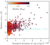 |
Fig. D.1. Evaluating the uncertainties induced by our approximation of a flat surface brightness in 2D spatial bins. The relative error, ϵ, is compared to the standard deviation of effective exposure in each bin and the color of each point indicate the distance of the bin to the centre of the cluster image. |
Appendix E: Mean model parameters
Here, we provide the parameters obtained for the average surface brightness profile, as presented in Sect. 2.3. The notation 𝒰 represents an uniform prior distribution, while 𝒩 stands for a normal distribution. The density parameters are displayed in Table E.1 and the spatial parameters are displayed in Table E.2
Mean and standard deviation of the density model parameters from Eq. 3. The prior distributions are displayed in the first line.
Mean and standard deviation of the spatial parametrisation from Eq. 5. The prior distributions are displayed in the first line.
Appendix F: Mexican hat filtering
We redirect the readers to the original article by Arévalo et al. (2012) for additional details on the Mexican hat filtering method. Here, we extend this formalism to arbitrary conventions for Fourier transforms (a, b), see Weisstein (1995). To do so, we first define the n-dimensional Fourier transform for a radially symmetric function f as the following Hankel transform:

In the following, we designate  as the N-dimension Fourier transform of f. We define the n-dimensional Gaussian kernel of σ standard deviation and its Fourier transform as follows:
The kernel of the Mexican hat is formally defined as the difference of two Gaussian kernels, whose standard deviations are, respectively,  and
and  with ϵ = 10−3. Computing the Taylor expansion of this kernel gives:

The relation between the filtered frequency kmax, which corresponds to the maximum value of the previous filter, and the standard deviation σ is given by  . We then assume that we set σ in Eq. F.4 so that kr is the frequency of maximum value. We convolve the true image I with this kernel:
The variance of the convolved image Ic is directly related to the power spectrum of I evaluated at kr, with a simple proportionality relation:  . It can be shown using Plancherel theorem:

The kernel  is supposed to be thin enough to act like a Dirac function, and be close to zero when away from kr. We can then rewrite Eq. F.6 as follows:
where  is a constant which depends on the dimension n. The idea now is to incorporate an arbitrary mask, M, to remove unwanted pixels on the image. We defined the new convolved image as follows:
Then, including these changes in Eq. F.7, we can estimate the power spectrum of the image by computing:
The integrals in Eq. F.9 are simply expressed as the sum over all cells (or pixels in 2D). This methodology intrinsically handles border effects as well as point source exclusions in the data. We test the effectiveness of this approach for an image generated via a GRF Φ, with the exposure masks of A3266. In Fig. F.1, we show a single realisation of this GRF along with the regions used to compute the power spectra, along with the distribution of their estimations for 1000 realisations of the GRF. We see a good agreement between the power spectrum used to generate the GRF and the reconstructed ones, with a slight bias, which is investigated in detail by Arévalo et al. (2012).
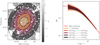 |
Fig. F.1. Assessing the efficiency of Mexican hats to compute the power spectrum of a field with arbitrary masks by computing the power spectra of 1000 realisations of a random field with known power spectrum in various ring regions. Left panel: regions of interest overplotted on a single realisation of the known random field with the A2319 exposure map. Right panel: recovered power spectra in the various regions of interest for 1000 realisations of the known random field, and comparison with the input power spectrum |
Appendix G: Correlation between σδ and the morphological indicators
Here, we show the individual correlations between the normalisation of density fluctuation estimated inside R500 and the various morphological indicators introduced in Sect. 4.1 for each cluster in the X-COP sample in Fig. G.1. We plot the best-fit distribution of a power law scaling for each correlation. This scaling is defined as log10y = a1log10x + a2. The best-fit values of a1 and a2 for each correlation are displayed in Table G.1.
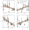 |
Fig. G.1. Correlation between σδ evaluated in R500 for each cluster and themorphological indicators defined in Sect. 4.1. The plain line and enveloprepresent the median and 16th-84th percentiles of the best fit of a power lawscaling. |
Median values of a1 and a2 and difference with the 16th-84th percentiles of the best fit for each scaling
All Tables
Regions used in the analysis, minimum and maximum scale achievable in Fourier space according to Nyquist–Shannon theorem.
Concentration, cSB, centroid shift, w, Gini coefficient, G, and Zernkie moment, CZ, computed for the X-COP cluster sample, with variance from the best-fit elliptical radii and Poisson noise.
Prior distribution, inferred median and difference with 16th-84th percentiles for the density fluctuation parameters, and deduced parameters, for each cluster in the X-COP sample and for a joint fit over the whole sample. The first section represents the density fluctuation parameters defined in Sec. 2.5. The second section corresponds to the parameters deduced from the density fluctuations, namely, the clumping factor (Sect. 4.2), Mach number ℳ (Sect. 4.3) and ratio of non-thermal pressure to total pressure PNTH/PTOT (Sect. 4.4). The parameters of the density fluctuations as well as the inferred parameters are calculated in the four regions defined in Table (1) and within R500. We ensured the proper convergence of the MCMC sampling by assessing that for each parameter.
Mean and standard deviation of the density model parameters from Eq. 3. The prior distributions are displayed in the first line.
Mean and standard deviation of the spatial parametrisation from Eq. 5. The prior distributions are displayed in the first line.
Median values of a1 and a2 and difference with the 16th-84th percentiles of the best fit for each scaling
All Figures
|
Fig. 1. Comparison between the absolute fluctuations Δabsolute from Eq. (8) (left) and the relative fluctuations Δrelative from Eq. (9) (right) using the surface brightness data and best fit model image of A2319. For display purposes, the images are filtered by a Gaussian kernel of 7.5″. The successive contours represent the distance to the centre in units of R500. |
| In the text | |
|
Fig. 2. Comparison of the S/N values obtained using the absolute and relative definition for surface brightness fluctuations, for different spatial scales and in the four regions defined in Table (1). The comparison is made for 100 mock spectra using the best-fit model and the exposure map of A3266, with density fluctuation parameters fixed at σδ = 0.32, ℓinj = 0.05R500 and α = 11/3. |
| In the text | |
|
Fig. 3. Estimation of the posterior parameters and qualitative behaviour of the associated errors for mock observations with known parameters with an increasing number of clusters in the joint likelihood. For each point, we randomly draw N clusters ten times, compute the posterior parameter distributions and average the mean and standard deviation to alleviate the selection effect. The parameters are in each of the four regions as defined in Table (1). Left panel: mean and standard deviation of the parameters estimated for an increasing number cluster in the joint likelihood. The black line represents the true parameters. Right panel: error on each parameter compared to the number of cluster used to find the parameters, rescaled so that it is equal to 1 for N = 12. The black line shows the expected N−1/2 behaviour. |
| In the text | |
|
Fig. 4. Surface brightness fluctuation maps, Δabs, from the absolute method (see Sect. 2.6) for the X-COP cluster sample. The successive contours represent the annular regions I, II, III, and IV with outer radii of 0.1, 0.25, 0.5 and 1R500, respectively. For display purposes, the images are filtered by a Gaussian kernel of 7.5″. Each image is ∼2.5 Mpc on a side. The images are ranked in ascending order of disturbance for the cluster as measured by the CZ coefficient (see Sect. 4.1). |
| In the text | |
|
Fig. 5. Power spectrum S/N as defined in Eq. (14) and measured on the surface brightness fluctuation maps with the absolute method (see Sect. 2.6) in the four regions as defined in Table (1) and inside R500 for each cluster in the X-COP sample. Dotted line and shaded envelopes show the posterior distribution median and 16th–84th percentiles, accounting for the complete error budget for each cluster. The plain line represents the measured observable for each cluster in X-COP. The plots are ranked in ascending order of disturbance for the cluster, as measured by the CZ coefficient (see Sect. 4.1). |
| In the text | |
|
Fig. 6. Posterior distributions (left) and radial evolution (right) of the standard deviation, σδ, the injection scale, ℓinj, and the spectral index α of the density fluctuation power spectrum parameters, jointly evaluated on the whole X-COP cluster sample in the four regions as defined in Table (1) and within R500. The colour scale matches the four regions of interest, and the turquoise distribution represents the entire R500 region. The black dashed line represents the expected 11/3 index from Kolmogorov-Oboukhov theory. |
| In the text | |
|
Fig. 7. Correlation matrix as measured by the Spearman coefficient between the morphological indicators and the density fluctuation power spectrum parameters. We display the median and difference with the 16th–84th percentiles. The morphological parameters are defined in Sect. 4.1 and the density fluctuation parameters are defined in Eq. (13) and evaluated inside R500 for each cluster in the X-COP sample. |
| In the text | |
|
Fig. 8. Comparison of the clumping factor obtained with Eq. (16) for the joint fit across the X-COP sample in each annular region compared to the clumping factor obtained by Eckert et al. (2015) for a sample of 35 clusters, by de Vries et al. (2023) for the Perseus cluster and by Angelinelli et al. (2021) for 9 clusters in the ITASCA simulated clusters. The plain line and envelop represent the median and 16th–84th percentiles of the clumping factor profile. |
| In the text | |
|
Fig. 9. Comparison of the one component velocity V1, k from Zhuravleva et al. (2018) in the inner and outer part of the cool-cores of each cluster, and our determination in the central region (I) as defined in Table 1. The envelope represents the 16th–84th percentiles of V1, k. |
| In the text | |
|
Fig. 10. Comparison of the fraction of turbulent to the hydrostatic pressure in the ICM as measured for the X-COP sample (black points), compared to the previous determination at R500 by Eckert et al. (2019, green point). The blue and green line and associated shade envelope shows the predictions for non-thermal pressure support from the numerical simulations by Gianfagna et al. (2021) with the MUSIC clusters and Angelinelli et al. (2020) with the ITASCA clusters. |
| In the text | |
|
Fig. 11. Surface brightness deviation for a circular β-model, an elliptic β-model, and the complete model from Sect. 2.3 for each cluster in the X-COP sample |
| In the text | |
|
Fig. D.1. Evaluating the uncertainties induced by our approximation of a flat surface brightness in 2D spatial bins. The relative error, ϵ, is compared to the standard deviation of effective exposure in each bin and the color of each point indicate the distance of the bin to the centre of the cluster image. |
| In the text | |
|
Fig. F.1. Assessing the efficiency of Mexican hats to compute the power spectrum of a field with arbitrary masks by computing the power spectra of 1000 realisations of a random field with known power spectrum in various ring regions. Left panel: regions of interest overplotted on a single realisation of the known random field with the A2319 exposure map. Right panel: recovered power spectra in the various regions of interest for 1000 realisations of the known random field, and comparison with the input power spectrum |
| In the text | |
|
Fig. G.1. Correlation between σδ evaluated in R500 for each cluster and themorphological indicators defined in Sect. 4.1. The plain line and enveloprepresent the median and 16th-84th percentiles of the best fit of a power lawscaling. |
| In the text | |
Current usage metrics show cumulative count of Article Views (full-text article views including HTML views, PDF and ePub downloads, according to the available data) and Abstracts Views on Vision4Press platform.
Data correspond to usage on the plateform after 2015. The current usage metrics is available 48-96 hours after online publication and is updated daily on week days.
Initial download of the metrics may take a while.