| Issue |
A&A
Volume 668, December 2022
|
|
|---|---|---|
| Article Number | A107 | |
| Number of page(s) | 19 | |
| Section | Cosmology (including clusters of galaxies) | |
| DOI | https://doi.org/10.1051/0004-6361/202244346 | |
| Published online | 08 December 2022 | |
Deep study of A399-401: Application of a wide-field facet calibration⋆
1
Leiden Observatory, Leiden University, PO Box 9513 2300 RA Leiden, The Netherlands
e-mail: This email address is being protected from spambots. You need JavaScript enabled to view it.
2
Dipartimento di Fisica e Astronomia, Università degli Studi di Bologna, via P. Gobetti 93/2, 40129 Bologna, Italy
3
INAF – Istituto di Radioastronomia, via P. Gobetti 101, 40129 Bologna, Italy
4
SURF/SURFsara, Science Park 140, 1098 XG Amsterdam, The Netherlands
5
ASTRON, The Netherlands Institute for Radio Astronomy, Postbus 2, 7990 AA Dwingeloo, The Netherlands
6
GEPI & USN, Observatoire de Paris, Université PSL, CNRS, 5 Place Jules Janssen, 92190 Meudon, France
7
Department of Physics & Electronics, Rhodes University, PO Box 94 Grahamstown 6140, South Africa
Received:
24
June
2022
Accepted:
24
September
2022
Abstract
Context. Diffuse synchrotron emission pervades numerous galaxy clusters, indicating the existence of cosmic rays and magnetic fields throughout the intra-cluster medium. The general consensus is that this emission is generated by shocks and turbulence that are activated during cluster merger events and cause a (re-)acceleration of particles to highly relativistic energies. Similar emission has recently been detected in megaparsec-scale filaments connecting pairs of premerging clusters. These instances are the first in which diffuse emission has been found outside of the main cluster regions.
Aims. We aim to examine the particle acceleration mechanism in the megaparsec-scale bridge between Abell 399 and Abell 401 and assess in particular whether the synchrotron emission originates from first- or second-order Fermi reacceleration. We also consider the possible influence of active galactic nuclei (AGNs).
Methods. To examine the diffuse emission and the AGNs in Abell 399 and Abell 401, we used deep (∼40 h) LOw-Frequency ARray (LOFAR) observations with an improved direction-dependent calibration to produce radio images at 144 MHz with a sensitivity of σ = 79 μJy beam−1 at a 5.9″ × 10.5″ resolution. Using a point-to-point analysis, we searched for a correlation between the radio and X-ray brightness from which we would be able to constrain the particle reacceleration mechanism.
Results. Our radio images show the radio bridge between the radio halos at high significance. We find a trend between the radio and X-ray emission in the bridge. We also measured the correlation between the radio and X-ray emission in the radio halos and find a strong correlation for Abell 401 and a weaker correlation for Abell 399. On the other hand, we measure a strong correlation for the radio halo extension from A399 in the northwest direction. With our deep images, we also find evidence for AGN particle injection and reenergized fossil plasma in the radio bridge and halos.
Conclusions. We argue that second-order Fermi reacceleration is currently the most favored process to explain the radio bridge. In addition, we find indications for a scenario in which past AGN particle injection might introduce significant scatter in the relation between the radio and X-ray emission in the bridge, but may also supply the fossil plasma needed for in situ reacceleration. The results for Abell 401 are also clearly consistent with a second-order Fermi reacceleration model. The relation between the thermal and nonthermal components in the radio halo in Abell 399 is affected by a recent merger. However, a strong correlation toward its northwest extension and the steep spectrum in the radio halo support an origin of the radio emission in a second-order Fermi reacceleration model as well. The evidence that we find for reenergized fossil plasma near Abell 399 and in the radio bridge supports the reacceleration of the fossil plasma scenario.
Key words: techniques: image processing / turbulence / radiation mechanisms: non-thermal / galaxies: clusters: intracluster medium / cosmic rays / galaxies: clusters: general
All the reduced images in this paper are only available at the CDS via anonymous ftp to cdsarc.cds.unistra.fr (130.79.128.5) or via https://cdsarc.cds.unistra.fr/viz-bin/cat/J/A+A/668/A107
© J. M. G. H. J. de Jong et al. 2022
 Open Access article, published by EDP Sciences, under the terms of the Creative Commons Attribution License (https://creativecommons.org/licenses/by/4.0), which permits unrestricted use, distribution, and reproduction in any medium, provided the original work is properly cited.
This article is published in open access under the Subscribe-to-Open model. This email address is being protected from spambots. You need JavaScript enabled to view it. to support open access publication.
1. Introduction
Structures in our Universe are growing hierarchically, with smaller systems merging to form larger structures. The largest gravitationally bound structures are galaxy clusters, and when these merge with each other, ∼1064 erg is released into the intracluster medium (ICM) on timescales of billions of years (Markevitch & Vikhlinin 2007; Hoeft et al. 2008). The ICM is a diluted plasma that permeates the cluster volume and primarily emits thermal bremsstrahlung at X-ray wavelengths. Synchrotron radio emission has been observed in numerous clusters (see van Weeren et al. 2019, for a recent review). The presence of this emission indicates the existence of cosmic rays and magnetic fields in the ICM. The general consensus is that shocks and turbulence, generated during cluster merger events, cause the (re)acceleration of particles to highly relativistic energies (Brunetti & Jones 2014). Recently, diffuse radio emission has also been detected between pairs of clusters at megaparsec (Mpc)-scales (Govoni et al. 2019; Botteon et al. 2020b). These so-called radio bridges might trace regions in which the gas is compressed during the initial phase (i.e., the premerger phase) of the collision between massive galaxy clusters. Radio observations of cluster bridges open new windows for studying the acceleration of cosmic rays in environments with a density that is lower than typical in clusters (Brunetti & Vazza 2020). The detection of radio bridges also brings us closer to the detection and study of plasma conditions in the densest phase of the so-called warm-hot intergalactic medium (WHIM; Vazza et al. 2019). However, because only a few bridges are known and only very few theory papers have been published about their possible origin, the investigation of the origin of the magnetic fields and cosmic rays in the radio bridges is still in an initial stage in these low-density environments.
Radio bridges associated with the premerging clusters Abell 1758N and Abell 1758S (A1758) at z = 0.279 (Botteon et al. 2018b, 2020b) and the premerging clusters Abell 399 and Abell 401 (A399-401) at z = 0.072 (Govoni et al. 2019) have been recently discovered. These radio bridges are between two comparable systems and were discovered with LOw Frequency ARray (LOFAR) observations at 144 MHz. Follow-up studies at different frequencies have been performed recently (Botteon et al. 2020b; Nunhokee et al. 2021). Moreover, Abell 1430 might have a radio bridge between two merging clusters (a main cluster and subcluster), but this has not been fully confirmed (Hoeft et al. 2021). Other types of radio bridges have been discovered between the Coma cluster and the NGC4839 group (z ≈ 0.0231) at 346 MHz (Kim et al. 1989) and 144 MHz (Bonafede et al. 2021) and between the cluster Abell 3562 and the radio source J 1332-3146a in the group SC 1329-313 in the Shapley supercluster (z ≈ 0.048) at GHz frequencies (Venturi et al. 2022). Of all the bridges between premerging clusters, A399-401 has been most frequently and deeply studied with X-ray observations and Sunyaev-Zeldovich (SZ) effect measurements (Fujita et al. 1996, 2008; Fabian et al. 1997; Markevitch et al. 1998; Sakelliou & Ponman 2004; Murgia et al. 2010; Planck Collaboration X 2013; Akamatsu et al. 2017; Bonjean et al. 2018; Hincks et al. 2022). It has already been known for a while that A401 has a radio halo (Harris et al. 1980; Roland et al. 1981; Bacchi et al. 2003), but Murgia et al. (2010) identified a radio halo in A399 as well, which made A399-401 the first detected double radio-halo system. The detection of these radio halos suggests that the clusters themselves are also undergoing their own mergers.
Because of energy losses, relativistic electrons can only travel up to sub-Mpc distances at 140 MHz (Jaffe 1977) in their lifetime. These age constraints mean that particles must be generated in situ to explain how diffuse radio emission can originate on Mpc scales in the A399-401 bridge. Govoni et al. (2019) proposed that radio bridges may result from first-order Fermi (Fermi-I) reacceleration of a volume-filling population of fossil relativistic electrons by weak, ℳ ≤ 2 − 3, shocks under favorable projection effects. Alternatively, Brunetti & Vazza (2020) suggested that the synchrotron emission from the radio bridge could be a result of second-order Fermi (Fermi-II) reacceleration, where turbulence plays a major role by amplifying magnetic fields and reaccelerating particles. In this case, preexisting relativistic particles and magnetic fields interact with the turbulence, which reenergizes them in the region between the two clusters. Nunhokee et al. (2021) recently constrained a steep spectrum (α > 1.5) supporting a turbulent Fermi-II reacceleration origin. Botteon et al. (2020b) found a trend between the radio and X-ray emission in the bridge A1758 by studying the spatial correlation between the two emission components. This suggests that the radio and X-ray emissions are generated in comparable volumes, which supports turbulent reacceleration. Strong spatial correlations have been observed for radio halos as well (Govoni et al. 2001; Feretti et al. 2001; Giacintucci et al. 2005; Rajpurohit et al. 2018, 2021; Botteon et al. 2020a; Ignesti et al. 2020; Biava et al. 2021; Duchesne et al. 2021; Bonafede et al. 2021), where Fermi-II reacceleration in most cases been understood to be the most relevant particle acceleration process for giant radio halos (van Weeren et al. 2019).
The goal of this paper is to study the morphology and origin of the synchrotron emission in A399-401 in more detail. We use new, deep radio data for this aim and an improved direction-dependent (DD) calibration method. With the new radio map, we study the diffuse emission from the radio halos and radio bridge in greater depth and investigate new features related to the origin of the reaccelerated particles. Additionally, we correlate our new radio surface brightness map with an X-ray surface brightness map from A399-401 as a tool for inferring the mechanism behind the reacceleration of electrons in the diffuse emission from the bridge and radio halos.
We start by describing the data and the data reduction method in Sect. 2. The radio images are discussed in Sect. 3. In Sect. 4 we consider the relation between the radio and X-ray emission. All the results are discussed in Sect. 5. Finally, we conclude our work in Sect. 6.
We use a ΛCDM cosmology model with H0 = 70 km s−1 Mpc−1, Ωm = 0.3, and ΩΛ = 0.7. The images in this paper are made in the J2000 coordinate system.
2. Observations and data reduction
In this section, we describe the radio data that we used and how we calibrated them to arrive at a final image that we used for our science. Because we wish to relate the radio and X-ray emission, we also reduced X-ray observations.
2.1. Data
For the study of A399-A401, we used 6 × 8 h of observations from LOFAR (van Haarlem et al. 2013) from project LC9_015 (PI: van Weeren). The observation IDs and observation dates are given in Table 1. Every observation has a pointing center at a right ascension of 02h 58m 21s and a declination of +13° 17′ 10″ (J2000 equinox). The data cover the frequency range from 120–168 MHz and were observed only with high-band antennas. We only used the stations located in the Netherlands. L626692 used 60 stations, while the other observations all used 62 stations.
Measurement set names with observation dates.
During the testing of our calibration method (further discussed in Sect. 2.2), we decided to flag the last 1h 20m from all the observations, which leaves a total of 40 h of observation time. This was necessary because the calibration solutions started to diverge in this part, which was most likely caused by a low elevation that decreases the sensitivity and means a thicker ionosphere to look through. Moreover, we also manually flagged a few sub-bands between 126 and 128 MHz because they were contaminated by radio frequency interference (RFI). The central frequency of our data is 144 MHz.
2.2. Calibration
The two main parts in the calibration of LOFAR data are direction-independent (DI) and DD calibration. The DI calibration follows the LOFAR Two-metre Sky Survey (LoTSS), where Prefactor version 3 with the Default Preprocessing Pipeline (DPPP) is used (van Weeren et al. 2016; Williams et al. 2016; de Gasperin et al. 2019)1. This includes RFI flagging (Offringa et al. 2012), bandpass corrections, removing data that are affected by bright off-axis sources, clock-TEC separation, polarization alignment, ionospheric rotation measure (RM) corrections, and calibrating against a sky model from external radio surveys. The implementation of the automated DI calibration pipeline itself is discussed in Mechev et al. (2017). The DI calibration has been left untouched because the main remaining calibration issues were coming from DD solutions near bright sources around the clusters.
The DD effects are caused by ionospheric effects and imperfect beam models, which can be corrected with Jones matrices (Hamaker et al. 1996; Shimwell et al. 2019), derived from the visibilities. Over time, several DD correction algorithms have been developed, for instance, SPAM (Intema et al. 2009), Sagecal (Kazemi et al. 2011), or facet calibration (van Weeren et al. 2016). For LoTSS, the DDF-Pipeline has been developed by the LOFAR Surveys Key Science Project, which is based on KillMS to derive the Jones matrices and to apply the solutions during the imaging of the entire field of view (FoV) with DDFacet (Tasse 2014; Tasse et al. 2018, 2021; Smirnov & Tasse 2015; Shimwell et al. 2019)2. With these DD calibrations, LoTSS 8-h observations reach 6″ angular resolution and a typical median sensitivity of σ ≈ 80 μJy beam−1 over the entire LoTSS-DR2 area (Shimwell et al. 2022).
Although the output from the automated DDF-Pipeline is sufficient to do most science with, there is still room for improvements, especially for targets with large angular extent. We therefore decided to further enhance the data reduction for this specific field. Our goal was to correct for artifacts around bright sources near A399 and A401, which determine how deep we can look into the substructure from the diffuse radio bridge and how much we can detect from the radio halos. One of the main parts to improve is the selection of specific directions to derive and apply DD calibrations. The DDF-Pipeline makes corrections in a user-specified number of directions (45 is used for LoTSS standard processing). The number of directions constrains the facet layout and the final calibrated image because it is assumed that the DD calibration solutions are constant throughout a facet. Because the directions are determined in an automated way, these layouts are not always optimal. This motivated us to use the recalibration method described in van Weeren et al. (2021). This calibration method has already been successfully used in numerous other works (Botteon et al. 2019, 2020a,b, 2021, 2022; Cassano et al. 2019; Hardcastle et al. 2019; Osinga et al. 2021; Hoang et al. 2021). Because A399-401 covers a large area, however, we need to apply this method for many directions, which required including additional steps. In the following sections, we describe the recipe for a single direction (N = 1) from van Weeren et al. (2021), followed by a explanation how we upgraded this to several directions (N > 1), and applied it to A399-401.
2.2.1. N = 1
First, we made a square box region with the DS9 software around a bright compact source (Joye & Mandel 2003). In this area, self-calibration was applied and DD effects were corrected for. All sources outside of this box were subtracted from the visibilities with the DD solutions and sky model from the DDF-Pipeline (extraction step, see van Weeren et al. 2021). Ideally, the box had sides with a size between 0.25° and 0.4°. Box sizes need to be large enough for the flux density to be high enough so that diverging solutions are avoided in the self-calibration, whereas to improve upon the DDF-pipeline, the boxes need to be smaller than the facets used there because both assume constant calibration solutions across the facet. After the extraction, we phase-shifted the uv-data to the center of the box and averaged the time and frequency to 16 s and 0.39 MHz to reduce the data size by a factor of 8, which is sufficient for smearing purposes and does not lead to ionospheric calibration problems. With Dysco, we further compressed the data volume (Offringa 2016). Then followed several rounds of self-calibration on the extracted box (self-calibration step). The starting point were the DI calibrations from the DDF-Pipeline. In all self-calibration rounds, we performed several so-called tecandphase calibrations with DPPP (van Diepen et al. 2018) to solve for the total electron content (TEC). We achieved this with solution intervals between 16 s and 48 s, followed by Stokes I gain calibrations with preapplied tecandphase solutions and solution intervals between 16 and 48 min along the time axis and solution intervals between 2 MHz and 6 MHz along the frequency axis. These solution intervals were automatically determined for each box region based on the amount of apparent compact source flux, as this differs per box. After all rounds of self-calibration, we created the final image of the facet. This was done with WSClean (Offringa et al. 2014) or the DDFacet imager (Tasse et al. 2018). See Fig. 1 for an example of the result after eight self-calibration cycles, imaged with WSClean.
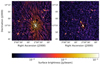 |
Fig. 1. Self-calibration of an individual box. Left panel: image of an extracted box before self-calibration and with the DI solutions alone. Right panel: image of the same region after eight self-calibration cycles. Visible artifacts around the source disappear while correcting for phase effects. These images are made with WSClean version 3 (Offringa et al. 2014). |
2.2.2. N > 1
We scaled the method in Sect. 2.2.1 in order to allow the use of an arbitrary number of box regions (N > 1). In every box, we included at least one bright source. To limit the manual steps and to save time, we implemented an automated box-region generator. We found bright sources by scanning for all pixels where the surface brightness is higher than 70 mJy beam−1 in the image with a resolution of 6″ from LoTSS that we wished to recalibrate. This pixel value was chosen because we found it to correspond to the approximate flux limit for a stable calibration for each box. We started with the brightest source and placed an initial box with a size of 0.4° ×0.4°. Because a smaller box size speeds up the self-calibration but enough flux is necessary, the algorithm optimizes the size for each box with final sizes between 0.25° and 0.4° while at the same time finding an optimal box center not farther than 0.2° from the initial position. After the full box layout was optimized, we manually further fine-tuned the result to obtain the optimal composition. This was deemed to be necessary for difficult cases in which many compact bright sources are near each other, which makes it difficult for the algorithm to decide whether to include them in different or the same boxes. When the box layout was approved (see, e.g., the left panel in Fig. 2), we followed all the same steps as in the N = 1 case for every individual box. Boxes may overlap because the solutions that are applied to a part of the sky are taken from the closest box center. In some cases, this overlap is necessary to obtain enough flux for the self-calibration. When all the individual self-calibrations were completed, we validated the quality of every set of solutions, such that no corrupt or diverging solutions were later applied in the imaging step. After the calibration, the solutions were merged into a single HDF5 solution file per observation3. The box layout can be mapped to a facet layout, as we show in Fig. 2. These facets represent the final solution area with solutions from the closest box to each pixel in the image. The solutions from these facets were applied in the final imaging step. To do this, it is only possible to use an imager that supports facets (in our case, the facet mode of WSClean version 3). All the main steps from box selection until imaging are summarized in Fig. 3.
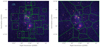 |
Fig. 2. Mapping from box layout to facet layout. Left panel: box layout for A399-401 within a radius of 0.6° from the pointing center, where all individual self-calibration boxes are contoured in green. Right panel: facet layout corresponding to the box layout from the left panel. The size of 1 Mpc is given in the top left corner for z = 0.072. |
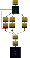 |
Fig. 3. Flowchart showing every major step from the recalibration recipe described in Sects. 2.2.1 and 2.2.2. |
2.2.3. Facet calibration for A399-401
Using the method from Sect. 2.2.2 for N > 1, we recalibrated an area with a radius of 1.2° from the pointing center of A399-401 with N = 24 boxes. This small region size was chosen to reduce the computational cost by a factor ∼4 compared to recalibrating and imaging the full field of view of our pointing4. This choice does not affect the result of our main target of interest, which is in the center of the field and extends for ∼0.5°. Everything outside this area was subtracted from the visibilities. In Fig. 2 the final box and facet layout for our field are shown. Every box corresponds to a different facet.
For A399-401 we added another reduction in the computational costs by using eight self-calibration cycles instead of the standard ten cycles for every box in van Weeren et al. (2021), as we realized that the noise level in the last two rounds of self-calibration did not reduce or there were no improvements at all. Another speedup was added by applying an additional factor 4 of time and frequency averaging in the first five rounds and by returning to the unaveraged data for the last three rounds. This did not affect the final result in a noticeable way, as we obtained similar results with or without this additional averaging. As all extractions and self-calibrations can run independent of each other on different computing nodes (i.e., it is an embarrassingly parallel problem), parellelization accelerated the total processing time with a factor ∼20. In Appendix A, we provide details about the computational cost of our recalibration.
After obtaining all self-calibration solutions, we had one merged HDF5 solution file and measurement set for each observation. These were then used for the final imaging with the facet mode from WSClean version 3, using multiscale multifrequency deconvolution and Briggs weighting in facet mode (Briggs 1995; Offringa et al. 2014; Offringa & Smirnov 2017). DDFacet also has a facet mode, but we chose WSClean because in our tests on this field, the deconvolution performs better for extended emission with this imager. Our final image had a resolution of 5.9″ × 10.5″, and we reached a sensitivity of σ = 79 μJy beam−1 at 144 MHz. We also further tapered the visibilities to obtain an image at 24.6″ × 27.1″ with σ = 230 μJy beam−1, and at 72.8″ × 75.9″ with σ = 809 μJy beam−1. These lower-resolution images have a better surface brightness sensitivity and allow us to better recover the diffuse extended emission from the radio bridge.
2.2.4. Advantages and disadvantages of recalibration
We can compare our highest-resolution recalibrated radio map with the radio map produced by the standard DDF-pipeline, which is based on the same observations. This pipeline is also used for LoTSS. By visual inspection, we see fewer artifacts around bright compact sources, and the diffuse emission is better reconstructed in our radio map than in the DDF image. We quantified this by studying the dynamic range around these compact sources. For most cases, this also improved (by a factor ∼1.6). In Appendix B we elaborate on this comparison. Overall, we can conclude that the recalibration method we used is a useful tool for calibrating a large area (larger than ∼0.8°) in which calibration artifacts remain around bright sources after using the DDF-Pipeline. However, the high additional computational costs make it a very expensive method at present (see Appendix A). The flowchart from Fig. 3 is not a full working pipeline either, which makes the implementation not straightforward. These advantages and disadvantages need to be considered or optimized in future usage of this method.
2.2.5. Removing compact sources
Because we are interested in the diffuse radio emission from the A399-401 radio bridge and radio halos and aim in Sect. 4.2 to compare this emission with an X-ray map, we also created additional images from which the contribution from discrete compact sources was removed. As there is no perfect way to do this, we applied two different methods. Both have their advantages and disadvantages.
In the first method, we start by obtaining a compact source model by making an image from which we remove the shortest baselines corresponding to a certain physical scale. This prevents extended emission from entering the model. Then, we subtract the clean components from this high-resolution model from the starting uv data. With these new uv-subtracted data, we can make an image that is tapered to a lower resolution of 72.8″ × 75.9″, where contribution from compact sources is subtracted and extended emission is enhanced. We tried several baseline cuts corresponding to 200 kpc, 300 kpc, 400 kpc, and 500 kpc at the redshift of A399-401. Based on visually inspecting and comparing the final results with the original nonsubtracted image, we decided to use the 300 kpc scale, as this gave the best balance between removing compact sources and having no noticeable impact on the diffuse emission. This corresponds to 216″ and 943λ. Although the uv-subtract method succeeds in keeping the diffuse emission and removing most of the compact sources, there are often leftover sources mainly from extended AGNs, which can affect flux density measurements.
For the second method, we use the open map filter from Rudnick (2002; the R02 filter) to remove compact sources directly in image space. This method applies a sliding minimum filter, followed by a sliding maximum filter with the same kernel size on the image data. The R02 filter is sensitive to the noise and the kernel size. This becomes more prominent when we filter in more diffuse areas with a low signal-to-noise ratio. On the other hand, this filter is very efficient in removing all compact sources smaller than the used kernel size. However, it does not remove compact sources larger than the kernel size and can leave residual emission from partially subtracted extended AGNs. By experimenting with different settings, we decided to apply this filter on our 24.6″ × 27.1″ map with a kernel size of 42″ (corresponding to 60 kpc at the redshift of A399-401) and further smooth this to 72.8″ × 75.9″ to have the same resolution as the other radio map.
2.2.6. X-ray data
We retrieved archival XMM-Newton observations of A399-401 from the Science Archive5. In particular, we made use of three pointings: 0112260101 (covering A399), 0112260301 (covering A401), and 0112260201 (covering the region between the two clusters). The European Photon Imaging Camera (EPIC) observations were processed with the XMM-Newton Scientific Analysis System (SAS v16.1.0) and the Extended Source Analysis Software (ESAS). After filtering bad time intervals due to soft proton flares, we produced an EPIC mosaic image in the 0.5 − 2.0 keV band combining the three ObsIDs. This was used to compare the X-ray and radio (from LOFAR) surface brightnesses of the observed emission. For a detailed analysis of the XMM-Newton observations, we refer to Sakelliou & Ponman (2004).
3. Results
Figures 4 and 5 present the LOFAR observation of A399-401 at three different resolutions. In Fig. 6 we show the uv-subtract and R02 filtered images, with grids and slices that are explained below. The radio map from our highest-resolution map is more than four times deeper than the 10″ radio map from Govoni et al. (2019; σ = 79 μJy beam−1 versus σ = 300 μJy beam−1). We also show zoomed images in Fig. 7, similar to Figs. S3 and S4 in Govoni et al. (2019), and use labels in Figs. 4 and 7 to mark a number of particularly interesting regions that are referred to throughout this paper.
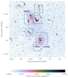 |
Fig. 4. Radio map of A399-401 at a resolution of 5.9″ × 10.5″ with σ = 79 μJy beam−1. The black highlighted regions correspond to the zoomed images in Fig. 7. The beam size is given in the lower left corner, and the scale of 1 Mpc at z = 0.072 is given in the upper left corner. The square-root color scale of the images extends from 0–25σ. |
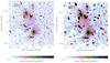 |
Fig. 5. Radio maps of the A399-401 system at lower resolutions. Left panel: resolution of 24.6″ × 27.1″ with σ = 230 μJy beam−1. Right panel: resolution 72.8″ × 75.9″ with σ = 809 μJy beam−1. The dark blue brightness depression (BD) and the halo extension (HE) are described in the text. The beam size in all images is given in the lower left corner, and the scale of 1 Mpc at z = 0.072 is given in the upper left corner. The square-root color scale of the images extends from 0 to 25σ. |
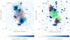 |
Fig. 6. Radio maps of A399-401 where most compact sources are removed. Left panel: radio image in blue: uv-subtract image described in the text. The square-root color scale extends from 1σ to 25σ. Green contour lines are from X-ray data from XMM-Newton, which are smoothed with a Gaussian kernel. The red slices (1100″ × 75″) point northeast. Right panel: radio image in blue: R02 filtered image described in the text. The square-root color scale of the images extends from 1σ to 25σ. It has a grid overlay on the two clusters and on the radio bridge on top of the radio image with the R02 filter. The orange grids cover the halos, the green grid covers the radio bridge, and the yellow grid covers the northwest radio halo extension from A399. The cell size in the grid is 80″ × 80″. The scale for 1 Mpc at z = 0.072 is given in both images in the upper left corner. |
3.1. Diffuse emission
In Fig. 4 we clearly detect two radio halos belonging to A401 in the north and A399 in the south. At the lower resolutions in Fig. 5, we also directly observe the diffuse emission from the radio bridge. Below we discuss the morphology of the radio bridge and halos and measure the flux densities and radio powers.
3.1.1. Morphology
In the two panels from Fig. 5, we observe a prominent brightness depression west of the bridge close to A399. We can detect this depression also from slices 1 to 5 in the radio surface brightness profile in Fig. 8, where we slice through the radio bridge images in Fig. 6 in the northeast direction for both the R02 filter and uv-subtract radio maps. We identify various compact radio sources in the bridge area, but with the exception of the sources in region D from Fig. 7, we do not detect any indication of a morphological relation between them and the radio bridge.
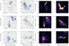 |
Fig. 7. Zoomed images of the regions in Fig. 4. These are the same sources as in Fig. S4 from Govoni et al. (2019) and ordered in the same way to facilitate comparison. Left two panels: blue contours at a resolution of 5.9″ × 10.5″ and with σ = 79 μJy beam−1, and green contours at a resolution of 72.8″ × 75.9″ and σ = 809 μJy beam−1, both at 144 MHz. Red crosses are elliptical host galaxies from the radio sources, and we label the radio components discussed in the text in brown. The background grayscale images are optical sources from Pan-STARRS DR1 (Chambers et al. 2016). Right two panels: same regions as in the left panel at 5.9″ × 10.5″ with a surface brightness color plot. The square-root color scale of the images extends 1σ to 25σ to better highlight the plasma, and the labels are the same as in the left panel in green. |
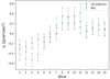 |
Fig. 8. Mean radio surface brightness from the slices from the left panel in Fig. 6, manually masked for bright AGNs, for the R02 filter and uv-subtracted radio data. The slice numbers correspond to the order of the slices in the direction from the arrow. The R02 filter removes more from the diffuse emission than the uv-subtract. Error bars include the statistic and systematic uncertainties. |
In Fig. 7 we highlight the radio halo from A401 in region C. The largest linear size (LLS) for this radio halo, measured within the 3σ contour, is 1.6 Mpc. In the region covered by the radio halo, we detect a morphologically complex bright source (C1) that has no direct optical counterpart. This structure has a straight feature with a full LLS of 300 kpc on its western and eastern side, but on its western side it, seems to connect to a bent jet-like structure (C2) that might be associated with the elliptical galaxy 2MASX J02585500+1338243 at z = 0.079 (Hill & Oegerle 1993). In region E from Fig. 7, we see the radio halo from A399. From a 3σ isophote, we find an LLS of 1.3 Mpc. In the southern area, attached to the halo, we detect a diffuse bent structure with two components with an LLS of ∼230 kpc and ∼150 kpc (E1). In the middle of these components, we can notice a small dip in the emission where we find the elliptical galaxy 2MASX J02580602+1257559 at z = 0.075 (Hill & Oegerle 1993). This dip, at the location of the optically detected galaxy, suggests that this is a switched-off radio galaxy. The radio halo also has a brightness enhancement without an optical counterpart (E2) with an LLS of ∼100 kpc. The lower resolutions in Fig. 5 show that the radio halo extends to the northwest, which we treated as a separate component for the further analysis and in the discussion in Sects. 4.2 and 5.
3.1.2. Flux densities and radio powers
To calculate the integrated flux densities for the halos, we fit the radio halos with the halo-flux density calculator (Halo-FDCA; Boxelaar et al. 2021). This software applies a Markov chain Monte Carlo (MCMC) method to fit an exponential surface brightness profile,
where I0 is the central radio surface brightness, and G(r) is a quantity related to the morphology of the halo as a function of the two-dimensional distance from the center (r). The radio power is calculated by
where DL is the luminosity distance and S144 MHz is the integrated total flux for a spectral index α. For A399 and A401, we find that a circular model with  works well, where re is the e-folding distance to the halo center. With this fit, we can estimate the flux density and radio power with corresponding uncertainties. Following Murgia et al. (2009), we decided to integrate up to 3re. For the radio halo from A399, we obtain re = 208 ± 6 kpc and find S144 MHz = 0.98 0.98 ± 0.10 Jy and P144 MHz = 0.98 0.99 ± 0.11 × 1025 W Hz−1 by using the best estimated spectral index (α = 1.75 ± 0.14; Nunhokee et al. 2021). For the radio halo in A401, we obtain re = 208 ± 7 kpc and find S144 MHz = 0.77 ± 0.08 Jy and P144 MHz = 0.99 ± 0.03 × 1025 W Hz−1 with the best estimated spectral index (α = 1.63 ± 0.07; Govoni et al. 2019). The output from Halo-FDCA is shown in Appendix C. Halo-FDCA is created for radio halos. For the radio bridge, we therefore created a manual region that we associated with the bridge (covering a similar area as the green boxes in the right panel in Fig. 6) and integrated over this area in the uv-subtract image. We obtain S144 Mhz = 0.55 ± 0.06 Jy, and by adopting the current lowest estimated spectral index for the bridge (α = 1.5; Nunhokee et al. 2021), we find P144 MHz = 0.75 ± 0.08 × 1025 W Hz−1 as the upper limit. All values are listed together in Table 2. The uncertainties include systematic, subtraction, and statistical errors. The systematic error takes into account the uncertainty of the flux scale calibration, the subtraction error takes into account the uncertainty from remaining residual emission from discrete sources after subtraction, and the statistical error takes takes into account the sensitivity of the image (see also Sect. 5 from Botteon et al. 2022).
Measured physical properties at 144 Mhz with spectral indices from Govoni et al. (2019) and Nunhokee et al. (2021).
Murgia et al. (2010) also used a circular exponential fit to calculate the flux density for the radio halo from A399. They found re = 186 ± 16 kpc at 1.4 GHz with VLA data, which is lower than but still consistent within the error bars with our value. Govoni et al. (2019) used a different radio map, with a lower resolution and sensitivity than our map (10″ and σ = 300 μJy beam−1 respectively), to measure the flux densities from the radio halos over a 5σ isophote. Despite these different methods, our values for the radio halos are consistent within the error bars with those from Govoni et al. (2019; S140 MHz = 826 ± 126.5 mJy for A401; S140 MHz = 807 ± 124.7 mJy for A399). Govoni et al. (2019) measured S140 MHz = 822 ± 147 mJy over 3.9 Mpc2 for the radio bridge. This area is a significantly larger than the 2.7 Mpc2 that we find for the bridge. Our bridge area is more conservatively chosen than Govoni et al. (2019) because they extrapolated the average surface brightness from cluster core to cluster core for the masked regions (radio halos and sources), while we excluded the radio halos from the bridge area entirely. For the average surface brightness, we both find ∼0.38 μJy arcsec−2, which means that our results (independent of the area we constrain for the bridge) are consistent with each other.
3.2. AGNs
In our radio images, we detected several interesting radio components that are associated with galaxies in or near A399-401. These bright radio sources make up a large part of all the radio emission in A399-401. We therefore discuss the radio components in our radio maps in detail. Most of the radio emission is likely associated with AGNs, as already discussed by Govoni et al. (2019). Remnant plasma from AGN are also a possible ingredient to explain the origin of the emission from the radio bridge and radio halos (this is further discussed in Sect. 5).
In region A from Fig. 7, we detect the radio galaxy (A1) corresponding to 2MASX J02581042+1351526, which was associated by Harris et al. (1980) as a probable member of A401 based on its distance to the cluster center (∼1.5 Mpc) and brightness. This object has two lobes with a full LLS of ∼300 kpc, and it is connected to diffuse emission pointed toward the A399-401 system (A2). Region B in Fig. 7 has a bright active radio core (B1) corresponding to the elliptical galaxy 87GB 025547.6+132220 at z = 0.084 (Huchra et al. 2012). Whereas there was a gap between the long tail (B2) and the core (B1) in the images from Govoni et al. (2019), we detect it as one connected structure. The radio emission from B2 has an LLS of ∼320 kpc. Connected at the end of this emission, we detect remnant plasma stretched to the west over a similar LLS of ∼270 kpc (B3). We observe signs of plasma extending southward into the radio bridge filament at the edges of B2 and B3. To the southeast of the radio halo from A401, we detect a radio galaxy (C3) in region C from Fig. 7 that we associate with 2MASX J02591487+1327117 at z = 0.078 (Hill & Oegerle 1993). Component C3 has a ∼550 kpc long prominent tail extending toward the radio halo.
In region D in Fig. 7, we detect two sources next to each other: 2MASX J02591878+1315467, located northeast at z = 0.073, and southwest from this source, we find 2MASX J02591535+1314347 at z = 0.078 (Hill & Oegerle 1993). The first is an elliptical galaxy associated with a tail with an LLS of ∼220 kpc (D1), and the second is an elliptical galaxy associated with the bright radio core to the southwest (D2) with an LLS of ∼90 kpc. From the core, a fainter component extends southwest (D3) with an LLS of ∼80 kpc and a long bent structure pointed to the south (D4). Following the same direction to the southwest, the diffuse emission again becomes brighter (D5), and in the lower-resolution images in Fig. 5, this area seems to be connected to the bridge. No optical galaxy is associated with this emission. In region F in Fig. 7, immediately below the radio halo from A399, we detect two regions with brighter plasma that lie next to each other. While the ∼250 kpc long plasma on the west side (F1) can be associated with the optical elliptical galaxy 2MASX J02580300+1251138, which is located at z = 0.075 (Hill & Oegerle 1993), we do not find an obvious optical counterpart for F2, which has about the same length. Component F1 corresponds to a tailed source, and we suspect that F2 might be the extension of F1, given its morphology (see the discussion in Sect. 5.2).
4. Thermal and nonthermal scaling relations
It has been shown observationally (e.g., Cassano et al. 2013; van Weeren et al. 2021) that the thermal emission from the ICM and nonthermal radio emission are related by the following scaling relation:

which is the relation of the radio power integrated over the entire cluster Pν at a wavelength ν and the cluster mass M derived from X-ray or SZ measurements with slope γ. It was suggested that nonthermal emission is powered by the dissipation of gravitational energy (e.g., Cassano et al. 2006).
Instead of using a statistical population of clusters to determine the thermal and nonthermal relation in the ICM by means of integrated quantities (P and M), we can also use spatially resolved quantities on single objects by inspecting the following scaling relation:

where IR is the radio surface brightness, and IX is the X-ray surface brightness with slope a. This relation has been derived for many radio halos with a point-to-point analysis (Govoni et al. 2001; Feretti et al. 2001; Giacintucci et al. 2005; Rajpurohit et al. 2018, 2021; Botteon et al. 2020a; Ignesti et al. 2020; Biava et al. 2021; Duchesne et al. 2021; Bonafede et al. 2021). A point-to-point analysis has also been performed for the radio bridge of A1758 (Botteon et al. 2020b). A strong correlation reflects the physics of the interplay between the thermal and nonthermal components (e.g., Brunetti 2004; Brunetti & Jones 2014), where the particle density and magnetic field strength (traced by the radio surface brightness) decline faster than the thermal gas density (traced by the X-ray surface brightness) if a > 1, or vice versa, if a < 1. We study these scaling relations for A399-401 below.
4.1. Mass-power relation
To determine where the radio halos from A399 and A401 are located in the cluster mass radio power diagram, we used the most recent relation at a close frequency from van Weeren et al. (2021). Following Cassano et al. (2013), they derived the following scaling relation:
for a sample of clusters in a rest-frame of P150 MHz, and where M500 is the cluster mass within a radius whithin which the average density is equal to 500 times the critical density of the Universe, taken from the PSZ2 Planck catalog (Planck Collaboration XXVII 2016). We included A399 and A401 in the figure from van Weeren et al. (2021; see Fig. 9). The radio powers from Table 2 were scaled to 150 MHz using the spectral indices from Govoni et al. (2019). To be consistent with van Weeren et al. (2021), we used the masses from Planck Collaboration XXVII (2016;  M⊙ for A399;
  M⊙ for A401). The radio halos are located close to the best-fit relation, implying that their radio powers are similar to those of other clusters with similar masses.
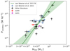 |
Fig. 9. Mass and radio power relation. The fitted regression line with a 3σ confidence interval in the shaded area and the data points in cyan come from the sample in van Weeren et al. (2021). The literature data points in black are taken, similar to van Weeren et al. (2021), from previous LOFAR and GMRT studies, and a correlation line is fit using the bivariate correlated errors and intrinsic scatter (BCES) orthogonal regression algorithm (Akritas & Bershady 1996). We left out the radio halo candidates. The radio halos A399 and A401 are added. Error bars include statistical and systematic uncertainties. |
Table 2 indicates that the radio power of the bridge is comparable to that of both of the radio halos, while we know from Hincks et al. (2022) that the mass of the bridge is only roughly 8% of the total mass of A399-401. This means that the bridge does not fit into the same mass-power relation as the radio halos, which is no surprise if bridges and radio halos have different origins through different physical mechanisms. More observations of radio bridges are needed to infer whether a different mass-power relation exists.
4.2. Point-to-point analysis
The spatial correlation between the radio and X-ray emission reflects the strength of the connection between the thermal and nonthermal components in the ICM. Therefore, a point-to-point analysis can be used as a tool for comparing the radio and X-ray emission and for obtaining information about the mechanisms of acceleration and transport of relativistic particles, and the amplification of magnetic fields in radio halos and bridges. This helps us to understand the origin of the radio bridge and halos better.
Similarly to the radio power and mass relation, we derived the radio and X-ray relation in log-log space,

where we refer to a as the slope. To quantify the correlation, we derived the Spearman correlation coefficient (rs). We used the uv-subtract and the R02 filtered map, which each have their advantages and disadvantages, as we explained in Sect. 2.2.5. We generated a grid that covers the radio bridge and radio halos separately (see the right panel in Fig. 6). There is no clear boundary between the radio halos and the radio bridge, therefore we used a 5σ radio contour around the radio halos to define the border between the radio bridge and halo areas. Furthermore, the northwestern radio halo extension from A399 and the core from A399 each have their own grids (yellow and orange, respectively) because we show below that this will help to explain the origin of the radio halo from A399. We chose a grid cell size of 80″ × 80″. This size is slightly larger than the beam size for the radio and X-ray map and therefore prevents a correlation between contiguous cells in the grid. Larger cell sizes improve the signal-to-noise ratio but reduce the number of data points for a linear regression, especially for radio halos where there is less area to cover. We calculated the average surface brightness and errors for every cell, including the statistical and systematic uncertainties for the radio and X-ray emission. From the X-ray surface brightness, we subtracted the sky background contribution, which we derived to be 1.27 ⋅ 10−7 count s−1 arcsec−2 in the 0.5–2.0 keV band. This contributes up to ∼40% of the emission at the more diffuse edge of the bridge region from A399-401. We adopted a radio surface brightness threshold of 2σ and removed cells covering areas that are not related to the radio halos or bridge, such as objects associated with AGNs, which are only partially removed in the source subtraction. The 2σ threshold is needed to prevent any effect from unreliable flux densities and noise at a low signal-to-noise ratio. Adopting a higher threshold can effectively flatten the slope values. To reduce this effect, we followed Botteon et al. (2020a) and used LIRA, which is a Bayesian regression method that allows fitting data points that have a (2σ) threshold in the y-variable (Sereno 2016)6. With this regression method, we obtain a mean and error that reflect the errors on the radio and X-ray measurements as well.
To reduce the choice sensitivity of the grid, we generated grids in a Monte Carlo (MC) fashion. This is similar to what is described in Ignesti (2022). In our approach, we made multiple grid realisations with small random offsets of 40″ at most (half of the grid resolution) around the starting and ending points of the grid. In this way, we generated 100 different grid layouts for the R02 filtered and uv-subtract radio maps. An example of a grid layout is shown in Fig. 6 (right panel). Finally, we calculated the final values and errors for the slopes and the Spearman correlation coefficients with the bootstrapping method similar to Ignesti (2022), such that we propagated the errors from individual fits to the final values. All results are presented in Table 3. The correlation plots are shown for one particular grid choice in Fig. 10.
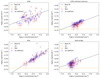 |
Fig. 10. Radio and X-ray surface brightness correlation plots for every cell from the grid used for the point-to-point analysis in the right panel of Fig. 6 for the R02 filter and uv-subtract maps. This is just one grid from the MC grid generation with 40 randomly drawn points to improve the readability of the plot. Top left panel: radio halo of A399. Top right panel: radio halo extension of A399. Lower left panel: radio halo of A401. Lower right panel: radio bridge. Error bars include the statistic and systematic uncertainties. The best linear fit with LIRA is given with a dashed black line. Only radio brightness values higher than 2σ are included. |
Correlation coefficients and slopes for  .
.
All correlations are positive and all slopes are sublinear (a < 1) in Table 3. The radio halo extension from A399 has a much steeper slope and a stronger correlation between the radio and X-ray emission than the core from A399. In Sect. 5.2 we provide more detail about this.
5. Discussion
Because radio bridges are a very recent discovery, the origin of the radio emission from these structures remains an open question. The Mpc scale size of the A399-401 radio bridge and the maximum sub-Mpc distances that relativistic particles can travel due to age constraints require an in situ mechanism as the driver of the emission of synchrotron radiation throughout the bridge region brunetti2014. An important ingredient for these models is the presence of fossil cosmic-ray electrons (e.g., Brunetti et al. 2001; Brunetti & Lazarian 2011; Petrosian 2001; Pinzke et al. 2017). These seed relativistic electrons in the energy range 100–500 MeV have a long lifetime in the ICM and can be injected by past shock activity, AGNs, galactic winds, or via the decay of charged pions from proton-proton collisions (e.g., Brunetti & Jones 2014). During merger events, fossil cosmic rays can be reaccelerated via various Fermi-I or II mechanisms and/or be reenergized by adiabatic compression (see Brunetti & Jones 2014, for a review). Evidence for the revival of AGN fossil radio plasma, for example, so-called gently reenergized tails (GReEt) and radio phoenices, has been observed in a number of clusters (e.g., de Gasperin et al. 2017; van Weeren et al. 2017; Mandal et al. 2020).
As the radio bridge is connecting the radio halos from A399 and A401, it is important to understand the origin of these radio halos as well. The fact that we observe radio halos in the center of these clusters also means that that they are also undergoing their own mergers (Buote 2001; Cassano et al. 2010).
5.1. Origin of the radio bridge
Although Govoni et al. (2019) initially suggested a model in which weak shocks reaccelerate particles via a Fermi-I type mechanism, recent studies favor a model with Fermi-II reacceleration through turbulence to explain the origin of the A399-401 radio bridge (Brunetti & Vazza 2020). With the point-to-point analysis, we find a trend between the radio and X-ray surface brightnesses, similar to Botteon et al. (2020b). We also find a source for fossil plasma, as we detect evidence for AGN injection of relativistic particles into the radio bridge region. In particular, we observe radio brightness enhancements around AGN jets that are likely places where plasma is being injected in the radio bridge. This is best visible at the southern tip of components B2 and B3 (see Fig. 7). Moreover, the plasma from A2, likely coming from an AGN (see Sect. 3.2), is pointed toward the bridge. These examples make a compelling case for the scenario in which in the past, these and other AGNs have dumped fossil plasma, which now functions as the source of primary seed electrons ready to be reaccelerated through turbulence. At the same time, the fossil plasma can scatter the radio surface brightness distribution, which in return can reduce the spatial correlation between the radio and X-ray emission. With the fossil plasma we also have an important ingredient for an in situ turbulent reacceleration model. In addition, we do not observe filamentary structures or shock surfaces in the bridge region, which is another indication that the emission is volume filling, and turbulence instead of shock models is currently the best explanation. Fermi-II reacceleration therefore remains the best candidate to explain the origin of the radio bridge. We suggest that in follow-up work, a high-resolution study of the spectral index across the bridge would be interesting to better understand the fate of the relativistic electrons that are injected into thermal gas and the role of the reacceleration processes.
An observed X-ray temperature break by Akamatsu et al. (2017) in the region that we labeled D in Fig. 7 is suggested to be a sign of an equatorial shock from the A399-401 merger axis (Ha et al. 2018) or a milder adiabatic compression between the clusters (Gu et al. 2019). Figure 7 shows that the emission from D5 is stretched in the same direction as the jet from D3, which is associated with an AGN in 2MASX J02591535+1314347. Therefore, we propose that the emission from D5 is a remnant tail from the AGN, which is reenergized by the equatorial shock or adiabatic compression. This is an alternative to the candidate radio relic classification by Govoni et al. (2019) or the switched-off radio galaxy explanation from Nunhokee et al. (2021). We further observe in Fig. 5 that the emission from D5 is directly connected with the bridge. This shows that the morphology of the radio bridge could be directly affected by this shock or compression, which can also change the spatial correlation between the radio and X-ray emission.
To determine how the values from the point-to-point analysis for A399-401 compare with other radio bridges, we considered the point-to-point analysis that was performed for the radio bridge in A1758. We used the data behind Fig. 4 from Botteon et al. (2020b) and derived a = 0.25 ± 0.08 and rs = 0.52 ± 0.22. These values are similar to what we find for the radio bridge in A399-401 (see Table 3). Although we used a finer grid resolution (∼115 kpc versus ∼185 kpc) than Botteon et al. (2020b) for A399-401, this might indicate that the two radio bridges are produced by similar processes. When we compare the slopes from these two radio bridges with mini and giant radio halos in the literature or with those from A399 and A401, we conclude that slopes from radio bridges are overall flatter (Govoni et al. 2001; Feretti et al. 2001; Giacintucci et al. 2005; Rajpurohit et al. 2018, 2021; Botteon et al. 2018b, 2020b; Ignesti et al. 2020; Biava et al. 2021; Bonafede et al. 2021, 2022). This might be an indication that the physical connections between the ICM and radio bridges and the ICM and radio halos are different from each other. More radio bridges in premerging clusters need to be studied to conclude whether these correlation and slope values are typical for radio bridges between premerging clusters, and how this relates to the underlying physical processes.
5.2. Radio halos
With our point-to-point analysis, we find a sublinear slope and a remarkable strong correlation between the radio and X-ray emission from A401. Similar to the radio bridge, we also detect AGNs that inject the radio halo environment with plasma. First of all, Fig. 7 shows that the AGN tail from C3 is directed toward the bright enhanced part in the radio halo. Second, the AGN labeled C2 affects the radio halo environment from the edges from its southern lobe. The combination of a strong radio and X-ray correlation with the observed AGN activity suggests a scenario in which turbulent Fermi-II reacceleration of fossil plasma injected by AGNs in the cluster causes most of the radio emission from this radio halo (Brunetti et al. 2008; Brunetti & Jones 2014; ZuHone et al. 2015). This is further supported by the steep spectrum (α = 1.75 ± 0.14) measured by Nunhokee et al. (2021), which can be best explained by a turbulent reacceleration mechanism in moderately disturbed systems (Brunetti et al. 2008).
We find a weaker correlation between the radio and X-ray emission for the radio halo from A399 (with and without the northwest extension) than for the radio halo from A401 with the point-to-point analysis. The relation between the radio and X-ray emission components is likely affected by the cluster merger in A399 between a higher-mass system and a lower-mass system going from east to west, as proposed by Sakelliou & Ponman (2004) and simulated by Takizawa (1999). Evidence for this merger comes from an X-ray edge at the southeast side of the cluster core of A399 (Sakelliou & Ponman 2004). The edge coincides with the region of enhanced radio brightness at the center of the radio halo, where the enhanced emission labeled E2 in Fig. 7 might be the result of a weak shock from the merger event (Murgia et al. 2010). The unrelaxed dynamical state of the cluster is reflected in the offset of the radio halo peak with respect to the X-ray peak. This is also in line with the cold front claimed by Botteon et al. (2018a). Other clusters that are in a complex merging stage show similar weaker correlations between the radio and X-ray emission from a point-to-point analysis (Shimwell et al. 2014; Duchesne et al. 2021). In contrast, we find a steeper slope and a strong radio and X-ray correlation in the northwest extension (labeled HE in the lower right panel in Fig. 5) from the radio halo. Together with steep-spectrum from Nunhokee et al. (2021), this makes a case for turbulent Fermi-II reacceleration of cosmic rays in A399, which is directed from the merger axis toward the northwest from the radio halo (Brunetti et al. 2008), and where a recent merger between a higher- and lower-mass system scatters the radio and X-ray relation around the core. The two radio tails from E1 (Fig. 7) seem to be coming from a currently switched-off AGN, as the optical source is situated in the brightness dip between these jets. Its northern jet is directly connected with the radio halo and might be a source of seed particles that are needed for the turbulent reacceleration in the radio halo. Instead, it is also possible that fossil plasma in the jets is reenergized by the currently ongoing merger in A399. Farther south of this cluster, we detect emission labeled F2 (Fig. 7), which might be a reenergized fossil plasma (originating in but disconnected from the AGN tail from 2MASX J02580300+1251138) by the merger in A399. This is again an alternative explanation to the candidate radio relic classification from Govoni et al. (2019).
6. Conclusions
A399-401 is one of a few giant intracluster radio bridges that have been observed so far (e.g., Govoni et al. 2019; Botteon et al. 2020b). We created new radio maps from A399-401 by using the improved recalibration method from van Weeren et al. (2021) and combining this with the wide-field facet imaging mode in WSClean version 3 on ∼40 h LOFAR data from six different observations. Despite the high computational costs compared to the standard DDF-Pipeline, we find that this method works well for calibrating large diffuse structures where calibration artifacts around compact sources can be an issue in reconstructing the diffuse emission with the DDF-Pipeline. In the case of A399-401, we measure improvements of a factor ∼1.6 in dynamic range for bright compact sources in our recalibrated radio map compared with the radio map produced with the DDF-Pipeline. In comparison with the previously studied radio map of A399-401 (Govoni et al. 2019), we improved the resolution from 10″ × 10″ to 5.9″ × 10.5″ and the sensitivity from 300 μJy beam−1 to 79 μJy beam−1.
By analyzing the resulting images and using a point-to-point analysis to compare the radio and X-ray surface brightness changes across a region, we find the following:
-
We clearly detect the radio halos and the radio bridge in A399-401. We report for the first time a prominent brightness depression close to the radio halo from A399, starting west of the bridge. This shows that the radio bridge is not one straight elongated structure stretching from A399 to A401.
-
We find a trend between the radio and X-ray emission for the radio bridge with a point-to-point analysis. We also detect radio surface brightness enhancements around bright AGN jets, which are an indication that fossil plasma has been left by past AGN activity. This might also scatter the radio surface brightness distribution and therefore weaken the correlation between the radio and X-ray emission in a point-to-point analysis. At the same time, this fossil plasma is necessary for in situ reacceleration. Together with the already constrained steep-spectrum (α > 1.5; Nunhokee et al. 2021) from Govoni et al. (2019), these observations make a case for Fermi-II reacceleration to explain the origin of the radio bridge.
-
We obtain similar results from the point-to-point analyses in the radio bridges in A1758 and A399-401. This suggests that these radio bridges might have similar origins.
-
By applying the point-to-point analysis to the radio halo from A401, we find a strong correlation between the radio and X-ray emission. Together with signs of AGN activity in the radio halo and its steep spectrum (α = 1.63 ± 0.07; Govoni et al. 2019), we argue that it is likely that the emission from this halo originates in Fermi-II reacceleration.
-
We see the effects of a recent merger in A399 in a weaker radio and X-ray correlation compared to what we find for A401. However, we find a strong correlation in the northwest radio halo extension. We therefore argue that this observation, together with the steep spectrum from the radio halo in A399 (α = 1.75 ± 0.14; Nunhokee et al. 2021), is in favor of a scenario in which Fermi-II reacceleration through turbulence is the main mechanism to explain the origin of the emission.
-
We suspect that the two earlier classified radio relics by Govoni et al. (2019) might be reenergized fossil plasmas from earlier AGN activity. This supports the importance of reacceleration and fossil plasma as drivers of the diffuse emission in A399-401.
Our work shows the power of refining the calibration and imaging of data from LOFAR to help us to study the diffuse emission between premerging clusters. With our results, we can conclude that reacceleration through turbulence and current and past AGN activity are likely important ingredients to explain most of the radio emission in A399-401 and possibly other radio bridges as well.
We needed 50336 CPU core hours for the recalibration (see Appendix A), which would have been ∼189000 CPU core hours for the full field of view.
Acknowledgments
This publication is part of the project CORTEX (NWA.1160.18.316) of the research programme NWA-ORC which is (partly) financed by the Dutch Research Council (NWO). This work made use of the Dutch national e-infrastructure with the support of the SURF Cooperative using grant no. EINF-1287. RJvW acknowledges support from the ERC Starting Grant ClusterWeb 804208. AB acknowledges support from the VIDI research programme with project number 639.042.729, which is financed by the Netherlands Organisation for Scientific Research (NWO), and from the ERC Starting Grant DRANOEL 714245. RC acknowledges support from INAF mainstream project ‘Galaxy Clusters Science with LOFAR’ 1.05.01.86.05. This paper is based on data obtained with the International LOFAR Telescope (ILT). LOFAR (van Haarlem et al. 2013) is the LOw Frequency ARray designed and constructed by ASTRON. It has observing, data processing, and data storage facilities in several countries, which are owned by various parties (each with their own funding sources) and are collectively operated by the ILT foundation under a joint scientific policy. The ILT resources have benefited from the following recent major funding sources: CNRS-INSU, Observatoire de Paris and Université d’Orléans, France; BMBF, MIWF-NRW, MPG, Germany; Science Foundation Ireland (SFI), Department of Business, Enterprise and Innovation (DBEI), Ireland; NWO, The Netherlands; The Science and Technology Facilities Council, UK; Ministry of Science and Higher Education, Poland; The IstitutoNazionale di Astrofisica (INAF), Italy. The Pan-STARRS1 Surveys (PS1) and the PS1 public science archive have been made possible through contributions by the Institute for Astronomy, the University of Hawaii, the Pan-STARRS Project Office, the Max-Planck Society and its participating institutes, the Max Planck Institute for Astronomy, Heidelberg and the Max Planck Institute for Extraterrestrial Physics, Garching, The Johns Hopkins University, Durham University, the University of Edinburgh, the Queen’s University Belfast, the Harvard-Smithsonian Center for Astrophysics, the Las Cumbres Observatory Global Telescope Network Incorporated, the National Central University of Taiwan, the Space Telescope Science Institute, the National Aeronautics and Space Administration under Grant No. NNX08AR22G issued through the Planetary Science Division of the NASA Science Mission Directorate, the National Science Foundation Grant No. AST-1238877, the University of Maryland, Eotvos Lorand University (ELTE), the Los Alamos National Laboratory, and the Gordon and Betty Moore Foundation. Based on observations obtained with XMM-Newton, an ESA science mission with instruments and contributions directly funded by ESA Member States and NASA.
References
- Akamatsu, H., Fujita, Y., Akahori, T., et al. 2017, in The X-ray Universe 2017, eds. J. U. Ness, & S. Migliari, 30 [Google Scholar]
- Akritas, M. G., & Bershady, M. A. 1996, ApJ, 470, 706 [Google Scholar]
- Bacchi, M., Feretti, L., Giovannini, G., & Govoni, F. 2003, A&A, 400, 465 [NASA ADS] [CrossRef] [EDP Sciences] [Google Scholar]
- Biava, N., de Gasperin, F., Bonafede, A., et al. 2021, MNRAS, 508, 3995 [NASA ADS] [CrossRef] [Google Scholar]
- Bonafede, A., Brunetti, G., Vazza, F., et al. 2021, ApJ, 907, 32 [Google Scholar]
- Bonafede, A., Brunetti, G., Rudnick, L., et al. 2022, ApJ, 933, 218 [NASA ADS] [CrossRef] [Google Scholar]
- Bonjean, V., Aghanim, N., Salomé, P., Douspis, M., & Beelen, A. 2018, A&A, 609, A49 [NASA ADS] [CrossRef] [EDP Sciences] [Google Scholar]
- Botteon, A., Shimwell, T. W., Bonafede, A., et al. 2018a, MNRAS, 478, 885 [Google Scholar]
- Botteon, A., Gastaldello, F., & Brunetti, G. 2018b, MNRAS, 476, 5591 [Google Scholar]
- Botteon, A., Cassano, R., Eckert, D., et al. 2019, A&A, 630, A77 [NASA ADS] [CrossRef] [EDP Sciences] [Google Scholar]
- Botteon, A., van Weeren, R. J., Brunetti, G., et al. 2020a, MNRAS, 499, L11 [Google Scholar]
- Botteon, A., Brunetti, G., van Weeren, R. J., et al. 2020b, ApJ, 897, 93 [Google Scholar]
- Botteon, A., Giacintucci, S., Gastaldello, F., et al. 2021, A&A, 649, A37 [NASA ADS] [CrossRef] [EDP Sciences] [Google Scholar]
- Botteon, A., Shimwell, T. W., Cassano, R., et al. 2022, A&A, 660, A78 [NASA ADS] [CrossRef] [EDP Sciences] [Google Scholar]
- Boxelaar, J. M., van Weeren, R. J., & Botteon, A. 2021, Astron. Comput., 35, 100464 [NASA ADS] [CrossRef] [Google Scholar]
- Briggs, D. S. 1995, Am. Astron. Soc. Meeting Abstr., 187, 112.02 [NASA ADS] [Google Scholar]
- Brunetti, G. 2004, J. Korean Astron. Soc., 37, 493 [NASA ADS] [CrossRef] [Google Scholar]
- Brunetti, G., & Jones, T. W. 2014, Int. J. Mod. Phys. D, 23, 1430007 [Google Scholar]
- Brunetti, G., & Lazarian, A. 2011, MNRAS, 412, 817 [NASA ADS] [Google Scholar]
- Brunetti, G., & Vazza, F. 2020, Phys. Rev. Lett., 124, 051101 [Google Scholar]
- Brunetti, G., Setti, G., Feretti, L., & Giovannini, G. 2001, New A, 6, 1 [NASA ADS] [CrossRef] [Google Scholar]
- Brunetti, G., Giacintucci, S., Cassano, R., et al. 2008, Nature, 455, 944 [Google Scholar]
- Buote, D. A. 2001, ApJ, 553, L15 [Google Scholar]
- Cassano, R., Brunetti, G., & Setti, G. 2006, MNRAS, 369, 1577 [Google Scholar]
- Cassano, R., Ettori, S., Giacintucci, S., et al. 2010, ApJ, 721, L82 [Google Scholar]
- Cassano, R., Ettori, S., Brunetti, G., et al. 2013, ApJ, 777, 141 [Google Scholar]
- Cassano, R., Botteon, A., Di Gennaro, G., et al. 2019, ApJ, 881, L18 [Google Scholar]
- Chambers, K. C., Magnier, E. A., Metcalfe, N., et al. 2016, ArXiv e-prints [arXiv:1612.05560] [Google Scholar]
- de Gasperin, F., Intema, H. T., Shimwell, T. W., et al. 2017, Sci. Adv., 3, e1701634 [Google Scholar]
- de Gasperin, F., Dijkema, T. J., Drabent, A., et al. 2019, A&A, 622, A5 [NASA ADS] [CrossRef] [EDP Sciences] [Google Scholar]
- Duchesne, S. W., Johnston-Hollitt, M., & Wilber, A. G. 2021, PASA, 38, e031 [NASA ADS] [CrossRef] [Google Scholar]
- Fabian, A. C., Peres, C. B., & White, D. A. 1997, MNRAS, 285, L35 [NASA ADS] [CrossRef] [Google Scholar]
- Feretti, L., Fusco-Femiano, R., Giovannini, G., & Govoni, F. 2001, A&A, 373, 106 [NASA ADS] [CrossRef] [EDP Sciences] [Google Scholar]
- Fujita, Y., Koyama, K., Tsuru, T., & Matsumoto, H. 1996, PASJ, 48, 191 [NASA ADS] [Google Scholar]
- Fujita, Y., Tawa, N., Hayashida, K., et al. 2008, PASJ, 60, S343 [Google Scholar]
- Giacintucci, S., Venturi, T., Brunetti, G., et al. 2005, A&A, 440, 867 [NASA ADS] [CrossRef] [EDP Sciences] [Google Scholar]
- Govoni, F., Enßlin, T. A., Feretti, L., & Giovannini, G. 2001, A&A, 369, 441 [NASA ADS] [CrossRef] [EDP Sciences] [Google Scholar]
- Govoni, F., Orrù, E., Bonafede, A., et al. 2019, Science, 364, 981 [Google Scholar]
- Gu, L., Akamatsu, H., Shimwell, T. W., et al. 2019, Nat. Astron., 3, 838 [NASA ADS] [CrossRef] [Google Scholar]
- Ha, J.-H., Ryu, D., Kang, H., & van Marle, A. J. 2018, ApJ, 864, 105 [NASA ADS] [CrossRef] [Google Scholar]
- Hamaker, J. P., Bregman, J. D., & Sault, R. J. 1996, A&AS, 117, 137 [NASA ADS] [CrossRef] [EDP Sciences] [Google Scholar]
- Hardcastle, M. J., Croston, J. H., Shimwell, T. W., et al. 2019, MNRAS, 488, 3416 [Google Scholar]
- Harris, D. E., Lari, C., Vallee, J. P., & Wilson, A. S. 1980, A&A, 42, 319 [NASA ADS] [Google Scholar]
- Hill, J. M., & Oegerle, W. R. 1993, AJ, 106, 831 [NASA ADS] [CrossRef] [Google Scholar]
- Hincks, A. D., Radiconi, F., Romero, C., et al. 2022, MNRAS, 510, 3335 [NASA ADS] [CrossRef] [Google Scholar]
- Hoang, D. N., Shimwell, T. W., Osinga, E., et al. 2021, MNRAS, 501, 576 [Google Scholar]
- Hoeft, M., Brüggen, M., Yepes, G., Gottlöber, S., & Schwope, A. 2008, MNRAS, 391, 1511 [NASA ADS] [CrossRef] [Google Scholar]
- Hoeft, M., Dumba, C., Drabent, A., et al. 2021, A&A, 654, A68 [NASA ADS] [CrossRef] [EDP Sciences] [Google Scholar]
- Huchra, J. P., Macri, L. M., Masters, K. L., et al. 2012, ApJS, 199, 26 [Google Scholar]
- Ignesti, A. 2022, New A, 92, 101732 [NASA ADS] [CrossRef] [Google Scholar]
- Ignesti, A., Brunetti, G., Gitti, M., & Giacintucci, S. 2020, A&A, 640, A37 [NASA ADS] [CrossRef] [EDP Sciences] [Google Scholar]
- Intema, H. T., van der Tol, S., Cotton, W. D., et al. 2009, A&A, 501, 1185 [NASA ADS] [CrossRef] [EDP Sciences] [Google Scholar]
- Jaffe, W. J. 1977, ApJ, 212, 1 [NASA ADS] [CrossRef] [Google Scholar]
- Joye, W. A., & Mandel, E. 2003, in Astronomical data analysis software and systems XII, 295, 489 [NASA ADS] [Google Scholar]
- Kazemi, S., Yatawatta, S., Zaroubi, S., et al. 2011, MNRAS, 414, 1656 [Google Scholar]
- Kim, K. T., Kronberg, P. P., Giovannini, G., & Venturi, T. 1989, Nature, 341, 720 [Google Scholar]
- Mandal, S., Intema, H. T., van Weeren, R. J., et al. 2020, A&A, 634, A4 [NASA ADS] [CrossRef] [EDP Sciences] [Google Scholar]
- Markevitch, M., & Vikhlinin, A. 2007, Phys. Rep., 443, 1 [Google Scholar]
- Markevitch, M., Forman, W. R., Sarazin, C. L., & Vikhlinin, A. 1998, ApJ, 503, 77 [NASA ADS] [CrossRef] [Google Scholar]
- Mechev, A., Oonk, J. B. R., Danezi, A., et al. 2017, in Proceedings of the International Symposium on Grids and Clouds (ISGC) 2017, 2 [Google Scholar]
- Murgia, M., Govoni, F., Markevitch, M., et al. 2009, A&A, 499, 679 [NASA ADS] [CrossRef] [EDP Sciences] [Google Scholar]
- Murgia, M., Govoni, F., Feretti, L., & Giovannini, G. 2010, A&A, 509, A86 [NASA ADS] [CrossRef] [EDP Sciences] [Google Scholar]
- Nunhokee, C. D., Bernardi, G., Manti, S., et al. 2021, ArXiv e-prints [arXiv:2102.02900] [Google Scholar]
- Offringa, A. R. 2016, A&A, 595, A99 [NASA ADS] [CrossRef] [EDP Sciences] [Google Scholar]
- Offringa, A. R., & Smirnov, O. 2017, MNRAS, 471, 301 [Google Scholar]
- Offringa, A. R., McKinley, B., Hurley-Walker, N., et al. 2014, MNRAS, 444, 606 [Google Scholar]
- Offringa, A. R., van de Gronde, J. J., & Roerdink, J. B. T. M. 2012, A&A, 539, A95 [NASA ADS] [CrossRef] [EDP Sciences] [Google Scholar]
- Osinga, E., van Weeren, R. J., Boxelaar, J. M., et al. 2021, A&A, 648, A11 [NASA ADS] [CrossRef] [EDP Sciences] [Google Scholar]
- Petrosian, V. 2001, ApJ, 557, 560 [Google Scholar]
- Pinzke, A., Oh, S. P., & Pfrommer, C. 2017, MNRAS, 465, 4800 [Google Scholar]
- Planck Collaboration X. 2013, A&A, 550, A134 [NASA ADS] [CrossRef] [EDP Sciences] [Google Scholar]
- Planck Collaboration XXVII. 2016, A&A, 594, A27 [NASA ADS] [CrossRef] [EDP Sciences] [Google Scholar]
- Rajpurohit, K., Hoeft, M., van Weeren, R. J., et al. 2018, ApJ, 852, 65 [Google Scholar]
- Rajpurohit, K., Brunetti, G., Bonafede, A., et al. 2021, A&A, 646, A135 [NASA ADS] [CrossRef] [EDP Sciences] [Google Scholar]
- Roland, J., Sol, H., Pauliny-Toth, I., & Witzel, A. 1981, A&A, 100, 7 [NASA ADS] [Google Scholar]
- Rudnick, L. 2002, PASP, 114, 427 [Google Scholar]
- Sakelliou, I., & Ponman, T. J. 2004, MNRAS, 351, 1439 [NASA ADS] [CrossRef] [Google Scholar]
- Sereno, M. 2016, LIRA: LInear Regression in Astronomy, Astrophysics Source Code Library [record ascl:1602.006] [Google Scholar]
- Shimwell, T. W., Brown, S., Feain, I. J., et al. 2014, MNRAS, 440, 2901 [Google Scholar]
- Shimwell, T. W., Tasse, C., Hardcastle, M. J., et al. 2019, A&A, 622, A1 [NASA ADS] [CrossRef] [EDP Sciences] [Google Scholar]
- Shimwell, T. W., Hardcastle, M. J., Tasse, C., et al. 2022, A&A, 659, A1 [NASA ADS] [CrossRef] [EDP Sciences] [Google Scholar]
- Smirnov, O. M., & Tasse, C. 2015, MNRAS, 449, 2668 [Google Scholar]
- Takizawa, M. 1999, ApJ, 520, 514 [NASA ADS] [CrossRef] [Google Scholar]
- Tasse, C. 2014, ArXiv e-prints [arXiv:1410.8706] [Google Scholar]
- Tasse, C., Hugo, B., Mirmont, M., et al. 2018, A&A, 611, A87 [NASA ADS] [CrossRef] [EDP Sciences] [Google Scholar]
- Tasse, C., Shimwell, T., Hardcastle, M. J., et al. 2021, A&A, 648, A1 [EDP Sciences] [Google Scholar]
- van Diepen, G., Dijkema, T. J., & Offringa, A. 2018, DPPP: Default Pre-Processing Pipeline, Astrophysics Source Code Library, [record ascl:1804.003] [Google Scholar]
- van Haarlem, M. P., Wise, M. W., Gunst, A. W., et al. 2013, A&A, 556, A2 [NASA ADS] [CrossRef] [EDP Sciences] [Google Scholar]
- van Weeren, R. J., Williams, W. L., Hardcastle, M. J., et al. 2016, APJS, 223, 2 [NASA ADS] [CrossRef] [Google Scholar]
- van Weeren, R. J., Andrade-Santos, F., Dawson, W. A., et al. 2017, Nat. Astron., 1, 0044 [CrossRef] [Google Scholar]
- van Weeren, R. J., de Gasperin, F., Akamatsu, H., et al. 2019, Space Sci. Rev., 215, 16 [Google Scholar]
- van Weeren, R. J., Shimwell, T. W., Botteon, A., et al. 2021, A&A, 651, A115 [NASA ADS] [CrossRef] [EDP Sciences] [Google Scholar]
- Vazza, F., Ettori, S., Roncarelli, M., et al. 2019, A&A, 627, A5 [NASA ADS] [CrossRef] [EDP Sciences] [Google Scholar]
- Venturi, T., Giacintucci, S., Merluzzi, P., et al. 2022, A&A, 660, A81 [NASA ADS] [CrossRef] [EDP Sciences] [Google Scholar]
- Williams, W. L., van Weeren, R. J., Röttgering, H. J. A., et al. 2016, MNRAS, 460, 2385 [Google Scholar]
- ZuHone, J. A., Brunetti, G., Giacintucci, S., & Markevitch, M. 2015, ApJ, 801, 146 [Google Scholar]
Appendix A: Computing recalibration
The images for A399-401 were produced with the recalibration method described in Section 2.2. We used 24 boxes within 0.6 degrees from the pointing center. All the extractions and self-calibrations were done using processor nodes on Spider7, which is a high-throughput data-processing platform from SURF8 and allows to run parallel jobs.
The total number of CPU core hours (processor units multiplied by job hours) for the recalibration is 50336. In Figure A.1 we see that the self-calibration almost used 2/3th of the total CPU core hours to process the data, while the extraction used around 1/3th. The imaging is the smallest component in the recalibration. The self-calibration and extraction step for every individual box can only be run in a serial manner, while the boxes can run in parallel of each other. This means that in the optimal case, we can speed-up with a factor of 24 for 24 boxes. However, because of the finite size of the Spider cluster and the job queue that enables sharing of the compute resources amongst many projects competing for the same resources the actual speedup achieved was a factor ∼ 20 in real time.
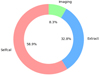 |
Fig. A.1. CPU core hours in percentage from the total amount for self-calibration, extraction, and imaging for making the image from A399-401. This is based on the calibration of A399-401 with 24 boxes within 0.6 degrees from the pointing center. |
Appendix B: DDF-Pipeline versus recalibration for A399-401
In Section 2.2 we described why we decided to use a more expensive calibration method than the automated DDF-Pipeline, which is being used by the LoTSS pipeline (Shimwell et al. 2019; Tasse et al. 2021; Shimwell et al. 2022). We compare the final image from the DDF-Pipeline with our final recalibrated image that was produced with the same observations. This is not an entirely fair one-to-one comparison, as the weighting scheme in the two methods is different because of the Briggs weighting implementation in WSClean and the DDF-Pipeline image is made with its standard 100 m baseline uv-cut. With WSClean, we obtain a resolution of 5.9″ × 10.5″, while the DDF-Pipeline uses DDFacet and has a resolution of 6″ × 6″. The resulting noise levels are similar with our σ = 79 μJy beam−1 versus DDF-Pipeline with a lower σ = 72 μJy beam−1. The individual images in Figure B.1 show that artifacts around bright compact sources are better suppressed with our calibration method in most cases, and diffuse emission is better reconstructed (a clear exception from the improvement is the right tailed source in the middle panel). To quantify the artifact reduction, we also studied several bright compact sources and found an improvement in a large dynamic range  in most cases, by a factor of ∼1.6 on average.
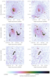 |
Fig. B.1. Image comparison between recalibration and the DDF-Pipeline. Left column: Images recalibrated with the method from this paper (see Section 2.2). Right column: Same images, produced with the DDF-Pipeline at the same color scale. The first row shows Abell 399, the second row shows Abell 401, and the last row shows the radio galaxy 2MASX J02581043+1351519 with its extended diffuse emission tail. The square-root scaled color bar extends from 0 to 25σ on average (average σ from both maps). |
Appendix C: Halo-FDCA results
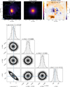 |
Fig. C.1. Results obtained from fitting the radio halo in A399 with Halo-FDCA (Boxelaar et al. 2021). Top panel: Image for the overlay fit with corresponding masks on bright AGNs. Lower panels: Markov chain Monte Carlo corner plot with the distributions of the posteriors of each fitted parameter. |
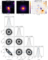 |
Fig. C.2. Results obtained from fitting the radio halo in A401 with Halo-FDCA (Boxelaar et al. 2021). Top panel: Image for the overlay fit with corresponding masks on bright AGNs. Lower panels: Markov chain Monte Carlo corner plot with the distributions of the posteriors of each fitted parameter. |
All Tables
Measured physical properties at 144 Mhz with spectral indices from Govoni et al. (2019) and Nunhokee et al. (2021).
All Figures
|
Fig. 1. Self-calibration of an individual box. Left panel: image of an extracted box before self-calibration and with the DI solutions alone. Right panel: image of the same region after eight self-calibration cycles. Visible artifacts around the source disappear while correcting for phase effects. These images are made with WSClean version 3 (Offringa et al. 2014). |
| In the text | |
|
Fig. 2. Mapping from box layout to facet layout. Left panel: box layout for A399-401 within a radius of 0.6° from the pointing center, where all individual self-calibration boxes are contoured in green. Right panel: facet layout corresponding to the box layout from the left panel. The size of 1 Mpc is given in the top left corner for z = 0.072. |
| In the text | |
|
Fig. 3. Flowchart showing every major step from the recalibration recipe described in Sects. 2.2.1 and 2.2.2. |
| In the text | |
|
Fig. 4. Radio map of A399-401 at a resolution of 5.9″ × 10.5″ with σ = 79 μJy beam−1. The black highlighted regions correspond to the zoomed images in Fig. 7. The beam size is given in the lower left corner, and the scale of 1 Mpc at z = 0.072 is given in the upper left corner. The square-root color scale of the images extends from 0–25σ. |
| In the text | |
|
Fig. 5. Radio maps of the A399-401 system at lower resolutions. Left panel: resolution of 24.6″ × 27.1″ with σ = 230 μJy beam−1. Right panel: resolution 72.8″ × 75.9″ with σ = 809 μJy beam−1. The dark blue brightness depression (BD) and the halo extension (HE) are described in the text. The beam size in all images is given in the lower left corner, and the scale of 1 Mpc at z = 0.072 is given in the upper left corner. The square-root color scale of the images extends from 0 to 25σ. |
| In the text | |
|
Fig. 6. Radio maps of A399-401 where most compact sources are removed. Left panel: radio image in blue: uv-subtract image described in the text. The square-root color scale extends from 1σ to 25σ. Green contour lines are from X-ray data from XMM-Newton, which are smoothed with a Gaussian kernel. The red slices (1100″ × 75″) point northeast. Right panel: radio image in blue: R02 filtered image described in the text. The square-root color scale of the images extends from 1σ to 25σ. It has a grid overlay on the two clusters and on the radio bridge on top of the radio image with the R02 filter. The orange grids cover the halos, the green grid covers the radio bridge, and the yellow grid covers the northwest radio halo extension from A399. The cell size in the grid is 80″ × 80″. The scale for 1 Mpc at z = 0.072 is given in both images in the upper left corner. |
| In the text | |
|
Fig. 7. Zoomed images of the regions in Fig. 4. These are the same sources as in Fig. S4 from Govoni et al. (2019) and ordered in the same way to facilitate comparison. Left two panels: blue contours at a resolution of 5.9″ × 10.5″ and with σ = 79 μJy beam−1, and green contours at a resolution of 72.8″ × 75.9″ and σ = 809 μJy beam−1, both at 144 MHz. Red crosses are elliptical host galaxies from the radio sources, and we label the radio components discussed in the text in brown. The background grayscale images are optical sources from Pan-STARRS DR1 (Chambers et al. 2016). Right two panels: same regions as in the left panel at 5.9″ × 10.5″ with a surface brightness color plot. The square-root color scale of the images extends 1σ to 25σ to better highlight the plasma, and the labels are the same as in the left panel in green. |
| In the text | |
|
Fig. 8. Mean radio surface brightness from the slices from the left panel in Fig. 6, manually masked for bright AGNs, for the R02 filter and uv-subtracted radio data. The slice numbers correspond to the order of the slices in the direction from the arrow. The R02 filter removes more from the diffuse emission than the uv-subtract. Error bars include the statistic and systematic uncertainties. |
| In the text | |
|
Fig. 9. Mass and radio power relation. The fitted regression line with a 3σ confidence interval in the shaded area and the data points in cyan come from the sample in van Weeren et al. (2021). The literature data points in black are taken, similar to van Weeren et al. (2021), from previous LOFAR and GMRT studies, and a correlation line is fit using the bivariate correlated errors and intrinsic scatter (BCES) orthogonal regression algorithm (Akritas & Bershady 1996). We left out the radio halo candidates. The radio halos A399 and A401 are added. Error bars include statistical and systematic uncertainties. |
| In the text | |
|
Fig. 10. Radio and X-ray surface brightness correlation plots for every cell from the grid used for the point-to-point analysis in the right panel of Fig. 6 for the R02 filter and uv-subtract maps. This is just one grid from the MC grid generation with 40 randomly drawn points to improve the readability of the plot. Top left panel: radio halo of A399. Top right panel: radio halo extension of A399. Lower left panel: radio halo of A401. Lower right panel: radio bridge. Error bars include the statistic and systematic uncertainties. The best linear fit with LIRA is given with a dashed black line. Only radio brightness values higher than 2σ are included. |
| In the text | |
|
Fig. A.1. CPU core hours in percentage from the total amount for self-calibration, extraction, and imaging for making the image from A399-401. This is based on the calibration of A399-401 with 24 boxes within 0.6 degrees from the pointing center. |
| In the text | |
|
Fig. B.1. Image comparison between recalibration and the DDF-Pipeline. Left column: Images recalibrated with the method from this paper (see Section 2.2). Right column: Same images, produced with the DDF-Pipeline at the same color scale. The first row shows Abell 399, the second row shows Abell 401, and the last row shows the radio galaxy 2MASX J02581043+1351519 with its extended diffuse emission tail. The square-root scaled color bar extends from 0 to 25σ on average (average σ from both maps). |
| In the text | |
|
Fig. C.1. Results obtained from fitting the radio halo in A399 with Halo-FDCA (Boxelaar et al. 2021). Top panel: Image for the overlay fit with corresponding masks on bright AGNs. Lower panels: Markov chain Monte Carlo corner plot with the distributions of the posteriors of each fitted parameter. |
| In the text | |
|
Fig. C.2. Results obtained from fitting the radio halo in A401 with Halo-FDCA (Boxelaar et al. 2021). Top panel: Image for the overlay fit with corresponding masks on bright AGNs. Lower panels: Markov chain Monte Carlo corner plot with the distributions of the posteriors of each fitted parameter. |
| In the text | |
Current usage metrics show cumulative count of Article Views (full-text article views including HTML views, PDF and ePub downloads, according to the available data) and Abstracts Views on Vision4Press platform.
Data correspond to usage on the plateform after 2015. The current usage metrics is available 48-96 hours after online publication and is updated daily on week days.
Initial download of the metrics may take a while.