| Issue |
A&A
Volume 682, February 2024
|
|
|---|---|---|
| Article Number | A105 | |
| Number of page(s) | 11 | |
| Section | Cosmology (including clusters of galaxies) | |
| DOI | https://doi.org/10.1051/0004-6361/202346243 | |
| Published online | 07 February 2024 | |
Probing diffuse radio emission in bridges between galaxy clusters with uGMRT⋆
1
Dipartimento di Fisica e Astronomia, Università degli Studi di Bologna, Via P. Gobetti 93/2, 40129 Bologna, Italy
e-mail: This email address is being protected from spambots. You need JavaScript enabled to view it.
2
INAF – Istituto di Radioastronomia, Via P. Gobetti 101, 40129 Bologna, Italy
3
Department of Physics and Electronics, Rhodes University, PO Box 94 Makhanda 6140, South Africa
4
South African Radio Astronomy Observatory (SARAO), Black River Park, 2 Fir Street, Observatory, Cape Town 7925, South Africa
5
CSIRO Space & Astronomy, PO Box 1130 Bentley, WA 6102, Australia
Received:
24
February
2023
Accepted:
14
November
2023
Abstract
Aims. Recent X-ray and Sunyaev–Zeldovich (SZ) observations have detected thermal emission between early-stage merging galaxy clusters. The main purpose of this work is to investigate the properties of the non-thermal emission in the interacting cluster pairs Abell 0399-Abell 0401 and Abell 21-PSZ2 G114.9.
Methods. These two unique cluster pairs have been found in an interacting state. In both cases, their connection along a filament is supported by an SZ effect detected by the Planck satellite and, in the special case of Abell 0399-Abell 0401, the presence of a radio bridge has been already confirmed by LOFAR observations at 140 MHz. Here, we analyse new high-sensitivity, wideband (250–500 MHz) uGMRT data of these two systems and describe an injection procedure to place limits on the spectrum of Abell 0399-Abell 0401 and on the radio emission between Abell 21-PSZ2 G114.9.
Results. In both cases, the low-surface-brightness diffuse emission is not detected in Band 3 (250–500 MHz). For the A399-A401 pair, we are able to constrain the steep spectral index of the bridge emission to be α > 2.2 with a 95% confidence level between 140 MHz and 400 MHz. We also detect a small patch of the bridge with a flatter spectral index, which may suggest a variable spectral index distribution across the bridge area. For the A21-PSZ2 G114.9 pair, we are able to place an upper limit on the flux density of the bridge emission with two different methods, finding at the central frequency of 383 MHz a conservative value of fu1 < 260 mJy at a 95% confidence level, and a lower value of fu2 < 125 mJy at an 80% confidence level, based on visual inspection and a morphological criterion.
Conclusions. Our work provides a constraint on the spectrum in the bridge A399-A401 that disfavours shock acceleration as the main mechanism for the radio emission. The methods that we propose for the limits on the radio emission in the A21-PSZ2 G114.9 system represent a first step towards a systematic study of these sources.
Key words: radiation mechanisms: non-thermal / galaxies: clusters: general / large-scale structure of Universe / radio continuum: general
Reduced images are available at the CDS via anonymous ftp to cdsarc.cds.unistra.fr (130.79.128.5) or via https://cdsarc.cds.unistra.fr/viz-bin/cat/J/A+A/682/A105
© The Authors 2024
 Open Access article, published by EDP Sciences, under the terms of the Creative Commons Attribution License (https://creativecommons.org/licenses/by/4.0), which permits unrestricted use, distribution, and reproduction in any medium, provided the original work is properly cited.
This article is published in open access under the Subscribe to Open model. This email address is being protected from spambots. You need JavaScript enabled to view it. to support open access publication.
1. Introduction
The large-scale structure of the Universe can be described as web-like pattern, where low-density filaments of gas connect knots associated with galaxy clusters. The accretion of matter onto galaxy clusters happens along the filaments of the so-called cosmic web (Bond et al. 1996), and the subsequent merger of these systems releases an extreme amount of energy into the intracluster medium (ICM). If part of this energy were channeled into particle acceleration and magnetic field amplification, we would expect to observe synchrotron radio emission on Mpc scales.
The evidence for such processes in galaxy clusters is represented by different types of radio diffuse sources in the ICM: radio relics, mini halos, and radio halos. Radio relics and radio halos both extend for ∼Mpc scales and they are found in dynamically disturbed clusters, located on the periphery and in central regions, respectively. They are the signposts of the (re-)acceleration of electrons through shock processes, for relics (e.g., Hoeft & Brüggen 2007), and of turbulence, for halos (e.g., Brunetti & Lazarian 2016), generated by the merger event. Mini-halos, on the other hand, are found in the cores of relaxed clusters and could be generated by turbulence created by gas-sloshing (ZuHone et al. 2013), or by hadronic collisions (Pfrommer & Enßlin 2004). They are all characterised by a steep radio spectrum1 (α > 1) and low surface brightness at high frequencies (for a recent review, see van Weeren et al. 2019).
Recent low-frequency observations have shown the presence of diffuse radio emission on even larger scales, along the filaments of the cosmic web between interacting cluster pairs (Govoni et al. 2019; Botteon et al. 2020; Hoeft et al. 2021). In addition, radio bridges are also being discovered between clusters and groups of galaxies, as in the cases of the Coma cluster, detected at a low frequency (Bonafede et al. 2021), and, for the first time at a high frequency, in the Shapley Supercluster (Venturi et al. 2022). The presence of non-thermal emission on the cosmic large-scale (1–15 Mpc) is reported also in Vernstrom et al. (2021), where they find a robust detection of stacked radio signal from the filaments between luminous red galaxies. Multi-frequency studies of synchrotron emission from radio-bridges between clusters are fundamental to shed light on mechanisms of particle acceleration and properties of the magnetic fields on scales never probed before (Vazza et al. 2019). The discovery of such bridges stressed the need to find a theoretical model that can explain this emission, which is different than radio relics and halos. Govoni et al. (2019) explored different possibilities to explain their observations, since the synchrotron and inverse Compton losses make the lifetime of the particles (∼108 yr at 140 MHz) too short to travel from the centre of the cluster and cover the bridge extension. This points to an in situ mechanism for particle acceleration, such as diffuse shock re-acceleration of a pre-existing population of mildly relativistic electrons. This process would plausibly result in a spectral index of α ∼ 1.2 − 1.3 for the bridge, as often observed in relics (van Weeren et al. 2019). Recently, Brunetti & Vazza (2020) presented a model that could explain the origin of radio bridges as synchrotron emission from fossil seed particles (from past AGN or star-formation activity) re-accelerated in turbulence generated along the filament of accreting compressed matter. The resulting emission should be characterised by a steep spectrum (α > 1.3). Therefore, to test the models, it is important to characterise the spectral properties of these structures.
The first example of radio bridges is the detection reported in Govoni et al. (2019) between the galaxy clusters Abell 0399 and Abell 0401 (hereafter, A399 and A401). They find a bridge of emission with a surface brightness of I = 0.38 μJy arcsec−2 at 140 MHz with LOw Frequency ARray (LOFAR), extended for approximately 3 Mpc, which is the entire projected separation of the two clusters. An analogous study is presented in de Jong et al. (2022), where they carry out an analysis of the morphology and origin of the synchrotron emission in A399-A401 based on a deep 40-h LOFAR observation. This local (see Table 1; Oegerle & Hill 2001) system is rich in examples of diffuse emission: both clusters host a radio halo, detected at high (1.4 GHz; Murgia et al. 2010) and low frequencies, and some diffuse features possibly classified as radio relics (Govoni et al. 2019). The pair is in a pre-merger state (Bonjean et al. 2018) and X-ray observations (Fujita et al. 1996, 2008; Akamatsu et al. 2017) revealed the presence of a 6 − 7 keV ionised plasma in the region between the clusters. This connection is further supported by the detection of the Sunyaev–Zeldovich (SZ) effect with Planck (Planck Collaboration VIII 2013; Planck Collaboration XXII 2016; Bonjean et al. 2018) and the Atacama Cosmology Telescope (ATC; Hincks et al. 2022; Radiconi et al. 2022) from the gas in the bridge with a density of ∼10−4 cm−3.
Position, redshift, and mass of the two pairs of target galaxy clusters analysed in this work.
Low-frequency radio observations of this cluster pair were carried out with the Westerbork Synthesis Radio Telescope (WSRT) at 346 MHz, but they were not sufficiently deep to detect the radio halo in A401 and the bridge diffuse emission, placing a lower limit on its spectral index at α > 1.5 (Nunhokee et al. 2023).
Bonjean et al. (2018) also reported an SZ detection in between another pair of galaxy clusters, Abell 21 and PSZ2 G114.9 (hereafter, A21 and G114.9), separated by a projected distance of approximately 4 Mpc. The morphology of the SZ emission suggests that this nearby pair (see Table 1 for details) is found in the interacting, early stage of a merger as well. So far, these two galaxy cluster pairs are unique systems where the Planck satellite (Planck Collaboration VIII 2013; Planck Collaboration XXII 2016) has shown a significant SZ detection in their inter-cluster region.
In this paper we present high-sensitivity observations with the upgraded Giant Meterwave Radio Telescope (uGMRT) in Band 3 (250–500 MHz) of the A399-A401 and A21-G114.9 pairs (Fig. 1) to investigate the non-thermal properties of their connecting filaments. This work is organised as follows: in Sect. 2 we describe the data reduction and imaging parameters; in Sect. 3 we present the results and discussion on the A399-A401 pair; and in Sect. 4.1 we show the results for the A21-G114.9 pair. Throughout this work we assume a ΛCDM cosmology, with H0 = 70 km s−1 Mpc−1, Ωm = 0.3, and ΩΛ = 0.7. With these assumptions, at the average distance of the A399-A401 system, 1′ corresponds to 83 kpc and the luminosity distance is DL = 329 Mpc, while at the average distance of the A21-G114.9 system 1′ = 105 kpc and the luminosity distance is DL = 360 Mpc.
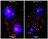 |
Fig. 1. Composite image of the A399-A401 (left) and A21-G114.9 (right) cluster pairs. Optical data are recovered from the DSS, while X-ray data (ASCA for A399-A401, ROSAT for A21-G114.9) are shown in blue, and uGMRT data from this work are overlaid in red. |
2. Observations and data reduction
2.1. uGMRT
Observations of A399-A401 and A21-G114.9 were carried out with the upgraded GMRT (uGMRT) in Band 3 (proposal code: 36_043, P.I.: Bernardi). The total length of the observation was ten hours per pair, including the time spent on calibration sources. Each cluster pair was observed with two distinct pointings, one centred on each galaxy cluster. This results in approximately four hours of on-source time for each target galaxy cluster, and approximately one hour in total spent on calibrators (see Table 2 for observational details).
uGMRT observation details for A399-A401 and A21-G114.9 target cluster pairs.
Data reduction was carried out with the Source Peeling and Atmospheric Modeling (SPAM; Intema 2014) pipeline (as described by Intema et al. 2017). The pipeline started with a pre-processing part that converted the data into a pre-calibrated visibility dataset by performing several rounds of flagging visibilities affected by radio frequency interference (RFI) and then transferring the calibration solutions derived from the primary calibrator to the data. This was followed by direction-independent calibration on the pre-processed visibilities, with several rounds of phase self-calibration, amplitude self-calibration, and more RFI flagging. Finally, from the resulting self-calibration gain table and the final wide-field image, started the direction-dependent (DD) calibration, which determines the DD gain phases from the peeling of the brightest-appearing sources in the field. The gain phases from the peeled sources were spatially fit to constrain a model of the ionosphere, used to predict ionospheric phase delays for arbitrary positions within the field of view. The total bandwidth was reduced at the start of the data calibration with RFI flagging that includes the first and last channels of the band. Then, the remaining wide-band (200 MHz) observations were split into six sub-bands, 33.3 MHz each, and the pipeline ran independently on each sub-band. The calibrated data of each sub-band were then jointly imaged with WSClean v3.1 (Offringa & McKinley 2014). For the A399-A401 pair, the central frequency of the images was 400 MHz. For the A21-G114.9 pair, we excluded the high frequency (467–500 MHz) sub-band, where SPAM could not find enough sources to fit the ionospheric model. This resulted in an image with rms noise five times higher than that of the other sub-bands. After excluding this sub-band, the remaining calibrated data were imaged at the central frequency of 383 MHz.
2.2. Imaging and linear mosaicing
Before imaging, each pointing of the A399-A401 observation was phase-shifted to a common phase centre (RA = 02h58m28s, Dec = +13° 20′18″) and individually deconvolved. We then produced a high-resolution (12″ × 5″, PA 79°) image for each pointing with the same parameters. We adopted a weighting scheme, Briggs robust=0 (Briggs 1995), resulting in an rms noise, σrms ∼ 70 μJy beam−1, similar in both images, which shows a hint of the radio halos’ diffuse emission. The choice of this weighting parameter was motivated by the necessity of recovering the diffuse components of the sources in the field. In order to enhance the sensitivity on Mpc scales, we chose to subtract all compact sources in the field, but, as shown in Fig. 2, we needed to consider also the presence of more extended sources that could contaminate the bridge emission. Thus, we decided to subtract physical scales smaller than 600 kpc: the choice of a 600 kpc scale was a trade-off between the best subtraction of all the compact emission, including the tail of the tailed-radio galaxy in A401 that extends towards the bridge region, and retaining the emission from the radio halos, which extends on scales of approximately 700 kpc. With WSClean, we imaged the field with a uvmin of 464λ to recover only the compact sources, and then subtracted their components from the visibilities. After producing the high-resolution image with the uv-cut, we carefully inspected the model image to ensure that no components of diffuse emission from the bridge area would be subtracted. For each pointing, we then imaged the source-subtracted data with Briggs robust=-0.5 and a Gaussian uv-taper to obtain a 80″ × 80″ resolution image with an rms noise, σrms ∼ 800 μJy beam−1. At this point, we could further enhance the diffuse emission present in each pointing by combining the individual high- and low-resolution images produced with the same parameters into a mosaic. This approach is referred to as linear mosaicing (see, e.g., Holdaway 1999); in other words, the value,  , of a pixel, x, is the average value among all the i pointings, weighted by the primary beam, P:
 (1)
(1)
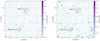 |
Fig. 2. Mosaic radio images at 383 MHz of the A21-G114.9 clusters pair, with overlaid X-ray ROSAT contours. Left panel: high-resolution (15″ × 5″) mosaic image with σrms = 40 μJy beam−1 produced with Briggs robust = 0, showing the compact sources in the field. Right panel: low-resolution (40″ × 40″), compact source-subtracted image with σrms = 230 μJy beam−1. It is generated by Briggs robust=0 and a Gaussian uv-taper. No diffuse emission is revealed. |
Here, the summation, i, is over the pointing centres, xi, Ii(x) is the image produced from the ith pointing, and P(x) is the uGMRT primary beam pattern2. The results of the linear mosaicing procedure are shown in Fig. 3 both for the high- and low-resolution image, with a final rms noise of σrms ∼ 50 μJy beam−1 and σrms ∼ 600 μJy beam−1, respectively.
 |
Fig. 3. Mosaic radio images at 400 MHz of the A399-A401 cluster pair. Left panel: high-resolution (12″ × 5″) mosaic image with σrms = 50 μJy beam−1 produced with Briggs robust = 0 and primary-beam-corrected. A hint of diffuse emission from the radio halos is visible, but no emission is detected in the bridge area. Right panel: low-resolution (80″ × 80″), compact source-subtracted image with σrms = 600 μJy beam−1. It is generated by Briggs robust=-0.5 and a Gaussian uv-taper of 60″. Contour levels start at 2σrms (in green) and increase up to 5σrms (black). The red-dashed box denotes the region where we find a 2σrms detection of a patch of the bridge. The red arrow points to the extension of the A399 radio halo, discussed in Sect. 3.3. |
The same general procedure was followed for the A21-G114.9 observation. Each pointing is shifted to a common phase centre (RA = 00h21m02s, Dec = +28° 22′51″), deconvolved and imaged individually. For each pointing, we produced a high-resolution (15″ × 5″, PA 68°) image with a weighting scheme, Briggs robust=0, and a resulting rms noise, σrms ∼ 50 μJy beam−1. In the high-resolution images there is no evidence of diffuse emission; only compact sources are visible. To investigate the presence of diffuse radio emission corresponding to the SZ detection of the filament reported in Bonjean et al. (2018), we subtracted all compact sources in the field, and then proceeded with low-resolution imaging. For each pointing, we imaged the source-subtracted data with Briggs robust=0, and a Gaussian uv-taper to have a 40″ × 40″ resolution image with an rms noise, σrms ∼ 300 μJy beam−1. In this case, since the diffuse emission is not revealed, we adopted a moderate weighting scheme to have a quality image showing the features in the field. Finally, we combined the high- and low-resolution individual images of each pointing in two final mosaics, following the same approach as that for the A399-A401 pointings. The resulting images with their final rms noise are shown in Fig. 2, where we can notice how there is no visible detection of diffuse emission in the field.
3. Results for the A399-A401 pair
3.1. Limit to the bridge spectral index
The presence of a bridge of low-surface-brightness radio emission is reported in Govoni et al. (2019), where they detected the diffuse emission between the two galaxy clusters at 140 MHz with LOFAR. We are not able to detect the full extension of bridge emission in our 400 MHz uGMRT observations, except for a small patch of emission that we discuss in Sect. 3.3. Through the non-detection we can however place a lower limit on the spectral index of the bridge. The simplest approach would be to use the classical lack-of-detectability criterion, whereby one places a limit at  , where
  is the image rms noise multiplied by the square root of the number of synthesised beams covering bridge area; in this way, we would find a lower limit on the spectral index, α > 3. However, this procedure is only appropriate for point sources, as the noise in interferometric images generally does not simply scale with the area but depends on the baseline distribution, the weighting scheme, and the image fidelity. Therefore, here we followed a similar procedure to the one first introduced in Venturi et al. (2008) for radio halos (see also Kale et al. 2013; Bernardi et al. 2016; Bonafede et al. 2017; Duchesne et al. 2022). In particular, we based our method on the work by Nunhokee et al. (2023) on the A399-A401 pair at 346 MHz, in order to produce comparable results. They found a lower limit for the spectral index, α > 1.5 at a 96% confidence level, and given that our observations were more sensitive than the WSRT and we were still unable to detect the bridge emission, we expected to place an even more stringent constraint.
We refer to this method as “injection”, and a schematic representation of the process is show in Fig. 4. We proceeded as follows:
-
From the model image of the LOFAR detection at 140 MHz, we created a mask by including only the emission from the bridge. This region was selected to include the emission above the 3σ contour in the 80″ resolution LOFAR image, inside a 2 × 3 Mpc box, centred on the bridge (RA = 02h58m26s, Dec = +13° 18′17″, with a position angle of 25° E of the vertical axis), as defined in Govoni et al. (2019). To make sure we were not including the contribution from compact sources in the LOFAR detection, we also masked all sources with emission above the 6σ contour inside the defined box.
-
As mentioned in Sect. 2.1, our data was divided in six sub-bands of 33.3 MHz each, so we needed to extrapolate the bridge model image to each sub-band central frequency, νn = [316, 348, 385, 416, 449, 481] MHz, with
 (2)
(2)where Sn, νn(x, y, α) is the flux density of the model image at the frequency, νn, at the pixels (x, y), S140(x, y) is the flux density of the LOFAR model image, and the spectral index varies between 0 ≤ α ≤ 4 with steps of Δα = 0.25, assuming a uniform spectral index distribution over the source. We discuss the choice of spectral index range in Sect. 3.2.
-
Each extrapolated model image of the bridge was then multiplied with the uGMRT primary beam model to take into account the attenuation of the primary beam in our observation. The final bridge model images were then transformed into visibilities that were injected into our uGMRT source-subtracted, calibrated visibilities of each pointing. We then deconvolved and imaged each pointing separately and linearly combined them, following the same procedure described in Sect. 2.2. In particular, we produced an 80″ resolution mosaic image at the central frequency of 400 MHz for each spectral index, α, with the same parameters used to produce the 80″ image from our observations. An example of such images for different spectral indexes is shown in Fig. 5. As expected, as the spectral index steepens from α = 0 to α = 2.0, the emission of the bridge becomes less and less visible, until it is not detectable above the noise level.
-
We wanted to construct a statistical criterion to determine when the bridge was no longer considered detected; in other words, to determine a lower limit to the spectral index of the bridge. In this sense, the spectral index could be treated as a random variable in the interval 0 ≤ α ≤ 4, even if we sampled it at given values for simplicity. We then defined the ratio, R(α), as
 (3)
(3)where
 defines the flux density of the 400 MHz image with the contribution of the injected visibilities, and S400, is the flux density from the 400 MHz image from the uGMRT observations. Both quantities were measured by summing over the N pixels covering the bridge area (see Fig. 4), masking only the area covered by the small patch of emission (dashed red box in Fig. 3, right panel) that we treated separately in Sect. 3.3. The ratio, R(α), is a decreasing function of α, and has its maximum value when α = 0 and approaches unity for increasing spectral index values, that is, when the bridge spectrum is steeper and the emission is therefore less visible in our injected images. In other words, the ratio, R(α), measures how bright, given a certain spectral index value, α, the injected bridge emission is with respect to the image background. While the definition of R(α) is not the formal definition of a distribution function and does not converge for α → −∞, it does converge when α → ∞. We then normalised the integral of R(α) to unity over the spectral index range, so that R(α) effectively represents a probability to detect a spectral index value given our observations.
 -
We then constructed the cumulative distribution function (
 ) of R(α), defined as
 (4)
(4)The cumulative distribution function of α evaluated at
 gives us the probability of observing an emission with a spectral index,
  in our observations. As shown in Fig. 6, we find that the bridge should be detected in our observations with a probability,
  if
if  . The non-detection in our observations implies that the spectral index of the bridge has a lower limit of αl > 2.2 with a 95% confidence level. It should be noted that the limit value is dependent on the chosen interval range for α, as discussed in Sect. 3.2.
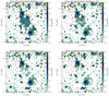 |
Fig. 5. Examples of 400 MHz, uGMRT images where the A399-A401 bridge visibilities were injected, as a function of the spectral index. In particular, we show the different contributions of the bridge when its spectral index steepens, from α = 0 to α = 2.0. In the first two top panels, the bridge is clearly detectable, while approaching the lower limit for the spectral index (left-bottom panel) the emission is less visible, until there is no significant change with respect the image without any injected visibilities. Contour levels are drawn from 2σrms (in green) and increase up to 5σrms (black). A negative contour level at −3σrms is shown in red. |
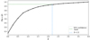 |
Fig. 6. Cumulative distribution function of R(α), normalised to unit area over the interval 0 ≤ α ≤ 4. The horizontal green line marks the 95% probability that the spectral index of the bridge in A399-A401 takes on a value smaller than α ∼ 2.2 (vertical blue line) if the bridge were detected in our uGMRT observations. The non-detection sets a lower limit for the spectral index at αl > 2.2 with a 95% confidence level. |
This result represents an improvement over the constraints from Nunhokee et al. (2023), due to the higher sensitivity of our observations. Our lower limit disfavours the shock re-acceleration processes proposed in Govoni et al. (2019) as the main mechanism responsible for the bridge emission and is consistent with the predictions from Brunetti & Vazza (2020), where the origin of radio bridges is explained by second-order Fermi acceleration of electrons interacting with turbulence on above-Mpc scales, resulting in rather steep spectra.
3.2. The effect of the spectral index range on limit estimates
As presented in Sect. 3.1, we defined the injection procedure to derive the lower limit on the A399-A401 bridge spectral index, by extrapolating the bridge model image from the LOFAR detection to the uGMRT frequency with different spectral index values. We note that the limit value is dependent on the chosen interval range for α, and thus we tested different ranges to investigate the resulting limit. We evaluated the αl value corresponding to the 95% value of the cumulative distribution (as described in the main text, Eq. (4)) as a function of [αmin, αmax], with 0 < αmin < 1 and 2.25 < αmax < 4, in steps of Δα = 0.25 (Fig. 7, left panel). The αmin > 0 boundary is motivated by the fact that an inverted spectral index is not expected for synchrotron emission from a bridge-like source. To investigate the convergence of the cumulative distribution, we defined A as the area under the curve R(α) (Eq. (3)) calculated between αmin and αmax, before normalisation. We then defined the ratio, ϵi:
 (5)
(5)
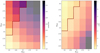 |
Fig. 7. The effect of the spectral index range on the limit result. Left: lower limits at 95% confidence level as a function of spectral index range. The lower and upper bounds of the range can vary between 0 ≤ αmin ≤ 1 and 0 ≤ αmax ≤ 4, respectively. Values above the red line satisfy the criterion of convergence of the cumulative distribution (see right panel). We adopted a lower limit, α > 2.2, obtained using the αmin = 0 ≤ α ≤ 4 = αmax range. Right: convergence of the cumulative probability function with varying spectral index ranges. Values above the red line have ϵ < 1%, which we used as an acceptance criterion (see Eq. (5)). |
where i runs over the number of α steps. For each αmin, ϵi evaluates the percentage difference between the area, Ai, in the interval αmin ≤ α ≤ αmax, i and Ai + 1 in the interval αmin ≤ α ≤ αmax, i + 1, where αmax, i + 1 = αmax, i + 0.25. In other words, when we fixed the value of αmin, we started with the initial area value, Ai, calculated within the interval defined by αmin and αmax, i. Then, we calculated the area value, Ai + 1, within an extended interval that includes αmin and an increased upper bound, αmax, i + 0.25. This allowed us to compare the percentage difference, ϵ, between the area values at each step. We considered the cumulative distribution converging if ϵ < 1%. This was computed for each combination range with 0 ≤ αmin ≤ 1, and 2.25 ≤ αmax ≤ 4. The results are shown in Fig. 7 (right panel), which shows that ϵ decreases with increasing αmax values. This is somewhat expected, as the cumulative distribution function converges for increasing αmax values. We notice that A has the strongest dependence upon αmin, and ϵ changes up to ∼6% across the 0 < αmin < 1 – a small variation anyway. We assumed that estimates of the spectral index lower limit would begin to converge if ϵ < 1%; in other words, if the relative variation between the area under the curve R(α) were smaller than 1% (values above the red line in Fig. 7, left panel). We choose to report the case where the convergence is strongest, with ϵ ∼ 0.5%, leading to α > 2.2 for 0 ≤ α ≤ 4.
3.3. Detection of a patch of bridge emission
As mentioned in Sect. 2.2, we observe a 2σrms level patch of emission in the bridge area in the 80″ resolution image, encompassed by the dashed red box shown in Fig. 3. There were no compact sources in the location corresponding to this region prior to the source subtraction process. Under the assumption that this patch represents a part of the bridge, and that the spectral index is likely variable across the bridge area, this region could present a spectral index flat enough to be detectable in our observations.
Within the 2σrms level contours of the uGMRT image, we measure flux densities of S400 MHz = 8.7 ± 1.7 mJy and S140 MHz = 26.7 ± 3.7 mJy, leading to a spectral index value for the patch of αp = 1.07 ± 0.23.
The uncertainty on the flux density measurements is estimated as
 (6)
(6)
where f = 0.1 is the absolute flux-scale uncertainty (Chandra et al. 2004), Nb the number of beams covering the source, σrms the rms noise sensitivity of the map, and S the measured flux density of the source.
As expected, the spectral index of this emission is significantly flatter than our lower limit, and thus could be revealing a small part of the bridge in our observations.
The interpretation of this 2σrms level patch of emission is not definitive at this time, but it is possible to make some considerations based on the models and detections available in the literature. A physical scenario that could explain the presence of flatter emission patches is one of the predictions from the turbulent re-acceleration model proposed in Brunetti & Vazza (2020). In fact, with their simulations they show how the volume filling factor of the bridge emission should be larger at LOFAR frequencies, resulting in a smoother emission, but at higher frequencies the emission is predicted to be dominated by a clumpy contribution from smaller, more turbulent regions. Moreover, they show that, even during the early stages of a merger between two systems, the dynamics of the collapse can drive weak shocks into the ICM, resulting in an additional compression of the population of turbulent re-accelerated electrons, increasing the radio brightness in these locations.
4. Results for the A21-G114.9 pair
4.1. Injection procedure
In this case, we need to assess how deep our observation should be to detect possible diffuse emission from the filament. This is the first time the A21-G114.9 pair has been observed at radio frequencies, and therefore as opposed to A399-A401 we can only place a limit on the bridge flux density assuming a model for the bridge emission. We defined the morphology and the profile of the mock radio bridge to fit the observations of the most in-depth bridge study Govoni et al. (2019), and to follow the elongated shape of filamentary emission that we would expect from the SZ detection. We detail below the steps we have followed:
-
For the mock bridge brightness profile, we assumed a two-dimensional elliptical Gaussian profile:
![Mathematical equation: $$ \begin{aligned} \begin{array}{ll} I(x,{ y})&\!\!\!= A\exp [(-(a(x-x_{0})^{2}\\&\,\, +2b(x-x_{0})({ y}-{ y}_{0})+c({ y}-{ y}_{0})^2)], \end{array} \end{aligned} $$](/articles/aa/full_html/2024/02/aa46243-23/aa46243-23-eq18.gif) (7)
(7)where
 (8)
(8)and where σ is the Gaussian standard deviation and θ is the rotation angle. The 2D Gaussian model was centred on (x0, y0) = (RA,Dec) = (00h21m02s, +28° 22′51″). The semi-major axis was σy = 12′, the semi-minor axis was σx = 5′, and the ellipse was rotated to θ = 20° W of the vertical axis. We scaled the amplitude, A, so that the integrated flux density of the injected mock bridge varied between 5 mJy and 300 mJy with increasing steps of 5 mJy, and between 300 mJy and 1 Jy with increasing steps of 50 mJy.
-
Each Gaussian model was then multiplied with the uGMRT primary beam model to take into account the attenuation of the primary beam in our observations.
-
The final mock bridge models were transformed into visibilities and injected into our uGMRT source-subtracted calibrated data of each pointing. Then we followed the same procedure described in Sect. 2.2 to produce 40″ resolution mosaic images at the central frequency of 383 MHz for each model flux density, f. Examples of the resulting injected images with different injected flux densities are shown in Fig. 8.
-
We defined the ratio, R(f), as
 (9)
(9)where S383 defines the flux density of the 383 MHz image with no injected visibilities, and
 is the flux density from the 383 MHz image with the contribution of the injected visibilities. Both quantities are measured by summing over the N pixels covering the bridge area within the Gaussian ellipse. The ratio, R(f), is a decreasing function of the injected flux density, f, and hence in the limit, f → ∞ (increasing injected flux), R(f)→0. This implies that there is a value of the injected flux, f, for which the bridge emission should be significantly detected in our 383 MHz observation (i.e.,
  ). Since the bridge is not detected, this sets an upper limit on its flux density at fu.
 -
Following the same procedure of the A399-A401 case, we determined the flux density upper limit by constructing the cumulative distribution function,
 , as defined in Eq. (4)) of R(f), normalised to the unit area over the defined interval for f. As shown in Fig. 9 (left panel), we find that
  for
for  mJy. This means that there is a 95% probability that the bridge emission is lower than 260 mJy, otherwise it would be clearly detected in our uGMRT observations. This sets an upper limit on the bridge flux density at
  mJy with a 95% (∼2σ) confidence level. However, a visual inspection of the image with a 260 mJy injected flux (see Fig. 8) shows that the bridge would be detected at 5σrms. As we were assessing for the first time a procedure to place upper limits on the bridge emission, we evaluated a second criterion for detection, based on the extension and continuity of the injected diffuse emission, as has already been done for radio halos (see, e.g., Bonafede et al. 2017).
 -
We measure
 , the largest detectable size of continuous injected emission above 2σrms, for each image of the injected flux density, f. We consider the bridge to be detected when the emission above 2σrms is continuous for at least the extent of the semi-major axis of the model Gaussian ellipse (
 ). With this criterion, we find that we would consider the bridge to be detected when f ≥ 125 mJy. If we define Atot as the total area of the model Gaussian ellipse over which we performed the injection, the area covered by the emission above 2σrms in the f = 125 mJy image corresponds to the 28% of Atot. This second method sets a lower value for the upper limit,
  mJy. This result is in agreement with the visual inspection of the images, and would be equivalent to the 80% confidence level from the cumulative probability function (see Fig. 9, left panel).
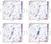 |
Fig. 8. Examples of 383 MHz uGMRT images of A21-G114.9 where the bridge visibilities are injected, as a function-integrated flux density, f. X-ray ROSAT contours are shown in yellow and the location of the X-ray peak is marked with yellow crosses. In particular, we show the different contribution of the injected bridge emission when increasing its flux density, from f = 50 mJy to f = 260 mJy. The visibilities are injected inside a 2D model Gaussian (dashed blue ellipse) with a semi-major axis of 12′ (∼2.5 Mpc) and a semi-minor axis of 5′ (∼500 kpc). We note how in the first two top panels the bridge emission is not significantly detected, while approaching the two values found for the upper limit on the flux density (bottom panels) the emission is continuous and detected over 2σrms. Contour levels are drawn from 2σrms (in purple) to 5σrms (in black). A negative contour level at −3σrms is shown in red. |
This procedure represents the first attempt to adapt to radio bridges the pre-existing injection method introduced in Venturi et al. (2008) for upper limits on radio halos.
These results are dependent on the model we adopted to describe the possible bridge emission. Moreover, given the very few detections of radio bridges so far, the modelling of the morphology and surface brightness of mock emission on such large scales is subject to some arbitrary choices. In comparison with the previous methods, this process presents an improvement by associating a confidence level with the upper limit value, and we are able to compare the results from a second criterion based on the continuity of the recovered emission.
4.2. Fractional recovered flux density
As already noticed when the injection procedure was first introduced for radio halos (Venturi et al. 2008), we expect that the measured flux density of the mock bridge can be different than the injected flux density, as the faintest components may not be found during the imaging process.
As a final consideration, to report the measured value of the flux density upper limit, we evaluated how much of the injected model flux density is effectively recovered in the images we produced. In Fig. 9 (right panel) we plot the fractional recovered flux density with the injected flux density (i.e., the ratio of the measured flux over the injected flux). We can see that the percentage of flux lost in the injection procedure is always smaller than the 23% of the injected flux. In particular, for the upper limits found using the two different methods explained above, we find that the measured value of flux is
 (10)
(10)
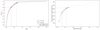 |
Fig. 9. Cumulative distribution function and recovered flux percentage in the injection procedure for A21-G114.9. Left panel: cumulative distribution function of R(f), normalised to unit area over the interval 5 mJy ≤ f ≤ 1 Jy. The horizontal grey line marks the 95% probability that the bridge in A21-G114.9 has a flux density lower than |


as shown in Fig. 9 (right panel) with green and red crosses, respectively. Hence, the resulting upper limits on the measured flux density are
 (11)
(11)
As expected, the loss effect is generally more important at lower flux densities, where the faintest components of the mock bridge on larger scales can result below the noise level. At increasing flux densities, the effect is less severe, and the fractional recovered flux converges around ∼92%.
5. Conclusions
In this work, we analysed uGMRT data of two unique systems of early-stage merging galaxy clusters, where their connection along a filament of the cosmic web is supported by a significant SZ effect detection by the Planck satellite (Bonjean et al. 2018; Planck Collaboration VIII 2013; Planck Collaboration XXII 2016). The A399-A401 pair was already studied with LOFAR, detecting extended diffuse emission in the inter-cluster region (Govoni et al. 2019); the A21-G114.9 pair was unexplored at radio frequencies. Our results can be summarised as follows:
-
For the A399-A401 system we are not able to detect the full extension of the bridge emission in our 400 MHz observations. We followed the injection method (Venturi et al. 2008; Nunhokee et al. 2023) to inject the model visibilities of the detected bridge emission at 140 MHz (Govoni et al. 2019) into our observations, scaling the flux density with different values of spectral indices. We find that the bridge would be detected in our observations if its spectral index were flatter than 2.2 with a 95% confidence level, setting a lower limit at αl > 2.2. This result allows us to test the theoretical models for the bridge origin, disfavouring the shock scenario proposed in Govoni et al. (2019), and is instead consistent with the global predictions of the turbulent (re-)acceleration model of electrons of Brunetti & Vazza (2020).
-
We observed a 2σrms significance patch of emission in the bridge area. Under the assumption that this could represent a part of the bridge emission, for this patch we find a spectral index value of αp = 1.07 ± 0.23, significantly flatter than our limit. This result could indicate a variable spectral index distribution across the bridge area.
-
For the A21-G114.9 system, we do not recover any diffuse emission in our 383 MHz observations. We followed a similar injection procedure, but in this case we placed an upper limit on the flux density of the bridge emission by assuming an elliptical Gaussian model for the description of the mock bridge surface brightness profile. From the injection, we find a flux density upper limit at
 mJy with a 95% confidence level.
 -
We propose a second criterion for placing the upper limit, based on the morphology and continuity of the injected emission recovered in the images. In particular, we consider the bridge detected when the emission is above 2σrms to be continuous for at least the extent of the semi-major axis of the model Gaussian ellipse that defines the injected mock bridge. With this criterion, we find that the upper limit can be placed at
 mJy, in agreement with the visual inspection of the images and equivalent to an 80% confidence level from the cumulative probability function.
 -
We investigated how much of the injected flux is effectively recovered at the end of the injection procedure. We find that the percentage of recovered flux increases with the injected flux and converges around 92%, and with our methodology we consider it unlikely that more than 23% of the injected flux is lost.
The limits that we have derived represent an important constraint on the spectral characterisation of the emission in radio bridges. The large-scale extension, low surface brightness, and steep spectra that we expect from the theoretical models and from the few present observations pose a challenge for multi-frequency detection. However, we have defined in this work a procedure to derive upper limits on their flux density that can be applied to more systems in future observations, which will lead to a more comprehensive view of the radio bridges’ properties and a statistical assessment of their occurrence.
Sν ∝ ν−α.
The uGMRT primary beam shape parameters can be found: http://www.ncra.tifr.res.in/ncra/gmrt/gmrt-users/beam-shape-v1-09sep2022.pdf
Acknowledgments
The authors would like to acknowledge the help and contribution of F. Ubertosi in producing the X-ray images. AB, CJR acknowledge financial support from the ERC Starting Grant ‘DRANOEL’, number 714245.
References
- Akamatsu, H., Fujita, Y., Akahori, T., et al. 2017, A&A, 606, A1 [NASA ADS] [CrossRef] [EDP Sciences] [Google Scholar]
- Bernardi, G., Venturi, T., Cassano, R., et al. 2016, MNRAS, 456, 1259 [NASA ADS] [CrossRef] [Google Scholar]
- Bonafede, A., Cassano, R., Brüggen, M., et al. 2017, MNRAS, 470, 3465 [Google Scholar]
- Bonafede, A., Brunetti, G., Vazza, F., et al. 2021, ApJ, 907, 32 [Google Scholar]
- Bond, J. R., Kofman, L., & Pogosyan, D. 1996, Nature, 380, 603 [NASA ADS] [CrossRef] [Google Scholar]
- Bonjean, V., Aghanim, N., Salomé, P., Douspis, M., & Beelen, A. 2018, A&A, 609, A49 [NASA ADS] [CrossRef] [EDP Sciences] [Google Scholar]
- Botteon, A., van Weeren, R. J., Brunetti, G., et al. 2020, MNRAS, 499, L11 [Google Scholar]
- Briggs, D. S. 1995, PhD Thesis, New Mexico Institute of Mining Technology, USA [Google Scholar]
- Brunetti, G., & Lazarian, A. 2016, MNRAS, 458, 2584 [Google Scholar]
- Brunetti, G., & Vazza, F. 2020, Phys. Rev. Lett., 124, 051101 [Google Scholar]
- Chandra, P., Ray, A., & Bhatnagar, S. 2004, ApJ, 612, 974 [Google Scholar]
- de Jong, J. M. G. H. J., van Weeren, R. J., Botteon, A., et al. 2022, A&A, 668, A107 [NASA ADS] [CrossRef] [EDP Sciences] [Google Scholar]
- Duchesne, S. W., Johnston-Hollitt, M., Riseley, C. J., Bartalucci, I., & Keel, S. R. 2022, MNRAS, 511, 3525 [NASA ADS] [CrossRef] [Google Scholar]
- Fujita, Y., Koyama, K., Tsuru, T., & Matsumoto, H. 1996, PASJ, 48, 191 [NASA ADS] [Google Scholar]
- Fujita, Y., Tawa, N., Hayashida, K., et al. 2008, PASJ, 60, S343 [Google Scholar]
- Govoni, F., Orrù, E., Bonafede, A., et al. 2019, Science, 364, 981 [Google Scholar]
- Hincks, A. D., Radiconi, F., Romero, C., et al. 2022, MNRAS, 510, 3335 [NASA ADS] [CrossRef] [Google Scholar]
- Hoeft, M., & Brüggen, M. 2007, MNRAS, 375, 77 [Google Scholar]
- Hoeft, M., Dumba, C., Drabent, A., et al. 2021, A&A, 654, A68 [NASA ADS] [CrossRef] [EDP Sciences] [Google Scholar]
- Holdaway, M. A. 1999, in Synthesis Imaging in Radio Astronomy II, eds. G. B. Taylor, C. L. Carilli, & R. A. Perley, ASP Conf. Ser., 180, 401 [NASA ADS] [Google Scholar]
- Intema, H. T. 2014, Astrophysics Source Code Library [record ascl:1408.006] [Google Scholar]
- Intema, H. T., Jagannathan, P., Mooley, K. P., & Frail, D. A. 2017, A&A, 598, A78 [NASA ADS] [CrossRef] [EDP Sciences] [Google Scholar]
- Kale, R., Venturi, T., Giacintucci, S., et al. 2013, A&A, 557, A99 [NASA ADS] [CrossRef] [EDP Sciences] [Google Scholar]
- Murgia, M., Govoni, F., Feretti, L., & Giovannini, G. 2010, A&A, 509, A86 [NASA ADS] [CrossRef] [EDP Sciences] [Google Scholar]
- Nunhokee, C. D., Bernardi, G., Manti, S., et al. 2023, MNRAS [Google Scholar]
- Oegerle, W. R., & Hill, J. M. 2001, AJ, 122, 2858 [NASA ADS] [CrossRef] [Google Scholar]
- Offringa, A. R., McKinley, B., Hurley-Walker, N., et al. 2014, MNRAS, 444, 606 [Google Scholar]
- Pfrommer, C., & Enßlin, T. A. 2004, A&A, 413, 17 [NASA ADS] [CrossRef] [EDP Sciences] [Google Scholar]
- Planck Collaboration VIII. 2013, A&A, 550, A134 [NASA ADS] [CrossRef] [EDP Sciences] [Google Scholar]
- Planck Collaboration XXII. 2016, A&A, 594, A22 [NASA ADS] [CrossRef] [EDP Sciences] [Google Scholar]
- Radiconi, F., Vacca, V., Battistelli, E., et al. 2022, MNRAS, 517, 5232 [NASA ADS] [CrossRef] [Google Scholar]
- van Weeren, R. J., de Gasperin, F., Akamatsu, H., et al. 2019, Space Sci. Rev., 215, 16 [Google Scholar]
- Vazza, F., Ettori, S., Roncarelli, M., et al. 2019, A&A, 627, A5 [NASA ADS] [CrossRef] [EDP Sciences] [Google Scholar]
- Venturi, T., Giacintucci, S., Dallacasa, D., et al. 2008, A&A, 484, 327 [NASA ADS] [CrossRef] [EDP Sciences] [Google Scholar]
- Venturi, T., Giacintucci, S., Merluzzi, P., et al. 2022, A&A, 660, A81 [NASA ADS] [CrossRef] [EDP Sciences] [Google Scholar]
- Vernstrom, T., Heald, G., Vazza, F., et al. 2021, MNRAS, 505, 4178 [NASA ADS] [CrossRef] [Google Scholar]
- Vikhlinin, A., Burenin, R. A., Ebeling, H., et al. 2009, ApJ, 692, 1033 [Google Scholar]
- ZuHone, J. A., Markevitch, M., Brunetti, G., & Giacintucci, S. 2013, ApJ, 762, 78 [Google Scholar]
All Tables
Position, redshift, and mass of the two pairs of target galaxy clusters analysed in this work.
All Figures
|
Fig. 1. Composite image of the A399-A401 (left) and A21-G114.9 (right) cluster pairs. Optical data are recovered from the DSS, while X-ray data (ASCA for A399-A401, ROSAT for A21-G114.9) are shown in blue, and uGMRT data from this work are overlaid in red. |
| In the text | |
|
Fig. 2. Mosaic radio images at 383 MHz of the A21-G114.9 clusters pair, with overlaid X-ray ROSAT contours. Left panel: high-resolution (15″ × 5″) mosaic image with σrms = 40 μJy beam−1 produced with Briggs robust = 0, showing the compact sources in the field. Right panel: low-resolution (40″ × 40″), compact source-subtracted image with σrms = 230 μJy beam−1. It is generated by Briggs robust=0 and a Gaussian uv-taper. No diffuse emission is revealed. |
| In the text | |
|
Fig. 3. Mosaic radio images at 400 MHz of the A399-A401 cluster pair. Left panel: high-resolution (12″ × 5″) mosaic image with σrms = 50 μJy beam−1 produced with Briggs robust = 0 and primary-beam-corrected. A hint of diffuse emission from the radio halos is visible, but no emission is detected in the bridge area. Right panel: low-resolution (80″ × 80″), compact source-subtracted image with σrms = 600 μJy beam−1. It is generated by Briggs robust=-0.5 and a Gaussian uv-taper of 60″. Contour levels start at 2σrms (in green) and increase up to 5σrms (black). The red-dashed box denotes the region where we find a 2σrms detection of a patch of the bridge. The red arrow points to the extension of the A399 radio halo, discussed in Sect. 3.3. |
| In the text | |
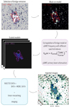 |
Fig. 4. Schematic flowchart of the injection method, described in Sect. 3.1. |
| In the text | |
|
Fig. 5. Examples of 400 MHz, uGMRT images where the A399-A401 bridge visibilities were injected, as a function of the spectral index. In particular, we show the different contributions of the bridge when its spectral index steepens, from α = 0 to α = 2.0. In the first two top panels, the bridge is clearly detectable, while approaching the lower limit for the spectral index (left-bottom panel) the emission is less visible, until there is no significant change with respect the image without any injected visibilities. Contour levels are drawn from 2σrms (in green) and increase up to 5σrms (black). A negative contour level at −3σrms is shown in red. |
| In the text | |
|
Fig. 6. Cumulative distribution function of R(α), normalised to unit area over the interval 0 ≤ α ≤ 4. The horizontal green line marks the 95% probability that the spectral index of the bridge in A399-A401 takes on a value smaller than α ∼ 2.2 (vertical blue line) if the bridge were detected in our uGMRT observations. The non-detection sets a lower limit for the spectral index at αl > 2.2 with a 95% confidence level. |
| In the text | |
|
Fig. 7. The effect of the spectral index range on the limit result. Left: lower limits at 95% confidence level as a function of spectral index range. The lower and upper bounds of the range can vary between 0 ≤ αmin ≤ 1 and 0 ≤ αmax ≤ 4, respectively. Values above the red line satisfy the criterion of convergence of the cumulative distribution (see right panel). We adopted a lower limit, α > 2.2, obtained using the αmin = 0 ≤ α ≤ 4 = αmax range. Right: convergence of the cumulative probability function with varying spectral index ranges. Values above the red line have ϵ < 1%, which we used as an acceptance criterion (see Eq. (5)). |
| In the text | |
|
Fig. 8. Examples of 383 MHz uGMRT images of A21-G114.9 where the bridge visibilities are injected, as a function-integrated flux density, f. X-ray ROSAT contours are shown in yellow and the location of the X-ray peak is marked with yellow crosses. In particular, we show the different contribution of the injected bridge emission when increasing its flux density, from f = 50 mJy to f = 260 mJy. The visibilities are injected inside a 2D model Gaussian (dashed blue ellipse) with a semi-major axis of 12′ (∼2.5 Mpc) and a semi-minor axis of 5′ (∼500 kpc). We note how in the first two top panels the bridge emission is not significantly detected, while approaching the two values found for the upper limit on the flux density (bottom panels) the emission is continuous and detected over 2σrms. Contour levels are drawn from 2σrms (in purple) to 5σrms (in black). A negative contour level at −3σrms is shown in red. |
| In the text | |
|
Fig. 9. Cumulative distribution function and recovered flux percentage in the injection procedure for A21-G114.9. Left panel: cumulative distribution function of R(f), normalised to unit area over the interval 5 mJy ≤ f ≤ 1 Jy. The horizontal grey line marks the 95% probability that the bridge in A21-G114.9 has a flux density lower than |
| In the text | |
Current usage metrics show cumulative count of Article Views (full-text article views including HTML views, PDF and ePub downloads, according to the available data) and Abstracts Views on Vision4Press platform.
Data correspond to usage on the plateform after 2015. The current usage metrics is available 48-96 hours after online publication and is updated daily on week days.
Initial download of the metrics may take a while.