| Issue |
A&A
Volume 667, November 2022
|
|
|---|---|---|
| Article Number | A5 | |
| Number of page(s) | 23 | |
| Section | Extragalactic astronomy | |
| DOI | https://doi.org/10.1051/0004-6361/202243582 | |
| Published online | 31 October 2022 | |
Dynamical characterization of galaxies up to z ∼ 7⋆
1
Cosmic Dawn Center (DAWN), Copenhagen N, Denmark
e-mail: This email address is being protected from spambots. You need JavaScript enabled to view it.
2
Niels Bohr Institute, University of Copenhagen, Jagtvej 128, 2200 Copenhagen N, Denmark
3
Scuola Normale Superiore, Piazza dei Cavalieri 7, 56126 Pisa, Italy
4
Istituto Nazionale di Astrofisica, Vicolo dell’Osservatorio 5, 35122 Padova, Italy
Received:
18
March
2022
Accepted:
12
August
2022
Abstract
Context. The characterization of the dynamical state of galaxies up to z ∼ 7 is crucial for constraining the mechanisms that drive the mass assembly in the early Universe. However, it is unclear whether the data quality of typical observations obtained with current and future facilities is sufficient to perform a solid dynamical analysis at these redshifts.
Aims. This paper defines the angular resolution and signal-to-noise ratio (S/N) required for a robust characterization of the dynamical state of galaxies up to the Epoch of Reionization. The final aim is to help design future spatially resolved surveys targeting emission lines of primeval galaxies.
Methods. We investigate the [C II]-158 μm emission from six z ∼ 6 − 7 Lyman break galaxies at three different inclinations from the SERRA zoom-in cosmological simulation suite. The SERRA galaxies cover a range of dynamical states: from isolated disks to major mergers. We create 102 mock observations with various data quality and apply the kinematic classification methods commonly used in the literature. These tests allow us to quantify the performances of the classification methods as a function of angular resolution and S/N.
Results. We find that barely resolved observations, typical of line detection surveys, do not allow the correct characterization of the dynamical stage of a galaxy, resulting in the misclassification of disks and mergers in our sample by 100 and 50%, respectively. However, even when using spatially resolved observations with data quality typical of high-z galaxies (S/N ∼ 10, and ∼3 independent resolution elements along the major axis), the success rates in the merger identification of the standard kinematic classification methods, based on the analysis of the moment maps, range between 50 and 70%. The high angular resolution and S/N needed to correctly classify disks with these standard methods can only be achieved with current instrumentation for a select number of bright galaxies. We propose a new classification method, called PVsplit, that quantifies the asymmetries and morphological features in position-velocity diagrams using three empirical parameters. We test PVsplit on mock data created from SERRA galaxies, and show that PVsplit can predict whether a galaxy is a disk or a merger provided that S/N ≳ 10, and the major axis is covered by ≳3 independent resolution elements.
Key words: galaxies: high-redshift / galaxies: kinematics and dynamics / galaxies: interactions / galaxies: ISM
Movie associated to Fig. 17 is available at https://www.aanda.org
© F. Rizzo et al. 2022
 Open Access article, published by EDP Sciences, under the terms of the Creative Commons Attribution License (https://creativecommons.org/licenses/by/4.0), which permits unrestricted use, distribution, and reproduction in any medium, provided the original work is properly cited.
This article is published in open access under the Subscribe-to-Open model. This email address is being protected from spambots. You need JavaScript enabled to view it. to support open access publication.
1. Introduction
In the current paradigm of cosmological structure formation, the evolution of galaxies results from the interplay between different processes: accretion of cold gas, minor and major mergers, stellar and active-galactic-nuclei feedback (e.g., Somerville & Davé 2015; Cimatti et al. 2019). Some of these processes (e.g., gas accretion) lead to the formation of a disk structure (e.g., Dekel et al. 2009; Pallottini et al. 2017b; Kohandel et al. 2019; Kretschmer et al. 2021; Tamfal et al. 2022) or the increase of the gas turbulence within early galaxies (e.g., stellar feedback, minor mergers, Ceverino et al. 2015; Danovich et al. 2015; Pillepich et al. 2019; Kohandel et al. 2020; Kretschmer et al. 2021). On the contrary, frequent major merger events or counter-rotating gas streams can be potentially disruptive, destroying and preventing the rebuilding of the disks on timescales comparable or longer than the dynamical times of the galaxy (e.g., Bournaud et al. 2007; Dubois et al. 2012; Zolotov et al. 2015; Dekel et al. 2020). Studying the dynamics of star-forming galaxies across cosmic time is crucial to constrain the relative importance of processes mostly contributing to the growth of galaxies and the evolution of their morphology (e.g., Wisnioski et al. 2015, 2019; Turner et al. 2017; Johnson et al. 2018; Krumholz et al. 2018; Kohandel et al. 2020; Ejdetjärn et al. 2022; Romano et al. 2021).
The prevalence of rotating disks among star-forming galaxies at z ∼ 1–3 has supported the idea that, during this epoch, galaxies mainly grow in mass due to smooth accretion of cold gas inflowing through the cosmic web (i.e., secular growth), while mergers seem to play only a minor role (Wisnioski et al. 2015). However, the fraction of rotating disks at these intermediate redshifts has been debated in the last years. At z ∼ 1, the fraction of disks in the star-forming galaxy population goes from 80% (Wisnioski et al. 2015, 2019) to 42% (Rodrigues et al. 2017) depending on the criteria employed for the classification. Simons et al. (2019) show that the angular resolutions of current near-infrared integral-field-unit (IFU) observations hampered the possibility to robustly distinguish the regular rotation of a disk from the orbital motions of interacting galaxies. By analyzing synthetic IFU observations of simulated galaxies at z ∼ 2, Simons et al. (2019) conclude that the probability that a merger is classified as a disk could be as high as 100% for close-pair merging galaxies.
The characterization of the dynamics of galaxies just after (4 ≲ z ≲ 6) and within the Epoch of Reionization (z ≳ 6) is still in its infancy as spatially resolved observations targeting emission lines are available only for about ten of sub-mm sources (e.g., Rizzo et al. 2020; Lelli et al. 2021; Rizzo et al. 2021) and a handful of Lyman break galaxies (e.g., Jones et al. 2017; Fujimoto et al. 2021). Instead, the number of marginally resolved observations aiming at inferring the integrated properties of early galaxies has increased in the last five years (Smit et al. 2018; Le Fèvre et al. 2020; Bouwens et al. 2022). In their pioneering work, Smit et al. (2018) used marginally resolved Atacama Large Millimeter/Submillimetre Array (ALMA, Wootten & Thompson 2009) observations of the [C II]-158 μm emission line to show that two star-forming galaxies at z ∼ 7 have smooth velocity gradients and interpreted them as being rotationally supported disks. Similar results are obtained in studies of individual galaxies at z ∼ 6–8 (Bakx et al. 2020; Harikane et al. 2020). However, given the low angular resolution of these data, they can not rule out the possibility that one or more merging [C II]-bright satellites are mimicking the smooth gradient observed in the velocity maps (see discussion in Smit et al. 2018; Simons et al. 2019). Instead, a gradient in the velocity fields of two Lyman break galaxies at z = 6.1 and 7.1, combined with the identification of two compact components, has been interpreted as evidence of mergers (Jones et al. 2017; Hashimoto et al. 2019). Recently, Le Fèvre et al. (2020) and Romano et al. (2021) performed the first systematic morpho-kinematic analysis of a statistically significant sample of z ∼ 4–6 main-sequence galaxies from the ALMA Large Program to INvestigate [C II] at Early times (ALPINE) survey. After combining the morphological and kinematic analysis of the [C II] observations with the rest-frame UV and optical data, Romano et al. (2021) conclude that 23 out of the 75 ALPINE galaxies are merging systems. This large fraction of mergers in the ALPINE sample could imply a significant contribution of major mergers to the mass assembly in the early Universe (Le Fèvre et al. 2020; Romano et al. 2021), confirming previous results based on the count of close-pair galaxies in photometric surveys (Mantha et al. 2018; Duncan et al. 2019). However, due to the sensitivity and angular resolutions of the ALPINE observations, the kinematic characterization and, consequently, the merger fraction may be uncertain.
To summarize, both at intermediate and high-z, characterizing the kinematic state of galaxies has been challenging (e.g., Gonçalves et al. 2010; Smit et al. 2018; Simons et al. 2019) since the classification techniques used in the literature (e.g., Shapiro et al. 2008; Bellocchi et al. 2012; Wisnioski et al. 2015, 2019) have focused on the analysis of the kinematic maps (velocity and velocity-dispersion fields). At the typical angular resolution of current observations, any irregularities and disturbances in the kinematic maps of distant galaxies are usually smoothed out so that galaxies appear more regular than they are (e.g., Bellocchi et al. 2012; Simons et al. 2019). Further, kinematic maps cannot be considered a thorough representation of the data in their native three-dimensional space (RA, Dec, Frequency) since they are obtained after masking the low signal-to-noise (S/N) regions and integrating them along the spectral axis. In addition, most of the kinematic classification techniques have been tested and calibrated on IFU observations of intermediate-z galaxies (e.g., Shapiro et al. 2008; Bellocchi et al. 2012; Wisnioski et al. 2015; Simons et al. 2019). Unlike interferometric data, IFU observations are characterized by both a limited range of angular resolutions and spectral resolutions that are typically a factor of ≳3 worse than those achievable with ALMA. A quantitative investigation of their range of applicability to interferometric observations with a wide range of S/N ratios and angular resolutions is still missing (e.g., see also discussion in Glazebrook 2013).
With this work, we aim to fill this gap by quantifying how the data quality affects the correct characterization of the dynamical stage of high-z galaxies observed with ALMA. The results of this paper will help to design future surveys aimed at constraining the dynamical properties of galaxies up to the Epoch of Reionization (EoR). To this end, we generate mock ALMA observations (Kohandel et al. 2020) by using simulated galaxies from the SERRA suite at z ∼ 6–7 (Pallottini et al. 2022). After analyzing the mock data sets as we would analyze real data, we discuss the potential biases of the typical kinematic classification methods as a function of the angular resolutions and the S/N ratios of the observations. In this first paper, we also present and discuss a new technique aiming at distinguishing different dynamical states of galaxies even at low-angular resolutions. Detailed analysis of a representative sample of galaxies will be presented in the second paper of this series.
This paper is organized as follows: we summarize the main characteristics of the zoom-in cosmological simulations adopted in this work and the galaxies selected for our analysis in Sects. 2 and 3. In Sects. 4 and 5, we describe how we created the mock data and extracted the kinematic properties. The application of the standard kinematic classification techniques is presented and discussed in Sect. 6. In Sect. 7, we introduce a new proxy for characterizing different dynamical states of galaxies using medium and low-angular resolution observations. Finally, we summarize the results in Sect. 8.
2. Numerical simulations
SERRA is a suite of simulations that focuses on zooming in on the formation and evolution of galaxies in the EoR (see Pallottini et al. 2022, for details). Gas and dark matter are evolved with a customized version of adaptive mesh refinement code RAMSES (Teyssier 2002). Adopting KROME (Grassi et al. 2014), SERRA includes non-equilibrium chemical (and thermal) evolution up to the formation of H2 (Pallottini et al. 2017a). The chemical network used in SERRA includes H, He, H+, H−, He, He+, He++, H2,  and electrons (Bovino et al. 2016). Metals and dust contribute to the cooling of the gas and H2 formation. Metallicity is tracked as the sum of heavy elements, assuming solar abundance ratios of different metal species (Asplund et al. 2009). Dust formation and evolution are not tracked explicitly: it is assumed that the dust-to-gas mass ratio scales with metallicity, and an MW-like grain size distribution is adopted.
Molecular hydrogen is converted into stars following a Kennicutt-Schmidt-like relation (Schmidt 1959; Kennicutt 1998). Stars in SERRA affect the chemical and energy budget of the interstellar medium (ISM) via feedback processes that include Type II and Ia Supernovæ, winds from OB and AGB stars, and radiation pressure, which give both a thermal and turbulent energy contribution to the ISM (Agertz et al. 2013; Pallottini et al. 2017b). In particular, input energy is computed from stellar evolutionary tracks (Leitherer et al. 1999) adopting PADOVA stellar populations (Bertelli et al. 1994) and a Kroupa (2001) initial mass function. Feedback processes inject a fraction of the energy as a thermal contribution and a part as turbulent (kinetic) contribution. The former can cool according to the KROME thermo-chemical evolution, the latter dissipates (Teyssier et al. 2013) on a eddy turn-over timescale (Mac Low 1999). The injected fractions depend on the process and the environment (see Appendix A in Pallottini et al. 2017b), e.g., SNs exploding in a low density medium are in a Sedov-Taylor phase, thus resulting in a ≃70% and ≃30% contribution to the thermal and turbulent energy. Further, stars contribute to the interstellar radiation field (ISRF), which is tracked on the fly using the radiative transfer module RAMSES-RT (Rosdahl et al. 2013), which is consistently coupled to the chemical evolution of the gas (Pallottini et al. 2019; Decataldo et al. 2019).
In the SERRA suite, simulations evolve from cosmological initial conditions, computed with MUSIC (Hahn & Abel 2011) at z = 100. In each simulation the comoving volume is (20 Mpc/h)3 and its evolution is followed down to z = 6. For each independent volume, the simulation zoom-in on the formation and evolution of ∼10 − 20 galaxies, whose ISM is resolved on scales of ≃1.2 × 10⁴ M⊙, ≃ 30 pc, i.e. masses and sizes typical of Molecular Clouds (e.g., Federrath & Klessen 2013). Currently, at z ≃ 6 − 7 the SERRA suite has a total of ≃200 galaxies with mass range ∼ 108 − 1010 M⊙ (Pallottini et al. 2022). As shown in Pallottini et al. (2022), SERRA galaxies have a specific SFR that ranges from sSFR ∼ 100 Gyr−1 for young (t⋆ ≲ 100 Myr), small galaxies (M⋆ ≲ 108 M⊙) to sSFR ∼ 10 Gyr−1 for older (t⋆ ≳ 200 Myr) more massive ones (M⋆ ≳ 109 M⊙), in good agreement with high-z data (Jiang et al. 2013; Rinaldi et al. 2022). In Fig. 1 (left panel), we show the SFR – M⋆ distribution for SERRA galaxies at z = 6 − 7.2 (Kohandel et al., in prep.). The size-stellar mass relation from SERRA has the same slope as the one observed in the local Universe (Brodie et al. 2011; Norris et al. 2014), but it is downshifted by about one order of magnitude because of redshift evolution (Shibuya et al. 2015) and it is broadly consistent with lensed galaxies observed at high-z (Bouwens et al. 2021; Vanzella et al. 2019). In Fig. 1 (central panel), we show the stellar effective radii as a function of stellar mass for the SERRA galaxies at z = 6 − 7.2. The effective radii span a range from 0.05 to 0.8 kpc. For dark-matter halos with masses Mh ≳ 5 × 10¹⁰ M⊙, the SERRA stellar-to-halo mass relation is consistent with abundance matching works (Behroozi et al. 2013) and state-of-art zoom-in simulation suites (Ceverino et al. 2017; Ma et al. 2018) (for lower masses, see the discussion on the effect of photodissociation on the relation in Pallottini et al. 2022).
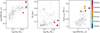 |
Fig. 1. Physical properties of the parent and selected sample. The gray stars show the position of EoR galaxies from the SERRA suite (see Pallottini et al. 2022; Kohandel et al., in prep.) in the SFR-M⋆ (left panel), size-M⋆ (medium panel), L[CII]-SFR (right panel) planes. The squares and circles show the selected disks and mergers, respectively, color-coded with the names as indicated by the color-bar. The green diamond shows the disturbed disk Freesia. |
Individual ion abundances (such as C+) and line emissions (such as [C II]) are recomputed in post-processing by using the spectral synthesis code CLOUDY (Ferland et al. 2017). The [C II] emission line is known to originate from all the gas phases of the ISM, albeit predominantly from cold neutral and molecular gas in the so-called photodissociation regions (see Wolfire et al. 2022, for a recent review), thus is a unique tracer of galaxy kinematics probing out to large galactocentric radii. In SERRA the internal structure of molecular clouds is not resolved; thus, an additional model is adopted to account for the turbulent and clumpy structure of the ISM (see Vallini et al. 2018; Pallottini et al. 2019, for details). Further modeling is performed to bridge the outputs of zoom-in simulations and 3D observations by generating Hyper-spectral Data Cubes (HDC) for each given emission line (see Kohandel et al. 2020, for the details). To summarize, we compute [C II] luminosity on a cell by cell basis depending on gas density, metallicity, thermal+turbulent broadening, column density, and ISRF intensity. The distribution of the total [C II] luminosity (L[CII]) as a function of SFR is shown in Fig. 1 for the z = 6 − 7.2 SERRA galaxies. Given the gas position, line of sight velocity, and thermal+turbulent broadening, we construct HDCs with two spatial and one spectral dimension. Such data products are especially handy for galaxy kinematic studies and can be used for direct comparison of the simulations and spatially resolved galaxy observations.
In this work, we select cubic regions centered on chosen galaxies with a fixed inclination adopting a side-length of 8 kpc and mapping the volume to [C II] emission HDCs with 2563 voxels, i.e. a setup similar to Kohandel et al. (2020). Thus, our HDCs have a spectral resolution of ≃ 3.1 km s−1 and a spatial resolution of ≃ 31.2 pc, corresponding to an angular resolution of 0.005″ at z = 6.
3. Sample selection
Our sample contains six galaxies in the redshift range 6 ≲ z ≲ 7 from the SERRA suite. We selected three rotating disks (Lantana, Opuntia and Petunia), one disturbed disk (Freesia) and two major mergers. (Adenia and Fuchsia). Similarly to Kohandel et al. (2019), the dynamical stages of these galaxies are identified based on the morphology of the [C II] line surface brightness maps and the corresponding spectra extracted for their face-on1 and edge-on views. The three disk galaxies meet the following two criteria: there are no galaxies (M⋆ ≳ 106 M⊙, i.e. more than about 100 stellar particles) identified within ≃ 4 kpc at the selected redshift and in the past ≃15 Myr. The two merger systems are characterized by two companions separated by a distance ≲0.8 kpc and a mass ratio > 0.4. The disturbed disk Freesia has some disturbances driven by the close encounter with a giant clump of gas (see details in Kohandel et al. 2020).
To support the visual identification, we computed the circularity of the gas disk, using a method similar to the one adopted in Simons et al. (2019). As done in Zana et al. (2022), we identified the center of the galaxy with the minimum of the gravitational potential, that is computed with the Grudić & Gurvich (2021) implementation of the Barnes & Hut (1986) algorithm. We then iteratively fitted a cold (T ≤ 1.5 × 10³ K) gas disk, defined in terms of its angular momentum (Ld), radius and size, similarly to what is described in Mandelker et al. (2014). The circularity is defined by averaging the specific angular momentum J along the direction defined by the disk (Ld/|Ld|) and normalized by  . In a disk, the gas motion is aligned with the net galaxy rotation resulting in a circularity close to 1.
The gas of the selected disk galaxies (Opuntia, Lantana, and Petunia) have high circularity (0.49, 0.96, and 0.82, respectively) and the angular momenta of gas and stars have misalignments ≲20 deg. The disturbed disk (Freesia) has a high circularity of 0.77, but the fitted disk size is 1.12 kpc, i.e. the distance between the main galaxy and its satellite. Instead, the mergers (Adenia, Fuchsia) have lower circularities (0.23, 0.44) and, further, have strong misalignments between the gas and stellar angular momenta (113, 42 deg).
In Fig. 1, the position of galaxies in our sample is shown on the SFR-M⋆, size-M⋆, L[CII]-SFR planes with respect to the parent sample of EoR galaxies from SERRA. Galaxies in our sample span a stellar mass range M⋆ ∼ (0.3 − 1.7)×1010 M⊙, a star-formation rate SFR ∼ 20 − 100 M⊙ yr−1, resulting in a specific star formation rate 1.6 Gyr−1 ≤ sSFR ≡ SFR/M⋆ ≤ 8 Gyr−1 with Opuntia having the lowest value and Fuchsia having the highest value. The sizes of the selected galaxies are typical of the parent sample, with Freesia being the more extended one (i.e. R∗ ≃ 0.7 kpc). The L[CII] range from 0.6 to 6.3 ×10⁸ L⊙, typical of galaxies with [C II] detection at z ≳ 6 (e.g., Carniani et al. 2020; Sommovigo et al. 2022). In Table 1, we report the general properties of the selected SERRA galaxies. For each galaxy, HDCs are generated using three inclination angles (30, 60, and 80 deg). To have a visual overview, in Fig. 2, the stellar surface density (Σ⋆) and [C II] line surface brightness (Σ[CII]) maps for the inclination angle of 60 deg of our sample are plotted.
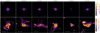 |
Fig. 2. Sample of SERRA galaxies adopted in this work. For each galaxy we plot the stellar surface density (Σ⋆, upper panels) and the [C II] line surface brightness (Σ[CII], lower panels) for an inclination of 60 degrees. The field of view has a size of 8 kpc. See Table 1 for the main properties of the galaxies. |
Properties of SERRA galaxies analyzed in this work.
4. Mock observations
To study how the data quality (angular resolution and S/N) impacts the classification of disks and mergers, we generated 102 mock observations from the simulated [C II] emission HDCs of galaxies described in Sect. 3. We rebin the HDC to have data cubes with spectral channels of width 30 km s−1, as typically done for observations of galaxies at z ≳ 4 (e.g., Lelli et al. 2021; Rizzo et al. 2021). This spectral resolution allows us to recover the velocity dispersion of SERRA galaxies with typical values ≳30 km s−1 (Kohandel et al. 2020). Based on the data quality, we divided the synthetic observations into the following five categories (see Table 2):
-
a)
Ideal data: ideal observations at high angular resolution and very high S/N. These mock data are obtained after convolving the cubes with a Gaussian point-spread-function with a full width at half maximum (FWHM) of 0.02″ (≃ 120 pc). Then, we added Gaussian noise to each pixel to reach an S/N ratio of ∼402.
-
b)
ALMA high-angular resolution, high S/N data: We used the tasks SIMOBSERVE in the CASA package (McMullin et al. 2007) to create ALMA interferometric observations at the nominal angular resolution of 0.02″ (≃ 120 pc) and with a S/N ratio of 10. The galaxies are then imaged with a natural weighting of the visibilities using the task SIMANALYZE. On average, the area of the galaxies with [C II] surface brightness larger than 3 times the rms noise (3 rms) is covered by ≈10 resolution elements in each spectral channel.
-
c)
ALMA medium- and low-angular resolution, high S/N data: Similar to point b), but with nominal angular resolutions of 0.05″ (≃ 0.3 kpc) and 0.1″ (≃ 0.6 kpc). The area of the galaxies at ≳3 rms is covered on average by 3 and 2 resolution elements per spectral channel for the medium and low-resolution data, respectively.
-
d)
ALMA high- and medium-angular resolution, low S/N data: We created ALMA mock data using the same methodology described at point b) but with an S/N of ∼5. In this case, the area of the galaxies with [C II] surface brightness ≳3 rms is covered by ≈4 and 2 resolution elements in each spectral channel for the high and medium-resolution data, respectively. We decided to create this dataset for the galaxies at 60 deg as it is the most probable inclination of observed galaxies (Romanowsky & Fall 2012). Our conclusions about the impact of S/N on the kinematic classification do not change as a function of inclination.
-
e)
ALMA barely resolved, low S/N data: We used SIMOBSERVE and SIMANALYZE to create mock data matching the data quality of the ALPINE sample as well as most observations of z ≳ 4 galaxies (e.g., Le Fèvre et al. 2020; Smit et al. 2018; Bakx et al. 2020). On average, the ratios between the deconvolved [C II] effective radius and the beam size range between 0.3 (e.g., ALPINE sample Le Fèvre et al. 2020; Fujimoto et al. 2020) and 0.5 (e.g., Smit et al. 2018; Bakx et al. 2020). The CII emitting gas in SERRA galaxies described in Sect. 3 has an average effective radius of ∼0.07″. For this dataset a resolution of 0.15″ (≃ 0.9 kpc) allowed us to reproduce the typical angular resolutions of current z ≳ 4 observations. The barely resolved ALMA data have an S/N ratio of ∼4 that corresponds to S/N ratios in the range 6–10 in the moment-0 maps, comparable with the values reported in Béthermin et al. (2020) and Fujimoto et al. (2020) for the ALPINE galaxies. On average, the area of the galaxies with [C II] surface brightness ≳3 rms is covered by ≈0.3 resolution elements in each spectral channels.
Figures 3 and 4 show the moment-0 ([C II] integrated across the spectral axis), moment-1 (flux-weighted velocity), and moment-2 (flux-weighted velocity dispersion) maps obtained from the mock data a) – d) for two representative galaxies, the disk Petunia and the merger Adenia at i = 60 deg. We note that currently only a handful of observations of lensed and non-lensed dusty star-forming galaxies at z ≳ 4 have data quality comparable to that described at points b)-d) (e.g., Neeleman et al. 2020; Rizzo et al. 2020, 2021; Fraternali et al. 2021; Lelli et al. 2021). Most observations of main-sequence galaxies at z ≳ 4 (e.g., Le Fèvre et al. 2020; Smit et al. 2018; Bakx et al. 2020) have been designed, instead, for line detection, and therefore their data quality is comparable to the 18 mock data described at point e). A test for this low-resolution and low-S/N data is discussed in Sect. 6.3. However, for the rest of the paper, we adopt the 84 synthetic observations described at points a)–d), if not otherwise stated, as in the near future, medium- and low-angular resolution, high S/N ALMA, and JWST observations will be available for tens z ≳ 4 galaxies.
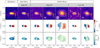 |
Fig. 3. Moment-0 (upper panels), 1 (medium panels), and 2 (bottom panels) for the disk Petunia at 60 deg obtained from the simulated cube (Col. 1) and the mock cubes described at points a) – d) in Sect. 4 (Cols. 2–7) at different angular resolutions (the beam is shown in the bottom left corner as the gray ellipse). In the mock moment-0 maps, the white contours are at 2 and 10 times the rms noise and the color bars are in units of 10 mJy pixel−1 km s−1 in the first column and 100 mJy beam−1 km s−1 for the mock observations. |
5. Kinematic modeling
5.1. Data analysis
We assumed that the [C II] emitting gas moves in circular orbits to extract the kinematic properties of galaxies in our sample. Deviations from pure circular orbits include radial and vertical motions due to outflows and inflows or asymmetry of the galactic gravitational potential driven by mergers, bars, or spiral arms (e.g., Fraternali et al. 2001; Ramos Almeida et al. 2022; Di Teodoro & Peek 2021; Rizzo et al. 2021; Yttergren et al. 2021). Such deviations from circular motions are evident in the merging galaxies of our sample, especially at high- and medium-angular resolutions observations (see Fig. 4 as a representative example). However, when considering low-resolution observations, these merging systems look similar to rotating disks in the moment-1 maps. Therefore, we decide to fit all the galaxies in our sample assuming a simple rotating disk3.
Kinematic measurements of high-z galaxies are very challenging, even in the case of disk galaxies. Complications arise due to the effect of beam smearing, which artificially decreases the rotation velocity and increases the velocity dispersion measurements (Bosma 1978; Swaters 1999; Di Teodoro & Fraternali 2015; Kohandel et al. 2020). To recover the intrinsic values of rotation velocity and velocity dispersion, one should adequately account for the beam-smearing effect using either a posteriori or forward modeling techniques. In the first case, the velocity dispersions and rotation velocities are derived from the 2D maps (moment-1 and 2) and then corrected a posteriori using analytical functions that take into account the velocity gradients (e.g., Swinbank et al. 2012; Stott et al. 2016; Federrath et al. 2017) or the sizes of the galaxies and the beam (e.g., Burkert et al. 2016; Johnson et al. 2018). In the second case, the data are fitted directly in their native three-dimensional (3D) space using a 3D model convolved with the beam of the observations (e.g., Di Teodoro & Fraternali 2015; Bouché et al. 2015).
In this paper, we use the forward-modeling technique through the code 3DBAROLO (Di Teodoro & Fraternali 2015) to characterize the kinematic properties of our mock galaxies. 3DBAROLO creates 3D realizations of a tilted-ring model (Rogstad et al. 1974): we assume the galaxy to be a disk divided into a series of concentric circular rings, each with its kinematic (i.e., systemic velocity Vsys, rotation velocity Vrot and velocity dispersion σ) and geometric properties (i.e., center, inclination angle i and position angle).
Under the assumption that the galaxy is a thin disk with negligible non-circular motions, the line-of-sight velocity Vlos at a radius R is given by
 (1)
(1)
where ϕ is the azimuthal angle in the disk plane. After producing the model disk, 3DBAROLO convolves it with the beam of the observations, and then it calculates and minimizes the residuals between the data and the model. For disk galaxies, this methodology allows for a robust recovery of the rotation velocity and velocity dispersion profiles since it largely mitigates the effects of beam smearing (Bosma 1978; Swaters 1999; Epinat et al. 2010; Di Teodoro & Fraternali 2015). Further details about the assumptions made to fit our mock data are described and discussed in Appendix A.
For the rest of the paper, the kinematic properties recovered for our sample are shown as a function of the number of independent resolution elements NIRE. The latter is calculated as  , where Rmax is the external radius of the last ring of the kinematic model and Bmaj and Bmin are the FWHM of the beam along the major and minor axis, respectively. The values of NIRE for our mock data are listed in Table A.1. We note that the kinematic fitting with 3DBAROLO is not feasible for the 18 barely resolved mock data sets since the number of pixels at 2 rms is not sufficient to define the ring regions and constrain the model.
5.2. Kinematic outputs
In addition to the best-fit values for the geometrical and kinematic parameters at each radius R, the outputs from 3DBAROLO are the following:
-
Model cubes convolved with the same beam of the data.
-
Moment-0, 1, and 2 maps of the data and model.
-
Position-velocity (PV) diagrams4 extracted along the major and minor-axis from both the data and the model cubes.
For a rotating disk, the major-axis PV diagram has a characteristic s-shape, and the minor-axis PV diagram is symmetric with respect to the axes defining the systemic velocity and the center. The presence of non-circular motions (due to gas inflowing or outflowing, disk instabilities) can be identified by asymmetries in the minor-axis PV diagrams (van der Kruit & Allen 1978; Price et al. 2021) or any emission in the so-called forbidden regions (i.e., forbidden for rotation), that is, the quadrants not occupied by the s-shape (e.g., see discussion in Fraternali et al. 2002; Di Teodoro & Peek 2021).
In the following, we describe the comparison between the data and the kinematic models for the disks and mergers of our sample.
Disks. 3DBAROLO is able to reproduce the bulk of the emission in all spectral channels for the mock disks at all angular resolutions. Some residuals up to 8 rms appear in the high-angular resolution data because of asymmetric emission in some spectral channels. On the contrary, the residuals are typically ≲4 rms at low-angular resolution because the asymmetries are smoothed out. In Fig. 5, we show an example of data (black contours), model (red contours), and residuals for some representative spectral channels from the disk Petunia at high and low-angular resolution. For the same galaxy, in Fig. 6, we show the emission in the major- and minor-axis PV diagrams at three different angular resolutions. We note that at high-angular resolutions, the PV along the major and minor axes have a typical shape of a rotating disk. As the angular resolution decreases, the emission in the PV diagrams becomes thicker. However, the symmetrical properties with respect to the axes defining the center and the systemic velocity (dashed lines) are conserved. The PV diagrams for the disks Opuntia and Lantana at different resolutions and S/N are shown in Fig. D.1 (upper panels).
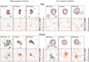 |
Fig. 5. Three representative spectral channels at velocities 180, 0, −180 km s−1, for the disk Petunia (upper panels) and the merger Adenia (bottom panels) at 60 deg. The left and right subfigures show the high S/N ALMA mock data at high and low-angular resolution. For each subfigure: the upper row shows the data (black contours) and the 3DBAROLO model (red contours). The contour levels are at 2.5, 5, 10 times the rms noise per channel. The gray ellipses in the first panels denote the synthetized beam of the observations. The bottom row shows the residuals normalized to the rms noise. |
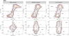 |
Fig. 6. Position-velocity diagrams along the kinematic major (upper panels) and minor axis (bottom panels) for the disk Petunia at 60 deg. The horizontal axis shows the offset from the galaxy center, and the vertical axis represents the line-of-sight velocity centred at the systemic velocity of the galaxy. From left to right, the high S/N ALMA mock data at high-, medium- and low-angular resolutions are shown. The black and red contours show the data and the 3DBAROLO model, respectively. The level contours are at −2.5, 2.5, 5 and 10 times the rms noise. The orange circles show the best-fit rotation velocities (not corrected for inclination) derived using 3DBAROLO. |
To estimate the capability of 3DBAROLO to recover reliable kinematic parameters for both high- and low-angular resolution observations, we computed the relative errors for the rotation velocity:
 (2)
(2)
where Vbest is the radial average at of the best-fit values derived with 3DBAROLO from the flat part of the rotation curve (R greater than the half-light radius). Vsim is computed after extracting the rotation curve from a slit on the moment-1 map of the edge-on view of the simulated galaxy (noise-free and not convolved).
Similarly, the relative errors for the velocity dispersions are computed as
 (3)
(3)
where σbest is the radial average of the best-fit values derived with 3DBAROLO and σsim is the average velocity dispersion from the moment-2 map of the face-on view of the simulated galaxy (noise-free and not convolved; see Col. 2 in Fig. 2 of Kohandel et al. 2020 as an example). The selection of face-on view for determining the intrinsic value of velocity dispersion from the simulation is to minimize the contribution of bulk motions such as rotation to the observed σ. In Fig. 8, the filled markers show the values of ϵV (upper panel) and ϵσ (bottom panel) for all mock data created from the three disks and the disturbed disk Freesia as a function of resolution. The relative errors are within 25% (gray area) in all cases, similar to the values reported in Di Teodoro & Fraternali (2015) for the tests on low-resolution observations of low-z galaxies. In the same figure, the empty markers show the relative errors when σbest and Vbest are obtained by using a 2D technique for correcting a posteriori for beam-smearing, the velocity gradient method (see Appendix B for details). With this method, the velocity gradients across the beam in the moment-1 maps are subtracted linearly from the corresponding moment-2 maps, while no correction for beam-smearing is applied to the rotation velocity profiles. The latter are extracted along the kinematic axes of the moment-1 maps in apertures equivalent to the beam and corrected for the inclination of the galaxies. The relative errors for the rotation velocities ϵV are within 25% (gray area) in most cases. However at low-angular resolutions, Vbest are systematically biased to values lower than the intrinsic ones and the values of ϵV are of −50% to −90% in some cases. On the contrary, the average velocity dispersions are strongly biased to values larger than the intrinsic ones (σsim), that is, the relative errors ϵσ reach values up to ∼200% at low-angular resolutions.
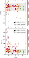 |
Fig. 8. Relative errors of the recovered rotation velocities (upper panel) and velocity dispersions (bottom panel), computed using Eqs. (2) and (3) for the disturbed disks Freesia (diamonds) and the three disks (squares) of our sample as a function of resolution (number of independent resolution elements along the semi-major axis). Markers with the same color show the mock data for the same galaxy as indicated by the color-bar. The filled and empty markers show the errors for the rotation velocities and velocity dispersions obtained with 3DBAROLO (forward-modeling) and with the velocity-gradient beam-smearing correction. The gray areas mark the 25 percentage. |
Mergers. At high-angular resolution (NIRE ≳ 4), the chi-square values are a factor of ≳10 higher than those for disks at similar resolutions and S/N. The presence of two interacting systems, strong asymmetries, tidal features is evident in the data cubes, the PV diagrams, and the moment maps. Therefore, the disk model created by 3DBAROLO is not able to reproduce the data, thus large residuals up to 40 rms appear in some spectral channels (see bottom left panels in Fig. 5 as a representative example for the merger Adenia). As the resolution decreases, there are fewer residuals in all spectral channels (see bottom right panels in Fig. 5), and the PV diagrams appear more regular and symmetric (right panels in Fig. 7, see also Figs. D.1 and D.2). However, the residuals of both the spectral channels and the PV diagrams are typically higher in the merger sample than the disk sample by a factor of ≈2. This is further discussed and quantified in Sect. 7.1.
6. Kinematic classification from the literature
In this section, we summarize the most common methods that have been used in the literature to characterize the dynamical state of high-z galaxies using emission-line observations. We then discuss the application of these methods to the mock data of SERRA galaxies and their ability to identify the fraction of disks in our sample correctly. The classification schemes described in Sects. 6.1 and 6.2 are quantitative as their criteria are based on comparing kinematic measurements and physically or empirically defined thresholds. Such methods can be applied to the 84 mock data a) – d) described in Sect. 4 and analyzed in Sect. 5, having quality good enough for constraining a kinematic model. On the contrary, the method described in Sect. 6.3 has been developed for classifying low-quality data: it is qualitative and mainly based on visual inspections of the kinematic maps. Accordingly, we adopt this method only on the 18 barely resolved mock data, i.e., whose low angular resolution and S/N did not allow for recovering any kinematic properties (point e) in Sect. 4).
In Table 3, we provide a summary of the data sets used for the analysis, the outcome, and recommendations on the data quality required to apply a given classification method.
Summary of the application of the classification techniques on our sample of mock data.
6.1. Smooth velocity fields and V/σ ratios
The most widely used method to classify high-z star-forming galaxies is based on the visual inspection of the velocity maps and the computation of the V/σ ratio (e.g., Wisnioski et al. 2015, 2019; Smit et al. 2018). Galaxies are classified as rotating disks if at least the following two criteria are satisfied: 1. moment-1 map with a smooth velocity gradient; 2. enough rotation support, i.e., V/σ > 1.8 (e.g., Wisnioski et al. 2015, 2019). Galaxies with a smooth velocity map but with V/σ < 1.8 (e.g., Förster Schreiber et al. 2009; Law et al. 2009; Kassin et al. 2012; Jones et al. 2021) are classified as dispersion-dominated systems, while galaxies with irregularities and no clear disk-like pattern in their velocity fields are mergers. These kinematic criteria have been used for both IFU and interferometric data and in a wide range of redshifts, from z ∼ 0.6 up to z ∼ 7–8 (e.g., Förster Schreiber et al. 2009; Wisnioski et al. 2015; Harrison et al. 2017; Stott et al. 2016; Smit et al. 2018; Bakx et al. 2020).
These two criteria set the minimal requirements to identify disk-like systems. Other three, increasingly strict, criteria can help to constrain the fraction of disks and mergers when high data quality and/or rest-frame spatially resolved optical maps are available (Wisnioski et al. 2015, 2019; Förster Schreiber et al. 2018). These additional criteria are the following: 3. the position of the steepest velocity gradient coincides with the peak of the velocity dispersion map; 4. the difference between the photometric and kinematic position angle is less than 30 deg; 5. the position of the steepest velocity gradient is coincident with the centroid of the stellar continuum center (Flores et al. 2006; Contini et al. 2016). SERRA galaxies with a smooth velocity field have a peak in the velocity dispersion map coincident with the position of steepest velocity gradient, automatically fulfilled criterion 3. However, the application of criteria 4. and 5. on SERRA galaxies, is not discussed in this work as our goal is to investigate whether we can constrain the dynamical stage of galaxies when only emission line observations are available (Jones et al. 2021).
To test whether this kinematic classification can distinguish the dynamical variety of our sample, we visually inspected the velocity fields of the mock data and computed the V/σ ratios from the maximum value of the rotation velocity profiles and the median value of the velocity dispersion profiles. In Fig. 9, we show the values of V/σ obtained both with 3DBAROLO (filled markers) and by using the velocity gradient beam-smearing correction (empty markers) for the disks and mergers of our sample. The key results of this analysis are the following.
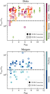 |
Fig. 9. V/σ ratio as a function of resolution (number of independent resolution elements along the semi-major axis) for the disks and the disturbed disk (upper panel) and the mergers (bottom panel). Markers with the same color show the mock data for the same SERRA galaxy as indicated by the color-bar. The black dashed line shows the threshold at 1.8. The filled markers show the V/σ ratios obtained with 3DBAROLO that is a 3D forward-modeling approach is applied to correct for the beam-smearing effect. The empty markers show the V/σ obtained when a velocity-gradient method is employed to correct for the beam-smearing effect. |
-
The velocity fields of the mock disks and the disturbed disk Freesia have a smooth gradient and V/σ ratios larger than 1.8 when the 3DBAROLO best-fit parameters are used. In other words, all disks passed the disk criteria when V and σ are derived using the forward-modeling technique. However, the V/σ ratios derived using the a posteriori beam-smearing correction are systematically lower than those derived using 3DBAROLO. In this case, at low resolution (NIRE≲ 2), the fraction of disks with V/σ > 1.8 is 50%, since the inferred velocity dispersions are significantly boosted and the inferred rotation velocities are underestimated due to the beam-smearing effect. Therefore, this combination leads to the misclassification of genuine disk galaxies as dispersion-dominated.
-
The velocity fields of the merger systems appear smooth or irregular depending on the data quality (angular resolution and S/N ratio), merger stage, and inclination. For example, at high-angular resolution (NIRE ≳ 3) the velocity field of the interacting system Adenia at i ∼ 60 deg appears irregular or disk-like depending on the S/N ratios (Cols. 2–4 and 6–7 in Fig. 4). However, the high S/N does not prevent the misclassification of Adenia as a disk at low-angular resolution at all inclinations (e.g., Col. 5 in Fig. 4). The mock data for the merging system Fuchsia have, instead, a smooth gradient in the velocity field only at low-angular resolution (NIRE ≲ 2) at i ∼ 60 deg and i ∼ 80 deg. At i ∼ 30 deg, Fuchsia has an irregular velocity field at all S/N and angular resolutions. As a reference, the V/σ ratios5 of the mergers cover a large range, from 0.4 to 5 and, contrary to the disks, there is no systematic difference between the values derived with the 2D and 3D beam-smearing correction methods.
-
In Fig. 10 (left panel), we show the fraction of mergers passing the two criteria used for identifying disks, i.e., smooth velocity fields (cyan bars) and V/σ > 1.8 (blue bars). The red bars show the fraction of mergers that satisfy both the criteria and are hence misclassified as disks. At the typical angular resolutions of high-z observations (NIRE ≲ 2), the fraction of mergers misclassified as disks is 50%. The main reason for this behavior is that the moment maps are smoother and more regular as the resolution decreases. Our results are in agreement with the findings of Simons et al. (2019), who show that at the typical angular resolutions of z ∼ 2 IFU observations, merger galaxies pass the disk criteria with a probability from 10 to 100% depending on the line of sight.
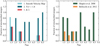
Fig. 10. Fraction of mergers classified as disks based on the criteria described in Sects. 6.1 (left, red bars) and 6.2 (right) as a function of resolution. In the left panel, the light blue and dark green bars show the fraction of galaxies with smooth velocity maps and V/σ ≳ 1.8. The latter are obtained using the velocity-gradient method for correcting for beam smearing. The non-zero fraction at NIRE ∼ 7.5 is due to the low S/N mock data. In the right panel, we show the fractions obtained using the Shapiro et al. (2008) and Bellocchi et al. (2012) methods as green and orange bars, respectively. Using the classification method described in Sect. 6.1, the only non-zero fraction of misclassified disks is obtained for NIRE ≲ 2 when the velocity-gradient method is used for correcting for beam smearing. In this case, 50% of disks are classified as dispersion-dominated systems. Using the kinemetry-based method all disks are correctly classified.
6.2. Kinemetry-based methods
Developed by Krajnović et al. (2006), the kinemetry method divides the moment-1 and moment-2 maps into concentric elliptical tilted rings from which azimuthal kinematic profiles are extracted and expanded into a finite number of harmonic terms
 (4)
(4)
where  and ϕi = arctan(Ai/Bi). For an ideal rotating disk, the only non-zero terms in the moment-1 maps are A0, corresponding to the systemic velocity, and B1, corresponding to the circular velocity. In the moment-2 maps, the only non-zero term is expected to be A0, describing the variation of the velocity dispersion as a function of radius. Therefore, asymmetries in the velocity and velocity dispersion maps are quantified by the presence of non-zero higher-order coefficients.
Shapiro et al. (2008) proposed to use the average values ki, avg, v(R) and ki, avg, σ(R) of the higher-order coefficients6, to define the velocity and velocity dispersion asymmetry parameters,
 (5a)
(5a)
 (5b)
(5b)
In Eqs. (5), the sum is over the number of rings N into which the velocity and velocity dispersion maps are divided. By using a series of template galaxies, cosmological simulations and actual observations of local disks and mergers, Shapiro et al. (2008) defined an empirical threshold for the global asymmetric parameters,  : galaxies with Kasym > 0.5 are classified as mergers, while galaxies with Kasym < 0.5 are disks. Using these criteria, the success rate in the correct classification of disks and mergers was estimated to be 89% and 80%, respectively (Shapiro et al. 2008).
Bellocchi et al. (2012) propose a modified computation of the asymmetry parameters, vasym, w and σasym, w, by giving more weight to asymmetric motions in the outer regions of galaxies. The global weighted asymmetric parameters,  should identify post-coalescence mergers, characterized by small asymmetries in the inner regions and outskirts with strong irregularities. Bellocchi et al. (2012) and Bellocchi et al. (2016) adopted IFU observations from a sample of local ultra-luminous galaxies to define an empirical division of mergers and disks at Kasym, w = 0.19. However, they noticed that this value changes with the resolution: by redshifting their sample to z = 3, the value of Kasym, w distinguishing the two kinematic classes is 0.16.
We can use our data sample to quantify the success rates in the kinematic classification for both Shapiro et al. (2008) and Bellocchi et al. (2012) methods. To define the rings used for the kinemetry decomposition, we assumed the best-fit center, inclination, and position angles found by 3DBAROLO. The resulting Ai and Bi coefficients are then used to compute the asymmetry parameters and the values of Kasym and Kasym, w. In Fig. 11, we show the global asymmetric parameters obtained using the definition from Shapiro et al. (2008) and Bellocchi et al. (2012) as a function of resolutions for our mock data. The key findings from the application of the kinemetry analysis are the following:
-
100% of the disks are correctly classified by using both the criteria defined in Shapiro et al. (2008) and Bellocchi et al. (2016). However, the values of Kasym, w are consistent with the threshold of 0.16 for most galaxies at low angular resolution. On the contrary, the values of Kasym are on average a factor of 5 lower than the threshold of 0.5.
-
The same results are valid for the disturbed disk Freesia, except for the Ideal Mock at i = 30 deg, which features a value of Kasym, w = 0.3. For this line of sight and with the high sensitivity and angular resolution of the Ideal Mock, the Bellocchi et al. (2016) method is able to identify the asymmetric motions in the faint outer regions of this galaxy.
-
In Fig. 10 (right panel), we show the fraction of mergers misclassified as disks according to the Shapiro et al. (2008) and Bellocchi et al. (2016) criteria. The latter is optimal for identifying the mergers of our sample at NIRE ≳ 4. On the contrary, the Shapiro et al. (2008) method misclassifies mergers up to 100% even for high-resolution observations. Bellocchi et al. (2016) already noticed that the limit of Kasym = 0.5 proposed by Shapiro et al. (2008) lead to misclassify more than 50% of the post-coalescence mergers, while a limit of Kasym = 0.14 is optimal for increasing the success rate of the merger identification (see also discussion in Shapiro et al. (2008) and Bellocchi et al. (2012) about the Kasym limit for further details). If we use this limit of Kasym = 0.14, we obtain a fraction of misclassified mergers similar to that obtained by using the Bellocchi et al. (2016) method. In other words, with the appropriate tuning of the threshold, the global asymmetric parameters Kasym and Kasym, w perform equally well in distinguishing between disks and mergers when high-angular resolution data are employed.
-
At low angular resolution (NIRE ≲ 3.5), the asymmetries in the velocity and velocity dispersion maps are washed out. The fraction of our mergers misclassified as disks range from 30 to 80%, based on the Bellocchi et al. (2016) and Shapiro et al. (2008) methods, respectively. The latter is in agreement with the results of Gonçalves et al. (2010), which reported a similar fraction of misclassified galaxies for a sample of z ∼ 2.2 simulated galaxies. Shapiro et al. (2008) and Wisnioski et al. (2015) had already noticed that the most critical requirement in applying the kinemetry analysis is that the galaxy should be “well resolved”, with however no clear consensus on its definition. Shapiro et al. (2008) defined a well-resolved galaxy to be covered by at least 3 resolution elements, while Wisnioski et al. (2015) report a value of 10 resolution elements. Our tests indicate that at least 8 independent resolution elements along the maximum extension of the galaxy (i.e., major-axis) are needed to identify the presence of interacting galaxies correctly.
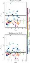 |
Fig. 11. Global asymmetric parameters as a function of resolution for the disks (squares), mergers (circles), and the disturbed disk Freesia (diamonds). The global asymmetric parameters are computed according to the definitions of Shapiro et al. (2008) (upper) and Bellocchi et al. (2012) (bottom). The solid black and dashed gray lines in the upper panel show the limit of 0.5 and 0.14, indicated by Shapiro et al. (2008) and Bellocchi et al. (2016) as the thresholds for distinguishing between disks and mergers, respectively. In the bottom panel, the solid and dashed black lines show the limits of 0.19 and 0.16, indicated by Bellocchi et al. (2016) as the discriminators between disks and mergers at low and high-z, respectively. |
6.3. Qualitative method
At z ≳ 4, a systematic kinematic classification of star-forming galaxies was performed using the ALPINE sample (Le Fèvre et al. 2020; Romano et al. 2021; Jones et al. 2021). However, similar to most observations of galaxies at z ≳ 4 (e.g., Smit et al. 2018; Bakx et al. 2020), most of the ALPINE sample is barely resolved since the survey has been designed mainly for line detection. As shown in Jones et al. (2021), only for part of the sample (14/75 galaxies), the S/N is high enough to adopt a quantitative kinematic classification (the one described in Sect. 6.1).
For the entire sample, Romano et al. (2021) and Le Fèvre et al. (2020) provide a qualitative classification by dividing galaxies into: mergers, disks, dispersion-dominated, and uncertain. In the classification scheme of Romano et al. (2021) and Le Fèvre et al. (2020), mergers are galaxies showing irregular morphologies in the moment-0 maps, PV diagrams or optical images (when available, see discussion in Sect. 6.1); disturbed moment-1 maps; global line profile fitted by multiple components. The disk class includes galaxies characterized by detection of the emission in contiguous channel maps; a gradient in the moment-1 maps; PV diagrams along the major axis with tilted emission; straight emission in the PV diagrams along the minor axis; possible double-horn profile; a single component in the optical images. Galaxies with no positional shifts of emission across channel maps; straight emission in the PV diagrams; a Gaussian line profile are assigned to the dispersion-dominated class.
Applying the kinematic criteria described in Romano et al. (2021) and Le Fèvre et al. (2020) requires a visual inspection of the moment maps, PV diagrams along the major and minor axis, and the integrated spectrum. Starting from the ALMA barely resolved mock cubes, we created the kinematic maps and profiles using the method described in Romano et al. (2021) and summarized here:
-
The moment-1 and 2 maps are obtained after masking all pixels below 3 rms in the moment-0 map.
-
The moment-0 map is fitted using a two-dimensional Gaussian profile. The best-fit center is then used to extract the PV diagrams along the major and minor axis. The latter is oriented along the direction of the strongest velocity gradient in the velocity map.
-
The [C II] integrated spectrum is obtained after extracting the flux in the aperture defined by the 3 rms-mask on the moment 0 map. One or multiple Gaussian components are used to fit the spectra.
In Fig. 12, we show the [C II] integrated spectrum (gray line) and its best-fit model (solid green line), the moment maps, and the PV diagrams for one representative disk galaxy, the system Opuntia at three inclinations. Similar kinematic maps and profiles are shown in Fig. 13 for the disturbed disk Freesia and the mergers Adenia and Fuchsia at i = 60 deg.
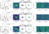 |
Fig. 12. Kinematic maps and profile for the barely resolved ALMA mock data for the disk Opuntia at 30 (upper panels), 60 (medium panels) and 80 deg (bottom panels). Column 1: [C II] integrated spectrum (gray histogram) and best-fit model (solid green line), resulting from the sum of two components (red dashed and purple dotted lines). Column 2: moment-0 map with black contours showing the 3, 6 and 9 rms levels. Columns 3 and 4: moment-1 and moment-2 maps obtained following the methodology in Romano et al. (2021) (see Sect. 6.3 for details). The dashed lines in the moment-1 map show the directions of the major and minor axis along which the PV-diagrams are extracted. Columns 5 and 6: PV diagrams along the major (left) and minor (right) axis with contours at −2 rms (dashed gray lines) and 2, 4, 8 rms (solid black lines). |
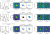 |
Fig. 13. Same as in Fig. 12, but for the disturbed disk Freesia and the merging systems Adenia, Fuchsia at i = 60 deg. |
The key findings resulting from applying the qualitative method are the following.
-
Eight out of nine disks are classified as mergers, with the only exception of Opuntia at i ∼ 80 deg that is classified as a dispersion-dominated galaxy. At i ∼ 30 and 60 deg, Opuntia is classified as a merger as two Gaussian components describe the integrated spectra, the velocity and velocity dispersion maps are disturbed, the PV diagrams along the major axis show two components at 3 rms separated in velocity by at least 200 km s−1 and with a spatial offset. At i ∼ 80 deg, the integrated spectrum is, instead, well described by a single Gaussian line profile, and the PV diagrams are straight both along the major and minor axis. The misclassification of disk galaxies due to the low-quality data is also discussed in Förster Schreiber et al. (2018), where they show the changes in the velocity field features as a function of S/N.
-
The disturbed disk, Freesia, is classified as a disk at all inclinations.
-
Adenia is correctly classified as a merger at all inclinations due to the multiple components in the integrated spectra and the PV diagrams.
-
The merging system, Fuchsia, is classified as a dispersion-dominated galaxy at all inclinations due to the presence of a single component in the integrated spectra and straight PV diagrams.
To summarize, 100% of the disks in our sample are misclassified as mergers or dispersion-dominated galaxies and only 50% of the mergers are correctly identified. Even though an accurate statistical analysis is not feasible due to the low number of our mock data, the result advises against the adoption of the qualitative kinematic classification for low-quality data. This could be improved by considering the information from optical/UV maps, but it is out of the scope of the present work (see Sect. 6.1).
7. PVsplit: A new 3D kinematic classification
When a forward-modeling technique is adopted, robust kinematic parameters can be recovered even at low-angular resolutions and S/N ≳ 5 for disk galaxies (Sect. 5.2). However, with this data quality, the different techniques adopted so far failed in identifying the merging systems (Sect. 6) since the methods mainly use the information contained in the moment-1 and 2 maps. For example, one of the best classification schemes tested with our sample, the Bellocchi et al. (2012) method, requires data at NIRE ≳ 4 to guarantee a robust characterization of the dynamical state of a galaxy. With the sensitivities of the current instruments (e.g., ALMA), such high angular-resolution data with a minimum S/N of ∼5 require an integration time on the source of at least 30 hours for a typical Lyman break galaxy at z ∼ 6. Due to the typical observing time constraints for current programs, high-angular resolution observations can be obtained in the near future only by targeting a handful of Lyman break galaxies at a time.
In this section, we present a proof-of-concept analysis aiming to show that a robust kinematic classification of a galaxy is still feasible with medium- and low-angular resolution data. The technique is called “PVsplit”, the main novelty is that it is based on the analysis of PV diagrams rather than using moment-1 and 2 maps.
7.1. PV parameters
Based on the symmetry and morphology of the PV diagrams along the major and minor axes, we can define five new empirical parameters. A schematic representation of their main features is shown in Fig. 14 and a formal definition is given in the following:
-
quantifies the asymmetry of the major axis PV diagram with respect to the horizontal axis defining the systemic velocity. The latter divides the PV diagrams into two regions: A1 and A2 (see Fig. 14). The parameter is defined as
![Mathematical equation: $$ \begin{aligned} P_{\mathrm{major} }=\log \left[ \frac{\sum _i (F_{A1,i}-F_{A2^*, i})^2}{\sum _{i} (F_{A1, i}+F_{A2^*, i})^2} \right] \end{aligned} $$](/articles/aa/full_html/2022/11/aa43582-22/aa43582-22-eq13.gif) (6)
(6)where FA1, i and FA2*, i are the fluxes in the pixels i of the region A1 and A2*, respectively. The latter is the reflection of the region A2 with respect to the center. For an ideal rotating disk, A2* = A1, thus Pmajor = 0.
-
evaluates the asymmetries of the minor-axis PV diagram with respect to the systemic velocity (e.g., horizontal dashed line in Fig. 6, bottom panels; see Sect. 5.2 for a discussion about the minor-axis PV diagram of a rotating disk).
-
is similar to Pminor, 1, but for quantifying the asymmetries of the minor-axis PV diagram with respect to the center (e.g., vertical dashed line in Fig. 6, bottom panels).
-
is specifically suited for medium and low-resolution observations. The emission peak in the PV diagrams has distinct morphologies in the disks and mergers both at high and low angular resolutions. The major-axis PV diagrams of the disks have a narrow emission peak along the velocity axis at values close to the line-of-sight velocities at the outermost radii of the galaxy, Vlos, out. Instead, for mergers, the peaks, corresponding to the two interacting systems, are i) spread over a large range of line-of-sight velocities, or ii) have a narrow distribution closer to the systemic velocity than to Vlos, out. For quantifying these different distributions of the emission peaks along the velocity axis of the PV diagrams, we first selected the 20% brightest pixels in the regions A1 and A2 separately (see discussion in Appendix D for further details on this assumption). These pixels are used to compute PV as
![Mathematical equation: $$ \begin{aligned} P_{{V}} =\log \left| {\mathrm{Mean}_{A1,A2}} \left[ \frac{V_{\mathrm{ctr}}}{V_{\mathrm{los, out}}} \exp {\left(-\frac{\Delta V}{V_{\mathrm{ctr}}}\right)} \right] -1 \right|, \end{aligned} $$](/articles/aa/full_html/2022/11/aa43582-22/aa43582-22-eq14.gif) (7)
(7)where Vctr is the flux-weighted average line-of-sight velocity, ΔV is the difference between the 97.7% and 2.3% of the peak distributions along the velocity axis. The mean in Eq. (7) is over the two values of PV obtained for the regions A1 and A2. The maximum value is considered when multiple, distinct emission peaks are identified in A1 and A2. The exponential term is close to 1 in the case of a narrow emission peak distribution, typical of a disk, and it is ≫1 for a peak emission spread over a large range of velocities, typical of a merger.
-
is similar to PV but for the distribution of the emission peak along the radial axis. To describe this empirical parameter, we define the two quadrants l and r over which the vertical line defining the center of the major-axis PV diagrams splits the regions A1 and A2 into two parts. The emission peak covers either quadrant l or r for the disks. Instead, for the mergers, the emission peak covers a region that is spread over both the l and r quadrants, or it is closer to the center than to the outermost radius used for the extraction of the kinematic parameters, Rext. To define PR, we used the following equation:
 (8)
(8)
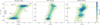 |
Fig. 14. Schematic representation of the morphological and symmetrical features in the major axis PV diagrams considered for the computation of the P parameters defined in Sect. 7.1. Left panel: PV diagram for a representative thin rotating disk model along the major axis. The dotted gray horizontal line shows the position of the systemic velocity that divides the major-axis PV diagram into regions A1 and A2, while the dotted gray vertical lines indicate the center dividing A1 and A2 into two regions, l and r. The ith representative pixels used for the computation of Pmajor are shown in the regions A1 and A2, respectively. The blue dotted contours enclose the 20% brightest pixels, and the yellow crosses are their flux-weighted centroids. The black plus indicates the outermost radius used for the extraction of the kinematic parameters, and the solid orange lines are Vlos, out, the average values of the galaxy line-of-sight velocities. The double arrow indicates ΔV, the extension along the velocity axis for one of the peak distributions. The major-axis PV diagrams from the high S/N, low-resolution mock data of the disk Lantana and merger Adenia are shown in the central and right panels. |
where Rctr is the flux-weighted average radial position of 20% brightest pixels in the regions A1 and A2.
To measure the PV parameters for our mock data, we used the PV diagrams extracted along the best-fit major and minor axes found with 3DBAROLO. Since, as discussed in Sect. 5, the kinematic fitting is not feasible for the barely resolved mock data (point e) in Sect. 4), they are excluded from the analysis and discussion in this Section.
7.2. Construction of the classifier
The PV parameters defined in Sect. 7.1 have different trends as a function of the resolution: this complex situation can be appreciated in Fig. 15.
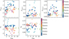 |
Fig. 15. PV parameters described in Sect. 7.1 as a function of the independent resolution elements along the semi-major axis (Appendix A for details). |
Visual inspections indicate that Pminor, 1 and Pminor, 2 – the asymmetric parameters along the minor axis – have overlapping values for disks and mergers, regardless of the resolution (e.g., Figs. D.1 and D.2). Furthermore, at the typical surface brightness distribution and kinematic properties of disks (e.g., exponential profiles, flat rotation curves), the minor axis PV diagrams have S/N smaller than the major-axis PV diagrams as less number of channel maps typically contribute to their emission. This means that even for rotating disks, asymmetries in the minor-axis PV diagrams can appear because some regions are below the noise levels. Instead, the disk and merger populations seems to be located in different regions for the parameters Pmajor, PV, and PR. In particular, Pmajor seems able to clearly distinguish between disks and mergers when NIRE ≳ 3; however, for low resolution (NIRE ≲ 3), both disks and mergers have values of Pmajor ≲ 0.25, that is, the major-axis PV diagrams of the mergers are as symmetric as PV diagrams for disks.
The insight given by this visual inspection can be formalized by constructing a machine learning (ML) classifier. We build a classifier based on a decision tree using the SCIKIT-LEARN implementation (Pedregosa et al. 2012). In general, a decision tree is a data-driven (supervised) ML algorithm: given a set of parameters (features in the ML language), and a discrete number of classes (labels in ML), the algorithm splits the parameter space into sub-volumes with maximal information content; the final goal of the algorithm is to predict the class with arbitrary parameters, i.e., that have not been used in the construction of the tree. Our classes are merger and disk, and we select the 5 PV parameters described in Sect. 7.1 and use the 84 galaxies as our data set. By dividing the sample randomly, 70% of the data is used as training in the construction of the algorithm, 30% as a testing set.
The resulting decision tree has a R2 score of 84%, i.e., it is reasonably reliable in distinguishing between disk and mergers, given the small data set we are adopting here. We then checked the feature importance of our parameters in distinguishing if a galaxy is a disk or a merger. In Fig. 16 we plot the importance of each PV parameter used in the ML. Both Pminor, 1 and Pminor, 2 appear to have negligible importance, while Pmajor, PR and PV are dominant in determining the kinematic class of the galaxy. These results confirm our visual intuition. However, we have to extend the size of the data set to build a more reliable classifier (e.g., R2 ≳ 95%) and eventually explore the importance of additional parameters in the PV space; this is left for future work.
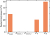 |
Fig. 16. Importance of the different PV parameters for the disk/merger classification. The fractional importance is computed for the different parameters (definitions in Sect. 7.1) by constructing a decision tree classifier to distinguish between disks and mergers. The decision tree uses our sample of 84 galaxies with different resolutions and S/N, using 70% (30%) of the data for training (testing), resulting in a R2 score of 84%. |
In Fig. 17, we show the position of the 84 mock SERRA galaxies in the 3D parameter space, defined by the three parameters with higher importance, i.e. Pmajor, PV, PR. The merger (Adenia, Fuchsia) and disk systems (Opuntia, Lantana, Petunia) are clearly clustered in two different regions. The disturbed disk Freesia (diamonds) data is spread over the disk and merger regions: at low resolution, the galaxy behaves like a disk, while at high resolution, the galaxy is classified as a merger, depending on the inclination.
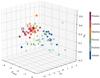 |
Fig. 17. Position of the 84 mock data (squares: disks, circles: mergers; diamonds: disturbed disk Freesia) in the PVsplit parameter space. The empty black square and circle show the position of a spiral and a merger galaxy at z = 0, respectively. A movie with a 3D visualization of this figure is available online. |
Although tested on EoR galaxies, PVsplit should be valid at any redshifts as it relies on the morphology of the major-axis PV diagrams. These are expected to have specific features in case any gas rotation is present (e.g., S-shape profile, equivalent to the velocity gradient in the moment-1 maps). As a validation, we computed the PV parameters from real observations of a prototypical disk and a merger at z = 0 (see Appendix C for details):
-
The spiral galaxy, NGC 2403, for which we used HI observations at low-angular resolution (empty black square, de Blok et al. 2014).
-
The Antennae galaxy, a prototypical example of a merger system in the local Universe, as observed at low-angular resolution. ALMA Science Verification observations of the CO(3-2) emission line are employed for creating these data7.
The low-z spiral and the Antennae galaxy are in the disk and merger regions defined by the SERRA disks and merger distributions, respectively (empty markers in Fig. 17). This analysis shows that by using PVsplit on data with S/N ≳ 10 and with at least 3 independent resolution elements along the major axis, one can distinguish whether a galaxy is a disk or a merger in a way that is independent of the redshift and tracers employed to measure the kinematics. A summary of the data sets used for the analysis of PVsplit, the main results, and recommendations on the required data quality is shown in Table 3.
7.3. Advantages of PVsplit
As discussed in Sect. 6, the common feature of the classification methods mostly used until now is the analysis of moment maps, which are projections of the data cubes to 2D space obtained after masking low S/N pixels in each spectral channel. In these 2D maps, the possibility to constrain the presence of non-circular motions driven by interactions strongly depends on the quality of the data. At medium and low-angular resolution, most asymmetries in the moment maps are smoothed out so that identifying a merging system becomes challenging.
The main novelty of PVsplit with respect to the standard classification methods is that it leverages the constraints on the dynamical stages of galaxies contained in the cubes, the native space of the data, through the analysis of the PV diagrams. The latter can be considered a more accurate representation of the data cubes since they require only to define the position angle along which they are extracted. In addition to the symmetrical properties of the PV diagrams along the major axis, PVsplit relies on the morphological features of the emission peaks. The latter is especially crucial at the low-angular resolution, showing that the non-circular motions driven by interactions are still imprinted in the data.
Despite the mock data from six galaxies at three different inclinations, we expect that the main conclusions of the PVsplit analysis would be valid also on a larger sample of galaxies as the PVsplit parameters are based on the morphological characterization of the major-axis PV diagrams of rotating disks. The latter have an S-shape profile, the equivalent of the velocity gradient in the velocity field, regardless of the redshift, surface brightness distributions and velocity dispersion profiles. We note, in fact, that one of the main difference between rotating disks at different redshifts is the level of velocity dispersion, that is, galaxies at high-z receive considerable support from random motions in comparison to the local Universe (Förster Schreiber & Wuyts 2020). However, high velocity dispersion values make the distribution of the galaxies in the PV diagrams thicker but they do not change the S-shape profiles in the case of rotating disk galaxies.
8. Summary
Characterizing the dynamical state of galaxies is one of the critical steps to constrain their mass assembly history. This is particularly crucial in the early Universe, where the build-up activity was considerably accelerated with respect to the present-day rate. We are now entering a new era for this field since thousands of galaxies up to z ∼ 7 will be discovered with the current and future facilities (e.g., JWST, WFIRST, Euclid, Mason et al. 2015; Cuby et al. 2019; Vogelsberger et al. 2020). These datasets will be a pool for finding the ideal targets for spatially resolved follow-up observations. Defining an observational strategy to constrain the growth of these first galaxies is critical to fully taking advantage of this opportunity.
In this paper, we analyzed the performance of three methods commonly used to constrain the dynamical properties of intermediate- and high-z galaxies depending on angular resolution and S/N of the data. We have used six z ∼ 6–7 Lyman break galaxies at three inclination angles from the SERRA zoom-in cosmological simulation suite (Pallottini et al. 2022). The selected SERRA galaxies cover a range of dynamical states: three are isolated disks, one is a disturbed disk, and two are major mergers. We created mock observations of the [C II] emission with various data quality (Kohandel et al. 2020): from an ideal case with very high S/N and angular resolutions to ALMA mock data typical of line-detection surveys. The key findings are:
-
The qualitative classification scheme proposed by Romano et al. (2021) for low-SN and barely resolved data (i.e., for a given galaxy, the area at S/N ≳ 3 extends for less than 50% of the beam area in each spectral channel) may significantly underestimate the fraction of disk galaxies. We discourage any kinematic analysis on such observations since the resulting dynamical stages can be strongly biased and difficult to control, even when large statistics are available.
-
The classification scheme (smooth velocity field and V/σ ratio) proposed by Wisnioski et al. (2015) and Wisnioski et al. (2019) underestimates the fraction of disks when the values of V and σ are obtained using a 2D beam-smearing correction. On the contrary, the disks are correctly identified when a 3D forward-modeling technique is employed. The success rate of this method in identifying merging systems strongly depends on the S/N, even when high angular resolutions are used.
-
The kinemetry-based classification methods (Shapiro et al. 2008; Bellocchi et al. 2012) underestimate the fraction of mergers at the typical angular resolution of high-z observations. However, the Bellocchi et al. (2012) method is optimal for high-S/N and high angular resolution data (i.e., S/N ≳ 5 and at least 4 independent resolution elements along the semi-major axis of the galaxy), that is, with data quality currently available only for a handful of targets with the current facilities (e.g., ALMA).
-
Our analysis shows that the classical classification methods are sub-optimal to correctly characterize the dynamical stage as they analyzed the moment maps. This paper shows how a change of perspective is sufficient to overcome the limitations of the standard kinematic classification methods. Instead of the moment maps, the PV diagrams contain a wealth of information that allows accurate characterization of the kinematic state of a galaxy even at low-angular resolution. To quantify this, we introduced here a new classification method, PVsplit, that relies on three empirical parameters describing the asymmetry and morphological features of the PV diagram along the galaxy’s major axis. PVsplit requires a minimum of ≈3 independent resolution elements along the major axis of a galaxy and S/N, computed as the median of the maximum S/N in each spectral channel, of at least 10 to correctly identify its dynamical stage as a disk or a merger. With ALMA, such data quality can be achieved with an integration time of 7 h for a z ∼ 6 main-sequence galaxy with SFR ≃ 30 M⊙ yr−1 and L[CII] ≃ 3 × 10⁸ L⊙. In addition, PVsplit is applicable to galaxies at all redshifts and with kinematics derived from gas emission lines.
In the second paper of this series, we will expand our results of PVsplit on a large sample of simulated and observed galaxies with the aim of statistically evaluating the performance of this new method using a more extensive range of dynamical states. In that work, we will also discuss the position of observed low- and high-z galaxies in the PVsplit parameter space.
Movie
Movie 1 associated with Fig. 17 (PVsplit_fig16) Access Supplementary Material
We call a galaxy face-on when we orientate the l.o.s. parallel to the eigenvector of the inertia tensor of the gas mass distribution with the largest eigenvalue.
The S/N is computed as the median of the maximum S/N in each spectral channel.
Note that for the mergers, the resulting kinematic parameters (e.g., rotation velocity and velocity dispersions) do not have a physical meaning and thus can not be used to infer physical parameters of the galaxies (e.g., virial mass, dark matter halo mass)
The PV diagrams are slices extracted from data cubes along a specific spatial direction (e.g., the kinematic major axis).
Recall that V and σ for merger do not have a physical meaning since they are derived under the assumption that the fitting galaxy is a rotating disk (Sect. 4).
The higher-order coefficients ki, 2, v - ki, 5, v are used for the computation of ki, avg, v = (ki, 2, v + ki, 3, v + ki, 4, v + ki, 5, v)/4. ki, avg, σ is, instead, obtained by averaging the ki, 1, σ - ki, 5, σ, ki, avg, σ = (ki, 1, σ + ki, 2, σ + ki, 3, σ + ki, 4, σ + ki, 5, σ)/5.
Acknowledgments
F.R. thanks F. Fraternali for providing the HI data for NGC2403 and D. Krajnović for providing the python version of KINEMETRY. FR is grateful to F. Fraternali and M. Romano for useful comments and discussions. FR acknowledges support from the European Union’s Horizon 2020 research and innovation program under the Marie Sklodowska-Curie grant agreement No. 847523 ‘INTERACTIONS’ and the Cosmic Dawn Center that is funded by the Danish National Research Foundation under grant No. 140. M.K., A.P., A.F., L.V. acknowledge support from the ERC Advanced Grant INTERSTELLAR H2020/740120 (PI: Ferrara). Any dissemination of results must indicate that it reflects only the author’s view and that the Commission is not responsible for any use that may be made of the information it contains. We acknowledge the CINECA award under the ISCRA initiative, for the availability of high performance computing resources and support from the Class B project SERRA HP10BPUZ8F (PI: Pallottini). We gratefully acknowledge computational resources of the Center for High Performance Computing (CHPC) at SNS. This paper makes use of the following ALMA data: ADS/JAO.ALMA2011.0.00003.SV. ALMA is a partnership of ESO (representing its member states), NSF (USA) and NINS (Japan), together with NRC (Canada), NSC and ASIAA (Taiwan), and KASI (Republic of Korea), in cooperation with the Republic of Chile. The Joint ALMA Observatory is operated by ESO, AUI/NRAO and NAOJ. We acknowledge usage of the Python programming language (Van Rossum & de Boer 1991; Van Rossum & Drake 2009), Astropy (Astropy Collaboration 2013), Cython (Behnel et al. 2011), Matplotlib (Hunter 2007), numba (Lam et al. 2015), NumPy (van der Walt et al. 2011), PYNBODY (Pontzen et al. 2013), SCIKIT-LEARN (Pedregosa et al. 2012), and SciPy (Virtanen et al. 2020).
References
- Agertz, O., Kravtsov, A. V., Leitner, S. N., & Gnedin, N. Y. 2013, ApJ, 770, 25 [NASA ADS] [CrossRef] [Google Scholar]
- Asplund, M., Grevesse, N., Sauval, A. J., & Scott, P. 2009, ARA&A, 47, 481 [NASA ADS] [CrossRef] [Google Scholar]
- Astropy Collaboration (Robitaille, T. P., et al.) 2013, A&A, 558, A33 [NASA ADS] [CrossRef] [EDP Sciences] [Google Scholar]
- Bakx, T. J. L. C., Tamura, Y., Hashimoto, T., et al. 2020, MNRAS, 493, 4294 [NASA ADS] [CrossRef] [Google Scholar]
- Barnes, J., & Hut, P. 1986, Nature, 324, 446 [NASA ADS] [CrossRef] [Google Scholar]
- Behnel, S., Bradshaw, R., Citro, C., et al. 2011, Comput. Sci. Eng., 13, 31 [Google Scholar]
- Behroozi, P. S., Wechsler, R. H., & Wu, H.-Y. 2013, ApJ, 762, 109 [NASA ADS] [CrossRef] [Google Scholar]
- Bellocchi, E., Arribas, S., & Colina, L. 2012, A&A, 542, A54 [NASA ADS] [CrossRef] [EDP Sciences] [Google Scholar]
- Bellocchi, E., Arribas, S., & Colina, L. 2016, A&A, 591, A85 [NASA ADS] [CrossRef] [EDP Sciences] [Google Scholar]
- Bertelli, G., Bressan, A., Chiosi, C., Fagotto, F., & Nasi, E. 1994, A&AS, 106, 275 [NASA ADS] [Google Scholar]
- Béthermin, M., Fudamoto, Y., Ginolfi, M., et al. 2020, A&A, 643, A2 [Google Scholar]
- Bosma, A. 1978, PhD Thesis, Groningen University, The Netherlands [Google Scholar]
- Bouché, N., Carfantan, H., Schroetter, I., Michel-Dansac, L., & Contini, T. 2015, AJ, 150, 92 [Google Scholar]
- Bournaud, F., Elmegreen, B. G., & Elmegreen, D. M. 2007, ApJ, 670, 237 [Google Scholar]
- Bouwens, R. J., Illingworth, G. D., van Dokkum, P. G., et al. 2021, AJ, 162, 255 [NASA ADS] [CrossRef] [Google Scholar]
- Bouwens, R. J., Smit, R., Schouws, S., et al. 2022, ApJ, 931, 160 [NASA ADS] [CrossRef] [Google Scholar]
- Bovino, S., Grassi, T., Capelo, P. R., Schleicher, D. R. G., & Banerjee, R. 2016, A&A, 590, A15 [NASA ADS] [CrossRef] [EDP Sciences] [Google Scholar]
- Brodie, J. P., Romanowsky, A. J., Strader, J., & Forbes, D. A. 2011, AJ, 142, 199 [NASA ADS] [CrossRef] [Google Scholar]
- Burkert, A., Förster Schreiber, N. M., Genzel, R., et al. 2016, ApJ, 826, 214 [Google Scholar]
- Carniani, S., Ferrara, A., Maiolino, R., et al. 2020, MNRAS, 499, 5136 [NASA ADS] [CrossRef] [Google Scholar]
- Ceverino, D., Dekel, A., Tweed, D., & Primack, J. 2015, MNRAS, 447, 3291 [NASA ADS] [CrossRef] [Google Scholar]
- Ceverino, D., Glover, S. C. O., & Klessen, R. S. 2017, MNRAS, 470, 2791 [NASA ADS] [CrossRef] [Google Scholar]
- Cimatti, A., Fraternali, F., & Nipoti, C. 2019, Introductionto Galaxy Formation and Evolution: From Primordial Gas toPresent-Day Galaxies (Cambridge University Press) [Google Scholar]
- Contini, T., Epinat, B., Bouché, N., et al. 2016, A&A, 591, A49 [NASA ADS] [CrossRef] [EDP Sciences] [Google Scholar]
- Cuby, J.-G., Oesch, P., Cooray, A., et al. 2019, BAAS, 51, 360 [NASA ADS] [Google Scholar]
- Danovich, M., Dekel, A., Hahn, O., Ceverino, D., & Primack, J. 2015, MNRAS, 449, 2087 [Google Scholar]
- de Blok, W. J. G., Keating, K. M., Pisano, D. J., et al. 2014, A&A, 569, A68 [NASA ADS] [CrossRef] [EDP Sciences] [Google Scholar]
- Decataldo, D., Pallottini, A., Ferrara, A., Vallini, L., & Gallerani, S. 2019, MNRAS, 487, 3377 [Google Scholar]
- Dekel, A., Sari, R., & Ceverino, D. 2009, ApJ, 703, 785 [Google Scholar]
- Dekel, A., Lapiner, S., Ginzburg, O., et al. 2020, MNRAS, 496, 5372 [NASA ADS] [CrossRef] [Google Scholar]
- Di Teodoro, E. M., & Fraternali, F. 2015, MNRAS, 451, 3021 [Google Scholar]
- Di Teodoro, E. M., & Peek, J. E. G. 2021, ApJ, 923, 220 [NASA ADS] [CrossRef] [Google Scholar]
- Dubois, Y., Pichon, C., Haehnelt, M., et al. 2012, MNRAS, 423, 3616 [NASA ADS] [CrossRef] [Google Scholar]
- Duncan, K., Conselice, C. J., Mundy, C., et al. 2019, ApJ, 876, 110 [NASA ADS] [CrossRef] [Google Scholar]
- Ejdetjärn, T., Agertz, O., Östlin, G., Renaud, F., & Romeo, A. B. 2022, MNRAS, 514, 480 [CrossRef] [Google Scholar]
- Epinat, B., Amram, P., Balkowski, C., & Marcelin, M. 2010, MNRAS, 401, 2113 [Google Scholar]
- Federrath, C., & Klessen, R. S. 2013, ApJ, 763, 51 [Google Scholar]
- Federrath, C., Salim, D. M., Medling, A. M., et al. 2017, MNRAS, 468, 3965 [NASA ADS] [CrossRef] [Google Scholar]
- Ferland, G. J., Chatzikos, M., Guzmán, F., et al. 2017, Rev. Mex. Astron. Astrofis., 53, 385 [NASA ADS] [Google Scholar]
- Flores, H., Hammer, F., Puech, M., Amram, P., & Balkowski, C. 2006, A&A, 455, 107 [NASA ADS] [CrossRef] [EDP Sciences] [Google Scholar]
- Förster Schreiber, N. M., Genzel, R., Bouché, N., et al. 2009, ApJ, 706, 1364 [Google Scholar]
- Förster Schreiber, N. M., Renzini, A., Mancini, C., et al. 2018, ApJS, 238, 21 [Google Scholar]
- Förster Schreiber, N. M., & Wuyts, S. 2020, ARA&A, 58, 661 [Google Scholar]
- Fraternali, F., Karim, A., Magnelli, B., et al. 2021, A&A, 647, A194 [NASA ADS] [CrossRef] [EDP Sciences] [Google Scholar]
- Fraternali, F., Oosterloo, T., Sancisi, R., & van Moorsel, G. 2001, ApJ, 562, L47 [CrossRef] [Google Scholar]
- Fraternali, F., van Moorsel, G., Sancisi, R., & Oosterloo, T. 2002, AJ, 123, 3124 [CrossRef] [Google Scholar]
- Fujimoto, S., Silverman, J. D., Bethermin, M., et al. 2020, ApJ, 900, 1 [Google Scholar]
- Fujimoto, S., Oguri, M., Brammer, G., et al. 2021, ApJ, 911, 99 [Google Scholar]
- Glazebrook, K. 2013, PASA, 30, e056 [NASA ADS] [CrossRef] [Google Scholar]
- Gonçalves, T. S., Basu-Zych, A., Overzier, R., et al. 2010, ApJ, 724, 1373 [CrossRef] [Google Scholar]
- Grassi, T., Bovino, S., Schleicher, D. R. G., et al. 2014, MNRAS, 439, 2386 [Google Scholar]
- Grudić, M., & Gurvich, A. 2021, J Open Source Software, 6, 3675 [CrossRef] [Google Scholar]
- Hahn, O., & Abel, T. 2011, MNRAS, 415, 2101 [Google Scholar]
- Harikane, Y., Ouchi, M., Inoue, A. K., et al. 2020, ApJ, 896, 93 [Google Scholar]
- Harrison, C. M., Johnson, H. L., Swinbank, A. M., et al. 2017, MNRAS, 467, 1965 [Google Scholar]
- Hashimoto, T., Inoue, A. K., Mawatari, K., et al. 2019, PASJ, 71, 71 [Google Scholar]
- Herrera, C. N., Boulanger, F., Nesvadba, N. P. H., & Falgarone, E. 2012, A&A, 538, L9 [NASA ADS] [CrossRef] [EDP Sciences] [Google Scholar]
- Hunter, J. D. 2007, Comput. Sci. Eng., 9, 90 [NASA ADS] [CrossRef] [Google Scholar]
- Jiang, L., Egami, E., Fan, X., et al. 2013, ApJ, 773, 153 [NASA ADS] [CrossRef] [Google Scholar]
- Johnson, H. L., Harrison, C. M., Swinbank, A. M., et al. 2018, MNRAS, 474, 5076 [NASA ADS] [CrossRef] [Google Scholar]
- Jones, G. C., Willott, C. J., Carilli, C. L., et al. 2017, ApJ, 845, 175 [NASA ADS] [CrossRef] [Google Scholar]
- Jones, G. C., Vergani, D., Romano, M., et al. 2021, MNRAS, 507, 3540 [NASA ADS] [CrossRef] [Google Scholar]
- Kassin, S. A., Weiner, B. J., Faber, S. M., et al. 2012, ApJ, 758, 106 [NASA ADS] [CrossRef] [Google Scholar]
- Kennicutt, R. C., Jr 1998, ApJ, 498, 541 [Google Scholar]
- Kohandel, M., Pallottini, A., Ferrara, A., et al. 2019, MNRAS, 487, 3007 [NASA ADS] [CrossRef] [Google Scholar]
- Kohandel, M., Pallottini, A., Ferrara, A., et al. 2020, MNRAS, 499, 1250 [Google Scholar]
- Krajnović, D., Cappellari, M., de Zeeuw, P. T., & Copin, Y. 2006, MNRAS, 366, 787 [Google Scholar]
- Kretschmer, M., Dekel, A., Freundlich, J., et al. 2021, MNRAS, 503, 5238 [NASA ADS] [CrossRef] [Google Scholar]
- Kroupa, P. 2001, MNRAS, 322, 231 [NASA ADS] [CrossRef] [Google Scholar]
- Krumholz, M. R., Burkhart, B., Forbes, J. C., & Crocker, R. M. 2018, MNRAS, 477, 2716 [CrossRef] [Google Scholar]
- Lam, S. K., Pitrou, A., & Seibert, S. 2015, in Proceedings of the Second Workshop on the LLVM Compiler Infrastructure in HPC, LLVM ’15 (New York, NY, USA: Association for Computing Machinery) [Google Scholar]
- Law, D. R., Steidel, C. C., Erb, D. K., et al. 2009, ApJ, 697, 2057 [NASA ADS] [CrossRef] [Google Scholar]
- Le Fèvre, O., Béthermin, M., Faisst, A., et al. 2020, A&A, 643, A1 [Google Scholar]
- Leitherer, C., Schaerer, D., Goldader, J. D., et al. 1999, ApJS, 123, 3 [Google Scholar]
- Lelli, F., Di Teodoro, E. M., Fraternali, F., et al. 2021, Science, 371, 713 [Google Scholar]
- Ma, X., Hopkins, P. F., Garrison-Kimmel, S., et al. 2018, MNRAS, 478, 1694 [NASA ADS] [CrossRef] [Google Scholar]
- Mac Low, M.-M. 1999, ApJ, 524, 169 [Google Scholar]
- Mandelker, N., Dekel, A., Ceverino, D., et al. 2014, MNRAS, 443, 3675 [NASA ADS] [CrossRef] [Google Scholar]
- Mantha, K. B., McIntosh, D. H., Brennan, R., et al. 2018, MNRAS, 475, 1549 [NASA ADS] [CrossRef] [Google Scholar]
- Mason, C. A., Trenti, M., & Treu, T. 2015, ApJ, 813, 21 [NASA ADS] [CrossRef] [Google Scholar]
- McMullin, J. P., Waters, B., Schiebel, D., Young, W., & Golap, K. 2007, in Astronomical Data Analysis Software and Systems XVI, eds. R. A. Shaw, F. Hill, & D. J. Bell, ASP Conf. Ser., 376, 127 [Google Scholar]
- Neeleman, M., Prochaska, J. X., Kanekar, N., & Rafelski, M. 2020, Nature, 581, 269 [Google Scholar]
- Norris, M. A., Kannappan, S. J., Forbes, D. A., et al. 2014, MNRAS, 443, 1151 [NASA ADS] [CrossRef] [Google Scholar]
- Pallottini, A., Ferrara, A., Gallerani, S., et al. 2017a, MNRAS, 465, 2540 [CrossRef] [Google Scholar]
- Pallottini, A., Ferrara, A., Bovino, S., et al. 2017b, MNRAS, 471, 4128 [NASA ADS] [CrossRef] [Google Scholar]
- Pallottini, A., Ferrara, A., Decataldo, D., et al. 2019, MNRAS, 487, 1689 [Google Scholar]
- Pallottini, A., Ferrara, A., Gallerani, S., et al. 2022, MNRAS, 513, 5621 [NASA ADS] [Google Scholar]
- Pedregosa, F., Varoquaux, G., Gramfort, A., et al. 2012, ArXiv e-prints [arXiv:1201.0490] [Google Scholar]
- Pillepich, A., Nelson, D., Springel, V., et al. 2019, MNRAS, 490, 3196 [Google Scholar]
- Pontzen, A., Rovskar, R., Stinson, G. S., et al. 2013, pynbody: Astrophysics Simulation Analysis for Python, Astrophysics Source Code Library [record ascl:1305.002] [Google Scholar]
- Price, S. H., Shimizu, T. T., Genzel, R., et al. 2021, ApJ, 922, 143 [NASA ADS] [CrossRef] [Google Scholar]
- Ramos Almeida, C., Bischetti, M., García-Burillo, S., et al. 2022, A&A, 658, A155 [NASA ADS] [CrossRef] [EDP Sciences] [Google Scholar]
- Rinaldi, P., Caputi, K. I., van Mierlo, S. E., et al. 2022, ApJ, 930, 128 [NASA ADS] [CrossRef] [Google Scholar]
- Rizzo, F., Vegetti, S., Powell, D., et al. 2020, Nature, 584, 201 [Google Scholar]
- Rizzo, F., Vegetti, S., Fraternali, F., Stacey, H. R., & Powell, D. 2021, MNRAS, 507, 3952 [NASA ADS] [CrossRef] [Google Scholar]
- Rodrigues, M., Hammer, F., Flores, H., Puech, M., & Athanassoula, E. 2017, MNRAS, 465, 1157 [NASA ADS] [CrossRef] [Google Scholar]
- Rogstad, D. H., Lockhart, I. A., & Wright, M. C. H. 1974, ApJ, 193, 309 [Google Scholar]
- Romano, M., Cassata, P., Morselli, L., et al. 2021, A&A, 653, A111 [NASA ADS] [CrossRef] [EDP Sciences] [Google Scholar]
- Romanowsky, A. J., & Fall, S. M. 2012, ApJS, 203, 17 [Google Scholar]
- Rosdahl, J., Blaizot, J., Aubert, D., Stranex, T., & Teyssier, R. 2013, MNRAS, 436, 2188 [Google Scholar]
- Schmidt, M. 1959, ApJ, 129, 243 [NASA ADS] [CrossRef] [Google Scholar]
- Shapiro, K. L., Genzel, R., Förster Schreiber, N. M., et al. 2008, ApJ, 682, 231 [NASA ADS] [CrossRef] [Google Scholar]
- Shibuya, T., Ouchi, M., & Harikane, Y. 2015, ApJS, 219, 15 [Google Scholar]
- Simons, R. C., Kassin, S. A., Snyder, G. F., et al. 2019, ApJ, 874, 59 [Google Scholar]
- Smit, R., Bouwens, R. J., Carniani, S., et al. 2018, Nature, 553, 178 [Google Scholar]
- Somerville, R. S., & Davé, R. 2015, ARA&A, 53, 51 [Google Scholar]
- Sommovigo, L., Ferrara, A., Pallottini, A., et al. 2022, MNRAS, 513, 3122 [NASA ADS] [CrossRef] [Google Scholar]
- Stott, J. P., Swinbank, A. M., Johnson, H. L., et al. 2016, MNRAS, 457, 1888 [Google Scholar]
- Swaters, R. A. 1999, PhD Thesis, Groningen University, The Netherlands [Google Scholar]
- Swinbank, A. M., Smail, I., Sobral, D., et al. 2012, ApJ, 760, 130 [NASA ADS] [CrossRef] [Google Scholar]
- Tamfal, T., Mayer, L., Quinn, T. R., et al. 2022, ApJ, 928, 106 [NASA ADS] [CrossRef] [Google Scholar]
- Teyssier, R. 2002, A&A, 385, 337 [CrossRef] [EDP Sciences] [Google Scholar]
- Teyssier, R., Pontzen, A., Dubois, Y., & Read, J. I. 2013, MNRAS, 429, 3068 [NASA ADS] [CrossRef] [Google Scholar]
- Turner, O. J., Cirasuolo, M., Harrison, C. M., et al. 2017, MNRAS, 471, 1280 [Google Scholar]
- Vallini, L., Pallottini, A., Ferrara, A., et al. 2018, MNRAS, 473, 271 [NASA ADS] [CrossRef] [Google Scholar]
- van der Kruit, P. C., & Allen, R. J. 1978, ARA&A, 16, 103 [NASA ADS] [CrossRef] [Google Scholar]
- van der Walt, S., Colbert, S. C., & Varoquaux, G. 2011, Comput. Sci. Eng., 13, 22 [Google Scholar]
- Van Rossum, G., & de Boer, J. 1991, CWI Quarterly, 4, 283 [Google Scholar]
- Van Rossum, G., & Drake, F. L. 2009, Python 3 Reference Manual (Scotts Valley, CA: CreateSpace) [Google Scholar]
- Vanzella, E., Calura, F., Meneghetti, M., et al. 2019, MNRAS, 483, 3618 [Google Scholar]
- Varidel, M., Pracy, M., Croom, S., Owers, M. S., & Sadler, E. 2016, PASA, 33, e006 [NASA ADS] [CrossRef] [Google Scholar]
- Virtanen, P., Gommers, R., Oliphant, T. E., et al. 2020, Nat. Methods, 17, 261 [Google Scholar]
- Vogelsberger, M., Nelson, D., Pillepich, A., et al. 2020, MNRAS, 492, 5167 [NASA ADS] [CrossRef] [Google Scholar]
- Wisnioski, E., Förster Schreiber, N. M., Wuyts, S., et al. 2015, ApJ, 799, 209 [Google Scholar]
- Wisnioski, E., Förster Schreiber, N. M., Fossati, M., et al. 2019, ApJ, 886, 124 [Google Scholar]
- Wolfire, M. G., Vallini, L., & Chevance, M. 2022, ARA&A, 60, 247 [NASA ADS] [CrossRef] [Google Scholar]
- Wootten, A., & Thompson, A. R. 2009, IEEE Proc., 97, 1463 [NASA ADS] [CrossRef] [Google Scholar]
- Yttergren, M., Misquitta, P., Sánchez-Monge, Á., et al. 2021, A&A, 656, A83 [NASA ADS] [CrossRef] [EDP Sciences] [Google Scholar]
- Zana, T., Lupi, A., Bonetti, M., et al. 2022, MNRAS, 515, 1524 [NASA ADS] [CrossRef] [Google Scholar]
- Zolotov, A., Dekel, A., Mandelker, N., et al. 2015, MNRAS, 450, 2327 [Google Scholar]
Appendix A: Kinematic fitting and assumptions
Before proceeding with the 3DBAROLO fitting of the mock cubes (see Sect. 5), we assumed:
-
For the high- and medium-resolution observations, the separation between rings is set equal to the nominal resolution of the observations (see Sect. 4). This represents a small oversampling, on average less than 10% of the size of the beam along the major axis Bmaj, and it allows to recover of almost independent values of the rotation velocities and velocity dispersions. For most of the low-resolution observations, this assumption on ring separation can not be made because few resolution elements cover the [CII] emission. Since a minimum of two rings is needed for the kinematic fitting, we set this separation equal to 0.08″ in these cases. Given the sizes of the beams, this choice makes the kinematic parameters extracted from the two rings not fully independent. In Table A.1, we list the number of independent resolution elements NIRE along the semi-major axis for the mock data fitted with 3DBAROLO (see Sect. 5). This definition of NIRE allows to specify the number of points available to recover the intrinsic shape of the kinematic profiles (i.e., velocity dispersion and rotation curve).
-
We fixed the center of the kinematic models to the flux-weighted average position of the moment-0 map when only one single galaxy is visible, that is, for the disk galaxies Opuntia, Lantana, Petunia, Freesia and for the low-resolution merging systems at some inclinations (e.g., Fuchsia). When the two interacting galaxies are visible, such as for the high-resolution observations, we fixed the center to the flux-weighted average positions of the two nuclei. For all mock data of SERRA disks, the morphological center coincides, within uncertainties of ∼1 pixel, with the location of steepest velocity gradient along the kinematic major axis and of the velocity dispersion peak of the moment-2 maps.
-
When both the geometrical (e.g., i, PA) and kinematic parameters are free parameters, 3DBAROLO applies a 2-step fitting process. First, it fits the kinematic and geometric parameters together. Then, after interpolating the geometric parameters and fixing them using a regularizing functional form, it fits the kinematic parameters. We used the default regularizing functional form for the high-resolution observations and a constant value for the medium and low-resolution observations.
-
We removed the surface brightness from the list of the free parameters. We used the parameter NORM = AZIM so that the model is normalized to the azimuthally averaged flux of the data in each ring.
Number of independent resolution elements, NIRE, per galaxy side along the semi-major axis computed as described in Appendix A.
Appendix B: A posteriori beam-smearing correction
In Sect. 5.2, we compared the velocity dispersions obtained with a 3D forward-modeling technique with the ones inferred with a 2D a posteriori beam-smearing correction. For the latter, we followed the methods proposed by Swinbank et al. (2012), Varidel et al. (2016), Stott et al. (2016), and Federrath et al. (2017), namely the beam-smearing corrected velocity dispersion is obtained after linearly subtracting the velocity gradient from the observed velocity dispersions. The velocity gradient across the synthesized beam, that is, on average, a factor of 5 larger than the pixel size, is computed for a given pixel with coordinate indices (i, j) as
 (B.1)
(B.1)
Appendix C: Low-z galaxies at low angular resolution
NGC2403 is a nearby spiral galaxy that is part of the M81 group. The computation of the PV parameters described in Sect. 7.1 is obtained after modeling its kinematics with 3DBAROLO. We used single dish HI observations from the Green Bank Telescope (de Blok et al. 2014; Di Teodoro & Fraternali 2015) with a synthesized beam size of 29.7" × 29.3", allowing a sampling of the semi-major axis with 3 independent resolution elements.
The Antennae or NGC4038/9 are two spiral galaxies and the nearest example of a major galaxy merger. In Sect. 7.1, we used the ALMA Science Verification data targeting their CO(3-2) emission line (e.g., Herrera et al. 2012). Since we wanted to apply 3DBAROLO and PVsplit on medium/low-angular resolution data, we convolved the ALMA high-angular resolution datacube (beam size of 1.2" × 0.6") with a Gaussian beam of 122". As a result, similarly to the mock data of the simulated merging galaxies discussed in this work, the two interacting galaxies are indistinguishable and we fit the kinematics of the system with 2 independent resolution elements along the semi-major axis.
Appendix D: PV parameters
The parameters PV and PR define the morphological distribution of the 20% brightest pixels in the major-axis PV diagrams. In the case of mergers observed at low-angular resolutions, the 20% cut allows us to consider the brightest regions, likely corresponding to the two interacting galaxies. On the contrary, in the case of disks, the major-axis PV diagrams have narrow emission peaks along the velocity axis at values close to the line-of-sight velocities. We tested different assumptions for the cut in surface brightness, but we found that 20% is the most optimal. For cuts at 10% and 50%, the clouds of disks and mergers slightly overlap in the PVsplit parameters space. The morphology obtained with the 50% cut are strongly influenced by the smooth distribution of the underlying system. On the contrary, with the 10% cut, there are not enough pixels allowing for a robust characterization of the bright regions.
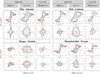 |
Fig. D.1. Same as in Fig.6 but for the disk Opuntia and Lantana, the merger Fuchsia and the disturbed disk Freesia at 60 deg. For each galaxy, from left to right the high S/N ALMA mock data at high- and low-angular resolutions and the Low S/N ALMA mock at medium-angular resolution are shown. |
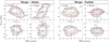 |
Fig. D.2. Same as in Fig. D.1 but for the merger Adenia and Fuchsia at 30 and 80 deg, respectively. The high S/N ALMA mock data at low-angular resolutions are shown. |
All Tables
Summary of the application of the classification techniques on our sample of mock data.
Number of independent resolution elements, NIRE, per galaxy side along the semi-major axis computed as described in Appendix A.
All Figures
|
Fig. 1. Physical properties of the parent and selected sample. The gray stars show the position of EoR galaxies from the SERRA suite (see Pallottini et al. 2022; Kohandel et al., in prep.) in the SFR-M⋆ (left panel), size-M⋆ (medium panel), L[CII]-SFR (right panel) planes. The squares and circles show the selected disks and mergers, respectively, color-coded with the names as indicated by the color-bar. The green diamond shows the disturbed disk Freesia. |
| In the text | |
|
Fig. 2. Sample of SERRA galaxies adopted in this work. For each galaxy we plot the stellar surface density (Σ⋆, upper panels) and the [C II] line surface brightness (Σ[CII], lower panels) for an inclination of 60 degrees. The field of view has a size of 8 kpc. See Table 1 for the main properties of the galaxies. |
| In the text | |
|
Fig. 3. Moment-0 (upper panels), 1 (medium panels), and 2 (bottom panels) for the disk Petunia at 60 deg obtained from the simulated cube (Col. 1) and the mock cubes described at points a) – d) in Sect. 4 (Cols. 2–7) at different angular resolutions (the beam is shown in the bottom left corner as the gray ellipse). In the mock moment-0 maps, the white contours are at 2 and 10 times the rms noise and the color bars are in units of 10 mJy pixel−1 km s−1 in the first column and 100 mJy beam−1 km s−1 for the mock observations. |
| In the text | |
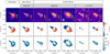 |
Fig. 4. Same as in Fig. 3 but for the merging system Adenia at 60 deg. |
| In the text | |
|
Fig. 5. Three representative spectral channels at velocities 180, 0, −180 km s−1, for the disk Petunia (upper panels) and the merger Adenia (bottom panels) at 60 deg. The left and right subfigures show the high S/N ALMA mock data at high and low-angular resolution. For each subfigure: the upper row shows the data (black contours) and the 3DBAROLO model (red contours). The contour levels are at 2.5, 5, 10 times the rms noise per channel. The gray ellipses in the first panels denote the synthetized beam of the observations. The bottom row shows the residuals normalized to the rms noise. |
| In the text | |
|
Fig. 6. Position-velocity diagrams along the kinematic major (upper panels) and minor axis (bottom panels) for the disk Petunia at 60 deg. The horizontal axis shows the offset from the galaxy center, and the vertical axis represents the line-of-sight velocity centred at the systemic velocity of the galaxy. From left to right, the high S/N ALMA mock data at high-, medium- and low-angular resolutions are shown. The black and red contours show the data and the 3DBAROLO model, respectively. The level contours are at −2.5, 2.5, 5 and 10 times the rms noise. The orange circles show the best-fit rotation velocities (not corrected for inclination) derived using 3DBAROLO. |
| In the text | |
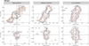 |
Fig. 7. Same as in Fig. 6 but for the merging system Adenia at 60 deg. |
| In the text | |
|
Fig. 8. Relative errors of the recovered rotation velocities (upper panel) and velocity dispersions (bottom panel), computed using Eqs. (2) and (3) for the disturbed disks Freesia (diamonds) and the three disks (squares) of our sample as a function of resolution (number of independent resolution elements along the semi-major axis). Markers with the same color show the mock data for the same galaxy as indicated by the color-bar. The filled and empty markers show the errors for the rotation velocities and velocity dispersions obtained with 3DBAROLO (forward-modeling) and with the velocity-gradient beam-smearing correction. The gray areas mark the 25 percentage. |
| In the text | |
|
Fig. 9. V/σ ratio as a function of resolution (number of independent resolution elements along the semi-major axis) for the disks and the disturbed disk (upper panel) and the mergers (bottom panel). Markers with the same color show the mock data for the same SERRA galaxy as indicated by the color-bar. The black dashed line shows the threshold at 1.8. The filled markers show the V/σ ratios obtained with 3DBAROLO that is a 3D forward-modeling approach is applied to correct for the beam-smearing effect. The empty markers show the V/σ obtained when a velocity-gradient method is employed to correct for the beam-smearing effect. |
| In the text | |
|
Fig. 10. Fraction of mergers classified as disks based on the criteria described in Sects. 6.1 (left, red bars) and 6.2 (right) as a function of resolution. In the left panel, the light blue and dark green bars show the fraction of galaxies with smooth velocity maps and V/σ ≳ 1.8. The latter are obtained using the velocity-gradient method for correcting for beam smearing. The non-zero fraction at NIRE ∼ 7.5 is due to the low S/N mock data. In the right panel, we show the fractions obtained using the Shapiro et al. (2008) and Bellocchi et al. (2012) methods as green and orange bars, respectively. Using the classification method described in Sect. 6.1, the only non-zero fraction of misclassified disks is obtained for NIRE ≲ 2 when the velocity-gradient method is used for correcting for beam smearing. In this case, 50% of disks are classified as dispersion-dominated systems. Using the kinemetry-based method all disks are correctly classified. |
| In the text | |
|
Fig. 11. Global asymmetric parameters as a function of resolution for the disks (squares), mergers (circles), and the disturbed disk Freesia (diamonds). The global asymmetric parameters are computed according to the definitions of Shapiro et al. (2008) (upper) and Bellocchi et al. (2012) (bottom). The solid black and dashed gray lines in the upper panel show the limit of 0.5 and 0.14, indicated by Shapiro et al. (2008) and Bellocchi et al. (2016) as the thresholds for distinguishing between disks and mergers, respectively. In the bottom panel, the solid and dashed black lines show the limits of 0.19 and 0.16, indicated by Bellocchi et al. (2016) as the discriminators between disks and mergers at low and high-z, respectively. |
| In the text | |
|
Fig. 12. Kinematic maps and profile for the barely resolved ALMA mock data for the disk Opuntia at 30 (upper panels), 60 (medium panels) and 80 deg (bottom panels). Column 1: [C II] integrated spectrum (gray histogram) and best-fit model (solid green line), resulting from the sum of two components (red dashed and purple dotted lines). Column 2: moment-0 map with black contours showing the 3, 6 and 9 rms levels. Columns 3 and 4: moment-1 and moment-2 maps obtained following the methodology in Romano et al. (2021) (see Sect. 6.3 for details). The dashed lines in the moment-1 map show the directions of the major and minor axis along which the PV-diagrams are extracted. Columns 5 and 6: PV diagrams along the major (left) and minor (right) axis with contours at −2 rms (dashed gray lines) and 2, 4, 8 rms (solid black lines). |
| In the text | |
|
Fig. 13. Same as in Fig. 12, but for the disturbed disk Freesia and the merging systems Adenia, Fuchsia at i = 60 deg. |
| In the text | |
|
Fig. 14. Schematic representation of the morphological and symmetrical features in the major axis PV diagrams considered for the computation of the P parameters defined in Sect. 7.1. Left panel: PV diagram for a representative thin rotating disk model along the major axis. The dotted gray horizontal line shows the position of the systemic velocity that divides the major-axis PV diagram into regions A1 and A2, while the dotted gray vertical lines indicate the center dividing A1 and A2 into two regions, l and r. The ith representative pixels used for the computation of Pmajor are shown in the regions A1 and A2, respectively. The blue dotted contours enclose the 20% brightest pixels, and the yellow crosses are their flux-weighted centroids. The black plus indicates the outermost radius used for the extraction of the kinematic parameters, and the solid orange lines are Vlos, out, the average values of the galaxy line-of-sight velocities. The double arrow indicates ΔV, the extension along the velocity axis for one of the peak distributions. The major-axis PV diagrams from the high S/N, low-resolution mock data of the disk Lantana and merger Adenia are shown in the central and right panels. |
| In the text | |
|
Fig. 15. PV parameters described in Sect. 7.1 as a function of the independent resolution elements along the semi-major axis (Appendix A for details). |
| In the text | |
|
Fig. 16. Importance of the different PV parameters for the disk/merger classification. The fractional importance is computed for the different parameters (definitions in Sect. 7.1) by constructing a decision tree classifier to distinguish between disks and mergers. The decision tree uses our sample of 84 galaxies with different resolutions and S/N, using 70% (30%) of the data for training (testing), resulting in a R2 score of 84%. |
| In the text | |
|
Fig. 17. Position of the 84 mock data (squares: disks, circles: mergers; diamonds: disturbed disk Freesia) in the PVsplit parameter space. The empty black square and circle show the position of a spiral and a merger galaxy at z = 0, respectively. A movie with a 3D visualization of this figure is available online. |
| In the text | |
|
Fig. D.1. Same as in Fig.6 but for the disk Opuntia and Lantana, the merger Fuchsia and the disturbed disk Freesia at 60 deg. For each galaxy, from left to right the high S/N ALMA mock data at high- and low-angular resolutions and the Low S/N ALMA mock at medium-angular resolution are shown. |
| In the text | |
|
Fig. D.2. Same as in Fig. D.1 but for the merger Adenia and Fuchsia at 30 and 80 deg, respectively. The high S/N ALMA mock data at low-angular resolutions are shown. |
| In the text | |
Current usage metrics show cumulative count of Article Views (full-text article views including HTML views, PDF and ePub downloads, according to the available data) and Abstracts Views on Vision4Press platform.
Data correspond to usage on the plateform after 2015. The current usage metrics is available 48-96 hours after online publication and is updated daily on week days.
Initial download of the metrics may take a while.