| Issue |
A&A
Volume 667, November 2022
|
|
|---|---|---|
| Article Number | A1 | |
| Number of page(s) | 25 | |
| Section | Planets and planetary systems | |
| DOI | https://doi.org/10.1051/0004-6361/202243093 | |
| Published online | 28 October 2022 | |
The HD 93963 A transiting system: A 1.04 d super-Earth and a 3.65 d sub-Neptune discovered by TESS and CHEOPS★
1
Dipartimento di Fisica, Università degli Studi di Torino,
via Pietro Giuria 1,
10125
Torino, Italy
e-mail: This email address is being protected from spambots. You need JavaScript enabled to view it.
2
Aix Marseille Univ., CNRS, CNES, LAM,
38 rue Frédéric JoliotCurie,
13388
Marseille, France
3
Department of Astronomy, Stockholm University, AlbaNova University Center,
10691
Stockholm, Sweden
4
Physikalisches Institut, University of Bern,
Gesellsschaftstrasse 6,
3012
Bern, Switzerland
5
Instituto de Astrofisica e Ciencias do Espaco, Universidade do Porto, CAUP,
Rua das Estrelas,
4150-762
Porto, Portugal
6
Instituto de Astrofisica de Canarias,
38200
La Laguna, Tenerife, Spain
7
Dept. Astrofísica, Universidad de La Laguna (ULL),
38206
La Laguna, Tenerife, Spain
8
NASA Exoplanet Science Institute – Caltech/IPAC,
1200 E. California Blvd,
Pasadena, CA
91125, USA
9
Space Science and Astrobiology Division NASA Ames Research Center,
M/S 245-6,
Moffett Field, CA
94035, USA
10
Center for Space and Habitability,
Gesellsschaftstrasse 6,
3012
Bern, Switzerland
11
Observatoire Astronomique de l’Université de Genève,
Chemin Pegasi 51,
Versoix, Switzerland
12
Department of Astronomy, Stockholm University,
106 91
Stockholm, Sweden
13
Space Research Institute, Austrian Academy of Sciences,
Schmiedlstrasse 6,
8042
Graz, Austria
14
Lund Observatory, Dept. of Astronomy and Theoretical Physics, Lund University,
Box 43,
22100
Lund, Sweden
15
Centre for Exoplanet Science, SUPA School of Physics and Astronomy, University of St Andrews,
North Haugh,
St Andrews
KY16 9SS, UK
16
Department of Physics and Kavli Institute for Astrophysics and Space Research, Massachusetts Institute of Technology,
Cambridge, MA
02139, USA
17
Department of Physics, Shahid Beheshti University,
Tehran, Iran
18
Laboratoire J.-L. Lagrange, Observatoire de la Côte d’Azur (OCA), Université de Nice-Sophia Antipolis (UNS), CNRS,
Campus Valrose,
06108
Nice Cedex 2, France
19
Leiden Observatory, University of Leiden,
PO Box 9513,
2300 RA
Leiden, The Netherlands
20
Department of Space, Earth and Environment, Chalmers University of Technology, Onsala Space Observatory,
43992
Onsala, Sweden
21
Stellar Astrophysics Centre, Department of Physics and Astronomy, Aarhus University,
Ny Munkegade 120,
8000
Aarhus C, Denmark
22
Nordic Optical Telescope,
Rambla José Ana Fernández Pérez 7,
38711
Breña Baja, Spain
23
Center for Astrophysics | Harvard & Smithsonian,
60 Garden Street,
Cambridge, MA
02138, USA
24
Institute of Planetary Research, German Aerospace Center (DLR),
Rutherfordstrasse 2,
12489
Berlin, Germany
25
Rheinisches Institut für Umweltforschung an der Universität zu Köln,
Aachener Strasse 209,
50931
Köln, Germany
26
Institut de Ciencies de l’Espai (ICE, CSIC),
Campus UAB, Can Magrans s/n,
08193
Bellaterra, Spain
27
Institut d’Estudis Espacials de Catalunya (IEEC),
08034
Barcelona, Spain
28
Admatis,
5. Kandó Kálmán Street,
3534
Miskolc, Hungary
29
Depto. de Astrofisica, Centro de Astrobiología (CSIC-INTA),
ESAC campus,
28692
Villanueva de la Canada, Madrid, Spain
30
Departamento de Fisica e Astronomia, Faculdade de Ciencias, Universidade do Porto,
Rua do Campo Alegre,
4169-007
Porto, Portugal
31
Harvard-Smithsonian Center for Astrophysics,
60 Garden Street, P-333,
MS-16,
Cambridge, MA
02138, USA
32
Université Grenoble Alpes, CNRS, IPAG,
38000
Grenoble, France
33
NASA, Goddard Space Flight Center,
8800 Greenbelt Rd,
Greenbelt, MD
20771, USA
34
Université de Paris, Institut de physique du globe de Paris, CNRS,
75005
Paris, France
35
Centre for Mathematical Sciences Lund University,
Box 118,
SE 221 00
Lund, Sweden
36
Astrobiology Research Unit, Université de Liège,
Allée du 6 Août 19C,
4000
Liège, Belgium
37
Space sciences, Technologies and Astrophysics Research (STAR) Institute, Université de Liège,
Allée du 6 Août 19C,
4000
Liège, Belgium
38
University of California at Santa Cruz,
Santa Cruz, CA, USA
39
Komaba Institute for Science, The University of Tokyo,
3-8-1 Komaba, Meguro,
Tokyo
153-8902, Japan
40
Instituto de Astrofísica de Canarias (IAC),
38205
La Laguna, Tenerife, Spain
41
Astronomical Institute, Slovak Academy of Science, Stellar Department, Tatranská Lomnica,
05960
Vysoké Tatry, Slovakia
42
ELTE Eötvös Lorând University, Gothard Astrophysical Observatory,
9700
Szombathely,
Szent Imre h. u. 112,
Hungary
43
MTA-ELTE Exoplanet Research Group,
9700
Szombathely,
Szent Imre h. u. 112,
Hungary
44
MTA-ELTE Lendület Milky Way Research Group,
9700
Szombathely,
Szent Imre h. u. 112,
Hungary
45
University of Vienna, Department of Astrophysics,
Türkenschanzstrasse 17,
1180
Vienna, Austria
46
Institut d’astrophysique de Paris, UMR7095 CNRS, Université Pierre & Marie Curie,
98bis boulevard Arago,
75014
Paris, France
47
Observatoire de Haute-Provence, CNRS, Université d’Aix-Marseille,
04870
Saint-Michel-l’Observatoire, France
48
Department of Physics, University of Warwick,
Gibbet Hill Road,
Coventry
CV4 7AL, UK
49
Science and Operations Department – Science Division (SCI-SC), Directorate of Science, European Space Agency (ESA), European Space Research and Technology Centre (ESTEC),
Keplerlaan 1,
2201-AZ
Noordwijk, The Netherlands
50
NASA Ames Research Center,
Mail Stop 269-3,
Bldg. T35A, Rm. 102,
PO Box 1,
Moffett Field, CA
94035-0001, USA
51
Konkoly Observatory, Research Centre for Astronomy and Earth Sciences,
1121
Budapest,
Konkoly Thege Miklós út 15-17,
Hungary
52
IMCCE, UMR8028 CNRS, Observatoire de Paris, PSL Univ.,
Sorbonne Univ., 77 av. Denfert-Rochereau,
75014
Paris, France
53
INAF, Osservatorio Astronomico di Padova,
Vicolo dell’Osservatorio 5,
35122
Padova, Italy
54
Astrophysics Group, Keele University,
Staffordshire
ST5 5BG, UK
55
Astrobiology Center,
2-21-1 Osawa,
Mitaka, Tokyo
181-8588, Japan
56
Department of Astrophysics, University of Vienna,
Tuerkenschanzstrasse 17,
1180
Vienna, Austria
57
INAF, Osservatorio Astrofisico di Catania,
Via S. Sofia 78,
95123
Catania, Italy
58
Citizen Scientist, Marica,
Rio de Janeiro, Brazil
59
Institute of Optical Sensor Systems, German Aerospace Center (DLR),
Rutherfordstrasse 2,
12489
Berlin, Germany
60
Dipartimento di Fisica e Astronomia “Galileo Galilei”, Universita degli Studi di Padova,
Vicolo dell’Osservatorio 3,
35122
Padova, Italy
61
ETH Zurich, Department of Physics,
Wolfgang-Pauli-Strasse 27,
8093
Zurich, Switzerland
62
Cavendish Laboratory,
JJ Thomson Avenue,
Cambridge
CB3 0HE, UK
63
ESTEC, European Space Agency,
2201 AZ
Noordwijk, The Netherlands
64
Center for Astronomy and Astrophysics, Technical University Berlin,
Hardenberstrasse 36,
10623
Berlin, Germany
65
Institut für Geologische Wissenschaften, Freie Universität Berlin,
12249
Berlin, Germany
66
Royal Astronomical Society,
Burlington House, Piccadilly,
London
W1J 0BQ, UK
67
Department of Earth, Atmospheric and Planetary Sciences, Massachusetts Institute of Technology,
Cambridge, MA
02139, USA
68
Department of Aeronautics and Astronautics, MIT,
77 Massachusetts Avenue,
Cambridge, MA
02139, USA
69
SETI Institute/NASA Ames Research Center,
339 Bernardo Ave, Suite 200,
Mountain View, CA
94043, US
70
Institute of Astronomy, University of Cambridge,
Madingley Road,
Cambridge
CB3 0HA, UK
Received:
12
January
2022
Accepted:
19
June
2022
Abstract
We present the discovery of two small planets transiting HD 93963A (TOI-1797), a GOV star (M* = 1.109 ± 0.043M⊙, R* = 1.043 ± 0.009 R⊙) in a visual binary system. We combined TESS and CHEOPS space-borne photometry with MuSCAT 2 ground-based photometry, ‘Alopeke and PHARO high-resolution imaging, TRES and FIES reconnaissance spectroscopy, and SOPHIE radial velocity measurements. We validated and spectroscopically confirmed the outer transiting planet HD 93963 A c, a sub-Neptune with an orbital period of Pc ≈ 3.65 d that was reported to be a TESS object of interest (TOI) shortly after the release of Sector 22 data. HD 93963 A c has amass of Mc = 19.2 ± 4.1 M⊕ and a radius of Rc = 3.228 ± 0.059 R⊕, implying a mean density of ρc = 3.1 ± 0.7 g cm-3. The inner object, HD 93963 A b, is a validated 1.04 d ultra-short period (USP) transiting super-Earth that we discovered in the TESS light curve and that was not listed as a TOI, owing to the low significance of its signal (TESS signal-to-noise ratio ≈6.7, TESS + CHEOPS combined transit depth Db = 141.5−8.3+8.5 ppm). We intensively monitored the star with CHEOPS by performing nine transit observations to confirm the presence of the inner planet and validate the system. HD 93963 A b is the first small (Rb = 1.35 ± 0.042 R⊕) USP planet discovered and validated by TESS and CHEOPS. Unlike planet c, HD 93963 Ab is not significantly detected in our radial velocities (Mb = 7.8 ± 3.2 M⊕). The two planets are on either side of the radius valley, implying that they could have undergone completely different evolution processes. We also discovered a linear trend in our Doppler measurements, suggesting the possible presence of a long-period outer planet. With a V-band magnitude of 9.2, HD 93963 A is among the brightest stars known to host a USP planet, making it one of the most favourable targets for precise mass measurement via Doppler spectroscopy and an important laboratory to test formation, evolution, and migration models of planetary systems hosting ultra-short period planets.
Key words: planets and satellites: detection / planets and satellites: fundamental parameters / instrumentation: photometers / instrumentation: spectrographs / methods: data analysis
Tables of DRS and PIPE extracted lightcurves and detrended data are only available at the CDS via anonymous ftp to cdsarc.u-strasbg.fr (130.79.128.5) or via http://cdsarc.u-strasbg.fr/viz-bin/cat/J/A+A/667/A1
© L. M. Serrano et al. 2022
 Open Access article, published by EDP Sciences, under the terms of the Creative Commons Attribution License (https://creativecommons.org/licenses/by/4.0), which permits unrestricted use, distribution, and reproduction in any medium, provided the original work is properly cited.
This article is published in open access under the Subscribe-to-Open model. This email address is being protected from spambots. You need JavaScript enabled to view it. to support open access publication.
1 Introduction
Following the discovery of the first planet orbiting a solar-like star (51 Peg b; Mayor & Queloz 1995), the field of exoplanets has continuously evolved at a fast pace, moving from the mere exploratory objective of finding new planets, to the aim of measuring their radii and masses and, when possible, of detecting and characterizing their atmospheres. This transition has been possible thanks to high-precision ground-based facilities, such as High Resolution Echelle Spectrometer (HIRES, Vogt et al. 1994), High Accuracy Radial velocity Planet Searcher (HARPS, Mayor et al. 2003), High Accuracy Radial velocity Planet Searcher for the Northern emisphere (HARPS-N, Cosentino et al. 2012), Echelle SPectrograph for Rocky Exoplanets and Stable Spectroscopic Observations (ESPRESSO, Pepe et al. 2021), and space-based missions such as Convection, Rotation et Transits planétaires (CoRoT, Baglin et al. 2006), Kepler (Borucki et al. 2010), Kepler-2 (K2, Howell et al. 2014), and, most recently, Transiting Exoplanet Survey Satellite (TESS Ricker et al. 2015). Data analysis techniques have also improved, providing an enhanced capability to disentangle the signature of an orbiting planet from the spectroscopic and photometric signals induced by stellar activity (e.g. Hatzes et al. 2011; Haywood et al. 2014; Serrano et al. 2018; Hippke & Heller 2019; Luque et al. 2021).
Statistical analyses on the population of exoplanets thus far discovered have shown that about 25–30% of Sun-like stars in our Galaxy host super-Earths (RP = 1–2 R⊕, MP = 1–10 M⊕) and sub-Neptunes (RP = 2–4 R⊕, MP = 10–40 M⊕) in tightly packed systems with orbital periods shorter than 100 d (see, e.g. Silburt et al. 2015; Mulders et al. 2016). One of the biggest surprises was the discovery of a population of exotic planets with orbital periods Porb ≲ 1 d, the so-called ultra-short period (USP) planets. With the exception of a small subgroup of giant planets (see, e.g. Sahu et al. 2006) and a couple of Neptune-sized objects (e.g. TOI-849 b and TOI-193 b; Armstrong et al. 2020; Jenkins et al. 2020), most of the known USP planets are Earth-like objects or super-Earths (RP < 2 R⊕), with CoRoT-7 b being the prototype of this class of objects (Léger et al. 2009).
Launched in December 2019, the CHaracterizing ExOPlanet Satellite (CHEOPS; Benz et al. 2021) is the first ESA small-class mission whose main goal is to perform high-precision photometry of bright stars (V < 12) known to host planets. CHEOPS is pursuing a variety of science goals, both in exoplanetary and stellar physics (some references, Lendl et al. 2020; Leleu et al. 2021; Van Grootel et al. 2021; Delrez et al. 2021; Borsato et al. 2021; Morris et al. 2021; Swayne et al. 2021; Szabó et al. 2021). The mission is also discovering new transiting planets, such as HD 108236 f (Bonfanti et al. 2021a) and TOI-178b, c, and f (Leleu et al. 2021).
To help the community arrange follow-up observations and report the detection of TESS exoplanets, specific systems that pass through a validation process attain the status of TESS objects of interest (TOIs). As a first step, the process confirms that the signal is real and astrophysical. Then, it performs a Bayesian model comparison with other astrophysical signals to show that the planetary hypothesis is overwhelmingly preferred. Finally, only transit events that surpass the signal-to-noise ratio S/N ~ 7.1 threshold are upgraded to the status of candidates and receive a TOI number (see Guerrero et al. 2021, for further details). Some transit-like signals may not pass the validation process for various reasons. Simple examples may be single transits or two transits with a significant depth mismatch, as in the case of ν2 Lupib and c. Although the two planets already appeared transiting in TESS Sector 12, the star received a TOI number only one year after, when the data were visually inspected (Kane et al. 2020). Another case of non-detection by the TESS pipeline involves small planets, which can generate shallow transit-like signals with S/N< 7.1. Since small planets are common and the S/N threshold has been chosen to minimize the false alarm rate (Jenkins et al. 2016a), there may be transiting exoplanets not being identified and followed up, even if they are part of systems where TOIs have already been assigned.
The confirmation of less significant transit signals may be performed through other means, such as radial velocity (RV) follow-up observations of the star (see, as an example, TOI-421; Carleo et al. 2020). However, using Doppler spectroscopy to confirm a planet may be time-consuming. Transiting planet candidates with low significant transit signals in TESS light curves can be efficiently vetted against false alarm detections by performing space-based photometric follow-up observations of the predicted transits with a more precise instrument.
Within the CHEOPS Guaranteed Time Observation (GTO) programme, we perform CHEOPS photometric follow-up observations of mostly bright (V < 11) TOIs with the immediate objective of identifying additional small planet candidates. This is done by performing high-precision photometry of transiting planet candidates with a non-significant transit detection in TESS light curves (S/N < 7.1). As transiting planet candidates in multiple systems have a much lower probability of being false positives (Latham et al. 2011), we mainly focus on low S/N non-TOI candidates in systems known to host at least one TOI candidate. Identifying new non-TOIs orbiting a TOI target opens up the possibility of increasing both the number of known multi-planet systems, and the number of planets in an already known multi-planet system. Furthermore, by construction, this programme delivers viable targets for RV follow-up campaigns and improved transit parameters and ephemerides.
As part of CHEOPS GTO programs CHEOPS Objects of Interest (CHOI, PR110045) and CHESS (PR110031), we photometrically monitored the brightest component of the visual binary HD 93963, also known as TOI-1797 (Table 1). HD 93963 A is a bright (V = 9.2) G0 V, nearby (82 pc) star found to host a 3.65 d sub-Neptune candidate, which was reported as likely being a planet in Giacalone et al. (2021) with the name TOI-1797.01. We independently searched the TESS light-curve for possible candidates, and identified an additional transit signal with a period of 1.04 d that was not included in the TOI candidates list due to its low S/N ~ 6.7. Here, we report on the discovery of this additional ultra short-period transiting planet, as well as the validation and radius determination of both bodies. This result was made possible thanks to the photometric observations carried out with CHEOPS. With its high precision and high scheduling flexibility CHEOPS was the only instrument capable of clearly detecting the transit signal induced by the 1.04d planet, making HD 93963A the first system with an ultra-short period planet discovered and validated by CHEOPS.
The present paper is organized as follows. In Sect. 2, we present the TESS data and our independent search for transit signals. Section 3 briefly describes the CHEOPS mission and presents the strategy of our observations and the data reduction. Section 4 presents the high-resolution imaging observations of HD 93963 A and its stellar companion HD 93963 B. Section 5 presents the spectra used for the stellar characterization (Sect. 6). Section 7 is dedicated to the analysis of the TESS and CHEOPS light curves and the determination of the parameters of HD 93963 A b and c. The validation of both planets is discussed in Sect. 8. In Sect. 9, we report the analysis of SOPHIE RV follow-up data and the measurement of HD 93963 A c mass. Section 10 describes the planetary system orbiting HD 93963 A, with empirical estimates of the masses of the two discovered planets and it discusses some of the possible migration theories that may be relevant to our system. In this section, we also present the importance and the impact of our discovery on future science.
2 TESS observations
2.1 Data collection
TESS observed HD 93963 A in Sector 22, during year 2 of its nominal mission, from 18 February to 18 March 2020, with data from the target stacked and telemetered at 2-min cadence. The space telescope monitored the star using camera #1 and CCD #3 (each CCD has a field of view of FoV= 12° × 12°; Ricker et al. 2015). In addition to a 1 day gap due to the data downlink during perigee passage, the TESS observations of HD 93963 A were affected by significant moon-light contamination, resulting in the removal of 2 additional days of data at the beginning of each half sector. Overall, a total of 5 d of data was removed from the Sector. The TESS target pixel files were processed and calibrated by the Science Processing Operation Center (SPOC; Jenkins et al. 2016b) at the NASA Ames Research Center. The light curve was extracted using simple aperture photometry (SAP; Twicken et al. 2010; Morris et al. 2020) and processed using the Presearch Data Conditioning (PDC) algorithm, which uses a Bayesian maximum a posteriori approach to remove the majority of instrumental artefacts and systematic trends (Smith et al. 2012; Stumpe et al. 2012, 2014). We retrieved the PDC-SAP TESS light curve of HD 93963 A from the Mikulski Archive for Space Telescope (MAST1; see the upper panel of Fig. 1).
The SPOC team searched the PDC-SAP light curve for transit-like signals, using a pipeline that iteratively performs multiple transiting planet searches and stops when it fails to find subsequent transit-like signatures above the detection threshold of S/N ~ 7.1. On 28 March 2020, SPOC published the results in the Data Validation Report (DVR; Twicken et al. 2018; Li et al. 2019). The TESS vetting team at the Massachusetts Institute of Technology (MIT) inspected the DVR to review the Threshold Crossing Events (TCEs), and later announced the detection of a transiting planetary candidate (TOI 1797.01, Guerrero et al. 2021) with a period of Porb ≈ 3.65 d, a depth of about 800 ppm, and a duration of T14 ≈ 2.0 h. The candidate passed all the automatic validation tests from the TCE, such as odd-even transit depth variation and ghost diagnostic tests.
Main identifiers, equatorial coordinates, optical and infrared magnitudes, and the fundamental parameters of HD 93963 A.
2.2 Independent transit search
In order to confirm the presence of the 3.65 d TOI announced by the TESS team and look for additional planet candidates, we independently searched the PDC-SAP TESS light-curve for transit signals. In order to do so, we applied different detrending algorithms and methodologies as described below.
Method 1
We filtered out the variability of the light-curve using the Savitzky-Golay method (Savitzky & Golay 1964; Press et al. 2002) and applied the Détection Spécialisé de Transits (DST; Cabrera et al. 2012), which searches for transits using a parabolic function as a transit model. In addition to the detection algorithm, we also used the information retrieved from the TESS data release notes and DVR, to assess and remove signals arising from possible astrophysical false positives or systematics.
Method 2
We modelled the stellar activity modulation using the Gaussian Process (GP) implemented within the public code citlalicue (Barragán et al. 2022). Briefly, the routine masks out the planetary transits and bins the data using 3 h bins. It performs an iterative maximum likelihood optimization coupled with a 5-sigma clipping algorithm, in order to fit a GP with quasi-periodic kernel and remove possible outliers. To maximize the performance of citlalicue, we masked out the transits of the 3.65 d planet, as they can affect the modelling of the stellar activity signal. We flattened the light curve, dividing the full PDC-SAP time series (including the data points previously masked out) by the retrieved correlation model and we searched the TESS detrended light curve for transits, by repeatedly applying the Transit Least Square algorithm (TLS, Hippke & Heller 2019). TLS performs a least square minimization on the entire non binned light-curve, modelling the transit with a quadratic limb darkening law, as described in Mandel & Agol (2002).
Method 3
We used an out-of-box polynomial fit (which by its nature leaves transits untouched) to remove variability from the light curve. Then, as in the case of Method 2, we iteratively performed a TLS periodic search and masked the detected transit events, until no significant signal remained.
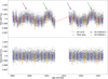 |
Fig. 1 TESS light curve of HD 93963 A. In-transit data points of the 3.65 d and the 1.04 d candidate are marked in yellow and blue, respectively. Upper panel: PDC-SAP flux (grey) and detrending model (red), as obtained with citlalicue (Sect. 2.2). The arrows point to the repeated maxima we identified in the light curve: the purple arrows points to the maximum at ~1905 (BJD-2457000) and at its repetition at ~1918 (BJD-2457000). The green arrows point to the second maxima, that appears at ~1911 (BJD-2457000) and at ~1924 (BJD-2457000). Lower panel: detrended flux. |
Method 4
We applied the detection pipeline EXOTRANS to the TESS light curve. EXOTRANS removes discontinuities and stellar variability with the wavelet-based filter VARLET (Grziwa et al. 2016), and routinely searches for transits applying an advanced version of the Box Least-Squares algorithm (BLS; Kovács et al. 2016). EXOTRANS can detect multiple transit signals and-or transits masked by other strong periodic events (such as systematics, background binaries).
Each of the four different methods confirmed the 3.65 d transit candidate announced by the TESS team and unveiled the presence of a possible additional transit signal with a period of 1.04 d, a depth of ~140 ppm, and a duration of ~2 h. This transit has a S/N ~ 6.7, which is below the detection threshold adopted by the TESS team (S/N ~ 7.1). We thus focused our efforts on understanding the nature of this signal performing further photometric observations and complementary high-resolution imaging and Doppler spectroscopy.
3 CHEOPS observations
In order to confirm the transit signal at 1.04 d, validate the planetary system, and precisely determine the radius of the two planets, we performed CHEOPS photometric follow-up observations of HD 93963 A between February and April 2021. We started by verifying whether we could detect the additional planet candidate at 1.04 d. A modelling of TESS transits2 provided the following ephemeris: P = 1.03897 ± 0.00035 d and T0(BJD3) = 2458901.279 ± 0.004 d. Due to the relatively short baseline of the TESS light curve (~28 d) and the low significance of our detection (S/N ≈ 6.7), the propagated uncertainty on the predicted time of transit in February 2021 (nearly one year after the TESS observations) amounted to ~3 h. Given the short orbital period of the candidate (1.04 d), we decided to follow a conservative approach and continuously observe HD 93963 A for nearly 1.3 d4, centring our observations around the transit that was expected to occur on 07 February 2021 (UTC). Taking into account the transit duration (~2 h), this would have allowed us to cover at least one full transit, regardless of the uncertainties on the transit time, while having a long out-of-transit baseline to properly detrend the data.
Figure 2 shows the raw CHEOPS light curve of the first visit of HD 93963 A. The gaps in the time series are due to the Earth’s occultation and the passage of the spacecraft above the South Atlantic Anomaly (SAA)5. A visual inspection of the light curve revealed the presence of a transit-like feature with a duration and depth compatible with those of the transits observed by TESS and occurring ~ 1 h after the predicted time of mid-transit. We jointly modelled the TESS and CHEOPS light curve following the same methods described in Sect. 7 and refined the period (P= 1.0391581 ± 0.0000387 d).
With one single CHEOPS visit we ‘upgraded’ the 1.04 d signal to planetary candidate and improved the precision on its period estimate by one order of magnitude. We decided to keep observing the candidate, scheduling seven shorter CHEOPS visits of the 1.04 d transit candidate and stopped the follow-up when we reached a precision on the planetary radius of ~3%. For the sake of completeness, we also observed one transit of the 3.65 d TOI candidate and verified the achromaticity of the event. The observations were performed with a global efficiency (duty cycle) higher than 50%. Table 2 reports the starting and ending time of each CHEOPS visit, along with the number of data points.
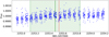 |
Fig. 2 Raw data points of the first CHEOPS visit (blue circles). The transit of the 1.04 d planet is visible at the centre of the visit. The mid-transit time, as predicted by the TESS ephemeris, is highlighted with a vertical green line, while the area coloured in light green is the corresponding 3 σ interval of confidence. The mid-transit time predicted with the ephemeris in the third column of Table 5 is marked with a vertical red line. The time difference between the red and the green lines is ~1 h. |
List of CHEOPS observations for HD 93963 A with start and end date, number of data points, and terms used to decorrelate the respective light curves using pycheops.
3.1 CHEOPS data reduction
CHEOPS data for each visit is downlinked to the ground as packages of circular images with a diameter of 200 px centred around the target star. Those images, referred to as “subarrays”, are small windows of the CHEOPS CCD, whose sky-projected area has a diameter of about 200″, which corresponds to ~4% of the full CHEOPS field of view (FoV). The subarrays were automatically processed with the latest version of the Data Reduction Pipeline (DRP; Hoyer et al. 2020), DRP ν13, which includes bias and dark subtraction, non-linearity and flat field correction. In addition, the DRP corrects for sky-background, cosmic-ray hits, and smearing trails of nearby stars. The DRP performs aperture photometry on the processed CHEOPS images using different circular masks centred around the target. The mask follows the movements of the star due to the spacecraft pointing jitter and telescope rolling around the optical axis, which ensures a thermally stable environment of the payload radiators. The circular photometric masks can have three different standard sizes, namely, the RINF, DEFAULT, and RSUP apertures with radii of 22.5, 25.0, 30.0 pixels, respectively. In addition, the DRP also extracts the photometric flux using an OPTIMAL aperture which radius is estimated independently for single visits. The OPTIMAL aperture is intended to minimize the instrumental noise and contamination level from nearby stars. The DRP extraction provides the user with a series of vectors that allow one to model instrumental and environmental effects. Users can retrieve from the data the orbital roll-angle ϕ of the telescope, the x and y position in the CCD of the centre of the target’s point spread function (PSF), the estimated sky background level, the smear curve, and the contamination by PSFs of background stars (please refer to Hoyer et al. 2020, for additional details on how the contamination is treated by the DRP).
We also extracted PSF photometry on the CHEOPS images, using the python module6 PIPE (Brandeker et al., in prep.). Point-spread function photometry has the advantage of being less sensitive to contaminants than aperture photometry, which makes it particularly well suited for crowded fields or when there is a suspected contaminant. In addition, with PIPE we can also remove the smear effect in advance. We used the observations of HD 93963 A to derive an empirical PSF, used by PIPE to extract the photometry. As such, PIPE provides as output a FITS file that includes the extracted light curve and the same decorrelation vectors provided by the DRP, with the exception of smearing and contamination. The difference in RMS between DRP and PIPE light curves is only ~30 ppm, but as the PSF photometry can better account for the noise due to the closest contaminants, we decided to use PIPE extracted light curves for our analysis.
3.2 CHEOPS light curve detrending
We detrended the nine CHEOPS visits with the code pycheops (Maxted et al. 2022), which allows one to de-correlate the data using the vectors that describe the short-term instrumental photometric trends: roll angle, centroid movements, smear curve, and contamination by background stars. pycheops can also detrend the CHEOPS light curves using simple linear or quadratic trends.
We first applied a 3 σ clipping algorithm as implemented in pycheops to remove outliers from the CHEOPS data and analysed each visit individually to check if it is affected by any of the known CHEOPS instrumental systematics. We excluded from the process the smear and contamination effects, because they are already accounted for by the PIPE extraction. We chose the detrending vectors via a Bayes factor pre-selection method (Trotta 2007), which routinely fits each visit with a least mean square method, accounting for the transit model and one of the possible decorrelation terms. In Table 2, we report those terms for which we obtained a Bayes factor lower than 1. We performed preliminary modelling of the eight CHEOPS visits of the 1.04 d transit signal using Markov chain Monte Carlo simulations implemented in pycheops, including the effects of both the transits and the decorrelation terms listed in Table 2. For the 3.65 d candidate, we applied the same methodology adopted for the visits of the 1.04 d transit signal. We finally flattened the light curves, dividing the data by the inferred model of the instrumental noise. Figures 3 and 4 show the 8 detrended transit light curves of the 1.04 d candidate and the detrended single visit of the 3.65 d candidate, respectively, as observed with CHEOPS.
4 Ground-based photometry and imaging
Stellar companions, projected closely on the sky, whether bound or unbound (such as a faint nearby eclipsing binary (NEB)) can create false positive signals and provide “third-light” that will dilute the transit signal. Unaccounted for “third-light” in a transit fit will cause the derived planet radius to be underestimated (Ciardi et al. 2015) and can even lead to non-detection of small planets (Lester et al. 2021). Given that nearly one-half of solar-like stars are binary (Matson et al. 2018), high-resolution imaging may help avoid incorrect interpretations of any detected exoplanet.
4.1 LCOGT 1m observations
We observed a full transit of HD 93963 c in Pan-STARRS Y -band on UT 2021 January 27 from the Las Cumbres Observatory Global Telescope (LCOGT; Brown et al. 2013) 1.0 m network node at McDonald Observatory in near Fort Davis, Texas. The telescope is equipped with the 4096 × 4096 SINISTRO camera having an image scale of 0.389″ per pixel, resulting in a 26′ × 26′ field of view. The images were calibrated by the standard LCOGT BANZAI pipeline (McCully et al. 2018), and photometric data were extracted using AstroImageJ (Collins et al. 2017). Circular photometric apertures with radius of 9.7″ were used to extract the differential photometry. The target star aperture also includes most of the flux from the companion TIC 368435331, which is the nearest TESS Input Catalog and Gaia EDR3 neighbour and which we refer to as HD 93963 B. We detected a low signal-to-noise, roughly 900 ppt event, having transit timing consistent with the ephemeris derived from the TESS and CHEOPS data presented in this work (see Fig. 5).
4.2 MuSCAT 2 observations
On 21–22 May 2021, HD 93963 A was observed with the MuSCAT 2 multi-colour imager (Narita et al. 2019) mounted at the 1.52 m Telescopio Carlos Sanchez (TCS) of Teide Observatory (Tenerife, Spain). MuSCAT 2 can perform simultaneous photometry in 4 broad passbands, namely, the g (400–550 nm), r (550–700 nm), i (700–820 nm), and zs (820–920 nm) bands. The data calibration and photometric extraction was done using the dedicated MuSCAT 2 pipeline (Parviainen et al. 2019). The observation aimed at verifying that the 1.04 d signal is not caused by a nearby eclipsing binary (NEB). To this purpose, we used the zs and i filters to observe HD 93963 A with 2 and 3 s exposure times, respectively, and the other 2 filters to take 30 s exposures to increase the S/N of nearby stars. Of the two observing runs, only the observations of 21 of May 2021 were useful to search for NEBs. While the 1.04 d transit could not be confirmed to be on target due to the shallow signal, the MuSCAT 2 observations rule out a scenario where the nearby star TIC 368435329 (star 7 in Fig. 6) would be an eclipsing binary causing the 1.04d transit signal. The star is not resolved in TESS photometry; on the contrary, it is resolved in MuSCAT 2 photometry, and an eclipse deep enough to cause the transit signal candidate would have been detectable from the MuSCAT 2 photometry. The Gaia catatalogue contains two additional nearby stars that are not resolved in the MuSCAT 2 photometry. One of these two is too faint (G magnitude above 19.5) to produce the 1.04 d signal, but the brighter one, the companion HD 93963 B (see Table 3), can cause an event with a maximum depth of ≈1800 ppm (corresponding to complete disappearance of the star). In total, the MuSCAT2 photometry does not allow to rule out a scenario where the transit signal arises from an eclipse of the unresolved bright nearby star, but this would require the star to present eclipses with a depth of 20-40%.
4.3 ‘Alopeke speckle imaging
HD 93963 A was observed on 09 June 2020 UT using the ‘Alopeke speckle instrument on the Gemini North 8-m telescope7. ‘Alopeke provides simultaneous speckle imaging in two bands (562 nm and 832 nm) with output data products including a reconstructed image with robust contrast limits on companion detections (Howell et al. 2016). Five sets of 1000 × 0.06 s exposures were collected and subjected to Fourier analysis in our standard reduction pipeline (Howell et al. 2011). Figure 7 shows our 5 σ contrast curves and the 832 nm reconstructed speckle image. The analysis of Gemini data showed that HD 93963 A has no companion brighter than 5–9 magnitudes below that of the target star from the diffraction limit (20 mas) out to 1.2″. At the distance of HD 93963 A (d = 82 pc) these angular limits correspond to spatial limits of 1.8–98 Au. Please refer to Sect. 8.1 for further analyses on the contamination induced by more distant stars.
 |
Fig. 3 The eight detrended CHEOPS light curves of planet b. In each plot, the upper panels show the detrended flux (blue circles) with the best-fitting transit model (red line). The lower panels display the residuals, with the zero-level marked as a red line. |
4.4 PHARO adaptive optics imaging
We observed HD 93963 A with infrared high-resolution adaptive optics (AO) imaging at Palomar Observatory. On 23 February 2021, we used the PHARO instrument (Hayward et al. 2001) behind the natural guide star AO system P3K (Dekany et al. 2013) in a standard 5-point dither pattern with steps of 5″.
The dither positions were offset from each other by 0.5″, and three observations were made at each position for a total of 15 frames. The camera was in the narrow-angle mode with a full field of view of ~25″ and a pixel scale of approximately 0.025″ per pixel. Observations were made in the narrow-band Br-γ filter (λo = 2.1686; Δλ = 0.0326 µm) with an integration time of 4.2 seconds per frame (63 seconds total on-source).
We processed and analysed the AO data with a custom set of IDL tools. The science frames were flat-fielded and sky-subtracted. We generated the flat fields from a median average of dark subtracted flats taken on-sky and we normalized them such that the median value of the flats is unity. We then generated the sky frames from the median average of the 15 dithered science frames and we sky-subtracted each flat-fielded science image.
Finally, we combined the reduced science frames into a single combined image using an intra-pixel interpolation that conserves flux, shifts the individual dithered frames by the appropriate fractional pixels, and median-coadds the frames (Fig. 8).
We determined the final resolution of the combined dither (0.0998″) from the full-width at half-maximum of the point spread function (Fig. 9). We retrieved the sensitivities of the final combined AO image by injecting simulated sources azimuthally around the primary target every 20° at separations of integer multiples of the central source’s full width at half maximum (FWHM; Furlan et al. 2017). The brightness of each injected source was scaled until standard aperture photometry detected it with 5 σ significance. The resulting brightness of the injected sources relative to the target sets the contrast limits at that injection location. We finally calculated the 5 σ limit at each separation by averaging all of the determined limits at that separation and we set the uncertainty on the limit as the root mean square (RMS) dispersion of the azimuthal slices at a given radial distance (Fig. 9). We confirmed the presence of the single companion to HD 93963 A, located 5.9″ to the south-west (position angle PA = 127 ± 1°). The stars were first catalogued as a binary by Mugrauer & Michel (2021), due to the consistency between their attributed distances and proper motions (see Table 3 for Gaia astrometry). Identified as TIC 368435331 (Gaia DR3 729899906357408640), HD 93963 B is ΔKs = 5.21 ± 0.02 and ΔΤ = 7.21 ± 0.01 magnitudes fainter than HD 93963 A and it is separated from HD 93963 A by at least 484 AU. Based upon the measured Gaia distance and the observed magnitudes of TIC 368435331, HD 93963 B is consistent with being an M5 V star (Mamajek & Hillenbrand 2008). There are no additional companions to the primary detected within the limits of the instruments, that is, within ΔK ≤ 3–4,mag inside of 0.2″ and within Δ K ≤ 6 mag outside of 0.3″, which correspond approximately to spectral type limits of M4 V and M6 V, respectively, in these angular ranges. Any undetected companions, at the inner angles, would need to have a lower mass than these limits. This result is consistent with both stars having a Gaia DR3 renormalized unit weight error (RUWE8) around 1 (see Table 3), which indicates a good-quality, single-star astrometric solution for each component in the system. In the case in which the RUWE values had been higher than 1.4 we could have worried about the quality of the astrometric analysis.
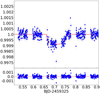 |
Fig. 4 The detrended CHEOPS light curve of planet c and best fitting transit model (upper panel). Residuals are displayed in the lower panel. |
 |
Fig. 5 Ground-based follow-up light curve of TOI-1797 b on UTC 2021 January 27 from the LCOGT 1 m network in PanSTARRS Y-band. The grey filled circles show the photometry from the individual exposures. The green filled circles show the results in 10 minute bins. The fitted transit centre time is 2459241.875 BJD, and is consistent with the ephemeris extracted from the TESS and CHEOPS data in the work. |
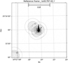 |
Fig. 6 MuSCAT 2 zoomed r-band field of view. HD 93963 A (star ID 0) was saturated on purpose to search for transit event around nearby stars. MuSCAT 2 observations ruled out star ID 7 (TIC 368435329) as the one with the 1.04 d transit signal. |
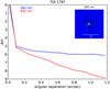 |
Fig. 7 Gemini North/Alopeke 5-sigma contrast curves and the 832 nm reconstructed speckle image. |
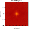 |
Fig. 8 Final combined mosaic of NIR adaptive optics image constructed from the 15-point dither pattern. The nearby companion TIC 368435331 (Gaia DR3 729899906357408640) is clearly detected ~6″ to the southwest of HD 93963 A. |
G-band magnitude, parallax, proper motion, and renormalized unit weight error (RUWE) of HD 93963 A and its companion, as retrieved from the Gaia EDR3.
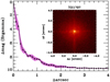 |
Fig. 9 Companion sensitivity for the Palomar adaptive optics imaging. The black points represent the 5 σ limits and are separated in steps of 1 FWHM (~0.097″); the purple represents the azimuthal dispersion (1 σ) of the contrast determinations (see text). The inset image is of the primary target showing no addtional companions to within 3″ of the target. |
5 Ground-based spectroscopy
5.1 TRES
We obtained a single reconnaissance high-resolution spectrum of HD 93963 A on 25 November 2020 using the Tillinghast Reflector Echelle Spectrograph (TRES; Fűrész 2008) mounted on the 1.5 m Tillinghast Reflector telescope at the Fred Lawrence Whipple Observatory (FLWO) atop Mount Hopkins, Arizona. TRES is a fibre-fed, optical spectrograph covering the wavelength range 390–910 nm and it has a resolving power of R = 44 000. The exposure time was 195 s, which resulted in an S/N of 35. We extracted the spectrum as described in Buch-have et al. (2010) and we derived the stellar parameters using the Spectral Parameter Classification tool (SPC; Buchhave et al. 2012, 2014). SPC cross-correlates an observed spectrum with a grid of synthetic templates to derive stellar parameters. The grid is based on Kurucz atmospheric models (Kurucz 1993). We obtained an effective temperature of Teff = 5883 ± 50 K, a surface gravity of log g* = 4.38 ± 0.10 (cgs), an iron content of [Fe/H] = 0.02 ± 0.08, and a projected rotational velocity of v sin i* = 5.3 ± 0.5 km s−1.
5.2 FIES observations
We used the FIbre-fed Échelle Spectrograph (FIES; Frandsen & Lindberg 1999; Telting et al. 2014) mounted on the 2.56 m Nordic Optical Telescope (NOT) of Roque de los Muchachos Observatory (La Palma, Spain) to acquire three high-resolution (R ≈ 67 000) spectra of HD 93963 A over a time base of nearly 15 days. The observations were carried out under good sky and seeing conditions (~1″), as part of the observing programme 62–506 (PIs: E. Knudstrup and L. M. Serrano). We set the exposure time to 1800 s, which led to an S/N ~ 70–100 per pixel at 550 nm. Following the same observing strategy adopted in Gandolfi et al. (2013, 2015), we removed cosmic ray hits by splitting each epoch observation in 3 consecutive sub-exposures of 600 s, and traced the drift of the instrument by acquiring longexposed (~140s) ThAr spectra immediately before and after each target observation. We reduced the data using standard IRAF and IDL routines and extracted the RVs via multi-order cross-correlation using the stellar spectrum with the highest S/N as a template. The three FIES RV measurements show no significant variation at a level of 10 m s−1 ruling out a short-period binary or giant planet scenario.
5.3 SOPHIE observations
Twenty-nine high-resolution spectra of HD 93963 A were obtained with the SOPHIE spectrograph (Perruchot et al. 2008; Bouchy et al. 2013) installed on the 1.93 m reflector telescope of Haute-Provence Observatory (France), between 17 November 2020 and 26 May 2021. The observations were collected as part of two programs devoted to radial velocity follow-up observations of transiting planet candidates (programme IDs: 20B.PNP.HEBR and 21A.PNP.HEBR; PI: G. Hébrard). On each of six nights, we secured 2 observations about two hours apart, in order to attempt a mass measurement of the 1.04 d planetary candidate. The observations were performed using the SOPHIE high-resolution mode (R ≈ 75 000) with simultaneous sky monitoring and an exposure time of 730 s, which led to a typical S/N = 53 per pixel at 550 nm (Table A.1). Additionally, for the characterization of the stellar host, we obtained two high S/N spectra using the SOPHIE high-efficiency mode which has a resolving power of R ≈ 40 000 (programme ID: 20B.PNP.HOYE; PI: S. Hoyer). The exposure was 1800 s, leading to S/N ≈ 128 and 156 per pixel at 550 nm (Table A.1).
The data were reduced using the SOPHIE data reduction pipeline (Bouchy et al. 2009). Radial velocities were measured by cross-correlating the extracted spectrum with a G2 binary mask and fitting a Gaussian function to the resulting cross-correlation function (CCF). We corrected the RVs for instrumental drifts by interpolating to the mid-time of exposure the drift estimated between two Fabry–Perot calibrations performed less than 2 h before and after each exposure. The SOPHIE spectrograph also presents long-term variations of the zero-point (Courcol et al. 2015). To correct for this effect, we monitored RV standard stars every night, making a master time series and subtracting them from our RVs (more details may be found in Courcol et al. 2015; Hobson et al. 2018). Finally, the data were also corrected for Moon light contamination and charge transfer inefficiency. Two measurements were not taken into account in the analysis presented in Sect. 9 due to their low S/N (<30). One measurement was obtained under bad weather conditions, whereas the other has a short exposure time, owing to a technical failure during the integration. The SOPHIE RV measurements of HD 93963 A are listed in Table A.1, along with the full width at half maximum (FWHM) and bisector inverse slope (BIS) of the CCF, and the Ca ii H & K chromospheric activity indicator log  , as extracted using the SOPHIE data reduction pipeline (Bouchy et al. 2009).
6 Stellar properties
6.1 Spectroscopic parameters
We performed the spectral analysis of HD 93963 A using the combined SOPHIE spectra, as obtained from the co-addition of the two high-efficiency mode spectra (last two lines in Table A.1). The co-added spectrum has a S/N ≈ 200 per pixel at 550nm. We derived the stellar atmospheric parameters, namely, the effective temperature Teff, surface gravity log g*, microturbulence velocity vmic, and iron abundance [Fe/H], using the ARES+MOOG codes, following the methodology described in Santos et al. (2013) and Sousa (2014). Briefly, we first computed the equivalent widths of the iron lines with the code ARES9 (Sousa et al. 2007, 2015). We then applied a minimization process to find ionization and excitation equilibrium, and to converge to the best set of spectroscopic parameters. This process makes use of a grid of Kurucz’s model atmospheres (Kurucz 1993) and the radiative transfer code MOOG (Sneden 1973). We obtained Teff = 5987 ± 64 K, log g* = 4.49 ± 0.11 (cgs), [Fe/H] = 0.10 ± 0.04 (in agreement with the TRES results presented in Sect. 5.1), and vmic = 1.15 ± 0.03 m s−1. Using the same tools, we also determined the abundance of Mg ([Mg/H] =0.08 ± 0.06) and Si ([Si/H] = 0.08 ± 0.04), closely following Adibekyan et al. (2012, 2015).
As a sanity check, we independently analysed the co-added FIES spectrum using the Specmatch-emp package (Yee et al. 2017), which compares the observed spectrum with a library of over 400 template spectra of stars of all types with well determined physical parameters. After formatting our co-added FIES spectrum to a compatible format (Hirano et al. 2018), a χ2 minimization procedure provides an estimate of the following parameters: Teff = 5875 ± 110 K, [Fe/H] = 0.10 ± 0.09, and R* = 1.10 ± 0.18 R⊕. These results are compatible within 1 σ with the parameters retrieved with ARES/MOOG. We finally utilized the package Spectroscopy Made Easy (SME, Valenti & Piskunov 1996; Piskunov & Valenti 2017) to determine the projected rotational velocity of the star v* sin i*. Based on Teff, log g* and [Fe/H] as derived with Specmatch-emp, vmic as determined with ARES/MOOG, and vmac = 4.1 ± 0.4 km s−1 from the Doyle et al. (2014)’s empirical equation, we found v* sin i* = 5.9 ± 0.8 km s−1, in very good agreement with the TRES results (see Sect. 5.1).
Using the Pecaut & Mamajek (2013)’s calibration for main sequence stars10, we found that the effective temperature implies that HD 93963 A is a G0 dwarf star. The complete set of spectroscopic parameters adopted in the current work are listed in Table 1.
6.2 Radius
To determine the stellar radius of HD 93963 A we used a modified version of the infrared flux method (IRFM; Blackwell & Shallis 1977) in a Markov chain Monte Carlo (MCMC) approach (Schanche et al. 2020). Within the IRFM MCMC, we first constructed synthetic spectral energy distributions (SEDs) from ATLAS stellar atmospheric models (Castelli & Kurucz 2003), using the photospheric parameters and their uncertainties derived with ARES+MOOG. We derived the stellar angular diameter by fitting the observed fluxes with synthetic photometry computed by convolving the ATLAS SEDs with the broadband response functions of each bandpass. The angular radius was then converted to stellar radius using the offset-corrected Gaia EDR3 parallax (Gaia Collaboration 2021; Lindegren et al. 2021). In this study, we retrieved the broadband fluxes and their uncertainties for HD 93963 A from the most recent data releases for the following bandpasses: Gaia G, GBP, and GRP, 2MASS J, H, and Ks, and WISE W1 and W2 (Gaia Collaboration 2021; Wright et al. 2010; Skrutskie et al. 2006). We found that HD 93963 A has a radius of R* = 1.043 ± 0.009 R⊙.
6.3 Rotation period
The TESS light curve of HD 93963 A shows quasi-periodic photometric variability with a peak-to-peak amplitude of ~0.2% (Fig. 1). Given the G0 V spectral type of the star, this is likely induced by the presence of active regions (spots and plages) carried around by stellar rotation.
The Lomb–Scargle periodogram (Lomb 1976; Scargle 1982) of the TESS time series displays its most significant peak at 0.159 d−1, which corresponds to a period of ~6.3 d (Fig. 10, upper panel). We computed its false alarm probability (FAP) following the bootstrap method described in Murdoch et al. (1993) and Hatzes (2019), and found it to be well below FAP < 10−6. The auto-correlation function (ACF; McQuillan et al. 2013) of the TESS light curve displays its first two correlation peaks at ~6.4 d and ~2 × 6.4 = 12.8 d (Fig. 10, lower panel). A visual inspection of the TESS light curve (Fig. 1, first panel) hints that the flux pattern repeats every ~12.8 d, suggesting that the stellar rotation period is Prot ≈ 12.8 d. We attribute the peak at 6.4d to the presence of active regions at opposite longitudes on the stellar photosphere. From the peak of the ACF and its half full width at half maximum we estimated a rotation period of Prot = 12.8 ± 1.8 d. Assuming that the star is seen equator on, the projected rotation velocity (v sin i* = 5.9±0.8 km s−1) and the stellar radius (R* = 1.043 ± 0.009 R⊙) translate into a rotation period of  d, which agrees with our finding within11 1.7 σ.
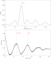 |
Fig. 10 Study of the HD 93963A rotational period using TESS data. Upper panel: Lomb–Scargle periodogram of HD 93963 A light curves. The red dashed line marks the first harmonic of the rotation frequency of the star. Lower panel: autocorrelation function of the TESS light curve. The red dashed lines mark the rotation period of the star and its first harmonic. |
6.4 Mass and age
By adopting Teff, [Fe/H], and R* as input parameters, we then determined the isochronal stellar age t* and mass M* following two different methods. The first method uses the isochrone placement technique implemented by Bonfanti et al. (2015, 2016), taking further benefit of the stellar rotation period determined from the TESS photometry Prot = 12.8 ± 1.8 d (Sect. 6.3). The knowledge of the rotation period of the star improves the convergence of the fitting procedure since it gives an additional constraint via the gyrochronological relation from Barnes (2010), as thoroughly discussed in Bonfanti et al. (2016). The isochrone placement interpolates the input parameters within pre-computed grids of stellar isochrones and tracks obtained from the PAdova & TRieste Stellar Evolutionary Code (PARSEC v1.2S, Marigo et al. 2017) to infer the stellar age and mass. The second method uses the Code Liègeois d’Évolution Stellaire (CLES, Scuflaire et al. 2008) to directly compute the evolutionary track that fits the input parameters and derive age and mass following the Levenberg-Marquardt minimization scheme (Salmon et al. 2021). After checking the consistency of the two results through a χ2-based criterion (see Bonfanti et al. 2021a, for further details), we finally combined our age and mass estimates by summing the respective probability density distributions and obtained the following median values (1 σ confidence level):  Gyr and
  M⊙.
M⊙.
As a sanity check, we further employed the python module12 stardate (Angus et al. 2019). The code combines the isochrone fitting within the MESA Isochrones & Stellar Tracks (MIST, Dotter 2016; Choi et al. 2016) with the gyrochronological relation empirically calibrated by Angus et al. (2019) in order to infer the ages of F, G, K, and M type stars. The approach is the same as in the isochrone placement of Bonfanti et al. (2016), but the theoretical models and the gyrochronological relation are different. Here we used as input the spectroscopic parameters and the photometric band values of HD 93963 A listed in Table 1. For the parallax we adopted the value in Table 3, while for the stellar rotation we injected the period of Prot = 12.8 ± 1.8 d we estimated in Sect. 6.3. We then ran an MCMC simulation, with 100 000 iterations and discarding the first 10 000 as burn in, to create the posterior distributions from which we infer the best-fit parameters. We obtained  Gyr, which is consistent with the result obtained by combining PARSEC and CLES outcomes and suggests that the star is younger than the Sun.
While we have no reason to prefer one method over the other, we adopted the results obtained with the PARSEC and CLES stellar models. Results are listed also in Table 1.
6.5 Interstellar extinction
We determined the interstellar extinction Av along the line of sight to the star following the procedure described in Gandolfi et al. (2008). Briefly, we fitted the spectral energy distribution of HD 93963 A using the synthetic magnitudes obtained by convolving the low-resolution BT-NextGen model spectrum (Allard et al. 2012) having the same spectroscopic parameters as the star, with the transmission functions of the magnitudes listed in Table 1. Using the Cardelli et al. (1989) extinction law and assuming a total-to-selective extinction ratio of Rv = Av/E(B – V) = 3.1, we found that Av = 0.10 ± 0.05, as expected given the relatively short distance to the star (~82.5 pc).
6.6 Position in galaxy
We used the systemic radial velocity reported in Table A.1 and the proper motion and parallax in Table 3 to determine the local standard of rest (LSR) U, V, and W space velocities of HD 93963 A following the methodologies in Johnson & Soderblom (1987). We did not subtract the Solar motion and computed the UVW values in the right-handed system. We obtained: U = −33.03 ± 0.04 km s−1, V = −21.42 ± 0.03 km s−1, W = −5.06 ± 0.03 km s−1. Adopting the formalism presented in Reddy et al. (2006), we used these estimates to compute the probability that HD 93963 A belongs to the galactic thin disk, thick disk, or halo stellar population. Briefly, we adopted an MC approach with 100 000 samples using the velocity dispersion standards described in Chen et al. (2021), Reddy et al. (2006), Bensby et al. (2003, 2014), and estimated the probability of the star belonging to a certain kinematic galactic family as a weighted average. We obtained that HD 93963 A has a 98.7% probability of belonging to the thin disk, while it is highly unlikely that it is part of the thick disk (1.3%) or of the halo (~0%). We additionally used the Gaia EDR3 position, proper motion, parallax, and the stellar radial velocity to compute the galactic orbit with the package galpy (integrating over 5 Gyr, Bovy 2015), from which we retrieved a galactic eccentricity of 0.09 and a high galactic Z-component of the specific relative angular momentum of ~ 1686 kpc km s−1. These results, together with our derived [Fe/H], well support the kinematic membership of the star to the galactic thin disk.
7 Joint analysis of the TESS and CHEOPS transit light curves
We performed a joint analysis of the detrended TESS and CHEOPS light curves (Sects. 2.2 and 3.2). We excluded the LCOGT data due to their poor quality when compared to the space-based TESS and CHEOPS photometry. For the joint fit, we used the software suite pyaneti (Barragán et al. 2019, 2022), which couples a Bayesian framework with an MCMC sampling to produce posterior distributions of the fitted parameters. pyaneti uses the quadratic limb-darkening transit model of Mandel & Agol (2002) following the q1 and q2 parametrization proposed by Kipping (2013). We set Gaussian priors on q1 and q2 using the limb darkening coefficients derived by Claret (2017, 2021) for the TESS and CHEOPS passbands, respectively. We imposed a conservative standard deviation of 0.1 on both the linear and quadratic terms. We sampled for the mean stellar density ρ* and recovered the scaled semi-major axis for each planet (a/R*) using Kepler’s third law (Winn 2010). In detail, we imposed a Gaussian prior on ρ* using the stellar mass and radius derived in Sect. 6. We adopted wide uninformative uniform priors for the remaining transit parameters (see Table 4), with the exception of the eccentricity and the argument of periastron, which were fixed to zero and 90°, respectively.
We explored the parameter space with 500 chains and checked for convergence using the Gelman-Rubin statistics (Gelman & Rubin 1992). Once the chains converged, we used the last 500 iterations and saved the chain states every 10 iterations, generating a posterior distribution of 250 000 points for each fitted parameter. The inferred transit parameters and their uncertainties are defined as the median and the 68% region of the credible interval of the corresponding posterior distributions (Table 5). The transit depths of  ppm and
  ppm of the 1.04 d and 3.65 d signal imply planetary radii of R⊕ = 1.35 ± 0.042 R⊕ (3% precision) and Rc = 3.228 ± 0.059 R⊕ (1.7% precision), respectively.
We checked whether the TESS and CHEOPS light curves provide consistent transit depths repeating the procedure described above, but independently modelling the transit depths within the two data-sets. Results of this sanity check are reported in Table 6. For the 3.65 d candidate TESS gives a transit depth of Dc = 812.51 ± 33.01 ppm, while the one measured by CHEOPS is 798.5 ± 32.3 ppm. For the 1.04d candidate we found that TESS gives a transit depth of Db = 131.5 ± 16.2 ppm, while CHEOPS provides  ppm. For both signals, the transit depths measured with the two instruments are consistent within 1 σ (please refer to Fig. 11 for the phase-folded transits). The CHEOPS bandpass is a broad optical bandpass very similar to that of the Gaia Gmag, providing coverage at wavelengths bluer than the red-optical TESS one. Given the different passbands, this provides evidence that the transits are achromatic, unrelated to instrumental effects.
We also tested whether the stellar density would significantly change with respect to the spectroscopic value when adopting uniform priors between 0 and 1 on the limb darkening coefficients and between 0 and 6 g cm−3 on the stellar density. This test gave a stellar density of  g cm−3 consistent with the spectroscopic density 1.379 ± 0.065 g cm−3, as well as planetary parameters compatible within 1 σ with those reported in Table 5. This implies that the stellar density is also well constrained by the transit light curves.
Priors used in the joint analysis of the TESS and CHEOPS transit light curves.
8 Validation of the two transiting planets
HD 93963 A hosts two non-grazing transiting planet candidates with periods of 3.65 d (TOI) and 1.04 d (non-TOI). The validation of the system requires ruling out the following possible false positive scenarios (see, e.g. Daylan et al. 2021; Wilson et al. 2022). The first possibility is that the transit-like events (hereafter transits in this section) might be the result of instrumental effects. The second suggests that the host star is an eclipsing binary, whose eclipses are being misinterpreted as transit features. The third scenario is that the transits might be caused by planets or stars orbiting HD 93963 B whose light leaks into the photometric mask of HD 93963 A. Finally there is a risk that planets or stars might be orbiting a background or foreground star whose light leaks into the photometric mask of HD 93963 A, generating a transit like feature.
We can exclude that the transits are due to systematics because they have been detected by two instruments (TESS and CHEOPS) with the same periods and durations. Moreover, both signals are achromatic, with TESS and CHEOPS transit depths being compatible well within 1 σ (Sect. 7), as expected from bona fide transiting planets. The measured stellar density, as derived from the modelling of the transit signal, is consistent with the spectroscopic density (Sect. 7), and the impact parameters and scaled semi-major axes imply that the orbits of the two planets are co-planar ( deg and ic = 86.31 ± 0.19 deg; Table 5), providing additional evidence that the two series of transit-like dips are actually transits of HD 93963 A.
HD 93963 A system parameters.
8.1 Contaminants in the CHEOPS field of view
An analysis of the CHEOPS FoV indicates that the level of contamination is low. Figure 12 shows the DRP simulated image of the FoV of HD 93963 A, with the red circles marking the potential sources of contamination. Given the high galactic latitude of the star (~63°), the number of contaminants is relatively small. Within the CHEOPS FoV there are 6 known Gaia sources brighter than Gaia G-band magnitude 19.5 (Table 3), with only 2 contaminants being inside the photometric aperture. Four out of the 6 contaminants are too faint (G > 17.5) and too separated from HD 93963 A to be the source of the transit signals (see below). The closest contaminant, marked as 1 in Fig. 12, is the companion HD 93963 B (see Sect. 4.4). In the following section, we show that the transit signals cannot happen on the companion HD 93963 B. The star marked with 2 in Fig. 12, is DR3 729899902062379776, a G =17.5 star located 16.8″ away from HD 93963 A. This is the only contaminant potentially capable of generating a false positive detection.
A contaminant can affect the light curve in two ways: firstly, flux from the contaminant dilutes any transit signal. Secondly, if the contaminant is an eclipsing binary (EB), it can generate a false transit detection. The dilution is already strongly mitigated, because PIPE removes contributions due to contaminants by subtracting a synthetic image produced using the PSF and parameters from the EDR3 catatalogue for the contaminant stars. This correction does not account for variability, so an EB may still induce a transit signal. The contribution of a detectable contaminant star (within 0.5″) to the PSF photometry of the target is different from the case of aperture photometry, depending on the target-contaminant separation. We can therefore do an a priori test of false positive detections for the two transits, by comparing the variability in the photometry extracted with the two methods; if the transit signal comes from the target, both methods should give consistent transit depths.
To quantify the effects of contamination on PSF and aperture photometry, we used an empirical CHEOPS PSF and computed the effects of contamination for all position angles in steps of 5 degrees. We included the angular dependence because the CHEOPS PSF is strongly asymmetric, so the contamination depends on the orientation of the PSF with respect to the contaminant. In Fig. 13, we plot the contamination fraction, which is the fraction of flux that affects the flux estimate, as a function of separation for the two photometric extraction methods and the full range of position angles. In the DRP, the assumed aperture has the default radius 25 pixels. Since the PSF drops steeply at larger radii, the dependence on its defined radius is insignificant as long as it is greater than the contaminant separation.
From the plot, we see that the contamination fraction for the two extraction methods have different dependencies on separation, but that the contamination in PSF extraction is typically a few times lower than in aperture extraction. Among the sources listed in Table 3, we confirm that the strongest contaminant is DR3 729899902062379776. At this separation, the contamination in the extracted PIPE photometry should be about 40% weaker than in the DRP photometry. A comparison of the extracted photometry from PIPE and the DRP shows about a 3% difference for both planets, consistent within the estimated measurement uncertainty of 7% and 4% for the 1.04 d and 3.65 d signals, respectively. This confirms that the transits are unlikely to be due to the contaminating star. For the 3.65 d signal, this can also be inferred from the fact that the observed transit depth of 805 ppm is stronger than the signal even a 100% occulting EB would induce, which would be 690 ppm in an R25 aperture and 480 ppm for the PSF extraction.
An additional confirmation that the 1.04 d candidate is not a false positive has been provided by the photometric in-transit observations carried out with MuSCAT 2 (Sect. 4.2). Although the transit is too shallow to be detected from the ground, the analysis of the light curve of the contaminant star DR3 729899902062379776 rules out a false positive detection due to a contaminating eclipsing binary scenario. Finally, the LCOGT observations showed that the transit of the 3.65 d period planet happens on HD 93963 A, therefore excluding the signal is a false positive caused by NEBs.
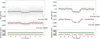 |
Fig. 11 Phase-folded light curve of planets HD 93963 Ab (left panel), and c (right panel). Upper panels: photometric measurements are shown with light grey circles, along with the 10-minute binned data (green circles for TESS, and red for CHEOPS), and the best-fitting transit model (solid black line). On the right-hand side of the plot, we also show the size of TESS and CHEOPS error-bars, respectively in green and red. Lower panels: residuals, colour-coded as above. |
Scaled planetary radii, estimated planetary radii and transit depths retrieved from the photometric joint fit that accounts for the difference in pass-bands between TESS and CHEOPS.
8.2 No transits on HD 93963 B
HD 93963 A has a gravitationally bound stellar companion at ~5.9″ south-east (Sect. 4.4). We now want to understand whether the planets transit the bright component, HD 93963 A, or the faint companion, HD 93963 B. As mentioned in Sect. 4.4, HD 93963 B is an M5V type star, that is a star with Teff.B ≈ 3060 K, M*,B ≈ 0.162 M⊙, and R*,B ≈ 0.196 R⊙ (Mamajek & Hillenbrand 2008).
If HD 93963 B were totally occulted by an inflated gas giant planet or a second M-dwarf, the diluted depth (estimated taking into account the difference of 7.9 between the G-band magnitudes of HD 93963 A and HD 93963 B) would be ~700 ppm, which is too shallow to account for the  ppm depth of the transit signal of planet c. For a 3.65-d orbit, the transit duration would be ~1.2 h for a Jupiter mass companion and shorter for a stellar companion, in disagreement with the observed duration of
  h. If HD 93963 B were totally occulted by an orbiting companion having the same size as the star, the transit would be v-shaped, while the TESS and CHEOPS transits are u-shaped.
However, the depth of the 1.04 d transit signal ( ppm) could be explained by an object transiting HD 93963 B. Based on its predicted radius of 0.196 R⊙, only a Jupiter-size object with a radius of ~0.09 R⊙ would be able to account for the detected transit depth. Yet, given the stellar radius and the scaled semi-major axis ab/RB ≈ 12, the transit duration would be ~0.9 h, which is significantly shorter than the measured duration of 1.812 ± 0.040 h. A highly-eccentric orbit could still give a longer transit duration if the transit occurred at the apocentre. On the other hand, with a period of just 1 d it is highly unlikely that the orbit is eccentric.
We conclude that the two series of transit signals do not happen on HD 93963 B given their shapes, depths, and durations. This is also corroborated by the fact that the stellar density derived from the modelling of the transit light curves is consistent with the spectroscopic density of HD 93963 A (Sect. 7).
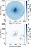 |
Fig. 12 CHEOPS images of HD 93963 FoV. Upper panel: An example of a CHEOPS subarray science image (from visit CH_PR110045_TG002001_V0200). Lower panel: DRP simulated FoV only with the background stars (therefore with the target removed), used to estimate the contamination level induced by these stars in the photometric aperture. Both panels: the orange circle represents the DEFAULT photometric aperture and the red numbered dots indicate the location of nearby stars. Due to the large difference in brightness, the background stars are barely detected in the CHEOPS science images. |
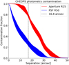 |
Fig. 13 The fraction of flux of a contaminant that affects the photometry for aperture and PSF photometry as a function of separation. The width of the lines reflect the angular dependence due to the asymmetry of the CHEOPS PSF. R25 and R50 indicate the aperture radii expressed in pixels. The dashed vertical line at 16.8″ corresponds to the separation of the most significant potential contaminant. |
8.3 Ruling out false positive scenarios
We used the Tool for Rating Interesting Candidate Exoplanets and Reliability Analysis of Transits Originating from Proximate Stars (TRICERATOPS; Giacalone et al. 2021) to further verify that the transits are not due to contaminating eclipsing binaries. TRICERATOPS is a Bayesian tool that uses the phase-folded primary transit, any pre-existing knowledge about the stellar host and contaminants, and the understanding of planet occurrence and stellar multiplicity. For each planet, the code requires the photometric phase-folded light curve (with phase equal to zero corresponding to the transit centre), the target TESS input catalogue ID and the TESS sector in which the target was observed. The code refers to the MAST database to recover the list of stars within 10 pixels (each pixel corresponds to 21″) from the target. TRICERATOPS uses these inputs to calculate the contribution of nearby stars to the observed flux, and identifies those that are bright enough to produce the observed transit. The accounted for scenarios of false positive detections are the following: an unresolved bound companion with a planet transiting the secondary star, an unresolved foreground or background star hosting a planet, a foreground or background eclipsing binary, a transit on a nearby star, and a nearby eclipsing binary (NEB). The code uses a Bayesian framework to estimate the probability associated with each scenario, by fitting transit and eclipsing binary models accounting for the input orbital period and twice the period.
We ran TRICERATOPS for both candidates. The pipeline identified a total of 23 stars within 10″ from the target star, although only 2 nearby stars were considered to be potential NEBs: the gravitationally bound stellar companion DR3 729899906357408640, and the star DR3 729899902062379776. For DR3 729899906357408640, the stellar companion, we assumed the typical mass and radius of an M5 dwarf (according to Mamajek & Hillenbrand 2008), while for DR3 729899902062379776 we had no specific assumption (specifying the spectral type does not affect the results of the analysis). We first injected phase-folded TESS data, using for Τ0 and P the values listed in Table 5. We then ran TRICERATOPS on the combination of the TESS and the CHEOPS light curves also using the values of T0 and P listed in Table 5. For both candidates we found that the signals are very likely associated with planets transiting HD 93963 A. We obtained a false positive probability of FPP ~ 0.009 and a negligible nearby false positive probability (NFPP) for the 3.65 d planet, which is therefore validated according to the TRICERATOPS criteria (FPP < 0.015 and NFPP < 0.001 for a planet to be validated). This result represents a notable improvement with respect to that obtained by Giacalone et al. (2021). Giacalone et al. (2021) ran this analysis only on the TESS data, obtaining an FPP ~ 0.3, according to which the candidate is not validated, but must be classified as “likely a planet”. In the case of the 1.04 d transit signal, the code provides an FPP ~ 0.09 and an NFPP ~ 0.006. Based on the TRICERATOPS criteria this test tells us that this object is “likely a planet” but there is a low probability of false positives due to binaries. Since planet c is already confirmed, folding in the FPP of planet c to the validation analysis of planet b would likely decrease the FPP of planet b. Furthermore, based on multiplicity statistics determined from Kepler discoveries (Lissauer et al. 2012), it is highly likely that an additional transit signal in a system with a validated planet is also planetary in nature. We therefore conclude that both planets are validated.
9 Radial velocity analysis
We performed a frequency analysis of the SOPHIE RV measurements and activity indicators to search for the Doppler reflex motions induced by HD 93963 Ab and c, and unveil the presence of possible additional RV signals arising from other orbiting planets and-or stellar activity. We estimate the expected masses of the two planets using the empirical massradius relations reported in Otegi et al. (2020). With a radius of ~1.3 R⊕, HD 93963 Ab is very likely a rocky planet with an expected planetary mass of Mb ≈ 2.4 M⊕ and an induced Doppler semi-amplitude of Kb ≈ 1.6 m s−1. With a radius of ~3.2R⊕, HD 93963 Ac might be a volatile-rich sub-Neptune (ρc < 3.3 g cm−3), or a highly dense (ρc > 3.3 g cm−3) planet rich in iron, silicates and water, with a thin gaseous envelope accounting for no more than a few per cent of the total mass, similarly to TOI-849 b (Armstrong et al. 2020). Therefore, its mass may range from Mc ≈ 10 to 50 M⊕, while the predicted radial velocity semi-amplitude ranges from Kc ≈ 5 to 23 m s−1. Given the median uncertainty of the SOPHIE RV measurements (3 ms−1; Table A.1), we should be able to detect the Doppler reflex motion induced by HD 93963 Ac.
HD 93963 A is a magnetically active solar-like star with a mean Ca ii H & K chromospheric activity indicator of log  , as derived from the SOPHIE spectra (Table A.1), and a peak-to-peak photometric variability of ~0.2%, as measured by TESS. It is well known that the presence of magnetically active regions (spots and plages) coupled to stellar rotation can induce periodic and quasi-periodic Doppler signals at the stellar rotation frequency and its harmonics. Using the code SOAP2 (Dumusque et al. 2014), we estimated the RV semi-amplitude of the activity-induced signal – the so-called activity-induced RV jitter – from the effective temperature, radius, rotation period, and photometric variability of the star. We found that the predicted semi-amplitude of the RV jitter is ~5−10 m s−1. Given the precision of the SOPHIE measurements, the stellar signal is also expected to be detected in our Doppler data.
The upper left and right panels of Fig. 14 display the generalized Lomb–Scargle periodogram (Zechmeister & Kürster 2009) of the SOPHIE RV measurements for two different frequency ranges encompassing the orbital frequencies of the two planets (fb =0.96 d−1 and fc = 0.27 d−1; vertical dashed red lines). The yellow region marks the 68.3% (1 σ) credible interval of the rotation frequency of the star, as estimated from the TESS light curve (Sect. 6.3). The horizontal dashed red line marks the false alarm probability (FAP) of 0.1%, which was estimated using the bootstrap method described in Murdoch et al. (1993) and Hatzes (2019). The periodogram of the SOPHIE RVs shows no significant peak (FAP < 0.1%)13 and weak powers at fb and fc. The null detection of the RV signal induced by planet c might be a consequence of the relatively small number of measurements (27), aliasing effects due to the sparse sampling of our SOPHIE RVs, and the presence of additional, non-accounted for Doppler signals in the data. We note that the periodogram of the SOPHIE RVs shows a peak at 0.09 d−1 (~11 d), which falls within the 68.3% credible interval of the rotation frequency of the star, and that might arise from stellar activity (vertical dashed blue line). This is corroborated by the fact that the 0.09 d−1 peak seems to have a possible counterpart in the periodogram of the FWHM of the cross-correlation function (CCF), as well as in the periodograms of log  and Ha (Fig. 14).
As HD 93963 A b and c are two bona fide, validated planets (see Sect. 8) and the Doppler reflex motion of planet c should be detectable with SOPHIE, we modelled our RV measurements with two Keplerians using the code pyaneti. We adopted Gaussian priors for the orbital periods and the times of mid-transit, as derived from the joint analysis of the TESS and CHEOPS light curves presented in Sect. 7, and uniform uninformative priors for the K-amplitudes and systemic velocity. We assumed circular orbits and added an “RV jitter term” to account for noise not included in the nominal uncertainties. While HD 93963 A b and c remain undetected (1 σ and 2.4σ level, respectively), we found a high RV jitter term of ~11.5 m s−1 (Table 7), which is ~4 times the median uncertainty of our measurements, suggesting that additional Doppler signals might be present in the data.
The panels in the second row of Fig. 14 display the periodogram of the RV residuals. Although we found no peak with FAP < 0.1%, there are two important points to note. First, there seems to be an excess of power at frequencies lower than 0.006 d−1, the spectral resolution of our SOPHIE data14, suggesting the presence of a long-term trend (blue arrow in Fig. 14). Second, the significance of the stellar signal at 0.09 d−1 has increased. We thus proceeded by modelling the activity-induced RV variation at the star’s rotation period adding a coherent sinelike curve whose period was constrained with a uniform prior centred at Prot = 12.8 d, and having a width of 4 d. For the phase and semi-amplitude of the activity signal we adopted uniform priors. While we acknowledge that this simple model might not fully reproduce the quasi-periodic variations induced by evolving active regions, it has proven to be effective in accounting for the stellar signal of active and moderately active stars (see, e.g. Hatzes et al. 2010; Barragàn et al. 2018; Gandolfi et al. 2017, Gandolfi et al. 2019).
The panels in the third row of Fig. 14 show the periodogram of the RV residuals following the subtraction of the signals arising from two planets and the star. With an FAP < 0.1%, we found that the excess of power at low frequencies has become significant (blue arrow in Fig. 14). We therefore added a linear trend to the last RV model, which includes two Keplerians plus one sine curve, and refitted the SOPHIE data with pyaneti. Based on the Bayesian information criterion (BIC) and the jitter term, we found that the model with the linear trend is preferred over the other two previous models (Table 7).
Figure 15 shows the SOPHIE RV time series and the phase-folded RV curves of HD 93963 A b and c, along with the best fitting models. The inferred parameters are given in Table 8. With an RV semi-amplitude variation of Kc = 7.4± 1.6m s−1, HD 93963 A c is significantly detected in the SOPHIE measurements (4.6 σ), while HD 93963 A b is not significantly detected in our data (Kb = 4.6± 1.9 m s−1; 2.6 σ). The stellar RV signal has an amplitude of 10.4 ± 2.1 m s−1, as predicted by SOAP2. We also found evidence of the presence of a linear trend in the data with an acceleration of 0.13 ± 0.02ms−1 d−1. Although the periodogram of the FWHM shows an excess of power at low frequencies, the corresponding peak is not significant to claim that this signal arises from stellar activity. The source and periodicity are hard to pinpoint given the ~180-d baseline of our radial-velocity campaign with SOPHIE. Longer baseline RV campaigns should be performed in order to unveil the true nature of this long period signal.
Bayesian information criterion (BIC) and jitter term of the three different models considered for our RV-only analysis.
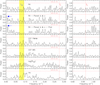 |
Fig. 14 Generalized Lomb-Scargle periodograms of the SOPHIE RV measurements and activity indicators. The right and left columns cover two frequency ranges encompassing the orbital frequencies of HD 93963 A b and c (fb = 0.96 d−1 and fc = 0.27 d−1; vertical dashed red lines) and the 68.3% credible interval of the rotation frequency of the star (yellow area), as estimated from the TESS light curve. The vertical dashed blue line marks the rotation frequency of the star (frot = 0.09−1, which implies Prot ~ 11.1 d), as derived from the SOPHIE data. From top to bottom: RV data; RV residuals after subtracting the signals of the two transiting planets; RV residuals after subtracting the signals of the star and of the two transiting planets; FWHM and BIS of the CCF; log |

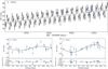 |
Fig. 15 Upper panel: SOPHIE RV time series and best fitting model. Lower panels: phase-folded RV curve of HD 93963 A b (left), HD 93963 A c (right) and best-fitting Keplerian model. The vertical grey lines mark the error bars including the RV jitter. |
Best fitting parameters and planetary masses as derived from the analysis of the SOPHIE RV measurements.
10 Discussion and conclusions
HD 93963 A is a northern (δ ≈ +25°), young (~1.4 Gyr), visual binary at 82.5 pc from the Sun consisting of a bright (G = 9.0) G0V star and a ΔG = 7.8 magnitudes fainter M-type dwarf. The two stars have an angular separation of ~5.9″, which corresponds to a sky-projected separation of ~484 AU.
The brightest component has a rotation period of Prot = 12.8 ± 1.8 d (as estimated from the TESS light curve), a mass of M* = 1.109 ± 0.043 M⊙, a radius of R* = 1.043 ± 0.009 R⊙, an effective temperature of Teff = 5987 ± 64 K, and an iron content of [Fe/H] =0.10 ± 0.04. HD 93963 B is an M5V star, with an estimated mass of ~0.16 M⊙ and radius of ~0.20 R⊙. If we assume that the orbit of the smaller companion is seen face on and that the eccentricity is zero, we can use Kepler’s third law to estimate that the binary has an orbital period of about 8875 yr.
HD 93963 A hosts two transiting small planets, namely, HD 93963 Ab and HD 93963 Ac. The inner planet, HD 93963 Ab, is a hot super-Earth with an orbital period of ~1.04 d, aradius of Rb =1.35 ± 0.042 R⊕, a predicted mass of Mb ≈ 2.4 M⊕ (according to the mass-radius empirical relation from Otegi et al. 2020), and an equilibrium temperature of Teq,b = 2042 ± 27 K (assuming zero albedo). Based on its orbital period and radius, HD 93963 Ab can be classified as a small ultra-short period (USP) planet, the first USP planet discovered and validated by TESS and CHEOPS. The outer planet, HD 93963 Ac, is a sub-Neptune with an orbital period of ~3.65 d, a radius of Rc = 3.228 ± 0.059 R⊕, and an RV-determined mass of Mc = 19.2 ± 4.1 M⊕, implying a mean density of ρc = 3.1 ± 0.7 g cm−3. Given the vicinity to its host star, HD 93963 A c is also hot, with an equilibrium temperature of Teq,c = 1344 ± 18 K. With inclinations of  deg and ic = 86.31 ± 0.19 deg, the orbits of the two planets might be coplanar.
In Fig. 16, we show the position of the two planets in the planetary radius-insolation scatter plot. HD 93963 A b and c fall on opposite sides of the so-called radius valley, a gap identified in the bi-modal distribution of small exoplanet radii (Fulton et al. 2017; Van Eylen et al. 2018). This gap is predicted by photo-evaporation models, which suggest that the loss of H/He atmospheres in close-in planets is a consequence of the strong stellar irradiation (Lopez & Fortney 2014). The two planets might have experienced drastically different evolution processes. Due to its semi-major axis ab = AU, which implies a strong irradiation from the star (~2900 F⊕, see Table 5), the atmosphere of HD 93963 A b probably underwent photo-evaporation (Owen et al. 2020) and now the planet has no gaseous content. For HD 93963 A c, the position in the radius-insolation plot is insufficient to conclude on the possible presence of an atmosphere. We therefore refer to the mass-radius diagram in Fig. 17, where the planet is marked as a red circle. We notice that HD 93963 Ac is located in a low populated area of the diagram. The only close-by planets are TOI-132b (Mp = 22.8 M⊕, RP = 3.4 R⊕, PP =2.1 d; Díaz et al. 2020), K2-25b (Mp = 24.5 M⊕ RP = 3.4 R⊕, PP = 3.5 d; Stefansson et al. 2020), NGTS-4b (Mp =20.6 M⊕, PP = 3.2 R⊕, Pp = 1.3 d; West et al. 2019) and TOI-824b (Mp = 18.5 M⊕, RP = 2.9 R⊕, Pp = 1.4 d; Burt et al. 2020), for which an atmosphere rich in volatiles has been predicted. We can therefore suppose that HD 93963 Ac is surrounded by a primary (therefore H/He-dominated) atmosphere, an hypothesis corroborated by the mean density of the planet (ρc = 3.1 ± 0.7g cm−3) being significantly lower than that of Earth and by its position in the mass-radius diagram above the 100% H2O composition.
To confirm our predictions on the atmospheric content of both planets and to derive an independent constraint on the mass of HD 93963 A b, we employed the tool Planetary Atmospheres and Stellar RoTation RAtes (PASTA; Bonfanti et al. 2021b). Starting from the measured system parameters, PASTA returns posterior probability distributions for the initial atmospheric mass fraction of each planet and for the evolution of the stellar rotation rate. To this end, PASTA uses the connection existing between the rotation rate and high-energy (mainly X-ray and EUV) emission of late-type stars and, through this, traces the impact of the stellar high-energy emission on planetary atmospheric escape throughout the system lifetime.
We found that HD 93963 A c can only host an atmosphere if at young ages the stellar rotation period was shorter than the average value measured for stars in young open clusters (Johnstone et al. 2015). This is shown in the top panel of Fig. 18, which presents the posterior probability distribution of the stellar rotation rate at an age of 150 Myr derived by PASTA. Although this posterior does not have a narrow peak, it clearly favours rotation evolutionary tracks slower than those measured for stars member of young open clusters that we use as a comparison: if at a young age the host star was rotating fast (emitting a larger amount of X-ray and EUV radiation), HD 93963 A c would have completely lost its atmosphere, in contradiction to its measured average density.
Using the constraint on the evolution of the stellar rotation rate, PASTA simultaneously provides a constraint on the mass of HD 93963 A b. We find that the posterior probability distribution for the mass of HD 93963 Ab is centred around 2.4 M⊕ (left-middle panel of Fig. 18). Combined with the measured planetary radius, this value leads to an Earth-like density, and thus it confirms our prediction that HD 93963 A b has completely lost its primary atmosphere through escape.
Finally, PASTA enables one to constrain the initial atmospheric mass fraction), which is the mass of a planetary atmosphere (in planetary masses) at the time of the dispersal of the protoplanetary nebula. The posterior probability distributions of for both planets are shown in the bottom panels of Fig. 18. A HD 93963 Ab has completely lost its primary atmosphere at some point in the past, PASTA is unable to constrain the initial atmospheric mass fraction. For HD 93963 A c, instead, PASTA derives an initial atmospheric mass fraction peaking around 0.15 planetary masses, which is about 50 times higher than the estimated current atmospheric content (about 0.004 planetary masses; black line in the bottom-right panel of Fig. 18).
Using the stellar photospheric abundances of Mg, Si, and Fe and the stoichiometric model presented in Santos et al. (2015, 2017), we estimated the iron mass fraction (firon) of the planet building blocks assuming that the host star composition reflects the composition of the protoplanetary disk. For firon we obtained a value of 34.4 ± 2.8%, which is larger than that of our Earth ~32% (McDonough 2003) and of the planet building blocks of our Solar System (33.2 ± 1.7%) estimated with the aforementioned stoichiometric model. Recently, Adibekyan et al. (2021a) showed that there is a statistically significant correlation between firon and the density of terrestrial planets normalized to the density of a planet with an Earth-like composition (Dorn et al. 2017). The normalization accounts for the dependence of planet’s density on the planet mass for the same composition. This finding was further confirmed by Adibekyan et al. (2021b) based on a slightly larger sample. Using the aforementioned relation between the normalized density (ρ/ρEaith–like) and firon we estimated the ρ/ρEaith–like of HD 93963 b to be 1.01 ± 0.34. This value combined with the planet radius allowed us to estimate the mass of  M⊕, which is slightly larger but within the uncertainties consistent with the one computed with PASTA and the mass predicted using the mass-radius relation of Otegi et al. (2020). We could not constrain the iron composition of the two planets, although in Adibekyan et al. (2021a) the authors found that the iron mass fraction of potentially rocky planets is usually larger than that expected from the host star composition.
HD 93963 Ab belongs to the family of small (Rp = 1−2 R⊕) USP planets, high-density rocky objects (> 4.5 g cm−3) with occurrence rates ranging from ~1.1% for M-type dwarfs to ~0.15% for F-type dwarfs (Winn et al. 2018). Small USP planets are thought to be stripped cores of former warm Neptunes and mini-Neptunes with radii between 2 and 4 R⊕, which underwent photo-evaporation processes (Lundkvist et al. 2016; Sanchis-Ojeda et al. 2014). As we demonstrated with our analysis, this is likely the case for HD 93963 A b, which is expected to have completely lost its primary atmosphere. In addition, similarly to most USP small planets, HD 93963 A b belongs to a packed multiplanet system, which includes a second planet on a 3.65 d orbit, and our SOPHIE RV measurements show a linear trend (Sect. 9), suggesting the possible presence of an additional, long-period planet orbiting the star.
Ultra-short period planets likely formed further out in the system, before migrating to the close-in orbit where it is now. Petrovich et al. (2019) proposed a secular migration scenario in which the planets of the systems are initially on highly eccentric and highly mutually inclined (>30°) orbits. As migration begins, the eccentricities are damped out on timescales from kyr to Myr (although the current value could still be well different from zero), due to tidal dissipation within the planets, while the orbital inclinations are damped out on timescales of Gyrs by the dissipation inside the host star (Winn et al. 2018). As a result the planets of the system reached stabilization on highly mutually inclined and-or highly eccentric orbits. This model could work for HD 93963 A if the planets were on highly eccentric orbits (≳0.1) and it has been shown to work for many systems hosting USP planets (Dai et al. 2018; Kamiaka et al. 2019). On the other hand, HD 93963 A might be a coplanar system, and it therefore might have migrated through another secular process, as reported by Petrovich et al. (2019) in their Sect. 5.2.2. According to this migration channel, the planets were in orbits with low eccentricities and low mutual inclinations when they started migrating. The migration process happens in a non-violent way, with the eccentricities damped to zero by tidal forces and small inclination fluctuations. After a few Gyr, the planets in the system should be nearly coplanar, comprising a USP planet and a second companion with period shorter than 10 d. Only a small number of systems with USP planets have reached these final conditions: TOI-561 (Lacedelli et al. 2021), TOI-500 (Serrano et al. 2022), CoRoT-7 (Léger et al. 2009; Hatzes et al. 2010; Haywood et al. 2014; Faria et al. 2016). Unlike this small subset of systems, HD 93963 A is a young star, meaning that for this model to work the planets should have already been on coplanar or almost coplanar orbits when they started migrating. Compared to other multi-planet systems with USP planets, HD 93963 A has a relatively close spacing between the orbits of the inner two planets (comparable to CoRoT-7 and Kepler-42). This limits the possible extent of the migration of planet b, both because stability considerations set an outer limit for the orbit of planet b (it must have been far enough from HD 93963 A c at 3.65 d), and because the available angular momentum deficit in the system that could drive tidal migration would have been limited. The latter problem can be ameliorated if additional planets exist on exterior orbits.
In this context, it is also interesting to consider the possible influence of the binary companion on the system dynamics. While the system at present is extremely hierarchical, an inclined binary companion would attempt to impose Lidov-Kozai cycles on the planets (Lidov 1962; Kozai 1962). If the binary is on a circular orbit at its projected separation of 484 AU, the timescale for these to act on HD 93963 A c is (see Valtonen & Karttunen 2006, Eq. (9.48)) ~1 Gyr, comparable to the system age, and would be longer if the binary were currently at pericentre on a wider orbit. Because of the stronger coupling between the two planets, Lidov–Kozai eccentricity cycles should be suppressed, with the planets maintaining coplanarity while becoming misaligned with the stellar equator, as in the similar system of 55 Cnc (Kaib et al. 2011). The timescale for this misalignment to be generated would be considerably reduced if additional undetected planets existed in the system. A measurement of misalignment between the stellar spin and the planetary orbits, via the Rossiter–McLaughlin effect, would therefore suggest the presence of one or more planets beyond HD 93963 A c.
HD 93963 A b is the first small USP planet confirmed and validated by TESS and CHEOPS. Further observations of the HD 93963 A system have the potential to yield new discoveries. It is a compact planetary system around a bright star that is easily accessible from the northern hemisphere. For instance, it can be observed from November until June with HARPS-N, the high-precision spectrograph mounted at the Telescopio Nazionale Galileo in La Palma (Spain). An intensive RV campaign with a spectrograph capable of reaching a precision of ~1 m s−1 would improve the precision on the mass of HD 93963 A c, measure the mass of HD 93963 A b, constrain the eccentricities of both planets, detect additional planetary companions, and monitor the long-term trend in order to unveil its origin (stellar or planetary). Such observations would enable the study of the system architecture, providing the “ingredients” necessary to constrain the migration process. Since HD 93963 A is a relatively young star (~1.4 Gyr) hosting at least two small planets, we would be able to impose stronger constraints on the time scale of the migration process.
The precise RV follow up would finally allow us to add HD 93963 A to the relatively small sample of multi-planet systems hosting a small USP planet with both masses and radii measured, which currently counts 14 members (K2-141, TOI-561, Kepler-42, K2-106, K2-229, Kepler-407, 55 Cnc, LTT 3780, WASP-47, Kepler-32, Kepler-10, CoRoT -7, HD 3167 and TOI-500; see, e.g. the TEPCat catatalogue, Southworth et al. 2011, for references). Increasing this sample is fundamental to better constrain the theory of formation and migration of exotic objects such as USP planets and, more in general, of tightly packed multi-planet systems. Especially for HD 93963 A, the measurement of the planetary masses and eccentricities will allow us to perform stability analysis and understand whether the low-eccentricity migration process described in Sect. 10 could explain its current architecture.
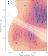 |
Fig. 16 HD 93963 A b & c (filled triangles) as a function of planetary radius and insolation, compared with the population of exoplanets. Colours represent a kernel density estimation (KDE) applied to small (Rp < 4 R⊕), transiting planets retrieved from the NASA Exoplanet Archive (Akeson et al. 2013). The dashed and dotted lines (with associated 1 σ white error bands) show estimates for the position of the evaporation valley from Martinez et al. (2019) and Van Eylen et al. (2018) respectively. |
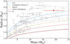 |
Fig. 17 Mass–radius diagram for small planets (RP < 4 R⊕), as retrieved from the catalogue for transiting planets TEPCat (Southworth et al. 2011). Planets whose masses and radii are known with a precision better than 22% are plotted with grey circles. The solid red circle marks the position of HD 93963 A c. Planets in the literature are marked with grey circles. Composition models from Zeng et al. (2016) are displayed with different lines and colours. |
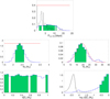 |
Fig. 18 Results of the PASTA modelling. Upper panel: posterior-distribution of the stellar rotation rate at an age of 150 Myr. The black line represents the distribution measured from a sample of open cluster stars of comparable mass and age (Johnstone et al. 2015). Middle and lower panels: posterior-distributions of planetary mass (middle) and initial atmospheric mass fraction (bottom) for HD 93963 Ab and c. The red lines represent the imposed priors (uniform or Gaussian), while in the bottom-right panel the black line shows the current atmospheric mass fraction estimated by PASTA on the basis of the measured planetary mass and radius and estimated equilibrium temperature. We note that the x axis of the bottom-left panel is in linear scale, while that of the bottom-right panel is in logarithmic scale. |
Acknowledgements
CHEOPS is an ESA mission in partnership with Switzerland with important contributions to the payload and the ground segment from Austria, Belgium, France, Germany, Hungary, Italy, Portugal, Spain, Sweden, and the United Kingdom. The CHEOPS Consortium would like to gratefully acknowledge the support received by all the agencies, offices, universities, and industries involved. Their flexibility and willingness to explore new approaches were essential to the success of this mission. We acknowledge the use of public TESS data from pipelines at the TESS Science Office and at the TESS Science Processing Operations Center. Resources supporting this work were provided by the NASA High-End Computing (HEC) Program through the NASA Advanced Supercomputing (NAS) Division at Ames Research Center for the production of the SPOC data products. This research has made use of the NASA Exoplanet Archive, of the Exoplanet Follow-up Observation Program website, which are operated by the California Institute of Technology, under contract with the National Aeronautics and Space Administration under the Exoplanet Exploration Program. L.M.S. and D.G. gratefully acknowledges financial support from the CRT foundation under Grant No. 2018.2323 “Gaseous or rocky? Unveiling the nature of small worlds”. S.H. gratefully acknowledges CNES funding through the grant 837319. ABr was supported by the SNSA. S.G.S. acknowledge support from FCT through FCT contract nr. CEECIND/00826/2018 and POPH/FSE (EC). Some of the observations in the paper made use of the High-Resolution Imaging instrument ‘Alopeke obtained under Gemini LLP Proposal Number: GN/S-2021A-LP-105. ‘Alopeke was funded by the NASA Exoplanet Exploration Program and built at the NASA Ames Research Center by Steve B. Howell, Nic Scott, Elliott P. Horch, and Emmett Quigley. Alopeke was mounted on the Gemini North (and/or South) telescope of the international Gemini Observatory, a programme of NSF’s OIR Lab, which is managed by the Association of Universities for Research in Astronomy (AURA) under a cooperative agreement with the National Science Foundation. on behalf of the Gemini partnership: the National Science Foundation (United States), National Research Council (Canada), Agencia Nacional de Investigación y Desarrollo (Chile), Ministerio de Ciencia, Tecnologia e Innovación (Argentina), Ministério da Ciência, Tecnologia, Inovações e Comunicações (Brazil), and Korea Astronomy and Space Science Institute (Republic of Korea). A.C.C. and T.W. acknowledge support from STFC consolidated grant number ST/M001296/1. M.F. and C.M.P. gratefully acknowledge the support of the Swedish National Space Agency (DNR 65/19, 174/18). This project was supported by the CNES. unding for the Stellar Astrophysics Centre is provided by The Danish National Research Foundation (Grant agreement no.: DNRF106). This work makes use of observations from the LCOGT network. LCOGT telescope time was granted by NOIRLab through the Mid-Scale Innovations Program (MSIP). MSIP is funded by NSF. Y.A. and M.J.H. acknowledge the support of the Swiss National Fund under grant 200020_172746. We acknowledge support from the Spanish Ministry of Science and Innovation and the European Regional Development Fund through grants ESP2016-80435-C2-1-R, ESP2016-80435-C2-2-R, PGC2018-098153-B-C33, PGC2018-098153-B-C31, ESP2017-87676-C5-1-R, MDM-2017-0737 Unidad de Excelencia Maria de Maeztu-Centro de Astrobiología (INTA-CSIC), as well as the support of the Generalitat de Catalunya/CERCA programme. The MOC activities have been supported by the ESA contract no. 4000124370. S.C.C.B. acknowledges support from FCT through FCT contracts nr. IF/01312/2014/CP1215/CT0004. X.B., S.C., D.G., M.F. and J.L. acknowledge their role as ESA-appointed CHEOPS science team members. P.C. thanks the LSSTC Data Science Fellowship Program, which is funded by LSSTC, NSF Cybertraining Grant Number 1829740, the Brinson Foundation, and the Moore Foundation. Her participation in the programme has benefited this work. A.De. acknowledges support from the European Research Council (ERC) under the European Union’s Horizon 2020 research and innovation programme (project FOUR ACES, grant agreement no. 724427), and from the National Centre for Competence in Research “PlanetS” supported by the Swiss National Science Foundation (SNSF). The Belgian participation to CHEOPS has been supported by the Belgian Federal Science Policy Office (BELSPO) in the framework of the PRODEX Program, and by the University of Liège through an ARC grant for Concerted Research Actions financed by the Wallonia-Brussels Federation. L.D. is an F.R.S.-FNRS Postdoctoral Researcher. This work was supported by FCT – Fundação para a Ciência e a Tecnologia through national funds and by FEDER through COMPETE2020 – Programa Operacional Competitividade e Internacionalizacão by these grants: UID/FIS/04434/2019, UIDB/04434/2020, UIDP/04434/2020, PTDC/FIS-AST/32113/2017 & POCI-01-0145-FEDER-032113, PTDC/FIS-AST/28953/2017 & POCI-01-0145-FEDER-028953, PTDC/FIS-AST/28987/2017 & POCI-01-0145-FEDER-028987, O.D.S.D. is supported in the form of work contract (DL 57/2016/CP1364/CT0004) funded by national funds through FCT. B.-O.D. acknowledges support from the Swiss National Science Foundation (PP00P2-190080). This project has received funding from the European Research Council (ERC) under the European Union’s Horizon 2020 research and innovation programme (project FOUR ACES grant agreement No 724427). ZG was supported by the VEGA grant of the Slovak Academy of Sciences number 2/0031/22, and by the Slovak Research and Development Agency - the contract no. APVV-20-0148. M.G. is an F.R.S.-FNRS Senior Research Associate. C.X.H.’s work was funded by the Australian Government through the Australian Research Council. K.G.I. is the ESA CHEOPS Project Scientist and is responsible for the ESA CHEOPS Guest Observers Programme. She does not participate in, or contribute to, the definition of the Guaranteed Time Programme of the CHEOPS mission through which observations described in this paper have been taken, nor to any aspect of target selection for the programme. This work was granted access to the HPC resources of MesoPSL financed by the Region Ile de France and the project Equip@Meso (reference ANR-10-EQPX-29-01) of the programme Investissements d’Avenir supervised by the Agence Nationale pour la Recherche. M.L. acknowledges support of the Swiss National Science Foundation under grant number PCEFP2_194576. P.M. acknowledges support from STFC research grant number ST/M001040/1. This work is partly supported by JSPS KAKENHI Grant Number JP17H04574, JP18H05439, JST CREST Grant Number JPMJCR1761, the Astrobiology Center of National Institutes of Natural Sciences (NINS) (Grant Number AB031010). This article is based on observations made with the MuSCAT2 instrument, developed by ABC, at Telescopio Carlos Sanchez operated on the island of Tenerife by the IAC in the Spanish Observatorio del Teide. This work was also partially supported by a grant from the Simons Foundation (PI Queloz, grant number 327127). Acknowledges support from the Spanish Ministry of Science and Innovation and the European Regional Development Fund through grant PGC2018-098153-B-C33, as well as the support of the Generalitat de Catalunya/CERCA programme. Gy.M.Sz. and Z.G. acknowledges the support of the Hungarian National Research, Development and Innovation Office (NKFIH) grant K-125015, a PRODEX Institute Agreement between the ELTE Eötvös Lorand University and the European Space Agency (ESA-D/SCI-LE-2021-0025), the Lendület LP2018-7/2021 grant of the Hungarian Academy of Science and the support of the city of Szombathely. V.V.G. is an F.R.S.-FNRS Research Associate.
Appendix A SOPHIE data
In Table A.1 we report the radial velocity data of HD 93963 A obtainedwith SOPHIE instrument. Thelasttwo rows correspond to the observations acquired using the high-efficiency mode of the instrument.
Radial velocity measurements of HD 93963 A obtained with the SOPHIE spectrograph.
References
- Adibekyan, V. Z., Sousa, S. G., Santos, N. C., et al. 2012, A&A, 545, A32 [NASA ADS] [CrossRef] [EDP Sciences] [Google Scholar]
- Adibekyan, V., Figueira, P., Santos, N. C., et al. 2015, A&A, 583, A94 [NASA ADS] [CrossRef] [EDP Sciences] [Google Scholar]
- Adibekyan, V., Dorn, C., Sousa, S. G., et al. 2021a, Science, 374, 330 [NASA ADS] [CrossRef] [Google Scholar]
- Adibekyan, V., Santos, N. C., Dorn, C., et al. 2021b, Commun. Byurakan Astrophys. Observ., 68, 447 [NASA ADS] [CrossRef] [Google Scholar]
- Akeson, R., Chen, X., Ciardi, D., et al. 2013, PASP, 125, 989 [CrossRef] [Google Scholar]
- Allard, F., Homeier, D., & Freytag, B. 2012, Philos. Trans. Roy. Soc. Lond. A, 370, 2765 [NASA ADS] [Google Scholar]
- Angus, R., Morton, T. D., Foreman-Mackey, D., et al. 2019, AJ, 158, 173 [Google Scholar]
- Armstrong, D. J., Lopez, T.A., Adibekyan, V., et al. 2020, Nature, 583, 39 [NASA ADS] [CrossRef] [Google Scholar]
- Baglin, A., Auvergne, M., Boisnard, L., et al. 2006, in 36th COSPAR Scientific Assembly, 36, 3749 [NASA ADS] [Google Scholar]
- Barnes, S. A. 2010, ApJ, 722, 222 [Google Scholar]
- Barragàn, O., Gandolfi, D., Dai, F., et al. 2018, A&A, 612, A95 [CrossRef] [EDP Sciences] [Google Scholar]
- Barragán, O., Gandolfi, D., & Antoniciello, G. 2019, MNRAS, 482, 1017 [Google Scholar]
- Barragán, O., Aigrain, S., Rajpaul, V. M., & Zicher, N. 2022, MNRAS, 509, 866 [Google Scholar]
- Bensby, T., Feltzing, S., & Lundström, I. 2003, A&A, 410, 527 [CrossRef] [EDP Sciences] [Google Scholar]
- Bensby, T., Feltzing, S., & Oey, M. S. 2014, A&A, 562, A71 [NASA ADS] [CrossRef] [EDP Sciences] [Google Scholar]
- Benz, W., Broeg, C., Fortier, A., et al. 2021, Exp. Astron., 51, 109 [Google Scholar]
- Blackwell, D. E., & Shallis, M. J. 1977, MNRAS, 180, 177 [NASA ADS] [CrossRef] [Google Scholar]
- Bonfanti, A., Ortolani, S., Piotto, G., & Nascimbeni, V. 2015, A&A, 575, A18 [NASA ADS] [CrossRef] [EDP Sciences] [Google Scholar]
- Bonfanti, A., Ortolani, S., & Nascimbeni, V. 2016, A&A, 585, A5 [NASA ADS] [CrossRef] [EDP Sciences] [Google Scholar]
- Bonfanti, A., Delrez, L., Hooton, M. J., et al. 2021a, A&A, 646, A157 [EDP Sciences] [Google Scholar]
- Bonfanti, A., Fossati, L., Kubyshkina, D., & Cubillos, P. E. 2021b, A&A, 656, A157 [NASA ADS] [CrossRef] [EDP Sciences] [Google Scholar]
- Borsato, L., Piotto, G., Gandolfi, D., et al. 2021, MNRAS, 506, 3810 [NASA ADS] [CrossRef] [Google Scholar]
- Borucki, W. J., Koch, D., Basri, G., et al. 2010, Science, 327, 977 [Google Scholar]
- Bouchy, F., Hébrard, G., Udry, S., et al. 2009, A&A, 505, 853 [NASA ADS] [CrossRef] [EDP Sciences] [Google Scholar]
- Bouchy, F., Díaz, R. F., Hébrard, G., et al. 2013, A&A, 549, A49 [NASA ADS] [CrossRef] [EDP Sciences] [Google Scholar]
- Bovy, J. 2015, ApJS, 216, 29 [NASA ADS] [CrossRef] [Google Scholar]
- Brown, T. M., Baliber, N., Bianco, F. B., et al. 2013, PASP, 125, 1031 [Google Scholar]
- Buchhave, L. A., Bakos, G. Á., Hartman, J. D., et al. 2010, ApJ, 720, 1118 [NASA ADS] [CrossRef] [Google Scholar]
- Buchhave, L. A., Latham, D., Johansen, A., et al. 2012, Nature, 486, 375 [NASA ADS] [CrossRef] [Google Scholar]
- Buchhave, L. A., Bizzarro, M., Latham, D. W., et al. 2014, Nature, 509, 593 [Google Scholar]
- Burt, J. A., Nielsen, L. D., Quinn, S. N., et al. 2020, AJ, 160, 153 [Google Scholar]
- Cabrera, J., Csizmadia, S., Erikson, A., Rauer, H., & Kirste, S. 2012, A&A, 548, A44 [NASA ADS] [CrossRef] [EDP Sciences] [Google Scholar]
- Cardelli, J. A., Clayton, G. C., & Mathis, J. S. 1989, ApJ, 345, 245 [Google Scholar]
- Carleo, I., Gandolfi, D., Barragán, O., et al. 2020, AJ, 160, 114 [Google Scholar]
- Castelli, F., & Kurucz, R. L. 2003, in IAU Symposium, Modelling of Stellar Atmospheres, eds. N. Piskunov, W.W. Weiss, & D.F. Gray, 210, A20 [NASA ADS] [Google Scholar]
- Chen, D.-C., Yang, J.-Y., Xie, J.-W., et al. 2021, AJ, 162, 100 [NASA ADS] [CrossRef] [Google Scholar]
- Choi, J., Dotter, A., Conroy, C., et al. 2016, ApJ, 823, 102 [Google Scholar]
- Ciardi, D. R., Beichman, C. A., Horch, E. P., & Howell, S. B. 2015, ApJ, 805, 16 [NASA ADS] [CrossRef] [Google Scholar]
- Claret, A. 2017, A&A, 600, A30 [NASA ADS] [CrossRef] [EDP Sciences] [Google Scholar]
- Claret, A. 2021, RNAAS, 5, 13 [NASA ADS] [Google Scholar]
- Collins, K. A., Kielkopf, J. F., Stassun, K. G., & Hessman, F. V. 2017, AJ, 153, 77 [Google Scholar]
- Cosentino, R., Lovis, C., Pepe, F., et al. 2012, SPIE Conf. Ser., 8446, 84461V [Google Scholar]
- Courcol, B., Bouchy, F., Pepe, F., et al. 2015, A&A, 581, A38 [NASA ADS] [CrossRef] [EDP Sciences] [Google Scholar]
- Cutri, R. M., Wright, E. L., Conrow, T., et al. 2013, VizieR Online Data Catalog: II/328 [Google Scholar]
- Dai, F., Masuda, K., & Winn, J. N. 2018, ApJ, 864, L38 [NASA ADS] [CrossRef] [Google Scholar]
- Daylan, T., Pinglé, K., Wright, J., et al. 2021, AJ, 161, 85 [NASA ADS] [CrossRef] [Google Scholar]
- Dekany, R., Roberts, J., Burruss, R., et al. 2013, ApJ, 776, 130 [CrossRef] [Google Scholar]
- Delrez, L., Ehrenreich, D., Alibert, Y., et al. 2021, Nat. Astron., 5, 775 [NASA ADS] [CrossRef] [Google Scholar]
- Díaz, M. R., Jenkins, J. S., Gandolfi, D., et al. 2020, MNRAS, 493, 973 [Google Scholar]
- Dorn, C., Venturini, J., Khan, A., et al. 2017, A&A, 597, A37 [NASA ADS] [CrossRef] [EDP Sciences] [Google Scholar]
- Dotter, A. 2016, ApJS, 222, 8 [Google Scholar]
- Doyle, A. P., Davies, G. R., Smalley, B., Chaplin, W. J., & Elsworth, Y. 2014, MNRAS, 444, 3592 [Google Scholar]
- Dumusque, X., Boisse, I., & Santos, N. C. 2014, ApJ, 796, 132 [NASA ADS] [CrossRef] [Google Scholar]
- Faria, J. P., Haywood, R. D., Brewer, B. J., et al. 2016, A&A, 588, A31 [NASA ADS] [CrossRef] [EDP Sciences] [Google Scholar]
- Fűrész, G. 2008, PhD thesis, University of Szeged, Hungary [Google Scholar]
- Frandsen, S., & Lindberg, B. 1999, in Astrophysics with the NOT, eds. H. Karttunen, & V. Piirola, 71 [Google Scholar]
- Fulton, B. J., Petigura, E. A., Howard, A. W., et al. 2017, AJ, 154, 109 [Google Scholar]
- Furlan, E., Ciardi, D. R., Everett, M. E., et al. 2017, AJ, 153, 71 [NASA ADS] [CrossRef] [Google Scholar]
- Gaia Collaboration (Brown, A.G.A., et al.) 2018, A&A, 616, A1 [NASA ADS] [CrossRef] [EDP Sciences] [Google Scholar]
- Gaia Collaboration (Brown, A.G.A., et al.) 2021, A&A, 649, A1 [NASA ADS] [CrossRef] [EDP Sciences] [Google Scholar]
- Gandolfi, D., Alcalá, J. M., Leccia, S., et al. 2008, ApJ, 687, 1303 [Google Scholar]
- Gandolfi, D., Parviainen, H., Fridlund, M., et al. 2013, A&A, 557, A74 [NASA ADS] [CrossRef] [EDP Sciences] [Google Scholar]
- Gandolfi, D., Parviainen, H., Deeg, H. J., et al. 2015, A&A, 576, A11 [NASA ADS] [CrossRef] [EDP Sciences] [Google Scholar]
- Gandolfi, D., Barragán, O., Hatzes, A. P., et al. 2017, AJ, 154, 123 [NASA ADS] [CrossRef] [Google Scholar]
- Gandolfi, D., Fossati, L., Livingston, J. H., et al. 2019, ApJ, 876, L24 [Google Scholar]
- Gelman, A., & Rubin, D. B. 1992, Stat. Sci., 7, 457 [Google Scholar]
- Giacalone, S., Dressing, C. D., Jensen, E. L. N., et al. 2021, AJ, 161, 24 [Google Scholar]
- Grziwa, S., Gandolfi, D., Csizmadia, S., et al. 2016, AJ, 152, 132 [NASA ADS] [CrossRef] [Google Scholar]
- Guerrero, N. M., Seager, S., Huang, C. X., et al. 2021, ApJS, 254, 39 [NASA ADS] [CrossRef] [Google Scholar]
- Hatzes, A. P. 2019, The Doppler Method for the Detection of Exoplanets (Bristol, UK: IOP Publishing) [Google Scholar]
- Hatzes, A. P., Dvorak, R., Wuchterl, G., et al. 2010, A&A, 520, A93 [NASA ADS] [CrossRef] [EDP Sciences] [Google Scholar]
- Hatzes, A. P., Fridlund, M., Nachmani, G., et al. 2011, ApJ, 743, 75 [NASA ADS] [CrossRef] [Google Scholar]
- Hayward, T. L., Brandl, B., Pirger, B., et al. 2001, PASP, 113, 105 [NASA ADS] [CrossRef] [Google Scholar]
- Haywood, R. D., Collier Cameron, A., Queloz, D., et al. 2014, MNRAS, 443, 2517 [Google Scholar]
- Hippke, M., & Heller, R. 2019, A&A, 623, A39 [NASA ADS] [CrossRef] [EDP Sciences] [Google Scholar]
- Hirano, T., Dai, F., Gandolfi, D., et al. 2018, AJ, 155, 127 [Google Scholar]
- Hobson, M. J., Díaz, R. F., Delfosse, X., et al. 2018, A&A, 618, A103 [NASA ADS] [CrossRef] [EDP Sciences] [Google Scholar]
- Howell, S. B., Everett, M. E., Sherry, W., Horch, E., & Ciardi, D. R. 2011, AJ, 142, 19 [Google Scholar]
- Howell, S. B., Sobeck, C., Haas, M., et al. 2014, PASP, 126, 398 [Google Scholar]
- Howell, S. B., Everett, M. E., Horch, E. P., et al. 2016, ApJ, 829, L2 [NASA ADS] [CrossRef] [Google Scholar]
- Hoyer, S., Guterman, P., Demangeon, O., et al. 2020, A&A, 635, A24 [NASA ADS] [CrossRef] [EDP Sciences] [Google Scholar]
- Jenkins, J. M., Twicken, J. D., McCauliff, S., et al. 2016a, SPIE Conf. Ser., 9913, 99133E [Google Scholar]
- Jenkins, J. M., Twicken, J. D., McCauliff, S., et al. 2016b, in Proc. SPIE, Software and Cyberinfrastructure for Astronomy IV, 9913, 99133E [NASA ADS] [CrossRef] [Google Scholar]
- Jenkins, J. S., Díaz, M. R., Kurtovic, N. T., et al. 2020, Nat. Astron., 4, 1148 [Google Scholar]
- Johnson, D. R. H., & Soderblom, D. R. 1987, AJ, 93, 864 [Google Scholar]
- Johnstone, C. P., Güdel, M., Brott, I., & Lüftinger, T. 2015, A&A, 577, A28 [NASA ADS] [CrossRef] [EDP Sciences] [Google Scholar]
- Kaib, N. A., Raymond, S. N., & Duncan, M. J. 2011, ApJ, 742, L24 [NASA ADS] [CrossRef] [Google Scholar]
- Kamiaka, S., Benomar, O., Suto, Y., et al. 2019, AJ, 157, 137 [NASA ADS] [CrossRef] [Google Scholar]
- Kane, S. R., Yalçınkaya, S., Osborn, H. P., et al. 2020, AJ, 160, 129 [NASA ADS] [CrossRef] [Google Scholar]
- Kipping, D. M. 2013, MNRAS, 435, 2152 [Google Scholar]
- Kovács, G., Zucker, S., & Mazeh, T. 2016, BLS: Box-fitting Least Squares, Astrophysics Source Code Library [record ascl:1607.008] [Google Scholar]
- Kozai, Y. 1962, AJ, 67, 591 [Google Scholar]
- Kurucz, R. L. 1993, SYNTHE spectrum synthesis programs and line data (Cambridge, MA: Smithsonian Astrophysical Observatory) [Google Scholar]
- Lacedelli, G., Malavolta, L., Borsato, L., et al. 2021, MNRAS, 501, 4148 [NASA ADS] [CrossRef] [Google Scholar]
- Latham, D. W., Rowe, J. F., Quinn, S. N., et al. 2011, ApJ, 732, L24 [NASA ADS] [CrossRef] [Google Scholar]
- Léger, A., Rouan, D., Schneider, J., et al. 2009, A&A, 506, 287 [CrossRef] [EDP Sciences] [Google Scholar]
- Leleu, A., Alibert, Y., Hara, N. C., et al. 2021, A&A, 649, A26 [NASA ADS] [CrossRef] [EDP Sciences] [Google Scholar]
- Lendl, M., Csizmadia, S., Deline, A., et al. 2020, A&A, 643, A94 [EDP Sciences] [Google Scholar]
- Lester, K. V., Matson, R. A., Howell, S. B., et al. 2021, AJ, 162, 75 [NASA ADS] [CrossRef] [Google Scholar]
- Li, J., Tenenbaum, P., Twicken, J. D., et al. 2019, PASP, 131, 024506 [NASA ADS] [CrossRef] [Google Scholar]
- Lidov, M. L. 1962, Planet. Space Sci., 9, 719 [Google Scholar]
- Lindegren, L., Bastian, U., Biermann, M., et al. 2021, A&A, 649, A4 [EDP Sciences] [Google Scholar]
- Lissauer, J. J., Marcy, G. W., Rowe, J. F., et al. 2012, ApJ, 750, 112 [NASA ADS] [CrossRef] [Google Scholar]
- Lomb, N. R. 1976, Ap&SS, 39, 447 [Google Scholar]
- Lopez, E. D., & Fortney, J. J. 2014, ApJ, 792, 1 [Google Scholar]
- Lundkvist, M. S., Kjeldsen, H., Albrecht, S., et al. 2016, Nat. Commun., 7, 11201 [Google Scholar]
- Luque, R., Serrano, L. M., Molaverdikhani, K., et al. 2021, A&A, 645, A41 [NASA ADS] [CrossRef] [EDP Sciences] [Google Scholar]
- Mamajek, E. E., & Hillenbrand, L. A. 2008, ApJ, 687, 1264 [Google Scholar]
- Mandel, K., & Agol, E. 2002, ApJ, 580, L171 [Google Scholar]
- Marigo, P., Girardi, L., Bressan, A., et al. 2017, ApJ, 835, 77 [Google Scholar]
- Martinez, C. F., Cunha, K., Ghezzi, L., & Smith, V. V. 2019, ApJ, 875, 29 [Google Scholar]
- Matson, R. A., Howell, S. B., Horch, E. P., & Everett, M. E. 2018, AJ, 156, 31 [NASA ADS] [CrossRef] [Google Scholar]
- Maxted, P. F. L., Ehrenreich, D., Wilson, T. G., et al. 2022, MNRAS, 514, 77 [NASA ADS] [CrossRef] [Google Scholar]
- Mayor, M., & Queloz, D. 1995, Nature, 378, 355 [Google Scholar]
- Mayor, M., Pepe, F., Queloz, D., et al. 2003, The Messenger, 114, 20 [NASA ADS] [Google Scholar]
- McCully, C., Volgenau, N. H., Harbeck, D.-R., et al. 2018, SPIE Conf. Ser., 10707, 107070K [Google Scholar]
- McDonough, W. F. 2003, Treatise Geochem., 2, 568 [NASA ADS] [Google Scholar]
- McQuillan, A., Mazeh, T., & Aigrain, S. 2013, ApJ, 775, L11 [Google Scholar]
- Morris, R. L., Twicken, J. D., Smith, J. C., et al. 2020, Kepler Data Processing Handbook: Photometric Analysis, Kepler Science Document KSCI-19081-003, ed. J.M. Jenkins [Google Scholar]
- Morris, B. M., Delrez, L., Brandeker, A., et al. 2021, A&A, 653, A173 [NASA ADS] [CrossRef] [EDP Sciences] [Google Scholar]
- Mugrauer, M., & Michel, K.-U. 2021, Astron. Nachr., 342, 840 [NASA ADS] [CrossRef] [Google Scholar]
- Mulders, G. D., Pascucci, I., Apai, D., Frasca, A., & Molenda-Zakowicz, J. 2016, AJ, 152, 187 [NASA ADS] [CrossRef] [Google Scholar]
- Murdoch, K. A., Hearnshaw, J. B., & Clark, M. 1993, ApJ, 413, 349 [CrossRef] [Google Scholar]
- Narita, N., Fukui, A., Kusakabe, N., et al. 2019, J. Astron. Telescopes Instrum. Syst., 5, 015001 [Google Scholar]
- Otegi, J. F., Bouchy, F., & Helled, R. 2020, A&A, 634, A43 [NASA ADS] [CrossRef] [EDP Sciences] [Google Scholar]
- Owen, J. E., Shaikhislamov, I. F., Lammer, H., Fossati, L., & Khodachenko, M. L. 2020, Space Sci. Rev., 216, 129 [Google Scholar]
- Parviainen, H., Tingley, B., Deeg, H. J., et al. 2019, A&A, 630, A89 [NASA ADS] [CrossRef] [EDP Sciences] [Google Scholar]
- Pecaut, M. J., & Mamajek, E. E. 2013, ApJS, 208, 9 [Google Scholar]
- Pepe, F., Cristiani, S., Rebolo, R., et al. 2021, A&A, 645, A96 [NASA ADS] [CrossRef] [EDP Sciences] [Google Scholar]
- Perruchot, S., Kohler, D., Bouchy, F., et al. 2008, SPIE Conf. Ser., 7014, 70140J [Google Scholar]
- Petrovich, C., Deibert, E., & Wu, Y. 2019, AJ, 157, 180 [NASA ADS] [CrossRef] [Google Scholar]
- Piskunov, N., & Valenti, J. A. 2017, A&A, 597, A16 [NASA ADS] [CrossRef] [EDP Sciences] [Google Scholar]
- Press, W. H., Teukolsky, S. A., Vetterling, W. T., & Flannery, B. P. 2002, Numerical recipes in C++ : the art of scientific computing [Google Scholar]
- Reddy, B. E., Lambert, D. L., & Allende Prieto, C. 2006, MNRAS, 367, 1329 [Google Scholar]
- Ricker, G. R., Winn, J. N., Vanderspek, R., et al. 2015, J. Astron. Telesc. Instrum. Syst., 1, 014003 [Google Scholar]
- Sahu, K. C., Casertano, S., Bond, H. E., et al. 2006, Nature, 443, 534 [Google Scholar]
- Salmon, S. J. A. J., Van Grootel, V., Buldgen, G., Dupret, M. A., & Eggenberger, P. 2021, A&A, 646, A7 [NASA ADS] [CrossRef] [EDP Sciences] [Google Scholar]
- Sanchis-Ojeda, R., Rappaport, S., Winn, J. N., et al. 2014, ApJ, 787, 47 [Google Scholar]
- Santos, N. C., Sousa, S. G., Mortier, A., et al. 2013, A&A, 556, A150 [NASA ADS] [CrossRef] [EDP Sciences] [Google Scholar]
- Santos, N. C., Adibekyan, V., Mordasini, C., et al. 2015, A&A, 580, A13 [NASA ADS] [CrossRef] [EDP Sciences] [Google Scholar]
- Santos, N. C., Adibekyan, V., Dorn, C., et al. 2017, A&A, 608, A94 [NASA ADS] [CrossRef] [EDP Sciences] [Google Scholar]
- Savitzky, A., & Golay, M. J. E. 1964, Analyt. Chem., 36, 1627 [NASA ADS] [CrossRef] [Google Scholar]
- Scargle, J. D. 1982, ApJ, 263, 835 [Google Scholar]
- Schanche, N., Hébrard, G., Collier Cameron, A., et al. 2020, MNRAS, 499, 428 [NASA ADS] [CrossRef] [Google Scholar]
- Scuflaire, R., Théado, S., Montalbán, J., et al. 2008, Ap&SS, 316, 83 [Google Scholar]
- Serrano, L. M., Barros, S. C. C., Oshagh, M., et al. 2018, A&A, 611, A8 [NASA ADS] [CrossRef] [EDP Sciences] [Google Scholar]
- Serrano, L. M., Gandolfi, D., Mustill, A. J., et al. 2022, Nat. Astron., 6, 736 [NASA ADS] [CrossRef] [Google Scholar]
- Silburt, A., Gaidos, E., & Wu, Y. 2015, ApJ, 799, 180 [Google Scholar]
- Skrutskie, M. F., Cutri, R. M., Stiening, R., et al. 2006, AJ, 131, 1163 [NASA ADS] [CrossRef] [Google Scholar]
- Smith, J. C., Stumpe, M. C., Van Cleve, J. E., et al. 2012, PASP, 124, 1000 [Google Scholar]
- Sneden, C. A. 1973, PhD thesis, The University of Texas at Austin, USA [Google Scholar]
- Sousa, S.G. 2014 Determination of Atmospheric Parameters of B-, A-, F- and G-Type Stars, Eds. E. Niemczura, B. Smalley, & W. Pych (Springer International Publishing), 297 [Google Scholar]
- Sousa, S. G., Santos, N. C., Israelian, G., Mayor, M., & Monteiro, M. J. P. F. G. 2007, A&A, 469, 783 [NASA ADS] [CrossRef] [EDP Sciences] [Google Scholar]
- Sousa, S. G., Santos, N. C., Adibekyan, V., Delgado-Mena, E., & Israelian, G. 2015, A&A, 577, A67 [NASA ADS] [CrossRef] [EDP Sciences] [Google Scholar]
- Southworth, J., Dominik, M., Jørgensen, U. G., et al. 2011, A&A, 527, A8 [Google Scholar]
- Stassun, K. G., Oelkers, R. J., Pepper, J., et al. 2018, AJ, 156, 102 [Google Scholar]
- Stefansson, G., Mahadevan, S., Maney, M., et al. 2020, AJ, 160, 192 [NASA ADS] [CrossRef] [Google Scholar]
- Stumpe, M. C., Smith, J. C., Van Cleve, J. E., et al. 2012, PASP, 124, 985 [Google Scholar]
- Stumpe, M. C., Smith, J. C., Catanzarite, J. H., et al. 2014, PASP, 126, 100 [Google Scholar]
- Swayne, M. I., Maxted, P. F. L., Triaud, A. H. M. J., et al. 2021, MNRAS, 506, 306 [NASA ADS] [CrossRef] [Google Scholar]
- Szabó, G. M., Gandolfi, D., Brandeker, A., et al. 2021, A&A, 654, A159 [NASA ADS] [CrossRef] [EDP Sciences] [Google Scholar]
- Telting, J. H., Avila, G., Buchhave, L., et al. 2014, Astron. Nachr., 335, 41 [Google Scholar]
- Trotta, R. 2007, MNRAS, 378, 72 [CrossRef] [Google Scholar]
- Twicken, J. D., Chandrasekaran, H., Jenkins, J. M., et al. 2010, SPIE Conf. Ser., 7740, 77401U [Google Scholar]
- Twicken, J. D., Catanzarite, J. H., Clarke, B. D., et al. 2018, PASP, 130, 064502 [Google Scholar]
- Valenti, J. A., & Piskunov, N. 1996, A&AS, 118, 595 [NASA ADS] [CrossRef] [EDP Sciences] [Google Scholar]
- Valtonen, M., & Karttunen, H. 2006, The Three-Body Problem (Cambridge, UK: Cambridge University Press) [CrossRef] [Google Scholar]
- Van Eylen, V., Agentoft, C., Lundkvist, M. S., et al. 2018, MNRAS, 479, 4786 [Google Scholar]
- Van Grootel, V., Pozuelos, F. J., Thuillier, A., et al. 2021, A&A, 650, A205 [NASA ADS] [CrossRef] [EDP Sciences] [Google Scholar]
- Vogt, S. S., Allen, S. L., Bigelow, B. C., et al. 1994, SPIE Conf. Ser., 2198, 362 [NASA ADS] [Google Scholar]
- West, R. G., Gillen, E., Bayliss, D., et al. 2019, MNRAS, 486, 5094 [Google Scholar]
- Wilson, T.G., Goffo, E., Alibert, Y., et al. 2022, MNRAS, 511, 1043 [NASA ADS] [CrossRef] [Google Scholar]
- Winn, J. N. 2010, ArXiv e-prints [arXiv: 1001.2010] [Google Scholar]
- Winn, J. N., Sanchis-Ojeda, R., & Rappaport, S. 2018, New A Rev., 83, 37 [Google Scholar]
- Wright, E. L., Eisenhardt, P. R. M., Mainzer, A. K., et al. 2010, AJ, 140, 1868 [Google Scholar]
- Yee, S. W., Petigura, E. A., & von Braun, K. 2017, ApJ, 836, 77 [Google Scholar]
- Zechmeister, M., & Kürster, M. 2009, A&A, 496, 577 [CrossRef] [EDP Sciences] [Google Scholar]
- Zeng, L., Sasselov, D. D., & Jacobsen, S. B. 2016, ApJ, 819, 127 [Google Scholar]
We modelled the detrended TESS light curve following the same methodology described in Sect. 7.
Throughout the paper BJD stands for BJD_TDB.
Corresponding to one visit of 19 CHEOPS orbits around the Earth.
Data collected during an SAA passage are usually not transmitted to Earth, owing to the large number of cosmic ray hits.
Available at https://github.com/alphapsa/PIPE
The latest version of ARES code (ARES v2) can be downloaded at http://www.astro.up.pt/~sousasag/ares
Here σ has been obtained by quadratically adding 1.4 and 1.8 d.
Available at https://github.com/RuthAngus/stardate
We adopted a FAP < 0.1% for a signal to be significant.
Defined as the inverse of the time base of our observations (~180 d).
All Tables
Main identifiers, equatorial coordinates, optical and infrared magnitudes, and the fundamental parameters of HD 93963 A.
List of CHEOPS observations for HD 93963 A with start and end date, number of data points, and terms used to decorrelate the respective light curves using pycheops.
G-band magnitude, parallax, proper motion, and renormalized unit weight error (RUWE) of HD 93963 A and its companion, as retrieved from the Gaia EDR3.
Scaled planetary radii, estimated planetary radii and transit depths retrieved from the photometric joint fit that accounts for the difference in pass-bands between TESS and CHEOPS.
Bayesian information criterion (BIC) and jitter term of the three different models considered for our RV-only analysis.
Best fitting parameters and planetary masses as derived from the analysis of the SOPHIE RV measurements.
Radial velocity measurements of HD 93963 A obtained with the SOPHIE spectrograph.
All Figures
|
Fig. 1 TESS light curve of HD 93963 A. In-transit data points of the 3.65 d and the 1.04 d candidate are marked in yellow and blue, respectively. Upper panel: PDC-SAP flux (grey) and detrending model (red), as obtained with citlalicue (Sect. 2.2). The arrows point to the repeated maxima we identified in the light curve: the purple arrows points to the maximum at ~1905 (BJD-2457000) and at its repetition at ~1918 (BJD-2457000). The green arrows point to the second maxima, that appears at ~1911 (BJD-2457000) and at ~1924 (BJD-2457000). Lower panel: detrended flux. |
| In the text | |
|
Fig. 2 Raw data points of the first CHEOPS visit (blue circles). The transit of the 1.04 d planet is visible at the centre of the visit. The mid-transit time, as predicted by the TESS ephemeris, is highlighted with a vertical green line, while the area coloured in light green is the corresponding 3 σ interval of confidence. The mid-transit time predicted with the ephemeris in the third column of Table 5 is marked with a vertical red line. The time difference between the red and the green lines is ~1 h. |
| In the text | |
|
Fig. 3 The eight detrended CHEOPS light curves of planet b. In each plot, the upper panels show the detrended flux (blue circles) with the best-fitting transit model (red line). The lower panels display the residuals, with the zero-level marked as a red line. |
| In the text | |
|
Fig. 4 The detrended CHEOPS light curve of planet c and best fitting transit model (upper panel). Residuals are displayed in the lower panel. |
| In the text | |
|
Fig. 5 Ground-based follow-up light curve of TOI-1797 b on UTC 2021 January 27 from the LCOGT 1 m network in PanSTARRS Y-band. The grey filled circles show the photometry from the individual exposures. The green filled circles show the results in 10 minute bins. The fitted transit centre time is 2459241.875 BJD, and is consistent with the ephemeris extracted from the TESS and CHEOPS data in the work. |
| In the text | |
|
Fig. 6 MuSCAT 2 zoomed r-band field of view. HD 93963 A (star ID 0) was saturated on purpose to search for transit event around nearby stars. MuSCAT 2 observations ruled out star ID 7 (TIC 368435329) as the one with the 1.04 d transit signal. |
| In the text | |
|
Fig. 7 Gemini North/Alopeke 5-sigma contrast curves and the 832 nm reconstructed speckle image. |
| In the text | |
|
Fig. 8 Final combined mosaic of NIR adaptive optics image constructed from the 15-point dither pattern. The nearby companion TIC 368435331 (Gaia DR3 729899906357408640) is clearly detected ~6″ to the southwest of HD 93963 A. |
| In the text | |
|
Fig. 9 Companion sensitivity for the Palomar adaptive optics imaging. The black points represent the 5 σ limits and are separated in steps of 1 FWHM (~0.097″); the purple represents the azimuthal dispersion (1 σ) of the contrast determinations (see text). The inset image is of the primary target showing no addtional companions to within 3″ of the target. |
| In the text | |
|
Fig. 10 Study of the HD 93963A rotational period using TESS data. Upper panel: Lomb–Scargle periodogram of HD 93963 A light curves. The red dashed line marks the first harmonic of the rotation frequency of the star. Lower panel: autocorrelation function of the TESS light curve. The red dashed lines mark the rotation period of the star and its first harmonic. |
| In the text | |
|
Fig. 11 Phase-folded light curve of planets HD 93963 Ab (left panel), and c (right panel). Upper panels: photometric measurements are shown with light grey circles, along with the 10-minute binned data (green circles for TESS, and red for CHEOPS), and the best-fitting transit model (solid black line). On the right-hand side of the plot, we also show the size of TESS and CHEOPS error-bars, respectively in green and red. Lower panels: residuals, colour-coded as above. |
| In the text | |
|
Fig. 12 CHEOPS images of HD 93963 FoV. Upper panel: An example of a CHEOPS subarray science image (from visit CH_PR110045_TG002001_V0200). Lower panel: DRP simulated FoV only with the background stars (therefore with the target removed), used to estimate the contamination level induced by these stars in the photometric aperture. Both panels: the orange circle represents the DEFAULT photometric aperture and the red numbered dots indicate the location of nearby stars. Due to the large difference in brightness, the background stars are barely detected in the CHEOPS science images. |
| In the text | |
|
Fig. 13 The fraction of flux of a contaminant that affects the photometry for aperture and PSF photometry as a function of separation. The width of the lines reflect the angular dependence due to the asymmetry of the CHEOPS PSF. R25 and R50 indicate the aperture radii expressed in pixels. The dashed vertical line at 16.8″ corresponds to the separation of the most significant potential contaminant. |
| In the text | |
|
Fig. 14 Generalized Lomb-Scargle periodograms of the SOPHIE RV measurements and activity indicators. The right and left columns cover two frequency ranges encompassing the orbital frequencies of HD 93963 A b and c (fb = 0.96 d−1 and fc = 0.27 d−1; vertical dashed red lines) and the 68.3% credible interval of the rotation frequency of the star (yellow area), as estimated from the TESS light curve. The vertical dashed blue line marks the rotation frequency of the star (frot = 0.09−1, which implies Prot ~ 11.1 d), as derived from the SOPHIE data. From top to bottom: RV data; RV residuals after subtracting the signals of the two transiting planets; RV residuals after subtracting the signals of the star and of the two transiting planets; FWHM and BIS of the CCF; log |
| In the text | |
|
Fig. 15 Upper panel: SOPHIE RV time series and best fitting model. Lower panels: phase-folded RV curve of HD 93963 A b (left), HD 93963 A c (right) and best-fitting Keplerian model. The vertical grey lines mark the error bars including the RV jitter. |
| In the text | |
|
Fig. 16 HD 93963 A b & c (filled triangles) as a function of planetary radius and insolation, compared with the population of exoplanets. Colours represent a kernel density estimation (KDE) applied to small (Rp < 4 R⊕), transiting planets retrieved from the NASA Exoplanet Archive (Akeson et al. 2013). The dashed and dotted lines (with associated 1 σ white error bands) show estimates for the position of the evaporation valley from Martinez et al. (2019) and Van Eylen et al. (2018) respectively. |
| In the text | |
|
Fig. 17 Mass–radius diagram for small planets (RP < 4 R⊕), as retrieved from the catalogue for transiting planets TEPCat (Southworth et al. 2011). Planets whose masses and radii are known with a precision better than 22% are plotted with grey circles. The solid red circle marks the position of HD 93963 A c. Planets in the literature are marked with grey circles. Composition models from Zeng et al. (2016) are displayed with different lines and colours. |
| In the text | |
|
Fig. 18 Results of the PASTA modelling. Upper panel: posterior-distribution of the stellar rotation rate at an age of 150 Myr. The black line represents the distribution measured from a sample of open cluster stars of comparable mass and age (Johnstone et al. 2015). Middle and lower panels: posterior-distributions of planetary mass (middle) and initial atmospheric mass fraction (bottom) for HD 93963 Ab and c. The red lines represent the imposed priors (uniform or Gaussian), while in the bottom-right panel the black line shows the current atmospheric mass fraction estimated by PASTA on the basis of the measured planetary mass and radius and estimated equilibrium temperature. We note that the x axis of the bottom-left panel is in linear scale, while that of the bottom-right panel is in logarithmic scale. |
| In the text | |
Current usage metrics show cumulative count of Article Views (full-text article views including HTML views, PDF and ePub downloads, according to the available data) and Abstracts Views on Vision4Press platform.
Data correspond to usage on the plateform after 2015. The current usage metrics is available 48-96 hours after online publication and is updated daily on week days.
Initial download of the metrics may take a while.