| Issue |
A&A
Volume 694, February 2025
|
|
|---|---|---|
| Article Number | A143 | |
| Number of page(s) | 23 | |
| Section | Planets, planetary systems, and small bodies | |
| DOI | https://doi.org/10.1051/0004-6361/202451676 | |
| Published online | 07 February 2025 | |
TOI-5108 b and TOI 5786 b: Two transiting sub-Saturns detected and characterized with TESS, MaHPS, and SOPHIE
1
University Observatory Munich, Faculty of Physics, Ludwig-Maximilians-Universität München,
Scheinerstr. 1,
81679
Munich,
Germany
2
Max-Planck Institute for Extraterrestrial Physics,
Giessenbachstrasse 1,
85748
Garching,
Germany
3
Institut d’astrophysique de Paris, UMR7095 CNRS, Université Pierre & Marie Curie,
98bis boulevard Arago,
75014
Paris,
France
4
Observatoire de Haute-Provence, CNRS, Université d’Aix-Marseille,
04870
Saint-Michel-l’Observatoire,
France
5
Lund Observatory, Division of Astrophysics, Department of Physics, Lund University,
Box 118,
22100
Lund,
Sweden
6
Université Grenoble Alpes, CNRS, IPAG,
38000
Grenoble,
France
7
Instituto de Astrofísica e Ciências do Espaço, Universidade do Porto, CAUP, Rua das Estrelas,
4150-762
Porto,
Portugal
8
International Center for Advanced Studies (ICAS) and ICIFI (CON-ICET), ECyT-UNSAM, Campus Miguelete,
25 de Mayo y Francia,
1650
Buenos Aires,
Argentina
9
LESIA, Observatoire de Paris, Université PSL, CNRS, Sorbonne Université, Université Paris Cité,
5 place Jules Janssen,
92195
Meudon,
France
10
Aix Marseille Université, CNRS, LAM (Laboratoire d’Astrophysique de Marseille) UMR 7326,
13388
Marseille,
France
11
Instituto de Astrofísica de Canarias (IAC),
38205
La Laguna,
Tenerife,
Spain
12
Departamento de Astrofísica, Universidad de La Laguna (ULL),
38206,
La Laguna,
Tenerife,
Spain
13
Center for Astrophysics | Harvard & Smithsonian,
60 Garden Street,
Cambridge,
MA
02138,
USA
14
Sternberg Astronomical Institute, M.V. Lomonosov Moscow State University,
13, Universitetskij pr.,
119234
Moscow,
Russia
15
NASA Exoplanet Science Institute-Caltech/IPAC,
Pasadena,
CA
91125,
USA
16
Komaba Institute for Science, The University of Tokyo,
3-8-1 Komaba, Meguro,
Tokyo
153-8902,
Japan
17
Jet Propulsion Laboratory, California Institute of Technology,
4800 Oak Grove Drive,
Pasadena,
CA
91109,
USA
18
Department of Multi-Disciplinary Sciences, Graduate School of Arts and Sciences, The University of Tokyo,
3-8-1 Komaba, Meguro,
Tokyo
153-8902,
Japan
19
NASA Ames Research Center,
Moffett Field,
CA
94035,
USA
20
Astrobiology Center,
2-21-1 Osawa, Mitaka,
Tokyo
181-8588,
Japan
21
Lowell Observatory,
1400 W Mars Hill Road,
Flagstaff,
AZ,
86001,
USA
22
Department of Physics and Astronomy, University of Kansas,
Lawrence,
KS
66045,
USA
23
Department of Earth, Atmospheric, and Planetary Sciences, Massachusetts Institute of Technology,
Cambridge,
MA
02139,
USA
24
Department of Physics and Kavli Institute for Astrophysics and Space Research, Massachusetts Institute of Technology,
Cambridge,
MA
02139,
USA
25
Department of Aeronautics and Astronautics, Massachusetts Institute of Technology,
Cambridge,
MA
02139,
USA
26
SETI Institute,
Mountain View,
CA
94043,
USA
27
Department of Astrophysical Sciences, Princeton University,
Princeton,
NJ
08544,
USA
28
Department of Physics, Engineering and Astronomy, Stephen F. Austin State University,
1936 North St,
Nacogdoches,
TX
75962,
USA
★ Corresponding author; This email address is being protected from spambots. You need JavaScript enabled to view it.
Received:
26
July
2024
Accepted:
6
January
2025
Abstract
We report the discovery and characterization of two sub-Saturns from the Transiting Exoplanet Survey Satellite (TESS) using high- resolution spectroscopic observations from the MaHPS spectrograph at the Wendelstein Observatory and the SOPHIE spectrograph at the Haute-Provence Observatory. Combining photometry from TESS, KeplerCam, LCOGT, and MuSCAT2, along with the radial velocity measurements from MaHPS and SOPHIE, we measured precise radii and masses for both planets. TOI-5108 b is a sub-Saturn, with a radius of 6.6 ± 0.1 R⊕ and a mass of 32 ± 5 M⊕. TOI-5786 b is similar to Saturn, with a radius of 8.54 ± 0.13 R⊕ and a mass of 73 ± 9 M⊕. The host star for TOI-5108 b is a moderately bright (Vmag 9.75) G-type star. TOI-5786 is a slightly dimmer (Vmag 10.2) F-type star. Both planets are close to their host stars, with periods of 6.75 days and 12.78 days, respectively. This puts TOI-5108 b just within the bounds of the Neptune desert, while TOI-5786 b is right above the upper edge. We estimated hydrogen-helium (H/He) envelope mass fractions of 38% for TOI-5108 b and 74% for TOI-5786 b. However, when using a model for the interior structure that includes tidal effects, the envelope fraction of TOI-5108 b could be much lower (~20%), depending on the obliquity. We estimated mass-loss rates between 1.0 x 10⁹ g/s and 9.8 x 10⁹ g/s for TOI-5108 b and between 3.6 x 10⁸ g/s and 3.5 x 10⁹ g/s for TOI-5786 b. Given their masses, both planets could be stable against photoevaporation. Furthermore, at these mass-loss rates, there is likely no detectable signal in the metastable helium triplet with the James Webb Space Telescope (JWST). We also detected a transit signal for a second planet candidate in the TESS data of TOI-5786, with a period of 6.998 days and a radius of 3.83 ± 0.16 R⊕. Using our RV data and photodynamical modeling, we were able to provide a 3-σ upper limit of 26.5 M⊕ for the mass of the potential inner companion to TOI-5786 b.
Key words: techniques: photometric / techniques: radial velocities / planets and satellites: detection / planetary systems / planets and satellites: gaseous planets
© The Authors 2025
 Open Access article, published by EDP Sciences, under the terms of the Creative Commons Attribution License (https://creativecommons.org/licenses/by/4.0), which permits unrestricted use, distribution, and reproduction in any medium, provided the original work is properly cited.
This article is published in open access under the Subscribe to Open model.
Open Access funding provided by Max Planck Society.
1 Introduction
A remarkable diversity has been found among the over 5700 exoplanets known thus far. Interestingly, the most common exo-planets in the sample of known exoplanets, sub-Neptunes with radii between 2–4 R⊕ have no counterpart in our Solar System. Another planet type that is found in the exoplanet population and not present in the Solar System are planets with sizes between Neptune and Saturn (4 R⊕ < Rp < 9 R⊕), often called super-Neptunes, sub-Saturns, or sub-Jovian planets (hereinafter, sub-Saturns). Compared to the smaller planets, such as super-Earths and sub-Neptunes, sub-Saturns are much rarer, with the occurrence rate of planets dropping sharply for planet sizes above ~3 R⊕ (Fulton & Petigura 2018; Hsu et al. 2019; Kite et al. 2019). The formation and evolution of sub-Saturns is therefore expected to differ from the more common sub-Neptunes.
While sub-Saturns are expected to have a substantial hydrogen-helium (H/He) envelope, they seem to have a remarkably small correlation between their size and masses exhibiting a wide range of bulk densities (Petigura et al. 2017; Nowak et al. 2020; Mistry et al. 2023). The interior structure of these planets can be well described with a two-component model that includes an Earth-composition core and a H/He envelope. Their size is then largely determined by the envelope fraction fenυ = Menυ/Mtot, with changes in the detailed composition of the core having only minor effects on the size of the planet (Lopez & Fortney 2014; Petigura et al. 2016).
Using such models as that of Lopez & Fortney (2014), which considers various sources of heating and cooling of the envelope over the planet’s lifetime given the incident stellar flux, the observed masses and radii of the planets can be converted to estimates of the envelope fraction. For some of the low-density sub-Saturns, this results in envelope fractions ~50% or higher (e.g., Petigura et al. 2018a, 2020; Mistry et al. 2023). There is an evident conflict between the larger envelope fractions and the prevailing theory for the formation of sub-Saturns, which suggests that these planets do not reach the point of runaway gas accretion, explaining their smaller size compared to Jovian planets. In that sense, they could be considered failed gas giants. As runaway accretion is expected to start when Mcore ≈ Menυ (fenυ ≈ 50%), sub-Saturns with such envelope fractions would be expected to have triggered runaway accretion and grown to much larger sizes very quickly. While it is possible that these planets reached their present-day envelope fractions just as the protoplanetary disk dispersed, the required fine-tuning in the timing would mean that such planets would be rare. Millholland et al. (2020) proposed tidal heating as the mechanism behind the inflation of the radii of these sub-Saturns, which could lead the models to overestimate the envelope fractions from the observed radii. They found that the envelope fractions of sub-Saturns are (on average) ~10% smaller when tidal heating is taken into account and nearly half of the population would have radii consistent with sub-Neptunes – if not for tidal inflation.
An alternative explanation proposed by Helled (2023) is that runaway accretion is delayed by an intermediate stage of efficient heavy element accretion and only starts at a planetary mass of ~100 M⊕. That would mean that even Saturn would not have started the process of runaway accretion. This could explain the higher bulk metallicity of Saturn, compared to Jupiter, which has also been found in some of the Saturn-like exoplanets (Han et al. 2024).
Another interesting feature that is seen in the population of intermediate-sized planets is the relative scarcity of sub-Saturns in very close orbits (P < 5 days) called the Neptune desert (Lecavelier Des Etangs 2007; Szabó & Kiss 2011; Beaugé & Nesvorný 2013; Sanchis-Ojeda et al. 2014; Lundkvist et al. 2016; Mazeh et al. 2016). While different atmospheric escape mechanisms, such as photoevaporation or Roche Lobe overflow, have been proposed as the explanation of the Neptune desert (Kurokawa & Nakamoto 2014; Jackson et al. 2017; Owen 2019; Koskinen et al. 2022), there are indications that two separate mechanisms are responsible for the upper and lower bound of the Neptune desert (Ionov et al. 2018; Owen & Lai 2018). At the lower boundary photoevaporation is efficient in stripping Neptune-sized planets of their atmospheres, leaving them as bare cores with little to no atmosphere (Lecavelier Des Etangs 2007; Owen & Wu 2013). However, the planets at the upper edge seem to be stable against photoevaporation due to their deeper gravitational wells (Vissapragada et al. 2022). Owen & Lai (2018) suggested that this part of the desert is sculpted by constraints of high-eccentricity migration where tidal forces from the star limit the masses of planets that can survive in very close orbits (see also Matsakos & Königl 2016).
Insights into the underlying mechanisms shaping the Neptune desert can come from precisely determining the planetary, stellar, and orbital parameters for planets around and inside the desert. Such observations suggest that planets around the lower edge of the Neptune desert are more common around higher metallicity host stars, which would be expected if photo-evaporation is the driving process. This is consistent with higher metallicity exospheres undergoing less efficient photoevapora-tion due to enhanced cooling from atomic metal lines in the planetary atmosphere (Dong et al. 2018; Petigura et al. 2018b; Owen & Murray-Clay 2018).
If the upper edge is indeed caused by the effects of high-eccentricity migration, it is expected that planets there would show signs of long-period massive companions, which could induce migration; additionally, they would lack nearby planetary companions, as these would have been disturbed during the migration process. Furthermore, we would expect to find a population of sub-Saturns at slightly larger periods with moderately to high eccentric orbits that are in the process of migrating inwards and circularizing (Correia et al. 2020). In this case, the loss of the atmosphere through photoevaporation would be delayed so even Neptune-sized planets would be able to retain their atmosphere until they migrate further in. Two potential members of this class of late Neptunian migrators are GJ 436 b and GJ 3470 b, whose moderate eccentricity, measured evaporation, and misaligned orbits point to late-stage Kozai–Lidov migration (Bourrier et al. 2018a,b; dos Santos et al. 2019; Palle et al. 2020; Ninan et al. 2020; Attia et al. 2021; Stefànsson et al. 2022).
Additional constraints on the origin of the Neptune desert can come from atmospheric characterization of planets in and around the desert. Tracers such as the Lyman-α line of hydrogen (Vidal-Madjar et al. 2003; Lecavelier Des Etangs et al. 2010; Ehrenreich et al. 2015; Bourrier et al. 2017) or the helium triplet at 1083 nm (Oklopčić & Hirata 2018; Mansfield et al. 2018; Spake et al. 2018) can be used to measure atmospheric mass-loss rates in planets. These measurements can further our understanding at which points in the parameter space photoevaporation is efficient enough to have a significant impact on the evolution of a young planet.
In this work, we report the detection and characterization of two sub-Saturns TOI-5108b and TOI-5786b. We derived precise orbital and planetary parameters by combining photometric measurements from the Transiting Exoplanet Survey Satellite (TESS, Ricker et al. 2015) and ground-based observations with radial velocity observations from the SOPHIE and MaHPS high-resolution spectrographs. Furthermore, we report the signal of an additional transiting planet candidate in the TESS light curve of TOI-5786. Section 2 describes the observations conducted in this work. In Section 3, we derive the parameters of the host stars from the photometric and spectroscopic data. In Section 4, we present the analysis of the planet properties for the three planet candidates. Finally, the derived planet properties are discussed in Section 5.
2 Observations
2.1 TESS photometry
TESS observed TOI-5108 during the first extended mission when the spacecraft pointed at the ecliptic for the first time in Sector 45 from UT November 6 to December 2, 2021 and in Sector 46 from UT December 2 to December 30, 2021, with a 10 minute cadence. TESS returned to the ecliptic during the second extended mission and observed TOI-5108 again in Sector 72 from UT November 11 to December 7, 2023, with a shorter 20 second cadence.
TOI-5786 was observed in Sector 14 from UT July 18 to August 14, 2019, (30 minute cadence), Sector 40 from UT June 24 to July 23, 2021, Sector 41 from UT July 23 to August 20, 2021, Sector 54 from UT July 9 to August 5, 2022, (all at 10 minute cadence) as well as Sector 74 from UT January 3 to January 30, 2024, and Sector 81 from UT July 15 to August 10, 2024, with a 20 second cadence.
For both stars, transit events were initially identified in the full frame images by the TESS Quick Look Pipeline (QLP, Huang et al. 2020a,b; Kunimoto et al. 2021, 2022). The TESS Science Processing Operation Center pipeline (SPOC Jenkins et al. 2016) at NASA Ames Research Center subsequently detected TOI-5108.01 and TOI-5786.01 after conducting a transit search of Sector 72 and Sector 40 with an adaptive, noise-compensating matched filter (Jenkins 2002; Jenkins et al. 2010, 2020), producing a TCE for which an initial limb-darkened transit model was fitted (Li et al. 2019). Following that detection, light curves were produced as TESS-SPOC High-Level Science Product (Caldwell et al. 2020) and uploaded to the Mikulski Archive for Space Telescopes (MAST). After a series of diagnostic tests, both stars were released to the public as TESS objects of interest (TOI).
TOI-5108.01 is reported to have a period of 6.75357 ± 0.00003 days and a transit depth of 1740 ± 60 ppm. TOI-5786.01 has a period of 12.77919 ± 0.00007 with a depth of 3008 ± 152 ppm.
For our analysis, we used the lightkurve package (Lightkurve Collaboration 2018) to download the presearch data conditioning simple aperture photometry (PDCSAP, Smith et al. 2012; Stumpe et al. 2012, 2014) light curves, which correct the simple aperture photometry (SAP) data for instrumental system-atics and also corrects for the contamination of known nearby stars. For the short cadence sectors, we used the 120 second light curves. The TESS light curves for both targets are shown in Figure 1.
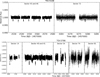 |
Fig. 1 PDCSAP from the TESS light curves for TOI-5108 (upper plot) and TOI-5786 (lower plot). For the last sectors for both targets where high cadence photometry is available, we show the 120 second cadence in grey and the flux data binned to the 10-minute cadence in black. |
2.2 Ground-based photometric follow-up
The TESS pixel scale is ~21″ per pixel and photometric apertures typically extend out to roughly 1′, generally causing multiple stars to blend in the TESS photometric aperture. To attempt to determine the true source of the TESS detections, we acquired ground-based time-series follow-up photometry of the field around TOI-5108 and TOI-5786 as part of the TESS follow-up observing program (TFOP; Collins 2019)1. We used the TESS Transit Finder, which is a customized version of the Tapir software package (Jensen 2013), to schedule our transit observations. All the light curve data are available on the EXOFOP-TESS website2. The light curves are shown in Figure A.1 and a summary of the observations is given in Table 1.
2.2.1 KeplerCam
TOI-5108.01 was observed on UT April 1, 2022, with Kepler-Cam on the 1.2m telescope at the Fred Lawrence Whipple Observatory (FLWO) at Mount Hopkins, Arizona. KeplerCam is a 4096 × 4096 Fairchild CCD 486 detector, which has a field-of-view of 23′ × 23′ and an image scale of 0.672″ per pixel when binned by 2. Data were reduced using standard IDL routines and aperture photometry was performed using AstroImageJ (Collins et al. 2017).
2.2.2 LCOGT
We observed a full transit window of TOI-5108.01 in Pan-STARRS ɀ-short band on UT December 20, 2023, from the Las Cumbres Observatory Global Telescope (LCOGT) (Brown et al. 2013) 1 m network node at McDonald Observatory near Fort Davis, Texas, United States (McD). The 1 m telescope is equipped with a 4096 × 4096 SINISTRO camera having an image scale of 0.389’’ per pixel, resulting in a 26′ × 26′ field of view. The images were calibrated by the standard LCOGT BANZAI pipeline (McCully et al. 2018), and differential photometric data were extracted using AstroImageJ.
Summary of the ground-based follow-up observations for TOI-5108 and TOI-5786.
2.2.3 MuSCAT2
We observed TOI-5108 and TOI-5786 with the multi-band imager MuSCAT2 (Narita et al. 2019) mounted on the 1.5 m Telescopio Carlos Sánchez (TCS) at Teide Observatory, Spain. MuSCAT2 is equipped with four CCDs and can obtain simultaneous images in ɡ′, r′, i′, and ɀs bands with little readout time. Each CCD has 1024 × 1024 pixels with a field of view of 7.4′ × 7.4′. All the MuSCAT2 data were reduced by the MuSCAT2 pipeline (Parviainen et al. 2019). The pipeline performs standard calibrations (dark and flat field corrections), aperture photometry, and transit model fit including instrumental systematics.
TOI-5786 was observed on UT July 14, 2023, and UT November 19, 2023. The TOI-5786 observations on the night of 14 July 2023 were made with nominal focus, and the exposure times were set to 5 s in all bands. The observations cover the full transit event, although with very little pre- and post-transit data.
The TOI-5786 observations taken on 19 November 2023 were made with the telescope defocused. The exposure times were set to 3 s in ɡ′, and 5 s in r′, i′, and ɀs, respectively. The full transit could not be observed, and the data cover the ingress with little pre-transit baseline.
TOI-5108 was observed with MuSCAT2 on the night of 26 December 2023. The observations were made with the telescope defocused and the exposure times were set to 15 seconds for all bands. The egress of the transit was detected.
2.3 High-angular-resolution imaging
We also collected high-angular-resolution imaging observations for both of our targets to search for unidentified close companions. These companions could dilute the transit signal leading to an underestimated radius for the planet (Ciardi et al. 2015) or (in the worst case) create false-positive scenarios if they happen to be eclipsing binaries.
We searched for stellar companions to TOI-5108 with speckle imaging on the 4.1-m Southern Astrophysical Research (SOAR) telescope (Tokovinin 2018) on 15 April 2022 UT, observing in Cousins I band, a similar visible bandpass as TESS. This observation was sensitive to a 5.3-magnitude fainter star at an angular distance of 1″ from the target. More details of the observations within the SOAR TESS survey are available in Ziegler et al. (2020). The 5σ detection sensitivity and speckle auto-correlation functions from the observations are shown in Figure C.1. No nearby stars were detected within 3’’ of TOI-5108 in the SOAR observations.
We observed TOI-5786 on November 8, 2022, UT and again on December 30, 2023, UT with the speckle polarimeter on the 2.5-m telescope at the Caucasian Observatory of Sternberg Astronomical Institute (SAI) of Lomonosov Moscow State University. The speckle polarimeter uses a high-speed, low-noise Hamamatsu ORCA-quest CMOS detector (Strakhov et al. 2023). Both observations were carried out in the Ic band, with an angular resolution of 0.083″ and seeing conditions of 0.6″ and 0.8″, respectively. The first observation revealed a companion at a separation of 1022 ± 9 mas, with a position angle (PA) of 238.3 ± 0.5 deg and a flux ratio of 0.0066 ± 0.0009 (Δmaɡ = 5.4 ± 0.2). In the second observation, the companion was detected at a separation of 1006 ± 9 mas, PA of 238.6 ± 0.5 deg, and flux ratio of 0.0086 ± 0.0016 (Δmaɡ = 5.2 ± 0.3). The sensitivity curves for both observations are shown in Figure C.1.
With the discovery of the companion to TOI5786 via speckle imaging, near-infrared adaptive optics imaging was obtained on July 29, 2024, UT with the PHARO instrument (Hayward et al. 2001) on the Palomar Hale (5m) in the Kcont (λo = 2.29; Δλ = 0.035 µm) and Hcont (λo = 1.668; Δλ = 0.018 µm) filters and on November 11, 2024, UT with NIRC2 on Keck II (10m) in the Jcont (λo = 1.2132; Δλ = 0.0198 µm) filter; both sets of observations were made behind the natural guide star systems (Wizinowich et al. 2000; Dekany et al. 2013). The PHARO pixel scale is 0.025″ per pixel and the NIRC2 pixel scale is 0.009942″ per pixel. Using a five-point quincunx dither pattern on Palomar and a three-point dither pattern on Keck, the reduced science frames were combined into a single mosaiced image with final resolutions of 0.09″, 0.07″, and 0.04″, at Kcont, Hcont, and Jcont respectively.
The sensitivity of the final combined AO image was determined by injecting simulated sources azimuthally around the primary target every 20° at separations of integer multiples of the central source’s FWHM (Furlan et al. 2017). The brightness of each injected source was scaled until standard aperture photometry detected it with 5σ significance. The final 5σ limit at each separation was determined from the average of all of the determined limits at that separation and the uncertainty on the limit was set by the rms dispersion of the azimuthal slices at a given radial distance. The Palomar and Keck imaging and sensitivities are shown in Figure C.1.
Given the flux ratio in the Ic band, which is closest to the TESS filter, we calculated the influence on the derived planet radius of TOI-5786.01. The potential error is less than 0.5% and much lower than other error sources (e.g., uncertainty on the stellar radius, scatter of the light curve). Therefore, we did not consider it in our analysis.
2.4 High-resolution spectroscopy
2.4.1 TRES
To assess the stellar properties and rule out eclipsing binary scenarios we obtained reconnaissance spectra with the Tillinghast Reflector Echelle Spectrograph (TRES, Furész et al. 2008) on the 1.5 m Tillinghast Reflector telescope at the Fred Lawrence Whipple Observatory (FLWO) on Mount Hopkins in Arizona. TRES is a fiber-fed, optical spectrograph with a resolving power of R = 44 000 covering the wavelengths between 390 and 910 nm. We obtained four spectra for TOI-5108 and two for TOI-5786.
For one of the TOI-5108 spectra, the observations were interrupted by clouds. All the spectra were visually inspected to check for composite spectra and then a multi-order spectral analysis was performed, following procedures outlined in Buchhave et al. (2010) and Quinn et al. (2012). Essentially, the spectra were cross-correlated order-by-order against a median combined template to derive the radial velocities. Then the spectra were corrected for zero-point offsets using a history of standard star observations. We found no signs of composite spectra or larger RV variations indicative of an eclipsing binary.
2.4.2 SOPHIE
To establish the planetary nature of the transit events, measure the masses of the companions, and constrain their orbits (in particular, the eccentricities), we observed both stars with SOPHIE. This stabilized échelle spectrograph is dedicated to high-precision radial-velocity measurements in optical wavelengths on the 193-cm Telescope at the Observatoire de Haute-Provence, France (Perruchot et al. 2008; Bouchy et al. 2009). It was already used to characterize several planetary candidates revealed by TESS (e.g. Moutou et al. 2021; König et al. 2022; Martioli et al. 2023; Serrano Bell et al. 2024). We used the high-resolution mode of SOPHIE (resolving power R = 75 000) and the fast reading mode of its CCD.
For TOI-5108 we secured 30 observations between February 2022 and March 2024. We excluded two of them due to low signal-to-noise ratio. For the 28 remaining exposures, the signal-to-noise ratio per pixel at 550 nm ranges from 28 to 52 (typically 40), for exposure times between 7 and 35 minutes (typically 15 minutes) depending on the weather conditions.
For TOI-5786, 15 observations were secured between April 2023 and March 2024. Signal-to-noise ratios per pixel and exposure times respectively range from 36 to 50 (typically 40) and from 12 to 36 minutes (typically 18 minutes), whereas one exposure was rejected due to its low signal-to-noise.
The radial velocities were extracted with the standard SOPHIE pipeline using cross correlation functions (CCF) as presented by Bouchy et al. (2009) and refined by Heidari et al. (2024). This includes in particular corrections for CCD charge transfer inefficiency, instrumental drifts, and pollution by Moonlight. The derived radial velocities have uncertainties of the order of 3 and 6 m/s, respectively for TOI-5108 and TOI-5786. For both objects, the radial velocities show significant variations in phase with the TESS ephemeris. The amplitudes of those variations indicate companions with masses in the planetary range. Additionally, the bisectors of the CCF were computed, and they show no correlations with the radial-velocity variations, as it might be the case if the transits are not due to planets but blended eclipsing binaries instead. The bisectors also constitute an activity indicator (see Sect. 3.3).
2.4.3 MaHPS
Together with the SOPHIE observations we also collected spectra with the Manfred Hirt Planet finder Spectrograph (MaHPS, Kellermann et al. 2015, 2016) consisting of the fiber-fed, high-resolution (R ~ 60000), optical (385-885 nm), echelle spectrograph FOCES (Pfeiffer et al. 1998), and a Menlo Systems Astro Frequency Comb as a wavelength calibration source.
MaHPS is mounted on the 2.1 m telescope at the Wen-delstein Observatory in southern Germany. It is temperature-and pressure-stabilized down to <0.01 K and <0.1 hPa inside an aluminum tank that is kept at an artificial overpressure (Fahrenschon et al. 2020). For the wavelength calibration, a Laser Frequency Comb (LFC) from Menlo Systems is used which produces narrow, regularly spaced emission lines between 470 and 740 nm. Two fibers are available with one recording the science light, while the other one is used to record the LFC spectrum for simultaneous wavelength calibration to correct for instrumental drifts during exposures (Brucalassi et al. 2016; Wang et al. 2017; Kellermann et al. 2019). Additionally, spectra of a Thorium-Argon (ThAr) lamp are recorded once every day before science observations for initial wavelength calibration. This calibration can also be used in case the precision of the comb is not needed or not available.
We acquired 141 MaHPS spectra on 48 observing nights between November 2022 and March 2024 for TOI-5108 and 113 spectra on 48 nights between May 2023 and April 2024 for TOI-5786. If possible we collected three 1800s exposures per night however, for some nights worsening weather conditions or higher priority observations meant we could only take one or two exposures. The observations in this paper belong to the first batch of science observations from the MaHPS spectrograph (see also Ehrhardt et al. 2024). Therefore the limiting observing conditions (e.g. weather, moon, seeing) were not well explored yet and some experimentation was done while observing the objects. This caused the number of spectra that were not suitable for precise RV work to be slightly higher compared to established spectrographs. In total, we have 120 spectra on 44 nights for TOI-5108 that are appropriate for precise RV analysis. For TOI-5786 we have 74 spectra on 35 nights. The first criterion for the evaluation of the spectra was the signal-to-noise ratio (S/N). We excluded data with an S/N less than 50% of the mean S/N for the target, which was mostly data affected by clouds. There were also cases where the filter of the LFC light was set to the wrong value (often after maintenance work on the LFC) which caused the LFC light to bleed into the target spectrum and introduced shifts in the RV. Lastly, there were observations where the targets were too close to the moon which caused contamination of the spectrum. In all of these cases, we excluded the affected observations from the analysis.
Additionally, there are nights for both stars where the frequency comb was down for maintenance or the comb flux was too low to be used for wavelength calibration. In both cases, only the wavelength for calibration from the ThAr lamp is used.
We developed two in-house software packages (GAMSE and MARMOT) to reduce the MaHPS spectra and calculate the radial velocities of the star. GAMSE (Wang et al. 2016) was used to reduce the raw data and extract 1D spectra. It also performs a preliminary wavelength calibration based on the ThAr spectra from the same day. MARMOT (Kellermann et al. 2020) then uses the 1D spectra and re-calibrates the wavelength solution based on the simultaneous LFC spectra. Next, it performs the barycenter correction using the Python package barycorrpy (Kanodia & Wright 2018) and masks any cosmic rays left in the spectrum. For the computation of the final RV shifts, MARMOT offers computation via the CCF method as well as the template matching method using a χ2 fit.
Stellar templates for the RV calculation in MARMOT were created from the individual observations through the simultaneous fitting of a cubic B-spline function. A separate template was created for each echelle order. First, the input spectra were scaled with a second-order polynomial and shifted by applying a multiplicative scaling to their wavelength axis to correct for shifts between the individual spectra and match them. In the following step, the χ2 statistic of the data points and the B-spline was minimized using the Python program iminuit (Dembinski et al. 2023), which is a python wrapper of the minuit minimizer. The final result is stored as a function to be evaluated during RV evaluation using either a CCF or χ2 fit.
For the templates of both stars, we used all observations that were left after the initial bad spectra rejection. We then derived the radial velocities for each order of the individual observations using the χ2 fitting routine in MARMOT. Before calculating the final radial velocities for each observation, we applied two corrections for known systematics in the MaHPS spectra.
The first known systematic offset in the MaHPS spectra are variations of the nightly zero-point (NZP) of the instrument. These variations have been common for many spectrographs and are often caused by instrumental events like detector or fiber changes (see Trifonov et al. 2020), fiber coupling problems, or thermal effects. For MaHPS the fiber coupling to the telescope is currently still in a provisional state, which can cause instabilities of the NZP. The NZP variations also seem to be correlated with sudden changes in the outside temperature, which could be propagated through the coupling of the science fiber to the telescope.
To correct for these nightly zero-point variations we observe one RV standard star between each TOI observation run. In total, we used four reference stars that are observable at different times throughout the year: HD185144, HD9407, HD221354, and HD89269. To build a nightly zero-point master that can be used to correct the science observations, we followed an approach that has been used for multiple other spectrographs (e.g., Courcol et al. 2015; Trifonov et al. 2018; Tal-Or et al. 2019). If we had multiple observations of a standard star for one night, we first binned them to avoid overweighting a particular star. Then we normalized the radial velocity measurements of each standard star by subtracting the error-weighted average of all their RV values. Lastly, the instrumental NZP is calculated by taking the error-weighted average RV of all RV standard stars that were observed on a given night.
In the case that we did not have the LFC available to correct for instrumental drifts during the night, we slightly altered our NZP calculation. Instead of calculating one zero-point for the whole night under the assumption that it should not change over the course of the observations, we used the reference star observations before and after each of the science exposures to correct for both the nightly zero point and the instrumental drifts during the exposures. In these cases, we interpolated between the reference star exposure before and after the science exposures and calculated a zero-point value for each exposure individually. We have found that this improves the precision of our RV measurements substantially for nights without the LFC, especially if there are strong variations in the temperature during the night. For the correction of the RVs of TOI-5108 and TOI-5786, the NZP value is subtracted from the RV value of each order for the respective nights.
A second systematic can be introduced during the template creation. Since the template is fitted for each order separately and the individual spectra are allowed to shift in wavelength, the templates of individual orders can have small offsets between each other. This can have an impact during the calculation of the final RV for the observations as we weigh the RV of each order by its error, which can unevenly amplify the effect of the template offsets. Therefore, after subtracting the NZP from the RV value of each order we normalized the orders to get rid of the offset by subtracting their error weighted average.
After applying both corrections to the order-wise RVs, we calculated the final radial velocities for each observation as the error-weighted average of the RVs from all spectral orders of the observation. The error of the radial velocity values is given by the weighted rms (see Zechmeister et al. 2018). Both the MaHPS and SOPHIE RVs that are used in the following analysis are available In Tables 8 and 9 at the CDS.
In addition to the RVs we computed activity indices from the calcium infrared triplet (IRT) lines following the definition of Kürster et al. (2003). We only used the first two lines of the IRT as the last line is located in the order that is cut off by the upper edge of the detector.
Stellar parameters from the analysis of the TRES, MaHPS, and SOPHIE spectra.
3 Stellar analysis
3.1 Spectroscopic stellar parameters
To characterize the two stellar hosts, we first extracted spec-troscopic stellar parameters from the observed TRES, MaHPS, and SOPHIE spectra. Stellar parameters from the TRES spectra are obtained by cross-correlating the spectra against Kurucz atmospheric models (Kurucz 1992) to derive stellar effective temperature, surface gravity, metallicity, and rotational velocity using the stellar parameter classification tool (SPC; Buchhave et al. 2012; Buchhave et al. 2014). We excluded the spectrum of TOI-5108 that was interrupted by clouds for the calculation of the average parameters. The average stellar parameters from the TRES spectra are shown in Table 2. We also used SPC to derive the rotational velocities for our two stars: υ sin i = 4.1 ± 0.5 km/s for TOI-5108 and υ sin i = 9.0 ± 0.5 km/s for TOI-5786.
For the MaHPS spectra, we compared the stellar templates that we created from our observations to a library of stars with precise and accurate Teff, log ɡ, and [Fe/H] values using the Python code SpecMatch-Emp (Yee et al. 2017). First, we normalized our MaHPS template and then fit it order-wise to the 404 library spectra in the wavelength range between 500 nm and 640 nm. The final parameters for our two stars are determined from a linear combination of the five best-fitting library spectra. In the case of TOI-5786, one of the five best-fitting stars had a significantly higher radius (2.2 R⊙ vs 1.2–1.5 R⊙) with a lower temperature (5600 K vs 6000–6300 K). For the linear combination of reference spectra, we remove this star and use the sixth best-fitting reference instead. While SpecMatch-Emp does not fit for the projected rotational velocity, v sin i, and does not include it in the final parameters, the reference stars often have measured v sin i values. For TOI-5108, the v sin i of the reference stars is between 2.3 and 4.2 km/s and, thus, close to the value derived from the TRES spectra. For TOI-5786, four of the reference stars have υ sin i between 6.6 and 7.4 km/s, with one outlier at a υ sin i of only 1.2 km/s.
For the SOPHIE spectra, we selected the ones without moonlight pollution and constructed an average spectrum for both stars. Following the method presented by Santos et al. (2013) and Sousa et al. (2021), we measured (for each averaged spectrum) the equivalent widths of selected iron lines and derived spectral parameters from them using the ARES+MOOG, including Teff, log ɡ, and [Fe/H]. The vsini values derived from SOPHIE are 3.3 ± 1.0 km/s and 7.0 ± 1.0 km/s, for TOI-5108 and TOI-5786, respectively. They were computed from the CCF parameters, using the calibrations of Boisse et al. (2010). The derived spectroscopic parameters are listed in Table 2. We used the weighted average of the values from the three spectrographs as priors on the spectroscopic stellar parameters in the following analysis to derive the bulk parameters of our two target stars.
3.2 Bulk stellar parameters
We then derived the bulk stellar parameters of both stars by analyzing their broadband spectral energy distribution (SED) with the Python package ARIADNE (Vines & Jenkins 2022). ARIADNE uses Bayesian model averaging to combine the results of fitting different stellar atmosphere models to account for and reduce model-specific systemic biases in the final parameters. For both stars, we used photometric data from the filters Johnson B, V, Gaia DR3 G, RP and BP, 2MASS JHK, and ALL-WISE W1 and W2 (W3 and W4 are not used as the PHOENIX V2 grid does not extend to that wavelength range) and included the GALEX NUV and FUV data for TOI-5108.
We convolved stellar atmosphere models from PHOENIX V2 (Husser et al. 2013), BT-Settl, BT-NextGen, BT-Cond (Hauschildt et al. 1999; Allard et al. 2012), Castelli & Kurucz (Castelli & Kurucz 2003), and Kurucz (Kurucz 1993) with the chosen filter bandpasses and interpolated them in Teff – log ɡ – [Fe/H] to fit to the photometric data.
The model for the SED includes six main parameters: the effective temperature Teff, the surface gravity of the star log g, the metallicity [Fe/H], the extinction Aυ and the stellar radius R* and distance D via the dilution factor (R*/D)2, which is used to obtain the observed fluxes from the theoretical grid fluxes (Casagrande & VandenBerg 2014). As an additional free parameter, an excess noise term ϵi for each photometric measurement is included.
We used a normally distributed prior around the Bailer-Jones distance estimate from Gaia EDR3 (Bailer-Jones et al. 2021) for the distance. The stellar radius and extinction are given flat priors ranging from 0.05 to 20 R⊙ for the radius and 0 to the maximum line-of-sight extinction calculated from the updated SFD galactic dust map (Schlegel et al. 1998; Schlafly & Finkbeiner 2011) through the dustmaps python package (Green 2018). For the parameters Teff, log ɡ and [Fe/H] we used the results from our spectroscopic analysis in Section 3.1 to impose Gaussian priors centered around the weighted average of the derived values.
Each stellar atmosphere model is fitted to the data separately and then the final values for all parameters are computed using a weighted average where the weights are given by the relative probability of the respective models. In the last step, the mass and age of the stars are estimated by comparing interpolated MESA Isochrones and Stellar Tracks (MIST, Dotter 2016; Choi et al. 2016) evolutionary models to the parameters derived from the SED fit using the isochrones (Morton 2015) software package.
As an independent confirmation of the stellar parameters we used the isoclassify package (Huber et al. 2017) to fit interpolated MIST and PARSEC (Bressan et al. 2012) isochrones directly to the broadband photometry and our derived spectroscopic parameters to model R*, M*, Aυ, L* and the stellar age. isoclassify has recently been used to homogenously derive a large sample of stellar properties from Kepler, K2, and TESS stars (Berger et al. 2020, 2023). We used the GAIA and 2MASS bands and imposed the same priors on the spectroscopic parameters that were used in the SED fitting. We first derived the luminosity directly from the bolometric flux and the GAIA parallax using the Bayestar19 (Green et al. 2019) reddening map for the extinction correction. This luminosity together with the spectroscopic constraints on Teff, log g and [Fe/H] is used to fit a grid of interpolated isochrones to derive the bulk stellar parameters. We perform this analysis for both the MIST and PARSEC isochrones.
The results of the SED (see Figure D.1) and the isoclassify fitting are shown in Table B.1. All three values agree within the errorbars. For the final stellar parameters in Table 3 we adopt the values from the isoclassify analysis with MIST isochrones as this approach was also used in a homogenous analysis of the TESS-Keck survey (MacDougall et al. 2023).
For the projected rotational velocity we adopt the values from SOPHIE spectra, which are also consistent with the expected values from the SpecMatch-Emp analysis of the MaHPS spectra. The rotational velocities derived from TRES are slightly higher, however, since the SPC does not take into account macroturbulence they can be slightly overestimated.
3.3 Stellar rotation period
From the projected rotational velocity v sin i, we can calculate an estimate for the rotational period of the target stars. Given the stellar radii from Table 3 we get Prot/ sin i = 20.0 ± 6.0 days for TOI-5108 and Prot/ sin i = 9.8 ± 1.4 days for TOI-5786. In theory, these are strict upper limits since the rotational velocity could be larger given an inclination of the stellar rotation axis <90°, however, measuring the rotational velocity of a star from the broadened spectra can be difficult as many other effects can broaden spectral lines (e.g., activity, turbulence), which are often difficult to model for the specific star. Underestimating these effects in the modeling can lead to an overestimation of the v sin i measured from the spectra translating into a larger range of possible rotational periods.
To further investigate the rotational period of the two stars, we constructed generalized-Lomb–Scargle (GLS, Zechmeister & Kürster 2009) periodograms from our RV data to search for any periodicities in the data that are not associated with our planetary signals. For both stars, the peaks with the highest power in the periodogram are associated with the period of the transiting planet. Therefore, we used the best-fit values of the periodogram to subtract the planetary signal. Figure 3 shows the periodogram of the RVs and the residuals. After subtracting the planetary signal there are no more signals above the false-alarm probability (FAP) threshold of 0.1%.
Additionally, we investigated the bisector of the CCF of the SOPHIE spectra and the first two lines of the calcium infrared triplet derived from the MaHPS spectra. We found no strong signals above a 0.1% FAP. Even below the FAP threshold, there are no distinct signals that are common in the RV residuals and the activity indicators. For TOI-5108 we found a peak close to the chosen FAP level in the RV residuals at 4.4 days and a couple of peaks in the two calcium lines at longer periods above 100 days. For TOI-5786 there are two distinct peaks in the SOPHIE bisector, one at the period of the planet and one at 8.2 days, which is close to the estimated rotational period from υ sin i.
Lastly, we checked the TESS light curves for signals of stellar activity. Due to the 2:1 resonance orbit of TESS and the Earth-Moon system, observations are subject to significant contamination from Earthshine and moonlight over the 13.7-day period. This effect and other systematics can severely hinder the detection of astrophysical signals. However, the applied corrections from SPOC can sometimes remove stellar signals in addition to instrumental systematics as both can occur on similar timescales. For cases where the expected rotational period is larger than 13.7 days, it can be better to use the SAP light curves to ensure that no stellar signals have been removed. However, this is only sensible if the light curves are not dominated by instrumental effects masking all stellar signals.
As the expected rotation period of TOI-5108 is larger than 13.7 days and the related SAP light curve is not dominated by systematics (see Figure 2), we used the SAP light curve for the periodogram analysis. For TOI-5786, the SAP photometry shows large instrumental effects and offsets for all sectors (see Figure 2). Given the large systematics in the SAP light curve and the fact that we expect the rotation period of TOI-5786 to be shorter than 13.7 days, we used the PDSCAP flux for the analysis. Since sectors 14 and 54 have large gaps in their PDCSAP data (see Figure 1) we only used sectors 40, 42, 74, and 81 for the Fourier analysis. In both cases, we masked out the transits before the analysis. The periodograms of the TESS data shown in Figure 3 are subject to strong aliasing due to the large gaps between the sectors. For TOI-5108, we found a forest of peaks around 15.2 days, while for TOI-5786 a similarly strong feature is seen around a period of 11.7days. As these results are close to the 13.7 day period of the spacecraft and there are clearly systematic effects still present in the data, it makes the interpretation of these signals difficult. We found no common features between the different datasets and also no significant signals in individual periodograms. Therefore, we were not able to constrain the stellar rotation period for either star with the available data.
Stellar parameters of TOI 5108 and TOI 5786.
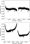 |
Fig. 2 SAP flux of TOI-5108 and TOI-5786. The lower plot shows the light curve of TOI-5786, which has strong systematics at the edges and an offset between the two sectors. For TOI-5108, the systematics are less severe (upper plot). |
3.4 Characterization of the TOI-5786 companion star
We performed a first characterization of the detected companion of TOI-5786 based on the Jcont, Hcont, and Kcont magnitudes. The magnitude differences of the two stars were measured with simple aperture photometry where the aperture radius was scaled to the FWHM of each image and sky radii were set to values outside the pair of stars. The magnitude differences are ΔJ cont = 4.022 ± 0.013 mag, ΔH cont = 3.743 ± 0.017 mag and ΔK cont = 3.413 ± 0.014 mag; the separation and position angle (EofN) of the companion relative to the primary star are 1.03 ± 0.01″ and 238.9 ± 0.2°.
Using the measured infrared magnitude differences, the unresolved 2MASS magnitudes have been deblended to retrieve real apparent magnitudes and infrared colors for the two stars. Based upon a 2MASS color-color diagram (Figure 4), the infrared colors of the stars are consistent with a late-type F-star (~F7V) for TOI-5786 (in agreement with the more detailed spectroscopic analysis of the star) and a mid-type M-star (~M5V), suggesting that the companion is a bound M-star. With a separation of 1.03 ± 0.01” and a distance of 193.8 ± 0.5 pc we calculated aprojected separation of 199.6 ± 2.1 au, which is sufficiently wide not to inhibit the 13-day orbital period of the planet.
4 Modeling the planetary systems
To derive the orbital and planetary parameters for our planet candidates we perform a joint analysis of our photometric and spectroscopic data using the python package juliet (Espinoza et al. 2019). juliet employs the batman package (Kreidberg 2015) to build the transit model for the photometry and radvel (Fulton et al. 2018) to build the Keplerian model for the RV analysis. For the fitting, juliet uses nested sampling algorithms that perform thorough sampling of the parameter space and at the same time allow for a comparison of different models via the difference in Bayesian evidence Δ ln(ɀ). In the following analysis, we used the dynamic nested sampling algorithm implemented via dynesty (Speagle 2020) to obtain the posterior distribution of the fitted parameters.
For both planets, the photometric data is modeled using the mid-transit time, T0, the orbital period, P, the impact parameter, b, and the planet-to-star radius ratio, Rp/R*. Instead of the scaled-semi-major axis, a/R*, we included the stellar density, ρ* as a fitting parameter, because it can be constrained from our stellar analysis. For the different photometric instruments, we included a jitter term for excess noise, σi, a relative flux offset, Mi and the quadratic limb-darkening parameters, q1 and q2, in the parametrization of Kipping (2013), which ensures that only values that are physically possible are explored in the sampling. As the reduction for our photometric data already includes a correction of possible contaminating sources we fixed the dilution factor of each instrument to 1. For the radial velocity data, we included a relative offset parameter, µi, and a jitter term, ωi, for each instrument in addition to the radial velocity amplitude, K.
For the eccentricity and the argument of periastron, we fit for  sin ω and
  , which has been shown to allow for fast, yet thorough sampling of the eccentricity (Eastman et al. 2013). This parametrization also mitigates the Lucy-Sweeney bias in the eccentricity measurement (Lucy & Sweeney 1971). We use the stellar parameters derived in Section 3 to impose Gaussian priors on both the stellar density and the limb-darkening parameters for the TESS light curves. The mean of the density prior is calculated from the stellar masses and radii from Table 3 with the derived error as the variance.
Limb-darkening parameters for our photometric data are calculated using the Synthetic-Photometry/Atmosphere-Model (SPAM) method of Howarth (2011). In this approach, synthetic light curves are created with an accurate representation of the stellar intensity profile through the use of theoretical limb-darkening coefficients derived from the non-linear law and assuming full knowledge of the planetary and stellar properties. These synthetic light curves are then fitted with all parameters fixed except for the desired limb-darkening law. This has been shown to minimize the difference between theoretically and empirically derived limb-darkening parameters (Patel & Espinoza 2022).
We used the ExoCTK package (Bourque et al. 2021) to compute both, the nonlinear limb-darkening coefficients for the synthetic input light curves from PHOENIX stellar atmosphere models and the final SPAM coefficients from the quadratic law (u1 and u2) to be used in the fitting of the orbit. The two quadratic limb-darkening coefficients are then transformed to q1 and q2 via the relations given by Kipping (2013). The other parameters are given uniform priors with the period and transit mid-time bounds being relatively tightly centered around the predicted values from the TESS light curves to be more efficient in the sampling.
For each planet, we performed multiple fits with different models and compare them using the Bayesian evidence (ln Z). A Δ ln Z > 2 between two models constitutes a moderate preference for one model over the other, while a Δ ln Z > 5 indicates a strong preference (Trotta 2008).
In particular, we are interested in two quantities when comparing models: the eccentricity of the orbit and the presence of other signals either through unaccounted systematics, stellar activity, or other planets in the system. To investigate whether the data for the two planets warrants an eccentric orbit we perform two separate fits for each planet. In one fit the eccentricity, e, and the argument of periastron ω are fixed to 0 and 90°, respectively and in the other, both parameters are allowed to vary freely. We then use the Bayesian evidence to compare the two models and determine whether the data warrants an eccentric solution for the orbit.
Additionally, we attempted to model any remaining systematics and possible effects of stellar activity in our data using Gaussian process regression (GP, see e.g. Aigrain & Foreman-Mackey 2023). For this, juliet employs multiple different GP Kernels via the george (Ambikasaran et al. 2015) and celerite (Foreman-Mackey et al. 2017) packages. While Gaussian process regression can be a powerful tool to recover small planetary signals and measure precise masses in the presence of noise from stellar activity (Barragán et al. 2019, 2023; Mantovan et al. 2024), one has to be careful not to overfit the data, which can in turn lead to masking or altering of the planetary signals (Ahrer et al. 2021; Rajpaul et al. 2021; Blunt et al. 2023). Therefore, in the following analysis, we are careful to only apply GP where the data warrant it.
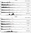 |
Fig. 3 GLS periodograms of TOI-5108 and TOI-5786. The top periodograms belong to TOI-5108. The first and second rows are the RV data from MaHPS and SOPHIE before and after subtracting the signal of the transiting planet. The next three rows show the periodograms of the activity indicators derived from the SOPHIE spectra (BIS) and MaHPS spectra (Ca IRT). The last row shows the periodogram of the TESS data. The dotted red line shows the period of the transiting planet and the dotted black line is located at the 0.1% FAP. Bottom periodograms are the same as the top ones but for TOI-5786. |
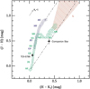 |
Fig. 4 Spectral type classification of TOI-5786 and the detected companion. Using the AO imaging, the 2MASS magnitudes have been deblended and the two stars have been placed on a JHKs color–color diagram. |
4.1 TOI-5108
We derived the orbital parameters for the companion of TOI-5108 by using a joint fit of the radial velocities from MaHPS and SOPHIE and the photometry of TESS together with the Kepler-Cam, LCOGT, and MuSCAT2 transits. As the SPOC pipeline already detrends the TESS data and there are no signs of significant remaining systematics we do not include a GP kernel on the TESS data.
We performed two fits once to a circular and once to an eccentric model for the orbit of TOI-5108 b on the combined dataset. The difference between the Bayesian log evidence is 7 in favor of the circular model.
Early in the observations, the data showed a slight trend especially in the MaHPS observations but also between the 2022 and 2023 SOPHIE observations (although in 2022 only one observation was taken). The trend got weaker with the addition of the 2024 observations. Nevertheless, we investigated the presence of another planet in our data with another fit where we have broad uniform priors for the period, T0, and the RV amplitude. The two-planet fit is strongly disfavored compared to the one-planet models with a Δ ln Z of 7.
As a consistency check, we also compared the derived RV amplitudes when only one of the spectroscopic datasets is used. The RV amplitude from the MaHPS spectra (12 ± 2 m/s) is consistent with the one derived from SOPHIE (8.4 ± 1.9 m/s).
The final values for the properties of the planet around TOI-5108 adopting the values of the circular model are shown in Table 4 and a plot of the phase-folded RV and time-series are shown in Figure 5.
4.2 TOI-5786
4.2.1 Light curve analysis
As mentioned in Section 3.3, the PDCSAP light curve for TOI-5786 shows some variation stemming from uncorrected systematics as well as potential stellar activity. As some of these variations occur close to transits, this could influence the measured transit depth and thus the derived planetary radius. To mitigate this issue, we included different GP Kernels in the fitting to detrend the TESS data. We chose three GP Kernels with varying degrees of freedom. The first Kernel is the Matern kernel parametrized in celerite with an amplitude (σGP) and a time/length scale (ρGP). This Kernel is very versatile and frequently used to model both long-term trends and short-term stochastic variations. The other two kernels are the simple harmonic oscillator (SHO) and the quasi-periodic kernel (QP), which have both been shown to be able to reproduce the quasi-periodic oscillations associated with stellar activity quite well (see e.g., Ribas et al. 2018; Nicholson & Aigrain 2022). Details on all three kernels are given in Foreman-Mackey et al. (2017).
In the first step, we used the TESS light curves to fit a transit model, including the known TESS candidate planet with the GP kernels, and evaluated which configuration was preferred by our data. The Bayesian evidence values of the different fits are given in Table 5. There is a clear preference for the inclusion of a GP kernel, with all three GP fits having much higher evidence values than the fit without a GP kernel. Among the three Kernels, the preferred one is the quasi-periodic Kernel with a strong preference (ΔZ > 5) over the other two.
We also searched for additional planet candidates in the system with the Open Transit Search pipeline (OpenTS; Pope et al. 2016) using the sectors 14, 40, 41, and 54 produced by the TESS-SPOC pipeline. This analysis identified a significant transit-like signal with a period of 6.99 d that had not been reported as a TOI by the TESS mission. This planet candidate was independently detected by the Planet Hunter TESS initiative (Eisner et al. 2020) and was reported as a community TOI (CTOI) on EXOFOP.
To investigate the presence of the second planet further, we fit models including the second planet to our light curves and compared the Bayesian evidence. We run the two-planet fit twice, once with normal priors on P and T0 from the BLS analysis and once with uniform priors between 1 and 10 days for the period and 2458680 BJD and 2458690 BJD for the mid-transit time. The two-planet model is heavily favored over the one-planet model (ΔZ > 50) for all cases even with uniform priors and no GP correction. Figure 6 shows the TESS light curve with the best fitting GP + transit model as well as the phase folded transit light curves of the two potential planets.
4.2.2 Combined fitting
To derive the system’s final parameters, we performed a joint fit of the MaHPS and SOPHIE radial velocities together with the photometry from TESS and the two observed transits of MuSCAT2. The priors for all parameters are shown in Table 6. As both MuSCAT2 transit observations only included very little baseline, we fixed the limb-darkening parameters to their theoretical values since it would be difficult to constrain them well from the data. For the TESS data, we included the quasi-periodic GP kernel. We also tested whether applying the QP kernel to our RV data is warranted but found such models to have a lower Bayesian evidence value compared to the ones that do not include a GP kernel on the RVs. This further supports the assumption that the GP is mainly modeling systematics in the TESS data and not underlying stellar processes, which would be present in both datasets.
As with TOI-5108, the fit was performed once for a circular and once for an eccentric orbit. In our results, the circular orbit is strongly favored with a Δ ln Z of 24. Therefore, we adopted the values from the circular fit for the final parameters shown in Table 6. We were not able to measure the mass of the inner planet. However, from the fit, we derived a 3-σ upper limit for the radial velocity amplitude of 10.0 m/s. As a consistency check, we also ran the one-planet model on the combined dataset but found that the Bayesian evidence was much lower (Δ ln Z > 100 in favor of the two-planet model). The derived values of the orbital parameters of TOI-5786.01 are also consistent within 1σ between the one-planet and the two-planet model. Furthermore, the RV amplitudes between a MaHPS-only and a SOPHIE-only fit are again consistent within the errors (19 ± 4 m/s vs 16 ± 3 m/s). Figure 7 shows the RV time series with the Kep-lerian model of both planets and the phase-folded RV of the outer planet.
Priors and final parameter values from the juliet fit of TOI-5108.
Bayesian evidence values for the different GP models fitted to the TESS data of TOI-5786.
4.2.3 Photodynamical modeling
We carried out a photodynamical analysis modeling the TESS photometry and the MaPHS and SOPHIE radial velocities jointly using PyTTV as described in Korth et al. (2023) to see whether we could constrain the inner planet’s parameter further when accounting for gravitational interaction between the two planets. The code models the observations simultaneously using rebound (Rein & Liu 2012; Rein & Spiegel 2015; Tamayo et al. 2020) for dynamical integration and PyTransit (Parviainen 2015, 2020; Parviainen & Korth 2020) for transit modeling, and provides posterior densities for the model parameters estimated using MCMC sampling in a standard Bayesian parameter estimation framework. The photodynamical modeling gives a smaller upper mass limit of 26.5 M⊕, and supports small eccentricities for both planets, with 95th posterior percentiles of 0.07. The analysis also predicted measurable transit timing variations (TTVs) for both planets. For the inner planet, amplitudes up to 20 min, and for the outer planet, up to 3 min are predicted. However, the sparse sampling of the transit observations combined with low S/N compared to the expected TTV amplitudes prevents a secure TTV detection in the observed photometry.
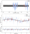 |
Fig. 5 Result of the juliet fit of TOI-5108. Upper panel: radial velocity curve of TOI-5108 with the best fit Keplerian model for TOI-5108 b in black. Middle panel: phase-folded radial velocity curve. The dark blue data points represent the MaHPS RV data binned at 0.05 phases. Light blue is the unbinned MaHPS data and red is the SOPHIE data. Lower Panel: Residuals after subtracting the signal of TOI-5108 b. |
5 Results and discussion
5.1 Planetary parameters of the two sub-Saturns
We have established the planetary nature of the two TESS candidates, which we refer to as TOI-5108 b and TOI-5786 b here. Their position among the population of known transiting exo-planets is shown in Figure 8. TOI-5108 b is a sub-Saturn sized planet with a radius of 6.6 ± 0.1 R⊕ and a mass of 32 ± 5 M⊕ orbiting its host star with a 6.753 day period. With the planet being this close to the host star (a = 0.073 ± 0.004 au) it is located inside the bounds of the Neptune desert as defined by Mazeh et al. (2016). Depending on the XUV radiation of its host star the planet may experience significant mass loss via atmospheric escape although it is not in the very barren region of the desert (P < 3 days) where the escape is expected to be strongest. TOI- 5786 b is located outside the desert with a period of 12.779 days and a radius of 8.54 ± 0.13 R⊕. Given the mass of the host star derived in Section 3.2 we calculate a planet mass of 73 ± 9 M⊕.
The newly detected planet candidate around TOI-5786 is also shown in Figure 8. With a period of 6.99 days and a radius of 3.83 ± 0.16 R⊕, it would be a sub-Neptune at the lower boundary of the Neptune desert. We derive 3-σ upper limits for the mass of the planet candidate of 34 M⊕ from the Keplerian fit to the RVs and 26.5 M⊕ from the photodynamical modeling. These masses translate into a density upper limit of 3500 kg/m3 indicating the presence of a volatile-rich atmosphere as expected from the larger radius. Both sub-Saturns have bulk densities similar to Saturn at 600 ± 90 kg/m3 (TOI-5108 b) and 640 ± 80 kg/m3 (TOI- 5786 b). This implies that a significant portion of the planet’s mass is contained in a H/He envelope.
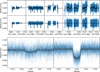 |
Fig. 6 TESS light curve of TOI-5786 before and after the GP correction. Top row: TESS light curve of TOI-5786 with the GP + transit model. Middle row: TESS light curve with the GP model subtracted showing only the transits of the two planet candidates. Bottom row: phase-folded lightcurves of the TESS Object of Interest TOI-5786.01 on the right and our detected planet candidate on the left. |
5.2 Envelope fractions
For sub-Saturns, both the rocky core and the H/He envelope contribute to the planet’s mass budget. As the detailed composition of the core is assumed to only have a small effect on the overall mass fractions, it is possible to constrain the envelope and core mass fractions using simple two-component models (Lopez & Fortney 2014; Petigura et al. 2016, 2017). We used the Python code Platypos (Poppenhaeger et al. 2021) to estimate the internal structure and evolution of the two planets. The code first calculates the envelope fraction, fenv, based on the models of Lopez & Fortney (2014). Then it estimates the evolution of the planetary envelope given the age of the system based on energylimited hydrodynamic atmospheric escape models (see Eq. (1) in Poppenhaeger et al. 2021) given the X-ray and extreme UV (XUV) irradiance of the planet.
We estimated the X-ray luminosities of our two host stars from the relations between X-ray luminosity, stellar mass, and rotation period given in Pizzolato et al. (2003). This results in luminosities of ( ) × 1028 erg s−1 for TOI-5108 and (
 ) × 1028 erg s−1 for TOI-5786.
Given this X-ray luminosity and the planetary and stellar parameters derived in this work, Platypos estimates a presentday envelope fraction of ~38% for TOI-5108 b and ~74% for TOI-5786 b. Prevailing planet formation theory assumes that runaway accretion starts at fenv ~ 50%, which would mean that TOI-5786 b was able to incite runaway accretion while the formation of TOI-5108 b was finished shortly before. Planets with estimated envelope fraction close to 50% such as K2- 19 b (Petigura et al. 2020) or K2-24 c (Petigura et al. 2018a) have posed a challenge to the prevailing theory of the onset of runaway accretion.
One proposed solution by Millholland et al. (2020) includes tidal heating in the model which lowers the derived envelope fractions to be more aligned with expectations from theory. Based on our analysis, TOI-5108 b does not appear to have any significant eccentricity in its orbit; however, the obliquity of the planet is unknown and a non-zero axial tilt can also cause tidal heating. We therefore used the model from Millholland et al. (2020) to calculate the envelope fraction of TOI-5108 b including tidal heating3. The strength of the reduction of the envelope fraction after the inclusion of tidal forces depends on the obliquity of the orbit and the tidal quality factor Q′. Based on our Solar System and exoplanets with measured tidal quality factors, Q′ ~ 104–105 is a realistic estimate for this parameter (Murray & Dermott 1999; Zhang & Hamilton 2008; Morley et al. 2017; Puranam & Batygin 2018). In Figure 9, we show the results of the derived envelope fraction for TOI-5108 b as a function of Q′ for different obliquities. Without the inclusion of tides, the envelope fraction is similar to the one calculated with Platypos at 38.6 ± 2.4%. With tides, this drops to between 10–20% depending on the obliquity λ and Q′ . At these envelope fractions, the internal and atmospheric structure of TOI-5108 b would likely be more similar to a sub-Neptune than a gas giant.
The expected amplitude of the Rossiter McLaughlin (RM) effect for TOI-5108 is ~5 m/s. As such it will be possible to measure the obliquity of TOI-5108 b with existing high-resolution spectrographs although a larger mirror size than the size of the telescopes used in this paper is preferable to get a better time sampling during the transit.
Priors and final parameter values from the juliet fit of TOI-5786.
5.3 Future characterization possibilities
Using Eq. (1) from Kempton et al. (2018), we calculated the Transmission Spectroscopy Metric (TSM) of both planets to assess whether they are favorable targets for atmospheric characterization with JWST. The TSM is a measure for the expected S/N of a JWST transit observation given the properties of the host star and the expected strength of spectral features in the planet’s atmosphere.
We calculated the TSM values of 138 ± 25 and 78 ± 12 for TOI-5108 b and TOI-5786 b, respectively. For sub-Jovian planets, Kempton et al. (2018) found a threshold of 90 for a planet to be considered a high-quality follow-up target for JWST making TOI-5108 b a good target to further investigate the atmospheric composition of these intermediate-sized planets. While TOI-5786 b is slightly below this threshold, among the subSaturns with longer periods (P < 10 days) and precise masses and radii, it is in the top 20% of the highest TSM making it a solid target for further study in the slightly longer period regime.
Due to its position in the Neptune desert, one point of interest for an atmospheric follow-up of TOI-5108 b would be to search for signs of an escaping atmosphere. Atmospheric escape through photoevaporation is one of the proposed mechanisms that could result in a dearth of short-period, intermediate-sized planets. As TOI-5786 b is located a bit farther away from its host star and also slightly more massive, the mass loss through atmospheric escape is expected to be slightly weaker.
Using the open source code p-winds (Dos Santos et al. 2022), we investigate whether ongoing atmospheric escape would be detectable through transmission spectroscopy using the metastable triplet Helium line as a tracer. Based on the planetary parameters and an XUV spectrum of the host star, p-winds calculates the ionization fraction of hydrogen and helium and then models the atmospheric escape with a one-dimensional Parker wind model (Parker 1958; Oklopčić & Hirata 2018). It then estimates the strength of the absorption from the metastable triplet helium at 1083 nm during transit.
Since the XUV spectra of TOI-5108 and TOI-5786 are unknown, we use measured spectra from similar stars as proxies.
To cover a range of XUV luminosities we use HD 108147, the sun, and WASP 17 as proxies of low, medium, and higher stellar activity respectively. The spectra of HD 108147 and WASP 17 are taken from the MUSCELS survey (Loyd et al. 2016; Youngblood et al. 2016; France et al. 2016; Behr et al. 2023). Due to the older age, TOI-5108 b is likely more similar to the Sun or HD 108147 while the younger age and shorter rotation period point to TOI-5786 having a higher activity.
We first estimate the mass-loss rate of both planets based on the integrated XUV flux of our three proxy spectra with a simple energy-limited hydrodynamic escape model (Watson et al. 1981; Lopez et al. 2012; Owen & Jackson 2012), following the assumption of Foster et al. (2022) who calculated atmospheric escape rates from eROSITA data. The mass-loss rate is given by:
 1
1
where ϵ is an efficiency parameter set to 0.15, G is the gravitational constant, Rp and Mp are the planetary radius and mass, FXUV is the X-ray and extreme-UV flux incident on the planet and RXUV is the planetary radius at XUV wavelengths (assumed to be 1.1 times the optical radius); Ktide is the reduction factor of the planetary gravitational potential due to the effect of a stellar tide, which we assume to be negligible.
Table 7 shows the integrated XUV flux and corresponding mass-loss rates of both planets for the three XUV spectra. We use the estimated mass-loss rates, XUV spectra, and the planetary and stellar parameters as input for p-winds to calculate the expected absorption in the triplet helium during transit assuming a hydrogen fraction of 0.9 and a thermospheric temperature of 7000 K. Next we simulate an observation with JWST NIRSpec G140H (R ~ 2700) using PandExo (Batalha et al. 2017) to check whether the signal would be observable. As shown in Figure 10, even in the case of the strongest XUV flux, the helium signal is not detectable in the NIRSpec data. Due to the lower mass-loss rates and the suboptimal stellar types with regards to the triplet helium feature (see Oklopčić 2019) the absorption signal is too weak to be detectable.
Lastly, with the mass-loss rates from Table 7 and the envelope fractions of Section 5.2 we can calculate the time it would take for the planets to lose their atmospheres. This yields 288 ± 50 Gyrs for TOI-5786b and 24 ± 6 Gyrs for TOI-5108b in the highest mass-loss scenario showing that both planets are presently stable against photoevaporation.
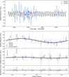 |
Fig. 7 Results of the juliet fit of TOI-5786. First panel: radial velocity curve of TOI-5786 with the best fit Keplerian model for the two-planet case in black. Second panel: RVs phase-folded to TOI-5786 b. The dark blue data points represent the MaHPS RV data binned at 0.05 phases. Third Panel: RVs phase-folded to the period of the inner companion candidate. Fourth Panel: Residuals after subtracting the signals of both planets. |
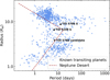 |
Fig. 8 Population of known transiting exoplanets with masses and radii measured to 33% or better taken from the NASA Exoplanet Archive (accessed on 14.10.2024). TOI-5108 b and TOI-5786 b are shown with black stars. The position of the planet candidate around TOI-5786 is shown with a white star. The dotted brown line indicates the boundaries of the Neptune desert as defined by Mazeh et al. (2016). |
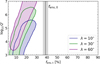 |
Fig. 9 Estimate of the envelope mass fraction, fenv, of TOI-5108 b using the model from Millholland et al. (2020). The grey bar is the calculated envelope fraction with the associated error in the tides-free model. The shaded regions show the 2-σ contours of the envelope fraction for different obliquities, λ. |
X-ray and EUV fluxes and the corresponding mass-loss rates derived from the three proxy spectra for both planets.
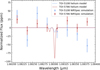 |
Fig. 10 Simulated transit observation with NIRSpec for the helium triplet absorption signals calculated with p-winds. The helium absorption models shown are for the high XUV input spectrum (WASP-17) with the largest mass-loss rates. |
5.4 False positive tests for the second transit signal around TOI-5786
From our RV data, we were not able to detect the potential inner planet around TOI-5786 as the errors on the SOPHIE and especially the MaHPS data much are larger than the expected RV amplitude from the inner planet (~3 m/s).
To further validate the signal as a planet, we perform several false-positive tests on the TESS data. First, we split the transit dataset into odd and even transits to investigate whether there is a difference in transit depth indicative of an eclipsing binary configuration. We find transit depths of 1063 ± 60 ppm for the odd transits and 1058 ± 90 ppm for the even transits. These depths agree well within the uncertainties indicating a consistent transit depth between the odd and even transits.
Next, we investigate the source of the transit event by looking at the difference images between the out-of-transit and the in-transit flux created from the target pixel files that are created by the SPOC. Due to the low signal-to-noise of the individual transits the pixel with the highest flux difference is not always associated with TOI-5786. For multiple transits, the pixel with the highest difference in flux before and during the transit is close to TIC 40292668. However, a visual inspection of the light curve of TIC 40292668 shows no transit events that coincide with the transit signal of the potential inner planet of TOI-5786. Furthermore, the light curve of TIC 40292668 shows some variability, which could explain the offset of flux difference images.
Lastly, we use the statistical validation tool TRICERATOPS (Giacalone & Dressing 2020; Giacalone et al. 2021) to estimate the false-positive probability of our transit signal. TRICERATOPS is a Bayesian tool that compares the derived light curve to a wide range of possible transit-producing events, taking into account the used aperture as well as knowledge of the target star and its surrounding stars from GAIA to calculate a false positive probability (FPP) and a nearby false positive probability (NFPP). We use data from all available sectors for TOI-5786 to produce a phase-folded light curve, which we use as an input for the analysis. First, we calculate the S/N of our transits using Equation (17) of Giacalone et al. (2021) to assess whether the derived FPP and NFPP from Triceratops are reliable. We get an S/N of 30, which is above the threshold of 15 for reliable results as found in Giacalone et al. (2021). We run TRICERATOPS 20 times and derive an average FPP of 0.030 ± 0.004 and a NFPP of 0.0154 ± 0.0014. The bulk of the NFPP probability is caused by TIC 40292668 (an average of 0.14) which does not show any obvious transit events in its light curve. While these probabilities are rather low, they are not enough to statistically validate the planet according to Giacalone et al. (2021) (FPP < 0.015 and NFPP < 10−3).
Since we detected a secondary star close to TOI-5786 through our high-resolution imaging observations we consider the scenario where the second planet is orbiting this star. Given the magnitude difference between the two stars (~5.3 mag) in the Ic filter and the measured transit depth on TOI-5786 of 690 ppm, the depth on the secondary star would need to be ~9% making it most likely a giant planet or brown dwarf transiting the M star. The TRICERATOPS probability for a blended eclipsing binary or planet transit on a blended star is rather low (0.015 ± 0.004 adding the different blended scenarios). To further investigate this possibility we fit the TOI-5786 light curve with single-planet models for TOI-5786 b and for the second planet candidate. In this fit, we impose a uniform prior on the stellar density. We can then compare the derived densities to the stellar density from Section 3 to asses which star is more likely to host each planet (see Lester et al. 2022). The derived density for the transit fit of TOI-5786 b is  kg/m3, which is similar to the depth derived from the transit fit of the second planet candidate at
  kg/m3 . Both densities agree well with the value derived in Section 3 of 690 ± 80 kg/m3 . We therefore conclude that it is unlikely, that the second transiting signal happens on the blended stellar companion.
6 Conclusions and summary
We have detected and measured precise masses for the new transiting planets TOI-5108 b and TOI-5786 b. The planets are sub-Saturns, with radii of 6.6 ± 0.1 R⊕ and 8.54 ± 0.13 R⊕, and masses of 32 ± 5 M⊕ and 73 ± 9 M⊕, respectively. Additionally, we found a signal of another transiting planet in the TESS light curve of TOI-5786. This potential planet would be an inner companion to TOI-5786 b, with a period of 6.99 days and a radius of 3.83 ± 0.16 R⊕. With a period of 6.573 days, TOI-5108 b is located inside the bounds of the Neptune desert; whereas TOI- 5786 b, with a period of 12.779 days, is located at the upper edge.
The metallicity of TOI-5108 ( ) suggests that the envelope of TOI-5108 b could be metal-. rich, which would have helped the planet retain a large fraction of its atmosphere against photoevaporation during its early lifetime, due to the enhanced cooling from atomic metal lines. TOI-5108 b follows the trend of hot super-Neptune-sized planets preferably occurring around metal-rich stars. Even TOI-5786 has a slightly higher metallic- ity, although it is consistent with solar metallicity within the uncertainty.
TOI-5108 b and TOI-5786 b have envelope mass fractions slightly below and above the runaway accretion limit at ~38% and ~74%, respectively. As both planets have high TSM values, an in-depth study of their respective atmospheres could be helpful in looking for differences in the composition of planets that have been able to incite runaway gas accretion and planets whose formation had ceased at an earlier stage.
From our analysis, we find that both planets are likely stable against photoevaporation. However, our calculation of the massloss rates is based on proxy spectra, so a direct measurement of the mass-loss rates through transmission spectroscopy is needed to draw definitive conclusions. Even if the mass-loss signature is not detectable as predicted from our simulations, an upper limit on the mass-loss rate could be used to confirm the assumption of stability against photoevaporation.
The stability of the two planets against photoevaporation further strengthens the assumption that the upper edge of the Neptune desert is caused by a different mechanism, such as high-eccentricity migration. Interestingly, an inner companion for TOI-5786 b would reduce the likeliness of high-eccentricity migration as a realistic mechanism explaining its present-day orbit. Such a planetary system would likely form through a more quiet mechanism, such as disk migration. This does not necessarily conflict with the assumption that the upper edge of the Neptune desert is formed by high-eccentricity migration because TOI-5786 b is not located directly at the desert boundary.
Data availability
Tables 8 and 9 are available at the CDS via anonymous ftp to cdsarc.cds.unistra.fr (130.79.128.5) or via https://cdsarc.cds.unistra.fr/viz-bin/cat/J/A+A/694/A143. The tables contain the following information: column 1 lists the time of the observations, column 2 gives the derived RV values, column 3 gives the error of the RV, and column 4 lists the name of the instrument.
Acknowledgements
We thank the anonymous referee for the corrections and suggestions that helped us improve the presentation of the paper. We want to acknowledge the independent detection of the inner planet around TOI-5786 by the Planet Hunter TESS team including Sam Lee, Hans Martin Schwengeler, Cledison Marcos da Silva, Simon Lund Sig Bentzen, Kim Donghyeon, Safaa Alhassan, Ciaron Drain, Marc Huten, Roberto Gorelli, Allan Tarr, Ian R. Mason and Nora Eisner. We note that they also found two more potential transit events that are not associated with the two planets. However, as these events are separated by 1634 days and the period cannot be determined they are not considered in our analysis. LT acknowledges support from the Excellence Cluster ORIGINS funded by the Deutsche Forschungsgemeinschaft (DFG, German Research Foundation) under Germany’s Excellence Strategy – EXC 2094 – 390783311. The Wendelstein 2.1 m telescope project was funded by the Bavarian government and by the German Federal government through a common funding process. Part of the 2.1 m instrumentation including some of the upgrades for the infrastructure were funded by the Cluster of Excellence “Origin of the Universe” of the German Science foundation DFG. We thank the Observatoire de Haute-Provence (CNRS) staff for its support. This work was supported by the “Programme National de Planétologie” (PNP) of CNRS/INSU and CNES. Funding for the TESS mission is provided by NASA’s Science Mission Directorate. KAC and CNW acknowledge support from the TESS mission via subaward s3449 from MIT. We acknowledge the use of public TESS data from pipelines at the TESS Science Office and at the TESS Science Processing Operations Center. Resources supporting this work were provided by the NASA High-End Computing (HEC) Program through the NASA Advanced Supercomputing (NAS) Division at Ames Research Center for the production of the SPOC data products. This paper includes data collected by the TESS mission, which are publicly available from the Mikulski Archive for Space Telescopes (MAST) operated by the Space Telescope Science Institute (STScI). This research has made use of the Exoplanet Follow-up Observation Program (ExoFOP; DOI: 10.26134/ExoFOP5) website, which is operated by the California Institute of Technology, under contract with the National Aeronautics and Space Administration under the Exoplanet Exploration Program. This work makes use of observations from the LCOGT network. Part of the LCOGT telescope time was granted by NOIRLab through the Mid-Scale Innovations Program (MSIP). MSIP is funded by NSF. We acknowledge financial support from the Agencia Estatal de Investigación of the Ministerio de Ciencia e Innovación MCIN/AEI/10.13039/501100011033 and the ERDF “A way of making Europe” through project PID2021-125627OB-C32, and from the Centre of Excellence “Severo Ochoa” award to the Instituto de Astrofisica de Canarias. This article is based on observations made with the MuSCAT2 instrument, developed by ABC, at Telescopio Carlos Sánchez operated on the island of Tenerife by the IAC in the Spanish Observatorio del Teide. This work is partly financed by the Spanish Ministry of Economics and Competitiveness through grants PGC2018-098153- B-C31. This work is partly supported by JSPS KAKENHI Grant Numbers JP24H00017, JP24H00248, JP24K00689, JP24K17082 and JSPS Bilateral Program Number JPJSBP120249910. This research has made use of the NASA Exoplanet Archive, which is operated by the California Institute of Technology, under contract with the National Aeronautics and Space Administration under the Exoplanet Exploration Program. S.G.S acknowledges the support from FCT through Investigador FCT contract nr. CEECIND/00826/2018 and POPH/FSE (EC). A.A.B. and I.A.S. acknowledge the support of M.V. Lomonosov Moscow State University Program of Development. DRC acknowledges partial support from NASA Grant 18-2XRP18_2-0007. Based on observations obtained at the Hale Telescope, Palomar Observatory, as part of a collaborative agreement between the Caltech Optical Observatories and the Jet Propulsion Labora- tory(operated by Caltech for NASA). This work was supported by a NASA Keck PI Data Award, administered by the NASA Exoplanet Science Institute. Data presented herein were obtained at the W.M. Keck Observatory from telescope time allocated to the National Aeronautics and Space Administration through the agency’s scientific partnership with the California Institute of Technology and the University of California. The Observatory was made possible by the generous financial support of the W.M. Keck Foundation. The authors wish to recognize and acknowledge the very significant cultural role and reverence that the summit of Maunakea has always had within the indigenous Hawaiian community. We are most fortunate to have the opportunity to conduct observations from this mountain. This research was carried out in part at the Jet Propulsion Laboratory, California Institute of Technology, under a contract with the National Aeronautics and Space Administration (80NM0018D0004).
Appendix A Transit light curves
 |
Fig. A.1 Transit light curves of TOI-5108 (left) and TOI-5786 (right). The TESS light curves are phase-folded with the data from all available sectors. |
Appendix B Stellar parameter comparison
Comparison of the derived stellar parameters in Section 3.2 using SED and isochrone fitting.
Appendix C High-resolution imaging
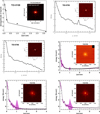 |
Fig. C.1 High-angular resolution imaging observations for TOI-5108 (upper left) and TOI-5786 (upper right, middle, and lower plots). For TOI- 5108 no secondary sources were detected. For TOI-5786 a secondary source at the separation ~1′′ was detected. |
Appendix D SED Plots
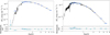 |
Fig. D.1 SED fits for TOI-5108 (left) and TOI-5786 (right). Blue points represent the flux values from available broadband photometry and the purple diamonds indicate the flux value of the synthetic photometry in the same passband. The best-fitting model is plotted in black. Residuals normalized to the errors of the photometry are shown below. |
References
- Ahrer, E., Queloz, D., Rajpaul, V. M., et al. 2021, MNRAS, 503, 1248 [NASA ADS] [CrossRef] [Google Scholar]
- Aigrain, S., & Foreman-Mackey, D. 2023, ARA&A, 61, 329 [NASA ADS] [CrossRef] [Google Scholar]
- Allard, F., Homeier, D., & Freytag, B. 2012, Philos. Trans. Roy. Soc. Lond. Ser. A, 370, 2765 [NASA ADS] [Google Scholar]
- Ambikasaran, S., Foreman-Mackey, D., Greengard, L., Hogg, D. W., & O’Neil, M. 2015, IEEE Trans. Pattern Anal. Mach. Intell., 38, 252 [Google Scholar]
- Attia, O., Bourrier, V., Eggenberger, P., et al. 2021, A&A, 647, A40 [EDP Sciences] [Google Scholar]
- Bailer-Jones, C. A. L., Rybizki, J., Fouesneau, M., Demleitner, M., & Andrae, R. 2021, AJ, 161, 147 [Google Scholar]
- Barragán, O., Aigrain, S., Kubyshkina, D., et al. 2019, MNRAS, 490, 698 [Google Scholar]
- Barragán, O., Gillen, E., Aigrain, S., et al. 2023, MNRAS, 522, 3458 [CrossRef] [Google Scholar]
- Batalha, N. E., Mandell, A., Pontoppidan, K., et al. 2017, PASP, 129, 064501 [Google Scholar]
- Beaugé, C., & Nesvorný, D. 2013, ApJ, 763, 12 [Google Scholar]
- Behr, P. R., France, K., Brown, A., et al. 2023, AJ, 166, 35 [NASA ADS] [CrossRef] [Google Scholar]
- Berger, T. A., Huber, D., van Saders, J. L., et al. 2020, AJ, 159, 280 [Google Scholar]
- Berger, T. A., Schlieder, J. E., & Huber, D. 2023, AJ, submitted [arXiv:2301.11338] [Google Scholar]
- Blunt, S., Carvalho, A., David, T. J., et al. 2023, AJ, 166, 62 [NASA ADS] [CrossRef] [Google Scholar]
- Boisse, I., Eggenberger, A., Santos, N. C., et al. 2010, A&A, 523, A88 [NASA ADS] [CrossRef] [EDP Sciences] [Google Scholar]
- Bouchy, F., Hébrard, G., Udry, S., et al. 2009, A&A, 505, 853 [NASA ADS] [CrossRef] [EDP Sciences] [Google Scholar]
- Bourque, M., Espinoza, N., Filippazzo, J., et al. 2021, The Exoplanet Characterization Toolkit (ExoCTK) [Google Scholar]
- Bourrier, V., Ehrenreich, D., King, G., et al. 2017, A&A, 597, A26 [NASA ADS] [CrossRef] [EDP Sciences] [Google Scholar]
- Bourrier, V., Lecavelier des Etangs, A., Ehrenreich, D., et al. 2018a, A&A, 620, A147 [NASA ADS] [CrossRef] [EDP Sciences] [Google Scholar]
- Bourrier, V., Lovis, C., Beust, H., et al. 2018b, Nature, 553, 477 [NASA ADS] [CrossRef] [Google Scholar]
- Bressan, A., Marigo, P., Girardi, L., et al. 2012, MNRAS, 427, 127 [NASA ADS] [CrossRef] [Google Scholar]
- Brown, T. M., Baliber, N., Bianco, F. B., et al. 2013, PASP, 125, 1031 [Google Scholar]
- Brucalassi, A., Grupp, F., Kellermann, H., et al. 2016, in SPIE Conf. Ser., 9908, 99085W [NASA ADS] [Google Scholar]
- Buchhave, L. A., Bakos, G. Á., Hartman, J. D., et al. 2010, ApJ, 720, 1118 [NASA ADS] [CrossRef] [Google Scholar]
- Buchhave, L. A., Latham, D., Johansen, A., et al. 2012, Nature, 486, 375 [NASA ADS] [CrossRef] [Google Scholar]
- Buchhave, L. A., Bizzarro, M., Latham, D. W., et al. 2014, Nature, 509, 593 [Google Scholar]
- Caldwell, D. A., Tenenbaum, P., Twicken, J. D., et al. 2020, RNAAS, 4, 201 [NASA ADS] [Google Scholar]
- Casagrande, L., & VandenBerg, D. A. 2014, MNRAS, 444, 392 [Google Scholar]
- Castelli, F., & Kurucz, R. L. 2003, in Modelling of Stellar Atmospheres, 210, eds. N. Piskunov, W. W. Weiss, & D. F. Gray, A20 [NASA ADS] [Google Scholar]
- Choi, J., Dotter, A., Conroy, C., et al. 2016, ApJ, 823, 102 [Google Scholar]
- Ciardi, D. R., Beichman, C. A., Horch, E. P., & Howell, S. B. 2015, ApJ, 805, 16 [NASA ADS] [CrossRef] [Google Scholar]
- Collins, K. 2019, in American Astronomical Society Meeting Abstracts, 233, 140.05 [NASA ADS] [Google Scholar]
- Collins, K. A., Kielkopf, J. F., Stassun, K. G., & Hessman, F. V. 2017, AJ, 153, 77 [Google Scholar]
- Correia, A. C. M., Bourrier, V., & Delisle, J. B. 2020, A&A, 635, A37 [NASA ADS] [CrossRef] [EDP Sciences] [Google Scholar]
- Courcol, B., Bouchy, F., Pepe, F., et al. 2015, A&A, 581, A38 [NASA ADS] [CrossRef] [EDP Sciences] [Google Scholar]
- Cutri, R. M., Skrutskie, M. F., van Dyk, S., et al. 2003, VizieR Online Data Catalog: 2MASS All-Sky Catalog of Point Sources (Cutri+ 2003), VizieR On-line Data Catalog: II/246 [Google Scholar]
- Dekany, R., Roberts, J., Burruss, R., et al. 2013, ApJ, 776, 130 [CrossRef] [Google Scholar]
- Dembinski, H., Ongmongkolkul, P., Deil, C., et al. 2023, https://doi.org/10.5281/zenodo.3949207 [Google Scholar]
- Dong, S., Xie, J.-W., Zhou, J.-L., Zheng, Z., & Luo, A. 2018, PNAS, 115, 266 [NASA ADS] [CrossRef] [Google Scholar]
- dos Santos, L. A., Ehrenreich, D., Bourrier, V., et al. 2019, A&A, 629, A47 [NASA ADS] [CrossRef] [EDP Sciences] [Google Scholar]
- Dos Santos, L. A., Vidotto, A. A., Vissapragada, S., et al. 2022, A&A, 659, A62 [NASA ADS] [CrossRef] [EDP Sciences] [Google Scholar]
- Dotter, A. 2016, ApJS, 222, 8 [Google Scholar]
- Eastman, J., Gaudi, B. S., & Agol, E. 2013, PASP, 125, 83 [Google Scholar]
- Ehrenreich, D., Bourrier, V., Wheatley, P. J., et al. 2015, Nature, 522, 459 [Google Scholar]
- Ehrhardt, J., Thomas, L., Kellermann, H., et al. 2024, A&A, 692, A220 [NASA ADS] [CrossRef] [EDP Sciences] [Google Scholar]
- Eisner, N. L., Barragán, O., Aigrain, S., et al. 2020, MNRAS, 494, 750 [NASA ADS] [CrossRef] [Google Scholar]
- Espinoza, N., Kossakowski, D., & Brahm, R. 2019, MNRAS, 490, 2262 [Google Scholar]
- Fahrenschon, V., Kellermann, H., Wang, L., et al. 2020, SPIE Conf. Ser., 11447, 114473H [NASA ADS] [Google Scholar]
- Foreman-Mackey, D., Agol, E., Ambikasaran, S., & Angus, R. 2017, AJ, 154, 220 [Google Scholar]
- Foster, G., Poppenhaeger, K., Ilic, N., & Schwope, A. 2022, A&A, 661, A23 [NASA ADS] [CrossRef] [EDP Sciences] [Google Scholar]
- France, K., Loyd, R. O. P., Youngblood, A., et al. 2016, ApJ, 820, 89 [NASA ADS] [CrossRef] [Google Scholar]
- Fulton, B. J., & Petigura, E. A. 2018, AJ, 156, 264 [Google Scholar]
- Fulton, B. J., Petigura, E. A., Blunt, S., & Sinukoff, E. 2018, PASP, 130, 044504 [Google Scholar]
- Furész, G., Szentgyorgyi, A., Latham, D., & Vinkó, J. 2008, PhD thesis, University of Szeged, Hungary [Google Scholar]
- Furlan, E., Ciardi, D. R., Everett, M. E., et al. 2017, AJ, 153, 71 [NASA ADS] [CrossRef] [Google Scholar]
- Gaia Collaboration 2020, VizieR Online Data Catalog: Gaia EDR3 (Gaia Collaboration, 2020), VizieR On-line Data Catalog: I/350 [Google Scholar]
- Giacalone, S., & Dressing, C. D. 2020, Astrophysics Source Code Library [record ascl:2002.004] [Google Scholar]
- Giacalone, S., Dressing, C. D., Jensen, E. L. N., et al. 2021, AJ, 161, 24 [Google Scholar]
- Green, G. M. 2018, J. Open Source Softw., 3, 695 [Google Scholar]
- Green, G. M., Schlafly, E., Zucker, C., Speagle, J. S., & Finkbeiner, D. 2019, ApJ, 887, 93 [NASA ADS] [CrossRef] [Google Scholar]
- Han, T., Robertson, P., Kanodia, S., et al. 2024, AJ, 167, 4 [CrossRef] [Google Scholar]
- Hauschildt, P. H., Allard, F., & Baron, E. 1999, ApJ, 512, 377 [Google Scholar]
- Hayward, T. L., Brandl, B., Pirger, B., et al. 2001, PASP, 113, 105 [NASA ADS] [CrossRef] [Google Scholar]
- Heidari, N., Boisse, I., Hara, N. C., et al. 2024, A&A, 681, A55 [NASA ADS] [CrossRef] [EDP Sciences] [Google Scholar]
- Helled, R. 2023, A&A, 675, L8 [NASA ADS] [CrossRef] [EDP Sciences] [Google Scholar]
- Howarth, I. D. 2011, MNRAS, 418, 1165 [NASA ADS] [CrossRef] [Google Scholar]
- Hsu, D. C., Ford, E. B., Ragozzine, D., & Ashby, K. 2019, AJ, 158, 109 [NASA ADS] [CrossRef] [Google Scholar]
- Huang, C. X., Vanderburg, A., Pál, A., et al. 2020a, RNAAS, 4, 204 [Google Scholar]
- Huang, C. X., Vanderburg, A., Pál, A., et al. 2020b, RNAAS, 4, 206 [NASA ADS] [Google Scholar]
- Huber, D., Zinn, J., Bojsen-Hansen, M., et al. 2017, ApJ, 844, 102 [Google Scholar]
- Husser, T. O., Wende-von Berg, S., Dreizler, S., et al. 2013, A&A, 553, A6 [NASA ADS] [CrossRef] [EDP Sciences] [Google Scholar]
- Ionov, D. E., Pavlyuchenkov, Y. N., & Shematovich, V. I. 2018, MNRAS, 476, 5639 [Google Scholar]
- Jackson, B., Arras, P., Penev, K., Peacock, S., & Marchant, P. 2017, ApJ, 835, 145 [NASA ADS] [CrossRef] [Google Scholar]
- Jenkins, J. M. 2002, ApJ, 575, 493 [Google Scholar]
- Jenkins, J. M., Chandrasekaran, H., McCauliff, S. D., et al. 2010, SPIE Conf. Ser., 7740, 77400D [Google Scholar]
- Jenkins, J. M., Twicken, J. D., McCauliff, S., et al. 2016, SPIE Conf. Ser., 9913, 99133E [Google Scholar]
- Jenkins, J. M., Tenenbaum, P., Seader, S., et al. 2020, Kepler Data Processing Handbook: Transiting Planet Search, Kepler Science Document KSCI-19081- 003 [Google Scholar]
- Jensen, E. 2013, Tapir: A web interface for transit/eclipse observability, Astrophysics Source Code Library [record ascl:1306.007] [Google Scholar]
- Kanodia, S., & Wright, J. 2018, RNAAS, 2, 4 [NASA ADS] [Google Scholar]
- Kellermann, H., Grupp, F., Brucalassi, A., et al. 2015, SPIE Conf. Ser., 9605, 96051R [NASA ADS] [Google Scholar]
- Kellermann, H., Grupp, F., Brucalassi, A., et al. 2016, SPIE Conf. Ser., 9908, 990863 [Google Scholar]
- Kellermann, H., Wang, L., Fahrenschon, V., et al. 2019, SPIE Conf. Ser., 11117, 111171O [Google Scholar]
- Kellermann, H., Wang, L., Fahrenschon, V., et al. 2020, SPIE Conf. Ser., 11447, 114474K [NASA ADS] [Google Scholar]
- Kempton, E.M. R., Bean, J. L., Louie, D. R., et al. 2018, PASP, 130, 114401 [CrossRef] [Google Scholar]
- Kipping, D. M. 2013, MNRAS, 435, 2152 [Google Scholar]
- Kite, E. S., Fegley, Bruce, J., Schaefer, L., & Ford, E. B. 2019, ApJ, 887, L33 [NASA ADS] [CrossRef] [Google Scholar]
- König, P. C., Damasso, M., Hébrard, G., et al. 2022, A&A, 666, A183 [NASA ADS] [CrossRef] [EDP Sciences] [Google Scholar]
- Korth, J., Gandolfi, D., Šubjak, J., et al. 2023, A&A, 675, A115 [NASA ADS] [CrossRef] [EDP Sciences] [Google Scholar]
- Koskinen, T. T., Lavvas, P., Huang, C., et al. 2022, ApJ, 929, 52 [NASA ADS] [CrossRef] [Google Scholar]
- Kreidberg, L. 2015, PASP, 127, 1161 [Google Scholar]
- Kunimoto, M., Huang, C., Tey, E., et al. 2021, RNAAS, 5, 234 [NASA ADS] [Google Scholar]
- Kunimoto, M., Tey, E., Fong, W., et al. 2022, RNAAS, 6, 236 [NASA ADS] [Google Scholar]
- Kurokawa, H., & Nakamoto, T. 2014, ApJ, 783, 54 [NASA ADS] [CrossRef] [Google Scholar]
- Kürster, M., Endl, M., Rouesnel, F., et al. 2003, A&A, 403, 1077 [NASA ADS] [CrossRef] [EDP Sciences] [Google Scholar]
- Kurucz, R. L. 1992, in The Stellar Populations of Galaxies, 149, eds. B. Barbuy, & A. Renzini, 225 [CrossRef] [Google Scholar]
- Kurucz, R. 1993, ATLAS9 Stellar Atmosphere Programs and 2 km/s grid. Kurucz CD-ROM No. 13 (Cambridge), 13 [Google Scholar]
- Lecavelier Des Etangs, A. 2007, A&A, 461, 1185 [NASA ADS] [CrossRef] [EDP Sciences] [Google Scholar]
- Lecavelier Des Etangs, A., Ehrenreich, D., Vidal-Madjar, A., et al. 2010, A&A, 514, A72 [NASA ADS] [CrossRef] [EDP Sciences] [Google Scholar]
- Lester, K. V., Howell, S. B., Ciardi, D. R., & Matson, R. A. 2022, AJ, 164, 56 [NASA ADS] [CrossRef] [Google Scholar]
- Li, J., Tenenbaum, P., Twicken, J. D., et al. 2019, PASP, 131, 024506 [NASA ADS] [CrossRef] [Google Scholar]
- Lightkurve Collaboration (Cardoso, J. V. d. M., et al.) 2018, Lightkurve: Kepler and TESS time series analysis in Python, Astrophysics Source Code Library [record ascl:1812.013] [Google Scholar]
- Lopez, E. D., & Fortney, J. J. 2014, ApJ, 792, 1 [Google Scholar]
- Lopez, E. D., Fortney, J. J., & Miller, N. 2012, ApJ, 761, 59 [Google Scholar]
- Loyd, R. O. P., France, K., Youngblood, A., et al. 2016, ApJ, 824, 102 [NASA ADS] [CrossRef] [Google Scholar]
- Lucy, L. B., & Sweeney, M. A. 1971, AJ, 76, 544 [NASA ADS] [CrossRef] [Google Scholar]
- Lundkvist, M. S., Kjeldsen, H., Albrecht, S., et al. 2016, Nat. Commun., 7, 11201 [Google Scholar]
- MacDougall, M. G., Petigura, E. A., Gilbert, G. J., et al. 2023, AJ, 166, 33 [NASA ADS] [CrossRef] [Google Scholar]
- Mansfield, M., Bean, J. L., Oklopcic, A., et al. 2018, ApJ, 868, L34 [NASA ADS] [CrossRef] [Google Scholar]
- Mantovan, G., Malavolta, L., Desidera, S., et al. 2024, A&A, 682, A129 [NASA ADS] [CrossRef] [EDP Sciences] [Google Scholar]
- Martin, D. C., Fanson, J., Schiminovich, D., et al. 2005, ApJ, 619, L1 [Google Scholar]
- Martioli, E., Hébrard, G., de Almeida, L., et al. 2023, A&A, 680, A84 [NASA ADS] [CrossRef] [EDP Sciences] [Google Scholar]
- Matsakos, T., & Königl, A. 2016, ApJ, 820, L8 [Google Scholar]
- Mazeh, T., Holczer, T., & Faigler, S. 2016, A&A, 589, A75 [NASA ADS] [CrossRef] [EDP Sciences] [Google Scholar]
- McCully, C., Volgenau, N. H., Harbeck, D.-R., et al. 2018, SPIE Conf. Ser., 10707, 107070K [Google Scholar]
- Millholland, S., Petigura, E., & Batygin, K. 2020, ApJ, 897, 7 [NASA ADS] [CrossRef] [Google Scholar]
- Mistry, P., Pathak, K., Lekkas, G., et al. 2023, MNRAS, 521, 1066 [NASA ADS] [CrossRef] [Google Scholar]
- Morley, C. V., Knutson, H., Line, M., et al. 2017, AJ, 153, 86 [NASA ADS] [CrossRef] [Google Scholar]
- Morton, T. D. 2015, isochrones: Stellar model grid package, Astrophysics Source Code Library [record ascl:1503.010] [Google Scholar]
- Moutou, C., Almenara, J. M., Hébrard, G., et al. 2021, A&A, 653, A147 [NASA ADS] [CrossRef] [EDP Sciences] [Google Scholar]
- Murray, C. D., & Dermott, S. F. 1999, Solar System Dynamics [Google Scholar]
- Narita, N., Fukui, A., Kusakabe, N., et al. 2019, J. Astron. Telesc. Instrum. Syst., 5, 015001 [NASA ADS] [Google Scholar]
- Nicholson, B. A., & Aigrain, S. 2022, MNRAS, 515, 5251 [NASA ADS] [CrossRef] [Google Scholar]
- Ninan, J. P., Stefansson, G., Mahadevan, S., et al. 2020, ApJ, 894, 97 [Google Scholar]
- Nowak, G., Palle, E., Gandolfi, D., et al. 2020, MNRAS, 497, 4423 [NASA ADS] [CrossRef] [Google Scholar]
- Oklopčić, A. 2019, ApJ, 881, 133 [Google Scholar]
- Oklopčić, A., & Hirata, C. M. 2018, ApJ, 855, L11 [Google Scholar]
- Owen, J. E. 2019, Annu. Rev. Earth Planet. Sci., 47, 67 [CrossRef] [Google Scholar]
- Owen, J. E., & Jackson, A. P. 2012, MNRAS, 425, 2931 [Google Scholar]
- Owen, J. E., & Lai, D. 2018, MNRAS, 479, 5012 [Google Scholar]
- Owen, J. E., & Murray-Clay, R. 2018, MNRAS, 480, 2206 [NASA ADS] [CrossRef] [Google Scholar]
- Owen, J. E., & Wu, Y. 2013, ApJ, 775, 105 [Google Scholar]
- Paegert, M., Stassun, K. G., Collins, K. A., et al. 2022, VizieR Online Data Catalog: TESS Input Catalog version 8.2 (TIC v8.2) (Paegert+, 2021), VizieR On-line Data Catalog: IV/39 [Google Scholar]
- Palle, E., Nortmann, L., Casasayas-Barris, N., et al. 2020, A&A, 638, A61 [EDP Sciences] [Google Scholar]
- Parker, E. N. 1958, ApJ, 128, 664 [Google Scholar]
- Parviainen, H. 2015, MNRAS, 450, 3233 [Google Scholar]
- Parviainen, H. 2020, MNRAS, 499, 1633 [NASA ADS] [CrossRef] [Google Scholar]
- Parviainen, H., & Korth, J. 2020, MNRAS, 499, 3356 [NASA ADS] [CrossRef] [Google Scholar]
- Parviainen, H., Tingley, B., Deeg, H. J., et al. 2019, A&A, 630, A89 [NASA ADS] [CrossRef] [EDP Sciences] [Google Scholar]
- Patel, J. A., & Espinoza, N. 2022, AJ, 163, 228 [NASA ADS] [CrossRef] [Google Scholar]
- Perruchot, S., Kohler, D., Bouchy, F., et al. 2008, SPIE Conf. Ser., 7014, 70140J [Google Scholar]
- Petigura, E. A., Howard, A. W., Lopez, E. D., et al. 2016, ApJ, 818, 36 [Google Scholar]
- Petigura, E. A., Sinukoff, E., Lopez, E. D., et al. 2017, AJ, 153, 142 [NASA ADS] [CrossRef] [Google Scholar]
- Petigura, E. A., Benneke, B., Batygin, K., et al. 2018a, AJ, 156, 89 [Google Scholar]
- Petigura, E. A., Marcy, G. W., Winn, J. N., et al. 2018b, AJ, 155, 89 [Google Scholar]
- Petigura, E. A., Livingston, J., Batygin, K., et al. 2020, AJ, 159, 2 [NASA ADS] [CrossRef] [Google Scholar]
- Pfeiffer, M. J., Frank, C., Baumueller, D., Fuhrmann, K., & Gehren, T. 1998, A&AS, 130, 381 [NASA ADS] [CrossRef] [EDP Sciences] [Google Scholar]
- Pizzolato, N., Maggio, A., Micela, G., Sciortino, S., & Ventura, P. 2003, A&A, 397, 147 [NASA ADS] [CrossRef] [EDP Sciences] [Google Scholar]
- Pope, B. J. S., Parviainen, H., & Aigrain, S. 2016, MNRAS, 461, 3399 [Google Scholar]
- Poppenhaeger, K., Ketzer, L., & Mallonn, M. 2021, MNRAS, 500, 4560 [Google Scholar]
- Puranam, A., & Batygin, K. 2018, AJ, 155, 157 [CrossRef] [Google Scholar]
- Quinn, S. N., White, R. J., Latham, D. W., et al. 2012, ApJ, 756, L33 [NASA ADS] [CrossRef] [Google Scholar]
- Rajpaul, V. M., Buchhave, L. A., Lacedelli, G., et al. 2021, MNRAS, 507, 1847 [NASA ADS] [CrossRef] [Google Scholar]
- Rein, H., & Liu, S. F. 2012, A&A, 537, A128 [NASA ADS] [CrossRef] [EDP Sciences] [Google Scholar]
- Rein, H., & Spiegel, D. S. 2015, MNRAS, 446, 1424 [Google Scholar]
- Ribas, I., Tuomi, M., Reiners, A., et al. 2018, Nature, 563, 365 [Google Scholar]
- Ricker, G. R., Winn, J. N., Vanderspek, R., et al. 2015, J. Astron. Telesc. Instrum. Syst., 1, 014003 [Google Scholar]
- Sanchis-Ojeda, R., Rappaport, S., Winn, J. N., et al. 2014, ApJ, 787, 47 [Google Scholar]
- Santos, N. C., Sousa, S. G., Mortier, A., et al. 2013, A&A, 556, A150 [NASA ADS] [CrossRef] [EDP Sciences] [Google Scholar]
- Schlafly, E. F., & Finkbeiner, D. P. 2011, ApJ, 737, 103 [Google Scholar]
- Schlegel, D. J., Finkbeiner, D. P., & Davis, M. 1998, ApJ, 500, 525 [Google Scholar]
- Serrano Bell, J., Díaz, R. F., Hébrard, G., et al. 2024, A&A, 684, A6 [NASA ADS] [CrossRef] [EDP Sciences] [Google Scholar]
- Smith, J. C., Stumpe, M. C., Van Cleve, J. E., et al. 2012, PASP, 124, 1000 [Google Scholar]
- Sousa, S. G., Adibekyan, V., Delgado-Mena, E., et al. 2021, A&A, 656, A53 [NASA ADS] [CrossRef] [EDP Sciences] [Google Scholar]
- Spake, J. J., Sing, D. K., Evans, T. M., et al. 2018, Nature, 557, 68 [Google Scholar]
- Speagle, J. S. 2020, MNRAS, 493, 3132 [Google Scholar]
- Stefànsson, G., Mahadevan, S., Petrovich, C., et al. 2022, ApJ, 931, L15 [NASA ADS] [CrossRef] [Google Scholar]
- Strakhov, I. A., Safonov, B. S., & Cheryasov, D. V. 2023, Astrophys. Bull., 78, 234 [NASA ADS] [CrossRef] [Google Scholar]
- Stumpe, M. C., Smith, J. C., Van Cleve, J. E., et al. 2012, PASP, 124, 985 [Google Scholar]
- Stumpe, M. C., Smith, J. C., Catanzarite, J. H., et al. 2014, PASP, 126, 100 [Google Scholar]
- Szabó, G. M., & Kiss, L. L. 2011, ApJ, 727, L44 [Google Scholar]
- Tal-Or, L., Trifonov, T., Zucker, S., Mazeh, T., & Zechmeister, M. 2019, MNRAS, 484, L8 [Google Scholar]
- Tamayo, D., Rein, H., Shi, P., & Hernandez, D. M. 2020, MNRAS, 491, 2885 [NASA ADS] [CrossRef] [Google Scholar]
- Tokovinin, A. 2018, PASP, 130, 035002 [Google Scholar]
- Trifonov, T., Kürster, M., Zechmeister, M., et al. 2018, A&A, 609, A117 [NASA ADS] [CrossRef] [EDP Sciences] [Google Scholar]
- Trifonov, T., Tal-Or, L., Zechmeister, M., et al. 2020, A&A, 636, A74 [NASA ADS] [CrossRef] [EDP Sciences] [Google Scholar]
- Trotta, R. 2008, Contemp. Phys., 49, 71 [Google Scholar]
- Vidal-Madjar, A., Lecavelier des Etangs, A., Désert, J. M., et al. 2003, Nature, 422, 143 [Google Scholar]
- Vines, J. I., & Jenkins, J. S. 2022, MNRAS, 513, 2719 [NASA ADS] [CrossRef] [Google Scholar]
- Vissapragada, S., Knutson, H. A., Greklek-McKeon, M., et al. 2022, AJ, 164, 234 [NASA ADS] [CrossRef] [Google Scholar]
- Wang, L., Grupp, F., Kellermann, H., et al. 2016, SPIE Conf. Ser., 9913, 99133O [NASA ADS] [Google Scholar]
- Wang, L., Grupp, F., Kellermann, H., Hopp, U., & Bender, R. 2017, SPIE Conf. Ser., 10400, 104001V [Google Scholar]
- Watson, A. J., Donahue, T. M., & Walker, J. C. 1981, Icarus, 48, 150 [Google Scholar]
- Wizinowich, P., Acton, D. S., Shelton, C., et al. 2000, PASP, 112, 315 [NASA ADS] [CrossRef] [Google Scholar]
- Wright, E. L., Eisenhardt, P. R. M., Mainzer, A. K., et al. 2010, AJ, 140, 1868 [Google Scholar]
- Yee, S. W., Petigura, E. A., & von Braun, K. 2017, ApJ, 836, 77 [Google Scholar]
- Youngblood, A., France, K., Loyd, R. O. P., et al. 2016, ApJ, 824, 101 [Google Scholar]
- Zechmeister, M., & Kürster, M. 2009, A&A, 496, 577 [CrossRef] [EDP Sciences] [Google Scholar]
- Zechmeister, M., Reiners, A., Amado, P. J., et al. 2018, A&A, 609, A12 [NASA ADS] [CrossRef] [EDP Sciences] [Google Scholar]
- Zhang, K., & Hamilton, D. P. 2008, Icarus, 193, 267 [Google Scholar]
- Ziegler, C., Tokovinin, A., Briceño, C., et al. 2020, AJ, 159, 19 [Google Scholar]
TOI-5786 b is outside the parameter space of the Millholland et al. (2020) model (1-70 M⊕) and is therefore not included in this analysis.
All Tables
Bayesian evidence values for the different GP models fitted to the TESS data of TOI-5786.
X-ray and EUV fluxes and the corresponding mass-loss rates derived from the three proxy spectra for both planets.
Comparison of the derived stellar parameters in Section 3.2 using SED and isochrone fitting.
All Figures
|
Fig. 1 PDCSAP from the TESS light curves for TOI-5108 (upper plot) and TOI-5786 (lower plot). For the last sectors for both targets where high cadence photometry is available, we show the 120 second cadence in grey and the flux data binned to the 10-minute cadence in black. |
| In the text | |
|
Fig. 2 SAP flux of TOI-5108 and TOI-5786. The lower plot shows the light curve of TOI-5786, which has strong systematics at the edges and an offset between the two sectors. For TOI-5108, the systematics are less severe (upper plot). |
| In the text | |
|
Fig. 3 GLS periodograms of TOI-5108 and TOI-5786. The top periodograms belong to TOI-5108. The first and second rows are the RV data from MaHPS and SOPHIE before and after subtracting the signal of the transiting planet. The next three rows show the periodograms of the activity indicators derived from the SOPHIE spectra (BIS) and MaHPS spectra (Ca IRT). The last row shows the periodogram of the TESS data. The dotted red line shows the period of the transiting planet and the dotted black line is located at the 0.1% FAP. Bottom periodograms are the same as the top ones but for TOI-5786. |
| In the text | |
|
Fig. 4 Spectral type classification of TOI-5786 and the detected companion. Using the AO imaging, the 2MASS magnitudes have been deblended and the two stars have been placed on a JHKs color–color diagram. |
| In the text | |
|
Fig. 5 Result of the juliet fit of TOI-5108. Upper panel: radial velocity curve of TOI-5108 with the best fit Keplerian model for TOI-5108 b in black. Middle panel: phase-folded radial velocity curve. The dark blue data points represent the MaHPS RV data binned at 0.05 phases. Light blue is the unbinned MaHPS data and red is the SOPHIE data. Lower Panel: Residuals after subtracting the signal of TOI-5108 b. |
| In the text | |
|
Fig. 6 TESS light curve of TOI-5786 before and after the GP correction. Top row: TESS light curve of TOI-5786 with the GP + transit model. Middle row: TESS light curve with the GP model subtracted showing only the transits of the two planet candidates. Bottom row: phase-folded lightcurves of the TESS Object of Interest TOI-5786.01 on the right and our detected planet candidate on the left. |
| In the text | |
|
Fig. 7 Results of the juliet fit of TOI-5786. First panel: radial velocity curve of TOI-5786 with the best fit Keplerian model for the two-planet case in black. Second panel: RVs phase-folded to TOI-5786 b. The dark blue data points represent the MaHPS RV data binned at 0.05 phases. Third Panel: RVs phase-folded to the period of the inner companion candidate. Fourth Panel: Residuals after subtracting the signals of both planets. |
| In the text | |
|
Fig. 8 Population of known transiting exoplanets with masses and radii measured to 33% or better taken from the NASA Exoplanet Archive (accessed on 14.10.2024). TOI-5108 b and TOI-5786 b are shown with black stars. The position of the planet candidate around TOI-5786 is shown with a white star. The dotted brown line indicates the boundaries of the Neptune desert as defined by Mazeh et al. (2016). |
| In the text | |
|
Fig. 9 Estimate of the envelope mass fraction, fenv, of TOI-5108 b using the model from Millholland et al. (2020). The grey bar is the calculated envelope fraction with the associated error in the tides-free model. The shaded regions show the 2-σ contours of the envelope fraction for different obliquities, λ. |
| In the text | |
|
Fig. 10 Simulated transit observation with NIRSpec for the helium triplet absorption signals calculated with p-winds. The helium absorption models shown are for the high XUV input spectrum (WASP-17) with the largest mass-loss rates. |
| In the text | |
|
Fig. A.1 Transit light curves of TOI-5108 (left) and TOI-5786 (right). The TESS light curves are phase-folded with the data from all available sectors. |
| In the text | |
|
Fig. C.1 High-angular resolution imaging observations for TOI-5108 (upper left) and TOI-5786 (upper right, middle, and lower plots). For TOI- 5108 no secondary sources were detected. For TOI-5786 a secondary source at the separation ~1′′ was detected. |
| In the text | |
|
Fig. D.1 SED fits for TOI-5108 (left) and TOI-5786 (right). Blue points represent the flux values from available broadband photometry and the purple diamonds indicate the flux value of the synthetic photometry in the same passband. The best-fitting model is plotted in black. Residuals normalized to the errors of the photometry are shown below. |
| In the text | |
Current usage metrics show cumulative count of Article Views (full-text article views including HTML views, PDF and ePub downloads, according to the available data) and Abstracts Views on Vision4Press platform.
Data correspond to usage on the plateform after 2015. The current usage metrics is available 48-96 hours after online publication and is updated daily on week days.
Initial download of the metrics may take a while.